1
Chapter
Preparing for Acquisition
2
Goto
Sample Preparation
2.1
The quality of the sample can have a significant impact on the quality of its NMR
spectrum. The following is a brief list of suggestions to ensure high sample quality.
Always use clean and dry sample tubes to avoid contaminating the sample.
Always use good to high quality sample tubes to avoid unnecessary
difficulties in shimming.
Filter the sample solution.
Always use the same sample volume or solution height. This minimizes the
shimming that needs to be done between sample changes. Recommended
values are for 5 mm tubes: 0.6 ml or 4 cm of solution, and for 10 mm tubes:
4.0 ml or 4 cm of solution.
Use the depth gauge to position the sample tube correctly in the spinner.
This is discussed further in Chapter 5 ‘Sample Positioning’ of the BSMS
User’s Manual.
Check that the sample tube is held tightly in the spinner so that it does not
slip during an experiment.
Wipe the sample tube clean before inserting it into the magnet.
For experiments using sample spinning, be sure the spinner, especially the
reflectors, is clean. This is important so that the correct spinning rate can be
maintained.
Tuning and Matching the Probehead
2.2
Once the sample is inserted, the probehead should be tuned and matched. Notice
that correct tuning and matching is especially important for higher frequencies. In
general, the probehead should be tuned and matched each time a new sample is
inserted, each time a new probehead is put in the magnet, and each time the observe
or decouple nucleus is changed when using a broadband probe.
In a probehead there is a resonant circuit for each observe and decouple nucleus
indicated on the probehead label (e.g., one for 1H and one for 13C in a dual 1 H/13 C
probehead; one for 1 H and one for a wide range of nuclei in a BBO probehead).
There is also a resonant circuit for the lock nucleus, but the standard user will never
need to adjust this, so we will ignore it for now. Each of these circuits has a
frequency at which it is most sensitive (the resonance frequency). Tuning is the
process of adjusting this frequency until it coincides with the frequency of the
pulses transmitted to the circuit. For example, the frequency at which the 1 H
resonant circuit is most sensitive must be set to the carrier frequency of the 1 H
pulses (which is sfo1 if the 1 H circuit is connected to the f1 channel, sfo2 if it is
connected to the f2 channel, etc.). A probehead is said to be tuned when all of its
resonant circuits are tuned. Once a probehead has been tuned, it is not necessary to
retune it after slight adjustments to the carrier frequency, since the probehead is
AVANCE User’s Guide
Bruker
11
Goto
Preparing for Acquisition
generally tuned over a range of a couple MHz. On the other hand, large adjustments
to the carrier frequency, necessary when changing nuclei, do warrant retuning the
probehead, so a broadband probe needs to be retuned each time the heteronucleus is
changed.
Matching is the process of adjusting the impedance of the resonant circuit until it
corresponds with the impedance of the transmission line connected to it. This
impedance is 50 Ω . Correct matching minimizes the power that is reflected by the
probehead, and so is lost; or equivalently, maximizes the power that is transmitted
to the coil, and so is available to do NMR. A probehead is said to be matched when
all of its resonant circuits are matched. Again, once a probehead has been matched,
it is not necessary to rematch it after slight adjustments to the carrier frequency. On
the other hand, large adjustments to the carrier frequency, necessary when changing
nuclei, do warrant rematching the probehead.
Tuning and matching are carried out simultaneously using the XWIN-NMR
command wobb (wobble). During wobbling, a low power signal is transmitted to
the probehead. This signal is swept over a frequency range determined by the
parameter wbsw (the default value is 4 MHz) centered on the carrier frequency (i.e.,
sfo1, sfo2, etc., depending on which nucleus is being tuned/matched). Within the
preamp (High Performance Preamplifier Assembly or HPPR), the impedance of the
probe over this frequency range is compared to the impedance of a 50Ω resistor.
The results are shown both on the LED display of the HPPR and in the acquisition
submenu in XWIN-NMR. Both displays show the reflected power of the probehead
versus the frequency of the signal. The user observes either one or both of these
displays while tuning and matching the probehead.
Tuning and Matching 1 H
2.2.1
When the NMR experiments to be performed are 1 H homonuclear experiments (e.g.,
1 H 1D spectroscopy, COSY, NOESY, or TOCSY), it is only necessary to tune and
match the 1H circuit of the probehead.
Make sure that the sample is in the magnet, and the probehead is connected for
standard 1 H acquisition. Note that there is no special configuration for tuning and
matching. Also, it is recommended to tune and match without sample spinning.
Set the parameters
In XWIN-NMR, enter edsp and set the following spectrometer parameters:
NUC1
NUC2
NUC3
1H
OFF
OFF .
This automatically sets sfo1 to a frequency appropriate for 1H tuning and
matching. There is no need to adjust sfo1 carefully now. Exit edsp by clicking
SAVE.
Other wobb parameters are wbsw, which determines the wobble sweep width in
MHz (the default value is 4 MHz), and wbst, which determines the number of
wobble steps over the sweep width (the default value is 256). Both of these
parameters may be found in the eda table. No other parameters are required.
Start wobbling
12
Bruker
AVANCE User’s Guide
Goto
Tuning and Matching the Probehead
Before starting the wobbling procedure, ensure that no acquisition is in progress,
e.g., enter stop.
Enter acqu to switch to the acquisition window of XWIN-NMR, if it is desired to
use this to monitor the tuning and matching. Notice that being in the acquisition
window slows down the wobbling procedure, so if the HPPR LED display will be
used to monitor tuning and matching, it is best to remain in the main XWIN-NMR
window and not switch to the acquisition window.
Start the frequency sweep by typing wobb. The curve that appears in the acquisition
window is the reflected power as a function of frequency. Unless the probehead is
quite far from the correct tuning and matching, there will be a noticeable dip in the
curve. When the 1H circuit is properly tuned, the dip will be in the center of the
window, denoted by the vertical marker; and when the circuit is properly matched,
the dip will extend all the way down to the x axis. Similar information is conveyed
by the LED display on the HPPR. The horizontal row of LED’s indicates tuning and
the vertical row matching. When the circuit is properly tuned and matched, the
number of LED’s lit is minimized. This usually means that only green LED’s, not
red, are lit in both the horizontal and vertical displays.
Tune and match
Adjust the tuning and matching screws (labeled T and M) at the base of the
probehead with the special tool provided. Note that the screws are color coded and
those for the 1 H circuit are usually yellow. Also note that the screws have a limited
range and attempting to turn them beyond this range will damage the probehead.
Since there is interplay between tuning and matching, it is generally useful to adjust
the T and M screws in an iterative fashion. Turn the M screw until the dip is well
matched at some frequency (the dip extends to the x axis and the number of LED’s
lit in the vertical HPPR display is minimized). Most likely this will not be the
desired frequency. Adjust the T screw slightly to move the dip toward the center of
the window, or equivalently, to reduce the number of LED’s lit in the horizontal
HPPR display. Rematch the dip by adjusting the M screw. Again, adjust T to move
the dip towards the center of the screen and rematch using M. In this manner,
continue walking the dip towards the correct resonance frequency. Note that it is
possible to run out of range on the M screw. If this happens, return M to the middle
of its range, adjust T to get a well matched dip at some frequency, and walk the dip
towards the correct frequency as described above.
As mentioned above, ideal tuning and matching is when the dip is centered in the
window and extends to y = 0 (the x axis) on the acquisition window, or equivalently,
when the number of LED’s lit on the preamp is minimized in both the vertical and
horizontal display.
When the 1H circuit is tuned and matched, exit the wobble routine by typing stop.
Click on return to exit the acquisition window and return to the main window.
Tuning and Matching
13
C
2.2.2
Since most 13C experiments make use of 1 H decoupling, when tuning and matching
a probehead for 13 C, it is generally a good idea also to tune and match for 1H.
When tuning and matching a probehead with multiple resonant circuits, it is best
first to tune and match the lowest frequency circuit and then to proceed to higher
AVANCE User’s Guide
Bruker
13
Goto
Preparing for Acquisition
frequency circuits. The larger capacitors and inductors found in lower frequency
resonant circuits can be expected to have larger stray capacitance and inductance
than the smaller elements in higher frequency circuits. Thus, one would expect
tuning and matching lower frequency circuits to affect the tuning and matching of
higher frequency circuits more so than vice versa. So when tuning and matching a
probehead for both 1H and 13 C, it is best to make the 13C adjustments first and the
1 H adjustments last.
Make sure that the sample is in the magnet, and the probehead is connected for the
appropriate experiment. Also, it is recommended to tune and match without sample
spinning.
Set the parameters
In XWIN-NMR, enter edsp and set the following spectrometer parameters:
NUC1
NUC2
NUC3
13C
OFF
OFF .
This automatically sets sfo1 to a frequency appropriate for
matching. Exit edsp by clicking SAVE.
13 C
tuning and
Other wobb parameters are wbsw and wbst, as mentioned above. Both of these
parameters may be found in the eda table. No other parameters are required.
Start wobbling, tune and match
Ensure that no acquisition is in progress, e.g., enter stop.
Enter acqu to switch to the acquisition window, if this will be used to monitor the
tuning and matching.
Start the frequency sweep by typing wobb. The curve that appears in the acquisition
window is for 13C. Adjust the tuning and matching following the guidelines given
above for 1H. Notice that some probeheads (e.g., broadband probeheads) have
sliding bars instead of screws, one set labeled tuning and another matching. These
probeheads also have a menu of tuning and matching values for several nuclei. Set
the tuning and matching sliding bars to the values indicated for 13 C on the menu.
Adjust the tuning bar until the dip is well matched at some frequency, and then walk
the dip towards the correct frequency as described above for 1H.
Once the 13C circuit is tuned and matched, the 13C wobbling must be stopped and
1 H wobbling begun. One straightforward way to do this is as follows: Exit the
wobble routine by typing stop. Enter edsp, change to NUC1 to 1H, and exit by
clicking SAVE. Then start the 1 H frequency sweep by typing wobb. After a few
seconds the 1H curve appears in the acquisition window and the 1 H circuit can be
tuned and matched as described above.
Alternatively, if the user already has a data set in which NUC1 = 1H and NUC2 =
OFF, there is no need to redo edsp for the current data set. The user may simply
read in the 1 H data set and then type wobb.
Once the probehead is tuned and matched for 13 C and 1H, exit the wobble routine by
typing stop.
Click on return to exit the acquisition window and return to the main window.
14
Bruker
AVANCE User’s Guide
Goto
Locking and Shimming
Locking and Shimming
2.3
Before running an NMR experiment, it is also necessary to lock and shim the
magnetic field.
Locking
To display the lock signal enter lockdisp . This opens a new window in which the
lock trace now appears.
The most convenient way for the standard user to lock is semi-automatically using
the XWIN-NMR command lock. To start the lock-in procedure, enter lock and
select the appropriate solvent from the menu that appears. Alternatively, enter the
solvent name with the lock command, e.g., lock cdcl3. During lock-in, the lock
power, field value, and frequency shift for the solvent are set according to the
values in the 2H-Lock table (also known as the edlock table). These values can be
edited with the command edlock. Note that the lock power listed in this table is
the level used once lock-in has been achieved. The field-shift mode is then selected
and autolock is activated. Once lock-in is achieved, the lock gain is set so that the
lock signal is visible in the lock window. At this point the message “lock: finished”
appears in the status line at the bottom of the window.
The lock-in procedure outlined above sets the frequency shift to the exact frequency
shift value for the given solvent as listed in the edlock table. It also sets the field
value to the value (which is the same for all solvents) listed in the edlock table
and then adjusts this slightly to achieve lock-in. As a result, the absolute magnetic
field is now nearly the same no matter what lock solvent is used. This has the
advantage that offsets can now be defined in ppm, since the absolute frequency
corresponding to a given ppm value no longer depends on the lock solvent.
Another advantage of following this lock-in procedure is that it automatically sets
the parameter solvent correctly in the eda table. This is especially important if
you wish to use the automatic calibration command sref, as described later (see
“Spectrum Calibration and Optimization” on page 25).
It is recommended that each time the probehead is changed, the user adjust the
phase of the lock signal while monitoring the sweep wiggles (i.e., while the field is
not locked but is being swept). This is necessary if the original lock phase is very
far wrong, in which case autolock may fail to achieve lock-in. If the original phase
is reasonably close to correct, then lock-in can be achieved and the phase can be
adjusted afterwards using autophase. Please note that the lock phase for each
probehead is stored in the edlock table. To make shure that XWIN-NMR selects
the edlock table assigned to the current probe, enter edhead,then click on
Define Current and select your current probe.
The other lock parameter that may possibly be problematic when using the XWINNMR lock command is the lock power. In some instances, the power level listed in
the edlock table is too high, meaning that the lock signal is always saturated.
Usually, in this situation lock-in can be achieved, but since the signal is saturated, it
oscillates. A quick fix is simply to reduce the lock power by hand once lock-in has
been achieved. A better fix is to change the power level in the edlock table. Note
that the appropriate lock power level depends on the lock solvent, the field value,
and the probehead.
Shimming
AVANCE User’s Guide
Bruker
15
Goto
Preparing for Acquisition
If the probehead has just been changed, the first step in shimming the magnetic field
is to read in the shim file corresponding to the new probehead. Enter rsh and then
select the appropriate file from the menu that appears.
Assuming that the shim file is a good one, or that a prior user has shimmed the field
for the current probehead, the user need only adjust the Z and Z 2 shims (and
possibly the X and Y). Generally, the shims are adjusted while viewing the lock
signal and the best shim values correspond to the highest lock level (height of the
lock signal in the window). For further discussion of shimming see Chapter 6 ‘Shim
Operation’ of the BSMS User’s Manual.
Optimize lock settings (optional)
Once the magnetic field has been locked and shimmed, the user may wish to
optimize the lock settings as described below. It is strongly recommended to follow
this procedure before running any experiment requiring optimal stability (e.g., NOE
difference experiments).
After the field is locked and shimmed, start the auto-power routine from the BSMS
keyboard (see Chapter 2 ‘Key Description’ of the BSMS User’s Manual). For lock
solvents with long T 1 relaxation times (e.g., CDCl3), however, auto power may take
an unacceptably long time and the lock power should be optimized manually.
Simply increase the lock power level until the signal begins to oscillate (i.e., until
saturation), and then reduce the power level slightly (approximately 3 dB). For
example, if the lock signal begins to oscillate at a power of –15 dB, the optimal
magnetic field stability can be expected when a level of approximately –18 dB (or
even –20 dB) is used. The field stability will be significantly worse if a power level
of, say, –35dB is used instead.
When the lock power is optimized, start the auto-phase routine, and finally the autogain routine. Take note of the gain value determined by auto gain. Using this value,
select the appropriate values for the loop filter, loop gain, and loop time as shown
below in Table 2.
16
Bruker
AVANCE User’s Guide
Goto
Locking and Shimming
Table 2. Lock Parameters (BSMS Firmware Version 940614)
Lock RX Gain
(after auto gain)
[dB]
Loop Filter
[Hz]
Loop Gain
[dB]
Loop Time
[sec]
120
20
–17.9
0.681
30
–14.3
0.589
50
–9.4
0.464
70
–6.6
0.384
100
–3.7
0.306
160
0.3
0.220
250
3.9
0.158
400
7.1
0.111
600
9.9
0.083
1000
13.2
0.059
1500
15.2
0.047
2000
16.8
0.041
110
90
So, for example if auto gain determines a lock gain of 100dB, the user should set
the loop filter to 160 Hz, the loop gain to 0.3 dB, and the loop time to 0.220 sec (see
Chapter 4 ‘Menu Description’ of the BSMS User’s Manual for how to set these
parameters from the BSMS keyboard).
AVANCE User’s Guide
Bruker
17
Goto
Preparing for Acquisition
18
Bruker
AVANCE User’s Guide