Download Chase Blokker, Software Engineer Nicole Klee, Experiment

on different days (therefore different weather), the calculated altitudes of which remained quite
similar.
For the temperature measurements a large factor was time and weather. The launch was
conducted midmorning and took over an hour for the full ascent and descent. Simply by looking
at the temperature readings on the ascent compared to the temperature readings on the descent it
is clear that the outside temperature had warmed significantly over the course of the morning.
Another factor in explaining the fluctuations of the temperature probe may have been whether
the probe was in direct sunlight or was facing away from the Sun and in the shadow of the
gondola. One way the authors could have better conducted this measurement would have been to
add a light sensor next to the temperature probe so they could track when the temperature probe
was facing towards or away from the Sun.
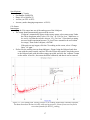
The carbon dioxide readings seemed to be fairly consistent. The main inaccuracy with
these was the carbon dioxide sensor’s high exposure to humans immediately prior to launch. As
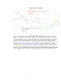
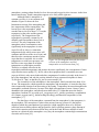
demonstrated by Figure 10, the carbon dioxide readings were very high at the beginning of the
ascent, but decreased rapidly over the first ten or twenty meters. It is believed that, because there
were so many people near the sensor during launch, all of whom were breathing out carbon
dioxide, the carbon dioxide readings were initially much higher than they should have been. The
carbon dioxide sensor takes time to adjust and for new air to flow through it, replacing the
carbon dioxide-filled air with normal air, so the readings for the first twenty or thirty meters of
altitude are probably much higher than they should have been.
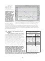
Despite these inaccuracies, the data generally matched the expected results. Both curve
fits for the pressure vs. altitude graph (Figure 8) approximated atmospheric pressure at ground
level to be 100 kPa. Given that atmospheric pressure is 101.325 kPa, that pressure can vary
significantly with weather, and that the altitude measurements were only accurate to two
significant figures, the pressure vs. altitude results were as accurate as possible. The pressure vs.
altitude data was extremely consistent; the error on the curve fits was less than 0.1%, and every
single error bar intersected both curves. These results also demonstrate that both the exponential
model and NASA’s empirical formula accurately model pressures at varying altitudes, while the
fact that the two curves were essentially identical
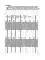
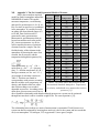
Molar Mass of Most Common
demonstrates how closely empirical data matches theory
Gases in the Atmosphere
for pressures in the atmosphere.
Molar
Gas
The temperature data was the least consistent of
Mass
the three sets; not only did the readings vary significantly
Carbon Dioxide CO2
44.01
between the ascent and descent, but they fluctuated
Argon
Ar
39.95
wildly throughout both the ascent and descent. Therefore,
Oxygen
O2
32.00
the NASA empirical model for temperatures does not
seem to accurately reflect the data, as demonstrated by
Nitrogen
N2
28.01
the fact that, in Figure 9, very few of the error bars
Neon
Ne
20.18
intersect their respective best-fit curves. However, it is
Water Vapor
H2 O
18.02
possible that, if the error bars were to take into account
the unquantifiable errors discussed above, they would in
Methane
CH4
16.04
fact intersect the best fit curves; it is still possible that the
Helium
He
4.00
NASA empirical model is the best curve fit for this data.
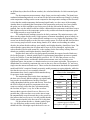
Table 2: This chart lists the most
For the carbon dioxide vs. altitude graph (Figure
common gases in Earth's
10), it is difficult to predict exactly what the results
atmosphere and their molar masses
should look like. One might expect the best fit curve to
[7].
13