1
LRmix Studio user manual
December 15th, 2014
1. What is LRmix Studio?
LRmix Studio is a free of charge, open-source (GPLv 3 license), expert system dedicated to
the interpretation of forensic DNA profiles, with a particular focus on complex DNA
mixtures. LRmix Studio enables measuring the probative value of any (autosomal STR-based)
forensic DNA sample.
LRmix Studio is programmed after the likelihood ratio model described in Haned et al (FSIG
2012) and Gill & Haned (FSIG 2013). This model explicitly accommodates for uncertainty in
the DNA profiles from the allelic drop-out and drop-in phenomena. The program estimates
these quantities from the available data, and uses those estimates to generate likelihood ratios.
LRmix Studio was partly supported by a grant from the Netherlands Genomics Initiative/
Netherlands Organization for Scientific Research (NWO) within the framework of the
Forensic Genomics Consortium Netherlands. Questions regarding the software should be
addressed to the software developers via [email protected].
2. Features
The current version of LRmix Studio has the following capabilities:
• LRmix Studio can be used to compute likelihood ratios for DNA profiles characterized
with autosomal STR kits,
• LRmix Studio was thoroughly tested and validated for propositions involving at most four
unknown contributors, and up to a total of five contributors,
• The hypothesized contributors under the prosecution and the defense hypotheses are
assumed to be unrelated to each other, as well as to the unknown contributors in the
sample,
• LRmix Studio can be used to compare any number of replicates obtained from a specific
DNA sample, to any number of reference profiles. However the software has been
thoroughly tested and validated for at most three reference profiles, and up to five
replicates;
• LRmix Studio implements the model described in Haned et al (FSIG 2012). Optimal use
of the software requires reading the relevant literature and the provided tutorial and
training materials. Uncommon and/or untested scenarios may lead to unreliable results.
The current version of LRmix Studio cannot:
• LRmix Studio cannot be used to analyze samples where the reference profiles have
missing data,
• LRmix Studio cannot be used to deconvolute mixtures as it does not incorporate peak
height information,
• LRmix Studio cannot be used to analyze propositions that involve unprofiled related
individuals.
1
3. Tutorial
LRmix Studio is compatible with any platform having Java version ≥7. The current version of
the software, and future updates, are only distributed on lrmixstudio.org.
3.1 Import sample profiles
The first step in using the software consists in uploading the sample profiles. LRmix Studio
can read files in LRmix and Genemapper® IDX formats (with or without peak heights).
Any marker can be accommodated by the software, provided the same name is used in all
files, although the software is not case-sensitive, it is sensitive to spaces inside maker names:
if for example Penta D is used in the sample file, and PentaD is used in the reference file,
these will be considered as different markers, however pentad, PenTaD, and PENTAD are
considered to be the same marker.
Figure 1. LRmix Studio start-up window.
Buttons
• Load from file chooses the folder from which the user wants to upload the crimesample files,
• Case Number is filled automatically from the name of the folder used to store the
case files, but it can be changed to any other name by the user,
• Restart the software and upload a new case,
• Restore session from Log whenever the software is used, a log file is produced and
placed in the log folder, created in the case folder. The log files are text files that
contain all settings and results of an analysis. They can be uploaded to restore previous
sessions so that the analysis can be redone.
2
Once the sample is uploaded, a window displaying the alleles in the samples is obtained
(Figure 2). Note that once the sample profile is uploaded the next Reference tab of the
software that was previously grayed, becomes accessible to the user.
Figure 2. Upload profiles and select replicates. Once the profiles are uploaded they are displayed by
the software. Note that if some replicates are not to be used in the analysis they can be un-selected at
this stage.
3.2 Import or add reference profiles
Once the sample profiles are imported, the user can import the profiles of the individuals of
interest (reference profiles) (Figure 3).
3
Figure 3. Upload or add reference profiles.
Buttons
•
•
Load from file choose the folder from which you want to upload the reference-sample
files, the files have to be in the LRmix format, multiple files can be uploaded at once
Add profile in case a reference profile has to be added manually
4
Figure 4. Reference profiles can be added manually and saved to a folder.
5
Figure 5. Reference profiles display in LRmix Studio.
Important note on contributors and non-contributors
Note that when the reference profiles are uploaded, only profiles relevant to the LR analysis
should be uploaded, if some of the reference profiles are uploaded but later not used in the
analysis tab, they will be considered as non-contributors. Non-contributor profiles can
influence the likelihood ratios calculations if the Fst (θ) correction is not nil (Curran et al FSI,
2005).
3.3 Profile summary
The profile summary is an aid to the user that help visualize the alleles present in the sample
profiles and those present in the reference profiles. Several filters can be used to highlight
different information:
- alleles that appear in the replicates but not in the reference profiles: this filter can help
highlight the alleles that might be spurious or might belong to unknown contributors,
- alleles that appear in the replicates and also in a given reference profile: this filter
helps detect the allele drop-out,
- alleles that match between the reference profiles: this highlights allele sharing between
the different contributors,
The different filters can be printed using the print button.
6
Figure 6. Profile summary.
3.4 Analysis
In the Analysis tab, the user can define the hypotheses of the prosecution and the defense.
Under each hypothesis, the user has to define:
• the names of the contributors: the names are assign based on the information present
either within the reference files uploaded in the Reference profiles tab, or according to
the name given by the user if the profiles were added manually using the editor,
• the number of unknown contributors (limit is four unknowns),
• the drop-out probabilities: for each donor, and for the unknowns,
• the Fst or theta-correction value,
• the drop-in probability (maximum is 0.50),
• the file of allele frequencies to be used.
7
Analysis step 1: default screen
Figure 7. Analysis window with the default settings.
8
Analysis step 2: the user defines the hypotheses and other relevant parameters
Figure 8. Analysis window where the user defined the hypotheses and the parameters. In this example,
the user is evaluating the following hypotheses: Hp: Suspect (drop-out=0.10) is the donor v. Hd: an
unknown person (drop-out 0.10), unrelated to the suspect, is the donor. Fst is 0.01 and the drop-in
probability is 0.05. The allele frequencies are that of the NGM kit in the Dutch population.
9
Analysis step 3: run the LR calculation
Figure 9. Result of a likelihood ratio analysis.
If at this point the user wishes to save the results, he can go to the Reports tab, and save the
analysis carried out so far. The report functionality is further described below.
3.5 Sensitivity analysis
The sensitivity analysis (SA) plots the log10 likelihood ratios, along with the separate
likelihoods of the prosecution and the defense hypotheses.
The propositions evaluated in the sensitivity analysis, are those defined by the user in the
Analysis tab. The drop-out parameters for the known and unknown contributors are defined in
the previous step too.
10
Vary drop-out
The user can first choose which of the known and unknown contributors will have a drop-out
probability that is varied in the SA. In the example below, both major, victim and Defense
Unknown contributors are checked. This means that all contributors will have the same dropout probabilities in the SA. If the drop-out of the major should not be varied in the analysis, as
it is the case in this example, the box should be unchecked.
Sensitivity Analysis Settings
The default variation ranges are zero to one, and the user can choose at most 100 values.
The SA can also be performed for a given locus, while others would be ignored (All loci
button). This can help understanding the relative contributions of different loci.
the drop-in and the Theta-correction values are set at the values chosen in the Analysis step,
however the user can change them during the SA. The Run button runs the SA.
Figure 10. Sensitivity analysis tab.
11
Figure 11. Result of a sensitivity analysis for the Example case.
The output of the SA is displayed in Figure 11 above. If a new analysis is carried out, with a
different parameter, for example, a different drop-in rate, then the curves are displayed on the
same graph. The right panel allows selecting the relevant curves for more clarity (delete range
button).
Drop-out estimation Settings
This tab allows the user to estimate the drop-out probability following the method described
in H. Haned et al (2012). This is a qualitative estimator of the drop-out probability of the
whole profile, based on the average numbers of alleles observed in the profile. The user can
choose the number of drop-out values to explore between 0 and 1, as well as the level of dropin. If there are fixed individuals that have no drop-out, then the check box in the top frame has
to be unchecked accordingly. The output is an interval of the plausible range of drop-out,
plotted on the SA, but also displayed as a highlighted area in the plot.
12
Figure 12. Result of a sensitivity analysis and drop-out estimation for the Example case.
In case the tested scenario assumes a total number of contributors that is not supported by the
qualitative estimator of the drop-out, then the following error is obtained: “drop-out
estimation resulted in no matching attempts under prosecution”. This might happen if the
average number of alleles across the replicates, say 50, is not supported by the hypothesis of a
single-source sample.
3.6 Non-contributor tests
Non-contributor tests are an optional aide, meant at assisting the understanding of the casespecific likelihood ratio (Gill & Haned, 2013). The tests consist in calculating the LR for the
propositions chosen by the user, where the profile of the person of interest is replaced by a
random profile generated from the file of allele frequencies (provided in the Analysis tab).
Given the parameters and hypotheses chosen in the Analysis tab, the non-contributor tests
consist in calculating the LR obtained when replacing the profile of the person of interest, by
the profile of a simulated random man.
13
This is carried out n times, where n is the number of iterations defined by the user.
The output of the test is a distribution of n (log10) likelihood ratios, which are represented in
a barplot as follows:
- the case-specific log10 LR, obtained with the person of interest, is displayed in red,
- the minimum, the maximum, the 1%, the 50% and the 99% percentiles of the obtained
distributions are displayed in grey.
Figure 13 below gives an example of the non-contributor tests carried out for case 10.
Important note for the non-contributor tests to yield a result, the drop-out and drop-in
probabilities (defined in the Analysis tab) must be different from zero, see details in Gill &
Haned (2013).
Figure 13. Result of the non-contributor tests for the Example case, where the suspect is replaced by
the randomly generated profiles.
14
3.7 Automatic report generation
The Reports tab describes all the analyses carried out by the user, within a given session.
The user can select the analysis to be exported in a report, in a PDF format. Multiple analyses
can be exported to the same report. Note that, in addition to the report, log files are
automatically generated and stored in a log folder, within the case folder that contains the case
files. The log files contain all the actions and results obtained by the user within a given
session.
Figure 14. Select the analysis to be exported to a the PDF report.
Once the Export button is pressed, a comment window pops-up (Figure 15), where the user
can add comments to the report. Comments are optional.
15
Figure 15. Report generation and the comment section.
4. How to report bugs
A bug is defined as an error, or a failure of the software that causes it to produce an incorrect
or unexpected result. If such error is encountered, the following procedure has to be followed:
• prepare the log files (that are generated in your case folder, see section 3) and send
them by email to the developers via [email protected]
• it is important that the error is described thoroughly to the LRmix Studio team, so that
the problem can be fixed quickly.
16
References
P. Gill and H. Haned. A new methodological framework to interpret complex DNA
profiles using likelihood ratios. Forensic Sci. Int. Genet., 7(2):251-263, 2013.
P. Gill, et al. Interpretation of complex DNA profiles using empirical models and a
method to measure their robustness. Forensic Sci. Int. Genet., 2: 91-103, 2008.Z
H. Haned et al. Exploratory data analysis for the interpretation of low template DNA
mixtures. Forensic Sci. Int. Genet., 6(0): 762-774, 2012.
J. M. Curran et al. Interpretation of repeat measurement DNA evidence allowing for multiple
contributors and population substructure Forensic Science International, 2005, 148, 47-53.
17