Download mlBNF

Eindhoven University of Technology
Department of Mathematics and Computer Science
Software Engineering and Technology Group
Master Thesis
mlBNF – A Syntax Formalism for Domain
Specific Languages
M.W. Manders BSc
April 5, 2011
Supervisors
Prof. Dr. M.G.J (Mark) van den Brand
Prof. A (Adrian) Johnstone
Abstract
Existing formalisms (such as Xtext) for defining the concrete syntax of Domain Specific Languages whose abstract syntax is specified in EMF (the Eclipse Modeling Framework) are
hindered by the fact that they are based on LL parsers and that they barely support modular grammar definitions; more powerful formalisms, like SDF, are not well integrated with
EMF. In this thesis we present a parser based on the GLL algorithm that is well integrated
with EMF, is not restricted to LL(1) or LL(k) parsing and which supports modularity. The
parser provides for easy creation of models that conform to predefined meta-models. The associated grammar formalism contains primitives to import meta-models and annotations for
the creation of model elements that conform to the corresponding meta-model. This allows
the creation of a parser that can generate instantiations of meta-models from input text of
every context free language without specifying grammar restrictions on the concrete syntax
(context free grammar) or the abstract syntax (meta-model) of the language.
Acknowledgements
I would like to show my gratitude to the people who made it possible for me to write this
master’s thesis. First of all I want to thank my graduation supervisor and tutor, professor
Mark van den Brand. His knowledge about the subject of parsing, meta-modeling and so on
has been very helpful during the writing of this thesis.
I would also like to thank my other supervisor, professor Adrian Johnstone and his colleague
professor Elizabeth Scott, for their help with the understanding of GLL parsing and issues
about parsing in general. Their knowledge has been indispensable for me.
Other people I would like to thank are dr. István Nagy and dr. Loek Cleophas who allowed
me to use their domain specific language for the validation of the work that is described in
this thesis. Further more I want to thank the members of my graduation commission besides
Mark and Adrian, dr. Suzana Andova and dr. Serguei Roubtsov for reading this thesis and
criticizing my work.
Last but not least I want to show my gratitude to my family and friends who have supported
me with understanding rather than with knowledge.
ii
Contents
List of Figures
vii
List of Tables
viii
List of Listings
ix
1 Introduction
1
2 Preliminaries
3
2.1
Parsing . . . . . . . . . . . . . . . . . . . . . . . . . . . . . . . . . . . . . . .
3
2.2
GLL Parsing . . . . . . . . . . . . . . . . . . . . . . . . . . . . . . . . . . . .
5
2.3
Meta-models . . . . . . . . . . . . . . . . . . . . . . . . . . . . . . . . . . . .
5
2.4
Eclipse Modeling Framework . . . . . . . . . . . . . . . . . . . . . . . . . . .
7
2.4.1
8
Modularity in Ecore . . . . . . . . . . . . . . . . . . . . . . . . . . . .
3 Related Work
10
3.1
ASF+SDF Meta-Environment . . . . . . . . . . . . . . . . . . . . . . . . . . .
10
3.2
Spoofax/IMP . . . . . . . . . . . . . . . . . . . . . . . . . . . . . . . . . . . .
11
3.3
Xtext . . . . . . . . . . . . . . . . . . . . . . . . . . . . . . . . . . . . . . . .
11
3.4
EMFText . . . . . . . . . . . . . . . . . . . . . . . . . . . . . . . . . . . . . .
12
3.5
MPS . . . . . . . . . . . . . . . . . . . . . . . . . . . . . . . . . . . . . . . . .
13
3.6
Conclusions . . . . . . . . . . . . . . . . . . . . . . . . . . . . . . . . . . . . .
13
4 mlBNF: A Concrete Syntax Formalism
4.1
15
Annotated-Labeled-BNF . . . . . . . . . . . . . . . . . . . . . . . . . . . . . .
15
4.1.1
17
Lexical Patterns . . . . . . . . . . . . . . . . . . . . . . . . . . . . . .
4.2
mlBNF
. . . . . . . . . . . . . . . . . . . . . . . . . . . . . . . . . . . . . . .
18
4.3
Annotations for Mapping ALBNF to Meta-models . . . . . . . . . . . . . . .
20
iii
4.4
Conclusions . . . . . . . . . . . . . . . . . . . . . . . . . . . . . . . . . . . . .
5 From Grammars to Models
22
23
5.1
Generating SPPFs . . . . . . . . . . . . . . . . . . . . . . . . . . . . . . . . .
23
5.2
The IPFR . . . . . . . . . . . . . . . . . . . . . . . . . . . . . . . . . . . . . .
24
5.2.1
Transformation of the SPPF . . . . . . . . . . . . . . . . . . . . . . .
25
Generating Models . . . . . . . . . . . . . . . . . . . . . . . . . . . . . . . . .
26
5.3.1
Concerning Cross-References . . . . . . . . . . . . . . . . . . . . . . .
28
Conclusions . . . . . . . . . . . . . . . . . . . . . . . . . . . . . . . . . . . . .
30
5.3
5.4
6 Implementation
31
6.1
mlBNF
. . . . . . . . . . . . . . . . . . . . . . . . . . . . . . . . . . . . . . .
31
6.2
Parser Generation . . . . . . . . . . . . . . . . . . . . . . . . . . . . . . . . .
32
6.3
Generated Artifacts . . . . . . . . . . . . . . . . . . . . . . . . . . . . . . . .
35
6.3.1
Lexical Analyzers . . . . . . . . . . . . . . . . . . . . . . . . . . . . . .
35
6.3.2
Parsers . . . . . . . . . . . . . . . . . . . . . . . . . . . . . . . . . . .
36
Model Generation . . . . . . . . . . . . . . . . . . . . . . . . . . . . . . . . .
38
6.4
7 Tooling and Validation
42
7.1
Tooling . . . . . . . . . . . . . . . . . . . . . . . . . . . . . . . . . . . . . . .
42
7.2
Validation . . . . . . . . . . . . . . . . . . . . . . . . . . . . . . . . . . . . . .
43
7.3
Conclusions . . . . . . . . . . . . . . . . . . . . . . . . . . . . . . . . . . . . .
46
8 Future Work
47
8.1
ALEBNF . . . . . . . . . . . . . . . . . . . . . . . . . . . . . . . . . . . . . .
47
8.2
Static Analysis of ALBNF Definitions . . . . . . . . . . . . . . . . . . . . . .
48
8.3
Disambiguation Mechanisms . . . . . . . . . . . . . . . . . . . . . . . . . . . .
48
8.4
GLL Error Reporting Mechanisms . . . . . . . . . . . . . . . . . . . . . . . .
49
9 Current Issues
51
9.1
Serializing Resources . . . . . . . . . . . . . . . . . . . . . . . . . . . . . . . .
51
9.2
Locating Ecore Meta-Models . . . . . . . . . . . . . . . . . . . . . . . . . . .
52
9.3
Lexical Analyzers . . . . . . . . . . . . . . . . . . . . . . . . . . . . . . . . . .
52
10 Conclusions
53
iv
A User Manual
54
A.1 Installation . . . . . . . . . . . . . . . . . . . . . . . . . . . . . . . . . . . . .
54
A.2 Project Setup . . . . . . . . . . . . . . . . . . . . . . . . . . . . . . . . . . . .
55
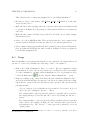
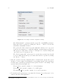
A.3 Usage . . . . . . . . . . . . . . . . . . . . . . . . . . . . . . . . . . . . . . . .
56
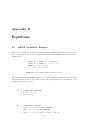
B Equations
59
B.1 mlBNF Modularity Example . . . . . . . . . . . . . . . . . . . . . . . . . . .
59
B.2 Another Modularity Example . . . . . . . . . . . . . . . . . . . . . . . . . . .
60
C mlBNF Mapping
62
C.1 mlBNF Abstract Syntax . . . . . . . . . . . . . . . . . . . . . . . . . . . . . .
63
C.2 Annotated mlBNF Concrete Syntax . . . . . . . . . . . . . . . . . . . . . . .
63
C.3 Pico.rmalbnf . . . . . . . . . . . . . . . . . . . . . . . . . . . . . . . . . . . .
67
C.4 Pico.xml . . . . . . . . . . . . . . . . . . . . . . . . . . . . . . . . . . . . . . .
68
D Generated Parser Example
69
D.1 Test.rmalbnf . . . . . . . . . . . . . . . . . . . . . . . . . . . . . . . . . . . .
69
D.2 Lex Test.java . . . . . . . . . . . . . . . . . . . . . . . . . . . . . . . . . . . .
70
D.3 Parse Test.java . . . . . . . . . . . . . . . . . . . . . . . . . . . . . . . . . . .
71
Bibliography
83
v
List of Figures
2.1
An example of an SPPF. Rounded rectangles are symbol nodes, rectangles are
intermediate nodes and circles are packed nodes . . . . . . . . . . . . . . . . .
5
An example of a meta-model, depicting how meta-models are depicted throughout this thesis. . . . . . . . . . . . . . . . . . . . . . . . . . . . . . . . . . . .
6
2.3
Another example of the same model . . . . . . . . . . . . . . . . . . . . . . .
7
2.4
Simplified Ecore meta-model . . . . . . . . . . . . . . . . . . . . . . . . . . .
8
2.5
Simplified meta-model of Ecore package structure . . . . . . . . . . . . . . . .
9
4.1
Small meta-model for a declaration . . . . . . . . . . . . . . . . . . . . . . . .
21
5.1
Overview of the architecture . . . . . . . . . . . . . . . . . . . . . . . . . . . .
23
5.2
An example of an IPFR (b) for input string "abc" given the grammar in (a).
Ambiguity node A has two production node children . . . . . . . . . . . . . .
25
An annotated IPFR. The annotations of the production nodes are placed below
the production nodes . . . . . . . . . . . . . . . . . . . . . . . . . . . . . . . .
27
An example of the current disambiguation mechanism. The left first (left) child
of each ambiguous node is chosen . . . . . . . . . . . . . . . . . . . . . . . . .
28
5.5
A simplified meta-model of a Java class . . . . . . . . . . . . . . . . . . . . .
29
6.1
Import graph . . . . . . . . . . . . . . . . . . . . . . . . . . . . . . . . . . . .
32
6.2
The object model for ALBNF syntax definitions
. . . . . . . . . . . . . . . .
33
6.3
An example of unused production rules. The production rules for <String+>
and <String> can not be reached from <Start> . . . . . . . . . . . . . . . .
34
An example of a grammar to indicate how grammar slots are stored internally
in SPPF nodes . . . . . . . . . . . . . . . . . . . . . . . . . . . . . . . . . . .
37
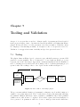
7.1
The workflow of the Eclipse plug-in . . . . . . . . . . . . . . . . . . . . . . . .
42
7.2
The workflow of the generated model generator . . . . . . . . . . . . . . . . .
43
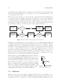
7.3
An example of project relative imports . . . . . . . . . . . . . . . . . . . . . .
43
2.2
5.3
5.4
6.4
vi
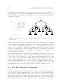
8.1
An example of a context free grammar (a) which leads to an ambiguous derivation for "1+2+3"(b) . . . . . . . . . . . . . . . . . . . . . . . . . . . . . . . . .
49
EClass A is referencing EClass B using a non-containment reference . . . . .
51
A.1 How to import a project . . . . . . . . . . . . . . . . . . . . . . . . . . . . . .
54
A.2 An example of a project setup . . . . . . . . . . . . . . . . . . . . . . . . . . .
55
A.3 An example of launch configuration settings . . . . . . . . . . . . . . . . . . .
57
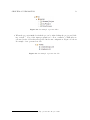
A.4 An example of generated files . . . . . . . . . . . . . . . . . . . . . . . . . . .
58
A.5 An example of generated models . . . . . . . . . . . . . . . . . . . . . . . . .
58
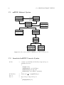
C.1 A workflow of the model generation process . . . . . . . . . . . . . . . . . . .
62
C.2 The abstract syntax of mlBNF in the form of a meta-model . . . . . . . . . .
63
C.3 An example of a model generated from the mlBNF definition in Section C.3 .
68
9.1
vii
List of Tables
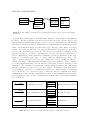
2.1
An overview of meta-model symbols that occur in this document . . . . . . .
6
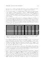
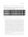
7.1
Metrics for grammars, meta-models and GLL parsers for the languages ALBNF,
mlBNF, two implementations of Pico, iDSL, Oberon and Ansi C . . . . . . .
44
Metrics for generated parsers for two implementations of Pico, iDSL, Oberon
and Ansi C . . . . . . . . . . . . . . . . . . . . . . . . . . . . . . . . . . . . .
45
7.2
viii
List of Listings
2.1
2.2
An example of a part of a context free grammar in BNF . . . . . . . . . . . .
An example of a model . . . . . . . . . . . . . . . . . . . . . . . . . . . . . . .
4
7
4.1
4.2
A representation of the Annotated-Labeled-BNF formalism . . . . . . . . . . .
The mlBNF formalism is an extension of the ALBNF formalism which was
specified in Figure 4.1 . . . . . . . . . . . . . . . . . . . . . . . . . . . . . . .
Module A should be able to reference B’s production rules, but not vice versa
An example to illustrate the modularity normalization . . . . . . . . . . . . .
Small example of an ALBNF syntax definition using annotations to specify a
mapping to a meta-model . . . . . . . . . . . . . . . . . . . . . . . . . . . . .
16
18
19
20
5.1
5.2
An example ALBNF grammar for which a parser is generated . . . . . . . . .
A Java program . . . . . . . . . . . . . . . . . . . . . . . . . . . . . . . . . . .
24
29
6.1
6.2
A typical example of parser generation code . . . . . . . . . . . . . . . . . . .
A typical example of model generation code . . . . . . . . . . . . . . . . . . .
35
39
B.1 A modularity example with three modules . . . . . . . . . . . . . . . . . . . .
B.2 A modularity example with five modules . . . . . . . . . . . . . . . . . . . . .
59
60
4.3
4.4
4.5
ix
20
Chapter 1
Introduction
The design of domain specific languages (DSLs) is influenced by many factors. Mauw et.al.
[21] describe the steps needed to develop an effective DSL, perhaps the most important of
which is domain analysis (a form of requirements engineering) since this step is the primary
influence of the choice of language constructs to be integrated into the new language. In this
thesis, we focus on the technical aspects associated with the design of a DSL. We consider,
as described in Kleppe [17] the abstract syntax to be the most important ingredient in DSL
design. This is mainly because the abstract syntax definition (or meta-model) is the starting
point for defining the (static) semantics of the DSL and the textual or graphical concrete
syntax.
The focus of this thesis will be on the creation of textual concrete syntaxes for a given arbitrary
abstract syntax/meta-model. In order to make the abstract syntax drive the development of
a DSL it is very important to have as few restrictions as possible, which currently many tools
such as Xtext [10] or EMFText [8] enforce, on the specification of abstract syntax for the DSLs
that are created, or on the class of accepted context free grammars. We will use a Generalized
LL parsing algorithm as our starting point [25]. This means that we do not have to restrict
ourselves to the LL(k) class of grammars. We have developed a parser generator in Java
that generates Java GLL parsers. These GLL parsers parse input sentences and construct
models that represent the corresponding abstract syntax trees; the models are constructed
via calls to the constructors which reference predefined meta-models. We propose a modular
annotated grammar formalism. The modularity presents two axes: we can import more than
one meta-model and we can split our concrete syntax definition into separate modules.
It is of course important to consider the contribution of the research presented in this document to current environments in which DSLs are emplyed. For situations in which DSLs based
on meta-models have been used for a certain period the research presented in this document
is indeed useful. For example, companies which have been developing DSLs to support their
industrial processes now struggle with problems related to new developments in DSL technologies and environments. Ideally, they would like to incorporate the existing technologies
into a single development environment without redeveloping all the existing DSLs. Our approach is aimed at generating languages for existing meta-models and is therefore suitable for
creating new concrete syntax for existing DSLs without changing the framework behind the
DSL, as was described by Thomas Delissen in his master’s thesis[6]. In order to increase the
1
CHAPTER 1. INTRODUCTION
2
(re)-usability of language specifications, modular concrete syntax specifications and abstract
syntax specifications can be employed.
In order to create a usable concrete syntax formalism in combination with GLL parsing, we
have to answer the following two questions:
1. What is needed in a concrete syntax formalism to define a mapping from the concrete
syntax of a domain specific language to a pre-existing abstract syntax specification?
2. Is GLL applicable in an environment in which input strings conforming to a given
concrete syntax have to be mapped to an abstract syntax representation?
In this thesis we try to answer these two questions.
The layout of this thesis is as follows. Chapter 2 gives background information about topics
that are considered important to understand the work described in this thesis. Chapter 3
gives a short list of research that has been done in the same area as the work that is described
in this thesis. In the next chapter, Chapter 4, a formalism for defining context free grammars
is defined. This modular formalism is based on BNF and contains annotations to define a
mapping from the concrete syntax to meta-models. Chapter 5 explains how abstract syntax
can be defined using this mapping. In order to test the method that is proposed in this
thesis the described aspects are implemented. An overview of the implementation is given
in Chapter 6. To check whether the implementation and the methodology described in this
thesis are usable, a tool has been created and some tests have been performed using this tool.
Both the tool and the tests are described in Chapter 7. The rest of the thesis contains a
discussion about future research that can be performed on this topic (Chapter 8) and some
known but unresolved issues in the implementation of the tool (Chapter 9). Conclusions
about the research are given in Chapter 10.
Chapter 2
Preliminaries
In this chapter topics that are considered important for the rest of this thesis are briefly
explained. The purpose of this chapter is not to be extensive and complete, but to mention
and explain concepts which are often referred to throughout this thesis. To satisfy readers
who want to know more about specific topics, pointers to more extensive resources are given.
The topics that are treated in this chapter are parsing and meta-modeling. In the section
about parsing (Section 2.1) context free grammars, parsers and parsing algorithms are described. An important part of this chapter will be devoted to GLL Parsing (Section 2.2),
because this is the parsing technique that is used for our research. Meta-modeling is explained briefly in Section 2.3 and a specific implementation of meta-modeling, called the
Eclipse Modeling Framework is described in Section 2.4.
2.1
Parsing
Parsing, or syntax analysis is the process by which the grammatical structure of a text is
determined. This is in contrast to lexical analysis, in which an input string is divided into a
number of tokens. Parsing is used in many applications. Typically, parsers (i.e. tools that
preform parsing) are generated from a human readable language.
A context free grammar (CFG), see [1] Section 4.2, consists of a set of nonterminals, a set
of terminals, a set of derivation rules of the form A ::= α where the left hand side A is a
nonterminal, and the right hand side α is a string containing both terminals and nonterminals,
or consisting of the empty symbol . Every CFG has a specified start symbol, S, which is
a nonterminal. Rules with the same left hand side can be written as a single rule using the
alternation symbol, A ::= α1 | . . . | αt . The strings αj are called the alternates of A.
Listing 2.1 shows an example of a context free grammar in Backus-Naur Form (BNF). In
this example emphasized tokens, like <Program>, <Declarations> or <Statements> are
nonterminals and tokens enclosed in apostrophes like "begin", ";" or "end" are terminals.
By convention, the first defined symbol, in this case <Program>, is used as the start symbol.
The production rule for <Statements> contains the symbol, indicating that <Statements>
can derive the empty string.
3
CHAPTER 2. PRELIMINARIES
<Program>
<Declarations>
<Declaration>
<Id >
<Type>
<Statements>
::=
::=
|
::=
::=
::=
|
::=
|
4
"begin" <Declarations> ";" <Statements> "end"
<Declaration>
<Declaration> "," <Declarations>
<Id > ":" <Type>
[A-Z][A-Za-z0-9 ]+
"natural"
"string"
<Statement> ";" <Statements>
Listing 2.1: An example of a part of a context free grammar in BNF
A grammar Γ defines a set of strings of terminals, its language, as follows. A derivation
step, has the form γAβ⇒γαβ where γ and β are both lists of terminals and nonterminals and
A ::= α is a grammar rule. A derivation of τ from σ is a sequence σ⇒β1 ⇒β2 ⇒ . . . ⇒βn−1 ⇒τ ,
∗
also written σ ⇒τ . A derivation is left-most if at each step the left-most nonterminal is
∗
replaced. The language defined by Γ is the set of u ∈ T∗ such that S ⇒u.
∗
The role of a parser for Γ is, given a string u ∈ T∗ , to find (all) the derivations S ⇒u.
Typically, these derivations will be recorded as trees. A derivation tree in Γ is an ordered
tree whose root node is labeled with the start symbol, whose interior nodes are labeled with
nonterminals and whose leaf nodes are labeled with elements of T ∪ {}. The children of a
node labeled A are ordered and labeled with the symbols, in order, from an alternate of A.
The yield of the tree is the string of leaf node labels in left to right order.
Over the years, many parsing algorithms have been developed. Within the world of parsing,
there are two main movements, top-down parsing and bottom-up parsing (see [1], Chapter 4).
Both parsing strategies are used to construct a derivation of an input string given a grammar.
The difference is that in top-down parsing the derivation starts with the start symbol and
nonterminals are expanded by substituting left hand sides with their right hand sides until
the input string appears. In bottom-up parsing, the derivation starts with the input string
and right hand sides of production rules are substituted by their left hand sides until the
start symbol is derived. The standard parsing techniques are useful when the input language
complies to a number of restrictions and the full set of context free languages can not totaly
be parsed using conventional parsers.
To be able to parse input strings in these languages, more powerful parsing algorithms have to
be used. For both top-down parsing and bottom-up parsing techniques generalized parsers[20,
28] have been invented. These parsers do not return parse trees as the result of a parse, but
a parse forest. A parse forest is, in a way, a generalization of a parse tree. A parse forest
consists of a number of parse trees, each corresponding to a derivation of the input string. In
some cases, parse forest can even contain cyclic paths. So unfortunately, the extra power of
generalized parsing techniques comes with extra difficulties. For example, in most applications
only on parse tree is preferred, this means that the parse forest has to be pruned. Incorrect
parse trees have to be removed. Often, this can not be done at parse time, but only after the
entire parse forest is generated.
5
2.2
2.3. GLL PARSING
GLL Parsing
Generalized LL parsing, or GLL parsing[25, 24], is a kind of generalized top-down parsing.
A GLL parser traverses an input string and returns all possible derivations of that string.
Internally, a GLL parser constructs a Tomita style graph structured stack (GSS)[29]. This
GSS is used to keep track of the different traversal threads which arise when an input string
is traversed. Multiple traversal threads are handled using process descriptors. These process
descriptors make the algorithm parallel in nature. Each time a traversal bifurcates, the current
grammar and input positions, together with the top of the current stack and associated
portion of the derivation tree, are recorded in a descriptor. The created descriptors are
stored and at every cycle of the parser one descriptor is removed and the parser continues the
traversal thread from the point at which the descriptor was created. When the set of pending
descriptors is empty all possible traversals have been explored and all derivations (if there are
any) have been found.
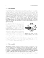
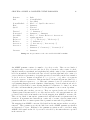
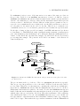
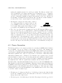
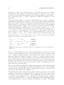
The output of a GLL parser is a representation of all
S, 0, 3
the possible derivations of the input in the form of a
binarised shared packed parse forest (SPPF), which is
a union of all the derivation trees of the input string.
A binarised SPPF has three types of nodes: symbol
S ::= ab ∙ c, 0, 2
A, 1, 3
nodes, with labels of the form (x, i, j) where x is a
terminal, nonterminal or and 0 ≤ i ≤ j ≤ n, where
a, 0, 1
c, 2, 3
n is the length of the input string; intermediate nodes,
b, 1, 2
with labels of the form (t, i, j) used for the binarisation
of the SPPF and allowing for a cubic runtime bound
on GLL parses; and packed nodes, with labels of the
Figure 2.1: An example of an SPPF.
form (t, k), where 0 ≤ k ≤ n and t is a grammar slot.
Rounded rectangles are symbol nodes,
Terminal symbol nodes have no children. Nonterminal rectangles are intermediate nodes and
symbol nodes, (A, i, j), have packed node children of circles are packed nodes
the form (A ::= γ·, k) and intermediate nodes, (t, i, j),
have packed node children with labels of the form (t, k), where i ≤ k ≤ j. A packed node has
one or two children, the right child is a symbol node (x, k, j), and the left child, if it exists,
is a symbol or intermediate node, (s, i, k). For example, for the grammar S ::= abc | aA,
A ::= bc we obtain the SPPF as shown in Figure 2.1.
2.3
Meta-models
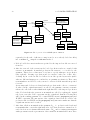
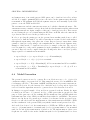
Throughout this thesis, the terms meta-model and model will be used frequently. A metamodel is a collection of concepts which have properties and which can be related to each other.
A model is an instantiation of a certain meta-model, it is said that a model corresponds to
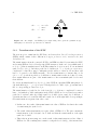
its meta-model. In meta-modeling terms, a meta-model is an instantiation of a meta-metamodel. Figure 2.2 shows a meta-model in the way meta-models are depicted throughout this
document. For the sake of clarity, this example meta-model will be explained briefly.
The meta-model contains four concepts, “AbstractObject”, “Object”, “Attribute” and “Type”.
Concepts are sometimes referred to as classes. The concept “AbstractObject” is an abstract
CHAPTER 2. PRELIMINARIES
AbstractObject
6
Object
+name : String
attributes
0..*
1
Attribute
+name : String
+value : String
+type : Type
«enumeration»
Type
+Integer
+String
+Real
baseObject
Figure 2.2: An example of a meta-model, depicting how meta-models are depicted throughout
this thesis.
concept (indicated in the figure by its italics name). Abstract concepts cannot be instantiated
in a model. The arrow with the open-ended arrow head between the concepts “Object” and
“AbstractObject” indicates that “Object” is a sub concept of “AbstractObject” which means
that “Object” has all properties of “AbstractObject”, which in this case means the property
“name”. As shown in the figure, properties have types. The type of the “name” property is
“String”. Properties can also have concept types (these kind of properties are often called
references, the other kind op properties are also referred to as attributes). Examples are the
property “baseObject” of “Object” which has type “Object”, the property “attributes” of
“Object” which has a possible empty list of “Attribute”s as its type (indicated by the cardinality “0..*”) and the property “type” of concept “Attribute” which has type “Type”. The
“Type” concept is called an enumeration and contains a list of literals, in this case “Integer”,
“String” and “Real”. This means that instantiated properties with type “Type” can have
one of these literals as its value. Note the difference between the references “baseObject” and
“attributes”. The “attributes” reference has a diamond shaped starting point. This means
that the “attributes” reference is a containment relation. In instances of the meta-model,
concepts that are referenced by containment references are contained in the concepts that
refer to them. For non-containment references this is not the case. Attributes are always
containment properties. Listing 2.2 and Figure 2.3 show possible instantiations of the metamodel in Figure 2.2. An overview of all meta-model elements that occur in this document is
given in Table 2.1.
name
cardinality
Name
Containment relation
Abstract meta-model class
Name
name
cardinality
Non-containment relation
Meta-model class
«enumeration»
Name
Aggregation relation
0..∗
Zero or more cardinality
Enumeration
1
Exactly one cardinality
Table 2.1: An overview of meta-model symbols that occur in this document
7
2.4. ECLIPSE MODELING FRAMEWORK
<Object name="BaseObject">
<attribute name="atr1" value="test" type="Type.String"/>
<attribute name="atr2" value="100" type="Type.Integer"/>
<attribute name="atr3" value="1.05" type="Type.Real"/>
</Object>
<Object name="SubObject">
<baseObject id="BaseObject">
<attribute name="attr4" value="test" type="Type.String"/>
</Object>
Listing 2.2: An example of a model. This model is an instantiation of the meta-model in Figure
2.2
As shown in Listing 2.2 and Figure 2.3, there are
BaseObject
two instances of the “Object” concept, namely one
- atr1: String = “test”
named BaseObject and one named SubObject. Both
- atr2: Integer = 100
instances have instances of “Attribute” concepts in
- atr3: Real = 1.05
them, this is because the containment reference that
exists between the “Object” and “Attribute” classes
SubObject
in the meta-model. The instantiation SubObject con- atr4: String = “test”
tains also a reference to the instantiation BaseObject.
Because the “baseObject” reference of the “Object”
concept is a non-containment reference in the meta- Figure 2.3: Another example of the
model, the instantiation BaseObject is not contained same model
in the instantiation SubObject.
2.4
Eclipse Modeling Framework
The Meta-Object Facility (MOF)[11] is an initiative to describe meta-models, initially used
for describing UML diagrams using a four-layered architecture. MOF, initially defined for
describing UML diagrams, is a four-layered architecture. The top layer Meta-Meta-Model
Layer (M3) defines the structure of the meta-metadata. The elements on this layer are
described in terms of themselves, much as the syntax of BNF may be defined using BNF
itself. The second layer Meta-Model Layer (M2) defines the structure of the metadata. The
elements of the M3 layer are used to build meta-models. Just as, for example, BNF can be
used to describe the syntax of Java, the model elements of M3 can be used to define the
meta-models of the individual UML diagrams. The third layer Model Layer (M1) describes
the models themselves. This layer uses the elements of the M2 layer to define UML models,
just as the Java grammar defines legal Java programs. The fourth layer Data Layer (M0)
describes objects or data that are being manipulated.
The Eclipse Modeling Framework (EMF)[27] provides a meta-meta-model which can be used
to define any meta-model. It provides classes, attributes, relationships, data types, etc.
and is referred to as Ecore. MOF is essentially a definition, whereas Ecore is a concrete
implementation of MOF in Eclipse. Ecore is mainly used to facilitate the definition of domain
specific languages and it is used to define their meta-models. These meta-models essentially
CHAPTER 2. PRELIMINARIES
8
describe the abstract syntax of the domain specific language.
We use EMF and Ecore to define meta-models. Although meta-models and abstract syntax
are not exactly the same, we will use the terms interchangeably here. A meta-model can
represent an abstract syntax but with extra information, for instance the attributes in the
classes can be used to store type information, or links between identifiers can be established
in a meta-model. More information on the similarities and differences between meta-models
and abstract syntax trees can be found in Alanen and Porres [2], Kleppe [16], and Kunert
[19].
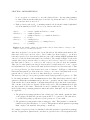
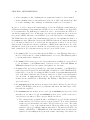
Abstract syntax in the form of a meta-model subsumes several important notions. Figure 2.4
shows a simplified version of the Ecore meta-meta-model. EClass models the classes which
are identified by a name and may have a number of attributes and a number of references.
EAttribute models the attributes which are also identified by a name and a type. EDataType
represents the simple types, corresponding to the Java primitive types and Java object types.
EReference models the associations between classes. An EReference is identified by a name
and it has a type which must be an EClass. Furthermore, it has a containment attribute
indicating whether the EReference is used as whole-part relationship. Within ECore, both
EAttributes and EReferences are referred to as structural features.
eAttributes
0..*
EAttribute
eAttributeType
+name : String
EDataType
1
EClass
+name : String
eReferences
1
0..*
eReferenceType
EReference
+name : String
+containment : boolean
Figure 2.4: Simplified Ecore meta-model
2.4.1
Modularity in Ecore
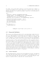
In Ecore, related classes and types can be grouped into so called packages, which are modeled
by Ecore’s EPackages (Figure 2.5 shows a meta-model that represents the package and related
concepts). The eClassifiers reference contains all the classes and types that are present in
an EPackage (EClassifier is the super type of EClass and EDataType in Ecore). EPackages
have three attributes, name, nsURI and nsPrefix. The name attribute does not have to be
unique, because the nsURI attribute is used to uniquely identify an EPackage. The nsPrefix
attribute reflects Ecore’s close relationship to XML and it is used as an XML namespace if an
Ecore model is serialized to XML. The modularity of Ecore is reflected by the eSuperPackage
reference and the eSubPackages reference. The eSubPackages reference contains all EPackages
on which an EPackage depends, classes and types that are defined in the EPackages that are
contained in eSubPackages can be used in the containing EPackage. Every EPackage can only
be contained in one other EPackage. This containment is indicated by the eSuperPackage
9
2.4. ECLIPSE MODELING FRAMEWORK
reference.
EClassifier
EFactory
0..*
eClassifiers
eSubPackages
EPackage
+nsURI : String
+nsPrefix : String
+name
1
eFactoryInstance
+create()
+createFromString()
+convertToString()
0..*
eSuperPackage
Figure 2.5: Simplified meta-model of Ecore package structure
Within Ecore, for every EPackage an EFactory exists and can be obtained using the eFactoryInstance reference. EFactories are used to (reflectively) generate instances of the metamodel that is defined in an EPackage. The create method that is defined for EFactories are
used to create model elements such as EClasses, EReferences or EAttributes. The other two
methods, createFromString and convertToString are used to respectively create and convert
EDataTypes from and to strings.
Chapter 3
Related Work
In this section research and projects that are related to this project are described. We have
chosen a number of so-called language development frameworks (LDFs), basically tools which
can be used for the creation of development environments for languages, and explain what
they do and how they compare to our approach.
We have chosen five different examples of LDFs. The Meta-Environment (Section 3.1), which
is an early example of a language development framework uses SDF for defining the concrete
grammar of a language. Spoofax/IMP (Section 3.2) is based on the Eclipse development
platform and also uses SDF [32] for the definition of languages. Xtext and EMFText (Sections 3.3 and 3.4 respectively) are other LDFs based on the Eclipse platform. All these LDFs
uses parsers to transform instances of DSLs into abstract syntax definitions. MPS, Section 3.5
is a LDF which does not depend on parser generation, but is based on editing the abstract
syntax directly without the intervention of a parser.
3.1
ASF+SDF Meta-Environment
The ASF+SDF Meta-Environment, or simply the Meta-Environment[18, 31] was one of the
first language workbenches. It uses the combination of the Algebraic Specification Formalism(ASF)[3] to describe semantics of DSLs and the Syntax Definition Formalism(SDF)[12]
to describe the syntax of DSLs. Within the ASF+SDF Meta-Environment it is possible to
generate editors for DSLs using a combination of ASF and SDF, called ASF+SDF.
The latest version of the ASF+SDF Meta-Environment uses SDF2[32] instead of SDF. SDF2
is a modular syntax formalism based on SDF. The modules in SDF2 consist of a number of
sections, including a context free syntax section, in which context free production rules are
defined and a lexical syntax section in which lexical production rules are defined. SDF2 also
has a number of disambiguation constructs, for example: priorities which define priorities
between production rules and associativity indicators which indicate how the associativity of
operators is defined.
The Meta-Environment uses a bottom-up parser, called SGLR (for scanner-less generalized
LR). The disambiguation constructs defined in the SDF2 syntax are needed because of the
generalized parsing approach. The Meta-Environment uses the ATerms library[30] to repre10
11
3.3. SPOOFAX/IMP
sent the abstract syntax of defined languages.
Because the ASF+SDF Meta-Environment is one of the first language workbenches, it misses
many features that are present in more recent language workbenches. For example, things like
editor support or real-time parsing are not present in the editors that are generated by the
ASF+SDF Meta-Environment. However, the Meta-Environment has influenced more recent
LDFs. Spoofax/IMP (Section 3.2) also uses SDF2 as its concrete syntax definition formalism.
3.2
Spoofax/IMP
Spoofax/IMP, or simply Spoofax [15] is a language workbench based on the Eclipse IDE and
is aimed at the development of textual domain specific languages. Spoofax uses IMP[5], an
IDE meta-tooling for Eclipse, for the integration whith Eclipse. Within Spoofax, a language
definition consists of three main components.
1. The syntax of a DSL is defined in SDF2, this means that Spoofax supports complex
modular language definitions and has many disambiguation mechanisms built-in (see
also Section 3.1).
2. Service descriptors define how the behavior of generated editors is implemented.
3. The semantics of a DSL are defined using Stratego[4] which can be used for code
generation, etc.
In Spoofax, the grammar which is used to generate parsers contains both the concrete syntax
and the abstract syntax of the DSL for which the parser is generated. Inside Spoofax, the
abstract syntax which is contained in the SDF definitions is transformed into a set of firstorder terms, which are stored as Java objects. Spoofax uses an implementation of an SGLR
parser (a scanner-less generalized LR parser) for Java, called JSGLR[14] to create instances
of the abstract syntax of a DSL for programs written in that DSL.
As with our approach, Spoofax uses a generalized parsing technique. The difference with
our technique is that SGLR is a bottom-up parsing approach, whereas GLL uses a top-down
parsing approach. A similarity is that Spoofax and our approach both have modular syntax
definitions. Spoofax, as is the case with the ASF+SDF Meta-Environment, does not use
Ecore to represent the abstract syntax of DSLs. This means that the tooling based on Ecore
can not be exploited by Spoofax, thus all the functionality that is offered by these tools has to
be implemented for Spoofax’s abstract syntax representation. Our approach does use Ecore
to represent abstract syntax, thus we can benefit from the available Ecore tooling.
3.3
Xtext
Xtext[9, 10] is a so-called language development framework based on the Eclipse development
environment. This means that Xtext can be used to create support for DSLs in the Eclipse
IDE. Initially, Xtext was developed as part of the openArchitectureWare framework [22].
Later, it evolved to be a part of the Eclipse Textual Modeling Framework project (TMF).
CHAPTER 3. RELATED WORK
12
Xtext uses the ANTLR[23] parser generator for parsing Xtext grammars. ANTLR is an LL(*)
parser generator with a possibility for backtracking.
In an Xtext syntax specification the concrete syntax, which is expressed as a context free
grammar is interwoven with the abstract syntax. When generating parsers and so on using
the Xtext specification, from the abstract syntax definition an Ecore meta-model is generated.
Using the generated artifacts (parser, meta-model, etc.), Xtext is capable of generating editors for the language that was expressed in the original grammar specification. The generated
editors support a large number of features, including: syntax highlighting, code completion,
folding and bracket matching. Xtext is also capable of generating a concrete syntax outline from a meta-model. Developers can extend this outline with their own concrete syntax
constructs. This feature however, is not well documented and we assume that it is an experimental feature.
The approach of Xtext concerning the definition of the abstract syntax differs from our
approach in that it does not assume the abstract syntax to be a given. This means that
every time a DSL is created a new meta-model is generated for this DSL. In a scenario that
there already exists a language which has tooling support based on the meta-model for this
DSL and which has to be incorporated into a new environment, Xtext’s approach is not
desirable, because the tooling might have to be rewritten.
3.4
EMFText
EMFText[8] was initially developed as part of the Ruseware Composition Framework [7] at
Dresden University of Technology. Over time, it became available as an Eclipse plug-in. As
opposed to Xtext, EMFText allows specifying a concrete syntax for existing Ecore models.
Another difference is that Xtext does not allow for modular grammar specifications, whereas
EMFText does.
A concrete syntax specification in EMFText consist of three sections:
• A configuration section, containing the language name, the meta-model which defines
the abstract syntax and the class in the meta-model that defines the root of the abstract
syntax tree.
• A token section in which lexical tokens can be specified.
• A rules section where the concrete syntax for each class in the meta-model is defined.
A similarity between EMFText and Xtext is that they both use the ANTLR parser generator
to generate their parsers, this means that EMFText suffers the same restrictions for grammar
specifications as Xtext.
There are many similarities between EMFText’s approach and our approach. Both assume an
Ecore model to be given and both allow for modular syntax specifications. The main difference
is the parser technology that is used. Our GLL parsers are more powerful than EMFText’s
ANTLR parsers, which means that we have no restrictions on our grammar specifications.
13
3.6. MPS
3.5
MPS
MPS, which is an abbreviation for Meta Programming System[26] is another language development framework and is created by JetBrains [13]. In contrast to the before mentioned
language workbenches which are based on parser generation, MPS is a projectional editor.
This means that MPS follows the language oriented programming approach as described by
Sergey Dmitriev in [26] which eliminates the need of parser generation by editing an AST
indirectly.
The language oriented approach originated from the observation that plain text is not suitable
for storing programs. According to Dmitriev, plain text is not suitable because it does not
correspond to the abstract syntax trees that are used by compilers or interpreters (this explains
the need of parser generation in the before mentioned language workbenches) and that it is
therefore hard to extend textual languages because each extension increases the possibility of
ambiguities in the language. The language oriented approach separates the representation of
a language from its storage, which means that programs can be stored as structured graphs
that can directly be used by compilers and so on.
In order to separate representation of a language from its storage, in the language oriented
approach the definition of a DSL is separated in three parts.
1. The so-called structure defines the abstract syntax of the language and is represented
by concepts. Concepts define the properties of elements in the abstract syntax in a way
similar to meta-models. The structure on an MPS language is defined in the structure
language.
2. Editors are used to support the concrete syntax of an language. In MPS, editors are
defined using the editor language.
3. In order to make a language defined in MPS functional the semantics of a language
are expressed in the transformation language. The transformation language is used for
defining model transformations.
The main difference between MPS and the approach that is proposed in this thesis is the lack
of parsers to create abstract syntax trees for DSLs. The problem that it is hard to assign a
semantics to an ambiguous language, which is the basis of the language oriented approach
as used in MPS can be solved in our approach by defining disambiguation constructs in the
language that is used in the generation of parsers in a way similar to SDF (see Section 3.1).
3.6
Conclusions
As described in this chapter, there already exist many approaches for combining and mapping
concrete syntax of DSLs to abstract syntax. All these approaches however, have one or more
disadvantages. Most of the approaches described in this chapter can not be used with existing
abstract syntax specifications, which is a requirement of our approach. Another disadvantage
is that restrictive parser techniques are used, which is visible in the specification of concrete
syntaxes.
CHAPTER 3. RELATED WORK
14
A major difference between the approach that is described in this thesis and the approaches of
many existing language workbench tools is that in our approach abstract syntax trees or ASTs
are used to describe the abstract syntax of a DSL, whereas other tools use abstract syntax
graphs or ASGs to describe the abstract syntax. The use of ASGs enables static verification
of segments of a DSL (for example checking whether variables have been defined). However,
using model transformations can be used to transform an AST into an ASG, therefore we
consider the creation of ASGs as a separate step which is not present in described in this
thesis.
Chapter 4
mlBNF: A Concrete Syntax
Formalism
In the previous chapter we exposed some disadvantages of existing approaches. The most
important disadvantages are:
1. Existing meta-models can not directly be used as the abstract syntax of a DSL, and
2. Used parsing techniques are restrictive, so the concrete syntax definitions are subject
to these restrictions.
In order to solve these disadvantages we define a mapping from concrete syntax to abstract
syntax. We have developed a modular context free grammar formalism based on BNF within
which it is possible to express the mapping from grammar production rules to model objects
adhering to a predefined meta-model and their attributes and references. We start with
defining the grammar formalism. Section 4.1 gives an overview of the grammar formalism
and in Section 4.2 we describe how modules are added to this formalism. In Section 4.3 the
mapping from concrete syntax to abstract syntax that can be combined with the grammar
formalism is described.
4.1
Annotated-Labeled-BNF
In this section we describe a simple but effective BNF based context free grammar formalism
which forms the basis for a parser generator that is used to generate GLL parsers. The
formalism is called Annotated-Labeled-BNF (ALBNF) and consists of annotated production
rules. Listing 4.1 shows a simplified EBNF representation of the ALBNF formalism.
In ALBNF, BNF is extended with labeled nonterminals in the right hand sides of production
rules and with annotations for production rules. These annotations can be used for a number
of different purposes, e.g. to express disambiguation constructs, as was done in SDF2 [32],
or to express the mapping from concrete syntax to abstract syntax. It is the latter type of
annotations, in particular the mapping from ALBNF to meta-models, that are described in
this thesis.
15
CHAPTER 4. MLBNF: A CONCRETE SYNTAX FORMALISM
Grammar
Rule
ContextFreeRule
Head
Symbol
Terminal
Nonterminal
LexicalRule
Pattern
Exclusions?
Exclusion
Annotations
Annotation
Parameter
::=
::=
|
::=
::=
::=
|
::=
::=
::=
::=
::=
::=
::=
::=
|
::=
16
Rule∗
ContextFreeRule
LexicalRule
Head “::=” Symbol ∗ Annotations?
characters
Terminal
Nonterminal
“"” characters “"”
characters “:” characters
Head “::=” Pattern Exclusions? Annotations?
regular expression
“—
/ ” “{” Exclusion (“,” Exclusion)∗ “}”
“"” characters “"”
“{” Annotation (“,” Annotation)∗ “}”
characters
characters “(” Parameter (“,” Parameter )* “)”
characters
Listing 4.1: A representation of the Annotated-Labeled-BNF formalism
An ALBNF grammar consists of a number of production rules. There are two kinds of
production rules, context free rules and lexical rules. Context free rules consist of a head,
which is basically a nonterminal, and a right hand side which consist of a list of terminals and
labeled nonterminals. Lexical rules also have a head, but their right hand sides consist of a
pattern, which is a representation of a regular expression. Lexical rules can also have a number
of lexical exclusions. Assume a lexical rule L ::= α —
/ {e1 , e2 , . . . , en }, where α is a pattern
and ei is a sequence of characters. This means that L can match all patterns defined by α
except the character sequences e1 . . . en . This can for instance be used to exclude keywords of
a programming language from the identifiers of that language. Lexical exclusions can only be
expressed on lexical rules, because allowing this kind of exclusions to be defined on context
free rules could mean that the parser based on the grammar becomes context dependant.
Apart from this, rules can have annotations. These are expressed at the end of a rule as a
comma separated list surrounded by accolades and are used to add extra information to the
production rules, such as information used in the mapping from ALBNF to meta-models.
There are two kinds of annotations: parameterized annotations and non-parameterized annotations. Non-parameterized annotations consist only of a name, whereas parameterized
parameters also have a comma separated list of parameters surrounded by parentheses.
The mapping from ALBNF to meta-models defined in the annotations can have several parameters. These parameters specify the link between the ALBNF grammar specification
and meta-model objects. Elements of the grammar specification can be referenced using
ALBNF’s label names and model objects can be referenced by the names that were specified
in the meta-model.
17
4.2. ANNOTATED-LABELED-BNF
4.1.1
Lexical Patterns
So far, we have discussed the syntax of ALBNF, but we have not elaborated on how the regular
expressions of which the right hand sides of lexical production rules exist are represented. The
enumeration below gives an extensive overview of how these lexical patterns are constructed.
We start with defining character ranges and end with the definition for patterns, which are
basically the regular expressions that are mentioned in Listing 4.1. The patterns are used to
match a (part of a) string, what is matched by each pattern is also explained below.
• If a is a character then a is a range. a can be any character.
• If a and b are characters then a−b is a range. This range contains all characters enclosed
by and including a and b. There are two restriction on a and b: they are both of the
same type (digits, alphabetical characters or unicode characters for instance) and a is
lexicographically less than b.
• [] is a character class. This is a character class which contains no characters.
• If r1 . . . rn are ranges then [r1 . . . rn ] is a character class. This character class contains
all characters that are specified in the ranges ri .
• If r1 . . . rn are ranges then [∧r1 . . . rn ] is a character class. This is the negation character
class, it contains all all characters that are not specified in the ranges ri .
• If r1 . . . rn are ranges and q is a character class then [r1 . . . rn &&q] is a character class.
This is the intersection character class, it contains all characters that are specified in
the ranges ri that are also specified in q.
• If q is a character class then q is a pattern. This pattern matches the characters specified
in the character class q.
• If α is a pattern then α∗ is a pattern. The pattern α can be matched zero or more times
successively.
• If α is a pattern then α+ is a pattern. The pattern α can be matched one or more times
successively.
• If α is a pattern then α? is a pattern. The pattern α can be matched zero or one times.
• If α is a pattern then (α) is a pattern. The parentheses group patterns.
• If α and β are patterns then αβ is a pattern. The patterns α and β are concatenated.
So, first α is matched and then β is matched.
• If α and β are patterns then α|β is a pattern. Either α or β is matched.
Simple examples of patterns are: [a], which matches the character a, [a-z], which matches
exactly one alphabetic lowercase character, [a-zA-Z0-9], which matches exactly one alphabetic or numeric character and [0-9]+, which matches one or more numeric chacters. The
pattern ([a-z]|([A-Z][a-z]+))[0-9]? can match a0, Aa or Aa9 and more but not A or a91.
CHAPTER 4. MLBNF: A CONCRETE SYNTAX FORMALISM
4.2
18
mlBNF
Modularity is a often used abstraction technique in the field of software engineering. It enables
reusing software components, which decreases the development time of software products and
is often considered good practice. Most (if not all) popular programming paradigms support
one or more levels of modularity. The advantages of modularity can also be exploited in the
field of language specifications.
Therefore, a logical extension to ALBNF is the ability to split a grammar specification into
modules. Modules contain production rules and can import production rules from other
modules. It is also possible to retract production rules from imported modules. This means
that if in module m1 a production rule A ::= α is defined and another module m2 imports m1
and retracts A ::= α then A cannot derive α in m1 (except when a production A ::= α was
already present in m1 ). The retraction mechanism is an effective means of adjusting grammar
specifications according to specific requirements.
The usefulness of the retraction mechanism can be expressed by means of an example. Assume
that we intend to create parser for a version of Java which will be used in database applications
in which it is possible to express MySQL queries in strings. Ideally, we want to be able to parse
the MySQL strings, so that developers know whether their queries have the correct syntax.
To this extend, we could combine a Java grammar module and a MySQL grammar module.
The MySQL syntax however allows queries to be expressed on multiple lines, whereas Java
string can not cover multiple lines. Without altering the MySQL module directly, we can
retract the production rules which define the whitespace between query internals which allow
for the whitespace to span multiple lines. This example shows the usefulness of the retraction
mechanism, because it allows language developers to adapt modules to their specific needs
without altering these modules directly.
To distinguish between standard ALBNF and the modular version, we will refer to the later
as modular-labeled-BNF, or mlBNF. In Listing 4.2 an EBNF specification of the mlBNF
formalism is shown and in Appendix C.1 the abstract syntax of mlBNF is given by means of
a meta-model.
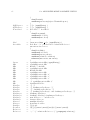
Module
ModuleName
Import
ModuleId
Retract
::=
::=
::=
::=
|
::=
“module” ModuleName Import∗ Grammar
characters
“import” ModuleId Retract∗
ModuleName
ModuleName “/” ModuleId
“retract” Rule
Listing 4.2: The mlBNF formalism is an extension of the ALBNF formalism which was specified
in Figure 4.1
The meaning of modularity in mlBNF can be expressed by means of a normalization function
|[·]|, which takes an mlBNF module and transforms it into a set or rules. The normalization
function is defined below.
Let N be the set of nonterminals, T be the set of terminals, M be the set of modules,
and R be the set of production rules. Furthermore, let name(m) denote the name of a
module for m ∈ M and let rules :: M → R∗ be the set of rules defined in a module. Let
19
4.2. MLBNF
imports :: M → (M × R∗ )∗ be the modules that are imported in a module joined with set
of retracted rules for each module, let module :: (M × R∗ ) → M return the module from an
imported module/retraction pair and let retract :: (M × R∗ ) → R∗ be the set of retracted
rules from a module/retraction pair. Let head :: R → N be the head of a production rule and
let expr :: R → h(N ∪ T)i be the tuple that forms the right hand side of a production rule.
Using these definitions we can define normalization rules for modules.
1. Let |[·]| :: M → R∗ be the normalization rule for a module. With m ∈ M, we define
|[m]| = |[imports(m)]| ∪ rules(m). The result of this normalization function is the set or
rules defined in m joined with the union of the normalization of the imported modules
of m and the rules defined in m
2. Let |[·]| :: (M × R∗ )∗ → R∗ be
S the normalization for a set of imported modules, if
∗
∗
∗
∗
ρm (rules(module(i))/retract(i)) ∪ {n ::= ρm (n)|n ∈
i ∈ (M × R ) then |[i ]| =
i∈i∗
N }, where m = name(module(i)) and N = {n|n = head(r) ∧ r ∈ rules(module(i))}.
The normalization of a set of imported modules consists of the union of the renamed
production rules (ρ is a renaming function and is defined below) of each imported module
in the set excluding the retracted production rules of each imported module. The
imported production rules are accessible in the importing module via the productions
{n ::= ρm (n)|n ∈ N }.
The function ρname is a renaming function which
renames production rules using the specified name.
module B
ρname is used to restrict the “visibility” of produc- module A
import
B
B ::= A
tion rules that are defined in different modules. ModA
::=
"1"
B
"3"
A ::= "2"
ules which are importing other modules should be able
to refer to nonterminals which are defined in the imported modules, but not vice versa. In the scenario Listing 4.3: Module A should be able
shown in Listing 4.3, module A should be able to ref- to reference B’s production rules, but not
erence the production rules B ::= A and A ::= "2" vice versa
defined in module B, but module B should not be able
to reference the production rule A ::= "1" B "3" defined in module A. A definition of ρ is
given below.
1. Let ρname :: R∗ →SR∗ be the renaming function for a set of rules. Now, if r∗ ∈ R∗
then ρname (r∗ ) =
ρname (r).
r∈r∗
2. Let ρname :: R → R be the renaming function for a single rule. Let r ∈ R, now
ρname (r) = ρname (head(r)) ::= ρname (expr(r)).
3. Let ρname :: h(N ∪ T)i → h(N ∪ T)i be the renaming function for the right hand side of
a production rule. Now with s ∈ h(T ∪ N)i, ρname (s) = hρname (s0 ) . . . ρname (s|s|−1 )i.
4. Let ρname :: N → N be the renaming function for a nonterminal. If n ∈ N, then
ρname (n) = name.n.
5. Let ρname :: T → T be the renaming function for a terminal. If t ∈ T, then ρname (t) =
t.
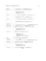
CHAPTER 4. MLBNF: A CONCRETE SYNTAX FORMALISM
module A
import B
import C
A ::= B C
module B
import C
B ::= "b.b"
C ::= "b.c"
20
module C
C ::= "c.c"
Listing 4.4: An example to illustrate the modularity normalization
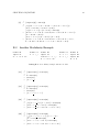
Assume that we have three production rules S::="a" B "c", S::="abc" and B::="b", applying the renaming function ρB to them leads to the production rules B.S::="a" B.B "c",
B.S::="abc" and B.B::="b". To illustrate the normalization function |[·]|, assume we have
three modules as shown in Table 4.4, of which module A is the main module. Now |[A]| =
{A ::= B C, B ::= B.B, B.B ::= "b.b", C ::= B.C, C ::= C.C, B.C ::= "b.c", B.C ::= C.C, C.C ::=
"c.c", C.C ::= B.C.C, B.C.C ::= "c.c"} See Appendix B.1 for the derivation of this result
and a larger (and more interesting) derivation.
4.3
Annotations for Mapping ALBNF to Meta-models
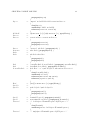
1. <Program>
2. <Declaration+>
3. <Declaration+>
4. <Declaration>
5. <Id >
6. <Type>
7. <Name? >
8. <Name? >
9. <Name>
::= <name:Name? > "begin" <decls:Declaration+> ";" "end"
{ class(Program), propagate(name),
{ reference(declarations, decls) }
::= <decl:Declaration>
{ propagate(decl) }
::= <decl:Declaration> "," <decls:Declaration+>
{ propagate(decl), propagate(decls) }
::= <id:Id > ":" <type:Type>
{ class(Declaration), attribute(name, id),
attribute(type, type) }
::= [a-zA-Z]+
{ type(EString) }
::= "natural"
{ enum(Type.Natural) }
::=
::= <name:Name>
{ attribute(name, name) }
::= [a-zA-Z]+
{ type(EString) }
Listing 4.5: Small example of an ALBNF syntax definition using annotations to specify a
mapping to a meta-model
Now the syntax of ALBNF and mlBNF is explained, we need to focus on the way in which the
mapping from concrete syntax to abstract syntax is defined. In order to define the mapping
from ALBNF to meta-model instances, we have established six kinds of annotations which
map directly to meta-model constructs. Figure 4.5 shows a small ALBNF example, extracted
from the syntax definition of a simple programming language. Figure 4.1 shows an example
21
4.3. ANNOTATIONS FOR MAPPING ALBNF TO META-MODELS
of a meta-model in which the abstract syntax of the ALBNF specification is defined. An
explanation of the supported annotations is given below.
• class(class-name): is used to indicate that the production rule for which this annotation is specified maps to a class instantiation in the generated model. The class-name
attribute indicates the name of the class to which the derivation corresponds. Production rule 4 in Listing 4.5 shows the usage of the class annotation for the creation of a
model class called “Declaration”.
• attribute(attribute-name, label ): indicates that value of the model attribute called
attribute-name of the previously created model class should be instantiated with the
result of the derivation of the nonterminal labeled label in the production rule for which
this annotation was specified. Listing 4.5 shows the attribute annotations for the
instantiation of the attributes “name” and “type” of the “Declaration” object with the
result of the derivation of the nonterminals labeled with “id” and “type” respectively.
• reference(reference-name, label ): indicates that value of the model reference called
reference-name of the previously created model class should be instantiated with the
result of the derivation of the nonterminal labeled label. The usage of the reference annotation is shown on line 1 in Listing 4.5. The usage is the same as the usage of the
attribute annotation.
Program
+name : String
Declaration
declarations
0..*
+name : String
+type : Type
«enumeration»
Type
+Natural
+String
Figure 4.1: Small meta-model for a declaration
• enum(enumeration-name.literal ): specifies that the production rule for which this annotation was specified contains a symbol that corresponds to an enumeration value in the
model. The enumeration-name.label parameter indicates the value of the enumeration
to which that symbol corresponds. An example of the usage of the enum annotation is shown in Listing 4.5, where for production rule 5 an enumeration value of type
“Type.Natural” is created.
• type(type-name): indicates that the yield of the parse forest for which this annotation
was defined should be mapped to a datatype called type-name. This can be a standard
datatype, like string or integer, but user defined datatypes are also allowed. Production
rule 5 in Listing 4.5 shows an example of the usage of the type annotation to create a
string representation for <Id >.
• propagate(label ): is used to indicate that the derivation of the grammar rule for which
this annotation is defined does not directly correspond to an instantiation of a metamodel construct, but that the derivation of a nonterminal labeled label, which is part of
the derivation of the grammar rule for which this annotation is specified is important
for the derivation. The usage of the propagate annotation is shown in production rule
3, where the mapping to a meta-model instantiation of <Declaration+> is split into
CHAPTER 4. MLBNF: A CONCRETE SYNTAX FORMALISM
22
the mapping for <Declaration> and <Declaration+> by means of this annotation type.
The combination of two propagate annotations allows for the creation of lists. In this
case, a list of <Declaration>s is created by means of the annotated production rules of
<Declaration+>. The propagate annotation can not only be used to construct lists,
it can, for example, also be used to instantiate optional attributes. This is shown in
line 1 in Listing 4.5. Here, <Name? > which is defined in lines 7 and 8, is propagated.
If no name is specified for a program, this will have no effect on the generated model.
If a name is specified however, the model will contain the name for the program, as is
specified in the attribute annotation in line 8.
4.4
Conclusions
In this section we have defined a new formalism for defining concrete syntax for domain specific
languages. This formalism, which we refer to as mlBNF, combines standard BNF constructs
with annotations that map the specified concrete syntax to a predefined abstract syntax. A
major advantage of mlBNF is that grammar specifications can be split into modules, because
this increases the usability and flexibility of grammar specifications. In Chapter 7 we describe
a tool that enables the use of mlBNF to generate models from program code and we validate
aspects of mlBNF.
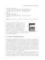
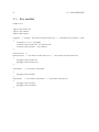
Chapter 5
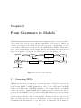
From Grammars to Models
An ALBNF grammar with annotations that define a mapping from the context free syntax to
a model is the basis of the process by which the particular model is generated. This process
consists of several steps, all of which depend on the generation or transformation of parse
forests. Firstly, a GLL parser is generated from the ALBNF syntax definition. This parser is
used to parse an input string, and the resulting SPPF is subsequently transformed and then
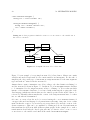
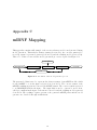
mapped to an instance of a meta-model. These steps are depicted in Figure 5.1.
conforms to
Metamodel
refers to
ALBNF
input for
Model
models
Parser Generator
generates
Input string
generates
Model Generator
input for
maps to
parses
GLL parser
IPFR
generates
SPPF
contains
Context free syntax
Figure 5.1: Overview of the architecture
5.1
Generating SPPFs
The first step in the model generation process is the generation of a GLL parser for a specific
language. As described in the previous chapter, for this purpose context free languages are
specified using ALBNF or mlBNF grammars. In order to create a GLL parser, an mlBNF
definition is normalized into an ALBNF grammar (i.e. the modular structure of an mlBNF
definition is reduced to a single ALBNF syntax definition, using the steps described in Section 4.2). Because ALBNF closely follows the standard BNF syntax, the process of generating
GLL parsers as described by Scott and Johnstone in [24] can be closely followed.
Generated parsers basically consist of a state machine containing a basic state, states for each
unique production rule head, states for each alternative of these heads and states for each
nonterminal in the right hand side of a production rule. To clarify this, look at Listing 5.1.
23
CHAPTER 5. FROM GRAMMARS TO MODELS
24
The GLL parser for this grammar has ten states, three arising from the nonterminals S, T
and U; two from the alternates of nonterminal T; two in total from the production rules for
nonterminals S and U and two from production rules S ::= t:T and T ::= "a" u:U which
both contain one nonterminal in their right hand sides and therefore both add one parser
state.
When a GLL parser parses an input string the state machine
is executed. The execution is guided by the tokens that are
S ::= t:T
identified by lexical analysis of the input string. In each state,
T ::= "a" "b" "c"
the GSS, which is the internal stack mechanism capable of repT ::= "a" u:U
resenting multiple stacks at the same time, and the SPPF are
U ::= "bc"
updated. A GLL parser succeeds when there exists a symbol
node (A, 0, n) in the SPPF, where A is the start symbol of the
Listing 5.1:
An example grammar and n is the length of the input string. If this is not
ALBNF grammar for which a the case after processing the entire input string the parser fails.
parser is generated
In our case, if the parse succeeds, the SPPF is transformed into
an IPFR, which is described in the next section.
5.2
The IPFR
The different notions that are shown in Figure 5.1 have been discussed in previous the chapters
of this thesis. The exception is the IPFR. The intermediate parse forest representation format,
is a simple way of representing parse forests. In comparison to the SPPF, it lacks information
about the position of symbols in the input string (this information is not needed during the
process of model generation) and can in many cases be used to compress the size of the forest
by means of maximal subterm sharing. In case of ambiguity, this format is often more efficient
to represent and to traverse. An IPFR contains three different kinds of nodes.
1. Terminal nodes (t) are nodes that represent or a terminal. In the later case t is the
lexeme of that terminal.
2. Production nodes contain a list of child nodes [s0 , . . . , sn−1 ]. Every sk is either a terminal node or an ambiguity node. Production nodes represent a specific derivation of a
nonterminal.
3. Ambiguity nodes (X) contain ambiguous derivations for the nonterminal X. It has a
list of child nodes [p0 , . . . , pn−1 ]. Every pk is a production node that represents a unique
derivation of X.
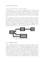
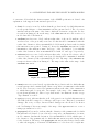
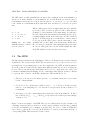
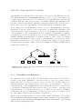
Figure 5.2 shows an example of an IPFR. There are two ambiguous nodes (the circular nodes
containing A and B), three production nodes (the empty circular nodes) and three terminal
nodes (the rectangular nodes containing a, bc and abc). In order to obtain an IPFR that
can be used to generate Ecore models, an SPPF has to be traversed and transformed into a
corresponding IPFR. This traversal is described next.
25
5.2. THE IPFR
A
<A>
<B >
::=
|
::=
"a" <B >
"abc"
"bc"
“a”
B
“abc”
“bc”
(a)
(b)
Figure 5.2: An example of an IPFR (b) for input string "abc" given the grammar in (a).
Ambiguity node A has two production node children
5.2.1
Transformation of the SPPF
The next step is to transform the SPPF into an Intermediate Parse Forest Representation
(IPFR), which consists of three different node types, production nodes, terminal nodes, and
ambiguity nodes.
The transformation from the generated SPPF to an IPFR is realized by traversing the SPPF
and creating IPFR nodes for several specific SPPF structures. In the case of a terminal symbol
node (t, i, j) this is straightforward: an IPFR terminal node (t) is created. For nonterminal
symbol nodes, (A, i, j), and their packed node children (A ::= α·, k) the process is more
complicated because there may be ambiguities in the subtrees of these nodes and these will
have to be passed to the IPFR structure. For the transformation of intermediate nodes
(A ::= α · β, i, j) and their packed node children no transformation rules are defined, because
these transformations are part of the transformation of the nonterminal symbol nodes and
their children.
For each nonterminal symbol node (A, i, j) of the SPPF an equivalent IPFR ambiguity node
(A) with children [p0 , . . . , pn−1 ]) is created. Each packed node child of (A, i, j) is transformed
into a corresponding production node pk .
The transformation of packed nodes of the form (A ::= α·, k) is more complicated because it
has to deal with the possible ambiguities in the SPPF. SPPFs are binarised and as a result a
packed node can have either (1) a single symbol node child, (2) two symbol node children, or
(3) an intermediate node as its left child and a symbol node as its right child. Correspondingly,
the transformation is separated into three cases.
1. In this case, the result of this transformation is a list of IPFR nodes that is the result
of transforming the symbol node.
2. The result of this transformation is a pair of lists of IPFR nodes. The pair contains the
transformation of the left symbol node child and then the transformation of the right
symbol node child.
3. This is the most interesting case, as the result of this transformation is a list of lists of
IPFR nodes. The resulting lists contain for each packed node child pi of the intermediate
CHAPTER 5. FROM GRAMMARS TO MODELS
26
child the list that is the result of transforming pi concatenated with the transformation
of the symbol node child. This case deals with the ambiguity that can be present in the
subtrees of the intermediate node.
5.3
Generating Models
The annotations we have established for the generation of meta-model instances are combined with IPFR production nodes. When the IPFR is traversed and these annotations are
encountered, they are processed in the specified order.
The reflective Ecore interface is used in combination with a stack and a list to generate
Ecore models according to the specified annotations. The stack is used to keep track of the
objects that are created, the list is used to store EObjects that are refereced by means of
non-containment references. The parameters of the annotations that are used to link ALBNF
concepts with Ecore concepts that are described in the Section 4.3 are extended here with
nsURI attributes in order to handle issues with linking objects to Ecore meta-models. The
meaning of the annotations described in Section 4.3 is not changed. The processing steps for
each annotation are described below.
If a class (nsURI, class-name) annotation is encountered, an instantiation of the Ecore class
called class-name of the EPackage identified by nsURI is created and pushed onto the stack.
If an enum (nsURI, enumeration-name.literal ) annotation is encountered, an EEnumLiteral
called literal is created and pushed to the stack. The EEnumLiteral is a literal of the EEnum
called enumeration-name in the EPackage identified by the nsURI parameter.
If a type (nsURI, type-name) annotation is encountered, the value of the concatenation of the
IPFR terminal nodes that are descendants of the production node on which this annotation
was defined is converted to the EDataType indicated by the type-name parameter and pushed
onto the stack. The EDataType is located in the EPackage identified by the nsURI parameter.
The nsURI parameter can also be omitted. In this case, the standard ECore data types like
EInt or EString are assumed.
If a propagate (label ) annotation is encountered, the subtree indicated by the label parameter
of the IPFR production node for which the annotation was defined is processed.
If an attribute (attribute-name, label ) annotation is encountered, the top element of the
stack, say E, is removed from the stack. Then the derivation tree that is represented by its
label parameter is traversed. After that the structural feature indicated by the attribute-name
of E is initialized and E is pushed back on the stack. To initialize the structural feature two
cases have to be considered.
1. The structural feature is a single element attribute: in this case top element of the stack
is popped and assigned to the structural feature.
2. The structural feature is a list attribute: in this case a list of elements is popped
from the stack. This list contains all the elements pushed onto the stack after the
attribute annotation was encountered. This list is then assigned to the structural
feature.
27
5.3. GENERATING MODELS
If a reference (reference-name, label ) annotation is encountered the same procedure as
the procedure described for an attribute annotations is executed. A difference between
attribute and reference annotations is that structural features which represent attributes
can have only enumeration or data type values and the structural features which represent
references can store only EObjects. Another difference is that reference parameters can correspond to non-containment references, if this is the case the EObjects that are created are
not only pushed to the stack, but also added to the list. This is done to refrain the noncontainment references to be lost when the generated model is serialized at a given moment.
For the sake of clarity, we have provided an example of an IPFR with annotated production
nodes in Figure 5.3. This IPFR is the result of parsing the string x:narural,y:natural given
part of the grammar specified in Listing 4.5 (note that in the listing the nsURI attributes are
omitted, because this would only clutter the example). We will describe the model generation
process using this example. The generated model will be an instance of the meta-model
defined in Figure 4.1.
decls:Declaration+
propagate(decl)
propagate(decls)
decl:Declaration
“,”
decls:Declaration+
class(Declaration)
attribute(name, id)
attribute(type, type)
id:Id
“:”
type(EString)
“x”
propagate(decl)
type:Type
decl:Declaration
enum(Type.Natural)
“natural”
id:Id
class(Declaration)
attribute(name, id)
attribute(type, type)
“:”
type(EString)
“y”
type:Type
enum(Type.Natural)
“natural”
Figure 5.3: An annotated IPFR. The annotations of the production nodes are placed below the
production nodes
The process starts at the top of the tree. Here, two propagate annotations are specified.
They are processed in specification order, so the subtree indicated by the decl label will be
processed first. This subtree is a Declaration, containing three annotations. A class annotation and two attribute annotations. First the class annotation is processed, so an Ecore
EClass named Declaration is pushed to the stack. Now the first attribute annotation is
handled, this annotation instantiates the name attribute from the previously created EClass
with the value of the processed subtree labeled id. This value is an instance of Ecores EString
class, which has the value x. Now, the other attribute annotation is processed. In this case
the type attribute of the Declaration class is instantiated with the result of processing the
subtree labeled type. This results in the type attribute instantiated with the EEnumLiteral
CHAPTER 5. FROM GRAMMARS TO MODELS
28
Type.Natural. Now, all annotations of the subtree labeled decl of the IPFR root are handled, this means that the second propagate annotation of the root is processed. This process
is equal to the process described above, so at the end of processing this subtree, the stack will
contain two EObjects of the Declaration type. One with the attribute name instantiated with
the value x and the type attribute instantiated with Type.Natural. The other Declaration
has the same value for the type attribute, but the name attribute is instantiated with y.
In the example above, the IPFR that is traversed does not contain ambiguities. Generally,
this will not be the case, therefore we need some method to handle these ambiguities. One
of these methods is to add disambiguation constructs to the grammar specifications. These
could for instance be added as an annotation. Some examples of disambiguation constructs
are mentioned in Section 8.3. Currently, we have not added disambiguation constructs to the
ALBNF formalism. If an ambiguity node with more than one subtree is discovered during
the traversal of the IPFR, the first tree subtree of this ambiguity node is traversed. In the
future this problem should be resolved, but for the time being, language developers should
keep this restriction in mind. Figure 5.4 shows an example of an ambiguous IPFR that is
disambiguated in this way.
X
X
“a”
Y
“a”
“bc”
“ab”
“c”
(a)
“b”
“c”
Y
“a”
“bc”
(b)
Figure 5.4: An example of the current disambiguation mechanism. The left first (left) child of
each ambiguous node is chosen
5.3.1
Concerning Cross-References
Ecore meta-models do not have to have a tree-like structure, but are allowed to form directed
(possibly cyclic) graphs. Within Ecore, references are used to denote dependencies between
classes. The term cross-references is used to denote references between classes that do not
fit in a tree structure. An example of such a cross-reference appears in Figure 5.5. Here, the
variable reference of the assignStatement class breaks the tree structure, because it refers
to an instance of Variable class that is already created. In contrast to other approaches
such as Xtext, we do not allow cross-references to be defined in our context free grammar
specifications. The reason for this is that resolving cross-references is not necessarily context
free. An example of this is depicted in Listing 5.2 and Figure 5.5.
Listing 5.2 shows a simple example of a class declaration in the Java language. The example
shows a class named ClassContainingVar, which contains a variable of type String named
var and a method named methodContainingVar which itself contains variable of type String
named var and an assign statement.
29
5.4. GENERATING MODELS
class ClassContainingVar {
String var = "class variable var";
String methodContainingVar() {
String var = "method variable var";
var = "which variable?";
}
}
Listing 5.2: A Java program for which the creation of a cross reference to the variable var on
line 6 is not context free
Class
+name : String
0..*
Variable
+name : String
variables
0..*
1
methods
0..*
Method
variables
statements
variable
Statement
AssignStatement
+value : String
+name : String
0..*
Figure 5.5: A simplified meta-model of a Java class
Figure 5.5 is an example of a very simple meta-model for Java classes. Classes can contain
variables and methods and methods can contain variables and statements. For the sake of
simplicity, the only possible type of statements are assign statements. For the same argument
types and such are omitted from the meta-model.
Assume that we want to instantiate a model according to the class definition in Listing 5.2
and the meta-model shown in Figure 5.5. In this model, if an AssignStatement class has
to be instantiated for the assign statement on line 6 of Listing 5.2, it is not known which
instance of the Variable class has to be referenced without knowing the scoping rules of the
Java language (which state that in this case the variable specified in the method has to be
referenced). Naturally, this means that the context of the assign statement has to be taken
into account when it is instantiated.
Of course, we can not deny the need for cross-referencing the correct Variable instance if
our approach is used in a language development framework setting. Our point of view on this
matter is that the creation of cross-references is a step that is done after the creation of the
abstract syntax tree. This can be accomplished by defining model-to-model transformations
that transform the AST in an ASG (abstract syntax graph). In the example above, such a
transformation should take the Java scoping rules into account in order to create a correct
cross-reference to the variable var defined in the method methodContainingVar.
CHAPTER 5. FROM GRAMMARS TO MODELS
5.4
30
Conclusions
In this chapter, we have described the process that takes care of generating a model from an
input string. This process starts with generating a GLL parser from an mlBNF definition.
This definition does not only contain grammar rules, but also specifies annotations that
reference a predefined meta-model and will be used to generate the model. The generated
parser is used to parse an input string, which results in an SPPF. The SPPF is in turn
transformed into an IPFR, which contains both information about the input string and the
annotations that were specified in the grammar definition that was used to generate the GLL
parser from. The IPFR is traversed and when an annotation is encountered it is processed
which in the end leads to a model that corresponds the predefined meta-model and the input
string from which the model was generated.
Chapter 6
Implementation
The intention of the previous chapters of this thesis was to given an overview of the process
that we developed for generating Ecore models from source code. The purpose of this section
is to give insight into how the theoretical notions of the previous chapters are transformed
into a real-life implementation of the process.
This chapter is divided into four different sections. The first section, Section 6.1, mentions
specific details of the implementation of the mlBNF formalism. The other sections describes
different part of the process of parser generation. Section 6.2 explains how mlBNF syntax
definitions are loaded and how GLL parsers are generated from them. Section 6.3 gives
insight in how these generated parsers behave and how they are used in the process of model
generation. The last section, Section 6.4, details on the process of model generation.
6.1
mlBNF
The implementation of the mlBNF formalism defined in Section 4.2 has some specific details
that are important when DSLs are developed using this implementation. These details concern
(1) the syntax of lexical patterns, (2) the syntax of terminals, (3) the dependency structure
of imported modules and (4) because there are as yet no disambiguation constructs present
in mlBNF, the order of production rules.
1. The implementation of lexical patterns offers a number of possibilities to express sets
of characters. Naturally, normal alphabetic characters and digits can be part of lexical
patterns. Also, the characters with unicode numbers 0000 to 0019 are valid parts of
lexical patterns, but they should be preceded by a backslash. There are some special
character sequences that can also be matched instead of single characters: \n (newline
character, unicode 000A), \r (carriage-return character, unicode 000D) and \t (tab
character, unicode 0009). Unicode characters can also be expressed, using a format like
\uXXXX, where each X is a hexadecimal digit. Some examples of valid lexical patterns
are: [\n\r\t] or [\u0000-\u0020], both can be used for matching single white spaces
characters or [a-zA-Z]+, which matches one or more alphabetic characters.
2. It is possible to express two kinds of terminals: terminals surrounded by single quote
31
CHAPTER 6. IMPLEMENTATION
32
marks and terminals surrounded by double quote marks. The difference is that double
quoted terminals are case sensitive and single quoted terminals are not, i.e. "terminal"
only matches the string terminal and ’terminal’ can match Terminal or TERminal
and more. Internally, terminals are handled like patterns, so there is no difference in
the matching of terminals and lexical patterns. The only difference is that terminals do
not have the freedom to express ranges nor lexical exclusions.
3. The structure of imported modules cannot contain cycles. This means that if a graph is drawn for imported mlBNF modules, the result is an acyclic directed graph. Figure 6.1 shows an example of an import graph for the mlBNF module A in Listing 4.4.
A
B
C
Figure 6.1: Import graph
4. The order of production rules determines the way the SPPF and the IPFR are structured. Because there are no disambiguation constructs in mlBNF, this determinism
helps developers with understanding how models are constructed. In case of an ambiguity, the order of the specification of the production rules determines the index of the
subtrees of ambiguity nodes. So, the production rule that was specified first will occur
as the first subtree of the ambiguity node, and so on. If more modules are specified, this
means that, due to the module loading strategy which is described in Section 6.2, the
production rules declared in the importing module have priority over the the imported
modules. The imported modules have priority in the order in which they are imported.
6.2
Parser Generation
The first step in the process of parser generation is converting an mlBNF syntax definition
into an ALBNF object model. Figure 6.2 shows this object model. The Grammar class
corresponds to the grammar that is defined in the mlBNF syntax definition. It is an instance
of the interfaces IGrammar and IEditableGrammar. The first interface defines functionality
with which a grammar can be inspected, whereas the second interface defines functionality
with which a grammar can be constructed. Note that there is no separate notion of lexical
pattern in Figure 6.2, this is due to the fact that patterns and terminals are handled in the
same way. A lexical production rule is expressed as a Rule containing only a single Terminal
as its right hand side. This also explains why a Terminal can have lexical exclusions.
The functionality of the IEditableGrammar interface is used by a class called RMALBNFLoader.
This class has one public method, loadGrammar. This method takes a string representation of
an mlBNF module and uses a GLL parser to parse this string. Section C.2 shows the ALBNF
syntax specification of the GLL parser that is used for this purpose. If the parse succeeds the
resulting SPPF is traversed and an instantiation of the Grammar class is created. The loading
of a module consists of a number steps.
1. The first step of loading a module M is to load all the production rules defined in this
module into a Grammar, say GM . The start symbol of GM is set to the rule head of the
first production rule defined in M .
2. The next step is to load all the imported modules. Every imported module IM , is loaded
33
6.2. PARSER GENERATION
Symbol
Grammar
Rule
rules
expression
1..*
+getRepresentation()
+isTerminalSymbol()
+validateRepresentation()
0..*
head
annotations
Terminal
Nonterminal
0..*
1
«interface»
IGrammar
+getName()
+getStartSymbol()
+getTerminals()
+getNonterminals()
+getAlternatives()
«interface»
IEditableGrammar
+importGrammar()
+addRule()
+removeRule()
+setStartSymbol()
Annotation
+hasLabel()
+getLabel()
+getExclusions()
+getName()
+getParameters()
EmptySymbol
EndOfInputSymbol
Figure 6.2: The object model for ALBNF syntax definitions
separately (for the sake of efficiency, a map is used to store already loaded modules)
into a Grammar GIM using the loadGrammar method.
3. If IM is loaded the retractions that are specified for the imported module are removed
from GIM .
4. After the removal of the retractions the loaded production rules are extended with
layout? nonterminals. A standard production rule layout? ::= is added to the
grammar. This is done so that users do not have to specify whitespace in production
rules explicitly. Creating a production rule for layout? takes care of this. Also,
declaring layout on the module level allows for module specific layout rules (usable
when two different languages are combined in one grammar specification). These extra
nonterminals are not labeled, so they can not be referenced in the annotations specified
for a rule.
A new start symbol <Start> is defined and a the production rule <Start> ::=layout?
S, where S is the original start symbol, is added to the grammar. layout? nonterminals are also added after each terminal in the right hand side of the imported production
rules. For lexical rules the layout? nonterminals are added by replacing the original
rule by two new rules. If H ::=pattern was the original rule than the following rules
will be in the resulting grammar: H ::=extra:H-LEX layout? propagate(extra) and
H-LEX ::=pattern. The annotations of the original production rule are added to the
production rule for H:LEX, and the propagate(extra) annotation makes sure that the
original annotations can be reached.
5. After that, all the nonterminals in the grammar GIM , i.e. production rule heads and
nonterminals that occur in the right hand sides of production rules are renamed as described in Section 4.2. Assume that M is the name of GIM and it contains a Nonterminal
with representation N, the representation of the renamed nonterminal will be M.N. There
CHAPTER 6. IMPLEMENTATION
34
is one exception: for layout? no new rule which adds it to the importing grammar
is defined, this means that whitespace is module dependent and has to be declared in
every module where it is needed.
6. Each production rule in GIM (containing renamed rule heads and renamed right hand
side nonterminals) is added to the set of production rules in GM .
<Start>
<Number+>
<Number >
<String+>
<String>
::=
::=
|
::=
::=
|
::=
"start" <numbers:Number+> "end"
<number:Number >
<number:Number > "," <numbers:Number+>
[0-9]+
<string:String>
<string:String> "," <string:String+>
[a-zA-Z]+
Figure 6.3: An example of unused production rules. The production rules for <String+> and
<String> can not be reached from <Start>
After these steps have been executed, the top module (the module which was the first module
that was loaded) is processed in order to remove unused production rules, i.e. production
rules and sequences of production rules which are part of the resulting ALBNF grammar that
can not be reached from the start symbol in a derivation. The example in Figure 6.3 shows an
example where the production rules for <String+> and <String> can not be reached from
the start symbol <Start>, so <String+> and <String> are removed from the grammar.
This done by subsequently removing production rules for which its head does not occur in
the right hand side of a production rule with another head and is not the start symbol. This
process stops when no production rules can be removed anymore. In Figure 6.3 this means
that in the first pass the production rules for <String+> are removed and that in the second
pass the rule for <String> is removed. After that, the process is stopped.
The next step of the process of parser generation is the actual generation of parser code. This
is done using an instance of the JavaGLLGenerator class. This class defines a method called
generate, which takes an IGrammar and produces two .java files. One file defines a class that
defines methods for lexical analysis of an input string and the other class is the actual parser.
The contents of these files are discussed in the next section. The JavaGLLGenerator class
also has a method called init. This method is used to initialize the parser generator. The
method takes a map containing parameter names and values. Currently, only two parameters
are applicable.
1. The generator.package parameter has a String type value which contains the name
of the package in which the generated parsers have to be generated. The value has to
be a valid Java package specification for the generator to be successful.
2. The generator.path parameter has a String type value. This parameter contains the
path where the parser files have to be created. This parameter and the generator.package
must comply to the standard Java package conventions.
For example, if a parser generator is initialized with value parsers for generator.package
and src for generator.path then the .java files are generated in a folder src/parsers and
35
6.3. GENERATED ARTIFACTS
the package of the generated files is parsers. Sections D.2 and D.3 show examples of a
generated lexical analyzer and a generated GLL parser for which the parser generator was
initialized with value test for generator.package. A typical way of generating parsers is
shown in Listing 6.1.
try {
String spec = GLLLexer.stringFromFile(filePath);
IGrammar grammar = (new RMALBNFLoader()).loadGrammar(spec);
JavaGLLGenerator gen = new JavaGLLGenerator();
Map<String, Object> parameters = new HashMap<String, Object>();
parameters.put("generator.package", "test");
parameters.put("generator.path", "src/test");
gen.init(parameters);
gen.generate(grammar);
}
catch (Exception e) {
e.printStackTrace();
}
Listing 6.1: A typical example of parser generation code
6.3
Generated Artifacts
The generation of the GLL parsers that are used to parse input strings consists of the generation of two different artifacts: the actual parser and a lexical analyzer. We have chosen to
use separate lexical analyzers, because it reduces the need for character level parsing. This
leads to a smaller size of the parser state machines. The generated parser is a Java implementation of the GLL parsers described in [24]. An in-depth description of this implementation
is given in Section 6.3.2. The generated lexical analyzers are used by generated parsers to
split an input string into tokens. The implementation of these lexical analyzers is described
in Section 6.3.1. The generated artifacts only contain parser specific code, the real work is
done in two super classes: the GLLLexer class and the GLLParser class which are extended
by the generated artifacts (as can be seen in the generated artifacts shown in Sections D.2
and D.3). For example the generated GLL parsers do not define methods to build the SPPF
and the GSS, these are defined in the GLLParser class, but the generated parser class does
define the methods that are used for the actual parsing of an input string. The advantage of
this approach is that if an improvement is implemented for lexical analyzers or parsers the
artifacts that already exist do not have to be regenerated.
6.3.1
Lexical Analyzers
The lexical analyzers that are generated from a given grammar are sub classes of the GLLLexer
class. This class defines methods that are used by instances of the GLLParser class to get
tokens from the input string. The class defines methods to split an input string into tokens,
methods to return the lexemes of tokens and other convenience methods.
CHAPTER 6. IMPLEMENTATION
36
A GLLLexer class defines two fields. The only thing that subclasses of the GLLLexer class
have to make sure is that these fields are initialized as can be seen in Section D.2. These are
the fields that are defined:
1. patterns is an array of strings which represent Java Patterns (a kind of regular expressions). These patterns are used to match parts of the input string. The indices
of patterns in the patterns array correspond to the indices of the terminals in the
symbols array of a GLLParser for which the GLLLexer is created. The symbols array
will be explained in more detail in Section 6.3.2.
2. exclusions is a two-dimensional array of strings, which contains for each pattern all
its lexical exclusions. So, for each 0 ≤ i < patterns.length, exclusions(i) contains
the lexical exclusions for the pattern specified at patterns(i).
An instance of the GLLLexer class is instantiated by calling the constructor GLLLexer(input),
where input is a string.
The get method is the method which takes care of splitting the input string into tokens. For
each input position, a list of tokens can be returned. This is because of its generalized nature,
a GLL parser can expect multiple tokens at a single position in an input string. The get
method has two parameters.
1. index is an integer that indicates the index in the input string for which a list of tokens
has to be returned.
2. expectedSet an integer array of possible indexes in the patterns array. This array
is determined by the GLLParser that calls the get method, because the parser knows
which patterns to expect at every position in the input string. This parameter is used
to restrict the number of returned tokens. The expected set is described in more detail
in the next section.
When the get method is called, the expectedSet is iterated. For each index 0 ≤ i <
|expectedSet|, the pattern specified at patterns[expectedSet[i]] is matched to the input
string using a standard Java Matcher. If the match succeeds, and there is no exclusion
specified in exclusions[expectedSet[i]] which equals the lexeme that was matched, then
a Token is added to the list of tokens that is returned.
The Token class is a simple class which has two fields: patternIndex, which is an index in
the array of patterns of a GLLLexer and length, which is the length of the lexeme which
matches the pattern at patternIndex. Using this information, all the possible lexemes at a
given position in the input string can be returned by means of the getLexeme method of the
GLLLexer class. This method has two parameters. The index parameter indicates an index
in the input string and the length parameter indicates the length of the lexeme to return.
6.3.2
Parsers
Generated parsers are subclasses of the abstract GLLParser class. This class defines methods
that are used by the generated parser for the creation of the GSS and the SPPF and it defines
37
6.3. GENERATED ARTIFACTS
an interface for users of the generated parsers to get information about generated SPPFs.
The GLLParser class contains two abstract methods that are overridden in every generated
subclass. 1) The parse(String input) method and 2) the parse(GLLLexer input) method.
One of these methods has to be called by applications to initiate the parsing process of an
input string.
If the parse method finishes correctly, the resulting SPPF can be obtained by calling the
getSPPF method. This method returns the root of the generated SPPF, which is a SymbolNode.
The generated SPPF consists also of PackedNodes and IntermediateNodes. These are classes
that represent the corresponding theoretical nodes described in Section 2.2. The PackedNodes
and the IntermediateNode contain so called grammar slots, which is simply an index in the
grammar. Internally, these grammar slots are stored as a triple of integers < n, a, i >. Here
n represents a nonterminal, a is an alternate of n and i is the index in the right hand side of
a. For example, look at the grammar specified in Figure 6.4. The grammar contains indices
that correspond to n, a and i. The triple < 0, 0, 0 > indicates that the parse position is at the
start of parsing <S >, triple < 1, 0, 2 > indicates that the parser has finished parsing "ab"
in the first derivation for <T > and the triple < 1, 1, 2 > indicates that the parser finished
parsing <U > in the second production rule for <T >
<S >0,0
<T >1,0
<T >1,1
<U >2,0
::=
::=
::=
::=
<0,0,0>
0
<t:T >
{cons(S0 )}
1
<1,0,2>
0
0
0
"a"
1
"b"
2
"a" 1 <u:U >
"bc" 1
"c"
<1,1,2>
2
3
{cons(T0 )}
{cons(T1 )}
{cons(U0 )}
Figure 6.4: An example of a grammar to indicate how grammar slots are stored internally in
SPPF nodes
In order to build the SPPF, the parser generation algorithm that was described by Scott and
Johnstone in [24] is implemented in Java. The original description of the algorithm contains
goto’s, of which no alternative language construct exist in Java. Therefore, these have been
implemented using state machines consisting of a while loop containing a switch statement.
For each possible state, an enumeration literal, a case in the switch statement and a separate
method which actually performs the parsing actions is generated. Section D.3 shows the state
machine for the grammar specified in Section D.1. The state machine stops successfully when
the input string is completely parsed and the SPPF contains a nonterminal symbol node
which derives the entire input string.
Every generated GLL parser initializes four different arrays which are defined in the GLLParser
class and which are used internally when building the SPPF and the GSS or when an SPPF
is transformed into an IPFR. These arrays are called grammar, symbols, alternatives and
annotations. Their functions are explained below.
The grammar array is a three-dimensional array which contains a representation of the original
grammar. A slot in this array, grammar[n][a][i], contains an index in the symbols array
at which the symbol (either a terminal or a nonterminal) that is present at the specified
location in the original grammar is located. The first part of the symbols array contains the
terminals (of which the first two are always the EmptySymbol and the EndOfInputSymbol)
of the grammar and the second part contains the nonterminals. An example of the grammar
CHAPTER 6. IMPLEMENTATION
38
and symbols array of an actual generated GLL parser can be found in Section D.3 on lines
227-238. For example, grammar[0][0][0] refers to the index 7 in the symbols array, this is the
nonterminal T. The grammar array and the symbols array are used internally by the GLL
parser to create the SPPF and the GSS.
The alternatives and the annotations arrays are both three-dimensional arrays. The
alternatives array contains for each production rule head its alternatives and the annotations
contains its annotations. Again, examples of this can be found in Section D.3. These arrays
are used during the process of transforming an SPPF into an IPFR, where the annotations
of production rules are stored in the production nodes.
In order to speed-up the parsing process, the generated state machine methods use so called
expected sets to limit the number of possible tokens that are returned by the lexical analyzer
that splits the input string of the parser into tokens. Expected sets are arrays that contain
a number of integers corresponding to the terminals that are defined in the symbols array.
Examples of this can also be found in Section D.3, for example on line 130. The expected
set is determined for each possible grammar slot in the grammar for which a GLL parser is
generated. Expected sets are computed using the following rules, where α and β are possibly
empty sequences of terminals and nonterminals.
• expectedSet(A ::= ) = expectedSet(A ::= α·) = FollowSet(A)
• expectedSet(A ::= α · aβ) = {a}, if a is a terminal
• expectedSet(A ::= α · Xβ) = FirstSet(X), if X is a nonterminal and X is not nullable
• expectedSet(A ::= α · Xβ) = FirstSet(X) ∪ expectedSet(A ::= αX · β), if X is a
nonterminal and X is nullable
6.4
Model Generation
The generated parsers are used to generate Ecore models from source code. Section C.4
contains an example of a generated model. This example shows a model of an mlBNF module
for a language called Pico. The syntax of mlBNF, including the model generation annotations,
is specified in Section C.2, the meta-model to which the model corresponds is depicted in
section C.1 and the input that was used to generate the model is shown in Section C.3.
In Listing 6.2 a typical example of how models are generated is shown. Firstly, the input
for which a model has to be generated is fed to a GLL parser that is generated for this
purpose. If the parse succeeds, the resulting SPPF is transformed into an IPFR which is in
turn transformed into a list of EObjects which are then serialized to an XML file. The parsers
that are used in the model generation process have been discussed in the previous section,
therefore we will only describe the implementation of the transformation from SPPF to IPFR
and the serialization of the generated EObjects (which form the actual generated model).
As described in Section 5.2.1, the transformation of SPPFs into IPFRs is split into three
cases, i.e. (1) transformation of terminal symbol nodes, (2) transformation of nonterminal
symbol nodes and (3) the transformation of packed nodes. The implementation of these cases
is split into two methods. One method transforms symbol nodes (terminal symbol nodes as
39
6.4. MODEL GENERATION
try {
parser.parse(input);
SymbolNode sppf = parser.getSppf();
IPFRNode ipfr = SPPF2IPFR.transform(sppf, parser);
List<EObject> eObjects = IPFR2Ecore.ipfr2Ecore(ipfr);
EcoreLibrary.storeEObjects(eObjects, modelOutputPath, "xml");
}
catch (Exception e) {
e.printStackTrace();
}
Listing 6.2: A typical example of model generation code
well as nonterminal symbol nodes) into a terminal node or an ambiguous node. The other
method transforms a packed node into a list of lists of IPFR nodes. The list of lists is used
to propagate the ambiguities which can occur in an SPPF to the IPFR structure.
The transformation of SPPFs is executed by the transform method of the SPPF2IPFR class.
This method takes two arguments. The first one is the SPPF symbol node which is the root
of the SPPF that has to be transformed and the second one is the parser that was used to
generate that SPPF. The parser is required, because the SPPF only contains pointers into
the arrays which are declared in a GLLParser and pointers into the input string and the IPFR
contains the actual data instead of these pointers. The actual transformation is performed in
the transformSPPFSymbolNode method and the transformSPPFPackedNode method. Details
of the implementation of these methods are given below.
The method transformSPPFSymbolNode transforms the SPPF symbol nodes. If the node
which is transformed is a terminal symbol node, a terminal node is returned. This terminal
node contains the lexeme that was indicated in the terminal symbol node that was transformed. If the node which is transformed is a nonterminal symbol node, the process is more
involved, because the ambiguity node that is created in this case has to be appended with
the transformation of the child nodes of the nonterminal symbol node. SPPF symbol nodes
can only have packed node children and each child of the symbol node is transformed into a
list of lists of IPFR nodes. For each list ` in the list of lists, a new IPFR production node p
is created and the children of this node are set to be the contents of `. Also, the annotations
that correspond to the transformed packed node are fetched from the parser and combined
with p. The annotations are contained in the annotations array of a GLLParser which can
be accessed using the grammar slot that is contained in the packed node.
The method transformSPPFPackedNode is responsible for the transformation of the packed
node children of SPPF symbol nodes. As described in Section 5.2.1, this transformation
is split into three cases, namely: (1) the packed node that is transformed has one symbol
node child, (2) the packed node has two symbol node child and (3) the packed node has a
intermediate node child and a symbol node child. The result of these transformations are
implemented as follows:
1. A list containing one list containing the transformed symbol node is returned.
CHAPTER 6. IMPLEMENTATION
40
2. A list containing one list containing the two transformed symbol nodes is returned.
3. A list containing a list for each transformed packed node child of the intermediate child
node and containing a list containing one transformed symbol node is returned.
In order to be able to support the transformation of cycles in SPPFs, the transformation of
SPPFs uses a hash map to map transformed SPPF nodes to created IPFR nodes. If an SPPF
node is transformed, the hash map is consulted in order to check whether the SPPF node
was already transformed before. If this is the case, the already transformed node is used in
the generated IPFR. Otherwise, a new IPFR node is created and added to the hash map.
The IPFR that is the result of the transformation is passed to the ipfr2Ecore method of
the IPFR2Ecore class. This method traverses the IPFR and when it encounters an ambiguity
node, the first production node is fetched and the annotations of this node are processed
using a stack, a list and the reflective capabilities of EMF. If the annotation is one of the
annotations described in Section 4.3 then the model generation process is executed for that
kind of annotation. For each annotation type, the process is described next.
• For class(nsURI, class-name) annotations, the EFactory of the EPackage that is specified by nsURI is asked to return an EClass named class-name. This EClass is pushed
to the internal stack for further use.
• For enum(nsURI, enumeration-name.literal ) annotations a similar process is followed
to get an instance of an EEnum named enumeration-name. From this EEnum an
EEnumLiteral named literal is requested and pushed onto the stack.
• A type(nsURI, type-name) is handled by requesting an instance of an EDataType
named type-name is requested from the EPackage identified by nsURI. This EDataType
is then used to create an object using the EFacory method createFromString and the
yield of the subtree which is formed by the production node. This object is then pushed
onto the stack. A type annotation can also only specify the type-name argument.
In this case the standard Ecore EDataType like EString or EInt that is specified by
type-name is used.
• If a propagate(label ) annotation is encountered, the subtree indicated by the label parameter of the IPFR production node for which the annotation was defined is processed,
the stack is not updated.
• For attribute annotations there are two cases: (1) an attribute(attribute-name, label )
annotation is encountered or (2) an attribute(attribute-name, nsURI, enumerationname.literal ) is encountered. These cases are handled as follows.
1. The current stack top (which should be an EClass) is popped and the structural
feature indicated by attribute-name is requested from it. Now, if the structural
feature is not a list attribute, the subtree labeled labeled is processed. The result
of this will be on top of the stack afterwards. Then, the stack top is popped and
assigned to the popped EClass, using its eSet method. The stack top should be an
instance of EDataType or EEnumLiteral. If the structural feature is a list feature
(indicated by its isMany method), then the results of traversing of the subtree are
41
6.4. MODEL GENERATION
popped and added to a list. This list is then assigned to the structural feature.
Afterwards the EClass is pushed again to be used in during the rest of the model
generation process.
2. This case is handled almost the same as the previous case, except for the processing of the subtree. Instead, an enumeration value is created in the same way as
described above and the structural feature is initialized with the created EEnumLiteral.
• For reference (reference-name, label ) there is only one case to consider. This case
corresponds to the first case of the attribute annotations. A major difference is that
the result of processing the subtree labeled label should be that there is an EClass on
top of the stack. Another difference is that it is possible to specify non-containment
references between objects (for non-containment references, the isContainment method
returns false). If this is the case the resulting EClass(es) are also put into a list. This
list is used later on to serialize the generated Ecore models.
Whenever one of these actions can not be performed, for example, because an EPackage can
not be found, an EClass is not defined in an EPackage or an EReference or EAttribute is
not defined in an EClass the model generation process is exited. Checking these criteria
before the actual models are generated, as described in Section 8.2, could be possible, but
this functionality is not implemented.
In order to get an EFactory of a given EPackage, the EPackage must be acquired. For this
reason, the nsURI arguments have been introduced. That is because within EMF, EPackages
are identified by their nsURI attribute. For all registered EPackages, EMF has a registry
(EPackage.Registry.INSTANCE) which maps nsURIs to these packages. If in one of the
annotations an nsURI is specified, the registry is consulted and if it contains an EPackage
for which its nsURI corresponds to the nsURI argument the corresponding EPackage is used
for further processing. Otherwise, an attempt is made to load the required EPackage and
to add it to the registry. In this case the loaded EPackage is used for further processing.
The use of the nsURI arguments also allows for specifying concepts from two merged metamodels. Merging meta-models is possible in EMF by loading an Ecore model into another
Ecore model. These merged meta-models have different nsURIs, which can be specified when
applicable in the annotations.
The last stage in the model generation process is the serialization of the generated Ecore
models. Serialization is performed by the storeEObjects method. This method takes a
list of EObjects and stores it to a file with a given extension. This method serializes all
the EObjects in the list to the same file in XMI format (the standard format used within
EMF for serialization). This means that EObjects that are referenced using non-containment
references are stored in the same file as the referencing objects.
Chapter 7
Tooling and Validation
As a proof of concept we have created a tool that is capable of generating models as described
in the previous chapter. Our tool is written in Java and is available as a lightweight Eclipse
plug-in. We have used the tool for the generation of models for a number of different context
free languages, demonstrating its utility. A description of the tool is given in Section 7.1.
Validation of our approach in terms of usability and speed are given in Section 7.2.
7.1
Tooling
The plug-in defines an Eclipse launch configuration type, which allows users to generate GLL
parsers for a given grammar. The tool is intended to be used with any Eclipse project as
long as it can execute Java classes. Appendix A contains an installation and user manual for
the tool. In this section we will describe the workings of the tool without mentioning project
specific details. The workings of the tool are depicted in the workflow in Figure 7.1.
no
Specify syntax
for L
Validate syntax
Syntax valid?
yes
Generate GLL
parser/lexer for
L
Generate
model
generator
Specify input
programs in L
Figure 7.1: The workflow of the Eclipse plug-in
The process starts with the definition of a grammar for a language, say L, and the definition of
a number of programs written in L. The tool takes these resources and starts with validating
the grammar definition which may consist of a number of mlBNF modules. If the grammar
definition is not valid, it has to be updated. If it is valid, a parser and lexical analyzer for
L are generated. A grammar is valid if it does not contain production rules which have
42
43
7.2. VALIDATION
nonterminals in their right hand sides for which no production rule is specified and the labels
that are used in the annotations for a production rule occur in the right hand side of the
corresponding production rule.
The next step is the generation of a model generator. The parser and lexical analyzer have
been described in previous chapters, but the model generator is a new concept. Basically it
is a simple Java class, containing a main method, which allows execution of the class. For
every program that was specified in L, this class contains a method for generating a model for
the program. So, if the model generator is executed, for each program the model generation
process is started. This process is shown in the workflow depicted in Figure 7.2.
Correct p
yes
no
Error in p?
no
Parse p using
GLL parser for L
Parser
succesfull?
Correct
grammar for L
Start workflow in
Figure 7.1
no
yes
Generate model
for p
Annotations
valid?
yes
Serialize model
for p
Figure 7.2: The workflow of the generated model generator
The first step for generating a model for a program p is of course parsing p using a GLL parser
for language L in which p is written. If the parser fails, there are two possibilities. The first
possibility is that p is not a valid string in L. In this case p has to be rewritten to make it
valid. The second possibility is that L is not specified correctly. In this case the specification
for L has to be adapted and the tool has to be rerun again. If the parser succeeds a model
is generated. If the annotations that were specified in the definition of L are not correct,
this process is stopped and the annotations that are present in the definition of L have to be
updated in order to solve the problem, in this case the tool has to be rerun again, also. If the
model generator succeeds the model is serialized for further use.
It is important to note that mlBNF syntax modules should have
Project
the extension rmalbnf and that grammar imports are project
models
programs
relative, this means that import rules that are defined in modsyntax
ules should include the full project relative path to the module
Main.rmalbnf
that is included. An example of a project structure is given in
Import1.rmalbnf
Figure 7.3. Assume that for example the module Main.rmalbnf
basic
imports both Import1.rmalbnf and Import2.rmalbnf. This
Import2.rmalbnf
is done by specifying the imports in Main.rmalbnf as import Figure 7.3: An example of
syntax/Import1 and import syntax/basic/Import2.
project relative imports
7.2
Validation
In this section we give some examples of languages that we have processed using our tool.
We describe validation metrics such as grammar size, meta-model size and the size of the
resulting parser for the toy language Pico, and the ALBNF and mlBNF formalisms. We have
CHAPTER 7. TOOLING AND VALIDATION
44
also tested our tool with a real life DSL, which will be referred to as iDSL in this setting.
After that, we give some results of running the tool using the example grammars.
Pico is an extremely simple toy programming language, which is used as an example language
for the definition of semantic and syntactic constructs. ALBNF and mlBNF, which are
described in this thesis, are formalisms that ware invented in order to define a mapping from
context free grammars to instances of meta-models. iDSL is used by a company to support
business critical processes. We give metrics for grammars, meta-models and generated parsers
for these languages.
Table 7.1 shows the metrics that were used. For each language, |R(G)| denotes the number of
production rules, |N (G)| denotes the number of nonterminals and |T (G)| denotes the number
of terminals in the ALBNF grammar specification. For each meta-model, |C(M)| denotes the
number of classes, |A(M)| denotes the number of attributes and |R(M)| denotes the number
of references. The size of the parser is indicated by |S(P)|, which is the number of states in
the state machine of the generated parser.
Grammar
ALBNF
mlBNF
Pico (non-modular)
Pico (modular)
iDSL
Oberon
Ansi C
|R(G)|
34
121
37
108
376
204
232
Grammar
|N (G)| |T (G)|
23
20
61
56
21
30
53
30
181
44
115
68
72
86
Meta-model
|C(M)| |A(M)| |R(M)|
8
4
4
16
10
13
11
8
10
11
8
10
23
16
31
-
Parser
|S(P)|
135
443
126
274
1018
669
816
Table 7.1: Metrics for grammars, meta-models and GLL parsers for the languages ALBNF,
mlBNF, two implementations of Pico, iDSL, Oberon and Ansi C
For the latter five languages, Pico, iDSL, Oberon and Ansi C, we have also run some test
on the generated parsers. We have chosen to test only these languages, because for these
languages some input programs existed. We have created two implementations of Pico parsers,
a modular version which contains ten modules and a non-modular version consisting of only
one module. The grammar definition for iDSL is also modular (consisting of six modules).
The other syntax definitions are not modular.
Note the difference in the sizes of the two versions of Pico. The grammar for the modular version has more production rules and more nonterminals than the non-modular grammar. This
is caused by the rules that are added when the modular mlBNF specification is normalized
into a single RMALBNF specification as described in Section 4.2.
In order to validate the generated parsers, we use the metrics shown in Table 7.2. |I| is the
number of characters in the input string, |LEX| is the number of calls to the lexical analyzer
during the parsing process. |GSS| is the number of nodes in the GSS and |SPPF| is the
number of nodes in the SPPF that was produced while parsing the input string. PT is the
mean time for the parser to parse the input string, TT is the time it took to transform the
resulting SPPF into an IPFR and GT is the time needed for the model generation process.
Total contains the sum of these times. All times were averaged over 70 runs and they are
45
7.2. VALIDATION
measured in milliseconds. The column |M| contains the number of elements in the generated
models.
The results shown in Table 7.2 were produced on a system with an Intel Core i3 CPU with
4.00GB memory running a 64bit Windows 7 Professional installation. The tool and the model
generated were executed using Eclipse version Helios Service Release 1 Build id: 201009170705 and Java 6 standard edition, build 1.6.0 21-b07.
Input
Pico (non-modular) 1
Pico (non-modular) 2
Pico (modular) 1
Pico (modular) 2
iDSL
Oberon
Ansi C
|I|
381
775
381
775
6590
902
1773
|LEX|
1430
7191
2660
9445
32152
7766
134872
|GSS|
345
1559
656
2329
8008
2612
7283
|SPPF|
1779
7355
2152
8912
26629
10485
24020
PT
18
102
17
61
1269
418
3315
TT
4
9
6
12
33
-
GT
17
20
16
23
12
-
Total
39
130
41
97
1315
418
3315
|M|
34
182
34
182
278
-
Table 7.2: Metrics for generated parsers for two implementations of Pico, iDSL, Oberon and
Ansi C
Looking at the validation results in Table 7.2, we can conclude several facts.
1. Looking at the differences between the results of the two implementations of the Pico
parsers we can see that the usage of modules increases the number of calls to the lexical
analyzer, the size of the GSS and the SPPF but not the time used for parsing the input
strings. The increase of calls to the lexical analyzer can be explained by looking at
the implementation of GLL parsers as described in [24] and the introduction of extra
rules to make the coupling between modules as described in Section 4.2. This also
accounts for the increase of the size of the GSS and the SPPF. The behavior of the
parser times is caused by the computation of the expected sets which are passed by the
parser to the lexical analyzer. The expected sets for the whitespace nonterminals in the
non-modular version of the grammar are about three times larger than the expected
set for the whitespace nonterminals in the modular version. This comes from the fact
that added layout? nonterminals can derive as a result of which the entire follow
set of layout? is added to the expected set. In the modular version, the follow set
of the module specific layout? nonterminals is smaller than the follow set of the
non-modular version. The smaller expected sets lead to a difference of time used by the
lexical analyzers. The lexical analyzer for the non-modular parser took about .045ms on
average per call, whereas the lexical analyzer for the modular parser took about .026ms,
which causes the differences. Note that the time required for the lexical analysis was
computed apart from the total parse time, because this would influence the result of
the total parse time to much. Multiplying the amount of lexical analyzer calls to the
averaged time therefore gives to large results compared to the total time required by
the parser as shown in Table 7.2.
2. Table 7.2 also shows a large differences between the length of the input string and
the amount of calls to the lexical analyzer. In the case of Ansi C, there are about 76
CHAPTER 7. TOOLING AND VALIDATION
46
times more calls to lexical analyzer than there are characters in the input string. After
comparing the grammar of Ansi C to the other grammars, the amount of nondeterminism that was introduced in the Ansi C grammar seems to be responsible for this large
difference. Section 9.3 contains more information about this subject.
3. The amount of calls to the lexical analyzer in most cases determines the amount of
time that is needed to parse an input string. If the entries for iDSL and Ansi C are
compared, the difference between the GSSes and the SPPFs is not large, and in fact,
the sizes of the data structures are larger for iDSL are larger than the sizes of the data
structures for Ansi C. However, the amount of calls to the lexical analyzer is about four
times higher for the Ansi C grammar, which results in an increase of the time needed
to parse a much shorter input string with about 150%. Further research indicated that
the total time used for the lexical analyzes for the input string for iDSL took about
1,358ms, compared to about 1,348ms for parsing the Ansi C input string. From this we
can conclude that grammars which contain much nondeterminism cause slower parsers.
4. For all the models that were generated using the Pico and iDSL languages, the time
required for the transformation from SPPF to IPFR and the generation of the model is
negligible compared to the time required to parse the input strings.
7.3
Conclusions
The validation of the tool that was created has lead to the following conclusions. (1) The
approach for mapping concrete syntax to abstract syntax that we have described in this thesis
is feasible. We have developed concrete grammar definitions for a number of languages and
for already existing meta-models we have defined mappings to these meta-models. However,
(2) the current generated parsers depend heavily on the ambiguities that are expressed within
the concrete syntax definitions, if there exist many places where ambiguity can occur in a
grammar, this can cause severe speed penalties.
Chapter 8
Future Work
The tool that was described in Section 7.1 is only a proof of concept of the research that
was described in this thesis. Not much energy was put in the usability of the tool, this
means that there are many possibilities of enhancing its behavior and usability. This chapter
describes possibilities of further research aimed at increasing the usefulness of the current
implementation. The most possibilities of enhancing the behavior is based on the part of the
process before the actual model generation takes place. Section 8.1 describes an enhancement
of the ALBNF formalism by means of introducing an EBNF variant of the formalism. In
Section 8.2 research aimed at checking the validity of ALBNFs annotations with respect to
the referenced meta-models is described. An enhancement of generated parsers by means
of disambiguation mechanisms is discussed in Section 8.3. Section 8.4 describes another
enhancement of GLL parsers by means of error correction mechanisms, which enables GLL
parsing to be used in on-line environments.
8.1
ALEBNF
Our primary goal with the current implementation of our tool is the direct use of ALBNF
for the definition of context free grammars. Although ALBNF is powerful enough to express
all context free grammars, the use of a formalism based on EBNF is more efficient. We have
carried out some research on a specification EBNF formalism called ALEBNF which is based
on SDF2 [32]. The purpose of this formalism is to combine the expressive power of SDF2
with the power of GLL based parsers in the area of model generation. The approach we are
considering is to map an ALEBNF specification to an ALBNF specification and to use this
ALBNF specification for parser generator.
The current difficulty lies in the mapping from ALEBNF to ALBNF, because the high level
constructs that are present in SDF2 will have to be mapped to the low level ALBNF constructs
and the extra functionality that ALBNF offers in its retraction mechanism has to be expressed
in the ALEBNF syntax. In order to develop a useful version of ALEBNF further research on
this aspect is needed.
For instance, SDF2 contains separated Kleene star production rules such as A ::= {α β}∗,
which means that A can derive a list of α’s separated by β’s, so ε, α and αβα can be produced
47
CHAPTER 8. FUTURE WORK
48
by A, but αβ can not be produced. The semantics of this kind of production rule can be
expressed in ALBNF, but when annotations are added to the production rule for A, the
transformation from ALEBNF to ALBNF becomes more complicated.
8.2
Static Analysis of ALBNF Definitions
The validation of ALBNF syntax definitions is consists of two parts: (1) the syntactic validation of the ALBNF grammar specification and (2) the validation of the annotations. The
validation of the grammar is performed just before a parser is generated, whereas the validation of the annotations is performed during model generation. The syntactic validation
consists of checking whether the syntax definition is grammatically correct, whether the defined grammar is valid and whether the labels which are used in the annotations are defined
in the corresponding ALBNF production rules. The validation of the annotations consist of
checking whether model classes, annotations and references exist when a model is created.
Ideally, the validation of both parts should take place during the definition of an ALBNF
grammar. For the syntactic validation, this can relatively easily be implemented, because
this kind of validation only concerns the grammar definition and no other resources (like
meta-models). The validation of the annotations is more involved, because for that purpose, all possible models of the given meta-model should be checked for validity. It is of
course unfeasible to derive all possible models (because generally there are infinitely many
instantiations of a meta-model), so another way of doing this has to be researched.
One possibility could be to do some kind of analysis of the grammatical structure that is
defined in an ALBNF syntax definition. This is generally a graph like structure, and combined
with meta-model information it could be possible to check whether the classes, attributes,
references, and such which are specified in the annotations are valid. This kind of validation
however, does for instance not validate cardinalities that are defined in a meta-model, because
checking these constraints might depend on the semantic definition of a DSL. Nevertheless,
the kind of validation that we described is useful for language designers, because it shifts
the validation of a large part of a DSL to an early stage in the development process, which
increases development efficiency.
Another issue with the syntactic validation of the ALBNF grammar specification is that
currently no checks are performed for production rules that are not used, i.e. production
rules that are specified but which are never referred to in the right hand sides of other
production rules. Currently, these production rules are just removed from the grammar, but
ideally users should be informed that these production rules exist, because it might indicate
that mistakes have been made in the grammar specification.
8.3
Disambiguation Mechanisms
One of the most important properties of GLL parsing is that it is not restricted to parsing
only a subset of the context free languages. An implication of this fact is that it is thus
possible to parse an input string which has ambiguous derivations for a given grammar.
An example of a grammar that has ambiguous derivations for the string "1+2+3" is shown
49
8.4. GLL ERROR REPORTING MECHANISMS
in Figure 8.1. In this figure labeled round nodes are used to represent nonterminal nodes,
rectangular nodes are used to represent terminal nodes and empty round nodes are used to
represent ambiguous derivations of a nonterminal node (they are omitted when no ambiguous
derivation is possible).
E
<E >
::=
|
|
|
|
|
<E > "+"
<E > "-"
<E > "*"
<E > "/"
"(" <E >
[0-9]+
<E >
<E >
<E >
<E >
")"
E
E
E
“1”
“+”
“+”
E
E
E
E
“3”
“1”
“2”
(a)
“+”
E
“2”
E
“+”
E
“3”
(b)
Figure 8.1: An example of a context free grammar (a) which leads to an ambiguous derivation
for "1+2+3"(b)
Figure 8.1b shows that there are two possible derivations for the string 1+2+3 for the grammar
specified in Figure 8.1a, namely a derivation that corresponds to a mathematical equivalent
1 + (2 + 3) and a mathematical equivalent (1 + 2) + 3. In a mathematical sense however
the later one is correct. There are means to express this behavior in an abbreviated way as
was shown by the SDF2’s left annotation, which excludes the equivalent of 1+(2+3) from
the parse forest. How these kinds of disambiguation mechanisms could be implemented is a
possibility for further research.
Another ambiguity that can be expressed using the grammar shown in Figure 8.1a is present
in the result of a parsing the expression 1+2*3. To be mathematically correct, this should
be parsed as 1 + (2 ∗ 3) because the ∗ operator has a higher mathematical precedence then
the + operator. The GLL parsing algorithm however, returns two possible parses for this
expression, namely the equivalent of 1 + (2 ∗ 3) and the equivalent of (1 + 2) ∗ 3. There are
ways to express the higher precedence of the ∗ operator, for example in SDF2 by means of
the so called priority rules. How to express include constructs similar to these priority rules
into ALBNF and the generated GLL parsers is another possibility for further research.
8.4
GLL Error Reporting Mechanisms
The current implementation of GLL parsers that are generated by the Eclipse plug-in are
not well suited to handle input strings that do not correspond to the grammar from which
the parser was generated. That is because when the parser fails, the user is only notified
that the input string was not parsable. The exact reason and the location of the error in the
input string are not mentioned. In real-life applications this kind of behavior is not desirable.
Moreover, in cases where the parser is used in an on-line environment (for example if the
CHAPTER 8. FUTURE WORK
50
parser is a back-end for a code highlighting editor) the input would not be correct most
of the time. To handle this error reporting mechanisms have been developed. To increase
the usability of our GLL parsers, the research of how error reporting mechanisms could be
integrated is very important.
Chapter 9
Current Issues
As has been mentioned in the previous chapter, the tool that is the result of the research
described in this paper is far from complete. Another issue with the tool is that there are
some issues considering the implementation which are known, but which have not been solved.
The most important issues are mentioned and described in this chapter. Section 9.1 describes
a possible problem when a generated model is stored. Section 9.2 describes a problem with
the location of Ecore models when they are not properly registered in the Eclipse IDE. Some
issues with the lexical analyzers that are currently used are described in Section 9.3.
9.1
Serializing Resources
It is possible to specify so called nonContainer A
containment references in Ecore metamodels. An EClass that is contained in a
EClass A
EClass B
non-containment reference is not part of the
container of the EClass from which it was
referenced. Figure 9.1 shows an example
where “EClass A” references “EClass B” using a non-containment reference. “EClass
A” is contained in “Container A”, but
“EClass B” is not. EMF supports non- Figure 9.1: EClass A is referencing EClass B using a non-containment reference
containment references because it gives the
possibility to serialize parts of an instantiation of a model in different resources.
The current version of the tool does not offer functionality to serialize parts of a model to
different resources. EClasses that are referenced using a non-containment reference will be
serialized as if they were specified like containment references, i.e. to the same resource as
the EClass that references them.
51
CHAPTER 9. CURRENT ISSUES
9.2
52
Locating Ecore Meta-Models
Within EMF, EPackages are referenced by their nsURIs. In our tool, these nsURIs are used
to identify the package which is the container of an EClass or an EEnumeration. In our tool, if
the EPackage is not registered in the global registery, the nsURI is also used as location where
an Ecore model can be found. This means that the possible values of the nsURI attribute are
limited i.e.
• If the referred package is in the same project, a relative path starting at, but not including, the project folder should be the value of nsURI. For example test/test.ecore is
used to indicate the test.ecore file located in the test folder that is located in the
project root folder.
• If the referred package is in another project which exists in the same Eclipse workspace,
then the value of nsURI should also contain platform:/resource/project, so to refer
to the test.ecore file which is located in the Test project folder the nsURI to be used
is platform:/resource/Test/test.ecore.
• If the ecore file is located somewhere else, the nsURI should be file:/ and then the absolute path to the ecore file, for example file:/C:/test.ecore refers to C:\test.ecore.
Note that the path separator that is used is the / character instead of the \ character that is
used in some operating systems.
9.3
Lexical Analyzers
The lexical analyzers that are currently used to handle the lexical analysis for the generated
GLL parsers are in some cases cause for slow parsers. As described in Section 7.2, a grammar
that contains much nondeterminism cause a lot of calls to the lexical analyzer, which in turn
causes high parse times. There are three ways of dealing with this problem:
1. Using another means of matching regular expressions. Currently, the standard Java
Matchers are used for this purpose, but there are other possible libraries available that
are also capable of doing this. Using a faster library would speed up the overall parsing
time.
2. Changing the generated parsers so that the number of calls to the lexical analyzers
is reduced. To be able to do this, the exact workings of the state machine should be
analyzed and changed.
3. Fully remove the lexical analyzers and let the generated GLL parsers parse input strings
at character level instead of at token level. This would mean that parsers with larger
state machines would be generated, but it removes the need for lexical analyzers. Another advantage of this approach is that the longest match strategy that is currently
applied in the lexical analyzers is no longer an issue, because the character level GLL
parsers would return all possible matches.
Chapter 10
Conclusions
In this thesis we have presented an approach to map the concrete syntax of domain specific
languages to meta-models instances. For this purpose we generate parsers which are used
to parse input programs and transform these programs into Ecore models conforming to a
pre specified Ecore meta-model. The parsing technology that is used is based on Generalized
LL parsing. A parser generator and a modular grammar definition formalism (mlBNF) are
integrated into a tool and made available as an Eclipse plug-in. In contrast to tools such as
Xtext and EMFtext, our tool does not impose restrictions on the context free grammars which
can be used and the concrete syntax of langauges may be defined in a modular manner. The
annotations of the mlBNF formalism allow the invocation of constructors which reference
a meta-model definition to create the model representing abstract syntax trees. Although
mlBNF is still very primitive it is powerful enough to allow the definition of mlBNF itself,
which has allowed us to bootstrap the implementation.
In the introduction of this thesis, we stated two research questions that we should answer in
this thesis. These questions are answered briefly below.
1. What is needed in a concrete syntax formalism to define a mapping from the concrete
syntax of a domain specific language to a pre-existing abstract syntax specification?
To be able to define a mapping from concrete syntax to abstract syntax (and more
specifically, to Ecore meta-model instances), it should be possible to define which concrete language constructs map to abstract language constructs. We have solved this
problem by means of the labeled nonterminals in combination with annotations. The
formalism that combines these two is called mlBNF.
2. Is GLL applicable in an environment in which input strings conforming to a given
concrete syntax have to be mapped to an abstract syntax representation?
GLL is a very powerful parsing algorithm and we have been able to use it for the
generation of models corresponding to a given input string. So, theoretically, GLL is
applicable to be used for this purpose. However, some parsers that are generated for
specific languages are currently not fast enough to be used in real-life situations. Most
likely, this is the result of our GLL implementation and it is not a property of the GLL
parsing algorithm.
53
Appendix A
User Manual
This appendix contains a user manual for the tool that was created to be the proof of concept
of the theory that was described in this thesis. This manual is divided into three different
parts. Section A.1 explains how the Eclipse plug-in which contains the tool has to be obtained
and installed in order to use it. Section A.2 explains how projects that will use by the tool
have to be configured and Section A.3 gives a description of the actual usage of the tool. For
more information about the tool, Chapter 7 should be read.
A.1
Installation
Before the model generation tool can be used, the Eclipse plug-in which contains the tool has
to be installed. How to install the plug-in is described below.
• Make sure that Eclipse is installed and that it contains the EMF plug-in. (Eclipse
Galileo, which contains this plug-in by default can be acquired at http://www.eclipse.
org/galileo/). Installation notes for Eclipse can also be found here.
• Download the GLL Parsing and Model Generation plug-in from http://www.student.
tue.nl/q/m.w.manders/graduation/.
• Store the downloaded plug-in (.jar file) in the “plugins” folder of your Eclipse installation.
!ht
Figure A.1: How to import a project
54
55
A.2. PROJECT SETUP
• An example project can also be downloaded from http://www.student.tue.nl/q/m.w.
manders/pico_project.jar. This project can be imported into you Eclipse workspace
by extracting the project, clicking “File” → “Import...”, selecting “General” → “Existing Projects into Workspace” and locating the extracted folder (See Figure A.1).
A.2
Project Setup
The Eclipse plug-in is intended to be used with existing projects. There is one restriction on
the project type, that is that the project has to be a Java project. This is because the plug-in
generates executable Java code which is needed for the generation of models. Below, the
steps that have to be taken to prepare the project for model generation are given. Figure A.2
shows an example of a completed project setup.
Figure A.2: An example of a project setup
• Make sure that versions of the following libraries are referenced by right clicking the
project, clicking “Build Path”→“Configure Build Path...”, selecting the tab “Libraries”
and clicking the “Add External JARs...” button.
· “org.eclipse.emf.common”
· “org.eclipse.emf.ecore.xmi”
· “org.eclipse.emf.ecore”
CHAPTER A. USER MANUAL
56
These libraries can be found in the plugins folder of your Eclipse installation1 .
• Reference a version of the library “GLL Parsing and Model Generation” in the same
way as described above.
• Make sure there exists a package where the generated parsers and lexical analyzers will
be generated. In Figure A.2, the package is called parsers which is located under the
src folder
• Make sure there exists folder where the generated models will be stored. In the example
this is models folder.
• Create one or more mlBNF modules. These modules define the concrete syntax for the
generated parsers. In Figure A.2 these modules are located in the syntax folder.
• Create a number input programs that should be parsable by the generated GLL parsers,
these programs should all have the same extension. In Figure A.2 these programs are
located in the programs folder.
A.3
Usage
After the installation of the plug-in and when the project setup has been completed the model
generator tool can be used. In this section the usage of the tool is explained.
• First of al a “Run Configuration” has to be created. The run configuration defines
options that are needed for the model generation process. Figure A.3 shows an example
of a run configuration. Creating a Run Configuration is done by pressing the arrow
besides the Run button (
) and choosing the “Run Configurations...” option.
• In the screen that pops up, double-click “Parser Generator Launch Configuration Type”,
and a view as shown in Figure A.3 appears to the left, now a name for the run configuration and the options for the model generation can be specified. The options have the
following meaning.
· “Project” is the project for which the model generation tool is executed. A project
can be chosen by clicking the “Browse...” button.
· The “Output path” option specifies the path were .java files will be generated.
An output path is project specific and can be selected by clicking the “Browse...”
button.
· The “Output package” option specifies the package in which generated .java files
will be placed. For example, in Figure A.3, the .Java files will be placed in the
src/parsers folder. The “Browse...” button gives the possibility to select an
output package.
1
If the project is an EMF project these libraries do not have to be referenced explicitly, because this is
already taken care of by EMF itself.
57
A.3. USAGE
Figure A.3: An example of launch configuration settings
· The “Main syntax file” options specifies the top module of an mlBNF specification.
This option can be specified by clicking the “Browse...” button. Selected files
should have an rmalbnf extension.
· The option “Model file extension” specifies what kind of files need to be processed
by the model generation tool. Only files with the extension that is specified for
this option are of importance for the tool. In Figure A.3, only files ending with
.pico will be used to generate models.
· The “Model output path” option is used to specify where generated models will
be stored. This option is also project relative and can also be specified by clicking
the “Browse...” button.
• After the options for the run configuration have been filled in the options can be saved
and the tool can be runned by pressing the corresponding buttons. If the run button
is clicked, three .java files are generated at the specified location2 . An example of the
generated files is shown in Figure A.4
· The Lex Name.java file contains code of a lexical analyzer.
· The Parse Name.java file contains code of a GLL parser.
· The Generate Name.java file contains code for model generation.
• To start the model generation process, right click “Generate ParserName.java”, select
“run as” and click “Java Application”
2
That is, when the syntax specification was valid. If this is not the case, an error message is shown and the
syntax should be respecified
CHAPTER A. USER MANUAL
58
Figure A.4: An example of generated files
• When the process is finished refresh the project by right clicking the project and clicking “refresh”.3 Now, if the input programs were correct, a number of XML files are
generated in the folder that was specified in the run configuration. Figure A.5 shows
an example of two generated models.
Figure A.5: An example of generated models
3
You can also check the “Build Automatically” option in the “Project” menu
Appendix B
Equations
B.1
mlBNF Modularity Example
This section contains the derivation for the modularity example given in Section 4.2. For the
sake of completeness, the module specification as was shown in Listing 4.4 is also shown here
(Listing B.1).
module A
import B
import C
A ::= B C
module B
import C
B ::= "b.b"
C ::= "b.c"
module C
C ::= "c.c"
Listing B.1: A modularity example with three modules
The derivations of the normalization function |[·]|, as was defined in Section 4.2 for the modules
A, B and C are shown below. The numbers above the equal signs refer to the numbers of the
equations shown in Section 4.2.
1
|[C]| = |[imports(C)]| ∪ rules(C)
2
= ∅ ∪ {C ::= "c.c"}
= {C ::= "c.c"}
1
|[B]| = |[imports(B)]| ∪ rules(B)
2
= ρC (C ::= "c.c") ∪ {C ::= C.C} ∪ rules(B)
= {C.C ::= "c.c", C ::= C.C} ∪ rules(B)
= {C.C ::= "c.c", C ::= C.C, B ::= "b.b", C ::= "b.c"}
59
CHAPTER B. EQUATIONS
60
1
|[A]| = |[imports(A)]| ∪ rules(A)
2
= ρB ({C.C ::= "c.c", C ::= C.C, B ::= "b.b", C ::= "b.c"})∪
{C.C ::= B.C.C, C ::= B.C, B ::= B.B}∪
ρC ({C ::= "c.c"}) ∪ {C ::= C.C} ∪ rules(A)
= {B.C.C ::= "c.c", B.C ::= B.C.C, B.B ::= "b.b", B.C ::= "b.c"}∪
{C ::= B.C, B ::= B.B}∪
{C.C ::= "c.c"} ∪ {C ::= C.C} ∪ {A ::= B C}
= {B.C.C ::= "c.c", B.C ::= B.C.C, B.B ::= "b.b", B.C ::= "b.c",
C ::= B.C, B ::= B.B, C.C ::= "c.c", C ::= C.C, A ::= B C}
B.2
Another Modularity Example
module M1
import L1
A ::= "a" L "b"
module L1
L ::= "_"
module M2
import L2
retract L ::= "_"
A ::= "a" L "b"
module L2
L ::= "-"
L ::= "_"
Listing B.2: A modularity example with five modules
1
|[L1]| = |[imports(L1)]| ∪ rules(L1)
2
= ∅ ∪ rules(L1)
= rules(L1)
= {L ::= " "}
1
|[L2]| = |[imports(L2)]| ∪ rules(L2)
2
= ∅ ∪ rules(L2)
= rules(L2)
= {L ::= " ", L ::= "-"}
1
|[M1]| = |[imports(M1)]| ∪ rules(M1)
2
= ρL1 ({L ::= " "}) ∪ {L ::= L1.L} ∪ rules(M1)
= {L1.L ::= " ", L ::= L1.L} ∪ rules(M1)
= {L1.L ::= " ", L ::= L1.L, A ::= "a" L "b"}
1
|[M2]| = |[imports(M2)]| ∪ rules(M2)
2
= ρL2 ({L ::= " ", L ::= "-"}/{L ::= " "})∪
{L ::= L2.L} ∪ rules(M2)
= {L2.L ::= "-", L ::= L2.L} ∪ rules(M2)
= {L2.L ::= "-", L ::= L2.L, A ::= "a" L "b"}
Module M
import M1
import M2
M ::= A
61
B.2. ANOTHER MODULARITY EXAMPLE
1
|[M]| = |[imports(M)]| ∪ rules(M)
2
= ρM1 ({L1.L ::= " ", L ::= L1.L, A ::= "a" L "b"})∪
{L1.L ::= M1.L1.L, L ::= M1.L, A ::= M1.A}
ρM2 ({L2.L ::= "-", L ::= L2.L, A ::= "a" L "b"})∪
{L1.L ::= M2.L1.L, L ::= M2.L, A ::= M2.A} ∪ rules(M)
= {M1.L1.L ::= " ", M1.L ::= M1.L1.L, L ::= M1.L,
M2.L2.L ::= "-", M2.L ::= M2.L2.L, L ::= M2.L,
M1.A ::= "a" M1.L "b", M2.A ::= "a" M2.L "b",
A ::= M1.A, A ::= M2.A} ∪ rules(M)
= {M1.L1.L ::= " ", M1.L ::= M1.L1.L, L ::= M1.L,
M2.L2.L ::= "-", M2.L ::= M2.L2.L, L ::= M2.L,
M1.A ::= "a" M1.L "b", M2.A ::= "a" M2.L "b",
A ::= M1.A, A ::= M2.A, M ::= A}
Appendix C
mlBNF Mapping
This appendix contains a full example of the resources that are used for and generated during
model generation. This includes abstract syntax (Section C.1), the concretes syntax (Section C.2), input for generated parsers (Section C.3) and the resulting model (Section C.4).
These role of these resources in the model generation process are depicted in Figure C.1.
Pico.rmalbnf
RMALBNF.albnf
Parser Generator
RMALBNF Parser
Model Generator
Pico Model
RMALBNF.ecore
Figure C.1: A workflow of the model generation process
The meta-model that is used to represent the abstract syntax of an mlBNF module, which
is called mlBNF.ecore in the figure is depicted in Section C.1. The concrete syntax of the
mlBNF formalism is given in Section C.2 in ALBNF syntax. The concrete syntax is referred
to as RMALBNF.albnf in the figure. The input that is used to generate a model from,
called pico.rmalbnf in the figure, is shown in Section C.3 and the resulting model is given in
Section C.4. The workings of parser generator, the generated mlBNF parser and the model
generator are described throughout this thesis.
62
63
C.1
C.2. MLBNF ABSTRACT SYNTAX
mlBNF Abstract Syntax
Import
+moduleId : String
Module
imports
+name : String
0..*
retractions
productionRules
ProductionRule
0..*
+head : String
Annotation
0..*
+name : String
+parameters : String
annotations 0..*
LexicalRule
ContextFreeRule
+pattern : String
+exclusions : String
expression
0..*
Symbol
Terminal
Nonterminal
+pattern : String
+exclusions : String
+label : String
+name : String
Figure C.2: The abstract syntax of mlBNF in the form of a meta-model
C.2
Annotated mlBNF Concrete Syntax
Module
::=
ModuleName
Import∗
Import∗
::=
::=
::=
“module” moduleName:ModuleName imports:Import∗
grammar:Grammar
{
class(Module),
attribute(name, moduleName),
reference(imports, imports),
reference(productionRules, grammar)
}
[A-Za-z0-9 -]+ { type(EString) }
import:Import imports:Import∗
{
propagate(import),
CHAPTER C. MLBNF MAPPING
Import
::=
ModuleId
Retract∗
Retract∗
::=
::=
::=
Retract
Grammar
Rule∗
Rule∗
::=
::=
::=
::=
Rule
Rule
ContextFreeRule
::=
::=
::=
Head
Symbol ∗
Symbol ∗
::=
::=
::=
Symbol
Symbol
Terminal
::=
::=
::=
Terminal
::=
64
propagate(imports)
}
“import” moduleId:ModuleId retractions:Retract∗
{
class(Import),
attribute(moduleId, moduleId),
reference(retractions, retractions)
}
([A-Za-z0-9 -]+[/])*[A-Za-z0-9 -]+ { type(EString) }
retraction:Retract retractions:Retract∗
{
propagate(retraction),
propagate(retractions)
}
“retract” rule:Rule { propagate(rule) }
rules:Rule∗ { propagate(rules) }
rule:Rule rules:Rule∗
{
propagate(rule),
propagate(rules)
}
contextFreeRule:ContextFreeRule { propagate(contextFreeRule) }
lexicalRule:LexicalRule { propagate(lexicalRule) }
head:Head “::=” symbols:Symbol ∗ annotations:Annotations?
{
class(ContextFreeRule),
attribute(head, head),
reference(annotations, annotations),
reference(expression, symbols),
}
[A-Z][a-zA-Z0-9+*?-]* { type(EString) }
symbol:Symbol symbols:Symbol ∗
{
propagate(symbol),
propagate(symbols)
}
terminal:Terminal { propagate(terminal) }
nonterminal:Nonterminal { propagate(nonterminal) }
“"” doubleQuotedTerminalSequence:DQTSequence “"”
{
class(Terminal),
attribute(pattern, doubleQuotedTerminalSequence)
}
“‘” singleQuotedTerminalSequence:SQTSequence “’”
65
C.2. ANNOTATED MLBNF CONCRETE SYNTAX
{
class(Terminal),
attribute(pattern, singleQuotedTerminalSequence)
DQTSequence
SQTSequence
Nonterminal
::=
::=
::=
Label
LexicalRule
::=
::=
Pattern
RE0
RE0
RE1
RE1
RE2
RE2
RE2
RE2
RE3
RE3
CharClass
CharClass
CharClass
CharClass
CharRange+
CharRange+
CharRange
CharRange
Character
Character
NumChar
ShortChar
Exclusions?
Exclusions?
::=
::=
::=
::=
::=
::=
::=
::=
::=
::=
::=
::=
::=
::=
::=
::=
::=
::=
::=
::=
::=
::=
::=
::=
::=
}
[ˆ"]+ { type(EString) }
[ˆ’]+ { type(EString) }
label:Label “:” head:Head
{
class(Nonterminal),
attribute(label, label),
attribute(name, head)
}
[A-Za-z0-9.%$#*! +?-]+ { type(EString) }
head:Head “::=” pattern:Pattern exclusions:Exclusions?
annotations:Annotations?
{
class(LexicalRule),
attribute(head, head)
attribute(pattern, pattern)
attribute(exclusions, exclusions)
reference(annotations, annotations)
}
regularExpression0:RE0 { type(EString) }
regularExpression1:RE1
lhs:RE1 “|” rhs:RE0
regularExpression1:RE2
lhs:RE2 rhs:RE1
regularExpression3:RE3
regularExpression3:RE3 “*”
regularExpression3:RE3 “+”
regularExpression3:RE3 “?”
“(” regularExpression0:RE0 “)”
charClass:CharClass
“[” “]”
“[” charRanges:CharRange+ “]”
“[ˆ” charRanges:CharRange+ “]”
“[” charRanges:CharRange+ “&&” charRanges:CharRange+ “]”
charRange:CharRange
charRange:CharRange charRanges:CharRange+
start:Character “-” end:Character
character:Character
numChar:NumChar
shortChar:shortChar
[\][0-9]+
(([\]([\u0000-\u0019]|[nrt]))|[\u0020-\u007f])
“—
/ ” “{” exclusions:Exclusion+ “}” { propagate(exclusions) }
CHAPTER C. MLBNF MAPPING
Exclusion+
Exclusion+
::=
::=
Exclusion
::=
Exclusion
::=
Annotations?
Annotations?
Annotation+
Annotation+
::=
::=
::=
::=
Annotation
::=
Name
Parameters?
Parameters?
Parameter +
Parameter +
::=
::=
::=
::=
::=
Parameter
::=
exclusion:Exclusion { propagate(exclusion) }
exclusion:Exclusion “,” exclusions:Exclusion∗
{
propagate(exclusion),
propagate(exclusions)
}
“"” doubleQuotedTerminalSequence:DQTSequence “"”
{
propagate(doubleQuotedTerminalSequence)
}
“‘” singleQuotedTerminalSequence:SQTSequence “’”
{
propagate(singleQuotedTerminalSequence)
}
“{” annotations:Annotation+ “}” { propagate(annotations) }
annotation:Annotation { propagate(annotation) }
annotation:Annotation “,” annotations:Annotation∗
{
propagate(annotation),
propagate(annotations)
}
name:Name parameters:Parameters?
{
class(Annotation),
attribute(name, name),
attribute(parameters, parameters)
}
[a-zA-Z0-9 ]+ { type(EString) }
“(” parameters:Parameter + “)” { propagate(parameters) }
parameter:Parameter { propagate(parameter) }
parameter:Parameter “,” parameters:Parameter ∗
{
propagate(parameter),
propagate(parameters)
}
[A-Za-z0-9.%$#*! +?-]+ { type(EString) }
66
67
C.3
C.3. PICO.RMALBNF
Pico.rmalbnf
module Pico
import Declarations
import Statements
import Whitespace
Program ::= "begin" declarations:Declaration* ";" statements:Statement+ "end"
{
class(pico.ecore, Program),
reference(declarations, declarations),
reference(statements, statements)
}
Declaration* ::=
Declaration* ::= declaration:Declaration "," declarations:Declaration*
{
propagate(declaration),
propagate(declarations)
}
Statement+ ::= statement:Statement
{
propagate(statement)
}
Statement+ ::= statement:Statement ";" statement:Statement+
{
propagate(statement),
propagate(statements)
}
Module
name
Pico
imports
Declarations
Statements
Whitespace
productionRules
ContextFreeRule
head
Program
expression
Terminal
pattern begin
Nonterminal
name
Declaration*
label
declarations
Terminal
pattern ;
Nonterminal
name
Statement+
label
statements
Terminal
pattern end
annotations
Annotation
name
class
parameters
Pico.ecore
Program
Annotation
name
reference
parameters
declarations
declarations
Annotation
name
reference
parameters
statements
statements
ContextFreeRule
head
Declaration*
ContextFreeRule
head
Declaration*
expression
Nonterminal
name
Declaration
label
declaration
Terminal
pattern ,
Nonterminal
name
Declaration*
label
declarations
annotations
Annotation
name
propagate
parameters
declaration
declaration
Annotation
name
propagate
parameters
declarations
declarations
ContextFreeRule
head
Statement+
expression
Nonterminal
name
Statement
label
statement
annotations
Annotation
name
propagate
parameters
statement
statement
ContextFreeRule
head
Statement+
expression
Nonterminal
name
Statement
label
statement
Terminal
pattern ;
Nonterminal
name
Statement+
label
statements
annotations
Annotation
name
propagate
parameters
statement
statement
Annotation
name
propagate
parameters
statements
statements
CHAPTER C. MLBNF MAPPING
C.4
Pico.xml
Figure C.3: An example of a model generated from the mlBNF definition in Section C.3
68
Appendix D
Generated Parser Example
D.1
1
5
Test.rmalbnf
module Test
S
T
T
U
::=
::=
::=
::=
t:T
{ cons(S0)
"a" "b" "c" { cons(T0)
"a" u:U
{ cons(T1)
"bc"
{ cons(U0)
}
}
}
}
69
30
25
20
15
10
5
1
Lex Test.java
}
exclusions = new String[][] {
{},
{},
{},
{}
};
patterns = new Pattern[] {
Pattern.compile("\\Qa\\E"),
Pattern.compile("\\Qbc\\E"),
Pattern.compile("\\Qb\\E"),
Pattern.compile("\\Qc\\E")
};
public Lex_Test(String input) {
super(input);
public class Lex_Test extends GLLLexer {
import org.tue.maarten.gll.parser.GLLLexer;
import java.util.regex.Pattern;
package test;
/**
* This code was generated by a tool.
* Changes to this file may cause incorrect behavior and will be lost if the
* code is regenerated.
*/
D.2
CHAPTER D. GENERATED PARSER EXAMPLE
70
25
20
15
10
5
1
Parse Test.java
org.tue.maarten.gll.bnf.Annotation;
org.tue.maarten.gll.bnf.Symbol;
org.tue.maarten.gll.bnf.symbols.EmptySymbol;
org.tue.maarten.gll.bnf.symbols.EndOfInputSymbol;
org.tue.maarten.gll.bnf.symbols.Nonterminal;
org.tue.maarten.gll.bnf.symbols.Terminal;
org.tue.maarten.gll.parser.Descriptor;
org.tue.maarten.gll.parser.GLLLexer;
org.tue.maarten.gll.parser.GLLLexer.Token;
org.tue.maarten.gll.parser.GLLParser;
org.tue.maarten.gll.parser.SPPFNode;
public class Parse_Test extends GLLParser {
public enum Label {
L_0("L_0"),
L_1("L_1"),
L_1_1("L_1_1"),
R_2_1("R_2_1"),
L_2("L_2"),
import
import
import
import
import
import
import
import
import
import
import
package test;
/**
* This code was generated by a tool.
* Changes to this file may cause incorrect behavior and will be lost if the
* code is regenerated.
*/
D.3
}
71
D.3. PARSE TEST.JAVA
55
50
45
40
35
30
@Override
public void parse(String input) throws Exception {
GLLLexer lexer = new Lex_Test2(input);
parse(lexer);
}
private Label label;
}
@Override
public String toString() {
return representation;
}
/**
* Creates a new label with the given representation.
* @param representation the representation of the new label.
*/
Label(String representation) {
this.representation = representation;
}
/**
* The representation of this label.
*/
private String representation;
L_2_1("L_2_1"),
L_2_2("L_2_2"),
R_3_1("R_3_1"),
L_3("L_3"),
L_3_1("L_3_1");
CHAPTER D. GENERATED PARSER EXAMPLE
72
90
85
80
75
70
65
60
while (!success) {
switch (label) {
case L_0:
if (!descriptors.isEmpty()) {
Descriptor descriptor = descriptors.pop();
cu = descriptor.getGSSNode();
ci = descriptor.getIndex();
cn = descriptor.getSPPFNode();
label = (Label) descriptor.getLabel();
break;
}
else {
if (rootIndex == -1) {
throw new Exception("Parser failed");
}
success = true;
break;
}
case L_1:
// <S>
parse_L_1();
break;
case L_1_1:
@Override
public void parse(GLLLexer input) throws Exception {
this.lexer = input;
int stateCount = 6;
init(input.size(), 0, stateCount);
label = Label.L_1;
boolean success = false;
73
D.3. PARSE TEST.JAVA
120
115
110
105
100
95
}
// <S> ::= <t:T> {}
parse_L_1_1();
break;
case R_2_1:
parse_R_2_1();
break;
case L_2:
// <T>
parse_L_2();
break;
case L_2_1:
// <T> ::= "a" "b" "c" {}
parse_L_2_1();
break;
case L_2_2:
// <T> ::= "a" <u:U> {}
parse_L_2_2();
break;
case R_3_1:
parse_R_3_1();
break;
case L_3:
// <U>
parse_L_3();
break;
case L_3_1:
// <U> ::= "bc" {}
parse_L_3_1();
break;
}
CHAPTER D. GENERATED PARSER EXAMPLE
74
155
150
145
140
135
130
125
// <T> ::= "a" "b" "c" {}
// <T> ::= "a" <u:U> {}
private void parse_L_2() throws Exception {
if (test(lexer.get(ci, new int[] {2}), 1, new int[] {1, 0, 0})) {
add(Label.L_2_1, cu, ci, SPPFNode.DUMMY);
}
if (test(lexer.get(ci, new int[] {2}), 1, new int[] {1, 1, 0})) {
add(Label.L_2_2, cu, ci, SPPFNode.DUMMY);
// <T>
private void parse_R_2_1() throws Exception {
pop();
label = Label.L_0;
}
// <S> ::= <t:T> {}
private void parse_L_1_1() throws Exception {
cu = create(Label.R_2_1, new int[] {0, 0, 1});
label = Label.L_2;
}
// <S> ::= <t:T> {}
private void parse_L_1() throws Exception {
if (test(lexer.get(ci, new int[] {2}), 0, new int[] {0, 0, 0})) {
add(Label.L_1_1, cu, ci, SPPFNode.DUMMY);
}
label = Label.L_0;
}
Token inputTokenAt;
}
75
D.3. PARSE TEST.JAVA
185
180
175
170
165
160
// <T> ::= "a" <u:U> {}
// <T> ::= "a" "b" "c" {}
private void parse_L_2_1() throws Exception {
tokenLength = getInputTokenAt(lexer, ci, 2).length;
cn = getNodeT(2, ci, ci + tokenLength, lexer.getLexeme(ci, tokenLength));
ci = ci + tokenLength;
inputTokenAt = getInputTokenAt(lexer, ci, 4);
if (inputTokenAt == null) {
label = Label.L_0;
return;
}
tokenLength = inputTokenAt.length;
cr = getNodeT(4, ci, ci + tokenLength, lexer.getLexeme(ci, tokenLength));
ci = ci + tokenLength;
cn = getNodeP(new int[] {1, 0, 2}, cn, cr);
inputTokenAt = getInputTokenAt(lexer, ci, 5);
if (inputTokenAt == null) {
label = Label.L_0;
return;
}
tokenLength = inputTokenAt.length;
cr = getNodeT(5, ci, ci + tokenLength, lexer.getLexeme(ci, tokenLength));
ci = ci + tokenLength;
cn = getNodeP(new int[] {1, 0, 3}, cn, cr);
pop();
label = Label.L_0;
}
}
}
label = Label.L_0;
CHAPTER D. GENERATED PARSER EXAMPLE
76
215
210
205
200
195
190
// <U> ::= "bc" {}
private void parse_L_3_1() throws Exception {
tokenLength = getInputTokenAt(lexer, ci, 3).length;
cr = getNodeT(3, ci, ci + tokenLength, lexer.getLexeme(ci, tokenLength));
ci = ci + tokenLength;
cn = getNodeP(new int[] {2, 0, 1}, cn, cr);
// <U> ::= "bc" {}
private void parse_L_3() throws Exception {
if (test(lexer.get(ci, new int[] {3}), 2, new int[] {2, 0, 0})) {
add(Label.L_3_1, cu, ci, SPPFNode.DUMMY);
}
label = Label.L_0;
}
// <U>
private void parse_R_3_1() throws Exception {
pop();
label = Label.L_0;
}
private void parse_L_2_2() throws Exception {
tokenLength = getInputTokenAt(lexer, ci, 2).length;
cn = getNodeT(2, ci, ci + tokenLength, lexer.getLexeme(ci, tokenLength));
ci = ci + tokenLength;
if (!test(lexer.get(ci, new int[] {3}), 2, new int[] {1, 1, 1})) {
label = Label.L_0;
return;
}
cu = create(Label.R_3_1, new int[] {1, 1, 2});
label = Label.L_3;
}
77
D.3. PARSE TEST.JAVA
250
245
240
235
230
225
220
private void initializeGrammar() {
grammar = new int[][][]
{
{
{7}
},
{
{2, 4, 5},
{2, 8}
},
{
private void initializeSymbols() {
symbols = new Symbol[]
{
new EmptySymbol(),
new EndOfInputSymbol(),
new Terminal("\\Qa\\E"),
new Terminal("\\Qbc\\E"),
new Terminal("\\Qb\\E"),
new Terminal("\\Qc\\E"),
new Nonterminal("S"),
new Nonterminal("T"),
new Nonterminal("U")
};
}
}
pop();
label = Label.L_0;
CHAPTER D. GENERATED PARSER EXAMPLE
78
280
275
270
265
260
255
}
String[] {"U0"})}
String[] {"T0"})},
String[] {"T1"})}
String[] {"S0"})}
private void initializeAlternatives() {
alternatives = new Symbol[][][]
{
{
{new Nonterminal("T", "t")}
},
{
{new Terminal("\\Qa\\E"), new Terminal("\\Qb\\E"), new Terminal("\\Qc\\E")},
{new Terminal("\\Qa\\E"), new Nonterminal("U", "u")}
},
{
private void initializeAnnotations() {
annotations = new Annotation[][][]
{
{
{new Annotation("cons", new
},
{
{new Annotation("cons", new
{new Annotation("cons", new
},
{
{new Annotation("cons", new
}
};
}
}
};
{3}
79
D.3. PARSE TEST.JAVA
295
290
285
}
}
public Parse_Test2() {
initializeSymbols();
initializeGrammar();
initializeAnnotations();
initializeAlternatives();
}
}
};
{new Terminal("\\Qbc\\E")}
CHAPTER D. GENERATED PARSER EXAMPLE
80
Bibliography
[1] Alfred V. Aho, Monica S. Lam, Ravi Sethi, and Jeffrey D. Ullman. Compilers: Principles,
Techniques, and Tools (2nd Edition). Addison Wesley, 2006.
[2] Marcus Alanen and Ivan Porres. A Relation Between Context-Free Grammars and Meta
Object Facility Metamodels. Technical report, Turku Centre for Computer Science, 2003.
[3] J. A. Bergstra, J. Heering, and P. Klint. Asf: An Algebraic Specification Formalism.
Technical report, 1987.
[4] Martin Bravenboer, Karl Trygve Kalleberg, Rob Vermaas, and Eelco Visser. Stratego/xt
0.17. a language and toolset for program transformation. Science of Computer Programming, 72(1-2):52 – 70, 2008.
[5] Philippe Charles, Robert M. Fuhrer, and Stanley M. Sutton, Jr. Imp: a meta-tooling
platform for creating language-specific ides in eclipse. In Proceedings of the twenty-second
IEEE/ACM international conference on Automated software engineering, ASE ’07, pages
485–488. ACM, 2007.
[6] Thomas Delissen. Design and validation of a model-driven engineering environment
for the specification and transformation of t-recs models. Master’s thesis, Eindhoven,
University of Technology, 2010.
[7] TU Dresden. http://www.emftext.org/index.php/Reuseware, 2010.
[8] TU Dresden. Emftext. http://www.emftext.org, September 2010.
[9] Heiko Behrens et.al.
Xtext user guide.
documentation/latest/xtext.pdf, 2008-2010.
http://www.eclipse.org/Xtext/
[10] Eclipse Foundation. Xtext – Language Development Framework. http://www.eclipse.
org/Xtext/, November 2010.
[11] Object Management Group. Omg’s metaobject facility. http://www.omg.org/mof/,
December 2010.
[12] J. Heering, P. R. H. Hendriks, P. Klint, and J. Rekers. The syntax definition formalism
sdf–reference manual–. SIGPLAN Not., 24:43–75, November 1989.
[13] JetBrains. http://www.jetbrains.com/, 2010.
[14] JSGLR. http://www.program-transformation.org/Stratego/JSGLR, 2010.
81
[15] Lennart C. L. Kats and Eelco Visser. The spoofax language workbench: rules for declarative specification of languages and ides. In William R. Cook, Siobhn Clarke, and Martin C. Rinard, editors, Proceedings of the 25th Annual ACM SIGPLAN Conference on
Object-Oriented Programming, Systems, Languages, and Applications, OOPSLA 2010,
October 17-21, 2010, Reno/Tahoe, Nevada, USA, pages 444–463. ACM, 2010.
[16] Anneke Kleppe. A language description is more than a metamodel. In Fourth International Workshop on Software Language Engineering, Nashville, USA, 2007.
[17] Anneke Kleppe. Software Language Engineering: Creating Domain-specific Languages
Using Metamodels. Addison-Wesley, 2009.
[18] P. Klint. A meta-environment for generating programming environments. ACM Trans.
Softw. Eng. Methodol., 2:176–201, April 1993.
[19] Andreas Kunert. Semi-automatic generation of metamodels and models from grammars
and programs. Electron. Notes Theor. Comput. Sci., 211:111–119, 2008.
[20] Bernard Lang. Deterministic techniques for efficient non-deterministic parsers. In Proceedings of the 2nd Colloquium on Automata, Languages and Programming, pages 255–
269. Springer-Verlag, 1974.
[21] Sjouke Mauw, Wouter Wiersma, and Tim Willemse. Language-driven system design.
International Journal of Software Engineering and Knowledge Engineering, 14(6):625–
663, 2004.
[22] openArchitectureWare. urlhttp://www.openarchitectureware.org/, 2010.
[23] Terence Parr. The Definitive ANTLR Reference: Building Domain-Specific Languages.
The Pragmatic Programmers, 2007.
[24] Elizabeth Scott and Adrian Johnstone. GLL: Cubic time sppf generation.
[25] Elizabeth Scott and Adrian Johnstone. GLL Parsing. In Jurgen Vinju and Torbjorn
Ekman, editors, LDTA09 9th Workshop on Language Descriptions, Tools and Applications, volume 253 of Electronic Notes in Theoretical Computer Science, pages 177 – 189.
Elsevier, 2009.
[26] JetBrains Sergey Dmitriev. Language oriented programming: The next programming
paradigm. http://www.onboard.jetbrains.com/articles/04/10/lop/, 2004.
[27] Dave Steinbert, Frank Budinsky, Marcelo Paternostro, and Ed Merks. EMF Eclipse
Modeling Framework. the eclipse series. Addison Wesley, 2009.
[28] Masaru Tomita. An efficient augmented-context-free parsing algorithm. Comput. Linguist., 13:31–46, January 1987.
[29] Masaru Tomita. An efficient augmented-context-free parsing algorithm. Comput. Linguist., 13:31–46, January 1987.
[30] de Jong H. A. Klint P. van den Brand, M. G. J. and P. A. Olivier. Efficient annotated
terms. Software: Practice and Experience, 30:259291, 2000.
82
[31] M. van den Brand, A. van Deursen, J. Heering, H. de Jong, M. de Jonge, T. Kuipers,
P. Klint, L. Moonen, P. Olivier, J. Scheerder, J. Vinju, E. Visser, and J. Visser. The
meta-environment: A component-based language development environment. In Reinhard
Wilhelm, editor, Compiler Construction, volume 2027 of Lecture Notes in Computer
Science, pages 365–370. Springer Berlin / Heidelberg, 2001.
[32] Eelco Visser. Syntax Definition for Language Prototyping. PhD thesis, University of
Amsterdam, 1997.
83