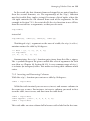
1
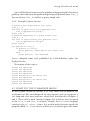
Managing Your Biological
Data with Python
CHAPMAN & HALL/CRC
Mathematical and Computational Biology Series
Aims and scope:
This series aims to capture new developments and summarize what is known
over the entire spectrum of mathematical and computational biology and
medicine. It seeks to encourage the integration of mathematical, statistical,
and computational methods into biology by publishing a broad range of
textbooks, reference works, and handbooks. The titles included in the
series are meant to appeal to students, researchers, and professionals in the
mathematical, statistical and computational sciences, fundamental biology
and bioengineering, as well as interdisciplinary researchers involved in the
field. The inclusion of concrete examples and applications, and programming
techniques and examples, is highly encouraged.
Series Editors
N. F. Britton
Department of Mathematical Sciences
University of Bath
Xihong Lin
Department of Biostatistics
Harvard University
Hershel M. Safer
School of Computer Science
Tel Aviv University
Maria Victoria Schneider
European Bioinformatics Institute
Mona Singh
Department of Computer Science
Princeton University
Anna Tramontano
Department of Physics
University of Rome La Sapienza
Proposals for the series should be submitted to one of the series editors above or directly to:
CRC Press, Taylor & Francis Group
3 Park Square, Milton Park
Abingdon, Oxfordshire OX14 4RN
UK
Published Titles
Algorithms in Bioinformatics: A Practical
Introduction
Wing-Kin Sung
Differential Equations and Mathematical
Biology, Second Edition
D.S. Jones, M.J. Plank, and B.D. Sleeman
Bioinformatics: A Practical Approach
Shui Qing Ye
Dynamics of Biological Systems
Michael Small
Biological Computation
Ehud Lamm and Ron Unger
Engineering Genetic Circuits
Chris J. Myers
Biological Sequence Analysis Using
the SeqAn C++ Library
Andreas Gogol-Döring and Knut Reinert
Exactly Solvable Models of Biological
Invasion
Sergei V. Petrovskii and Bai-Lian Li
Cancer Modelling and Simulation
Luigi Preziosi
Game-Theoretical Models in Biology
Mark Broom and Jan Rychtář
Cancer Systems Biology
Edwin Wang
Gene Expression Studies Using
Affymetrix Microarrays
Hinrich Göhlmann and Willem Talloen
Cell Mechanics: From Single ScaleBased Models to Multiscale Modeling
Arnaud Chauvière, Luigi Preziosi,
and Claude Verdier
Genome Annotation
Jung Soh, Paul M.K. Gordon, and
Christoph W. Sensen
Clustering in Bioinformatics and Drug
Discovery
John D. MacCuish and Norah E. MacCuish
Glycome Informatics: Methods and
Applications
Kiyoko F. Aoki-Kinoshita
Combinatorial Pattern Matching
Algorithms in Computational Biology
Using Perl and R
Gabriel Valiente
Handbook of Hidden Markov Models
in Bioinformatics
Martin Gollery
Computational Biology: A Statistical
Mechanics Perspective
Ralf Blossey
Introduction to Bioinformatics
Anna Tramontano
Introduction to Bio-Ontologies
Peter N. Robinson and Sebastian Bauer
Computational Hydrodynamics of
Capsules and Biological Cells
C. Pozrikidis
Introduction to Computational
Proteomics
Golan Yona
Computational Neuroscience:
A Comprehensive Approach
Jianfeng Feng
Introduction to Proteins: Structure,
Function, and Motion
Amit Kessel and Nir Ben-Tal
Computational Systems Biology of
Cancer
Emmanuel Barillot, Laurence Calzone,
Philippe Hupé, Jean-Philippe Vert, and
Andrei Zinovyev
An Introduction to Systems Biology:
Design Principles of Biological Circuits
Uri Alon
Data Analysis Tools for DNA Microarrays
Sorin Draghici
Kinetic Modelling in Systems Biology
Oleg Demin and Igor Goryanin
Knowledge Discovery in Proteomics
Igor Jurisica and Dennis Wigle
Published Titles (continued)
Managing Your Biological Data with
Python
Allegra Via, Kristian Rother, and
Anna Tramontano
Meta-analysis and Combining
Information in Genetics and Genomics
Rudy Guerra and Darlene R. Goldstein
Methods in Medical Informatics:
Fundamentals of Healthcare
Programming in Perl, Python, and Ruby
Jules J. Berman
Modeling and Simulation of Capsules
and Biological Cells
C. Pozrikidis
Niche Modeling: Predictions from
Statistical Distributions
David Stockwell
Normal Mode Analysis: Theory and
Applications to Biological and Chemical
Systems
Qiang Cui and Ivet Bahar
Optimal Control Applied to Biological
Models
Suzanne Lenhart and John T. Workman
Pattern Discovery in Bioinformatics:
Theory & Algorithms
Laxmi Parida
Python for Bioinformatics
Sebastian Bassi
Quantitative Biology: From Molecular to
Cellular Systems
Sebastian Bassi
Spatial Ecology
Stephen Cantrell, Chris Cosner, and
Shigui Ruan
Spatiotemporal Patterns in Ecology
and Epidemiology: Theory, Models,
and Simulation
Horst Malchow, Sergei V. Petrovskii, and
Ezio Venturino
Statistical Methods for QTL Mapping
Zehua Chen
Statistics and Data Analysis for
Microarrays Using R and Bioconductor,
Second Edition
Sorin Drăghici
Stochastic Modelling for Systems
Biology, Second Edition
Darren J. Wilkinson
Structural Bioinformatics: An Algorithmic
Approach
Forbes J. Burkowski
The Ten Most Wanted Solutions in
Protein Bioinformatics
Anna Tramontano
Managing Your Biological
Data with Python
Allegra Via
Kristian Rother
Anna Tramontano
CRC Press
Taylor & Francis Group
6000 Broken Sound Parkway NW, Suite 300
Boca Raton, FL 33487-2742
© 2014 by Taylor & Francis Group, LLC
CRC Press is an imprint of Taylor & Francis Group, an Informa business
No claim to original U.S. Government works
Version Date: 20130808
International Standard Book Number-13: 978-1-4398-8094-4 (eBook - PDF)
This book contains information obtained from authentic and highly regarded sources. Reasonable efforts
have been made to publish reliable data and information, but the author and publisher cannot assume
responsibility for the validity of all materials or the consequences of their use. The authors and publishers
have attempted to trace the copyright holders of all material reproduced in this publication and apologize to
copyright holders if permission to publish in this form has not been obtained. If any copyright material has
not been acknowledged please write and let us know so we may rectify in any future reprint.
Except as permitted under U.S. Copyright Law, no part of this book may be reprinted, reproduced, transmitted, or utilized in any form by any electronic, mechanical, or other means, now known or hereafter invented,
including photocopying, microfilming, and recording, or in any information storage or retrieval system,
without written permission from the publishers.
For permission to photocopy or use material electronically from this work, please access www.copyright.
com (http://www.copyright.com/) or contact the Copyright Clearance Center, Inc. (CCC), 222 Rosewood
Drive, Danvers, MA 01923, 978-750-8400. CCC is a not-for-profit organization that provides licenses and
registration for a variety of users. For organizations that have been granted a photocopy license by the CCC,
a separate system of payment has been arranged.
Trademark Notice: Product or corporate names may be trademarks or registered trademarks, and are used
only for identification and explanation without intent to infringe.
Visit the Taylor & Francis Web site at
http://www.taylorandfrancis.com
and the CRC Press Web site at
http://www.crcpress.com
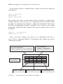
Table of Contents
Preface, xxi
Acknowledgements, xxvii
Part I Getting Started
Chapter 1 ◾ The Python Shell
5
1.1 IN THIS CHAPTER YOU WILL LEARN5
1.2 STORY: CALCULATING THE ΔG OF ATP HYDROLYSIS5
1.2.1 Problem Description
5
1.2.2 Example Python Session
7
1.3 WHAT DO THE COMMANDS MEAN?7
1.3.1 How to Run the Example on Your Computer
8
1.3.2Variables
11
1.3.3 Importing Modules
14
1.3.4Calculations
17
1.4EXAMPLES19
1.5 TESTING YOURSELF21
Chapter 2 ◾ Your First Python Program
23
2.1 IN THIS CHAPTER YOU WILL LEARN23
2.2 STORY: HOW TO CALCULATE THE AMINO ACID
FREQUENCY IN THE SEQUENCE OF INSULIN23
2.2.1 Problem Description
23
2.2.2 Example Python Session
26
vii
viii ◾ Table of Contents
2.3 WHAT DO THE COMMANDS MEAN?26
2.3.1 How to Execute the Program
27
2.3.2 How Does the Program Work?
28
2.3.3Comments
29
2.3.4 String Variables
30
2.3.5 Loops with for33
2.3.6Indentation
34
2.3.7 Printing to the Screen
35
2.4EXAMPLES37
2.5 TESTING YOURSELF38
Part I Summary
Part II Data Management
Chapter 3 ◾ Analyzing a Data Column
45
3.1 IN THIS CHAPTER YOU WILL LEARN45
3.2 STORY: DENDRITIC LENGTHS45
3.2.1 Problem Description
45
3.2.2 Example Python Session
46
3.3 WHAT DO THE COMMANDS MEAN?47
3.3.1 Reading Text Files
47
3.3.2 Writing Text Files
48
3.3.3 Collecting Data in a List
50
3.3.4 Converting Text to Numbers
50
3.3.5 Converting Numbers to Text
51
3.3.6 Writing a Data Column to a Text File
52
3.3.7 Calculations on a List of Numbers
53
3.4EXAMPLES54
3.5 TESTING YOURSELF57
Chapter 4 ◾ Parsing Data Records
59
4.1 IN THIS CHAPTER YOU WILL LEARN59
Table of Contents ◾ ix
4.2 STORY: INTEGRATING MASS SPECTROMETRY DATA
INTO METABOLIC PATHWAYS59
4.2.1 Problem Description
59
4.2.2 Example Python Session
61
4.3 WHAT DO THE COMMANDS MEAN?61
4.3.1The if/elif/else Statements
62
4.3.2 List Data Structures
65
4.3.3 Concise Ways to Create Lists
69
4.4EXAMPLES70
4.5 TESTING YOURSELF75
Chapter 5 ◾ Searching Data
77
5.1 IN THIS CHAPTER YOU WILL LEARN77
5.2 STORY: TRANSLATING AN RNA SEQUENCE INTO
THE CORRESPONDING PROTEIN SEQUENCE77
5.2.1 Problem Description
77
5.2.2 Example Python Session
78
5.3 WHAT DO THE COMMANDS MEAN?80
5.3.1Dictionaries
80
5.3.2The while Statement
82
5.3.3 Searching with while Loops
84
5.3.4 Searching in a Dictionary
84
5.3.5 Searching in a List
85
5.4EXAMPLES86
5.5 TESTING YOURSELF90
Chapter 6 ◾ Filtering Data
93
6.1 IN THIS CHAPTER YOU WILL LEARN93
6.2 STORY: WORKING WITH RNA-SEQ OUTPUT DATA93
6.2.1 Problem Description
93
6.2.2 Example Python Session
96
6.3 WHAT DO THE COMMANDS MEAN?97
6.3.1 Filtering with a Simple for...if Combination
97
x ◾ Table of Contents
6.3.2 Combining Two Data Sets
98
6.3.3 Differences between Two Data Sets
98
6.3.4 Removing from Lists, Dictionaries, and Files
99
6.3.5 Removing Duplicates Preserving and Not
Preserving Order
102
6.3.6Sets
104
6.4EXAMPLES106
6.5 TESTING YOURSELF108
Chapter 7 ◾ Managing Tabular Data
111
7.1 IN THIS CHAPTER YOU WILL LEARN111
7.2 STORY: DETERMINING PROTEIN CONCENTRATIONS111
7.2.1 Problem Description
111
7.2.2 Example Python Session
113
7.3 WHAT DO THE COMMANDS MEAN?114
7.3.1 Representing a Two-Dimensional Table
114
7.3.2 Accessing Rows and Single Cells
115
7.3.3 Inserting and Removing Rows
116
7.3.4 Accessing Columns
117
7.3.5 Inserting and Removing Columns
119
7.4EXAMPLES121
7.5 TESTING YOURSELF127
Chapter 8 ◾ Sorting Data
129
8.1 IN THIS CHAPTER YOU WILL LEARN129
8.2 STORY: SORT A DATA TABLE129
8.2.1 Problem Description
129
8.2.2 Example Python Session
130
8.3 WHAT DO THE COMMANDS MEAN?130
8.3.1 Python Lists Are Good for Sorting
130
8.3.2The sorted() Built-in Function
133
8.3.3 Sorting with itemgetter133
8.3.4 Sorting in Ascending/Descending Order
134
Table of Contents ◾ xi
8.3.5 Sorting Data Structures (Tuples, Dictionaries)
135
8.3.6 Sorting Strings by Their Length
137
8.4EXAMPLES137
8.5 TESTING YOURSELF141
Chapter 9 ◾ Pattern Matching and Text Mining
143
9.1 IN THIS CHAPTER YOU WILL LEARN143
9.2 STORY: SEARCH A PHOSPHORYLATION MOTIF IN A
PROTEIN SEQUENCE143
9.2.1 Problem Description
143
9.2.2 Example Python Session
145
9.3 WHAT DO THE COMMANDS MEAN?145
9.3.1 Compiling Regular Expressions
145
9.3.2 Pattern Matching
146
9.3.3 Grouping148
9.3.4 Modifying Strings
150
9.4EXAMPLES154
9.5 TESTING YOURSELF158
Part II Summary
Part III Modular Programming
Chapter 10 ◾ Divide a Program into Functions
167
10.1 IN THIS CHAPTER YOU WILL LEARN167
10.2 STORY: WORKING WITH THREE-DIMENSIONAL
COORDINATE FILES167
10.2.1 Problem Description
167
10.2.2 Example Python Session
169
10.3 WHAT DO THE COMMANDS MEAN?170
10.3.1 How to Define and Call Functions
172
10.3.2 Function Arguments
175
10.3.3The struct Module
179
xii ◾ Table of Contents
10.4EXAMPLES181
10.5 TESTING YOURSELF185
Chapter 11 ◾ Managing Complexity with Classes
189
11.1 IN THIS CHAPTER YOU WILL LEARN189
11.2 STORY: MENDELIAN INHERITANCE189
11.2.1 Problem Description
189
11.2.2 Example Python Session
190
11.3 WHAT DO THE COMMANDS MEAN?191
11.3.1 Classes Are Used to Create Instances
192
11.3.2 Classes Contain Data in the Form of Attributes
194
11.3.3 Classes Contain Methods
195
11.3.4The _ _repr__ Method Makes Classes
and Instances Printable
196
11.3.5 Using Classes Helps to Master
Complex Programs197
11.4EXAMPLES199
11.5 TESTING YOURSELF201
Chapter 12 ◾ Debugging205
12.1 IN THIS CHAPTER YOU WILL LEARN205
12.2 STORY: WHEN YOUR PROGRAM DOES NOT WORK205
12.2.1 Problem Description
205
12.2.2 Example Python Session
207
12.3 WHAT DO THE COMMANDS MEAN?208
12.3.1 Syntax Errors
208
12.3.2 Runtime Errors
210
12.3.3 Handling Exceptions
213
12.3.4 When There Is No Error Message
215
12.4EXAMPLES219
12.5 TESTING YOURSELF222
Table of Contents ◾ xiii
Chapter 13 ◾ Using External Modules: The Python
Interface to R
225
13.1 IN THIS CHAPTER YOU WILL LEARN225
13.2 STORY: READING NUMBERS FROM A FILE AND
CALCULATING THEIR MEAN VALUE USING R WITH
PYTHON225
13.2.1 Problem Description
225
13.2.2 Example Python Session
227
13.3 WHAT DO THE COMMANDS MEAN?228
13.3.1The robjects Object of rpy2 and the r
Instance228
13.3.2 Accessing an R Object from Python
228
13.3.3 Creating Vectors
230
13.3.4 Creating Matrices
231
13.3.5 Converting Python Objects into R Objects
234
13.3.6 How to Deal with Function Arguments That
Contain a Dot
235
13.4EXAMPLES236
13.5 TESTING YOURSELF241
Chapter 14 ◾ Building Program Pipelines
245
14.1 IN THIS CHAPTER YOU WILL LEARN245
14.2 STORY: BUILDING AN NGS PIPELINE245
14.2.1 Problem Description
245
14.2.2 Example Python Session
247
14.3 WHAT DO THE COMMANDS MEAN?247
14.3.1 How to Use TopHat and Cufflinks
249
14.3.2 What Is a Pipeline?
249
14.3.3 Exchanging Filenames and Data between Programs 251
14.3.4 Writing a Program Wrapper
252
14.3.5 Lag When Closing Files
253
14.3.6 Using Command-Line Parameters
254
xiv ◾ Table of Contents
14.3.7 Testing Modules: if __name__ == ' __
main__ '255
14.3.8 Working with Files and Directories
256
14.4EXAMPLES258
14.5 TESTING YOURSELF260
Chapter 15 ◾ Writing Good Programs
263
15.1 IN THIS CHAPTER YOU WILL LEARN263
15.2 PROBLEM DESCRIPTION: UNCERTAINTY263
15.2.1 There Is Uncertainty in Writing Programs
263
15.2.2 Example Programming Project
264
15.3 SOFTWARE ENGINEERING265
15.3.1 Dividing a Programming Project into Smaller Tasks 265
15.3.2 Split a Program into Functions and Classes
267
15.3.3 Writing Well-Formatted Code
270
15.3.4 Using a Repository to Control Program Versions
271
15.3.5 How to Release Your Program to Other People
273
15.3.6 The Cycle of Software Development
275
15.4EXAMPLE278
15.5 TESTING YOURSELF280
Part III Summary
Part IV Data Visualization
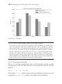
Chapter 16 ◾ Creating Scientific Diagrams
287
16.1 IN THIS CHAPTER YOU WILL LEARN287
16.2 STORY: NUCLEOTIDE FREQUENCIES IN THE
RIBOSOME287
16.2.1 Problem Description
288
16.2.2 Example Python Session
288
16.3 WHAT DO THE COMMANDS MEAN?289
16.3.1The matplotlib Library
289
Table of Contents ◾ xv
16.3.2 Drawing Vertical Bars
290
16.3.3 Adding Labels to an x-Axis and y-Axis291
16.3.4 Adding Tick Marks
291
16.3.5 Adding a Legend Box
292
16.3.6 Adding a Figure Title
292
16.3.7 Setting the Boundaries of the Diagram
292
16.3.8 Exporting an Image File in Low Resolution and
High Resolution
292
16.4EXAMPLES293
16.5 TESTING YOURSELF298
Chapter 17 ◾ Creating Molecule Images with PyMOL
301
17.1 IN THIS CHAPTER YOU WILL LEARN301
17.2 STORY: THE ZINC FINGER301
17.2.1 What Is PyMOL?
302
17.2.2 Example PyMOL Session
305
17.3 SEVEN STEPS TO CREATE A HIGH-RESOLUTION
IMAGE306
17.3.1 Writing PyMOL Script Files
307
17.3.2 Loading and Saving Molecules
307
17.3.3 Selecting Parts of Molecules
309
17.3.4 Choose Representations for Each Selection
313
17.3.5 Setting Colors
315
17.3.6 Setting the Camera Position
316
17.3.7 Exporting a High-Resolution Image
317
17.4EXAMPLES319
17.5 TESTING YOURSELF321
Chapter 18 ◾ Manipulating Images
323
18.1 IN THIS CHAPTER YOU WILL LEARN323
18.2 STORY: PLOT A PLASMID323
18.2.1 Problem Description
324
18.2.2 Example Python Session
325
xvi ◾ Table of Contents
18.3 WHAT DO THE COMMANDS MEAN?326
18.3.1 Creating an Image
327
18.3.2 Reading and Writing Images
327
18.3.3Coordinates
328
18.3.4 Drawing Geometrical Shapes
329
18.3.5 Rotating an Image
331
18.3.6 Adding Text Labels
331
18.3.7Colors
332
18.3.8 Helper Variables
333
18.4EXAMPLES334
18.5 TESTING YOURSELF336
Part IV Summary
Part V Biopython
Chapter 19 ◾ Working with Sequence Data
347
19.1 IN THIS CHAPTER YOU WILL LEARN347
19.2 STORY: HOW TO TRANSLATE A DNA CODING
SEQUENCE INTO THE CORRESPONDING PROTEIN
SEQUENCE AND WRITE IT TO A FASTA FILE347
19.2.1 Problem Description
347
19.2.2 Example Python Session
348
19.3 WHAT DO THE COMMANDS MEAN?348
19.3.1The Seq Object
349
19.3.2 Working with Sequences as Strings
352
19.3.3The MutableSeq Object
353
19.3.4The SeqRecord Object
354
19.3.5The SeqIO Module
356
19.4EXAMPLES358
19.5 TESTING YOURSELF361
Table of Contents ◾ xvii
Chapter 20 ◾ Retrieving Data from Web Resources
363
20.1 IN THIS CHAPTER YOU WILL LEARN363
20.2 STORY: SEARCHING PUBLICATIONS BY
KEYWORDS IN PUBMED AND DOWNLOADING
AND PARSING THE CORRESPONDING RECORDS363
20.2.1 Problem Description
363
20.2.2 Python Session
364
20.3 WHAT DO THE COMMANDS MEAN?365
20.3.1The Entrez Module
365
20.3.2The Medline Module
367
20.4EXAMPLES368
20.5 TESTING YOURSELF372
Chapter 21 ◾ Working with 3D Structure Data
375
21.1 IN THIS CHAPTER YOU WILL LEARN375
21.2 STORY: EXTRACTING ATOM NAMES AND THREEDIMENSIONAL COORDINATES FROM A PDB FILE375
21.2.1 Problem Description
376
21.2.2 Example Python Session
376
21.3 WHAT DO THE COMMANDS MEAN?376
21.3.1The Bio.PDB Module
376
21.3.2 The SMCRA Object Hierarchy
378
21.4EXAMPLES384
21.5 TESTING YOURSELF388
Part V Summary
Part VI Cookbook
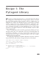
RECIPE 1: THE PYCOGENT LIBRARY, 395
RECIPE 2: REVERSING AND RANDOMIZING A SEQUENCE, 399
xviii ◾ Table of Contents
RECIPE 3: CREATING A RANDOM SEQUENCE WITH
PROBABILITIES, 403
RECIPE 4: PARSING MULTIPLE SEQUENCE ALIGNMENTS
USING BIOPYTHON, 405
RECIPE 5: C
ALCULATING A CONSENSUS SEQUENCE FROM A
MULTIPLE SEQUENCE ALIGNMENT, 409
RECIPE 6: CALCULATING THE DISTANCE BETWEEN
PHYLOGENETIC TREE NODES, 413
RECIPE 7: CODON FREQUENCIES IN A NUCLEOTIDE
SEQUENCE, 417
RECIPE 8: PARSING RNA 2D STRUCTURES IN THE VIENNA
FORMAT, 421
RECIPE 9: PARSING BLAST XML OUTPUT, 425
RECIPE 10: PARSING SBML FILES, 427
RECIPE 11: RUNNING BLAST, 431
RECIPE 12: ACCESSING, DOWNLOADING, AND READING
WEB PAGES, 437
RECIPE 13: PARSING HTML FILES, 441
RECIPE 14: SPLITTING A PDB FILE INTO PDB CHAIN FILES, 445
RECIPE 15: FINDING THE TWO CLOSEST CΑ ATOMS IN A
PDB STRUCTURE, 447
RECIPE 16: EXTRACTING THE INTERFACE BETWEEN TWO
PDB CHAINS, 451
Table of Contents ◾ xix
RECIPE 17: BUILDING HOMOLOGY MODELS USING
MODELLER, 455
RECIPE 18: RNA 3D HOMOLOGY MODELING WITH
MODERNA, 459
RECIPE 19: CALCULATING RNA BASE PAIRS FROM A 3D
STRUCTURE, 463
RECIPE 20: A REAL CASE OF STRUCTURAL
SUPERIMPOSITION: THE SERINE PROTEASE
CATALYTIC TRIAD, 467
APPENDIX A: COMMAND OVERVIEW, 471
APPENDIX B: PYTHON RESOURCES, 495
APPENDIX C: RECORD SAMPLES, 499
APPENDIX D: HANDLING DIRECTORIES
AND PROGRAMS WITH UNIX, 507
Preface
Only a few years ago, programming was a prerogative of computational
scientists. Notwithstanding this, programming is increasingly becoming
a need of specialists in other fields such as biology. As a biologist, you are
not necessarily interested in becoming an expert programmer, but you
want to continue your scientific endeavors using programming as one of
many tools. You may already have realized that programming techniques
would dramatically speed up the management and analysis of your data.
Maybe you want to deal with large amounts of data, repeat the same kind
of analysis several times, or parse files with unusual formats. We can assure
you that in all these cases programming is very useful. However, you may
feel uncomfortable because you never had much interest in a “dry” and
“conceptually hard” discipline such as computer science. In that case, this
book is for you.
We wrote this book for life scientists who want to have more control
of their data and, for this, need to learn some programming. It is aimed
at empowering biologists without prior programming experience to work
with biological data on their own using Python.
In the Preface, you will find a summary of what you can learn reading
this book and an introduction of what a program is, followed by an overview of the Python programming language.
We hope that this book on programming is tailored to your needs as a
biologist and will help you analyze your data and thus increase the likelihood to make better discoveries.
WHAT YOU CAN LEARN FROM THIS BOOK
In this book you will learn not only how to program but also how to
manage your data, which means reading data from files, analyzing and
manipulating them, and writing the results to a file or to the computer
screen. Every single piece of code described in the book is aimed at solving
xxi
xxii ◾ Preface
biological problems; every example deals with biological questions. The
book proposes as many different cases as possible; covers many strategies to organize, analyze, and present data; and solves biological problems
in the form of “programming recipes.” Exercises that you can use to test
yourself or include in a programming course for biologists appear at the
end of each chapter.
The book is organized in six parts and contains twenty-one chapters
in total. Part I introduces the Python language and teaches you how to
write your first programs. Part II introduces all the basic elements of the
language, enabling you to write small programs independently. Part III is
about creating bigger programs using techniques to write well-organized,
efficient, and error-free code. Part IV is devoted to data visualization. You
will learn how to plot your data, or draw a figure for an article or a slide
presentation. It also introduces PyMOL, a program to visualize macromolecular structures. Part V introduces you to Biopython, a programming
library that helps with reading and writing several biological file formats
and facilitates querying the NCBI databases online and retrieving biological records from the web. Part VI is a cookbook containing twenty specific
programming “recipes,” ranging from secondary structure prediction and
multiple sequence alignment analyses to superimposing protein threedimensional structures.
Furthermore, the book has four appendices. Appendix A provides an
overview of both Python and UNIX commands. Appendix B lists several
links to Python resources freely available on the web. Appendix C contains sample file formats cited throughout the book, such as a sequence
in FASTA format, a sequence in GenBank format, a PDB file, an MSA
example, etc. Finally, Appendix D is a short UNIX tutorial.
WHAT IS PROGRAMMING?
This book will teach you how to write programs. What exactly is a program? A program is conceptually similar to a cooking recipe. Like a recipe
lists ingredients and kitchenware at the beginning, a program needs to
define what objects (data and functions) are necessary. For instance, you
could define a given DNA sequence as your data and define a function that
calculates the GC-content in it. A recipe also contains a list of actions that
must be carried out to use ingredients and kitchenware to prepare a dish.
Likewise, a program contains a written list of elementary instructions
such as “read the DNA sequence from a file,” “calculate the GC-content,”
Preface ◾ xxiii
or “print the GC-content to the screen.” Creating a program means writing instructions in a suitable language (e.g., Python), typically to a text
file. Running a program means executing the instructions (i.e., the lines of
code) listed in the program.
There is one big difference between kitchen recipes and computer programs, though: a human cook can divert from the recipe and add ingredients creatively or react to unexpected mishaps, which is important to
obtain a tasty meal! A computer, however, is never creative. It reads the
instructions in the program one by one and executes them by the letter.
On one hand, the lack of computer creativity makes it necessary for you
to explicitly tell it every tiny step, which can sometimes be unnerving.
Imagine you are talking to a cook who is intellectually disabled but incredibly fast. On the other hand, computer predictability makes it easy to precisely repeat instructions many times. Imagine what a cook would say to
an order of 100,000 identical dishes! Programming means using the rigid
logics of computers to your advantage.
You must be aware that most of programming happens in your head.
When you struggle to write a program, it may be helpful to formulate
small step-by-step instructions in human language first. When the overall structure of your program is ready and you know exactly what you
want it to do, it is time to start writing instructions. To do this, you need a
programming language. In fact, programming basically consists of writing instructions in a given language to a text file or to a special terminal
shell and telling your computer to execute them. The lines containing
instructions are commonly called source code. Accordingly, programming or coding means writing source code. Since computers do not
understand English, Italian, or German, you need to use a programming
language to write source code. Our favorite language for answering biological questions is Python.
WHY PYTHON?
Python is simple to learn. It is a high-level programming language that
is interpreted and object oriented. Let’s analyze these concepts one by
one.
Python Is Simple to Learn
A program can be written in one of many programming languages: C,
C++, Fortran, Perl, Java, Pascal, etc. Every programming language has
xxiv ◾ Preface
formal rules and keywords (the syntax) and semantics (meaning). A key
advantage of Python is that code is easy to read. Code can be more or less
comprehensible to humans; for example, the Python instruction
print 'ACGT'
is quite intuitive (the computer will print the text ACGT to the screen),
whereas the Perl instruction
$cmd = "imgcvt -i $intype -o $outtype $old.$num";
is less intuitive. Python is, compared to other programming languages,
relatively similar to English and has a very simple syntax. We think this
makes Python easy to learn for biologists.
Python Is a High-Level Programming Language
Python can also be used to do very complex things. You can represent
complex data types like trees and networks, start other programs (e.g.,
bioinformatics applications) from Python, and download web pages. You
also have tools to detect and handle errors in your programs. Finally,
Python is not optimized for any particular purpose; it is therefore well
apt to glue together other programs, web services, and databases in order
to build customized scientific pipelines with a few lines of source code.
Python Is Interpreted
Some programming languages are interpreted, and some are compiled.
For computers to execute a program, they need to translate the instructions to binary machine code, which is unreadable even for experienced
programmers. In an interpreted language, each line is translated and executed one after another. In a compiled language, first the whole program
is translated and only then executed. Execution of compiled languages is
generally much faster than execution of interpreted ones. However, you
need to compile the program each time you change something. With an
interpreted language, you can see the effect of your changes immediately
and, as a result, write programs faster. Therefore, we think that an interpreted language like Python is much easier to start with.
Python Is Object Oriented
In Python, everything is an object. Objects are independent program components representing data and instructions. They allow you to connect
Preface ◾ xxv
data with useful functionalities (e.g., you could have a sequence object that
contains a DNA sequence and functions for transcribing and translating
this sequence). Objects help to structure complex programs and make
program components reusable.
Using Python, many developers have made reusable objects available
in programming libraries. For instance, reading and parsing a FASTA
sequence file using Biopython can be done in two lines of code. Without
the library, you would have to write ten to thirty lines, depending on the
programming language. Therefore, object orientation in Python helps you
to write short programs.
In conclusion, we believe that Python is an ideal language for those who
want to have fun with little or no pain and learn programming to pragmatically manage biological data, solve biological problems, and widen
the horizon of their scientific discoveries. We hope you will enjoy using
this book at least as much as we enjoyed writing it!
Code Downloads
All code examples presented in this book are available online at https://
bitbucket.org/krother/python-for-biologists, following the “Source” link.
Acknowledgements
We would like to thank the students and trainees to whom we had the
privilege to teach Python. Your questions, problems, and ideas during
Python courses over the past seven years are the main source of inspiration for this book. We can’t name all of you, but we want you to know
that we learned much from your enthusiasm, cheerfulness, frustration,
and success.
Special thanks go to Pedro Fernandes, a great course organizer, who
provided us with the opportunity to condense existing material into a
five-day course at the Gulbenkian Institute in Portugal. We learned many
of the key questions of this book during these courses and during afterdinner discussions in Astrolabio.
Additional credit goes to Janusz M. Bujnicki, Artur Jarmolowski, Jakub
Nowak, Edward Jenkins, Amelie Anglade, Janick Mathys, and Victoria
Schneider for providing various Python training opportunities.
We are also grateful to Francesco Cicconardi for his help with the
RNA-Seq output parser and the NGS pipeline on which Chapters 6 and
14 are respectively based. He not only suggested us a typical NGS pipeline
but also provided code and verified that the biological and computational
discussions of the problem were correct and exhaustive.
We would like to thank Justyna Wojtczak, Katarzyna Potrzebowska,
Wojciech Potrzebowski, Kaja Milanowska, Tomasz Puton, Joanna Kasprzak,
Anna Philips, Teresa Szczepinska, Peter Cock, Bartosz Telenczuk, Patrick
Yannul, Gavin Huttley, Rob Knight, Barbara Uszczynska, Fabrizio Ferre’,
Markus Rother, and Magdalena Rother for providing examples and constructive feedback.
Finally, many thanks to Alba Lepore for discussions during the realization of the book and for key help in accomplishing the book’s cover.
xxvii
I
Getting Started
INTRODUCTION
For the four brave Python apprentices who made it to the mountaintop
during the Python and Friends Conference 2010 in Karpacz, Poland.
When you want to climb high mountains, what do you do? If you are
good at mountain climbing, you gather your equipment, call up some
fellow climbers, pick a mountain, and move out. In the stories written by
professional mountain climbers, you will find that they use ropes, hooks,
oxygen bottles, and sometimes nothing more than their bare hands. They
fight with icy storms at altitudes of 4,000 meters and above, coordinate big
teams distributed over several camps, and survive in the deadly zone near
the mountaintop.
But what if you are a beginner interested in mountain climbing? Do
you strap on the oxygen bottles and move out? No. Instead, you will probably start with an easy mountain. There are mountains with safe, clearly
marked paths to the top. All you need is a map and a pair of boots. Still, the
sight from the top of such a mountain can be breathtaking.
Programming is very similar to that. As a biologist learning to program, you do not need fancy equipment or tons of theoretical knowledge.
Even simple programs can be powerful tools to master your data. A lot of
programming can be done by collecting working fragments of code and
1
2 ◾ Managing Your Biological Data with Python
then assembling and modifying them. The result may not be as elegant
as a program written by a computer scientist, but it may solve a problem
quickly. Your problem.
We want this book to be the map that helps you to climb the mountains of
everyday data management. We want programming to make your life easier
without you necessarily becoming a professional software developer first.
In the first part, we would like you to make your first steps in the
Python programming language. You will see that commands in Python
are very intuitive and close to the English language, so you won’t need
much effort to learn and remember most of the Python instructions. For
example, if you want to calculate the length of a sequence, you just have to
type len('MALWMRLLPLLALLALWGPDPAA…'). The aim of the two chapters of Part I is not only to show how simple the Python syntax is but also
to make you scent the clever structure of the language. Python basically
consists of a set of modules (typically files where programming instructions are written) that you can connect to each other.
When learning a new language, e.g., German, you may start by reading a text and analyzing the nature, role, and position in the text of each
word. After reading and analyzing many texts, you will be able to extract
language rules and write your own texts. Alternatively, you can first learn
what kinds of object categories make up the language nouns, verbs, adjectives, etc. and the links between them (e.g., prepositions or German cases)
and then use the structure of the language, associated with a good dictionary, to write your texts. In this part of the book, you will start grasping that
Python is basically another language like English or German. In fact, it is
made up of a limited number of object types (nouns, verbs, etc.) that you
can connect to each other to form sentences. In this book, we blend the
two approaches described previously to learn German, by alternating code
examples that you can analyze and try with the explanation of language
object categories. To indicate what specific objects belong to each category,
Python provides a very good online dictionary, which is called the Python
Standard Library (http://docs.python.org/2/library/), where you can look
up the meaning of single words. Once the structure of the language is clear
to you, and you are able to play with the various object categories, most
will be done: at that stage you can basically improve your knowledge of the
language by increasing your vocabulary or using the dictionary efficiently.
The last step of learning is related to the good design of programs. This is
in general good practice and may turn out to be very useful if you need
to write big programs, efficiently collaborate with other programmers,
Getting Started ◾ 3
maintain or extend your or other people’s programs in the future, increase
the performance of your work, or want to become an expert programmer,
but it is not really indispensable in order to accomplish the tasks presented
in this book. In any case, we will provide plenty of suggestions on how to
write good programs in the second part of the book.
In Chapter 1, you will learn how to use the Python shell where you can
enter simple commands. The simplest operations are similar to those on a
pocket calculator. For instance, if you use the Python shell, you will see a
prompt that looks like this: >>>. If you enter a simple mathematical operation at the right of the prompt and press the Enter key,
>>> 1 + 1
you get the result 2 immediately. You will also encounter variables as
a way to store your data. You will learn how to perform calculations
with numbers and to import and use a mathematical module that gives
you extra functions like square roots and logarithms. In Chapter 2, you
will write your first Python program. The program will be for counting
amino acids in a protein sequence. For that you will need strings, a data
structure for storing text. You will use a control flow structure for repeating instructions automatically, instead of writing the same line over and
over. At the end of Part I, you will know most of the basic parts of the
Python language.
Chapter
1
The Python Shell
L
earning goal: You can use Python as a scientific calculator.
1.1 IN THIS CHAPTER YOU WILL LEARN
• How to use the Python shell as a scientific calculator
• How to calculate the ΔG of ATP hydrolysis
• How to calculate the distance between two points
• How to create your own Python module
1.2 STORY: CALCULATING THE ΔG OF ATP HYDROLYSIS
1.2.1 Problem Description
ATP → ADP + Pi
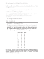
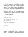
The hydrolysis of one phosphodiester bond from ATP results in a standard
Gibbs energy (ΔG0) of –30.5 kJ/mol. According to biochemistry textbooks,
the real ΔG value depends on the concentration of the compounds. And
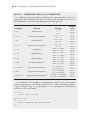
these concentrations can differ quite a lot among tissues (see Table 1.1,
according to Berg et al.*).
*
Jeremy M. Berg, John L. Tymoczko, and Lubert Stryer, Biochemistry, 5th ed. (New York: W. H.
Freeman, 2002).
5
6 ◾ Managing Your Biological Data with Python
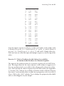
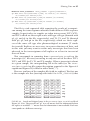
TABLE 1.1 Compound Concentration in Different Tissues.
Tissue
Liver
Muscle
Brain
[ATP] [mM]
3.5
8.0
2.6
[ADP] [mM]
1.8
0.9
0.7
[Pi][mM]
5.0
8.0
2.7
How can the real ΔG value for ATP hydrolysis be calculated? The Gibbs
energy as a function of the concentrations of the compounds can be written as
ΔG = ΔG0 + RT * ln ([ADP] * [Pi] / [ATP])
You can insert values from the table into this equation with many tools
(e.g., a pocket calculator, the Windows calculator application, or your
mobile phone). In this book, you are going to learn a much more efficient
and powerful tool for calculations and data management: the Python programming language.
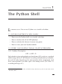
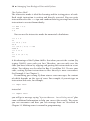
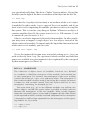
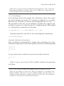
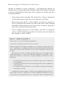
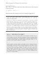
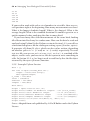
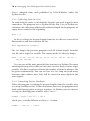
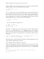
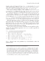
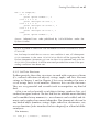
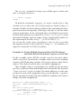
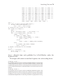
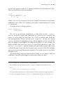
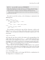
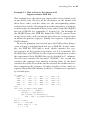
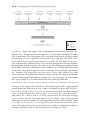
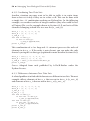
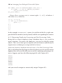
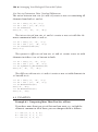
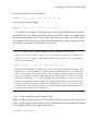
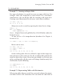
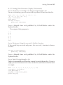
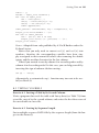
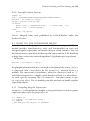
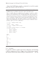
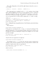
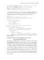
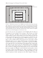
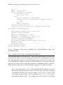
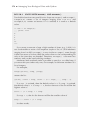
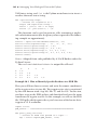
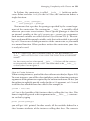
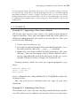
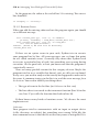
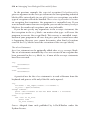
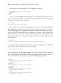
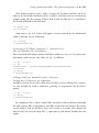
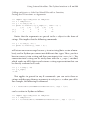
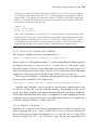
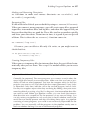
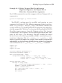
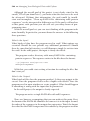
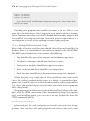
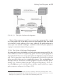
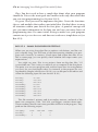
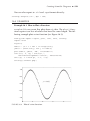
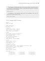
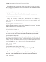
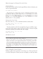
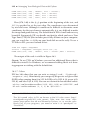
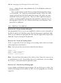
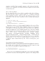
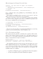
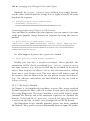
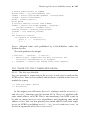
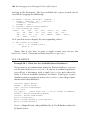
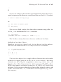
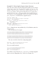
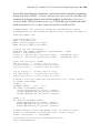
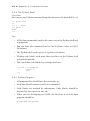
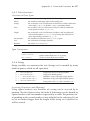
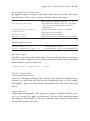
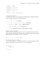
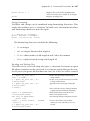
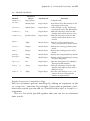
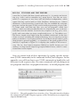
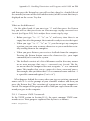
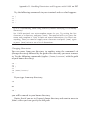
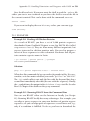
Using Python, you can do the calculation for liver tissue in the interactive Python interpreter (see Figure 1.1). The prompt >>> indicates the
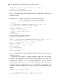
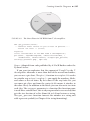
FIGURE 1.1 The Python shell. Note: To start it you have to type “python” at
the prompt of the UNIX terminal shell (in UNIX/Linux or Mac OS X) or start
‘Python (command line)’ from the program menu (in Windows).
The Python Shell ◾ 7 place where you can enter commands, and it appears when you start a
Python interactive session (see Section 1.3.1). Python commands must be
typed just at the right side of the prompt.
1.2.2 Example Python Session
>>> ATP = 3.5
>>> ADP = 1.8
>>> Pi = 5.0
>>> R = 0.00831
>>> T = 298
>>> deltaG0 = -30.5
>>>
>>> import math
>>> deltaG0 + R * T * math.log(ADP * Pi / ATP)
-28.161154161098693
Source: Adapted from code published by A.Via/K.Rother under the
Python License.
1.3 WHAT DO THE COMMANDS MEAN?
In programming, most of what you do can be roughly summarized in
five points: organize data, use other programs, calculate things, and
read and write data. The previous example contains three. First, it organizes the parameters for the ΔG formula by storing them in variables.
Variables are containers that help you not to write the same numbers
repeatedly. Second, it uses an external program to calculate the logarithm: the math.log(x) function calculates the logarithm of x and is
accessed through the import statement, which makes available extra
Python functions by connecting a program to other modules (math in
the example) where such functions are stored. Modules are programming units collecting variables, functions, and other useful objects. They
are always stored in files. See Box 1.1 for more on the import statement
and Python modules.
Finally, the example in Section 1.2.2 calculates the ΔG value. Simple
arithmetical calculations work very similar to a pocket calculator. The second part of this book is dedicated to other ways in which you can manipulate your data. The first thing you can try to do yourself is to start the
calculation in the previous section.
8 ◾ Managing Your Biological Data with Python
BOX 1.1 THE import STATEMENT AND THE
CONCEPT OF MODULES
When you write
>>> import math
you are connecting to the math module. What exactly is math? math is
a file on your computer; its actual name is math.py. The .py extension
stands for Python, and the file contains Python instructions, i.e., definitions of variables and functions and instructions (for calculating things).
The math.py file, in particular, contains instructions for the definition and
calculation of mathematical functions (e.g., sqrt(), log(), etc.).
In Python, text files that contain Python instructions are called modules.
The import instruction is needed to access an external module and read its
content. This way, all the definitions present in a module will become available when you import it: effectively, the code is shared and can be used in
many different programs.
How can you know which mathematical functions are defined in the
math module? Either you can browse the Internet and find and open the
file math.py and read its contents, or you can use the instruction
>>> import math
>>> dir(math)
You can use the dir(math) instruction only after having imported the math
module, otherwise the dir() function does not know what its argument is.
As a result, you will see a complete list of variables and functions present in
the math module:
['__doc__', '__name__', '__package__', 'acos', 'acosh',
'asin', 'asinh', 'atan', 'atan2', 'atanh', 'ceil', 'copysign', 'cos', 'cosh', 'degrees', 'e', 'exp', 'fabs',
'factorial', 'floor', 'fmod', 'frexp', 'fsum', 'hypot',
'isinf', 'isnan', 'ldexp', 'log', 'log10', 'log1p',
'modf', 'pi', 'pow', 'radians', 'sin', 'sinh', 'sqrt',
'tan', 'tanh', 'trunc']
You can get a short explanation of each function by typing, for instance,
>>> help(math.sqrt)
1.3.1 How to Run the Example on Your Computer
The Python programming language is a program that needs to be started
before you can use it. On Linux (Ubuntu) and Mac OS X, Python is already
The Python Shell ◾ 9 installed and can be started from a text console by typing “python” at the
command line prompt. See Appendix D to learn how to run a program
from a text terminal. On Windows, you need to install Python first and
then start a Python shell window in ‘Start’ → ‘All programs’ → ‘Python’
→ ‘IDLE or Python (command line)’. First, download Python 2.7 from
www.python.org. Install it, then start ‘Python (command line)’ from the
program menu. For more details, see Box 1.2. When you see the >>> sign
in a text window on your screen, you have succeeded and are ready to
write program code (see Figure 1.1). The Python shell can be exited by
typing Ctrl+D.
BOX 1.2 HOW TO INSTALL PYTHON
On Linux and Mac OS X, Python is already installed. In rare cases where
it is not, you can get the most recent version from the package manager or
by typing at a command terminal:
sudo apt-get install python
On Windows you need to download the Python Windows installer
from www.python.org. Make sure you download version 2.7 of Python.
Versions 3.0 and above are at the time of writing experimental and not
compatible with this book. The programming language can be installed like
most programs by clicking and accepting the defaults.
To check whether your installation was successful, you should start
Python. There are two ways to run Python code:
1.Using the interactive mode (Python shell). On Linux and Mac OS X,
you type “python” from a text console and press Enter. On Windows
you choose ‘Start’ → ‘Programs’ → ‘Python 2.7’ → ‘Python (command line)’. The Python shell will start in a separate window.
Alternatively, you can open a text console by entering “cmd” in the
‘Start’ → ‘Execute’ dialog, then change the directory to C:\Python27
and type “python” there. When you see the prompt >>>, your installation is successful.
2.Writing code into a script file having the .py extension (e.g., my_
script.py) and executing the script by typing at the UNIX/Linux
shell prompt:
python my_script.py
See also Section 2.3.1, “How to Execute the Program.”
10 ◾ Managing Your Biological Data with Python
The Python Shell
The interactive mode is ideal for learning and for testing pieces of code.
Each single instruction is written and directly executed. You can write
instructions after the >>> sign and confirm them by pressing Enter. Each
instruction is executed immediately.
>>> ATP = 3.5
>>> ATP
3.5
You can use the interactive mode for numerical calculations:
>>> 3 * 4
12
>>> 12.5 / 0.5
25.0
>>> (12.5 / 0.5) * 100
2500.0
>>> 3 ** 4
81
>>> 3 ** (4 + 2)
729
A disadvantage of the Python shell is that when you exit the session (by
typing Ctrl+D), your code gets lost. Therefore, you can only save the
code you have written by copying and pasting the instructions to a text
editor. Text editors are described in Box 2.2 and Box D.2. To save your
code, writing Python instructions to files directly is more convenient.
See Example 1.1 or Chapter 2.
If something goes wrong, Python returns error messages, the content
of which depends on the type of error. For example, if you mistype an
instruction and write, for example,
>>> imprt math
instead of
>>> import math
you will get a message saying “SyntaxError: invalid syntax” plus
some additional information to help you correct the error(s). The errors
you can encounter and how you can manage them are described in
Chapter 12. Making errors is normal in programming.
The Python Shell ◾ 11 1.3.2 Variables
In Section 1.2.2, a number of variables are initially defined. That is, the
values to be used in the calculation are put into named containers.
For example, when writing
>>> ATP = 3.5
the computer will remember the number 3.5 under the name ATP, so
when you write later
>>> ATP
the computer will print the value 3.5.
In the same way, all numbers used (1.8, 5.0, 0.00831, 298, and –30.5)
are recorded each in its own variable (ADP, Pi, R, T, and deltaG0, respectively). Note that none of the numbers have a unit. Like when using a
pocket calculator, you need to take care to convert them properly. This is
why for the gas constant R (8.31 J/kmol) the value
>>> R = 0.00831
is used, so that it fits to the unit of ΔG 0 (kJ/kmol). As with a pocket
calculator, you are responsible for converting numbers to appropriate
units.
Each kind of object can be stored in a variable. In other words, you can
“label” a piece of data with a name and, instead of writing the whole data
every time you need it, you can just use the name of the variable. The more
complex and the more frequently used the data are (e.g., the nucleotide
sequence of a whole gene), the more convenient it is to use a variable name
in its place.
So, if you want to use the Gibbs energy value for ATP hydrolysis
ΔG0 = –30.5 kJ/mol
several times, it would be better to put it into a variable and use the variable name instead of the whole number.
The operator used to assign an object to a variable name is the equal
sign =:
>>> deltag = –30.5
12 ◾ Managing Your Biological Data with Python
Python distinguishes between integer and floating-point numbers:
>>> a = 3
>>> b = 3.0
In Python jargon, we say that the two variables a and b have different
data types. The variable a is an integer; b is a float. Their difference can be
seen when you divide these numbers by another integer:
>>> a / 2
1
>>> b / 2
1.5
You can enforce conversion of an integer to a float number by dividing
the integer by a float:
>>> a / 2.0
1.5
You can assign numbers, text, and many other kinds of data to variables. More generally, you can refer to the data as Python objects. In
the following example, you assign a floating-point number object to a
variable:
>>> deltag = –30.5
If you assign a new value to an existing variable name, the second value
will overwrite the first. In other words, by setting
>>> deltag = –28.16
deltag is now –28.16 and no longer –30.5. In later chapters, you will
encounter more types of data.
There are some rules in the choice of variable names:
• Some words cannot be used for variable names because they have a
meaning in Python. For instance, import cannot be used as a variable name. For a complete list of reserved words, see Box 1.3.
• The first character of a variable name cannot be a number.
The Python Shell ◾ 13 • Variable names are case sensitive. Thus, var and Var are different
names.
• Most special characters, i.e., all of $ % @ / \ . , [ ] ( ) { } # are not
allowed.
BOX 1.3 RESERVED WORDS IN PYTHON
Python reserved words cannot be used for variables because they have
a meaning in Python. Here are some examples: and, assert, break,
class, continue, def, del, elif, else, except, exec, finally, for,
from, global, if, import, in, is, lambda, not, or, pass, print,
raise, return, try, while.
Q & A: DOES IT MATTER WHETHER I USE UPPERCASE OR LOWERCASE
FOR VARIABLE NAMES?
Try the following code:
>>> ATP = 3.5
>>> atp = 8.0
>>> ATP
The result of the last command is 3.5, not 8.0. As a general rule in Python,
it makes a difference whether uppercase or lowercase is used for naming
variables.
Q & A: WHAT HAPPENS WHEN I USE A VARIABLE FOR THE FIRST TIME?
In some programming languages, you need to list all variables that you want
to use and explicitly reserve memory for them. In Python, you don’t have
to do that. The Python interpreter treats everything as objects. This means
every time you use a new variable name, Python recognizes the nature of the
data (integer, float, text, etc.) and reserves sufficient memory for it. Python
also automatically associates a list of instruments to the variable type. For
example, the numerical variables a and b defined previously “know” that
you can add, subtract, and multiply them and perform all numerical operations displayed in Table 1.2.
14 ◾ Managing Your Biological Data with Python
TABLE 1.2 Arithmetical Operations in Python.
Operator
a+b
a–b
a*b
a/b
a ** b
a%b
a // b
a * (b + c)
Meaning
addition
subtraction
multiplication
division
power (ab)
modulo: the remainder of the division a / b
floor division, rounds down
parentheses, b + c will be done before the multiplication
1.3.3 Importing Modules
After defining variables, the next command in the Python session in
Section 1.2.2 imports a module with mathematical functions. In Python,
import is a command that activates installed extra libraries or single
variables and functions. math is the name of a library module that is automatically installed with Python. It is activated by
>>> import math
In this chapter, the log function from the math module is being used to
calculate a logarithm. For a complete list of available functions in math,
see http://docs.python.org/2/library/math.html or type
>>> dir(math)
in the Python shell.
Every module can contain functions and variables. Modules are used
to reuse code and to divide big programs into smaller parts and therefore
organize them better. Every time you need, for example, a constant like
the gas constant R, you can fetch it from its module without redefining
it. Modules collected in the Python Standard Library are basically extra
functions that somebody else wrote and optimized for you.
Python makes available hundreds of modules, i.e., sets of functions that
become available through the import command. Moreover, you can create your own modules by writing Python instructions to a text file and
saving the file with the .py extension (see Example 1.2). Modules will be
discussed in more detail in Part III of the book.
To employ the logarithm function from the math module, we used the
notation math.log. The dot between the module and function name has a
The Python Shell ◾ 15 very special role in Python. The dot is a “linker” between objects. We say that
the object on the right of the dot is an attribute of the object on the left. So,
>>> math.log
means that the log object (a function) is an attribute of the math object
(a module). In other words, log is a part of the math module, and if you
want to use it after importing the module, you have to refer to it using the
dot syntax. This is true for everything in Python. Whenever an object A
contains another object B, the syntax to use it is A.B. If B contains C, and
A contains B, you can write: A.B.C.
Objects can also be imported selectively from modules. In other words,
you may want to import a single object or a few objects instead of the
whole content of a module. To import only the logarithm function instead
of the entire math module, you can write
>>> from math import log
To use the imported function now, instead of writing math.log, you
need to directly write log. The question of which variable and function
names are available at a given moment is best explained by the concept of
Python namespaces (see Box 1.4).
BOX 1.4 NAMESPACES
The collection of object names (of variables, functions, etc.) defined
in a module is called the namespace of that module. Each module has
its own namespace. For instance, the namespace of the math module
contains the names pi, sqrt, cos, and many others. The namespace of
the random module contains none of the former but contains the names
randomint and random instead. Even the Python shell has its own
namespace, containing, for example, print.
The same name (e.g., pi) in two different modules may indicate two
distinct objects, and the dot syntax makes it possible to avoid confusion
between the namespaces of the two modules. What actually happens
when the command import is executed? It happens that the code written
in the imported module is entirely read and interpreted and its namespace
is imported as well but kept separated from the namespace of the importing module. So, if you write
>>> import math
>>> sqrt(16)
16 ◾ Managing Your Biological Data with Python
Traceback (most recent call last):
File "<stdin>", line 1, in <module>
NameError: name 'sqrt' is not defined
>>>
the name sqrt will not be recognized as an attribute of the math module
unless you use the dot syntax
>>> math.sqrt(16)
4.0
>>>
But if you use
>>> from math import sqrt
you are actually merging the math namespace with the Python shell
namespace. So, now, you can directly use
>>> sqrt(16)
4.0
>>>
You have to be careful when you merge the namespaces of two modules and be aware of how you are using variable names. In fact, if you
import everything from the math module using the following instruction:
>>> from math import *
you will have
>>> pi
3.141592653589793
but by typing
>>> pi = 100
you are actually overwriting the pi variable imported from the math module, and pi will no longer have the π value. This may generate unexpected
results in your calculations.
Q & A: WHY DO I HAVE TO IMPORT THE math LIBRARY WHEN IT IS
INSTALLED ANYWAY?
In Python, there are about 100 different libraries in addition to math. Together,
they have several thousand functions. Searching through all functions would
The Python Shell ◾ 17 make it easy to get lost even for experienced programmers. This is why they
have been grouped into modules. Thus, you can add extra components to a
Python program only if you need them.
1.3.4 Calculations
In the final part of the ΔG example, the calculation is done. The translation of the formula in Section 1.2.2 contains an addition (+), two multiplications (*), a division (/), and the natural logarithm (math.log(...)).
The parentheses after the log are obligatory. Python also supports subtraction (–), power (**), floor division (//, rounding down), and modulo
(%, resulting in the remainder of a division).
>>> deltaG0 + R * T * math.log(ADP * Pi / ATP)
Upon pressing Enter, you will see the result displayed immediately:
–28.161154161098693
Standard Arithmetical Operations
Most calculations will probably be simpler than calculating ΔG values.
Arithmetical operations can be done right away from the command prompt
>>> a = 3
>>> b = 4
>>> a + b
7
Or you can leave the variables away and write numbers directly:
>>> 3 + 4
7
Table 1.2 gives an overview of the available arithmetical operations
in Python.
Q & A: DO I NEED TO WRITE NUMBERS WITH DECIMAL PLACES?
There are two things to note: First, when you perform a calculation with
integer numbers, the result is also an integer number. Second, when you
calculate with floating-point numbers, the result will also be a floating-point
number. For instance, if you execute the division
18 ◾ Managing Your Biological Data with Python
>>> 4 / 3
1
The result is 1 as an integer number, because it gets rounded down automatically. However, the result changes when you add one decimal place:
>>> 4.0 / 3.0
1.3333333333333333
The result of the second division is given with a precision of 16 decimal
places. When you put together integer and floating-point numbers in a calculation, the result will also be a float.
Q & A: WHY DO WE USE VARIABLES AT ALL? WOULDN’T THE ΔG
EXAMPLE BE SIMPLER IF WE JUST PUT THE NUMBERS INTO THE
FORMULA DIRECTLY?
Yes and no. Yes, because it is fewer lines to write. No, because your code
becomes much harder to read and not reusable. Consider the line for calculating the ΔG value:
>>> –30.5 + 0.000831 * 298 * math.log(1.8 * 5.0 / 3.5)
-30.26611541610987
How long would it take you to figure out that this result is actually wrong,
although the calculation is mathematically correct? The problem becomes
easier to spot if you have
>>> R = 0.000831
whereas it should be
>>> R = 0.00831
In the first line, one decimal place was forgotten while converting the units. This
is a very common programming error. Often errors have nothing to do with the
program itself but with misconceptions about the data. Ideas on how you can
spot such problems more easily are explained in Chapter 12 and Chapter 15.
Mathematical Functions
When you issue the command
>>> import math
a set of mathematical functions from the math module is made available
in the current Python interactive session. The most important functions
from math are listed in Table 1.3.
The Python Shell ◾ 19 TABLE 1.3 Some Important Functions Defined in the math Module.
Function
log(x)
log10(x)
exp(x)
sqrt(x)
sin(x), cos(x)
asin(x), acos(x)
Meaning
natural logarithm of x (ln x)
decadic logarithm of x (log x)
natural exponent of x (ex)
square root of x
sine and cosine of x (x given in radians)
arcsin and arccos of x (result in radians)
When you are using functions in Python, the parentheses are
mandatory:
>>> math.sqrt(49)
7.0
math also defines the constants math.pi (π = 3.14159) and math.e
(e = 2.71828). They can be used just as any variable. For example, to
calculate the volume of a 50 ml Falcon tube (a plastic cylinder used
for centrifugation) that is 115 mm long and 30 mm wide, you can use
math.pi:
>>> diameter = 30.0
>>> radius = diameter / 2.0
>>> length = 115.0
>>> math.pi * radius ** 2 * length / 1000.0
81.2887099116359
Source: Adapted from code published by A.Via/K.Rother under the
Python License.
1.4 EXAMPLES
Example 1.1 How to Calculate the Distance between Two Points
A point in the three-dimensional space is defined by its Cartesian
coordinates (x, y, z). The distance d between two points p1 and p2,
the coordinates of which are (x1, y1, z1) and (x2, y2, z2), respectively, is
given by the following equation:
d( p1 , p2 ) = ( x1 − x 2 )2 + ( y1 − y 2 )2 + ( z1 − z 2 )2
The coordinates of the two points can be stored in six variables: x1,
y1, z1 and x2, y2, z2, respectively. You need two methods from the
20 ◾ Managing Your Biological Data with Python
math module (pow() and sqrt()). In the following script, we actually import all functions (*) from the math module. The pow(i, j)
method has two arguments: the number i you want to raise to the
power of j, and j.
>>> from math import *
>>> x1, y1, z1 = 0.1, 0.0, -0.7
>>> x2, y2, z2 = 0.5, -1.0, 2.7
>>> dx = x1 – x2
>>> dy = y1 – y2
>>> dz = z1 – z2
>>> dsquare = pow(dx, 2) + pow(dy, 2) + pow(dz, 2)
>>> d = sqrt(dsquare)
>>> d
3.5665109000254018
Example 1.2 How to Create Your Own Modules
Technically, a Python module is a text file ending with .py (see
Box 1.1). You can place variables and Python code, functions, etc.,
there. A short Python module can be written and used quickly.
For instance, you could outsource the ATP constant to a module
in four steps:
1.Create a new text file with a text editor.
2.Give it a name ending with .py (e.g., hydrolysis.py).
3.Add some code. For example, you could add the ATP constant
ATP = -30.5
4.Finally, import the module from the Python shell:
>>> import hydrolysis
or
>>> from hydrolysis import ATP
For the import to work, you need to store the module file in the same
directory where you started the Python shell (on Linux and Mac) or
in the Python library (C:/Python7/lib/site-packages/ on Windows).
You may also save your modules to another directory (you may want
The Python Shell ◾ 21 to have a special directory where you collect all your modules) and
add the directory path to a special Python variable (called sys.
path, i.e., the variable path belonging to the module sys). Later in
the book we will explain how to do it.
1.5 TESTING YOURSELF
Exercise 1.1 Calculate the ΔG Value for All Three Tissues
In which tissue does ATP hydrolysis set the most energy free? Use the code
provided earlier to answer the question. (See Table 1.1.)
Exercise 1.2 Convert the Values to kcal
Calculate the three ΔG values for all three tissues to kcal/mol. The conversion factor is 1 kcal/mol = 4.184 kJ/mol.
Exercise 1.3 pH Calculation
In a solution you have a proton concentration of 0.003162 mM. What is the
pH of the solution?
Exercise 1.4 Exponential Growth
Given optimal growth conditions, a single E. coli bacterium can divide
within 20 minutes. If the conditions stay optimal, how many bacteria are
there after 6 hours?
Exercise 1.5 Calculate the Volume of a Bacterial Cell
The average length of an E. coli cell is given as 2.0 μm, and its diameter
as 0.5 μm. What would the volume of one bacterial cell be if it were a
perfect cylinder? Use Python to do the calculation. Use variables for
the parameters.
Chapter
2
Your First Python Program
L
earning goal: You can write programs that consist of input, output,
and actions in between.
2.1 IN THIS CHAPTER YOU WILL LEARN
• How to compose a program of input, actions, and output
• How to repeat instructions
• How to write to the screen of your computer
• How to run a sliding window over a sequence
2.2 STORY: HOW TO CALCULATE THE AMINO ACID
FREQUENCY IN THE SEQUENCE OF INSULIN
2.2.1 Problem Description
In this chapter, you will learn to analyze the protein sequence of insulin. Insulin was one of the first proteins discovered. Frederick Banting
and John Macleod received the Nobel Prize in 1923 for discovering its
function. Ninety years later, human insulin is of paramount medical and
economical importance, mainly for the 285 million people affected by diabetes. The functional form of the protein itself is 51 amino acids long after
proteolytic removal of two fragments from the translation product. The
question this chapter deals with is, How often does each of the 20 amino
acids occur in the protein sequence?
Analyzing amino acid frequencies of a protein helps to find out how
many cysteines could form disulphide bonds, whether there is an unusual
23
24 ◾ Managing Your Biological Data with Python
amount of nonpolar residues indicating a transmembrane domain or
whether there are many positively charged residues that could be involved
in nucleic acid binding. To determine these numbers for insulin, you have
several possibilities:
• Count amino acids manually. This works fine as long as the protein
is short and you have only one or a few proteins to analyze.
• Make clever usage of the “search–replace” functions in your favorite text editor for each amino acid. This works better than counting
manually for long proteins, but if you want to analyze many proteins, this is not very convenient either.
• Write a computer program. In this chapter, you will use a program
written in the Python language. Box 2.1 contains some reflections on
how computers count residues.
BOX 2.1 HOW TO COUNT Cs
How many Cs are in the following sequence?
CCCHAJEAFIELAKJNFVLAIFEJLIEFJDCCCEFLEFJ
When looking at the sequence sharply, you will figure out that there are
six Cs. Intuitively, you understand how the counting should be done and
obtain the correct result. But how can you tell a computer to do the job
for you?
The answer contains a lot about programming. You first need to fully
understand what is to be done and then describe it precisely. Thus,
how exactly did you count the Cs? Most probably you did one of the
following:
• You looked at each character from the left to right and counted each
C encountered.
• You looked at each character from the right to left and counted each
C encountered.
• You made an estimate because you decided counting all characters
would take too long.
Consider the first two options. In both, you essentially examine all characters and count all Cs. Why does it make a difference whether you start
from the left or the right? Because for a computer it does! Computers have
Your First Python Program ◾ 25 no intuition. They can’t figure out by themselves which side to start from.
They cannot conclude what you expect from them even though for you it
may be obvious. So you must tell them what to do in the tiniest detail. A
precise instruction that could be translated into program code easily would
be as follows:
1.Set a counter to zero.
2.Look at the first character of the sequence.
3.If it is a C, add 1 to the counter.
4.If you have reached the last character, print the counter and then
stop.
5.Otherwise, move to the next character and repeat from step 3.
Much of programming is chopping a task into very small operations.
The third option uses an unexpected approach: estimates. For a huge
sequence, it may be reasonable to make an educated guess from reference data. The conditions are that you tell the computer how to make
guesses and the guesses are precise enough. In any case, when programming, be ready to be open to solutions that are counterintuitive. Whether
it is counting or guessing, once you tell computers what to do, they do
things incredibly quickly. No matter whether it is one short sequence,
hundreds of them, or a whole genome you are interested in, we hope the
sequence at the beginning of this box is the last one where you had to
count all by yourself.
In the previous chapter, you learned how to store data in variables,
to do calculations, and to import and use a module. In the Python session in Section 2.2.2, you are going to learn four more things. First, you
will learn how to comment a line of code with a # symbol so that it will
not be executed by the Python interpreter. Second, you will learn how
to store text in a variable using a data type called string. For counting
amino acids, a method (a function connected to a data object) of the
protein string will be used. Third, you will learn how to repeat an action
several times. For that a for loop will be used. Fourth and finally, you
will see how to generate visible output on the screen using the print
command (see Box 2.4).
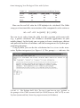
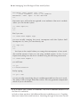
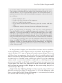
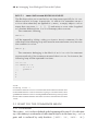
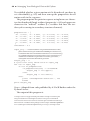
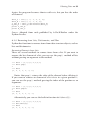
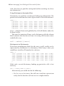
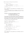
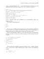
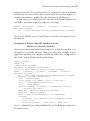
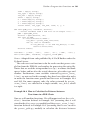
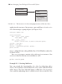
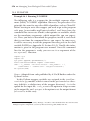
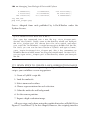
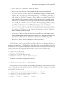
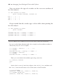
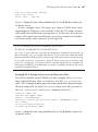
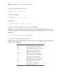
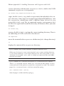
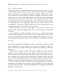
Importantly, the following Python session is meant to be written to a
file and executed (see Box 1.2 and Section 2.3.1). In the following, code
lines not preceded by the Python shell prompt >>> are meant to be written
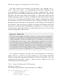
to a text file and executed (see Figure 2.1).
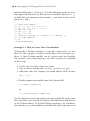
26 ◾ Managing Your Biological Data with Python
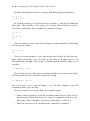
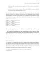
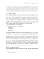
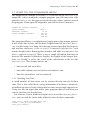
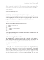
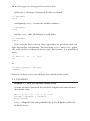
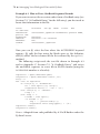
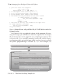
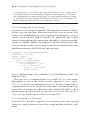
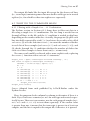
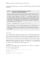
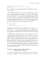
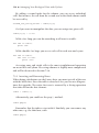
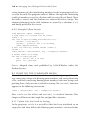
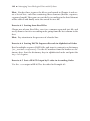
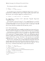
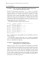
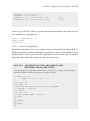
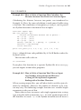
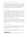
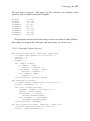
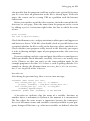
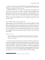
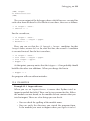
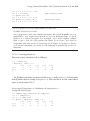
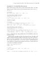
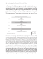
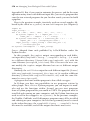
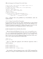
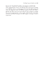
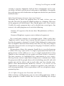
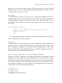
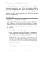
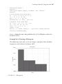
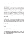
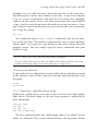
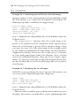
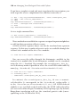
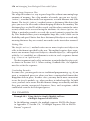
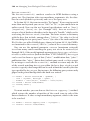
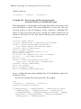
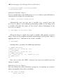
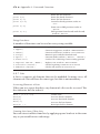
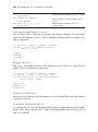
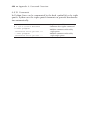
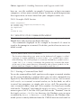
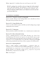
FIGURE 2.1 Text files and Python shell. Note: Left panel: A script written to a
text file. Right panel: The execution of the script in the Python shell.
2.2.2 Example Python Session
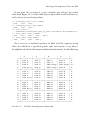
# insulin [Homo sapiens] GI:386828
# extracted 51 amino acids of A+B chain
insulin = "GIVEQCCTSICSLYQLENYCNFVNQHLCGSHLVEALYLVCGERGFFYTPKT"
for amino_acid in "ACDEFGHIKLMNPQRSTVWY":
number = insulin.count(amino_acid)
print amino_acid, number
Source: Adapted from code published by A.Via/K.Rother under the
Python License.
2.3 WHAT DO THE COMMANDS MEAN?
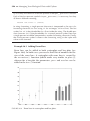
The program produces the following 20 × 2 table:
A
C
D
E
F
G
H
I
K
L
M
1
6
0
4
3
4
2
2
1
6
0
Your First Python Program ◾ 27 N
P
Q
R
S
T
V
W
Y
3
1
3
1
3
3
4
0
4
2.3.1 How to Execute the Program
When working on the Python shell, you had a window that was just for
entering commands. Where can you enter a program? Of course, you
could enter the above commands into the Python shell and they would
work. But then you would have to retype the program each time you want
to use it, including typing the insulin sequence!
A more convenient option is to store the program in a text file. Text files
can be opened using a text editor (see Box 2.2 and Box D.2). Text files containing Python programs should have the ending .py (the suffix may not
be visible). On Linux and Mac you can execute the Python program from
a terminal window by typing
python aa_count.py
BOX 2.2 TEXT EDITORS FOR PROGRAMMING
A text editor for programming must allow you to create files, write to
them, and save them on the hard disk. Examples of basic text editors are
Notepad++, Vim (http://www.vim.org/), TextEdit, Pico, and Gedit (http://
projects.gnome.org/gedit/). Most of them also highlight the syntax of
Python code automatically. When using a normal text editor, make sure
that tabs are automatically replaced by spaces. In Gedit you can configure
this in Edit => Preferences. Go to the Editor tab and check the box “Insert
spaces instead of tabs”.
The IDLE editor (automatically installed with Python on Windows) can
also recognize and manipulate code blocks (i.e., takes care of indentation).
On Linux and Mac OS X, iPython is an improved Python shell that not only
offers syntax highlighting of the code but also allows completion of many
functions by pressing the TAB key (see http://ipython.org/).
28 ◾ Managing Your Biological Data with Python
For Python there are several sophisticated editors, also called integrated
development environments or IDEs, that help you with several aspects of
programming. First, the editor helps to format the code consistently: adding spaces, highlighting keywords in different colors, highlighting missing
parentheses. Some IDEs even highlight syntax errors. While writing code,
you can look up names and documentation on the fly. While debugging you can go through the program step by step and trace the value of
variables without adding print statements. Popular Python IDEs are Eric
(Linux), SPE (Linux), and Sublime Text (Win/Mac/Linux, http://www.sublimetext.com).
On Windows, you can open the Python file in the IDLE editor (available
from ‘Start’ → ‘All Programs’ → ‘Python’ → ‘IDLE’, create a new file) and
press F5 to execute the program or select ‘Run’ → ‘Run Module’ from
the menu.
2.3.2 How Does the Program Work?
In the Python programming language, a program is executed one line after
the other. Each program line contains an instruction that tells the Python
interpreter what it has to do. What happens in aa_count.py in each line?
• # insulin. The first line does nothing. The hash # indicates that
this is a comment (see Section 2.3.3).
• insulin = "MALWM...". Here, the protein sequence is stored in a
variable called insulin. The protein sequence is defined as text, also
called a string (see Section 2.3.4). The backslash \ at the end of the line
indicates that the protein sequence continues on the next line.
• for amino_acid. This construction starts a loop going through
the 20 characters A, C, D, E... and repeats for each of them
the instructions in the next two lines. The name amino_acid is
a variable that contains a single character in each round. The loop
stops when the amino_acid variable reaches the last letter of the
"ACDEFGHIKLMNPQRSTVWY" string of characters.
• number = insulin.count(...). This calls a function that
calculates how often a character occurs in a piece of text, in
Your First Python Program ◾ 29 this case, the insulin protein sequence. The result is stored in a
variable.
• print amino_acid, number. This writes both the amino acid and
the result of the counting to the screen.
The last three lines form a code block. That means they are executed
together, in this case, 20 times because the for command repeats a block
of commands. The lines related to the for command are grouped by being
indented by four spaces. The effect of this block of code is the same as if the
program were written
number = insulin.count("A")
print "A", number
number = insulin.count("C")
print "C", number
number = insulin.count("D")
print "D", number
...
Thus, combining the loop with a block of commands helps avoid writing
a lot of redundant code.
In Python you normally have one instruction per line. However, long
instructions may span several lines, like the insulin sequence. In that case,
all but the last line need to end with a backslash character \:
>>> 3 + 5 + \
... 7
15
2.3.3 Comments
A comment is a portion of code that is addressed to other programmers
(or yourself when you read your program after days or weeks) and not to
the Python interpreter. In other words, it is a sort of documentation inside
the program used to describe what the code does. The text you want the
interpreter to ignore must be preceded by the # symbol.
>>> print "ACCTGGCACAA" # This is a DNA sequence
ACCTGGCACAA
30 ◾ Managing Your Biological Data with Python
2.3.4 String Variables
You saw in Chapter 1 that numbers can be stored in variables by simply
assigning a number to a variable name:
x = 34
Text variables contain a data type called string. In contrast to numbers,
strings in Python need to be enclosed by single ('abc'), double ("abc"),
or triple ('''abc''' or """abc""") quotes. For instance, to store the protein sequence of insulin in a variable named insulin, you need to use the
assignment operator =:
insulin = 'GIVEQCCTSICSLYQLENYCNFVNQHLCGSHLVEALYLVCGERGFFYTPKT'
>>> print insulin
GIVEQCCTSICSLYQLENYCNFVNQHLCGSHLVEALYLVCGERGFFYTPKT
Triple-quoted strings can span multiple lines (with no need for a backslash at the end of each line). This is useful to store longer pieces of text in
variables:
>>> text = '''Insulin is a protein produced in the pancreas.
The protein is cut proteolytically.
Its deficiency causes diabetes.'''
>>> print text
Insulin is a protein produced in the pancreas.
The protein is cut proteolytically.
Its deficiency causes diabetes.
Strings have an intrinsic order. When you run a for loop on a string, the
characters will always be processed in the same order. Strings are immutable objects. You cannot change single characters in an existing string
or replace a substring with another one; you can only create a new string.
Strings not only are useful for storing data but also provide a lot of powerful functions to manipulate and analyze text.
Indexing
By numerical indices in square brackets, you can extract characters in
certain positions. The first character is treated as in position zero:
>>> 'Protein'[0]
'P'
Your First Python Program ◾ 31 >>> 'Protein'[1]
'r'
Negative indices address characters starting from the end:
>>> 'Protein'[-1]
'n'
>>> 'Protein'[-2]
'i'
Slicing
By introducing a colon in the square brackets, you can address parts of the
string (slices). For instance [0:3] returns a substring starting at the beginning and stopping after the third character:
>>> 'Protein'[0:3]
'Pro'
The slice [1:] starts after the first character and stops at the end of the string.
>>> 'Protein'[1:]
'rotein'
String Arithmetics
Strings in Python can be added using the plus (+) operator. This simply
results in a concatenation of both strings.
>>> 'Protein' + ' ' + 'degradation'
'Protein degradation'
Strings can also be multiplied with integer numbers:
>>> 'Protein' * 2
'ProteinProtein'
>>> '*' * 20
'********************'
Determining String Length
The len() function returns the length of a string in number of characters:
>>> len('Protein')
6
32 ◾ Managing Your Biological Data with Python
Counting Characters
The s.count() function counts how often a character or a short sequence
occurs in a string:
>>> 'protein'.count('r')
1
More functions that work on strings can be found in Appendix A.
Q & A: WHY ARE SOME STRING FUNCTIONS LIKE count() ADDED
AFTER THE STRING WITH A DOT, AND OTHERS LIKE len() TAKE THE
STRING AS ARGUMENT?
Functions in Python are organized in several places. Some are so-called
built-in functions (like len()); you can use them anywhere without constraints. They are widely applicable; e.g., len() works on other data types
as well. Other functions are specific for certain data types; e.g., counting
in the way used in the program in Section 2.2.2 works for strings only. To
use count() you need to have a string first. Functions that are firmly connected to a certain type of object are also called methods of that object.
The assignment of methods to data types helps keep complicated programs
well organized. For more information on modular aspects of Python, see
Box 2.3 and Part III.
BOX 2.3 EVERYTHING IS AN OBJECT
Whenever you use a new piece of data in your program (numbers, text, or
more complex structures), the Python interpreter creates something called
an object. Each object has a reserved piece of memory where the data
is stored. A Python object also knows exactly what type of data it is. For
instance, if you assign a number to a variable
a = 1
Python creates an integer object somewhere in the computer memory.
The variable a points to that location in the memory. An object is also
created when you create a string variable. When you have a for loop,
each new value of the index variable is an object of its own as well. Each
object contains some data, but it can also contain functions that work
on data. The content of an object can be accessed by adding a dot to
the variable name; e.g., sequence.count('A') calls a method of the
sequence string variable.
Your First Python Program ◾ 33 Even a module that you import is an object. The math module, for
instance, contains data (e.g., math.pi) and functions (e.g., math.log).
Taken together, everything that you can give names to is an object, a container for both data and functions.
2.3.5 Loops with for
The control flow statement for is used for repeating actions. In particular,
the for statement makes it possible to execute instructions a given number of times. The for loop needs a sequence-like object (see Box 2.3): a
string it can go through character by character, a list of numbers that are
processed one by one, or simply a pile of data items that the loop works
through until the pile is empty. The elements of the sequence are made
available as an index variable. The instructions that are repeated are the
group of indented statements following the for instruction.
The general syntax of for loops is
for <index variable> in <sequence>:
<command 1>
<command 2>
...
<command x>
<sequence> may be a string ("ACDEFGHIKLMNPQRSTVWY") or a collection of objects such as a list ([1, 2, 3], explained in Chapter 4). <index
variable> is a variable name that takes the value of the elements of
<sequence> as it runs over its contents. In the first round, the index
variable has the first value of <sequence>; in the second round, it takes
the second value; and so on. The instructions <command 1> and <command 2> are executed during each round of the loop. They are marked as
belonging to the loop by being shifted right by four spaces (indentation).
The last instruction to be executed in a for loop is to be shifted by four
spaces. The instruction <command x> is executed as soon as the loop is
exited, i.e., it has finished with the last element of <sequence>.
Running a Loop over a String
When the sequence used in a for loop is a string, the code inside the loop
is repeated for each character:
for character in 'hemoglobin':
print character,
34 ◾ Managing Your Biological Data with Python
Source: Adapted from code published by A.Via/K.Rother under the
Python License.
For instance, the loop from the example program in Section 2.2.2 is run
20 times, one for each one-character amino acid code:
for amino_acid in "ACDEFGHIKLMNPQRSTVWY":
number = insulin.count(amino_acid)
print amino_acid, number
The number = insulin.count(amino_acid) and print amino_acid,
number statements are each repeated 20 times. In each round of the loop, the
amino_acid variable takes the value of the next character from the string
"ACDEFGHIKLMNPQRSTVWY". This way, each amino acid can be counted
without duplicating code. The loop stops when the amino_acid variable
has finished taking all the 20 values from the "ACDEFGHIKLMNPQRSTVWY"
string; in other words, when amino_acid equals “Y”, the for loop is executed one last time and then exits.
Running a Loop over a List of Numbers
A loop can simply print the contents of a list:
for i in [1, 2, 3, 4, 5]:
print i,
which results in:
1 2 3 4 5
A loop can use a function to create a sequence on the fly. For instance, the
built-in function range(10) creates a list of numbers from 0 to 9.
for number in range(10):
print number,
will result in:
0 1 2 3 4 5 6 7 8 9
2.3.6 Indentation
In the Python session in Section 2.2.2, not all code lines start at the same
point: two of them are preceded by a number of blank spaces. This is called
Your First Python Program ◾ 35 indentation and is used in Python to mark blocks of code that are executed
together.
Blocks of code occur in loops, conditional statements (see Chapter
4), functions (see Chapter 10), and classes (see Chapter 11). They all are
identified by indentation. A block of code is initiated by a colon character
and followed by the indented instructions of the block. The indentation
length of the first instruction of a block should be four spaces at least,
and all instructions of a block must be indented by the same number of
spaces. Although it is possible to use tabs for indentation, it is advised to
use spaces because tabs lead to problems in some text editors.
2.3.7 Printing to the Screen
The print command is a versatile way of displaying information on the
screen. It writes numbers and text to the text console. You can influence
the way the data are written in many ways. In the most straightforward
way, you simply print the data:
print 7
will print 7 to the screen of your computer, whereas
print 'insulin sequence:'
will simply print insulin sequence:.
Instead of the plain data, you can print a variable:
sequence = 'MALWMRLLPLLALLALWGPDPAAA'
print sequence
will create the output
MALWMRLLPLLALLALWGPDPAAA
You can print multiple values in one command by separating them
with commas:
print 7, 'insulin sequence:', sequence
will print
7 insulin sequence: MALWMRLLPLLALLALWGPDPAAA
36 ◾ Managing Your Biological Data with Python
By default, a line break (i.e., an end-of-line character) is added after
each print statement, so that
print 7, 'insulin sequence:'
print sequence
will print 7 and insulin sequence: in one line and the sequence in a
different line. Adding a comma at the end of the last item in the print
statement suppresses the line break. The following commands produce the
output in one line:
print 7, 'insulin sequence:',
print sequence
Escape Characters and Quotes
When printing text (or assigning it to a string variable) you cannot use
every character in a Python string. Some characters need to be replaced by
escape characters. For example, you need to write tabulators as \t (using a
backslash), newline characters as \n, and backslashes as \\.
Of course, you cannot use the same quotes in a string as the ones you
enclose the string in. If you enclose the string in single quotes, you can use
double quotes inside the string and vice versa; triple-quoted strings may
contain both:
print 'a single-quoted string may contain "".'
print "a double-quoted string may contain ''."
print '''a triple-quoted string may contain '' and "".'''
Both text and numbers can be formatted in more sophisticated ways, e.g.,
writing a fixed number of digits or right-justifying text (see Chapter 3). The
main advantage of the print command is that it is a straightforward way
to write any kind of information to the screen. Box 2.4 reports a list of the
new concepts introduced in Chapter 2.
BOX 2.4 NEW PYTHON CONCEPTS
•
•
•
•
•
Comments
String variables
for loops
Indentation
Print
Your First Python Program ◾ 37 2.4 EXAMPLES
Example 2.1 How to Create a Random Sequence
You can use a for loop for creating a random sequence (see also Recipe
2). The range() function allows you to repeat instructions a given
number of times. The random module allows you to create random
numbers. It provides a number of tools to manage random objects. For
example, the randint(i,j) function generates a number between i
and j with equal probabilities. In the following example program, a
random number (ten) and string indexing (AGCT) are used to create
a random sequence (of ten characters extracted from “AGCT”):
import random
alphabet = "AGCT"
sequence = ""
for i in range(10):
index = random.randint(0, 3)
sequence = sequence + alphabet[index]
print sequence
Source: Adapted from code published by A.Via/K.Rother under the
Python License.
In the first line, the random library is imported. The program
defines a string with the characters of the four nucleotides and assigns
it to the alphabet variable, then uses a for loop to randomly extract
10 times a character from alphabet and add it to the sequence
string, which starts empty (sequence = ""). The random extraction
is performed by taking letters from alphabet with random indices
generated by random.randint(). The program output is a random
sequence of 10 characters extracted from 'AGCT', for example,
GACTAAATAC
Notice that, being random, the output sequence will change each
time you execute the program.
Example 2.2 How to Run a Sliding Window over a Sequence
When you look for sequence motifs, it is often necessary to consider
all fragments of a sequence having a certain length. You can use a
for loop to create all possible subsequences of a given length from a
sequence:
38 ◾ Managing Your Biological Data with Python
seq = "PRQTEINSEQWENCE"
for i in range(len(seq)-4):
print seq[i:i+5]
Source: Adapted from code published by A.Via/K.Rother under the
Python License.
The variable i runs from zero to the length of the sequence minus
four; len(seq) is 15, thus range(11) produces all numbers from
0 to 10. The instruction seq[i:i+5] extracts a subsequence of 5
characters in length from the sequence at position i. Python starts
counting positions at zero; the first subsequence is from position 0 to
5, the last one from 10 to 14. Thus, the code produces
PRQTE
RQTEI
QTEIN
TEINS
...
WENCE
The range() function is described in detail in Chapter 4.
2.5 TESTING YOURSELF
Exercise 2.1 Frequency of Amino Acids in the Telomerase Protein
Sequence
In 2009, Elizabeth H. Blackburn, Carol W. Greider, and Jack W. Szostak
received the Noble Prize for discovering the function of the enzyme
telomerase, which is responsible for extending the ends of chromosomes.
Retrieve the 1,132-residue sequence of isoform 1 of human telomerase from the NCBI protein database. Which amino acid is the most
frequent?
Exercise 2.2 Frequency of Nucleotide Bases in a DNA Sequence
Change the program from Exercise 2.1 to count the frequency of the four
DNA bases instead. Test it first with a DNA sequence for which you know
the result, for instance, “AAAACCCGGT”. This approach makes it much
easier to discover small program errors.
Your First Python Program ◾ 39 Exercise 2.3 Print an Amino Acid Sequence One Residue at a Time
Write a program that prints the first amino acid of the insulin sequence,
then the first two, then the first three, and so on. You will need both the
range() and the len() functions.
Exercise 2.4 Removing Indentation
In the example program in Section 2.2.2 for counting amino acids,
replace the line
print amino_acid, number
with
print amino_acid, number,
Run the program again. Explain what happens.
Exercise 2.5 Twenty Commands or a for Loop?
The program for counting amino acids could simply consist of 20 commands for counting instead of the for loop:
number = insulin.count("A")
print "A", number
number = insulin.count("C")
print "C", number
number = insulin.count("D")
...
Would you prefer this implementation? Why or why not?
I SUMMARY
In Part I you learned all basic parts of the Python language. You can let
your computer execute actions, such as calculations. You know what a
variable is and how to use it comfortably; you also saw that data in Python
can be of different types such as integer or floating numbers, or string,
and that specific tools exist for working with different data types (e.g., the
function count() for strings). You met functions and saw how some of
them work. You also learned that some functions are built-in; i.e., they are
“universal” and may act on many different objects, and some others can
only apply to a specific object. For example, the function count() can
only be applied to string objects, and this is expressed by the “dot” syntax
(i.e., writing, for example, 'MALWMRLLPLLALLALWGPD'.count('L')).
Importantly, you learned that a program does not necessarily need to be
written in a single file but can be cleverly structured in several modules,
which can be connected to one another through the import statement.
In particular, Python provides literally hundreds of optimized modules
that other programmers wrote for you, such as math. Apart from Python
objects such as variables, functions, and modules, you also met a Python
control flow structure, the for loop, which turns out to be incredibly useful when you have to repeat things several times. It is made of the for
keyword, followed by a variable name (i, j, john, amino_acid, etc.)
running over a sequence, followed by a colon and a block of indented
code. So, you also learned what indentation is and what purpose it serves.
Finally, you have seen how to use the print statement to display your
result (or whatever text you want to display) on the computer screen.
41
II
Data Management
INTRODUCTION
In this part of the book, you will meet new data structures and control flow
structures. The data structures are lists (already mentioned in Chapter 2),
tuples, dictionaries, and sets. These structures make it possible to collect
and conveniently manipulate data. Some of them are more appropriate for
certain data and tasks than others, and it is up to you to choose the data
structure that best fits the problem at hand. Strings, lists, and tuples are
ordered collections of objects, whereas dictionaries and sets are unordered
collections of objects. If keeping the order is a priority, strings, lists, or
tuples are the appropriate structures to manage your data, but if you want
to extract specific elements from a large collection quickly or to determine
the intersection between two or more groups of objects, dictionaries and
sets are the right choice for you.
Here, you will also learn about two more control flow structures: if
conditions and while loops. The former makes it possible to execute a block
of instructions only if one or more conditions are met. It is a structure that
lets your program make decisions. The while loop combines the concepts
of for loops and if conditions. In fact, it makes it possible to repeat actions
until a given condition is verified. You can use it, for example, to read a
nucleotide sequence until you meet something weird like a non-nucleotide
character. All these new data and control flow structures are applied to
solve typical problems in computational biology such as manipulating sets
43
44 ◾ Managing Your Biological Data with Python
of numerical data, reading and writing sequence files, working with tables,
parsing sequence data records, selectively extracting information from sets
of data, sorting table columns, filtering and sorting data, or finding functional motifs in sequences or keywords in PubMed abstracts.
Chapter 3 is about data columns. It describes how to deal with sets
of data: how to read them from a text file, how to collect them in a data
structure and to manipulate them (e.g., convert them into floating numbers, add them, calculate their mean and standard deviation, etc.), and
how to write them to a text file. In Chapter 4 you will learn how to
extract information from sequence files, such as Uniprot, FASTA, or
GenBank nucleotide files. Chapter 5 shows how to use dictionaries to
store biological data and search them in a very quick manner. Chapter 6
shows ways to filter data by either combining loops with if statements
or using the set data type. Chapter 7 teaches how to read, organize,
manipulate, and write tabular data, for example, how to read a table in
tab-separated format, delete one of its columns, and write it to a new file
in comma-separated format. In Chapter 8, you will learn tricks for sorting your data, and in Chapter 9, you will see pattern matching tools, i.e.,
a syntax to encode a sequence consensus (e.g., extracted from a multiple
alignment), and a set of functions to search hits of the consensus in a
biological sequence.
The contents of Part I and Part II are the basics you need to repeat over
and over in order to become fluent in Python.
Chapter
3
Analyzing a Data Column
L
earning goal: You can calculate the average and standard deviation
from numbers in a text file.
3.1 IN THIS CHAPTER YOU WILL LEARN
• How to read numbers from a table
• How to read and write files
• How to calculate average values
• How to calculate a standard deviation
3.2 STORY: DENDRITIC LENGTHS
3.2.1 Problem Description
Neurobiological research studies, among other things, what conditions
make neurons grow. The growth of neuron cells can be analyzed by fluo
rescent microscopy. You obtain images in which you can measure the
dendritic arbor complexity. Software like Image J (Image Processing and
Analysis in Java, http://rsb.info.nih.gov/ij/) makes it possible to calculate
parameters like the dendritic length and to write the values to a text file.
Simplified, the file neuron_data.txt is a text file containing the length
of neurons in a single column of data:
16.38
139.90
441.46
45
46 ◾ Managing Your Biological Data with Python
29.03
40.93
202.07
142.30
346.00
300.00
If you need to work with such a set of numbers in a text file, there are several questions right at the beginning: How many measurements are there?
What is the longest dendritic length? What is the shortest? What is the
average length? What is the standard deviation? It would be great to see a
quick summary before analyzing the data in more detail.
If you have many files with measurements of the same kind, loading
all of them into Excel may be cumbersome. How can the data be read and
analyzed using Python? In the Python session in Section 3.2.2, you will see
a function that opens a file for reading or writing, open(filename, option).
It generates a Python file object, which can be read or written, depending
on whether option is 'r' (= read) or 'w' (= write), respectively. To write
text to a file, you can use write(some_text). write() is a method of file
objects, and as such, you have to use the dot syntax to write something to
a file. In Section 3.2.2, a for loop is used to read line by line the file object
returned by the open(filename)function.
3.2.2 Example Python Session
data = []
for line in open('neuron_data.txt'):
length = float(line.strip())
data.append(length)
n_items = len(data)
total = sum(data)
shortest = min(data)
longest = max(data)
data.sort()
output = open("results.txt","w")
output.write("number of dendritic lengths : %4i \n"%(n_items))
output.write("total dendritic length : %6.1f \n"%(total))
output.write("shortest dendritic length
: %7.2f \n"%(shortest))
output.write("longest dendritic length
: %7.2f \n"%(longest))
output.write("%37.2f\n%37.2f"%(data[-2], data[-3]))
output.close()
Source: Adapted from code published by A.Via/K.Rother under the Python
License.
Analyzing a Data Column ◾ 47 3.3 WHAT DO THE COMMANDS MEAN?
The output of the example in Section 3.2.2 is written to the results.txt
output file. After running the example program, you will notice that a file
named results.txt has appeared in the directory where you have started
the program. If you open the output file, you will see that its content is
number of neuron lengths
total length
shortest neuron
three longest neurons
:
9
:1658.1
: 16.38
: 441.46
346.00
300.00
The program follows a straightforward input-processing-output pattern.
It first reads, line by line, the dendritic lengths from the neuron_data.
txt text file using a for loop. After having removed possible blank spaces
and newline characters (line.strip()), it converts each line (i.e., each
neuron length) into a floating-point number and adds it to the data list
(data.append(length)). Then, it uses a couple of built-in functions to
measure the number of dendritic lengths, the length of the longest dendrite, etc. Finally, it writes the result of the calculations to the text file
results.txt. This chapter focuses on
• how to read and write files,
• how table columns are read to lists of numbers, and
• how lists of numbers can be evaluated.
3.3.1 Reading Text Files
A small number of data items can be written directly into the Python
code. This is also called hard-coding information. For dozens, hundreds,
or millions of entries, hard-coding data becomes increasingly impractical.
Using text files for input data makes your program shorter, and often you
can use the files you already have.
For instance, if your dendritic lengths are in a text file neuron_data.
txt, you can read the entire body of data by three Python commands:
text_file = open('neuron_data.txt')
lines = text_file.readlines()
text_file.close()
48 ◾ Managing Your Biological Data with Python
Source: Adapted from code published by A.Via/K.Rother under the
Python License.
The program does three things:
1.
Opens a text file. The file is specified by a filename in the form of a
string (between single or double quotation marks). It is assumed that
the file is in the same directory as your Python program. Otherwise,
you would need to add the directory path before the filename.
2.
Reads the dendritic lengths from the file. The readlines() function simply reads everything that is in the file line by line and
stores each line in a separate string. The strings are returned as a
list of strings. In contrast, read() reads the entire file into a single
string.
3.Closes the text file. It is good practice to close files that you open.
Python closes files automatically as soon as your program terminates, but if you try to open the same file a second time without closing it before, you ask for trouble.
Many programs, like the Python session in Section 3.2.2, that read data
from a text file will contain two lines similar to the following:
for line in open(filename):
line = line.strip()
The first line opens the file for reading and runs a for loop over each line.
This line is shorter than using the readlines() function on a file, but it
does not create a list variable. The second line will be repeated for each line
of the file. The strip() function removes blank spaces at the beginning
and at the end of a line (if present) and the newline character from the end
of the line. After that, the data are ready to be used.
3.3.2 Writing Text Files
Analogously, you can write the output of your program to a file instead of
to the screen. This way, you can write the results to a spreadsheet or simply
save them for later. In Python, a file is written by
output_file = open('counts.txt', 'w')
output_file.write('number of neuron lengths: 7\n')
output_file.close()
Analyzing a Data Column ◾ 49 Source: Adapted from code published by A.Via/K.Rother under the
Python License.
This code does the following:
1.
Opens a text file for writing. This differs from the usage of open()
you used for reading by the 'w' character (w = write). A file opened
with the 'w' flag can be used only for writing.
2.Writes a string to the file. The write() function accepts only
string data, so you need to convert to a string whatever you want
to write. We will explain converting numbers to strings later. Note
that the previous string ends with a newline character (the \n),
because write() does not introduce line breaks automatically, so
you have to add them explicitly if you need them. Alternatively, the
writelines() function accepts a list of lines (each in the form of
a string).
3.
Closes the file after usage. Tidying up after finishing the work is good
programming style. If you forget to close the file, nothing dangerous happens (your data are not lost). Python does that automatically
when the program execution is over. However, it can lead to problems if you use the same file again:
>>>
>>>
>>>
>>>
''
f = open('count.txt','w')
f.write('this is just a dummy test')
g = open('count.txt')
g.read()
Why is the file empty? Where did the text go? It is still “floating” in the
computer memory. In fact, strings are actually saved to files only when
a certain number of characters has been reached (i.e., they are buffered).
However, when you close the file, the data will be saved in any case, no
matter how many characters you have written. Therefore, a better way to
write the code is
>>> f = open('count.txt','w')
>>> f.write('this is just a dummy test')
>>> f.close()
>>> g = open('my_file')
>>> g.read()
'this is just a dummy test'
>>>
50 ◾ Managing Your Biological Data with Python
Source: Adapted from code published by A.Via/K.Rother under the
Python License.
3.3.3 Collecting Data in a List
To work with the entire set of dendritic lengths, you need to put the data
somewhere. The program uses a Python list for that. Lists in Python are
containers for collections of data with arbitrary length. In the program, an
empty list is created at the beginning:
data = []
In the for loop, the neuron lengths from the text file are converted to
float numbers and then added to the list:
data.append(float(length))
The for loop in the previous program reads all neuron lengths from the
text file into a single list variable. The content of the list after the loop is
data= [16.38, 139.90, 441.46, 29.03, 40.93, 202.07, 142.30, \
346.00, 300.00]
Lists are one of the most powerful data structures in Python. The main
advantage of using a list is that you can store an entire data set into a single
variable. You don’t even have to know the number of items in advance: the
list grows automatically. You can use lists in a for loop and with many
functions that evaluate data. Lists will be covered in more depth in the
next chapter.
3.3.4 Converting Text to Numbers
When the program is reading the neuron lengths from the text file, they
are string variables at first. To do calculations, however, the program must
work with floating-point or integer numbers. In Python, you can convert
a string to a floating-point number with float():
number = float('100.12') + 100.0
which gives a totally different result (200.12) than
number = '100.34' + '100.0'
Analyzing a Data Column ◾ 51 which results in '100.34100'. The conversion from strings to numbers
results in an error if the text makes no sense numerically; for example,
float('hello')
returns the following error:
ValueError: invalid literal for float(): hello
In fact, hello is a string that cannot be converted to a number. It does not
make any difference whether you convert a string that is hard-coded in the
program (like above) or is assigned to a variable like in the line
length = float(line.strip())
You can convert floats to integer and vice versa.
>>> number = int(100.45)
>>> number
100
>>> f_number = float(number)
>>> f_number
100.0
When converting to integer, the number may contain decimal places, but
they will be truncated.
3.3.5 Converting Numbers to Text
For information to be written to a text file, it must be in the form of a
string. Both integer and float numbers (and every other type of data) can
be converted to a string using the same function for the conversion:
>>> text = str(number)
>>> text
'100'
Using the str() function to convert numbers has a big disadvantage,
however: the numbers in the text file will be unformatted. You cannot
align numbers to occupy a given number of columns. Especially float
numbers will have many decimal places that make your output less readable. An alternative to str() is to use string formatting. You can insert
52 ◾ Managing Your Biological Data with Python
integer numbers into a string by using a percent character indicating the
number of places you want to allocate for the integer:
>>> 'Result:%3i' % (17)
'Result: 17'
The %3i indicates that the string should contain an integer formatted to
three positions. The actual value for the integer comes from the parentheses at the end. In the same way, you can insert floating-point numbers
into a string with %x.yf, where x is the number of total characters (also
counting the dot) and y is the number of decimal places.
>>> '%8.3f' % (12.3456)
' 12.346'
You can also format strings with %s:
>>> name = 'E.coli'
>>> 'Hello, %s' % (name)
'Hello, E.coli'
Normally, %s simply inserts the string, but you can also right-justify it
by, e.g., %10s or left-justify it by %-10s. Multiple values can be inserted
at the same time, and text between the formatting characters is allowed.
Then, you need to take care to provide the exact number of values to insert
at the end:
'text:%25s numbers:%4i%4i%5.2f' % ('right-justified', 1, 2, 3)
'text:
right-justified numbers: 1 2 3.00'
Summarizing, the string formatting in Python is a powerful option to create
neatly formatted output from your data.
3.3.6 Writing a Data Column to a Text File
When your program has finished calculations, you may want to write the
results to a text file. If your result is a list of numbers, you can format them
to a list of strings and then pass the list to the writelines() method of file
objects:
data= [16.38, 139.90, 441.46, 29.03, 40.93, 202.07, 142.30, \
346.00, 300.00]
out = []
Analyzing a Data Column ◾ 53 for value in data:
out.append(str(value) + '\n')
open('results.txt', 'w').writelines(out)
Source: Adapted from code published by A.Via/K.Rother under the
Python License.
The for loop goes through each value of the list, converts it to a string,
and adds a newline character ('\n'). The values are collected in a list
of strings that is written to a file at the end of the script. Note that, as
mentioned earlier, for writing a list of strings into a file, you can use the
writelines() function.
If you prefer to format the result as a long single string, the loop looks
slightly different:
out = []
for value in data:
out.append(str(value))
out = '\n'.join(out)
open('results.txt', 'w').write(out)
The '\n' join() function connects all values to a single string by newline
characters, so that write() can be used. Notice that you can use join()
to glue any number of strings together, connecting them by a linker string
(a newline character '\n' in the previous example):
>>> L = ['1', '2', '3', '4']
>>> '+'.join(L)
'1+2+3+4'
The result is a string.
3.3.7 Calculations on a List of Numbers
A list of numbers is a powerful structure for your data. You can use a list as
you would a column in a spreadsheet. Python has a set of built-in functions for
working with lists of numbers and strings. Given the dendritic lengths in a list
>>> data = [16.38, 139.90, 441.46, 29.03, 40.93, 202.07, 142.30, \
346.00, 300.00]
the len() function returns the length of the list, i.e., the number of items
in the list:
>>> len(data)
9
54 ◾ Managing Your Biological Data with Python
With max() the largest element of the list is returned:
>>> max(data)
346.0
Analogously, min(), returns the smallest number:
>>> min(data)
16.38
Finally, sum() adds all elements to each other:
>>> sum(data)
1658.0
You can print the results of these operations or put them into variables for further calculations. The functions min() and max() generally work on lists of elements of any type. For instance it is possible to
write:
>>> max(['a', 'b', 'c', 'd'])
'd'
or
>>> max(['Primary', 100.345])
'Primary'
however, in these cases, you will have less control on the result.
3.4 EXAMPLES
Example 3.1 How to Calculate a Mean Value
Assume you have measured five dendritic lengths and want to know
their mean value:
data = [3.53, 3.47, 3.51, 3.72, 3.43]
average = sum(data) / len(data)
print average
Source: Adapted from code published by A.Via/K.Rother under the
Python License.
Analyzing a Data Column ◾ 55 In the first line, all five measurements are put into a list and stored
in the variable data. In the second line, the arithmetic mean is calculated using the formula
1
µ=
N
N
∑x
i
i =1
The sum() function adds up all values in the list data.
>>> sum(data)
17.66
The len() function gives the number of items in the list (its length).
>>> len(data)
5
By using the combination of len() and sum(), you can calculate
the arithmetic mean of any list that is not empty. You don’t have to
know how many items are inside at the time you write the program.
If your data consist of integer numbers, the result will be rounded
down by default. If you prefer to see an average with decimal places,
you need to convert the sum or length to a float:
data = [1, 2, 3, 4]
average = float(sum(data)) / len(data)
print average
Source: Adapted from code published by A.Via/K.Rother under the
Python License.
When one of the numbers of the division is a float, the result will
be a float as well.
Example 3.2 How to Calculate a Standard Deviation
Calculating a standard deviation is a little more complicated, because
you need a for loop to calculate the square difference for each value.
It is necessary to have the average calculated previously. Then, for
each value, you have to subtract the average and square the result
((value – average) ** 2). All squared differences must be added
56 ◾ Managing Your Biological Data with Python
together and the result divided by the total number of values. Finally,
you have to calculate the square root of the result. To add together
the squared differences, you can set a variable to 0.0 and add the
squared difference for each value to it.
The formula for the standard deviation is
1
σ=
N
N
∑( x − µ )
i
2
i =1
and the script that calculates it is
import math
data = [3.53, 3.47, 3.51, 3.72, 3.43]
average = sum(data) / len(data)
total = 0.0
for value in data:
total += (value - average) ** 2
stddev = math.sqrt(total / len(data))
print stddev
Source: Adapted from code published by A.Via/K.Rother under the
Python License.
Example 3.3 How to Calculate a Median Value
Another useful measure is the median, the value dividing a data set
in two equal halves. To calculate the median from a list of numbers,
it is necessary to sort the data. Depending on whether the number of
elements is odd or even, the calculation differs slightly:
data = [3.53, 3.47, 3.51, 3.72, 3.43]
data.sort()
mid = len(data) / 2
if len(data) % 2 == 0:
median = (data[mid - 1] + data[mid]) / 2.0
else:
median = data[mid]
print median
Source: Adapted from code published by A.Via/K.Rother under the
Python License.
Analyzing a Data Column ◾ 57 The function data.sort() sorts the data in ascending order (see
Chapter 8 for details). The if statement (explained in Chapter 4) is used
to distinguish between lists where the length can be divided by two and
odd lengths. Finally, the square brackets, e.g., data[mid], are used to
access individual elements of the list (also explained in Chapter 4).
3.5 TESTING YOURSELF
Exercise 3.1 Read and Write a File
Write a program that reads the file with neuron lengths and saves an identical copy of the file.
Exercise 3.2 Calculate Average and Standard Deviation
Extend the example in Section 3.2.2 so that it calculates the average neuron length and standard deviation.
Exercise 3.3 Frequency of Nucleotides
Write a program that reads a DNA sequence from a plain text file. Count
the frequency of each base. The program has to determine how often the
most frequent base occurs.
Hint: You don’t have to identify which base it is.
Exercise 3.4 GC-Content from a DNA Sequence
Write a program that calculates the GC-content of a DNA sequence from
a plain text file.
Exercise 3.5
Write the results of Exercises 3.3 and 3.4 to a text file.
Chapter
4
Parsing Data Records
L
earning goal: You can extract information from text files.
4.1 IN THIS CHAPTER YOU WILL LEARN
• How to integrate mass spectrometry data into metabolic pathways
• How to parse sequence FASTA files
• How to parse GenBank sequence records
4.2 STORY: INTEGRATING MASS SPECTROMETRY
DATA INTO METABOLIC PATHWAYS
4.2.1 Problem Description
To parse data files, you need to know two things: how to use lists to collect
data, and how to make decisions in your program in order to extract the
data you want. In this chapter, you will first meet these two central elements of the Python language in a simple example. Then, you will be ready
to parse a couple of real biological data files in Section 4.4.
Suppose you want to identify proteins belonging to a given metabolic
or regulatory pathway (e.g., cell cycle) that are expressed in a given cancer cell. Your initial data set may be represented by (1) a list (list_a) of
proteins (in the form of, e.g., Uniprot ACs) participating in the cell cycle
that you read from a text file (file_a) and (2) a second list (list_b)
of proteins that have been detected in a given cancer cell by means of,
e.g., a mass spectrometry experiment and that you read from a second
59
60 ◾ Managing Your Biological Data with Python
text file (file_b). Such text files can be downloaded from resources like
Reactome (see Box 4.1) or can be the result of your experiments. In both
cases, you need to read the data into your program before you can compare the two lists. File formats easily readable by a script are csv (commaseparated values) or tsv (tab-separated values), but a simple text file (as
those in Section 4.2.2) with protein identifiers would be appropriate as
well (see Box 4.1).
BOX 4.1 MASS SPECTROMETRY
Mass spectrometry (MS) is a technique used to determine the elemental
composition of a sample of molecules. This technique can be used for
the characterization and sequencing of proteins, and, as such, MS-based
proteomics can be applied to obtain comprehensive pictures of gene
expression. In this sense, the very final output of an MS experiment basically consists of a list of peptides that have been detected (i.e., that are
expressed) in a sample under study. Thanks to the availability of specific
data analysis software (e.g., Mascot, http://www.matrixscience.com/), MS
peptides can be matched against Uniprot sequences so that the output list
can be available in the form of Uniprot IDs and typically stored to a csv
(comma-separated values) text file:
protein_hit_num,prot_acc,prot_score,prot_matches
1," P43686",194,15
2," P62333",41,4
…
As for metabolic pathways, several resources are freely available on the
Internet. Reactome (http://www.reactome.org/) is one of these. If you click
on the Browse Pathways link on the Reactome website, you can select an
organism and a pathway and download a list of proteins participating in
that pathway in a format of your choice, e.g., textual:
Uniprot ID
P62258
P61981
P62191
P17980
P43686
P35998
P62333
Q99460
O75832
…
Parsing Data Records ◾ 61 Once MS data have been read, the problem of integrating the data into a
pathway comes down to the problem of printing all proteins from list_a
that are also in list_b, which is a pretty simple task.
4.2.2 Example Python Session
# proteins participating in cell cycle
list_a = []
for line in open("cell_cycle_proteins.txt"):
list_a.append(line.strip())
print list_a
# proteins expressed in a given cancer cell
list_b = []
for line in open("cancer_cell_proteins.txt"):
list_b.append(line.strip())
print list_b
for
protein in list_a:
if protein in list_b:
print protein, 'detected in the cancer cell'
else:
print protein, 'not observed'
Source: Adapted from code published by A.Via/K.Rother under the
Python License.
The output of the script is
P62258
P61981
P62191
P17980
P43686
P35998
P62333
Q99460
O75832
not observed
not observed
not observed
not observed
detected in the cancer cell
not observed
detected in the cancer cell
not observed
not observed
4.3 WHAT DO THE COMMANDS MEAN?
In the Python session in Section 4.2.2, two small lists of proteins are
read from text files and compared. In the program, you can recognize a
for loop and a list data structure, which were introduced in Chapters 2
and 3. The two lists both contain Uniprot ACs and have been assigned
to the list_a and list_b variables. Finally, there is a new language
construct, the if … else … clause. It is used to make decisions inside the
program. Both if ... else clauses and lists are essential to parse files more
62 ◾ Managing Your Biological Data with Python
complicated than a simple list of protein identifiers. If you are planning to
write your own parsers, it is worth it to get comfortable with both of these
Python structures first. This will make it a lot easier to combine them in
the right way in your own programs.
4.3.1 The if/elif/else Statements
Parsing a data record essentially consists of reading the record line by
line ("for line in file_a:"), as you learned in the previous chapter,
selecting from each line the information relevant to you and loading it
into a data structure (list_a.append(line.strip())) if you need to
further manipulate it or copying it to a new file if you want to store it
for future use. To extract specific parts from a line of text, you need to
execute a set of statements only on certain conditions (e.g., you may want
to print a Uniprot AC from a list only if it is also present in another list).
Here, we will explain how to do this, i.e., how to make choices using
Python.
The structure to be used is the following:
if <condition 1>:
<statements 1>
[elif <condition 2>]:
<statements 2>]
[elif <condition 3>]:
pass]
…
[else:
<statements N>]
The elif (else + if) and else statements and the corresponding blocks
of instructions are optional.
In the previous example, the following instruction
for item in list_a:
makes the index item run over the objects listed in list_a (i.e., Uniprot
ACs in cell cycle), and for each value taken by the index item, the following commands are carried out:
if item in list_a:
print item, 'detected in the cancer cell'
else:
print item, 'not observed'
Parsing Data Records ◾ 63 In other words, if a Uniprot AC from list_a is also found in list_b, it
will be printed followed by the string 'detected in the cancer cell';
otherwise it will be printed followed by the string 'not observed'.
This can be restated as follows: if the condition item in list_b is
true, print the item followed by the string 'detected in the cancer
cell'; otherwise print the item followed by the string 'not observed'.
To formulate conditions in if clauses, you need special operators to
compare numbers and objects and, for example, to verify if they are equal
(==) or different (!= or <>), if one is greater than the other or vice versa
(<, <=, >=, >), if one is contained in the other or not (in, not in), and if one
is the other or not (is, is not). For comparison operators, also see Box 4.2.
What all expressions used in if clauses have in common is that they
will result in one of two possible values: True or False. These two possible logical values are a data type called Boolean (named after George
Boole). If the returned value is True, the corresponding block of statements will be executed; otherwise it will not.
You can also verify if two or more conditions are met together or alternatively. The three Boolean operators and, not, or make it possible to
combine conditions:
seq = "MGSNKSKPKDASQRRRSLEPAENVHGAGGGA\
FPASQTPSKPASADGHRGPSAAFAPAAAE"
if 'GGG' in seq and 'RRR'in seq:
print 'GGG is at position: ', seq.find('GGG')
print 'f'RRR is at position: ', seq.find('RRR')
if 'WWW' in seq or 'AAA' in seq:
print 'Either WWW or AAA occur in the sequence'
if 'AAA' in seq and not 'PPP' in seq:
print 'AAA occurs in the sequence but not PPP'
Source: Adapted from code published by A.Via/K.Rother under the
Python License.
Q & A: HOW CAN I USE THE elif STATEMENT?
elif stands for else if, and it is used to test a condition only if all conditions of the preceding if/elif statements are not satisfied. Here, we identify numbers in the range 0–30 that are not divisible by 2, 3, 5 and therefore
are prime numbers (this is true for numbers in the range 4–30). The order of
the if/elif statements matters; the first condition that applies is taken. This
is why we first need to check whether a number is less than 4, because 2 and
3 are divisible by 2 and 3 yet they are prime numbers.
64 ◾ Managing Your Biological Data with Python
BOX 4.2 OPERATORS USED IN if CONDITIONS
If a condition returns the Boolean value True, the statements in the corresponding block will be executed. If it returns the Boolean value False,
the statements in the corresponding block will be ignored.
Condition
A<B
A lower than B
A <= B
A lower than or equal to B
A>B
A greater than B
A >= B
A greater than or equal to B
A == B
A equal to B
A != B
A different from B
A <> B
A different from B
A is B
A is the same thing as B
A is not B
A is not the same thing as B
A in B
A is present in the sequence B
A not in B
Example
Boolean
Value
3<5
5<3
(1 + 3) <= 4
4 <= 3
3*4 > 2*5
10 > 12
10/2 >= 5
5 >= 2
'ALA' == 'ALA'
'ALA' == 'CYS'
'ALA' != 'CYS'
'ALA' != 'ALA'
'ALA' <> 'CYS'
'ALA' <> 'ALA'
'ALA' is 'ALA'
'ALA' is 'CYS'
'A' is not 'C'
'A' is not 'A'
'A' in 'ACTTG'
'U' in "ACTTG"
"U" not in "ACTTG"
"A" not in "ACTTG"
True
False
True
False
True
False
True
False
True
False
True
False
True
False
True
False
True
False
True
False
True
False
Meaning
A is not present in the sequence B
In conditions, the number 1 and nonempty objects (e.g., a nonempty
string) correspond to the Boolean value True, and 0 and empty objects
(e.g., an empty string '' or an empty list []) correspond to the Boolean
value False. For example,
>>> if 1:
... print 'This is True'
...
This is True
>>> if '':
... print 'Nothing will be printed'
...
>>>
Parsing Data Records ◾ 65 for i in range(30):
if i < 4:
print "prime number:", i
elif i % 2 == 0:
print "multiple of two:", i
elif i % 3 == 0:
print "multiple of three:", i
elif i % 5 == 0:
print "multiple of five:", i
else:
print "prime number:", i
Source: Adapted from code published by A.Via/K.Rother under the
Python License.
Q & A: IS THERE A LIMIT ON THE NUMBER OF ELIF STATEMENTS THAT
I CAN USE?
No, but keep in mind that as soon as one condition is met, all subsequent
elif statements in the same if/elif/else block will be ignored by the
Python interpreter. Moreover, you can use the else statement only once in
an if/elif/else block. It will be executed provided that none of the preceding conditions have been met.
4.3.2 List Data Structures
Python provides three data structures to work with sequences of items
(i.e., ordered collections of objects): strings, tuples, and lists. You met
strings in Chapter 2, and in Chapter 3 lists were introduced to store a
set of strings and a set of numbers. However, lists can do a lot more.
They are very powerful and versatile tools to manipulate any kind of
data.
A list is an ordered mutable set of objects (strings, numbers, lists, etc.)
enclosed in square brackets. The fact that lists are mutable means that they
can be modified at any moment, i.e., new elements can be added, and elements can be replaced or removed altogether. The elements of a list can be
any kind of object (numbers, strings, tuples, other lists, dictionaries, sets,
or even functions [to be introduced in later chapters]) or a blend of different objects.
For instance,
>>> list_b = ['P43686', 'P62333']
66 ◾ Managing Your Biological Data with Python
is a list of strings, whereas
>>> list_c = [1, 2.2, 'P43686', [1.0, 2]]
is a list made up of an integer, a floating number, a string, and a list.
Other examples of lists include the following:
>>> d1 = []
>>> d2 = [1, 2, 5, -9]
>>> d3 = [1, "hello", 12.1, [1, 2, "three"], "seq", (1, 2)]
The first one is an empty list, which is useful for collecting data later in
a program. The last list d3 also includes a tuple, which is defined by round
brackets (see Box 4.3).
BOX 4.3 TUPLES
Tuples are immutable ordered sequences of objects and are indicated with
round brackets, (a, b, c), or by simply listing the sequence of items separated by commas: a, b, c. This implies that once you have defined a tuple,
you cannot change or replace its elements.
data = (item1, item2, item3,…)
Notice that brackets are optional; i.e., you can use either data =
(1,2,3) or data = 1,2,3
A tuple of a single item must be written either
data = (1,) or data = 1,
The operations of indexing and slicing are allowed also with tuples:
>>> my_tuple = (1,2,3)
>>> my_tuple[0]
#indexing
1
>>> my_tuple[:]
#slicing
(1, 2, 3)
>>> my_tuple[2:]
#slicing
(3,)
>>> my_tuple[0] = 0 #reassigning (Forbidden)
Traceback (most recent call last):
File "<stdin>", line 1, in <module>
TypeError: 'tuple' object does not support item assignment
Parsing Data Records ◾ 67 Like strings, lists support indexing and slicing operations (see
Chapter 2). With reference to the list d3, we can use indexing to extract
the first element of the list:
>>> d3[0]
1
Or we can use slicing to generate a list containing the third-to-the-last element of the original list:
>>> d3[2:]
[12.1, [1, 2, "three"], "seq", (1, 2)]]
Notice that, similarly to strings, the index of the first element of a list
is 0. You can also count from the last element using negative integers, so
that, for example,
>>> d2[–1]
-9
Sometimes you will see two indices with square brackets:
>>> d3[3][2]
"three"
What is happening here? The instruction selectively fished the third element ("three") of the fourth element ([1,2,"three"]) of the list (this is
possible because lists can contain other lists).
Notice that
L[i][j]
is actually the element of a table (or matrix) corresponding to the ith row
and jth column. Lists of lists are called nested lists and are the Python
way to represent and manipulate tables. Nested lists are discussed in more
detail in Chapter 7.
Even more brackets are possible:
>>> d3[3][2][0]
"t"
This command selected the first element ("t") of the third element
("three") of the fourth element ([1,2,"three"]) of the list. The first two
68 ◾ Managing Your Biological Data with Python
pairs of square brackets address elements of lists; the last picks a single
character ("t") from a string ("three").
A complete list of operators and methods common to strings, tuples,
and lists is reported in Appendix A.
Lists Are Mutable Objects
In contrast to strings and tuples, which are immutable objects, lists can be
modified (see Appendix A, Section A.2.7, “Lists,” subsection “Modifying
Lists”). This makes them very flexible objects. For example, you can reassign any element of a list:
>>> data = [0,1,2,3,4]
>>> data[0] = 'A'
>>> data
['A', 1, 2, 3, 4]
In this case, the first element of the list is replaced. When you reassign
one of its items, you can see that the original list changes. In other words,
you did not create a new list but rather modified the original one, which
does not exist anymore in its original form.
Some of the actions that can be performed on lists are carried out by
specific methods:
>>>
>>>
>>>
[0,
data = [0,1,2,3,4]
data.append(5)
data
1, 2, 3, 4, 5]
The method append() adds the item in brackets (the number 5 in this
case) to the end of the list. It is a method of the list object (i.e., a function acting only on lists), and as such, you have to use the dot (see also
Chapter 1 and Box 1.4) to link it to “its” object. The list (data) contains
the append() method in a similar way as the math module contains the
sqrt() function (see Chapter 1).
The dot is a “linker” between two objects. In this case the first of the two
objects is a list (data), and the second object is a function (append()).
When a function refers to a specific object, it is called a method of that
object. So, we can say “the method append() of the list data.” This concept, as you will also see later in this book, applies to all kinds of objects,
so we can talk about methods of modules (e.g., math.sqrt()) or methods
of classes (see Chapter 11).
Parsing Data Records ◾ 69 4.3.3 Concise Ways to Create Lists
Creating a List of Consecutive Numbers
If you want to generate an ordered list of integers, you can use the function
range(i). i is the number of integers generated by the function.
>>> range(3)
[0, 1, 2]
This may turn out to be very useful when you want to execute a for
loop running over a very long list of ordered integers. The built-in function
range() will be described in detail in Chapter 10 (in particular, see Box 10.3).
Creating a List of Zeroes
Sometimes it is useful to have a list that contains just a given number of
zeroes (or some other numbers). Instead of writing a for loop, you can use
the multiplication operator:
data = [0.0] * 10
List Comprehension
Another way to concisely generate lists is the list comprehension. It basically consists of putting between square brackets (1) a variable (e.g., x), (2)
the set of values taken by the variable (e.g., x in range(5)), and (3) an
expression (e.g., x**2) defining the values of the list elements.
>>> data = [x**2 for x in range(5)]
>>> data
[0, 1, 4, 9, 16]
In the following example, a new list data is created by running the
variable base in the seq string and including an element in data only if
it is also present in the bases list:
bases = ['A', 'C', 'T', 'G']
seq = 'GGACXCAGXXGATT'
seqlist = [base for base in seq if base in bases]
print seqlist
Source: Adapted from code published by A.Via/K.Rother under the
Python License.
The code results in:
['G', 'G', 'A', 'C', 'C', 'A', 'G', 'G', 'A', 'T', 'T']
70 ◾ Managing Your Biological Data with Python
4.4 EXAMPLES
With the if … elif construct and the list data type explained, it is time
to look at some real file parsers. In the following examples, you will see
how to read the content of a protein sequence FASTA file line by line
(see Appendix C, Section C.1, “A Single Protein Sequence File in FASTA
Format,” and Section C.2, “A Single Nucleotide Sequence File in FASTA
Format”) and make choices by means of the if/elif/else construct.
You can download the sample files by going to the Uniprot website (http://
www.uniprot.org/), access the entry of a protein of your choice, and click
on the “fasta” link. Then, you can copy and paste the FASTA-formatted
sequence to a local text file. To create a multiple sequence file, you can
repeat this procedure several times (or download from the Uniprot website the entire SwissProt data set in FASTA format).
Example 4.1 Read a Sequence File in FASTA Format and
Write Only the Sequence Header to a New File
Each sequence record in a FASTA file is composed of two parts: a
header line and the 64-character-long sequence line(s) (the number of which depends on the sequence length). The header line is
marked by a greater than symbol (>) at the first position of the line,
and you can use it to distinguish this line from the ones with the
sequence.
fasta_file = open('SwissProt.fasta','r')
out_file = open('SwissProt.header','w')
for line in fasta_file:
if line[0:1] == '>':
out_file.write(line)
out_file.close()
Source: Adapted from code published by A.Via/K.Rother under the
Python License.
Example 4.2 How to Extract a List of Accession Codes
from a Multiple Sequence FASTA File
How were the input data files for the Python script in Section 4.2.2
created? Consider SwissProtSeq.fasta, a FASTA file of the form
Parsing Data Records ◾ 71 reported in Appendix C, Section C.4, “A Multiple Sequence File in
FASTA Format.” The accession codes may originate from the header
lines like the following, enclosed by the pipe symbol ‘|’:
>sp|
P03372|ESR1_HUMAN Estrogen receptor OS = Homo sapiens
GN = ESR1 PE = 1 SV = 2
The following simple script extracts the SwissProt accession
code from each header line in the file, adds it to a list, and prints
the list:
input_file = open("SwissProtSeq.fasta","r")
ac_list = []
for line in input_file:
if line[0] == '>':
fields = line.split('|')
ac_list.append(fields[1])
print ac_list
The output of this program is
['P31946', 'P62258', 'Q04917', 'P61981', 'P31947',...]
You will have noticed that the list, before being filled using the
append() method, has been initialized to an empty list. Moreover,
to extract the AC from each header line, it is first identified through
an if condition (which makes use of the fact that header lines in
FASTA files are marked by an initial '>' character). Then the
split() method of string objects is used to cut the string into
pieces. It returns a Python list, the elements of which are substrings
delimited by the argument in brackets ('|'in this case), which acts as
delimiter. As usual, the method is linked to its object (i.e., the string
variable line) through a dot.
This example teaches you one important thing: if you want to
parse a record file (any record file) programmatically, you have to
analyze the file format and structure first and find out a “trick” (e.g.,
a recurring element that marks specific lines or specific records, a
symbol associated with specific words, a suitable delimiter to split a
line in columns, etc.) to selectively extract the information relevant
to you.
72 ◾ Managing Your Biological Data with Python
Example 4.3 How to Parse GenBank Sequence Records
If you want to extract the accession codes from a GenBank entry (see
Section C.5, “A GenBank Entry,” for the full entry), you first need to
locate that information in the file:
LOCUS
AY810830 705 bp mRNA linear HTC
22-JUN-2006
DEFINITION
Schistosoma japonicum SJCHGC07869 protein mRNA,
partial cds.
ACCESSIONAY810830
VERSION
AY810830.1 GI:60600350
KEYWORDSHTC.
SOURCE
Schistosoma japonicum
...
Now you can (1) select the line where the ACCESSION keyword
appears, (2) split the line using the blank space as the delimiter,
and (3) collect the last element of the list returned by the split()
method.
The following script reads the text file shown in Example 4.3
and in Appendix C, Section C.5, “A GenBank Entry,” and writes
the nucleotide sequence to a new file in FASTA format (using the
ACCESSION number as a header):
InputFile = open("AY810830.gbk")
OutputFile = open("AY810830.fasta","w")
flag = 0
for line in InputFile:
if line[0:9] == 'ACCESSION':
AC = line.split()[1].strip()
OutputFile.write('>' + AC + '\n')
elif line[0:6] == 'ORIGIN':
flag = 1
elif flag == 1:
fields = line.split()
if fields != []:
seq = ''.join(fields[1:])
OutputFile.write(seq.upper() + '\n')
InputFile.close()
OutputFile.close()
Source: Adapted from code published by A.Via/K.Rother under the
Python License.
Parsing Data Records ◾ 73 The strip() method of strings erases blank spaces before and
after a string of characters:
>>> " ACTG ".strip()
'ACTG'
To find the nucleotide sequence, we used a small trick: a flag
variable was set when the ORIGIN keyword was found (a flag is a
normal variable used internally to indicate that something has happened instead of storing data). If the flag is already set, the line must
contain nucleotides. In the nucleotide lines, the blanks between the
10 nucleotide portions are removed (fields = line.split()) and
then joined together again by empty strings, skipping the numbers at
the beginning of the lines (seq = ''.join(fields[1:])).
Try to run the script. Once everything is clear to you, try to add
the organism name in the header line, using a '|' as a delimiter to
separate it from the ACCESSION number.
Example 4.4 Read a Multiple Sequence File in FASTA Format
and Write Records from Homo sapiens to a New File
In this example, entire FASTA records, not just accession codes,
will be extracted. To make this example work, you need a multiple
sequence FASTA file that contains at least one sequence from Homo
sapiens. The whole SwissProt data set would be appropriate.
This example script is in principle very similar to the previous
one. Here, you have to identify header lines and check if the keyword
“homo sapiens” occurs in them. The main difference is that now
you have to write to the output file entire records (header + sequence
line(s), not only the header line) that fulfill the condition. This makes
things a bit more complicated.
fasta_file = open('SwissProt.fasta','r')
out_file = open('SwissProtHuman.fasta','w')
seq = ''
for line in fasta_file:
if line[0] == '>' and seq == '':
# process the first line of the input file
header = line
elif line [0] != '>':
74 ◾ Managing Your Biological Data with Python
# join the lines with sequence
seq = seq + line
elif line[0] == '>' and seq != '':
# in subsequent lines starting with '>',
# write the previous header and sequence
# to the output file. Then re-initialize
# the header and seq variables for the next record
if "Homo sapiens" in header:
out_file.write(header + seq)
seq = ''
header = line
# take care of the very last record of the input file
if "Homo sapiens" in header:
out_file.write(header + seq)
out_file.close()
Source: Adapted from code published by A.Via/K.Rother under the
Python License.
See Figure 4.1 for a graphical scheme of the program. By running this script, you will observe that the sequence in the output
file is formatted as in the input file (i.e., including new lines). This
is because the line variable contains, besides the visible characters (amino acids), an invisible one called newline character, which
in Python programming is encoded by "\n". For example, see
initialize the 'seq' variable to the empty string – this is necessary for the first line of the file
start reading the file line by line
go to the next line:
if the first element of the line is '>' and seq is empty:
Assign the content of the line to the 'header' variable
if the first element of the line is not '>' – this implies that the line contains the sequence:
Add the line content to the 'seq' variable
if the line first element is '>' and seq is not empty (i.e., it has been filled with the
sequence) – this means that the cursor has reached a new record:
Check whether 'Homo sapiens' is in 'header' . If yes,
write header and sequence to the output file.
Then, re-initialize 'header' to the current line
and 'seq' to an empty string
FIGURE 4.1 Flowchart describing Example 4.4.
Parsing Data Records ◾ 75 what happens if you remove the newline characters by replacing
the line
seq = seq + line
with
seq = seq + line.strip()
4.5 TESTING YOURSELF
Exercise 4.1 Read and Write Multiple Sequence FASTA Files
Read a multiple sequence file in FASTA format and write each record
(header + sequence) to a different file.
Hint: The instruction to open the output file must be inserted in the for
loop (a new file must be opened for each sequence record).
Hint: You can select the AC number from each header line (using the
split() method), collect it into a variable (e.g., AC = line.split()[1].
strip()), and use it to assign a name to the output file (e.g., outfile =
open(AC, "w")).
Exercise 4.2 Read and Filter FASTA Files
Read a multiple sequence file in FASTA format and write to a new file
only the sequences starting with a methionine and containing at least two
tryptophanes.
Hint: This exercise is very similar to Example 4.4. In this case, you have to
apply conditions (first character must be 'M' and seq.count('W') > 1)
to the seq variable instead of to the header variable.
Exercise 4.3 Nucleotide Frequency in a Single DNA
Sequence in FASTA Format
Read a nucleotide sequence file in FASTA format and calculate the frequency of each of the four nucleotides in the sequence.
Hint: You have to count the number of occurrences of each nucleotide (e.g.,
seq.count("A")) and divide it by the length of the sequence (len(seq)),
after having converted it to a floating-point number (float(len(seq)),
otherwise the division will return an unexpected value.
76 ◾ Managing Your Biological Data with Python
Exercise 4.4 Nucleotide Frequency in Several DNA
Sequences in FASTA Format
Redo Exercise 4.3 using a nucleotide multiple sequence file in FASTA format.
Print, for each record, the AC and the four (A, C, T, G) frequencies. Is there
a sequence in your file with an anomalous frequency of some nucleotides?
Exercise 4.5 Nucleotide Frequency in Several DNA
Sequences in GenBank Format
Redo Exercise 4.4 using a nucleotide multiple record file in GenBank format.
Chapter
5
Searching Data
L
earning goal: You can use dictionaries to store and search your
data.
5.1 IN THIS CHAPTER YOU WILL LEARN
• How to convert an RNA sequence into a protein sequence
• How to use dictionaries to store and search your data
• How to search through a list of data
5.2 STORY: TRANSLATING AN RNA SEQUENCE INTO
THE CORRESPONDING PROTEIN SEQUENCE
5.2.1 Problem Description
Suppose you have one or more RNA sequences and you want to translate them into the corresponding protein sequences using the codon table
representing the genetic code. This means that you have to read an RNA
sequence from a file (in the following called 'A06662-RNA.fasta'), e.g.,
in FASTA format:
>A06662.1 Synthetic nucleotide sequence of the human GSH
transferase pi gene
UGGGACCAGUCAGCAGAGGCAGCGUGUGUGCGCGUGCGUGUGCGUGUGUGUGCGUGUGUGUG
UGUACGCUUGCAUUUGUGUCGGGUGGGUAAGGAGAUAGAGAUGGGCGGGCAGUAGGCCCAGG
UCCCGAAGGCCUUGAACCCACUGGUUUGGAGUCUCCUAAGGGCAAUGGGGGCCAUUGAGAAG
UCUGAA...
77
78 ◾ Managing Your Biological Data with Python
The RNA sequence must be read three characters at a time, and for
each group of three characters (i.e., a codon), the corresponding amino
acid must be found in the genetic code. Special characters for STOP and
truncated codons (e.g., '*' and '-', respectively) need to be taken into
account. This procedure should be repeated for each reading frame, i.e.,
one starting at the first nucleotide of the RNA sequence, then at the second one, and finally at the third one. In practice, you need to search for a
lot of codon:amino acid correspondences. Intuitively, you could use a for
loop for searching the codon and the corresponding amino acid in a list:
genetic_code = [('GCU', 'A'), ('GCC', 'A'), …]
for codon, amino_acid in genetic_code:
if codon == triplet:
seq = seq + amino_acid
This search pattern works, but it is highly inefficient. If your sequences
are long, the program quickly becomes very slow. It would be better to
have a data structure where a base triplet from the genetic code could be
used to look up the corresponding amino acid directly, so that you could
specifically extract the codon:amino acid pair without having to scan the
entire data structure each time.
This kind of data structure exists in Python and is called a dictionary.
Dictionaries are useful to store and quickly extract data selectively.
The program in Section 5.2.2 stores the genetic code as codon:amino acid
pairs in a dictionary, reads an RNA sequence from a FASTA file as a string,
and translates the sequence. The program goes through the RNA string
in steps of three characters (nucleotide triplets) and replaces each nucleotide triplet with the corresponding amino acid and adds it to a new protein
string, which is finally printed to the screen. This is repeated for each reading frame. For printing the output in blocks of 48 amino acids, a while
loop is used instead of a for loop. A while loop executes a set of statements until a given condition is fulfilled. In Section 5.2.2, the condition is
i < len(prot) (which is True until the entire sequence has been written;
also see Box 4.2 and Box 5.1). Once the index variable i exceeds the length
of the sequence, the condition corresponds to False, and the loop exits.
5.2.2 Example Python Session
codon_table = {'GCU':
'A','GCC':'A','GCA':'A','GCG':'A','CGU':'R',
'
CGC':'R','CGA':'R','CGG':'R','AGA':'R','AGG':'R',
'
UCU':'S','UCC':'S','UCA':'S','UCG':'S','AGU':'S',
Searching Data ◾ 79 '
AGC':'S','AUU':'I','AUC':'I','AUA':'I','AUU':'I',
'
AUC':'I','AUA':'I','UUA':'L','UUG':'L','CUU':'L',
'
CUC':'L','CUA':'L','CUG':'L','GGU':'G','GGC':'G',
'
GGA':'G','GGG':'G','GUU':'V','GUC':'V','GUA':'V',
'
GUG':'V','ACU':'T','ACC':'T','ACA':'T','ACG':'T',
'
CCU':'P','CCC':'P','CCA':'P','CCG':'P','AAU':'N',
'
AAC':'N','GAU':'D','GAC':'D','UGU':'C','UGC':'C',
'
CAA':'Q','CAG':'Q','GAA':'E','GAG':'E','CAU':'H',
'
CAC':'H','AAA':'K','AAG':'K','UUU':'F','UUC':'F',
'UAU':'Y','UAC':'Y','AUG':'M','UGG':'W',
'UAG':'STOP','UGA':'STOP','UAA':'STOP' }
rna = ''
for line in open('A06662-RNA.fasta'):
if not line.startswith('>'):
rna = rna + line.strip()
# translate one frame at a time
for frame in range(3):
prot = ''
print 'Reading frame ' + str(frame + 1)
for i in range(frame, len(rna), 3):
codon = rna[i:i + 3]
if codon in codon_table:
if codon_table[codon] == 'STOP':
prot = prot + '*'
else:
prot = prot + codon_table[codon]
else:
# handle too short codons
prot = prot + '-' # format to blocks of 48 columns
i = 0
while i < len(prot):
print prot[i:i + 48]
i = i + 48
Source: Adapted from code published by A.Via/K.Rother under the
Python License.
The output will contain a translated sequence for each reading frame:
Reading frame 1
WDQSAEAACVRVRVRVCACVCVRLHLCRVGKEIEMGGQ*AQVPKALNP
LVWSLLRAMGAIEKSEQGCV*M*GLEGSSREASSKAFAIIW*ENPARM
DRQNGIEMSWQLKWTGFGTSLVVGSKQRRIWDSGGLAWGRRGCLRGWE
G*E*DDTWWCLAGGGQG*LCEGTARATEAF*DPAVPEPGRQDLHCGRP
GEHLA
Reading frame 2
GTSQQRQRVCACVCVCVRVCVYACICVGWVRR*RWAGSRPRSRRP*TH
WFGVS*GQWGPLRSLNRAVSECEV*KDPPEKPALKLLQSSGERTQQGW
TGRME*R*VGS*SGQDLVLAWLWGASRGESGTLVVWPGADGGVSGAGR
DESRMIHGGVWQEAGKDDYVKALPGQLKPFETLLSQNQGGKTFIVGDQ
80 ◾ Managing Your Biological Data with Python
BOX 5.1 TRUE AND FALSE BOOLEAN VALUES
The Boolean values True and False are important especially for if conditions and while loops. In particular, if and while statements return a
False value when they are applied to 0, None, or empty objects such as
empty data structures ('', (), [], {}) and return a True value if applied
to a number different from 0 or to a nonempty data structure.
The statements following
while 1:
will be repeated to infinity, unless you insert a break statement. On the
other hand, the following loop will never be executed even once, because
the condition is False:
while []:
The statements belonging to the block of an if or a while statement
are executed only if the statement returned value is True. For instance, the
following loop will be repeated four times:
>>> n = 0
>>> while n < 4:
...
n = n + 1
...
print n
...
1
2
3
VSIWReading frame 3
GPVSRGSVCARACACVCVCVCTLAFVSGG*GDRDGRAVGPGPEGLEPT
GLESPKGNGGH*EV*TGLCLNVRSRRILQRSQL*SFCNHLVREPSKDG
QAEWNRDELAAEVDRIWY*PGCGEQAEENLGLWWSGLGQTGVSQGLGG
MRVG*YMVVSGRRRARMTM*RHCPGN*SLLRPCCPRTREARPSLWETR
*ASG-
5.3 WHAT DO THE COMMANDS MEAN?
5.3.1 Dictionaries
The codon_table object defined at the beginning of Section 5.2.2 is a dictionary. A dictionary is a nonordered collection of objects in the form key:value
pairs and is enclosed by curly brackets: {'GCU': 'A', 'GCC': 'A'}.
Searching Data ◾ 81 More specifically, dictionaries are structures for mapping immutable objects
(keys) to arbitrary objects (values). Immutable objects are numbers, strings,
and tuples. This means that lists and dictionaries themselves cannot be used
as dictionary keys but can be used only as values. A key and its value are separated by a colon, and key:value pairs are separated by a comma.
Dictionaries are useful for searching information quickly. The codon_
table dictionary can be used to retrieve the amino acid for any given
codon:
>>> print codon_table['GCU']
'A'
Other examples of dictionaries are as follows:
1. A dictionary where each key is a Uniprot AC of a sequence belonging
to the organism listed in the corresponding value:
UniprotAC_Organism = {
'P034388': 'D.melanogaster',
'O42785': 'C.trifolii',
'P01119': 'S.cerevisiae'
}
2.A dictionary where keys are single-letter amino acid codes and values are the propensity of each amino acid for being in a loop (i.e., the
propensity of not being in either an alpha-helical conformation or a
beta-sheet conformation):
propensities = {
'N': 0.2299, 'P': 0.5523, 'Q': -0.1877,
'A': -0.2615, 'R': -0.1766, 'S': 0.1429,
'C': -0.01515, 'T': 0.0089, 'D': 0.2276,
'E': -0.2047, 'V': -0.3862, 'F': -0.2256,
'W': -0.2434, 'G': 0.4332, 'H': -0.0012,
'Y': -0.2075, 'I': -0.4222, 'K': -0.100092,
'L': 0.33793, 'M': -0.22590
}
3.A dictionary where keys are tuples collecting single-letter codes of
amino acids sharing a physicochemical property and values are keywords pointing at the corresponding properties:
aa_properties = {
('A', 'C', 'G', 'I', 'L', 'M', 'P', 'V'): 'hydrophobic',
('N', 'S', 'Q', 'T'): 'hydrophilic',
('H', 'K', 'R') = 'pos_charged',
82 ◾ Managing Your Biological Data with Python
('D', 'E') = 'neg_charged',
('F', 'W', 'Y') = 'aromatic'
}
Keys must be unique; i.e., the same key cannot be associated to more than
one value. If you try to insert two identical keys in a dictionary, the newer
one will overwrite the other.
A dictionary can be defined as shown in Section 5.2.2 by defining all
key:value pairs, separated by a comma between curly brackets. However,
you can also assign elements one by one. First, you need to create an empty
dictionary by empty curly brackets. Then, you can assign the value 'A' to
the key 'GCU'.
>>> codon_table = {}
>>> codon_table['GCU'] = 'A'
>>> codon_table
{'GCU': 'A'}
>>> codon_table['CGA'] = 'R'
>>> codon_table
{'GCU': 'A', 'CGA': 'R'}
If you want to look up the value corresponding to a given key, you can
use square brackets. In other words, you can extract specific values from a
dictionary; for instance, from the previous example:
>>> codon_table['GCU']
'A'
As with other data structures, many operations and methods are
available for dictionaries. For example, you can selectively delete one
key:value pair by del codon_table['GCU']; get a list of all keys or
values (codon_table.keys(), codon_table.values()); check if a
dictionary contains a given key (if 'GCU' in codon_table:, which
is True if 'GCU' is a key; otherwise it is False); calculate the number
of elements of the dictionary (len(codon_table)); etc. For a complete
list of methods and operations available for dictionaries, see Appendix A,
Section A.2.9, “Dictionaries.”
5.3.2 The while Statement
In the Python session in Section 5.2.2, the translated protein sequence is
collected in a string variable (prot). To produce an output that is pleasant
Searching Data ◾ 83 to read, the protein sequence is printed in blocks of 48 symbols per line.
This is achieved by a new instruction:
i = 0
while i < len(prot):
print prot[i:i + 48]
i = i + 48
What is the while statement? It repeats a block of statements until some
condition is met. The while loop is practically a combination of for and
if statements.
The general while loop syntax is
while <condition>:
<statements>
The while instruction implements a loop that executes <statements> until the expression contained in <condition> returns the
value True (see Box 4.2 and Box 5.1). A while block ends with the
last indented line. When <condition> is met (i.e., in this case, when
line is no more a nonempty string, which happens at the end of the
file), the loop is interrupted. The loop in Section 5.2.2 first defines an
index variable that runs over prot in steps of 48 characters each. The
while i < len(prot): checks whether the end of the sequence has been
reached already. If not, the next two lines are executed. The first of them
prints the next part of the protein sequence, the secod increases the index
variable by 48.
The main thing to keep in mind when writing while loops is the exit
condition. Consider what happens when you remove the line
i = i + 48
Q & A: WHAT IF <CONDITION> IS NEVER MET?
The condition in the following while loop is always the Boolean True:
while 1:
print 'while loop still running'
You may safely execute this code. Python will not stop executing it by itself.
To stop the program, press Ctrl-C. As explained in Box 4.2 and Box 5.1,
84 ◾ Managing Your Biological Data with Python
0 corresponds to a condition returning the Boolean False, whereas any
number greater than 0 corresponds to a Boolean that returns True. Therefore,
the statement starts a never-ending loop. The same happens when you forget
to increment the index variable in the loop in Section 5.2.2. Therefore, you
need to design and test your while conditions carefully.
5.3.3 Searching with while Loops
In general, while loops are good for searching data structures or in files
because you can stop them when your search has been successful. This
avoids waste of computing resources. Suppose that you need to extract a
specific record from the Uniprot database. The optimized choice would
consist of interrupting your search when you find the record you are looking for, e.g., P01308, which is the Uniprot AC for the human insulin. This
can be easily done with a while loop. If you have downloaded the whole
SwissProt database in FASTA format, you can write:
swissprot = open("SwissProt.fasta")
insulin_ac = 'P61981'
result = None
while result == None:
line = swissprot.next()
if line.startswith('>'):
ac = line.split('|')[1]
if ac == insulin_ac:
result = line.strip()
print result
Source: Adapted from code published by A.Via/K.Rother under the
Python License.
Here, the while condition returns True until result is not empty.
This applies as soon as the insulin record is found (if ac == insulin_ac:), and the corresponding header (i.e., the line starting with >)
is printed. However, if the insulin accession code is not found, either you
insert a break statement (see Box 5.2) or the end of the file will be reached
and the program will exit with a StopIteration error. You can use a
try … except block to prevent that (see Chapter 12).
5.3.4 Searching in a Dictionary
In Section 5.2.2, the RNA sequence is scanned three times: once starting
at the first sequence position, once at the second position, and once at the
third.
Searching Data ◾ 85 BOX 5.2 break AND continue STATEMENTS
When the interpreter encounters the break statement, it exits the loop—
without executing the rest of the loop statements, including the else statement (if present)—and goes to the first statement following the loop.
The continue statement skips the rest of the loop statements and goes
to the loop’s next step.
The code to search the codon_table dictionary is contained in the
following lines:
codon = rna[i:i + 3]
if codon in codon_table:
if codon_table[codon] == 'STOP':
prot = prot + '*'
else:
prot = prot + codon_table[codon]
else:
# handle too short codons
prot = prot + '-'
The scanning is carried out in steps of three characters, and for each
triplet (rna[i:i+3]) a one-letter code amino acid extracted from the
codon_table dictionary is added to the translated sequence prot. The
instruction
codon_table[codon]
will return the one-letter code for the amino acid corresponding to the
codon. If the value of a codon is STOP, a '*' symbol will be added instead;
if the codon is not among the keys of the codon_table dictionary (this
may happen if the codon is truncated, if it erroneously contains non-nucleotide characters, or if you forgot to insert it in the dictionary definition), a
dash '-' will be inserted into the protein sequence.
Notice that the task of translating an RNA sequence into a protein
sequence can be easily achieved for multiple RNA sequences by inserting
the code from Section 5.2.2 into a for loop running over a list of records,
as shown in Chapter 4.
5.3.5 Searching in a List
To locate the RNA sequence in the input FASTA file, a combination of a
for loop and an if statement is used:
86 ◾ Managing Your Biological Data with Python
rna = ''
for line in open('A06662-RNA.fasta'):
if not line.startswith('>'):
rna = rna + line.strip()
Source: Adapted from code published by A.Via/K.Rother under the
Python License.
The loop collects the RNA sequence from all lines not starting with a
'>' (i.e., all but the header line). This combination of for and if is a very
simple search pattern. A general scheme for searching in lists and files is
the following: run over the list using a for loop, use if/else conditions
to verify if what you are looking for is in the current element, and store the
data you want in a variable.
An alternative way to search something in a list is the in and not in
operators that check if an element is (or is not) in a list and return True or
False:
>>> bases = ['A','C','T','G']
>>> seq = 'CAGGCCATTRKGL'
>>> for i in seq:
...
if i not in bases:
...
print i, "is not a nucleotide"
...
R is not a nucleotide
K is not a nucleotide
L is not a nucleotide
5.4 EXAMPLES
In the following examples you will see how to build and use dictionaries.
Example 5.1 How to Fill a Dictionary from a FASTA File
Where the Uniprot ACs Are the Keys and the
Corresponding Sequences Are Their Values
In this example, a multiple sequence FASTA file downloaded from
UniProt is read (see the sample reported in Appendix C, Section C.4,
“A Multiple Sequence File in FASTA Format”), and for each record the
AC number is extracted and the corresponding sequence is placed in
a variable (seq). Then the AC:seq pairs are used to fill a dictionary
for further use. The dictionary is finally printed.
Searching Data ◾ 87 sequences = {}
ac = ''
seq = ''
for line in open("SwissProt.fasta"):
if line.startswith('>') and seq != '':
sequences[ac] = seq
seq = ''
if line.startswith('>'):
ac = line.split('|')[1]
else:
seq = seq + line.strip()
sequences[ac] = seq
print sequences.keys()
print sequences['P62258']
Source: Adapted from code published by A.Via/K.Rother under the
Python License.
Notice that the procedure to parse the multiple sequence FASTA
file is basically the same as the one described in Chapter 4 and, in
particular, in Example 4.4. The sixth line contains the instruction to
assign a value (the content of the variable seq) to a key (the content
of the variable AC) in the sequences dictionary, which has been
initialized in the first line of the example.
Example 5.2 How to Write a Simple Protein
Sequence Loop Predictor
This example program predicts the disordered (loop) regions in
a protein sequence. Even though the definition of protein disorder is rather controversial, one of the most accepted definitions
is that a protein region is “disordered” if it is neither in alphahelical conformation nor in beta-sheet conformation. The idea of
this predictor is that each amino acid has a specific propensity
to be in a secondary structure element. You can approximate a
propensity by the frequency f of finding an amino acid type in a
secondary structure element in a large collection of protein structures (the Protein Data Bank). The propensity of an amino acid to
be “disordered” (i.e., to reside in a loop) can be calculated as 1 – f.
The propensity values for the 20 amino acids have been normalized (this also introduces some negative values) and reported in
the propensities dictionary (at the beginning of Section 5.3).
88 ◾ Managing Your Biological Data with Python
To establish whether a given amino acid is disordered, you have to
set a threshold (e.g., 0.3) and then sum up the propensities for all
amino acids in the sequence.
The program prints the protein sequence using lowercase characters for disordered (loop) residues (propensity ≥ 0.3) and uppercase
characters for “ordered” residues (i.e., residues that have the tendency of occurring in secondary structure elements).
propensities = {
'N': 0.2299, 'P': 0.5523,
'R':-0.1766, 'S': 0.1429,
'D': 0.2276, 'E':-0.2047,
'W':-0.2434, 'G': 0.4332,
'I':-0.4222, 'K':-0.1001,
}
threshold = 0.3
'Q':-0.18770,
'C':-0.01515,
'V':-0.38620,
'H':-0.00120,
'L': 0.33793,
'A':-0.2615,
'T': 0.0089,
'F':-0.2256,
'Y':-0.2075,
'M':-0.2259
input_seq = "IVGGYTCGANTVPYQVSLNSGYHFCGGSLINS\
QWVVSAAHCYKSGIQVRLGEDNINVVEGNEQFISASKSIVH\
PSYNSNTLNNDIMLIKLKSAASLNSRVASISLPTSCASAGTQ\
CLISGWGNTKSSGTSYPDVLKCLKAPILSDSSCKSAYPGQI\
TSNMFCAGYLEGGKDSCQGDSGGPVVCSGKLQGIVSWG\
SGCAQKNKPGVYTKVCNYVSWIKQTIASN"
output_seq = ""
# Cycle over every amino acid in input_seq
for res in input_seq:
if res in propensities:
if propensities[res] >= threshold:
output_seq += res.upper()
else:
output_seq += res.lower()
else:
print 'unrecognized character:', res
break
print output_seq
Source: Adapted from code published by A.Via/K.Rother under the
Python License.
The output of this program is:
ivGGytcGantvPyqvsLnsGyhfcGGsLinsqwvvsaahcyks
GiqvrLGedninvveGneqfisasksivhPsynsntLnndim
LikLksaasLnsrvasisLPtscasaGtqcLisGwGntkssGtsyP
dvLkcLkaPiLsdsscksayPGqitsnmfcaGyLeGGkdscqGdsGG
PvvcsGkLqGivswGsGcaqknkPGvytkvcnyvswikqtiasn
Searching Data ◾ 89 Example 5.3 How to Extract the Amino Acid
Sequence from a PDB File
This example uses a dictionary to convert three-letter amino acids
to one-letter code. The keys of the dictionary are the amino acid
three-letter codes, and the values are the corresponding amino
acid one-letter codes. The program uses that dictionary to read the
residue names (in the form of three-letter codes) from the SEQRES
lines of a PDB file (see Appendix C, Section C.8, “An Example of
the SEQRES Lines of a PDB File (from File 1TDL)”), convert them
in one-letter codes, and concatenate these later in a string in order
to obtain the protein sequence. Finally, the sequence is printed in
FASTA format.
To use the program, you need to go to the PDB archive (http://
www.rcsb.org/) and download and save a PDB file. In this example, the PDB file 1TLD.pdb is used, which contains the crystal structure of the bovine beta-tripsin at 1.5 Å resolution. The
SEQRES lines of a PDB file list the sequence of the protein used in
the experiment. Each SEQRES line can be divided in 17 columns.
The first one contains the keyword “SEQRES,” the second one
contains the sequence line number (starting from 1), the third
contains the chain ID, and the fourth contains the number of residues composing the sequence. Residues (in three-letter code) are
reported from the fifth column to the last. Columns are separated
by a blank space.
aa_codes = {
'ALA':'A', 'CYS':'C', 'ASP':'D', 'GLU':'E',
'PHE':'F', 'GLY':'G', 'HIS':'H', 'LYS':'K',
'ILE':'I', 'LEU':'L', 'MET':'M', 'ASN':'N',
'PRO':'P', 'GLN':'Q', 'ARG':'R', 'SER':'S',
'THR':'T', 'VAL':'V', 'TYR':'Y', 'TRP':'W'}
seq = ''
for line in open("1TLD.pdb"):
if line[0:6] == "SEQRES":
columns = line.split()
for resname in columns[4:]:
seq = seq + aa_codes[resname]
i = 0
print ">1TLD"
while i < len(seq):
print seq[i:i + 64]
i = i + 64
90 ◾ Managing Your Biological Data with Python
Source: Adapted from code published by A.Via/K.Rother under the
Python License.
5.5 TESTING YOURSELF
Exercise 5.1 A Simple Dictionary
Create a dictionary where the following five codons are associated with
their corresponding values:
'UAA':'Stop'
'UAG':'Stop'
'UGA':'Stop'
'AUG':'Start'
'GGG':'Glycin'
Exercise 5.2 Counting START and STOP Codons
in a Nucleotide Sequence
Write a program that counts the number of STOP codons and the number of START codons in an input nucleotide sequence. The program must
print two elements: the number of START codons and the number of STOP
codons.
Hint: Download an RNA sequence from NCBI in FASTA format and use
what you learned from Section 5.2.2.
Exercise 5.3 Search Keywords in a PubMed Abstract
Copy and paste to a text file the title and abstract of a paper of your choice
(e.g., you can download it from PubMed: http://www.ncbi.nlm.nih.gov/
pubmed). Check if two (or more) keywords of your choice (e.g., “calmodulin” or “CALM2”) are (both or alternatively) present in the abstract, and if
yes, print that you found them or otherwise that you didn’t.
Exercise 5.4 Secondary Structure Predictor
Write a Sequence-Based Predictor for Secondary Structure Elements.
Hint: Use the following table of preferences, where the second column
is for helices and the third is for beta sheets (http://www.bmrb.wisc.edu/
referenc/choufas.html):
Searching Data ◾ 91 pref_H
pref_E
A
C
1.45
0.77
0.97
1.30
D
0.98
0.80
E
1.53
0.26
F
1.12
1.28
G
0.53
0.81
H
1.24
0.71
I
1.00
1.60
K
1.07
0.74
L
1.34
1.22
M
1.20
1.67
N
0.73
0.65
P
0.59
0.62
Q
1.17
1.23
R
0.79
0.90
S
0.79
0.72
T
0.82
1.20
V
1.14
1.65
W
Y
1.14
0.61
1.19
1.29
Scan the input sequence residue by residue and replace each residue with
H (helix) if its pref_H ≥ 1 and its pref_E < pref_H, with E (sheet) if
its pref_E ≥ 1 and its pref_H < pref_E, and with L (loop) otherwise.
Print (or write to a file) the input and output sequences, one on top of the
other.
Exercise 5.5 Write a Predictor for the Solvent Accessibility
of Amino Acidic Residues in a Protein Sequence
The input of the predictor must be a protein sequence file in FASTA format. The output must be the same sequence with residues in uppercase if
they are predicted to be accessible to the solvent and in lowercase otherwise. You can find the solvent-exposed area of PDB residues (in Appendix
C, Section C.10, “Solvent Accessibility of Amino Acids in Known Protein
Structures”) and consider that a residue has a propensity to be accessible if
it has >70% in the >30 Å2 column. Try to change the propensity threshold
and see what happens to your output.
Chapter
6
Filtering Data
L
earning goal: You can find common, unique, and redundant items
in data sets.
6.1 IN THIS CHAPTER YOU WILL LEARN
• How to find common items in two or more data sets
• How to merge data sets
• How to remove duplicates from a data set
• How to detect data set overlaps, intersections, and differences with
the set data structure
• How to remove noise from NGS raw data
6.2 STORY: WORKING WITH RNA-SEQ OUTPUT DATA
6.2.1 Problem Description
The output of the NGS data analysis program Cuffcompare is the transcripts.tracking file described in the caption of Figure 6.1 and
shown in Appendix C, Section C.9, “An Example of the Cuffcompare
Output for Three Samples (q1, q2, and q3)” (for three biological samples). The first row of the file for three samples (q1, q2, and q3) looks like
the following:
93
94 ◾ Managing Your Biological Data with Python
Assembled
Assembled
transcripts WT1 transcripts WT2
<WT2.gtf>
<WT1.gtf>
Assembled
transcripts WT3
<WT3.gtf>
Assembled
transcripts T1
<T1.gtf>
Assembled
transcripts T2
<T2.gtf>
Assembled
transcripts T3
<T3.gtf>
Cuffcompare
Tracks Cufflinks transcripts across multiple experiments
Compared transcripts
(WUDQVFULSWVWUDFNLQJ)
&XIIFRPSDUHBRXWSXWBILOWHUS\
= input
Compared transcripts (filtered)
(WUDQVFULSWVILOWHUHGWUDFNLQJ)
= output
WT = Wild Type
T = Treatment
FIGURE 6.1 Input and output of the Cuffcompare program for transcript com-
parison. Note: The pipeline shown in Figure 15.1 can be applied to different sample
cells to determine the transcriptome (the assembled transcripts) of each of them.
For example, it can be applied to three replicas of a wild type cell (WT1, WT2,
WT3) and to three replicas of a treated cancer cell (T1, T2, T3). Replicas are necessary to obtain more reliable results. If you want to compare the six transcriptomes
obtained from different sample cells, you can use the Cuffcompare program from
the Cufflinks package. Cuffcompare takes Cufflinks .gtf output files (containing
assembled transcripts) as input and tracks transcripts across multiple experiments
(i.e., samples). The output file (transcripts.tracking) consists of a table
where each row corresponds to a single transcript and the (tab-separated) columns
contain information about different samples. For each transcript, the information
for a given sample (e.g., the one labeled with the symbol q1) looks like:
q1:NSC.P419.228|uc007afh.1|100|35.109496|34.188903|36.030089|397.404732|2433
where q1 is the sample label and all the other fields (separated by a pipe) provide
details about the transcript in that sample, including the transcript ID (NSC.
P419.228), the gene ID (uc007afh.1), the fmi (fraction of the major isoform,
100), the fpkm (expression mean value, 35.109496), min and max expression values (34.188903 and 36.030089, respectively), the transcript coverage
(397.404732), and the transcript length (2433). When a given transcript has
not been detected in a sample, the corresponding cell in the table contains a dash
(“–”). The transcripts.tracking file can be filtered to retain only transcripts that appear in at least two out of the three replicas at hand (or in whatever
fraction of replicas). This is what the program in Section 6.2.2 does.
Filtering Data ◾ 95 Medullo-Diff_00000001 XLOC_000001 Lypla1|uc007afh.1
q1:NSC.P419.228|uc007afh.1|100| 35.109496| 34.188903|
36.030089|397.404732|2433
q2:NSC.P429.18|uc007afh.1|100|15.885823|15.240240|
16.531407|171.011325|2433
q3:NSC.P437.15|uc007afh.1|100|18.338541|17.704857|
18.972224|181.643949|2433
The file is a tab-separated table reporting the results of a comparison among the transcriptomes obtained from different DNA sequence
samples. In particular, six samples are taken into account: WT1, WT2,
and WT3, which are three replicas of a wild type cell type (denoted with
q1, q2, and q3 in the file, respectively), and T1, T2, and T3 (denoted
with q4, q5, and q6 in the file, respectively), which are three replicas of the same cell type after pharmacological treatment (T stands
for treated). Replicas are necessary to ensure robustness of data, and
to this aim, you may want to retain only transcripts that have been
observed in the transcriptome of all replicas or at least in two out of
three of them.
This corresponds to removing from transcripts.tracking the
transcripts (i.e., file rows) occurring in only one out of the three WT1,
WT2, and WT3 (or T1, T2, and T3) samples. When a transcript is absent
in a given sample, the corresponding cell in the table (see the transcripts.tracking file content description reported in the Figure 6.1
caption and Figure 6.2) is filled in with a dash (“–”).
Here are two lines of the complete file (with six replicas). The first one
is the example of a line (starting with Medullo-Diff_00000001) that
WT1
WT2
WT3
T1
T2
T3
q1
q2
q3
q4
q5
q6
save
q1
-
q3
q4
q5
q6
save
q1
q2
q3
-
q2
-
skip
-
q2
q3
q4
-
q6
save
q1
-
-
q4
q5
q6
skip
q1
q2
-
-
-
-
skip
FIGURE 6.2 Saved and skipped rows in the transcripts.tracking file of
Figure 6.1. Note: The presence of “qi” in a cell means that the information about
the replica is available. “–” means that the information is not available. Each row
corresponds to a different transcript.
96 ◾ Managing Your Biological Data with Python
will be saved in the output file, whereas the second line (starting with
Medullo-Diff_00000002) will be skipped:
Medullo-Diff_00000001 XLOC_000001 Lypla1|uc007afh.1
q1:NSC.P419.228|uc007afh.1|100|35.109496| 34.188903|
36.030089 |397.404732|2433
q2:NSC.P429.18|uc007afh.1|100|15.885823|15.240240|
16.531407|171.011325|2433
q3:NSC.P437.15|uc007afh.1|100|18.338541|17.704857|
18.972224|181.643949|2433
q4:CSC.Mmb8.236|uc007afh.1|100|22.594194|21.925964|
23.262424|225.248080|2433
q5:CSC.Mmb10.251|uc007afh.1|100|22.778360|22.025125|
23.531595|255.416281|2433
q6:CSC.Mmb21.221|uc007afh.1|100|17.288114|16.675834|
17.900395|184.487708|2433
Medullo-Diff_00000002 XLOC_000002 Tcea1|uc007afi.2=
q1:NSC.P419.228|uc007afi.2|18|1.653393|1.409591|
1.897195|18.587029|2671
–
q3:NSC.P437.108|uc007afi.2|100|4.624079|4.258801|
4.989356|45.379750|2671
–
–
–
The script to evaluate the transcripts.tracking file needs to identify lines where at least two replicas are present for the wild type and for
the treated cell lines. All lines where more than one replica out of (wt1,
wt2, wt3) or (t1, t2, t3) is missing, are skipped; otherwise, the lines
will be written to the output file (see Figure 6.2).
6.2.2 Example Python Session
tracking = open('transcripts.tracking', 'r')
out_file = open('transcripts-filtered.tracking', 'w')
for track in tracking:
# split tab-separated columns
columns = track.strip().split('\t')
wildtype = columns[4:7].count('-')
treatment = columns[7:10].count('-')
if wildtype < 2 and treatment < 2:
out_file.write(track)
tracking.close()
out_file.close()
Source: Adapted from code published by A.Via/K.Rother under the
Python License.
Filtering Data ◾ 97 The output file looks like the input file except for the absence of lines
(i.e., transcripts) containing more than one dash in wild type or in treated
replicas (i.e., for which less than two replicas are expressed).
6.3 WHAT DO THE COMMANDS MEAN?
6.3.1 Filtering with a Simple for...if Combination
The Python session in Section 6.2.2 shows how to filter out data in a
file using a simple for…if combination. The for loop is needed to run
through all lines in the file, and the if condition is needed to skip lines
depending on the number of dashes. Actually, the program (1) splits each
line into fields separated by a tab ('\t') and stores the result in a list called
columns, (2) uses the function count() to count the number of dashes
in each list of three samples (columns[4:7] and columns[7:10]), and
(3) checks through the if condition whether the number of dashes for
each set of three samples is lower than two (i.e., at most one).
The same result could be achieved with a more explicit code, replacing
the count() function with a series of if statements:
output_file = open('transcripts-filtered.tracking', 'w')
for track in open('transcripts.tracking'):
columns = track.strip().split('\t')
wt = 0
t = 0
if columns[4] != '-': wt += 1
if columns[5] != '-': wt += 1
if columns[6] != '-': wt += 1
if columns[7] != '-': t += 1
if columns[8] != '-': t += 1
if columns[9] != '-': t += 1
if wt > 1 and t > 1:
output_file.write(track)
output_file.close()
Source: Adapted from code published by A.Via/K.Rother under the
Python License.
Here, the program checks column by column to determine if there is a
dash. If yes, it increases a counter (wt or t for wild type and treated, respectively) by one. There are two counters, one for each group of samples (wt1,
wt2, wt3 and t1, t2, t3) to treat them separately. If the counter value
is greater than one, it means that the transcript is present in at least two
samples, and the line is copied to the output file. Otherwise, it is ignored.
98 ◾ Managing Your Biological Data with Python
6.3.2 Combining Two Data Sets
Another situation you may want to be able to tackle is to retain items
from a data set A only if they are in a data set B. This can be done with
a simple for…if combination working on Python lists. In the following
example, we consider two lists of integer numbers (they also could be lists
of Uniprot IDs; see the example shown in Section 6.3.5) and write all the
elements belonging to both lists to a new list (a_and_b):
data_a = [1, 2, 3, 4, 5, 6]
data_b = [1, 5, 7, 8, 9]
a_and_b = []
for num in data_a:
if num in data_b:
a_and_b.append(num)
print a_and_b
This combination of a for loop and if statement preserves the order of
elements in data_a. If the order is not relevant, you can make the code
shorter by using the set data type (explained in more detail in Section 6.3.6):
data_a = set([1, 2, 3, 4, 5, 6])
data_b = set([1, 5, 7, 8, 9])
a_and_b = data_a.intersection(data_b)
print a_and_b
Source: Adapted from code published by A.Via/K.Rother under the
Python License.
6.3.3 Differences between Two Data Sets
A related problem is to find which elements are different in two lists. The next
example collects elements of data_a that are not in data_b (a_not_b)
and elements of data_b that are not in data_a (b_not_a).
data_a = [1, 2, 3, 4, 5, 6]
data_b = [1, 5, 7, 8, 9]
a_not_b = []
b_not_a = []
for num in data_a:
if num not in data_b:
a_not_b.append(num)
for num in data_b:
if num not in data_a:
b_not_a.append(num)
print a_not_b
print b_not_a
Filtering Data ◾ 99 Again, the program becomes shorter with sets, but you lose the order
of elements:
data_a = set([1, 2, 3, 4, 5, 6])
data_b = set([1, 5, 7, 8, 9])
a_not_b = data_a.difference(data_b)
b_not_a = data_b.difference(data_a)
print a_not_b
print b_not_a
Source: Adapted from code published by A.Via/K.Rother under the
Python License.
6.3.4 Removing from Lists, Dictionaries, and Files
Python has functions to remove items from data structure objects, such as
lists and dictionaries.
Removing Elements from Lists
There are several methods to remove items from a list. If you want to
remove the last element of a list, you can use the pop() method of lists
without passing an argument to the method:
>>>
>>>
7
>>>
[1,
data = [1,2,3,6,2,3,5,7]
data.pop()
data
2, 3, 6, 2, 3, 5]
Notice that pop() returns the value of the element before deleting it.
If you want to remove an element of a list data in a given position i,
you can use the pop() method, passing the index of the position as an
argument:
>>>
>>>
1
>>>
[2,
data = [1,2,3,6,2,3,5,7]
data.pop(0)
data
3, 6, 2, 3, 5, 7]
Alternatively, you can use the built-in function del(data[i]):
>>>
>>>
>>>
[2,
data = [1,2,3,6,2,3,5,7]
del(data[0])
data
3, 6, 2, 3, 5, 7]
100 ◾ Managing Your Biological Data with Python
But if you want to remove an element with a certain value (e.g., the number 3 in the list data above), you have to use the list method remove():
>>>
>>>
>>>
[1,
data = [1, 2, 3, 6, 2, 3, 5, 7]
data.remove(3)
data
2, 6, 2, 3, 5, 7]
You may have noticed that the remove() method has only removed
the element 3 the first time it occurred in the list. If you want to remove
all elements with the value of 3, you can use a list comprehension for that
(see Chapter 4, Section 4.3.3):
>>>
>>>
>>>
[1,
data = [1, 2, 3, 6, 2, 3, 5, 7]
data = [x for x in data if x != 3]
data
2, 6, 2, 5, 7]
In the second row of this example, the list data is redefined as a list that
has the same elements of the original list except for the elements that
equal 3.
Notice that all these functions permanently modify the original
list. If you want to keep the original list, you have to create a copy
beforehand or use another variable name for the list generated using
list comprehension.
An additional trick consists of using the slicing property of lists to
remove one or more portions of a list:
data2 = data[:2] + data[3:]
Here, the element data[2] will not appear in list data2.
Removing Elements from Dictionaries
The method pop() also exists for dictionaries, where it works as follows:
>>> d = {'a':1, 'b':2, 'c':3}
>>> d.pop('a')
1
>>> d
{'c': 3, 'b': 2}
It is slightly different from the corresponding method for lists. In fact,
you cannot use it without an argument, and the argument must be the key
of the (key, value) pair you want to remove.
Filtering Data ◾ 101 The del() built-in function can be used for the same purpose as well:
>>> d = {'a':1, 'b':2, 'c':3}
>>> del d['a']
>>> d
{'c': 3, 'b': 2}
Deleting Particular Lines from a Text File
There are several simple ways to filter lines in certain positions from a text
file. Here, we suggest two of them. Suppose you have the input file text.
txt and you want to remove the first and second lines and the fifth and
sixth lines. You can remove them by slicing the list of lines:
lines = open('text.txt').readlines()
open('new.txt','w').writelines(lines[2:4]+lines[6:])
Notice that, in this example, the lines of the input file have been
stored in a list through the file object method readlines(). This is not
very convenient if you are using very big files. In this case, the for…if
combination is a better solution. To remove the right lines, use a counter variable to keep track of the line number. In the next example, the
number of lines to be removed (first, second, fifth, and sixth) is stored
in a list ([1,2,5,6]). Then a counter is initialized to 0 and increased by
1 for each new line. When the counter is 1, 2, 5, or 6 (i.e., it is in the
[1,2,5,6] list), the line is skipped (pass); otherwise the line is written
to the output file:
in_file = open('text.txt')
out_file = open('new.txt', 'w')
index = 0
indices_to_remove = [1, 2, 5, 6]
for line in in_file:
index = index + 1
if index not in indices_to_remove:
out_file.write(line)
out_file.close()
Source: Adapted from code published by A.Via/K.Rother under the
Python License.
If you do not want to introduce a counter, you can use the enumerate() built-in function:
out_file = open('new.txt', 'w')
indices_to_remove = [1, 2, 5, 6]
102 ◾ Managing Your Biological Data with Python
for index, line in enumerate(open('text.txt')):
if (index + 1) not in indices_to_remove:
out_file.write(line)
out_file.close()
Given a list x, enumerate(x) returns tuples (i, x[i]) of indexes i
and values x[i] of the list:
>>> x = [1,2,5,6]
>>> for i,j in enumerate(x):
... print i,j
...
0 1
1 2
2 5
3 6
>>>
In this example, enumerate() returns, for each line of the file, a tuple composed of the line number (starting from 0) and the corresponding line content.
6.3.5 Removing Duplicates Preserving and Not Preserving Order
Being able to remove duplicates from redundant data is very useful in
many situations. To remove the duplicates, you need to identify unique
objects. This can be done preserving the order of elements (which may be
important) or without preserving it (which is faster).
Selectively Remove Duplicate Records from a Text File Preserving Order
This is something that may happen relatively often to you: the need to remove
duplicate lines in a text file and create a new file containing only unique elements. Suppose you have the following input file with Uniprot ACs
P04637
P02340
P10361
Q29537
P04637
P10361
P10361
P02340
and you want the output to contain only unique Uniprot ACs:
P04637
P02340
P10361
Q29537
Filtering Data ◾ 103 Here is how to remove duplicates using a list:
input_file = open('UniprotID.txt')
output_file = open('UniprotID-unique.txt','w')
unique = []
for line in input_file:
if line not in unique:
output_file.write(line)
unique.append(line)
output_file.close()
Source: Adapted from code published by A.Via/K.Rother under the
Python License.
Writing unique entries to the output file directly ensures that the order
of the lines is preserved.
Selectively Remove Duplicate Records from a Text File
without Preserving Order
If you do not care about the order of your records, you can read the entries
to a set (described in Section 6.3.6).
input_file = open('UniprotID.txt')
output_file = open('UniprotID-unique.txt','w')
unique = set(input_file)
for line in unique:
output_file.write(line)
Source: Adapted from code published by A.Via/K.Rother under the
Python License.
In this example, the lines of the input file are added to a set unique
by reading the lines into the set (unique = set(input_file)). Sets are
unordered collections of unique elements, so that a file line identical to one
that is already present in the set won’t be added to it. Finally, a for loop is
used to read and write the set items to the output file.
How to Remove Sequences with More Than 90% Identity
A quite common task in bioinformatics is to remove redundancy from
a set of sequences. More precisely, you want to generate another set of
sequences with a level of sequence identity not greater than a given cutoff
(e.g., 90%). This is not as easy as it sounds, as you not only need to group
the similar sequences together, but you also need a rule establishing which
of the similar sequences in a group to select. In the past decade, several
algorithms have been developed for fast sequence redundancy removal. A
104 ◾ Managing Your Biological Data with Python
well-optimized and easy to use tool is CD-HIT, which is briefly described
in Box 6.1.
BOX 6.1 CD-HIT (CLUSTER DATABASE AT HIGH
IDENTITY WITH TOLERANCE)
This is a very fast program for clustering protein sequences based on a userdefined similarity threshold. The program takes as input a set of sequences
in FASTA format (Appendix C, Section C.4, “A Multiple Sequence File
in FASTA Format”) and returns two files: one with a list of clusters, and
one with the sequence of the cluster representatives. The program can be
downloaded at http://bioinformatics.org/cd-hit/. A manual with installation
instructions is also available. Once the program has been installed, the
command line to run it looks like
cd-hit -i redundant_set -o nr-90 -c 0.9 -n 5
where redundant_set is the input filename, nr-90 is the output, 0.9
means 90% identity, and 5 is the size of word (instructions on how to
choose the size of word are provided in the manual). Many further options
are available.
6.3.6 Sets
Sets are unordered collections of unique objects. This means that they are
not sequential objects like lists and that they cannot contain identical elements. Sets are an ideal data structure to remove duplicates and to calculate the intersection, the union, and the difference between two or more
groups of objects as long as the order is not important. Sets do not support
indexing and slicing operations, but the 'in' and 'not in' operators can
be used to test an element for membership in a set.
Creating a Set
To create a set, you have to use the method set(x), where x is a sequencelike object (string, tuple, list).
>>> set('MGSNKSKPKDASQ')
set(['A', 'D', 'G', 'K', 'M', 'N', 'Q', 'P', 'S'])
>>> set((1, 2, 3, 4))
set([1, 2, 3, 4])
>>> set([1, 2, 3, 'a', 'b', 'c'])
set(['a', 1, 2, 3, 'c', 'b'])
Filtering Data ◾ 105 The elements of a set are the same as those of the input data even if they
are listed in a different order. The elements of a set must be immutable
objects such as numbers, strings, or tuples; thus lists, dictionaries, and
other sets cannot be elements of a set.
Since sets are collections of unique elements, redundant elements will
be removed automatically when you create a set:
>>> id_list = ['P04637', 'P02340', 'P10361', 'Q29537',
'P04637', 'P10361', 'P10361']
>>> id_set = set(id_list)
>>> id_set
set(['Q29537', 'P10361', 'P04637'])
This is a compact way of finding unique identifiers.
Methods of Sets
The method add() is used to add an element to a set. If you add an element
that already exists in the set, add() has no effect. The method update()
is used to add several elements to a set, unless they are present in the set
already. pop(), remove(), and discard() make it possible to remove
elements from a set.
>>> s1 = set([1, 2, 3, 4, 5])
>>> s1.add(10)
>>> s1
set([1, 2, 3, 4, 5, 10])
>>> s1.update(['a', 'b', 'c'])
>>> s1
set(['a', 1, 2, 3, 4, 5, 10, 'c', 'b'])
Checking Set Membership
The operator in allows you to check whether an element is contained in
a set or not.
>>> 5 in s1
True
>>> 6 in s1
False
>>> 6 not in s1
True
>>> s2 = set([10, 4, 5])
>>> s1.issubset(s2)
False
>>> s1.issuperset(s2)
True
#Test 6 for non-membership in s1
#Test if s1 is a subset of s2
#Test if s1 is a superset of s2
106 ◾ Managing Your Biological Data with Python
Use Sets to Determine Data Overlap/Differences
The union between two sets (s1 and s2) creates a new set containing all
elements from both s1 and s2.
>>> s1 = set(['a','b','c'])
>>> s2 = set (['c','d','e'])
>>> s1.union(s2)
set(['a', 'c', 'b', 'e', 'd'])
The intersection of two sets s1 and s2 creates a new set with the elements common to both s1 and s2.
>>> s1 = set(['a', 'b', 'c'])
>>> s2 = set (['c', 'd', 'e'])
>>> s1.intersection(s2)
set(['c'])
The symmetric difference of two sets s1 and s2 creates a new set with
elements in either s1 or s2 but not in both.
>>> s1 = set(['a', 'b', 'c'])
>>> s2 = set (['c', 'd', 'e'])
>>> s1.symmetric_difference(s2)
set(['a', 'b', 'e', 'd'])
The difference of two sets s1 and s2 creates a new set with elements in
s1 but not in s2.
>>> s1 = set(['a', 'b', 'c'])
>>> s2 = set (['c', 'd', 'e'])
>>> s1.difference(s2)
set(['a', 'b'])
>>> s2.difference(s1)
set(['e', 'd'])
6.4 EXAMPLES
Example 6.1 Comparing More Than Two Sets of Data
If you have more than two sets of data and you want, e.g., to find the
elements common to all of them, you can compare them as follows:
a = set((1, 2, 3, 4, 5))
b = set((2, 4, 6, 7, 1))
c = set((1, 4, 5, 9))
Filtering Data ◾ 107 triple_set = [a, b, c]
common = reduce(set.intersection, triple_set)
print common
Source: Adapted from code published by A.Via/K.Rother under the
Python License.
The built-in function reduce() takes two arguments: the first
one is a function taking two variables (f(x,y)) (see Chapter 10 for
more on functions), and the second one is an iterable object i (a tuple
or a list). reduce(f, i) passes the first two elements of the iterable
(i[0] and i[1]) to the function f and calculates the value returned
by the function, then passes that value to f as the first argument, and
the third element of the iterable (i[2]) as the second argument, and
so on. For example if you define a multiplication function
def multiply(x,y):
return x * y
print reduce(multiply, (1, 2, 3, 4))
you obtain 24. In fact, reduce() calculates 1*2 = 2, then 2*3 = 6,
and finally 6*4 = 24. Thus, at each step, the new first argument x of
the multiply(x) function is the accumulated result of the function
calls, and the second argument is the subsequent element of the tuple
(1,2,3,4).
In the previous example with the sets, the first argument is a function that calculates the intersection of two set variables x, y, and the
second argument is a list of sets (triple_set = [a, b, c]). reduce()
applies the intersection function to the first two elements of the list of
sets (i.e., it intersects a and b) and calculates the returned value, i.e., the
intersection of a and b, which is a new set, then applies the intersection
function to that new set and to the third element of triple_set, i.e.,
to c, thus obtaining the intersection of the new set and c. In summary,
the reduce() function finds the intersection (i.e., the common values)
between the first set (a) and the second (b) and then the intersection of
that set and the third set (c).
Example 6.2 Compare/Update Different Releases
of a Database (e.g., Uniprot)
Sets can be easily applied to detect differences between two releases
of a database. Suppose you have two Uniprot releases, in the form
108 ◾ Managing Your Biological Data with Python
of lists of Uniprot ACs (or FASTA files from which you can easily
extract Uniprot ACs), and want to see which entries are new, which
entries disappeared (deprecated entries), and what is absent in either
the old or the new release (unique entries). This can be done using
sets:
# read old database release
old_db = set()
for line in open("list_old.txt"):
accession = line.strip()
old_db.add(accession)
# read new database release
new_db = set()
for line in open("list_new.txt"):
accession = line.strip()
new_db.add(accession)
# report differences
new_entries = new_db.difference(old_db)
print "new entries", list(new_entries)
old_entries = old_db.difference(new_db)
print "deprecated entries", list(old_entries)
unique_entries = new_db.symmetric_difference(old_db)
print "unique entries", list(unique_entries)
Source: Adapted from code published by A.Via/K.Rother under the
Python License.
Notice that another way to do the same thing is to use a for…if
combination, as explained in Section 6.3.5.
6.5 TESTING YOURSELF
Exercise 6.1 Copy Only Selected FASTA Records to a File
Read a multiple sequence FASTA file and copy to a new file the ID (one per
line) of the sequences starting with a methionine.
Hint: You can use what you learned in Chapter 4 about FASTA file parsing.
Hint: Since you have to check the type of the first residue, you need to
collect not the whole sequence of each record but just its first character.
Exercise 6.2
Remove the even (or the odd) lines from a text file of your choice.
Filtering Data ◾ 109 Hint: You can use the % operator, which returns the remainder of a
division:
>>> 7%2
1
If you use a line counter, the remainder of the division by 2 will be 0 for
even lines (and 1 for odd lines).
Exercise 6.3 Finding Differences between Files Having
the Same Number of Lines
Write a program that reads two text files and prints their differences (line
by line).
Hint: Use the file method readlines() to put the lines of each file into
a list. If you do this separately for the two files you want to compare, you
will end up with two lists. Use counters to count how many lines (i.e., list
elements) are identical in the two files (i.e., in the two lists), how many are
present in the first file and absent in the second, and vice versa.
Exercise 6.4 A More Sophisticated Way of Printing
Differences between Files
Implement the program of Exercise 6.3 in order to print lines present in
the first file and absent in the second preceded by a “>”, lines present in the
second and absent in the first preceded by a “<”, and lines present in both
files preceded by a “#”.
Exercise 6.5 A Further Filter for Transcripts
Modify the Python session in Section 6.2.2 to retain only transcripts that
are expressed in at least three samples, regardless if WT or T.
Chapter
7
Managing Tabular Data
L
earning goal: You can organize and edit data in tables.
7.1 IN THIS CHAPTER YOU WILL LEARN
• How to store data in two-dimensional tables using nested lists
• How to insert and delete table rows and columns
• How to create an empty table
• How to represent a table using dictionaries
7.2 STORY: DETERMINING PROTEIN CONCENTRATIONS
7.2.1 Problem Description
In 1951, Oliver Lowry described a general procedure using Folin phenol
reagent to measure protein concentrations.* The test has the advantage
that multiple samples can be measured quickly using a photometer (in
contrast to, e.g., the Kjeldahl method†). Its ubiquitous applicability has
made Lowry’s paper the most cited article of all time.
In the Lowry assay, you record the extinction of a series of samples
with known protein concentration, from which you construct a line of
best fit. Then, the concentration of an unknown sample can be determined
by finding the concentration corresponding to an extinction value on that
* O.H. Lowry, N.J. Rosebrough, A.L. Farr, and R.J. Randall “Protein measurement with the Folin
phenol reagent.” Journal of Biological Chemistry 193 (1951): 265–275.
† Dr. D. Julian McClements (http://people.umass.edu/~mcclemen/581Proteins.html).
111
112 ◾ Managing Your Biological Data with Python
0.6
extinction (λ = 750 nm)
0.5
0.4
0.3
0.2
0.1
0.0
0.0
0.5
1.0
protein concentration
2.0
1.5
FIGURE 7.1 Best-fit line according to Lowry data.
line. Back in 1951, the line of best fit was drawn on paper (see Figure 7.1),
and the unknown sample was determined manually. Most of this chapter
is about handling a lot of sample data in Python using Lowry’s extinction
values as an example. An example of a standard series was given by Lowry
in Table IV (Measurement of Small Amount of Protein from Rabbit Brain)
of his publication, where he determined the protein concentrations of 18
rabbit brain samples. He examined six concentrations three times each,
obtaining the values reported in Table 7.1.
TABLE 7.1 Lowry’s Measurement of Small Amount of Protein from Rabbit Brain.
Protein (%)
0.16
0.33
0.66
1.00
1.32
1.66
Extinction 1
(Optical density at
750 nm)
Extinction 2
(Optical density
at 750 nm)
Extinction 3
(Optical density
at 750 nm)
0.038
0.089
0.184
0.280
0.365
0.441
0.044
0.095
0.191
0.292
0.367
0.443
0.040
0.091
0.191
0.283
0.365
0.444
Managing Tabular Data ◾ 113 TABLE 7.2 Same Data as Shown in Table 7.1 but
Distributed into Two Columns Instead of Four.
Protein
0.16
0.16
0.16
0.33
...
Extinction
0.038
0.044
0.040
0.089
…
This table can be parsed easily from a file. But the formula to calculate a best-fit line requires just one set of x/y values, i.e., a table with two
columns. Thus, for calculating the concentration of an unknown protein
sample, you need a single list of protein concentration–extinction pairs,
as in Table 7.2.
How can the table with the original data (Table 7.1) be converted to
the simpler one (Table 7.2)? In the following Python session, a number
of manipulation steps are performed on the initial table, which is represented as a list of lists. A new function (zip(), explained in detail in
Section 7.3.4) is used twice: the first time, to turn a table around by 90
degrees and, the second time, to combine two columns of a table to
obtain a new two-dimensional table.
7.2.2 Example Python Session
table = [
['protein', 'ext1', 'ext2', 'ext3'],
[0.16, 0.038, 0.044, 0.040],
[0.33, 0.089, 0.095, 0.091],
[0.66, 0.184, 0.191, 0.191],
[1.00, 0.280, 0.292, 0.283],
[1.32, 0.365, 0.367, 0.365],
[1.66, 0.441, 0.443, 0.444]
]
table = table[1:]
protein, ext1, ext2, ext3 = zip(*table)
extinction = ext1 + ext2 + ext3
protein = protein * 3
table = zip(protein, extinction)
for prot, ext in table:
print prot, ext
Source: Adapted from code published by A.Via/K.Rother under the
Python License.
114 ◾ Managing Your Biological Data with Python
The output will look like
0.16 0.038
0.33 0.089
0.66 0.184
1.0 0.28
1.32 0.365
1.66 0.441
0.16 0.044
0.33 0.095
...
7.3 WHAT DO THE COMMANDS MEAN?
When you start the program, it prints the table transformed to a twocolumn format. The program is divided into two parts. At the top, data are
written as a list containing other lists. Using this nested list, the program
can unambiguously represent two-dimensional data. At the bottom, the
conversion is done in five steps. First, the row with the labels is removed
(table = table[1:]). Second, four tuples containing one column each
are created (protein, ext1, ext2, ext3 = zip(*table)). Third, the
extinction columns are copied into a single tuple (extinction = ext1
+ ext2 + ext3), and the protein column is extended accordingly (protein = protein * 3). Here, the protein tuple has been multiplied by 3,
resulting in the same values repeating three times over, because in the
previous table there are three extinction values for one protein concentration. Fourth, both columns are combined to a new two-dimensional
table (table = zip(protein, extinction)). Finally, the contents of
the table are printed line by line. The result is a nested list containing pairs
of protein concentrations and corresponding extinction values.
7.3.1 Representing a Two-Dimensional Table
We start with a table containing one column of protein concentrations and
three columns of extinction values (see Table 7.1). The type of the table
variable is a list that contains other lists. Any table can be encoded as a list
of lists, also called a nested list. For example, the table
1
4
7
2
5
8
3
6
9
Managing Tabular Data ◾ 115 can be encoded as the nested list
square = [[1, 2, 3], [4, 5, 6], [7, 8, 9]]
or as a list of nested tuples
square = [(1, 2, 3), (4, 5, 6), (7, 8, 9)]
As shown in Chapter 4, Python lists can keep all kinds of data, including other lists. In a table represented by a nested list, there is a single outer
list (containing the rows) and inner lists (one for each row). The outer
list contains the inner lists. This way the table has a clear structure. This
nested list structure is also called a 2D array.
Q & A: CAN I HAVE THREE-DIMENSIONAL TABLES IN PYTHON?
There is no limit to how many lists you can store within each other. For
instance, you can create a three-dimensional list with 2 × 2 × 2 elements,
such as the following:
cube = [[[0, 1], [2, 3]], [[4, 5], [6, 7]]]
With a three-dimensional table, the size of your data may become huge very
quickly (e.g., if your table has 100 positions in each direction, you will have
1003 or 106 cells in the table). With such numbers, programs get slow easily
unless you employ sophisticated algorithms and have lots of memory and/or
powerful computers. As a rule of thumb, the more data you have, the more
you have to plan in advance (see also Chapter 16). When your data becomes
more complex, accessing a table by indices like [1][2][3] can become
cumbersome. The use of classes for a more human-readable representation
becomes useful then (see Chapter 11).
7.3.2 Accessing Rows and Single Cells
When a table is represented as a nested list, you can access each row by an
index, in the same way as with any list. For instance, the second row would
be as follows (indices starting from zero):
second_row = table[1]
116 ◾ Managing Your Biological Data with Python
By adding a second index for the column, you can access individual
cells. For instance, the cell from the second row in the third column could
be accessed by
second_row_third_column = table[1][2]
Or if you want to manipulate the data, you can assign to a given cell:
table[1][2] = 0.123
With a for loop, you can do something to all rows in a table:
for row in table:
print row
With a double for loop, you access each cell in each row one by one:
for row in table:
for cell in row:
print cell
Accessing rows and single cells is the most straightforward operation
on nested lists in Python. Accessing columns is slightly more complicated
and will be discussed in Section 7.3.4.
7.3.3 Inserting and Removing Rows
When doing calculations on the Lowry data, you must get rid of the row
with the labels first. Since the table is stored as a list, you can use all operations lists provide. The entire first row is removed by a slicing operation
that takes all but the first element:
table = table[1:]
Alternatively, you could use the pop() method:
table.pop(0)
Remember that the indices start with 0. Similarly, you can remove any
other row, e.g., the third one, with
table.pop(2)
Managing Tabular Data ◾ 117 or alternatively with slicing:
table = table[:2] + table[3:]
Analogously, you can use a list function to insert a new row in a
given position:
table.insert(2, [0.55, 0.123, 0.122, 0.145])
Or you can add a new row at the end:
table.append([0.55, 0.123, 0.122, 0.145])
Adding and removing rows of a table can be done with a single line of
code.
7.3.4 Accessing Columns
The disadvantage of the nested list approach is that accessing columns is
less straightforward, because the data for one column are distributed over
all rows. Of course, you could run a loop over your table to collect all data
from one column:
protein = []
for row in table:
protein.append(row[0])
If you want to extract many columns this way or access the same column many times, your program will grow long and hard to read. There is,
however, a more efficient abbreviation in Python:
protein, ext1, ext2, ext3 = zip(*table)
The zip(*table) command puts each column into a separate variable as
a tuple thus effectively turning the table around by 90 degrees. This operation, although syntactically short, takes time to complete. Thus, for large
data sets, you may be better off with a for() loop.
Combining Multiple Columns
After all four columns are stored in separate variables (containing lists or
tuples), they need to be combined into a two-column table (see Table 7.2).
118 ◾ Managing Your Biological Data with Python
The plus (+) and multiplication (*) operators in Python can be applied
to combine and multiply, respectively, lists and tuples. Multiplication
extends a list by copying it:
protein = protein * 3
This results in three subsequent copies of the same data:
>>> [1, 2, 3] * 3
[1, 2, 3, 1, 2, 3, 1, 2, 3]
Addition concatenates two or more lists or tuples into one:
>>> [1, 2, 3] + [4, 5, 6]
[1, 2, 3, 4, 5, 6]
The result is a single list or tuple containing all data items, one after another:
extinction = ext1 + ext2 + ext3
In the previous program, the result of these lines is that the three columns with extinctions get merged into a single one, and the information
in the protein column is tripled to contain the corresponding values.
Q & A: What If I Combine Lists That Contain Different Kinds of Data?
Python does not care what is inside the lists you multiply with the “*” operator or concatenate with the “+” operator. You can easily create lists that first
contain numbers and then strings, for instance. But when you want to use
a for loop or a function like sum()on all elements of the list, having different data leads to problems. If you feel that a nested list is not well structured
enough for your purposes, consider using nested dictionaries (see Example
7.2) or classes (see Chapter 11).
The zip() Function
How exactly does the built-in zip() function and the asterisk work? The
zip() command allows you to combine elements from two or more lists
one by one, e.g.,
>>> zip([1, 2, 3], [4, 5, 6])
[(1, 4), (2, 5), (3, 6)]
Managing Tabular Data ◾ 119 In the result, the first elements from each input list are paired together,
then the second elements, etc. The argument(s) of the zip() function
must be iterable (lists, tuples, strings). It returns a list of tuples, where the
ith tuple contains the ith element from each of the arguments. In the
example in Section 7.2.2, the asterisk tells the zip function to use all lists
from the nested lists as arguments, so that you can write
zip(*table)
instead of
zip(table[0], table[1], table[2], table[3])
Thinking of zip() arguments as the rows of a table, the zip(*table)
notation rotates the table by 90 degrees:
>>> data = [[1, 2, 3], [4, 5, 6]]
>>> zip(*data)
[(1, 4), (2, 5), (3, 6)]
Summarizing, the zip() function pairs items from lists like a zipper.
The * symbol interprets the given variable like a list of arguments for each
row (also see Chapter 10, Section 10.3.2). A very common usage of zip()
is to rotate (or transpose) tables. This makes accessing table columns much
easier.
7.3.5 Inserting and Removing Columns
With the zip() function you can turn a table by 90 degrees:
table = zip(*table)
With this trick in mind, you can access, insert, and remove columns in
the same way as rows. For instance, to insert a column, you need to first
turn the table, insert a row, and then turn the table back:
table = zip(*table)
table.append (['ext4', 0, 0, 0, 0, 0, 0])
table = zip(*table)
This code adds an extra column full of zeroes with a label in the first row.
120 ◾ Managing Your Biological Data with Python
If you want to delete a column from a table, you can do it using the
same pattern:
table = zip(*table)
table.pop(1)
table = zip(*table)
This removes the entire second column. This method has a slight disadvantage, however: the zip(*table) operation converts the inner lists
to tuples. As mentioned in Chapter 5, tuples are immutable. This means
that after manipulating columns using the zip() pattern, you cannot
manipulate individual cells anymore. You need to convert the row to a
list again:
table[1] = list(table[1])
table[1][2] = 0.123
These two lines change the value of an individual cell after a
zip(*table) command. Figure 7.2 summarizes the actions that can be
carried out on tables.
access a column:
create an empty table:
table = [[0]*5 for x in range(3)]
columns = zip(*table)
fourth = columns[3]
row 1
access a cell:
table[0][1]
row 1
row 1
access a row:
third = table[2]
insert a row:
table.insert(2, row)
FIGURE 7.2 Actions that can be carried out on tables.
delete a row:
table.pop(2)
Managing Tabular Data ◾ 121 7.4 EXAMPLES
Example 7.1 Creating an Empty Table
For some calculations it is useful to create an empty table first. For
example, when you would like to count features in a two-dimensional matrix, you can fill the table for counting with zeroes first.
Creating a one-dimensional list of zeroes can be done as follows:
>>> row = [0] * 6
[0, 0, 0, 0, 0, 0]
Many rows can be created by repeating the above line in a loop:
table = []
for i in range(6):
table.append([0] * 6)
Source: Adapted from code published by A.Via/K.Rother under the
Python License.
Or you can use a list comprehension (introduced in Chapter 4,
Section 4.3.3):
>>> table = [[0] * 6 for i in range(6)]
Beware not to write:
>>> row = [0] * 3
>>> table = [row] * 3
>>> table
[[0, 0, 0], [0, 0, 0], [0, 0, 0]]
In the resulting table, the rows will not be copies of the empty row,
only references to the same row. So, the resulting table contains the
same list object three times. Every time you change a cell in one row
of the resulting table, all other rows will change simultaneously. For
clarification, try the following:
>>> table[0][1] = 5
>>> table
[[0, 5, 0], [0, 5, 0], [0, 5, 0]]
Example 7.2 Representing Tables with Dictionaries
When using tables that are nested lists, you need to know the numerical indices of the cells. Sometimes this can make the code hard to
122 ◾ Managing Your Biological Data with Python
read. Also, lists are good for sorting but bad for searching. Are there
any alternatives?
Using Dictionaries Instead of Lists
Dictionaries are good for searching or looking up information. The
protein and extinction data can be represented as a list of dictionaries:
table = [
{'protein':
{'protein':
{'protein':
{'protein':
{'protein':
{'protein':
0.16,
0.33,
0.66,
1.00,
1.32,
1.66,
'ext1':
'ext1':
'ext1':
'ext1':
'ext1':
'ext1':
0.038,
0.089,
0.184,
0.280,
0.365,
0.441,
'ext2':
'ext2':
'ext2':
'ext2':
'ext2':
'ext2':
0.044,
0.095,
0.191,
0.292,
0.367,
0.443,
'ext3':
'ext3':
'ext3':
'ext3':
'ext3':
'ext3':
0.040},
0.091},
0.191},
0.283},
0.365},
0.444}]
Source: Adapted from code published by A.Via/K.Rother under the
Python License.
The outer list contains all rows, and a dictionary with the column
labels contains the data for each row. Accessing cells becomes more
readable this way:
cell = table[1]['ext2']
Dictionaries in Dictionaries
If you have unambiguous labels for the rows as well, a table can be
represented by dictionaries in a dictionary. With Lowry’s data, you
would have to add an ID number for each row:
table = {
'row1':
'row2':
'row3':
'row4':
'row5':
'row6':
}
{'protein':
{'protein':
{'protein':
{'protein':
{'protein':
{'protein':
0.16,
0.33,
0.66,
1.00,
1.32,
1.66,
'ext1':
'ext1':
'ext1':
'ext1':
'ext1':
'ext1':
0.038,
0.089,
0.184,
0.280,
0.365,
0.441,
'ext2':
'ext2':
'ext2':
'ext2':
'ext2':
'ext2':
0.044,
0.095,
0.191,
0.292,
0.367,
0.443,
'ext3':
'ext3':
'ext3':
'ext3':
'ext3':
'ext3':
0.040},
0.091},
0.191},
0.283},
0.365},
0.444}
With such a nested dictionary, looking up particular cells is fast
and easy:
cell = table['row1']['ext2']
Alternatively, you could also do the following:
• Put lists into a dictionary. You still can search for a given item
easily, but the data for each row are in a simpler format.
Managing Tabular Data ◾ 123 • Have each column as a separate list. Practically, the table is turned
around by 90 degrees. This is good if you are doing calculations,
e.g., calculating the average for several columns. However, with
this representation, sorting the rows becomes impossible.
Q & A: When I Want to Both Search and Sort a Table, What Can I Do?
You can store your table as a nested list and create an extra dictionary
that you can use for searching (see Chapter 5). A search dictionary used to
speed up your program is also called an index. Using a list for the data and
an extra dictionary with the same data for searching creates redundancy.
As soon as your list changes, the dictionary gets out of date and needs to
be updated. This is a potential source for very nasty program bugs. One
possible way is to use a dedicated class for storing your data (see Chapter
11). Another way to use indices, especially if you have lots of data, is to use
an SQL database.
Example 7.3 How to Convert Table Representations
All methods for storing tables, nested lists, nested dictionaries,
and mixed (see Figure 7.3), have their particular advantages and
dictionary in a list
list in a list
[
{'x':1, 'y':2},
{'x':3, 'y':4}
]
[
[1, 2],
[3, 4]
]
x
y
a
1
2
b
3
4
list in a dictionary
dictionary in a dictionary
{
{
'a':[1, 2],
'b':[3, 4]
}
'a':{'x':1, 'y':2},
'b':{'x':3, 'y':4}
}
FIGURE 7.3 All methods for storing tables: nested lists, nested dictionaries,
and mixed.
124 ◾ Managing Your Biological Data with Python
disadvantages. Pros and cons of the different table representations
are discussed in Box 7.1. Often, none of them will perfectly fit to
everything you want to do. Then, it is most likely that you will need
to convert one representation of the table into the other.
BOX 7.1 PROS AND CONS OF TABLE REPRESENTATIONS
Lists in Lists
• Pros: Adding and deleting rows to a table is easy. The list can be
sorted with a single command.
• Cons: To find a certain protein by its name, you need to run a for
loop over the entire table, which is slow. To address individual elements, you need to use numerical indices, which makes the code
harder to read.
Dictionaries in Dictionaries
• Pros: Finding any entry in the table by a protein ID is easy and fast.
The explicit labeling of cells by the column names makes the code
easier to read.
• Cons: A dictionary is by definition unsorted, so it is not possible to
sort the data in this representation.
Mixed Lists and Dictionaries
• Pros: This combines the advantages of both types. You can choose to
use lists for the rows and dictionaries for the columns, or vice versa.
• Cons: Using the table becomes a little less straightforward, and you
need to remember in which way to access rows and in which columns. The code will be a little harder to read.
Taken together, there is no clear answer to which type is better.
Representing a table as lists in lists is good if you want to sort and edit the
data a lot. Representing a table as dictionaries in dictionaries is good if you
want to search the data and keep your code transparent.
To convert a nested list into a nested dictionary, you will find
that a single for loop is sufficient. In each round of the loop, a new
dictionary for each row is added to an overall dictionary that stores
the rows. A counter is introduced to name the rows.
Managing Tabular Data ◾ 125 table = [
['protein', 'ext1', 'ext2', 'ext3'],
[0.16, 0.038, 0.044, 0.040],
[0.33, 0.089, 0.095, 0.091],
[0.66, 0.184, 0.191, 0.191],
[1.00, 0.280, 0.292, 0.283],
[1.32, 0.365, 0.367, 0.365],
[1.66, 0.441, 0.443, 0.444]
]
nested_dict = {}
n = 0
key = table[0]
# to include the header, run the for loop over
# ALL table elements (including the first one)
for row in table[1:]:
n = n + 1
entry = {key[0]: row[0], key[1]: row[1], key[2] : row[2],
key[3] : row[3]}
nested_dict[‘row’+str(n)] = entry
print nested_dict
Source: Adapted from code published by A.Via/K.Rother under the
Python License.
Converting a list of dictionaries to a nested list can be done with
a single for loop as well. The code looks similar to the previous
example, only the indexing is replaced by the dictionary keys. In the
example below, nested_dict is the dictionary created in the previous example.
nested_list = []
for entry in nested_dict:
key = nested_dict[entry]
nested_list.append([key['protein'],key['ext1'],
key['ext2'], key['ext3']])
print nested_list
Source: Adapted from code published by A.Via/K.Rother under the
Python License.
Example 7.4 How to Read Files with Tabular Data
Tables can be read from tab-separated text files using a simple pattern:
table = []
for line in open('lowry_data.txt'):
table.append(line.strip().split('\t'))
126 ◾ Managing Your Biological Data with Python
Source: Adapted from code published by A.Via/K.Rother under the
Python License.
The first line creates an empty table. The second line defines a for
loop over all lines in the file with the given name. The lowry_data.
txt input file contains tab-separated columns with the data shown
in Table 7.1. This expression is an abbreviation for using first open(),
then readlines(), then for. The third line first removes the newline character from a single line of text from the file (using strip()),
then dissects it into columns at tabulator symbols (using split()),
and finally adds the row to the nested list. This piece of code is worth
exercising, because it is useful in many programs.
Example 7.5 How to Write Files with Tabular Data
For writing a tab-separated table to a file from a nested list, a similar
pattern exists (here, table is the nested list generated in Example 7.4):
out = ''
for row in table:
line = [str(cell) for cell in row]
out = out + '\t'.join(line) + '\n'
open('lowry_data.txt', 'w').write(out)
Source: Adapted from code published by A.Via/K.Rother under the
Python License.
The first line creates an empty string where the contents of the output file are collected. The second line loops through the table. The third
line converts all cells of a row to strings and puts them into a new list
(this step can be omitted if they are strings already, or it can be changed
if you need more sophisticated string formatting). The fourth line connects all cells of a row by tabulators (using join()) and adds a newline
character ('\n'). Finally, the output string is written to a new file. This
pattern occurs with modifications in many programs as well.
A remarkable number of scientific programs work by reading data
from a tab-separated text file, doing some manipulation to the data,
and storing the result in another tab-separated text file. Knowing
these read–write patterns inside out is certainly a good investment.
If you want to know more about how to write tab-separated or
comma-separated files, also consider the Python csv module.
Managing Tabular Data ◾ 127 7.5 TESTING YOURSELF
Exercise 7.1
Add a row with average concentrations or extinctions to the table in the
code example in Section 7.2.2 and print it.
Exercise 7.2
Convert the table from the code example in Section 7.2.2 to a list of
dictionaries.
Exercise 7.3 Reading Matrices from Text Files
You have a similarity matrix of RNA bases:
A
G
C
U
A
1.0
0.5
0.0
0.0
G
0.5
1.0
0.0
0.0
C
0.0
0.0
1.0
0.5
U
0.0
0.0
0.5
1.0
Write the matrix to a text file. Write a program that reads the matrix from
the file to a table and prints it to the screen.
Exercise 7.4: Similarity of RNA Sequences
Write a program that calculates the similarity of the two RNA sequences:
AGCAUCUA
ACCGUUCU
Hint: To calculate the similarity, you need to extract similarity values from the matrix from Exercise 7.3. You will need a for loop that
runs over both sequences simultaneously. This can be achieved using
the instruction
for base1, base2 in zip(seq1, seq2):
Hint: The sequence similarity of the two sequences is the sum of all
base–base similarities.
128 ◾ Managing Your Biological Data with Python
Exercise 7.5 Printing Table Columns and Rows Selectively
Write a program that prints the entire second row of the Lowry table
(Table 7.1). Then print the entire protein concentration column. Do
this for the nested list and for the nested dictionary you obtained in
Exercise 7.2. What advantages and disadvantages do you observe in both
approaches?
8
Chapter
Sorting Data
L
earning goal: You can sort your data according to a custom parameter or column.
8.1 IN THIS CHAPTER YOU WILL LEARN
• How to sort iterable objects (lists, tuples, dictionaries)
• How to sort tables
• How to sort in ascending and descending order
• How to sort tables by a given column
• How to sort the output of BLAST according to a given parameter
8.2 STORY: SORT A DATA TABLE
8.2.1 Problem Description
A common need in dealing with tables consists of sorting them. This
task can be accomplished using MS Excel or similar Office programs.
However, this becomes complicated if you have to manage big amounts
of data. Moreover, you may want to sort the table based on given conditions or to automatize the sorting procedure. Sorting data can be easily done using a Python script. The following Python session sorts an
input table by the values of its second column in descending order. To
do this, the built-in function sorted() is used in combination with the
itemgetter function, which is imported from the operator module.
A list comprehension (see Chapter 4, Section 4.3.3) is used to convert the
129
130 ◾ Managing Your Biological Data with Python
string elements of a list into floating numbers (at the beginning) and vice
versa (at the end). The program works as follows: the input file containing
a table of numbers is read to a Python table (a nested list of floats). Then
the table is sorted, and the elements are converted back to strings. The
elements belonging to the table columns are joined by a tabulator ('\t')
and finally printed to the screen.
8.2.2 Example Python Session
from operator import itemgetter
# read table to a nested list of floats
table = []
for line in open("random_distribution.tsv"):
columns = line.split()
columns = [float(x) for x in columns]
table.append(columns)
# sort the table by second column (index 1)
column = 1
table_sorted = sorted(table, key = itemgetter(column))
# format table as strings
for row in table_sorted:
row = [str(x) for x in row]
print "\t".join(row)
Source: Adapted from code published by A.Via/K.Rother under the
Python License.
8.3 WHAT DO THE COMMANDS MEAN?
Most of the code lines in Section 8.2.2 are needed for opening a file, reading, converting strings into floating-point numbers and saving them into
a list, and then converting floating-point numbers back into strings and
printing them. Only one row is related to sorting. The sorted() function
appears in the following instruction:
table = sorted(table, key = itemgetter(column))
Here table is a list of lists and sorted() is a built-in function. This
chapter will focus on that single line and possible variations.
8.3.1 Python Lists Are Good for Sorting
In the program, table is a nested list that has been initialized to an
empty list and then filled with floating-point numbers extracted from
Sorting Data ◾ 131 space
!
"
#
$
%
&
'(apostrophe)
(
)
*
+
,(comma)
-(dash)
.(period)
/
0
1
2
3
4
5
6
7
8
9
:
;
<
=
>
?
@
A
B
C
D
E
F
G
H
I
J
K
L
M
N
O
P
Q
R
S
T
U
V
W
X
Y
Z
[
\
]
^
_(underline)
`(ticmark)
a
b
c
d
e
f
g
h
i
j
k
l
m
n
o
p
q
r
s
t
u
v
w
x
y
z
}
|
{
~
DEL
FIGURE 8.1 ASCII sort order chart. Note: Notice that numbers precede the
alphabet characters and that uppercase characters precede lowercase ones.
a tab-separated input file (random_distribution.tsv, a portion
of which is shown in Figure 13.1). The conversion to floating-point
numbers is necessary if you want to sort the table based on numerical
values. Strings are sorted based on the order of the ASCII chart (see
Figure 8.1).
In Python, there are two techniques to sort data: the sort() method
for sorting lists, and the built-in function sorted(), which can sort any
iterable data structure. The sort() method modifies the list in-place,
whereas sorted() builds a new sorted list from any iterable (lists, tuples,
dictionary keys).
To sort a list of numbers or strings, you can use the sort() method
of lists: it sorts the contents of the list. Notice that, as mentioned earlier,
this method does not return a new list but modifies the list in-place. This
is why the sort() method returns the value None. The default behavior
of the sort() method is to sort in ascending order, i.e., from the lowest
value to the highest value of the list:
>>>
>>>
>>>
[1,
data = [1, 5, 7, 8, 9, 2, 3, 6, 6, 10]
data.sort()
data
2, 3, 5, 6, 6, 7, 8, 9, 10]
132 ◾ Managing Your Biological Data with Python
If you want to sort in a descending order, you may first sort in ascending order and then reverse the list:
>>> data.reverse()
>>> data
[10, 9, 8, 7, 6, 6, 5, 3, 2, 1]
Alternatively, you may pass an optional comparison function as an argument to the sort() method. The default comparison function cmp(a,b)
takes two arguments a,b to be compared and returns a negative value if
a < b, zero if a = b, or a positive value if a > b. The function can be customized to return negative values, zero, or positive values depending on
different conditions. If you are interested in the built-in function cmp()
and how to customize it, look at Box 8.1.
BOX 8.1 THE cmp() BUILT-IN FUNCTION
The cmp(a,b) built-in function compares two objects a and b and returns
an integer depending on the outcome. In particular, it returns –1 if a < b,
0 if a = b, and 1 if a > b. The sort() method of lists compares all pairs
of elements of a list and implicitly uses the cmp() function to determine
which is the smaller or bigger one. If you pass a modified cmp() function
to sort() (e.g., my_cmp(a,b)), where you invert the returned values (i.e.,
–1 if a > b and 1 if a < b), the list will be sorted in reverse order. This function can be further modified in order to obtain a more fine-tuned sorting.
For example, you may sort by the first column of a table and, when two or
more values in the first column are equal, by the second column.
For example, if you want to sort a list in descending order, you can write
>>> def my_cmp(a,b):
... if a > b: return -1
... if a == b: return 0
... if a < b: return 1
...
>>> L = [1, 2, 3, 4, 5, 6, 8, 8, 9, 9, 30]
>>> L.sort(my_cmp)
>>> L
[30, 9, 9, 8, 8, 6, 5, 4, 3, 2, 1]
If you have a table and you want to sort it by the first column, then by
the second, then by the third, you can read the table and put it into a list of
lists (see Chapter 7) and then sort it using the sort() function in combination with the following customized cmp() function:
Sorting Data ◾ 133 def my_cmp(a,b):
if a[x] < b[x]: return 1
if a[x] == b[x]:
if a[x + 1] < b[x + 1]: return 1
if a[x + 1] == b[x + 1]:
if a[x + 2] < b[x + 2]: return 1
if a[x + 2] == b[x + 2]: return 0
if a[x + 2] > b[x + 2]: return –1
if a[x + 1] > b[x + 1]: return –1
if a[x] > b[x]: return –1
Notice that in Section 8.2.2, table is not a simple list but a list of lists.
Therefore, the sort() method has to sort a list of lists. By default, the
sorting is carried out based on the first element of each list:
>>> data = [[1, 2], [4, 2], [9, 1], [2, 7]]
>>> data.sort()
>>> data
[[1, 2], [2, 7], [4, 2], [9, 1]]
But if you want to sort by the second element, you have to use a different approach. Either you customize the sort() method as described in
Box 8.1 or you use the sorted() built-in function. In the Python session
in Section 8.2.2, the nested list is sorted according to the second element
of each sublist (column = 1).
8.3.2 The sorted() Built-in Function
Alternatively to the sort() method of lists, you can use the sorted()
built-in function to sort data. The advantage of sorted() is that it can
sort many kinds of data, such as lists, tuples, or dictionary keys, whereas
the method sort() only applies to lists. The sorted() built-in function
returns a new sorted list from any iterable:
>>>
>>>
>>>
[1,
data = [1, 5, 7, 8, 9, 2, 3, 6, 6, 10]
newdata = sorted(data)
newdata
2, 3, 5, 6, 6, 7, 8, 9, 10]
8.3.3 Sorting with itemgetter
Importantly, the sorted() built-in function can be used to sort by custom
parameters (e.g., the values of a given column in a table). This result can be
134 ◾ Managing Your Biological Data with Python
achieved using the itemgetter function from the operator module,
as shown in Section 8.2.2. operator.itemgetter(i)(T) returns the
ith element of T, which can be a string, a list, a tuple, or a dictionary. In
the case of a dictionary, it returns the value associated to key i. If you use
two or more indices, the function returns a tuple:
>>> from operator import itemgetter
>>> data = ['ACCTGGCCA', 'ACTG', 'TACGGCAGGAGACG', 'TTGGATC']
>>> itemgetter(1)(data)
'ACTG'
>>> itemgetter(1, -1)(data)
('ACTG', 'TTGGATC')
In Section 8.2.2, itemgetter is used to sort table by the second column (column index 1).
If you want to sort table first by the second column and then, e.g., by
the fourth, you can write the column indices (1 and 3 in this case) into the
itemgetter() function:
new_table = sorted(table, key = itemgetter(1, 3))
Q & A: WHAT DO THE DOUBLE PARENTHESES ()() MEAN?
The itemgetter function returns a function. The first pair of parentheses
is used to call itemgetter, which creates an intermediate function for
extracting columns. The second pair calls that function on data to produce
the actual column(s). Using intermediate functions allows one to access data
in tables in a very flexible way.
8.3.4 Sorting in Ascending/Descending Order
To sort in descending order, the additional argument reverse = True
can be passed to the sorted() function:
>>> sorted(data, reverse = True)
[30, 9, 9, 8, 8, 6, 5, 4, 3, 2, 1]
And in Section 8.2.2, you can do as follows:
table = sorted(table, key = itemgetter(1), reverse = True)
Sorting Data ◾ 135 8.3.5 Sorting Data Structures (Tuples, Dictionaries)
Sort a Dictionary According to Its Keys Passing through a List
To sort a dictionary, you can extract all keys into a list and sort that list:
data = {1: 'a', 2: 'b', 4: 'd', 3: 'c',
5: 't', 6: 'm', 36: 'z'}
keys = list(data)
keys.sort()
for key in keys:
print key, data[key]
Source: Adapted from code published by A.Via/K.Rother under the
Python License.
The output of this program is:
1 a
2 b
3 c
4 d
5 t
6 m
36 z
Sort a Dictionary Using the sorted() Built-in Function
If the sorted keys are used only once, the sorted() function is shorter
to write:
for key in sorted(data):
print key, data[key]
Source: Adapted from code published by A.Via/K.Rother under the
Python License.
Sort a Tuple Passing through a List
Tuples are immutable and therefore cannot be sorted themselves. To sort a
tuple, you need to convert it to a list, sort the list, and convert the list back
to a tuple:
data = (1, 4, 5, 3, 8, 9, 2, 6, 8, 9, 30)
list_data = list(data)
list_data.sort()
new_tup = tuple(list_data)
print new_tup
136 ◾ Managing Your Biological Data with Python
Source: Adapted from code published by A.Via/K.Rother under the
Python License.
Sort a List Using the sorted() Built-in Function
Again, the function sorted() provides a shortcut:
data = (1, 4, 5, 3, 8, 9, 2, 6, 8, 9, 30)
new_tup = tuple(sorted(data))
print new_tup
Notice that tables can also be sorted using the UNIX/Linux sort command (see Box 8.2).
BOX 8.2 SORT FILES FROM THE COMMAND SHELL
A table saved in a text file can be sorted using the sort UNIX/Linux command in the shell terminal.
Sort in Alphabetical Order
%sort myfile.txt
Sort in Numerical Order
%sort –n myfile.txt
Sort on Multiple Columns
%sort myfile.txt –k2n –k1
This will first sort on column 2 (in numerical order: –k2n) then on column 1 in alphabetical order.
Sort a Comma-Separated Table
%sort –k2 –k3, –k1 -t ',' myfile.txt
Sort in Reversed Order
%sort –r myfile.txt
The command
%sort myfile.txt –nrk 2 –st '|'
will sort a pipe-separated file in reversed order by the second column.
Sorting Data ◾ 137 8.3.6 Sorting Strings by Their Length
You can use the sorted() built-in function with a lambda function
(Chapter 10, Box 10.6) as a custom parameter instead of itemgetter.
For instance, you can sort a list of strings by their length. To do so, you
need to provide a function with a single argument returning the “key” to
be used for sorting as a parameter to sorted():
>>> data = ['ACCTGGCCA', 'ACTG', 'TACGGCAGGAGACG', 'TTGGATC']
>>> bylength = sorted(data, key = lambda x: len(x))
>>> bylength
['ACTG', 'TTGGATC', 'ACCTGGCCA', 'TACGGCAGGAGACG']
In this example, the key is a very short function returning the length of
its argument x. It is defined by the lambda keyword (Chapter 10, Box 10.6).
The x variable takes the values of the elements of the list data. When x
= 'ACTG', the lambda function returns 4 (the result of len('ACTG'))
and so on for each string element of the list. Finally, the list is sorted in
ascending order from the shortest sequence to the longest.
This example can be applied to any set of biological sequences. If you
store a big number of sequences in a list (e.g., after reading them from a
FASTA file) with this code, you can sort your sequences from the shortest
one to the longest one (or vice versa).
If you have a table in the form of a nested list, you can use the key argument to specify the column by which you want to sort your table. The
sorting instruction in Section 8.2.2, with a lambda function as argument
for the sorted() function (replacing itemgetter), would read
table = sorted(table, key = lambda col: col[1])
8.4 EXAMPLES
Example 8.1 Sort a Table by the First Column, Then by
the Second, Then by the Third, and So On
Here, the table in Section 8.2.2 is sorted by the first column to the
last column:
from operator import itemgetter
# read table
in_file = open("random_distribution.tsv")
table = []
138 ◾ Managing Your Biological Data with Python
for line in in_file:
columns = line.split()
columns = [float(x) for x in columns]
table.append(columns)
tabl
e_sorted = sorted(table, key=itemgetter(0, 1, 2, 3, 4,\
5, 6))
print table_sorted
Source: Adapted from code published by A.Via/K.Rother under the
Python License.
table (a nested list) has seven columns, and if you want to
sort in reversed order, you have to add the reverse = True
argument.
Example 8.2 Sort the Output of BLAST According
to a Parameter of Your Choice
(e.g., Sequence Identity Percentage)
This example uses the input file shown in Figure 8.2. The figure note
explains how this file can be obtained by running BLAST locally. In
this example, the BLAST output is sorted in descending order by the
third column (col[2]), which contains the sequence identity percentage in the form of a floating-point number.
from operator import itemgetter
input_file = open("BlastOut.csv")
output_file = open("BlastOutSorted.csv","w")
# read BLAST output table
table = []
for line in input_file:
col = line.split(',')
col[2] = float(col[2])
table.append(col)
tabl
e_sorted = sorted(table, key = itemgetter(2), \
reverse = True)
# write sorted table to an output file
for row in table_sorted:
row = [str(x) for x in row]
output_file.write("\t".join(row) + '\n')
output_file.close()
Source: Adapted from code published by A.Via/K.Rother under the
Python License.
where -outfmt 10 is the option to generate a comma-separated output. Values in the output separated by the comma are (where q = query,
s = subject): qID, sID, seqID, alignLength, mismatches, gapopen, qStart, qEnd, sStart, sEnd, e-value,
Bitscore.
%blastp -db nr -query AK1BA _ HUMAN.fasta -outfmt 10 -out BlastOut.csv
FIGURE 8.2 Portion of a BLAST output (BlastOut.csv) obtained with the following command line (see Recipe 11):
VS_2_$.%$B+80$1JL__UHI_13B_
VS_2_$.%$B+80$1JL__SGE_=8$_;
VS_2_$.%$B+80$1JL__JE_$$&_
VS_2_$.%$B+80$1JL__JE_$$3_
VS_2_$.%$B+80$1JL__JE_$$;_
VS_2_$.%$B+80$1JL__UHI_;3B_
VS_2_$.%$B+80$1JL__UHI_;3B_
VS_2_$.%$B+80$1JL__JE_$$2_
VS_2_$.%$B+80$1JL__JE_$)+_
VS_2_$.%$B+80$1JL__JE_$),_
VS_2_$.%$B+80$1JL__UHI_;3B_
VS_2_$.%$B+80$1JL__UHI_;3B_
VS_2_$.%$B+80$1JL__UHI_;3B_
VS_2_$.%$B+80$1JL__UHI_;3B_
VS_2_$.%$B+80$1JL__UHI_;3B_
VS_2_$.%$B+80$1JL__JE_$)(_
VS_2_$.%$B+80$1JL__UHI_;3B_
VS_2_$.%$B+80$1JL__UHI_;3B_
VS_2_$.%$B+80$1JL__UHI_;3B_
VS_2_$.%$B+80$1JL__UHI_;3B_
VS_2_$.%$B+80$1JL__UHI_;3B_
VS_2_$.%$B+80$1JL__UHI_;3B_
Sorting Data ◾ 139 140 ◾ Managing Your Biological Data with Python
3'%,'&KDLQ,'([S0HWKRG5HVROXWLRQ&KDLQ/HQJWK
$)$;5$<',))5$&7,21
&&$;5$<',))5$&7,21
&*$;5$<',))5$&7,21
)$:$;5$<',))5$&7,21
+'$$;5$<',))5$&7,21
,5'$;5$<',))5$&7,21
.)5$;5$<',))5$&7,21
43:$;5$<',))5$&7,21
63*$;5$<',))5$&7,21
8;$;5$<',))5$&7,21
:;5$;5$<',))5$&7,21
$$$;5$<',))5$&7,21
';$;5$<',))5$&7,21
'+%$;5$<',))5$&7,21
+)$;5$<',))5$&7,21
,*$;5$<',))5$&7,21
/+%$;5$<',))5$&7,21
40%$;5$<',))5$&7,21
:$;5$<',))5$&7,21
:<$;5$<',))5$&7,21
$(+$;5$<',))5$&7,21
$5/$;5$<',))5$&7,21
&<$;5$<',))5$&7,21
';$;5$<',))5$&7,21
(2.$;5$<',))5$&7,21
0-8$;5$<',))5$&7,21
95*$;5$<',))5$&7,21
(6$$;5$<',))5$&7,21
+%,$;5$<',))5$&7,21
FIGURE 8.3 PDB tabular report for chains A of hemoglobin. Note: The report
was obtained from the RCSB advanced search (www.rcsb.org/pdb/search/
advSearch.do) with the hemoglobin keyword by removing entries with 100%
sequence identity. The chosen options for the tabular report are chain, experimental method, resolution, chain length.
Example 8.3 Sort Hemoglobin PDB Entries on the Basis
of Their RMSD (from a RCSB Report)
This example uses the input file shown in Figure 8.3. See the figure
note to know how this input file can be obtained from the RCSB
resource (http://www.rcsb.org/). Actually, in this example, sorting
is carried out first by RMSD (fourth column of the input table),
then by the sequence length of the protein (fifth column of the
input table).
from operator import itemgetter
input_file = open("PDBhaemoglobinReport.csv")
output_file = open("PDBhaemoglobinSorted.csv","w")
Sorting Data ◾ 141 table = []
header = input_file.readline()
for line in input_file:
col = line.split(',')
col[3] = float(col[3][1:-1])
col[4] = int(col[4][1:-2])
table.append(col)
table_sorted = sorted(table, key = itemgetter(3, 4))
output_file.write(header + '\n')
for row in table_sorted:
row = [str(x) for x in row]
output_file.write('\t'.join(row) + '\n')
output_file.close()
Source: Adapted from code published by A.Via/K.Rother under the
Python License.
Notice that you only need to convert col[3] and col[4] into
numbers, therefore the corresponding variables have been simply reassigned to their numerical values after removing the double
quotes and the newline character for the last column.
What if you wanted to sort by column 3 in ascending order and by
column 4 in descending order? In this case, you can help yourself by
inverting the sign of column 4 before sorting:
col[4] = -col[4]
Alternatively, a customized cmp() function may turn out to be useful (see Box 8.1).
8.5 TESTING YOURSELF
Exercise 8.1 Sorting a Table by Its Second Column
Write a program that reads the table with Lowry data (see Table 7.2) from
a text file, sorts it by the second column, and writes the first three rows of
the sorted table to a new file.
Exercise 8.2 Sorting by Sequence Length
Sort a multiple sequence FASTA file by the sequence length (from the longest to the shortest).
142 ◾ Managing Your Biological Data with Python
Hint: You first have to parse the file as you learned in Chapter 4 and create a list of lists, each line containing three elements (header, sequence,
sequence length). Then you can sort the list according to the third element
of the sublists and finally write the sorted list to a file.
Exercise 8.3 Sorting from Excel Files
Choose one of your Excel files, save it as a comma-separated text file, and
use Python to sort it in ascending order going from the last column to the
first.
Hint: Pay attention to the presence of a header line.
Exercise 8.4 Sorting FASTA Sequence Records in Alphabetical Order
Read a multiple sequence FASTA file and store its content in a dictionary
{ac_number:sequence}. Use the AC numbers from the headers as dictionary keys. Sort the dictionary keys in alphabetical order and print the
key:value pairs.
Exercise 8.5 Sort a BLAST Output by E-value in Ascending Order
Use the .csv output of BLAST as described in Example 8.2.
Chapter
9
Pattern Matching
and Text Mining
L
earning goal: You can find patterns in sequences and natural language texts.
9.1 IN THIS CHAPTER YOU WILL LEARN
• How to express a consensus sequence using a regular expression
• How to use Python regular expression tools to search substrings in
strings
• How to search for the occurrence of a functional motif in a protein
sequence
• How to search a given word or a set of words in a text (e.g., scientific
abstracts)
• How to identify motifs in nucleotide sequences (e.g., transcription
factor or miRNA binding sites)
9.2 STORY: SEARCH A PHOSPHORYLATION
MOTIF IN A PROTEIN SEQUENCE
9.2.1 Problem Description
A sequence functional motif is defined as a short amino acid or nucleotide sequence containing one or more residues involved in a function.
Phosphorylation sites, mannosylation sites, recognition motifs,
143
144 ◾ Managing Your Biological Data with Python
glycosylation sites, transcription binding sites, etc. are examples of
functional motifs. Sequence functional motifs can be represented
using a special notation called regular expressions. A regular expression, sometimes called regexp, is a string syntax composed of characters
and metacharacters that represent sets of strings. In other words, if you
want to represent several strings with a single expression, it is necessary
to introduce rules and symbols that allow “meta” meanings like wildcards, repeated characters, and logical groups. An example often used
in biology is the character N in DNA sequences. The sequence AGNNT
could be AGAAT, AGCTT, AGGGT, or one of many other alternatives.
Regular expressions work in a similar way but use a more complex set
of special characters.
Suppose you want to represent, with a single expression, the following
peptide strings: “AFL,” “GFI,” “AYI,” “GWI,” “GFI,” “AWI,” “GWL,” and
“GYL.” If you use a symbolic expression such as “[AG]” to indicate that
in a position of a string you might find either “A” or “G,” you can use the
expression “[AG][FYW][IL]” to represent all of the peptides above.
Notice that we are using not the literal meaning of “[” and “]” but a
“meta” meaning. In this case, “[” and “]” are called metacharacters, and
the expression encoding a set of strings, through the use of characters and
metacharacters, is called a regular expression.
Another example is represented by functional motifs, which are usually
short and may contain invariable and variable positions. For instance, you
can represent a Ser/Thr phophorylation motif as [ST]Q. This expression,
when searched in a protein sequence, will have a hit in correspondence
of two different subsequences: “SQ” and “TQ,” i.e., either a serine or a
threonine followed by a glutamine. The first position of the motif is variable, while the second position is conserved. There are several publicly
available resources dedicated to functional motifs (e.g., ELM: http://elm.
eu.org; PROSITE: http://prosite.expasy.org/; etc.). Searching occurrences
of a functional motif in a protein sequence, or in a data set of protein
sequences, can be used as a procedure to infer the function of proteins.
This is exactly what tools such as ScanProsite (http://prosite.expasy.org/
scanprosite/) do.
The following program simulates one of the functions of ScanProsite;
i.e., the program searches for a phosphorylation motif in a protein
sequence, and returns the first occurrence of the motif.
Pattern Matching and Text Mining ◾ 145 9.2.2 Example Python Session
import re
seq = 'VSVLTMFRYAGWLDRLYMLVGTQLAAIIHGVALPLMMLI'
pattern = re.compile('[ST]Q')
match = pattern.search(seq)
if match:
print '%10s' % (seq[match.start() - 4: match.end() + 4])
print '%6s' % match.group()
else:
print "no match"
Source: Adapted from code published by A.Via/K.Rother under the
Python License.
9.3 WHAT DO THE COMMANDS MEAN?
In the first line of the program, a module called re is imported. The re
module provides metacharacters, rules, and functionalities to write and
interpret regular expressions and match them to string variables. You can
find an exhaustive tutorial on Python regular expressions by A.M. Kuchling
at http://docs.activestate.com/activepython/2.5/python/regex/regex.html.
In the line
pattern = re.compile('[ST]Q')
the phosphorylation motif to be searched, in the form of the string '[ST]Q',
is converted into a new object by the compile() method of the re
module. The conversion is mandatory, otherwise characters such as "["
would be interpreted as a simple square bracket and not as a metacharacter with a precise meaning. The re.compile() function returns a regular expression object. The re module provides methods to handle regular
expression objects.
9.3.1 Compiling Regular Expressions
compile() is the method to compile a string and convert it into a regular
expression object (the RegexpObject).
>>> import re
>>> regexp = re.compile('[ST]Q')
>>> regexp
<_sre.SRE_Pattern object at 0x22de0>
146 ◾ Managing Your Biological Data with Python
The string can also be recorded in a variable:
>>> motif = '[ST]Q'
>>> regexp = re.compile(motif)
It is possible to pass arguments (compilation flags) to the compile()
method, thus modifying some aspects of how regular expressions work.
For instance, you can ignore uppercase and lowercase by
>>> regexp = re.compile(motif, re.IGNORECASE)
See Appendix A, Section A.2.17, subsection “Regular Expression
Compilation Flags.”
In the Python session in Section 9.2.2, the compiled pattern is searched
in the sequence stored in the variable seq and printed to the screen using
a number of methods: search(), group(), start(), and end(). We will
discuss now what these methods do and what they return.
9.3.2 Pattern Matching
Once your regular expression is compiled, and you have a RegexpObject,
you can search for its matches in a string using RegexpObject methods.
RegexpObject methods return Match objects, the content of which
can be extracted using Match object methods. See Appendix A, Section
A.2.17, subsection “re Module Methods.” This is not conceptually different
from file reading: when you want to access the content of a file, you first have
to open the file, thus creating a “file object,” then you have to use methods
of file objects (e.g., read(), readline(), etc.) to read the content of the file.
The search() function scans a string, looking for a location where the
regular expression matches for the first time. This means that the search()
method will return at most one single match object per sequence. We use
the group() method of match objects to print the first match:
>>> motif = 'R.[ST][^P]'
>>> regexp = re.compile(motif)
>>> print regexp
<_sre.SRE_Pattern object at 0x57b00>
>>> seq = 'RQSAMGSNKSKPKDASQRRRSLEPAENVHGAGGGAFPASQRPSKP'
>>> match = regexp.search(seq)
>>> match
<_sre.SRE_Match object at 0x706e8>
>>> match.group()
'RQSA'
Pattern Matching and Text Mining ◾ 147 Source: Adapted from code published by A.Via/K.Rother under the
Python License.
The regular expression 'R.[ST][^P]' will match a substring with an arginine (R) in the first position, any amino acid in the second position (.), either
a serine or a threonine in the third position ([ST]), and any amino acid but a
proline in the last position ([^P]). Notice that the search() method returns
not the matching substring directly but a Match object, which encodes the
matching substring and its start and end positions along the sequence. This
information can be retrieved using the following methods of a match object:
• match.group() returns the matching substring.
• match.span()returns a tuple containing the (start, end) positions
of the match.
• match.start() returns the start position of the match.
• match.end()
returns the end position of the match.
Should you only be interested in finding the regular expression match starting at the first position of a sequence, you can use the method match().
Here, we propose the previous example, using match() instead of
search():
>>> match1 = regexp.match(seq)
>>> match1
<_sre.SRE_Match object at 0x70020>
>>> match1.group()
'RQSA'
Notice that the match and match1 variables have identical values in this
specific case.
In summary, both the search() and the match() methods return a
Match object, which can be assigned to a variable in order to use its content through the Match object methods group(), span(), start(),
and end():
>>>
(0,
>>>
0
>>>
4
match1.span()
4)
match1.start()
match1.end()
148 ◾ Managing Your Biological Data with Python
Notice that UNIX/Linux provides a command to search for regular
expressions matches in files (see Box 9.2).
Q & A: WHAT IF I WANT TO FIND ALL MATCHES OF A REGULAR
EXPRESSION IN A STRING AND NOT ONLY THE FIRST ONE?
The re module offers two methods for this purpose: findall(), which
returns a list containing all the matching substrings, and finditer(),
which finds all the Match objects corresponding to the regular expression
matches and returns them in the form of an iterator. More generally, an iterator is a “container” of objects that can be traversed in Python using a for
loop. In this specific case, the iterator contains a set of Match objects,
which can be individually accessed using Match object methods, such as
group(), span(), start(), and end():
>>> all = regexp.findall(seq)
>>> all
['RQSA', 'RRSL', 'RPSK']
>>> iter = regexp.finditer(seq)
>>> iter
<callable-iterator object at 0x786d0>
>>> for s in iter:
... print s.group()
... print s.span()
... print s.start()
... print s.end()
...
RQSA
(0, 4)
0
4
RRSL
(18, 22)
18
22
RPSK
(40, 44)
40
44
9.3.3 Grouping
It is possible to divide a regular expression in subgroups, each matching
a different component of interest. Suppose that, in the previous example,
you wanted to know what amino acid type is matched by the “.”. We can
Pattern Matching and Text Mining ◾ 149 create a group delimiting the “.” with round brackets and then get the
matching amino acid type using the group() method, as follows:
import re
seq = 'QSAMGSNKSKPKDASQRRRSLEPAENVHGAGGGAFPASQRPSKP'
pattern1 = re.compile('R(.)[ST][^P]')
match1 = pattern1.search(seq)
print match1.group()
print match1.group(1)
pattern2 = re.compile('R(.{0,3})[ST][^P]')
match2 = pattern2.search(seq)
print match2.group()
print match2.group(1)
Source: Adapted from code published by A.Via/K.Rother under the
Python License.
The output of the program is:
RRSL
R
RRRSL
RR
The group() method with no argument or the argument equal to 0
always returns the complete matching substring, whereas subgroups are
numbered from left to right in increasing order (starting with 1).
Notice that subgroups could be nested, and to know the corresponding
number, you have to count the number of open round brackets from left
to right.
>>> p = re.compile('(a(b)c)d')
>>> m = p.match('abcd')
>>> m.group(0)
'abcd'
>>> m.group(1)
'abc'
>>> m.group(2)
'b'
You can also pass multiple arguments to the group() method. In this
case, it will return a tuple containing the values for the corresponding
groups:
>>> m.group(2, 1, 2)
('b', 'abc', 'b')
150 ◾ Managing Your Biological Data with Python
Finally, the groups() method returns a tuple with the substrings corresponding to all subgroups:
>>> m.groups()
('abc', 'b')
It is also possible to assign a name to each subgroup in order to selectively retrieve its content. For example, you can label a first group of a
regular expression with the name w1 and a second group with w2 and later
retrieve the identity of the match of each group using the group() function with the group name (w1 or w2) as argument:
>>> pattern = 'R(?P<w1>.{0,3})[ST](?P<w2>[^P])'
>>> regexp = re.compile(pattern)
>>> m1 = regexp.search(seq)
>>> m1.group('w1')
'RR'
>>> m1.group('w2')
'L'
The group label must be put between < and > symbols (i.e., <name>)
and inserted in the round brackets of the group preceded by ?P (i.e.,
(?P<name>…)). A group is selectively accessible passing the label to the
group() function as an argument (group(<name>)).
9.3.4 Modifying Strings
The re module also provides three methods that allow modifying strings:
split(s), sub(r, s, [c]), and subn(r, s, [c]).
The method split(s) splits the string s at the matches of a regular
expression. In the following example, a string will be split at all “|” symbols.
Notice that the character “|” is also a metacharacter in the regular expression syntax (see Box 9.1). To tell Python to interpret it as a normal character,
you have to put a backslash (“\”) before the metacharacter. This is a general
rule to make Python distinguish metacharacters from normal characters.
import re
separator = re.compile('\|')
annotation = 'ATOM:CA|RES:ALA|CHAIN:B|NUMRES:166'
columns = separator.split(annotation)
print columns
Source: Adapted from code published by A.Via/K.Rother under the
Python License.
Pattern Matching and Text Mining ◾ 151 BOX 9.1 CHARACTERS AND METACHARACTERS
Not every character in a regular expression is a metacharacter. The regular
expression metacharacters are
[] ^ $ \ . | * + ? { } ( )
[]
Square brackets are used to indicate a class of characters. For example, if
you search a match of [abc] in a string s, you will find it if s contains 'a',
'b', or 'c'.
In particular, [a-z] matches the class of alphabet characters from a to
z, whereas [0-9] matches the integers between 0 and 9.
^
[^a] indicates the complement of a, i.e., every character different from a.
^a (not enclosed in square brackets) indicates that a match exists in s only
if a is in the first position of s.
$
a $ indicates that a match exists in s only if a is in the last position of s.
\
The meaning of \ depends on whether \ is followed by a metacharacter or
a character. In the first case, it “protects” the metacharacter by restoring its
literal meaning; in the second case, its meaning depends on the character
that follows.
•
•
•
•
\d corresponds to [0-9];
\D corresponds to [^0-9];
\s corresponds to [\t\n\r\f\v], i.e., any whitespace character
\S corresponds to [^\t\n\r\f\v], i.e., any character that is not a
whitespace
• \w corresponds to [a-zA-Z0-9], i.e., any alphanumeric character
• \W corresponds to [^a-zA-Z0-9], i.e., any character that is not
alphanumeric.
.
This corresponds to any character except the newline character.
|
This is the OR operator. If placed between two regular expressions, matches
will be searched either with the regexp on its left or with the one on its
right.
152 ◾ Managing Your Biological Data with Python
( )
Round brackets are used to create subgroups in a regular expression.
Repetitions: * + ? { }
These metacharacters are used to find a match with repeated things.
*
+
?
{m,n}
The preceding character can be matched zero or more times. a*bc
will match “bc,” “abc,” “aabc,” “aaabc,” “aaaabc,” etc.
The preceding character can be matched one or more times. a+bc
will match “abc,” “aabc,” “aaabc,” “aaaabc,” etc. but not
“bc.”
The preceding character can be matched zero times or once.
can-?can will match both “can-can” and “cancan.”
This qualifier means that at least m and at most n repetitions of the
preceding character will be matched.
BOX 9.2 GREP: THE UNIX/LINUX COMMAND
TO SEARCH WORDS IN FILES
grep is the UNIX/Linux command for searching text files for lines matching a regular expression.
grep ArticleTitle PMID.html
will return all the lines of the PMID.html text file matching the word
ArticleTitle.
You can use the asterisk to indicate any character:
grep Ar*le mytext.txt
will return all the mytext.txt lines having at least a word starting with
Ar and ending with le.
You can use more complicated regular expressions. For example,
grep ^'>' 3G5U.fasta
will return all the lines of the file 3GU.fasta starting with the character '>'. In this case you have to use quotation marks because '>' is a
metacharacter in UNIX/Linux (it is the redirection character).
Pattern Matching and Text Mining ◾ 153 This code will produce a list with the split elements from the annotation string:
['ATOM:CA', 'RES:ALA', 'CHAIN:B', 'NUMRES:166']
The RegexpObject method sub(r, s, [c]) returns a new string
where nonoverlapping occurrences of a given pattern in the s string are
all replaced with the value of r (if the optional argument c is not specified). In the following example, the pattern is ‘\|’ (encoded in the separator RegexpObject), and it will be replaced by '@' in the s string:
import re
separator = re.compile('\|')
annotation = 'ATOM:CA|RES:ALA|CHAIN:B|NUMRES:166'
new_annotation = separator.sub('@', annotation)
print new_annotation
Source: Adapted from code published by A.Via/K.Rother under the Python
License.
This results in:
ATOM:CA@RES:ALA@CHAIN:B@NUMRES:166
If the pattern is not found in the s string, s is returned unchanged. The
optional argument c is the maximum number of pattern occurrences to
be replaced; c must be a nonnegative integer. For example, set c to 2 in the
previous example:
new_annotation = separator.sub('@', annotation, 2)
print new_annotation
Only the first two separators are replaced:
ATOM:CA@RES:ALA@CHAIN:B|NUMRES:166
The method subn(r, s, [c]) does the same but returns a tuple of two
elements, where the first element is the new string and the second is the
number of replacements that were performed:
new_annotation = separator.subn('@', annotation)
print new_annotation
which results in:
('ATOM:CA@RES:ALA@CHAIN:B@NUMRES:166', 3)
154 ◾ Managing Your Biological Data with Python
9.4 EXAMPLES
Example 9.1 How to Convert a PROSITE Regular Expression
into a Python Regular Expression
PROSITE (http://prosite.expasy.org/) is a resource for protein
domains, families, and functional sites, which are described by either
signature patterns (i.e., regular expressions) or profiles (i.e., tables
of position-specific amino acid weights and gap costs). The regular
expression syntax used in PROSITE (see http://prosite.expasy.org/
scanprosite/scanprosite-doc.html#pattern_syntax), however, is different from the one used in Python. It can be very useful to be able to
automatically convert one into the other.
The following simple script performs this task:
patt
ern = '[DEQN]-x-[DEQN](2)-C-x(3,14)-C-x(3,7)\
-C-x-[DN]-x(4)-[FY]-x-C'
pattern = pattern.replace('{', '[^')
pattern = pattern.replace('}', ']')
pattern = pattern.replace('(', '{')
pattern = pattern.replace(')', '}')
pattern = pattern.replace('-', '')
pattern = pattern.replace('x', '.')
pattern = pattern.replace('>', '$')
pattern = pattern.replace('<', '^')
print pattern
Source: Adapted from code published by A.Via/K.Rother under the
Python License.
The PROSITE regular expression in the example corresponds
to the calcium-binding EGF-like domain signature (PROSITE ID:
EGF_CA; PROSITE AC: PS01187).
Example 9.2 How to Find Transcription Factor
Binding Sites in a Genomic Sequence
Suppose you have a list of transcription factor binding sites (TFBSs)
and want to find out if and where they occur in the genome of a given
organism. This can be easily done using Python regular expression
tools. You need the text file with the nucleotide sequence of the
genome you want to search and the list of TFBSs in a format that
can be read by a computer program. For example, the Transcription
Factor Database (http://cmgm.stanford.edu/help/manual/databases/
tfd.html) uses the following format:
Pattern Matching and Text Mining ◾ 155 UAS(G)-pMH100 CGGAGTACTGTCCTCCG ! J Mol Biol 209: 423-32 (1989)
TFIIIC-Xls-50 TGGATGGGAG ! EMBO J 6: 3057-63 (1987)
HSE_CS_inver0 CTNGAANNTTCNAG ! Cell 30: 517-28 (1982)
ZDNA_CS 0 GCGTGTGCA ! Nature 303: 674-9 (1983)
GCN4-his3-180 ATGACTCAT ! Science 234: 451-7 (1986)
In this example, the 'TFBS.txt' file contains this list of TFBSs, and
the 'genome.txt' file contains the sequence in FASTA format of, e.g.,
a whole chromosome of a eukaryotic organism of your choice.
import re
genome_seq = open('genome.txt').read()
# read transcription factor binding site patterns
sites = []
for line in open('TFBS.txt'):
fields = line.split()
tf = fields[0]
site = fields[1]
sites.append((tf, site))
# match all TF's to the genome and print matches
for tf, site in sites:
tfbs_regexp = re.compile(site)
all_matches = tfbs_regexp.findall(genome_seq)
matches = tfbs_regexp.finditer(genome_seq)
if all_matches:
print tf, ':'
for tfbs in matches:
print '\t', tfbs.group(), tfbs.start(), tfbs.end()
Source: Adapted from code published by A.Via/K.Rother under the
Python License.
Example 9.3 Extract the Title and the Abstract Text
from a PubMed HTML Page
If you go to a PubMed abstract web page (e.g., http://www.ncbi.nlm.
nih.gov/pubmed/18235848), you can easily access the corresponding HTML source code. For example, this can be done through the
“Develop” → “Show Page Source” link in the Safari menu or “Tools”
→ “Web Developer” → “Page Source” in the Firefox menu. Spend
a few minutes exploring this page. You will see that the title of the
paper is enclosed between the tags <h1> and </h1>, whereas the
text of the abstract is enclosed between <h3>Abstract</h3><div
class = ""><p> and </p>. These details are relevant for the selective extraction of the title and the abstract from a PubMed HTML
abstract page.
156 ◾ Managing Your Biological Data with Python
The example script opens the HTML web page from a Python
script and parses it in order to selectively fetch some parts of it (the
title and the abstract in this case).
import urllib2
import re
pmid = '18235848'
url = 'http://www.ncbi.nlm.nih.gov/pubmed?term=%s' % pmid
handler = urllib2.urlopen(url)
html = handler.read()
title_regexp = re.compile('<h1>.{5,400}</h1>')
title_text = title_regexp.search(html)
abst
ract_regexp = re.compile('<h3>Abstract</h3><div class\
= ""><p>.{20,3000}</p></div>')
abstract_text = abstract_regexp.search(html)
print 'TITLE:', title_text.group()
print 'ABSTRACT:', abstract_text.group()
Source: Adapted from code published by A.Via/K.Rother under the
Python License.
The urllib2 module (see Recipe 13) provides tools to connect to
a URL and retrieve its content. urlopen() is the method for URL
opening (i.e., the method that establishes the connection). Its argument must be a URL, and, similarly to the open() built-in function
for file opening, it returns a file-type Python object (a handler),
which, as such, owns a number of methods that can be used to read
its content (read(), readline(), readlines(), close()). The
read() method reads the handler content as a single string of
text.
Once the HTML source code is stored in a variable (html) in the
form of a single string, we can use the tools provided by the re module to parse it.
In this example, by having a look at the HTML at hand (you
should save the HTML text to a file and manually examine it), you
can identify <h1> and </h1> as unique delimiting tags of the title.
Therefore, a regular expression is defined as follows:
<h1>.{5,400}</h1>
This regular expression will match any text between 5 and 400
characters delimited by <h1> and </h1>. This choice univocally
identifies the title. It must be noticed that the number of characters
Pattern Matching and Text Mining ◾ 157 allowed between the two tags must be adapted to the maximum
number of characters that can occur in titles of scientific papers. A
similar procedure is applied for the selection of the abstract.
If you want to recursively extract the title and abstract from a list
of PMIDs, you have to put the code in a for loop:
pmids = ['18235848', '22607149', '22405002', '21630672']
for pmid in pmids:
url = 'http://www.ncbi.nlm.nih.gov/pubmed?term = %s'+ %pmid
...
The list of PMIDs can be read from a text file and stored in the
Python list.
Example 9.4 Detect a Specific Word or a Set of
Words in a Scientific Abstract
You can use what you learned in Example 9.3 to detect a word or a set
of words in a scientific abstract. More generally, this example can be
applied to perform very simple text mining and can be compared to
the “find” tool available in Microsoft Word.
import urllib2
import re
# word to be searched
keyword = re.compile('schistosoma')
# list of PMIDs where we want to search the word
pmids = ['18235848', '22607149', '22405002', '21630672']
for pmid in pmids:
url = 'http://www.ncbi.nlm.nih.gov/pubmed?term=%s' +%pmid
handler = urllib2.urlopen(url)
html = handler.read()
title_regexp = re.compile('<h1>.{5,400}</h1>')
title = title_regexp.search(html)
title = title.group()
abst
ract_regexp = re.compile('<h3>Abstract</h3><p>.\
{20,3000}</p></div>')
abstract = abstract_regexp.search(html)
abstract = abstract.group()
word = keyword.search(abstract, re.IGNORECASE)
if word:
# display title and where the keyword was found
print title
print word.group(), word.start(), word.end()
Source: Adapted from code published by A.Via/K.Rother under the
Python License.
158 ◾ Managing Your Biological Data with Python
If you want to identify all the occurrences of a word in a text, you
can use the finditer() method:
import urllib2
import re
# word to be searched
word_regexp = re.compile('schistosoma')
# list of PMIDs where we want to search the word
pmids = ['18235848', '22607149', '22405002', '21630672']
for pmid in pmids:
url = 'http://www.ncbi.nlm.nih.gov/pubmed?term=%s' +%pmid
handler = urllib2.urlopen(url)
html = handler.read()
title_regexp = re.compile('<h1>.{5,400}</h1>')
title = title_regexp.search(html)
title = title.group()
abst
ract_regexp = re.compile('<h3>Abstract</h3><p>.\
{20,3000}</p></div>')
abstract = abstract_regexp.search(html)
abstract = abstract.group()
words = keyword.finditer(abstract)
if words:
# display title and where the keyword was found
print title
for word in words:
print word.group(), word.start(), word.end()
Source: Adapted from code published by A.Via/K.Rother under the
Python License.
9.5 TESTING YOURSELF
Exercise 9.1 Detecting Disulphide Bridge Patterns
Find all the Uniprot (SwissProt) sequences with pairs of cysteines separated by at most four residues.
Hint: Download Uniprot (SwissProt) sequences in FASTA format
from http://www.uniprot.org/.
Hint: Search the following regular expression: C.{1,4}C.
Exercise 9.2 Parsing Moby Dick
Copy and paste to a text file the text from Herman Melville’s Moby Dick
(available from www.gutenberg.org). Is the word captain or whale used
Pattern Matching and Text Mining ◾ 159 more frequently in the book? Write a program to search the occurrences
of words in both lowercase and uppercase.
Hint: Remember that to search a character in both lowercase and uppercase,
you can use the regular expression [Aa] or the re.IGNORECASE flag.
Exercise 9.3 Searching Phosphorylation Sites in Human Kinases
Search for threonine and serine phosphorylation sites in Uniprot
(SwissProt) human kinases.
Hint: For the sake of simplicity, you can use the regular expression shown
in this chapter ('R.[ST][^P]') for phosphorylation sites.
Hint: You have to parse the file downloaded in Exercise 9.1 and filter
out all records that do not have the keywords kinase and Homo sapiens
in the header.
Exercise 9.4 Manually Identify Suitable HTML Tags
Print (or save to a file) a PubMed HTML page for a given publication, examine the source code of the page carefully, and try to identify unique tags delimiting the part of the HTML text containing the
authors of the paper.
Hint: You could just print the content of the HTML variable of Example
9.3 or go to a PubMed abstract page and fetch the source code.
Hint: Each author is associated with a web link, so the HTML text containing authors’ names will look a bit messed up.
Exercise 9.5
Write a regular expression to extract the authors from the HTML page of
Exercise 9.4.
Hint: A good start for such a regular expression might be <div class
= "auths">.
II SUMMARY
We have played our cards. In Part II you encountered all parts of the
Python language. You can perform calculations. You have a repertoire of
data types that you can store in variables: integers, floating-point numbers, strings, lists, tuples, dictionaries, and sets. You can manipulate
them using functions. You know that some functions are built-in parts of
Python, others are parts of objects (e.g., strings) and have to be specified
with the dot syntax, and others need to be imported from extra modules
(e.g., the math module). You know control flow structures: for loops that
repeat instructions, the if statement that makes decisions, and while
loops that combine the two. You know how to read and write files. You
know how to parse information from text. You know how to search, sort,
and filter your data. You know how to manipulate tables that come as
nested lists, nested dictionaries, or a mixture of both. Finally, you know
how to extract information by pattern matching.
The list of the Python language components is close to complete. This
means that at this stage you may have acquired all you need to manage
your biological data. In fact, with them, you can practically write most of
the software needed for data analysis.
161
III
Modular Programming
INTRODUCTION
As mentioned in the summary of Part II, we have played all our cards. Or
have we? Still, this book contains four more parts. What should we write?
Now imagine you have a complete genome of a biological species and
the number of chromosomes and base pairs. Does that tell you how the
organism works? In programming, as in biology, having a complete list of
components is not enough for a thorough picture of the language structure. Part III of this book is all about structure (see the figure). You will
learn how to put together the existing parts in a reasonable way. Python
offers many tools to modularize your code. Writing a good program is
not much different from undertaking a research project. For your project
to be successful, you must have clear goals in mind and a general, though
flexible, plan. At least you must plan enough to start. Then you should
improve in small steps by dissecting the main aims in specific programming tasks. Each single task needs testing and feedback, if possible. Then
you have to connect and harmonize all parts. A way to success is to be
open to ask for help and constantly get feedback from more experienced
colleagues. Working in a small team (even with a single colleague or a
friend) usually improves the pleasure of working and the likelihood of
achieving good results.
All these principles also apply to writing programs. Before starting a
new program, think what exactly should be your input and output. What
163
164 ◾ Managing Your Biological Data with Python
objects
reserved words
modules
classes
functions
data structures
operators
control flow
FIGURE The Python structure. Note: Modules are the files where you write your
code. They may or may not contain classes (this is the meaning of the dashed
line), which may or may not contain functions (again the dashed line). Functions
can be made up of data structures, operators, and control flow structures. Data
and control flow structures, operators, and functions can be written to a module
without necessarily belonging to a function or a class.
precisely do you want your program to do? Roughly plan the shape of
the program, at least enough to start writing it, and structure it in small
chunks, using ideas and objects you will learn in this part of the book.
Avoid writing a sequence of instructions one after the other up to the end
of the program; this approach may work for programs with few lines, but
it can become a mess for longer programs. When a subtask (e.g., a function) is ready, carefully analyze it for the presence of errors (the so-called
debugging) and test it on a single well-known piece of data before applying it to a whole genome or database. In particular, separately check that
each single part (e.g., each function) of the program does exactly what
you expect it to do. Do not write the whole program before debugging
and testing it! When all the subtasks are achieved and the corresponding
pieces of code are debugged and work properly, you can connect all the
parts, for example, by calling the various functions and using the result of
a function as input to the following one. When everything is connected
and your program is ready, test it again on a single data sample (e.g., a file
with few sequences) before running it on the whole Uniprot. During the
Modular Programming ◾ 165
whole process, do not hesitate to ask for help and feedback from your colleagues, friends, and even Internet forums. Last but not least, consider that
working in small groups (ideally in pairs) might be very effective, especially in the learning phase. The authors’ experience in training courses
showed that learning in pairs is more fruitful than learning alone.
In Chapter 10, you will learn how to write your own functions.
Functions are subprograms that take a number of input parameters, work
on them, and return a result. Functions help you to divide a bigger program into smaller parts. In Chapter 11, you will learn how to use classes.
Classes are containers for both data and functions. They let you connect a
well-defined data structure with operations on it. By using classes, you can
create components that you can reuse in other programs easily. You will
also learn how to create your own modules. In Chapter 12, you will learn
about debugging. Programs rarely work perfectly in the first attempt. This
is why it is important to know how to eliminate program errors and how
to trace down bugs that are not visible at first sight. You can also empower
your program to handle exceptions by itself. Chapter 13 focuses on the R
package for Python. You not only will learn how to handle a big package
that consists of many modules but also will apply it to run statistical tests
and generate plots. In Chapter 14, program pipelines are introduced. A
pipeline is an even bigger organizational unit composed of several programs connected to each other. You will learn how to run other programs
from Python and manipulate files and directories using the os module.
Finally, Chapter 15 takes a perspective on programming considering the
human factor. When you are facing a task or question, what steps can
you take to make a program out of it? The chapter gives you a small tool
kit to divide problems into smaller units, maintain quality programs, and
develop a program by gradual, constant improvement over time.
By the end of Part III, you will be able to build programs that are bigger,
better organized, more efficient, more maintainable, and tidier than your
first programs.
Chapter
10
Divide a Program
into Functions
L
earning goal: You can use functions to organize your programs
better.
10.1 IN THIS CHAPTER YOU WILL LEARN
• How to write your own functions
• How to extract the sequence from the coordinates of a protein
structure
• How to selectively extract information from a PDB file
• How to calculate the distance between atoms in a protein or DNA
three-dimensional structure
10.2 STORY: WORKING WITH THREE-DIMENSIONAL
COORDINATE FILES
10.2.1 Problem Description
Protein or nucleotide three-dimensional (3D) structures are stored in
PDB files. PDB files are text files that contain both annotation and atomic
coordinates (x,y,z) of biological molecules. Crystallographers or NMR
spectroscopists collect this information from structure determination
experiments and submit it to the Protein Data Bank (http://www.rcsb.org),
which contains about 88,000 structures at the time of writing. The format
167
168 ◾ Managing Your Biological Data with Python
of PDB files is described in Box 10.1, and a sample is shown in Appendix
C, Section C.6, “An Example of a PDB File Header (Partial),” and Section
C.7, “An Example of PDB File Atomic Coordinate Lines (Partial).”
In the previous chapters, you learned how to parse protein or nucleotide
sequence files. Here, you will learn how to parse protein structure files. The
BOX 10.1 PDB RECORDS
An example of a partial PDB record is reported in Appendix C, Section
C.6, “An Example of a PDB File Header (Partial),” and Section C.7, “An
Example of PDB File Atomic Coordinate Lines (Partial).” The first part of
the record, called the header, includes several annotation lines, including source organism, experimental technique (X-ray, NMR, etc.), crossreferences, experimental details, the sequence of the original molecule,
mutated residues if any, etc. The second part of the record reports the
atomic coordinate lines for standard groups. Each of the atomic coordinate
lines describes exactly one atom. They start with the "ATOM" keyword and
are separated into columns containing the following details:
COLUMNS — — — — —
1 – 6
7 – 11
13 – 16
17
18 – 20
22
23 – 26
27
31 – 38
39 – 46
47 – 54
55 – 60
61 – 66
77 – 78
79 – 81
DEFINITION
— — — — — — — — — — — — — — — — — — — — — — —
Record name "ATOM".
Atom serial number.
Atom name.
Alternate location indicator.
Residue name.
Chain identifier.
Residue sequence number.
Code for insertion of residues.
x Orthogonal coordinates for X in Angstroms.
y Orthogonal coordinates for Y in Angstroms.
z Orthogonal coordinates for Z in Angstroms.
Occupancy.
Temperature factor.
Element symbol.
Charge on the atom.
This format can be translated into a Python string as follows:
pdb_format = '6s5s1s4s1s3s1s1s4s1s3s8s8s8s6s6s6s4s2s3s'
In fact, 6s (s stands for string) corresponds to columns 1–6, 5s to columns 7–11, and so on.
The complete description of the PDB file format is available from the
wwPDB at www.wwpdb.org/docs.html.
Divide a Program into Functions ◾ 169 following program extracts the amino acid sequence from the 3D coordinates of a protein structure. More precisely, it reads the protein sequence as
three-letter codes from the ATOM records of a PDB file, converts them into
one-letter codes, and writes this sequence to a FASTA file separately for each
chain. Because this is a complex task, it is easier to manage by dividing it
into subtasks. In Python, such subtasks can be formulated using functions.
10.2.2 Example Python Session
import struct
pdb_format = '6s5s1s4s1s3s1s1s4s1s3s8s8s8s6s6s10s2s3s'
amino_acids = {
'ALA':'A', 'CYS':'C', 'ASP':'D', 'GLU':'E',
'PHE':'F', 'GLY':'G', 'HIS':'H', 'LYS':'K',
'ILE':'I', 'LEU':'L', 'MET':'M', 'ASN':'N',
'PRO':'P', 'GLN':'Q', 'ARG':'R', 'SER':'S',
'THR':'T', 'VAL':'V', 'TYR':'Y', 'TRP':'W'
}
def threeletter2oneletter(residues):
'''
Conv
erts the three-letter amino acid,
which is the first element of each
list in the residues list,
to a one-letter amino acid symbol
'''
for i, threeletter in enumerate(residues):
residues[i][0] = amino_acids[threeletter[0]]
def get_residues(pdb_file):
'''
Reads the PDB input file, extracts the
residue type and chain from the CA lines
and appends both to the residues list
'''
residues = []
for line in pdb_file:
if line[0:4] == "ATOM":
tmp = struct.unpack(pdb_format, line)
ca = tmp[3].strip()
if ca == 'CA':
res_type = tmp[5].strip()
chain = tmp[7]
residues.append([res_type, chain])
return residues
def write_fasta_records(residues, pdb_id, fasta_file):
'''
Write a FASTA record for each PDB chain
170 ◾ Managing Your Biological Data with Python
'''
seq = ''
chain = residues[0][1]
for aa, new_chain in residues:
if new_chain == chain:
seq = seq + aa
else:
# write sequence in FASTA format
fast
a_file.write(">%s_%s\n%s\n" % (pdb_id, chain,\
seq))
seq = aa
chain = new_chain
# write the last PDB chain
fa
sta_file.write(">%s_%s\n%s\n" % (pdb_id, chain, seq))
def extract_sequence(pdb_id):
'''
Main function: Opens files, writes files
and calls other functions.
'''
pdb_file = open(pdb_id + ".pdb")
fasta_file = open(pdb_id + ".fasta", "w")
residues = get_residues(pdb_file)
threeletter2oneletter(residues)
wr
ite_fasta_records(residues, pdb_id, fasta_file)
pdb_file.close()
fasta_file.close()
# call the main function
extract_sequence("3G5U")
Source: Adapted from code published by A.Via/K.Rother under the
Python License.
10.3 WHAT DO THE COMMANDS MEAN?
The program shown in Section 10.2.2 does one main thing: it extracts the
amino acid sequence from the atom coordinate lines of a protein structure
file. The input file must be in the directory where you run the script. For
each PDB chain, a different record in FASTA format is written to the output file. To achieve this result, the program accomplishes three subtasks.
Each of these subtasks is carried out by a separate, reusable function:
get_residues(pdb_file): This reads the PDB input file, extracts
the amino acid three-letter code and chain type, and stores them in
a Python list called residues as pairs [res_type, chain] for
each amino acid residue. An if condition (if ca == 'CA') selecting atoms with the name 'CA' makes sure each residue is used only
Divide a Program into Functions ◾ 171 once (you can see in Section C.7, “An Example of PDB File Atomic
Coordinate Lines (Partial),” that the residue name is repeated for
each atom belonging to the same residue). For parsing the lines, the
struct module is used, which will be discussed in Section 10.3.3.
threeletter2oneletter(residues): This converts the amino
acid three-letter codes into one-letter codes. The function reads a
list of [res_type, chain] pairs and replaces the first element,
which is an amino acid three-letter code, with the corresponding
one-letter code. A dictionary (see Chapter 5) is used to convert
amino acid three-letter codes into one-letter codes. The built-in
function enumerate(residues) generates tuples of the form (n,
residues[n]), where n is an integer number counting up from
zero:
>>> data = [['ALA', 'A'], ['CYS', 'A']]
>>> for i, j in enumerate(data):
...
print i, j
...
0 ['ALA', 'A']
1 ['CYS', 'A']
>>>
write_fasta_records(residues, pdb_id, fasta_file):
This formats the list of residues to strings in FASTA format (adding
headers and newline characters (\n) to the sequence) and writes one
sequence entry per PDB chain to an output file.
In the function extract_sequence(pdb_id), the “main function” of the program, the previous three functions are called and a number of other operations are done: opening the input file, generating an
amino acid sequence for each chain of the PDB file, and writing the output file.
But what are functions useful for in Python? How can you write and
use them effectively?
A function is useful every time you need to write reusable code. For
example, the code for extracting the residues from a PDB file (the get_
residues() function) could be reused to count the amino acid frequencies instead of writing a FASTA file. This can be done if you write the code
into a function and pass an opened PDB file as argument when you call the
function.
172 ◾ Managing Your Biological Data with Python
You have already met functions several times. For example, math.
log() and math.sqrt() are mathematical functions defined in the
math module (see Chapter 1). They act on their argument (the value in
parentheses) by calculating its logarithm and its square root, respectively.
You have also met some built-in functions, i.e., functions built into the
Python interpreter that are always available (see Box 10.2). If you want to
use the len() function, you do not need to import a module first or link
it to an object via a dot. You just have to pass a sequence (string, list, tuple,
dictionary) to the function as an argument, and it will return the length of
the sequence. You can always recognize a function in Python code by the
presence of round brackets delimiting its arguments, i.e., objects written
in the brackets (and separated by a comma) that may be necessary for the
function to perform a given task.
BOX 10.2 BUILT-INS
There are many objects (modules, functions, classes) that are predefined
in Python; some of them are automatically imported when you invoke the
Python interpreter. These are called built-ins. For example, you never need
to import the functions len(), sum(), and range() (see Box 10.3). When
you use strings, you are implicitly using the built-in object "str" (i.e., you
do not need to define what a string is); it is the same with lists, dictionaries,
and numbers. In general, whenever you use something without defining
it, it means that you are using a built-in object. You can find a table listing
Python built-in functions in Appendix A, “Command Overview.”
The Python interpreter provides you with hundreds of functions,
either built-in or stored in specific modules (see the Python Standard
Library at http://docs.python.org/library/). Box 10.5 describes two very
useful built-in functions, range() and xrange(). However, you can
also define your own functions.
10.3.1 How to Define and Call Functions
Defining a Function
The instructions to define a new function are as follows:
def my_function(arg1, arg2,…):
'''documentation'''
<instructions>
return value1, value2, …
Divide a Program into Functions ◾ 173 my_function is the function name. It can be any name of your choice,
except for reserved words (see Chapter 1, Box 1.3). It is good practice to
use a name suggesting what the function does. For example, a function for
adding two numbers could be called add(num1, num2).
(arg1, arg2, …) are called the arguments of the function and are
optional (i.e., a function can perform tasks without taking arguments, for
example, printing a predefined text). Arguments are passed to the function upon function call.
documentation is an (optional) description as a triple-quoted comment.
<instructions> are the instructions that are executed when the
function is called. They define what the function does.
return is the instruction that makes the interpreter stop executing
further instructions in the function and go back to the program line from
which the function was called.
value1, value2, … are the values (the result) returned by the function. A function can just perform a number of tasks without returning
any value (in this case, it will be called a “procedure,” but this is a matter
of terminology).
For instance, a function that calculates the sum of two numbers can be
defined like this:
def addition(num1, num2):
'''calculates the sum of two numbers'''
result = num1 + num2
return result
Source: Adapted from code published by A.Via/K.Rother under the
Python License.
The addition function takes two arguments, adds them arithmetically, and returns the result.
Functions are useful to organize your scripts, in particular, if you need
to repeat a task (e.g., a complex calculation) several times. Ten syntactical
reminders have been collected in Box 10.5. To use a function, you need to
call it at least once.
Calling a Function
If you want the interpreter to execute the <instructions> block, you
have to “call” the function. To call a function, you have to write its name
followed by round brackets. If the function requires any arguments,
you need to pass exactly that many values or variables with the call. For
174 ◾ Managing Your Biological Data with Python
BOX 10.3 LOOPS WITH RANGE() AND XRANGE()
Two built-in functions very useful in for loops are range() and xrange().
range(n,m) creates a list of integers ranging from n to m–1, and
xrange(n,m) creates an iterator. If n is omitted, 0 is used as a default
value.
>> for i in range(5):
... print i**2
...
0
1
4
9
16
>>>
If you want to execute a loop a high number of times (e.g., 1,000), it is
not comfortable to write a full sequence (tuple or list) of 1,000 elements
ranging from 0 to 999. xrange() is very similar to range(), even though
it does not return a list but yields the same values as the corresponding list
only at the time they are needed. Therefore, xrange() consumes less
memory and can be used with big numbers.
Moreover, both methods make it possible to specify a so-called step, if
you want that your index only runs, for example, on the even numbers of a
list of integers.
For example,
range([start], stop, [step])
returns the list:
[start, start + step, start + (2 * step),..., stop - 1]
If start is omitted, then the default value is 0. If step is omitted,
the default value is 1. If step > 0, the last element of the list will be the
highest value of
start + (i * step) < = stop
If step < 0, the last list element will be the smaller value of
stop < = start + (i * step)
In other words,
Divide a Program into Functions ◾ 175 range(i,j) = [i,i+1,…,j-1]
range(k) = [0,1,…,k-1]
range(i,j,l) = [i,i+l,i+2l,…,j-1]
range(i,j,-l) = [i,i-l,i-2l,…,j+1]
(i<j)
(i>j)
instance, to call the addition function defined earlier, you need to give
two numbers as arguments:
result = addition(12, 8)
print result
(writes 20)
10.3.2 Function Arguments
Function arguments are a way to pass data to a function (see Box 10.4). A
Python function can have multiple arguments or none at all. Almost every
Python object can be passed as an argument to a function. The result of a
function call can be the argument of a function, too:
BOX 10.4 MULTIPLE FUNCTION ARGUMENTS AND
RETURNED VALUES ARE TUPLES
The sequence of arguments passed to a function is a tuple, and functions
return multiple values in the form of tuples as well:
>>> def f(a, b):
...
return a + b, a * b, a - b
...
>>> f(10, 15)
(25, 150, -5)
# You can also put the result in a variable
>>> result = f(10,15)
>>> result
(25, 150, -5)
>>> sum, prod, diff = f(20, 2)
>>> sum
22
>>> prod
40
>>> diff
18
176 ◾ Managing Your Biological Data with Python
BOX 10.5 TEN THINGS TO REMEMBER ABOUT
PYTHON FUNCTIONS
1.The statement to define a function is def.
2.A function must be defined and called using round brackets.
3.The body of a function is a block of code that is initiated by a colon
character followed by indented instructions.
4.The last indented statement marks the end of a function
definition.
5.You can pass arguments to a function (see Section 10.3.2). Multiple
arguments have the form of a tuple (see Box 10.4).
6.You can define variables in the body of a function.
7.The statement return exits a function, optionally passing back a
value to the caller. Multiple values have the form of a tuple (see
Box 10.4).
8.A return statement with no values is possible, as well as a function
with no return statement. In both cases the default returned value
is None.
9.You can insert a documentation string in quotation marks in the
body of a function. This string is ignored upon function call but can
be retrieved using the _ _doc_ _ attribute of the function object.
10.When a function is called, a local namespace is automatically created. The variables defined in the body of a function live in its local
namespace and not in the global namespace of the script or module.
When a function is called, names of the objects used in its body are
first searched in the function namespace, and subsequently, if they
are not found in the function body, they are searched in the global
namespace of the script or module.
def increment(number):
'''returns the given number plus one'''
return number + 1
def print_arg(number):
'''prints the argument'''
print number
print_arg(increment(5))
Source: Adapted from code published by A.Via/K.Rother under the
Python License.
This code prints the number 6. Even a function can be passed as an
argument to another function (see Box 10.6).
Divide a Program into Functions ◾ 177 BOX 10.6 LAMBDA FUNCTIONS (OR ANONYMOUS
FUNCTIONS)
You can use the lambda statement to create small anonymous functions.
These functions are called anonymous because they are not declared in
the standard manner by using the def statement. Lambda functions are
particularly useful when they are used as arguments of other functions.
>>># Traditional function (in one line of code):
>>> def f(x): return x**2
>>> print f(8)
64
>>># Same result obtained with a lambda function:
>>> g = lambda x: x**2
>>>
>>> print g(8)
64
>>> (lambda x: x**2)(3)
9
>>>
Lambda functions do not contain a return statement: they contain an
expression, the value of which is always returned.
A lambda function can be defined everywhere, even in the argument of
another function without assigning a name to it.
A lambda function can have an arbitrary number of arguments and
returns the value of a single expression.
There are four kinds of arguments in Python: required arguments, keyword arguments, default arguments, and variable-length arguments.
Required arguments: One or multiple parameters must be passed to a
function. The order of the arguments in the call must be exactly the
same as the order in the function definition:
def print_funct(num, seq):
print num, seq
print_funct(10, "ACCTGGCACAA")
The output of this program is:
10 ACCTGGCACAA
178 ◾ Managing Your Biological Data with Python
Keyword arguments: It is possible to assign a name to the arguments
of a function. In this case, the order is not important:
def print_funct(num, seq):
print num, seq
print_funct(seq = "ACCTGGCACAA", num = 10)
This program produces the same output as the one above.
Default arguments: It is also possible to use default (optional)
arguments. These optional arguments must be placed in the last
position(s) of the function definition:
def print_funct(num, seq = "A"):
print num, seq
print_funct(10, "ACCTGGCACAA")
print_funct(10)
The output of these two function calls is:
10 ACCTGGCACAA
10 A
Default arguments should always be immutable types (numbers,
strings). Never use lists or dictionaries as default arguments, because
they can lead to very nasty bugs.
Variable-length arguments: The number of arguments can be variable (i.e., changing from one function call to the other); they are
indicated by the symbol * (for a tuple) or a ** (for a dictionary):
def print_args(*args):
print args
print_args(1,2,3,4,5)
print_args("Hello world!")
print_args(100, 200, "ACCTGGCACAA")
This program prints tuples with the arguments passed to the
function:
(1, 2, 3, 4, 5)
('Hello world!',)
(100, 200, 'ACCTGGCACAA')
Divide a Program into Functions ◾ 179 When you use the ** symbol, you have to provide both keys and values for the returned dictionary:
def print_args2(**args):
print args
pri
nt_args2(num = 100, num2 = 200, seq = "ACCTGGCACAA")
Here, the function call prints a dictionary:
{'num': 100, 'seq': 'ACCTGGCACAA', 'num2': 200}
10.3.3 The struct Module
The struct module provides methods that make it possible to convert a
string into a tuple on the basis of a customized format, or vice versa. It is a
Python built-in module, which can be very useful to work with PDB files.
The struct method pack(format, v1, v2, …) returns a single
string made up of the v1, v2, … values packed according to the format
string that specifies which conversion characters will be used to pack the
v1, v2, … values into a string. For example,
format = '2s3s'
means a two-character string (in 2s, s stands for “string”) followed by a
three-character string (3s).
If the conversion characters in fmt have the form of strings (s), the
arguments v1, v2, … must be strings:
>>> import struct
>>> format = '2s1s1s1s1s'
>>> a = struct.pack(format,'10','2','3','4','5')
>>> a
'102345'
The method unpack(format, string) unpacks a string into a tuple,
according to the format encoded by format. The string must contain the
same number of characters present in the format string.
>>> import struct
>>> format = '1s2s1s1s'
>>> line = '12345'
>>> col = struct.unpack(format, line)
>>> col
('1', '23', '4', '5')
180 ◾ Managing Your Biological Data with Python
The struct method calcsize(fmt) returns the total number of
characters of a given formatting string:
>>> import struct
>>> format = '30s30s20s1s'
>>> struct.calcsize(format)
81
Source: Adapted from code published by A.Via/K.Rother under the
Python License.
Based on the struct module and on the table provided in Box 10.1, we
can write the following formatting string for the PDB ATOM lines:
pdb_format = '6s5s1s4s1s3s1s1s4s1s3s8s8s8s6s6s6s4s2s3s'
By unpacking the ATOM lines of a PDB file using such format, we
obtain a tuple where each element corresponds to one of the PDB columns
described in Box 10.1. For example, here we consider only the first ATOM
line of a PDB file:
>>> import struct
>>> line = 'ATOM 1 N ILE A 16 11.024 3.226 26.760 1.00 16.50 N '
>>> format = '6s5s1s4s1s3s1s1s4s1s3s8s8s8s6s6s10s2s3s'
>>> col = struct.unpack(format, line)
>>> col
('ATOM ', ' 1', ' ', ' N ', ' ', 'ILE', ' ', 'A', '
16', ' ', ' ', ' 11.024', ' 3.226', ' 26.760', '
1.00', ' 16.50', ' ', ' N', ' ', ' ')
You can observe that the 6th element of col corresponds to the amino
acid three-letter code ('ILE') and that the 8th element corresponds to the
PDB chain ('A'). The 12th, 13th, and 14th elements correspond to the atom
x-, y-, and z-coordinates, respectively.
In summary, the Python program in Section 10.2.2 opens a PDB file
(in extract_sequence()), reads it and extracts the amino acid residue
types and chain from its ATOM lines (in get_residues()), “translates”
amino acid three-letter codes into one-letter codes (in threeletter2oneletter()), and uses the latter to write to a file the PDB sequence in
FASTA format (in write_fasta_records()). Notice that, in order to
make the program simpler, the amino acid sequences were not formatted
to 64-character-long lines (according to the typical FASTA format). You
could try to modify the program in this sense.
Divide a Program into Functions ◾ 181 10.4 EXAMPLES
Example 10.1 How to Write a Function That Calculates the
Distance between Two Points in Cartesian Space
Calculating the distance between two points was introduced in
Example 1.1. Here, the same calculation is made more flexible using
a function. The coordinates of two points, p1 and p2, can be passed
to a Python function in the form of lists or tuples:
from math import sqrt
def calc_dist(p1, p2):
'''returns the distance between two 3D points'''
dx = p1[0] - p2[0] dy = p1[1] - p2[1]
dz = p1[2] - p2[2]
distsq = pow(dx, 2) + pow(dy, 2) + pow(dz, 2)
distance = sqrt(distsq)
return distance
print calc_dist([3.0, 3.0, 3.0], [9.0, 9.0, 9.0])
Source: Adapted from code published by A.Via/K.Rother under the
Python License.
The function call results in:
10.3923048454
If you place this function in a separate Python file distance.py,
you can import it from other programs.
Example 10.2 How to Write a Function That Takes as Input
Any Number of Arguments and Returns
a String of Tab-Separated Arguments
Ending with a Newline Character
When creating output files, you will often find it useful to join elements by tabulators. However, the number of elements to be written may vary. The following example function uses variable-length
arguments to take care of that.
Notice that we have to convert each single argument into a string
type using the built-in function str() on each argument passed to
the function. As usual, '\t' is the Python metacharacter to insert a
182 ◾ Managing Your Biological Data with Python
TAB into a string, and '\n' is the Python metacharacter to insert a
newline character into a string.
def tuple2string(*args):
'''returns all arguments as a
single tab-separated string'''
result = [str(a) for a in args]
return '\t'.join(result) + '\n'
This function can be used to generate a file containing a nucleotide substitution matrix (the frequency values reported in the following example are approximate):
outfile = open("nucleotideSubstitMatrix", "w")
ou
tfile.write(tuple2string('', 'A', 'T', 'C', 'G'))
outfile.write(tuple2string('A', 1.0))
outfile.write(tuple2string('T', 0.5, 1.0))
outfile.write(tuple2string('C', 0.1, 0.1, 1.0))
ou
tfile.write(tuple2string('G', 0.1, 0.1, 0.5, 1.0))
outfile.close()
Source: Adapted from code published by A.Via/K.Rother under the
Python License.
The nucleotideSubstitMatrix output file will read
ATCG
A1.0
T0.5 1.0
C0.10.11.0
G0.10.10.51.0
Example 10.3 How to Identify Specific Residues in a PDB File
Here you will learn how to extract and write the atomic coordinates
of the trypsin active site to a file. The trypsin active site is constituted
by the well-known triad: Asp 102, His 57, and Ser 195. To this aim,
you have to go to the PDB archive and download and save the atom
coordinates of trypsin to a file. In this example, we will use the PDB
file 1TLD.pdb, which reports the crystal structure of the bovine betatrypsin at 1.5 Å resolution.
import struct
pdb_format = '6s5s1s4s1s3s1s1s4s1s3s8s8s8s6s6s10s2s3s'
def parse_atom_line(line):
'''returns an ATOM line parsed to a tuple '''
tmp = struct.unpack(pdb_format, line)
Divide a Program into Functions ◾ 183 atom = tmp[3].strip()
res_type = tmp[5].strip()
res_num = tmp[8].strip()
chain = tmp[7].strip()
x = float(tmp[11].strip())
y = float(tmp[12].strip())
z = float(tmp[13].strip())
return chain, res_type, res_num, atom, x, y, z
def main(pdb_file, residues, outfile):
'''
writes residues from a PDB file to an output file.'''
pdb = open(pdb_file)
outfile = open(outfile, "w")
for line in pdb:
if line.startswith('ATOM'):
res_data = parse_atom_line(line)
for aa, num in residues:
if res_data[1] == aa and res_data[2] == num:
outfile.write(line)
outfile.close()
resi
dues = [('ASP', '102'), ('HIS', '57'), ('SER', '195')]
main("1TLD.pdb", residues, "trypsin_triad.pdb")
Source: Adapted from code published by A.Via/K.Rother under the
Python License.
The code uses two functions to do the work: one that parses a single line from the PDB file, and another for processing the entire file.
Notice that we used the string method strip() to remove the blank
spaces before and/or after the actual characters of residue type and
number. Furthermore, some variables returned by parse_atom_
line() are not used in this example: they have been defined in order
to make the function more general and for reuse in Examples 10.4
and 10.5. For more compact code, the values returned by parse_
atom_line() are collected in a single variable, res_data, which
is a tuple.
Example 10.4 How to Calculate the Distance between
Two Atoms in a PDB Chain
Now we will combine functions. We will import and use the calc_
dist() function defined in Example 10.1 (assuming that it was
stored in the distance.py module) and the parse_atom_line()
function defined in Example 10.3 (assuming that it was saved in
the parse_ pdb.py module) to calculate the distance between
184 ◾ Managing Your Biological Data with Python
the CA atoms of residue 123 and 209 of chain A. Even though the
program does a lot in order to extract the information, the code is
short because most of the work is done in the imported functions:
from math import sqrt
from distance import calc_dist
from parse_ pdb import parse_atom_line
pdb = open('3G5U.pdb')
points = []
while len(points) < 2:
line = pdb.readline()
if line.startswith("ATOM"):
chai
n, res_type, res_num, atom, x, y, z = \
parse_atom_line(line)
if r
es_num == '123' and chain == 'A' and atom == 'CA':
points.append((x, y, z))
if r
es_num == '209' and chain == 'A' and atom == 'CA':
points.append((x, y, z))
print calc_dist(points[0], points[1])
Source: Adapted from code published by A.Via/K.Rother under the Python
License.
Example 10.5 How to Calculate the Distance between
All CA Atoms in a PDB Chain
If you now want to calculate the distance between all the CA atoms
in a PDB chain (e.g., chain A), you can write a function that collects
all the CA coordinates and then calculates the distance between all
the possible pairs of CA atoms:
from math import sqrt
from distance import calc_dist
from parse_pdb import parse_atom_line
def get_ca_atoms(pdb_file):
'''returns a list of all C-alpha atoms in chain A'''
pdb = open(pdb_file)
ca_list = []
for line in pdb:
if line.startswith('ATOM'):
data = parse_atom_line(line)
cha
in, res_type, res_num, atom, x, y, z = data
if atom == 'CA' and chain == 'A':
ca_list.append(data)
pdb_file.close()
return ca_list
Divide a Program into Functions ◾ 185 ca_atoms = get_ca_atoms("1TLD.pdb")
for i, atom1 in enumerate(ca_atoms):
# save coordinates in a variable
name1 = atom1[1] + atom1[2]
coord1 = atom1[4:]
# compare atom1 with all other atoms
for j in range(i+1, len(ca_atoms)):
atom2 = ca_atoms[j]
name2 = atom2[1] + atom2[2]
coord2 = atom2[4:]
# calculate the distance between atoms
dist = calc_dist(coord1, coord2)
print name1, name2, dist
Source: Adapted from code published by A.Via/K.Rother under the
Python License.
10.5 TESTING YOURSELF
Exercise 10.1 Counting FASTA Records
Write a function that reads a file containing several protein records in
FASTA format and returns the total number of records in the file. Call the
function passing the input filename as argument and print the result on
the screen.
Hint: You can count the number of '>' occurring in the input FASTA
file.
Exercise 10.2 Saving Sequence Records in Separate FASTA Files
Write a program that reads a file containing several protein records in
FASTA format. Write a function saving each record to a separate file and
name each file <AC>.fasta, where AC is the accession number of the
sequence record. The function argument must be a single sequence record
from the input FASTA file.
Hint: Read the file (e.g., the one shown in Appendix C, Section C.4,
“A Multiple Sequence File in FASTA Format”) line by line. If a line
starts with '>', use the split() method of strings to select the AC
number.
Hint: Use tricks you learned in Chapter 4 to extract the sequence from the
record.
186 ◾ Managing Your Biological Data with Python
Hint: Build a list of two elements [AC, sequence] and pass this list to a
function.
Hint: The function will open a new file and use the AC for its name and
then will write the sequence to it.
Hint: If you want, you can use the fastAformat() function to suitably
format the sequence before writing it to the input file.
Exercise 10.3 Identifying the Two Closest Residues
in a Protein Structure
Print the name and PDB residue number of the two closest residues
belonging to the same chain of a PDB structure. Take as distance between
two amino acids the distance between their CA atoms.
Hint: You have to add a few instructions to the script in Example 10.5 to
get your result. You can initialize a variable (maxval) to a very high number (e.g., 10,000) and reset maxval to the value of a tmp variable (recording the distance between pairs of CA atoms) when tmp < maxval. This
ensures that, at the end of all comparisons, the value recorded in maxval
will be the lowest possible.
Hint: There is a recipe (Recipe 15) that does this for you.
Exercise 10.4 PDB Complex Interfaces
Identify the residues at the interface between two PDB chains and write
them to a file.
Hint: You can modify the script in Example 10.5 to select all residues
i (belonging to chain A, i ∈ A) and all residues j (belonging to chain
B, j ∈ B) the distance of which is < 6 Å.
Hint: There is a recipe (Recipe 16) that does this for you.
Exercise 10.5 Disorder, Secondary Structure, and
Solvent Accessibility Predictor
Write a single script including Example 5.2 and Exercises 5.4 and 5.5. Put
the task of each exercise in a different function and use raw_input() to
allow the user to choose which function to call for a given protein sequence.
Divide a Program into Functions ◾ 187 Hint: You can use as input a sequence filename and a number (e.g., 1, 2,
or 3) specifying which predictor will be called. In the script, you may use
something like the following:
sequence = raw_input("Type the sequence filename: ")
pre
dictor = raw_input("1 (disorder), 2 (sse), or 3
(accessibility): ")
F = open(sequence)
if predictor == '1': prediction = disorder(F)
elif predictor == '2': prediction = sse(F)
else: prediction = accessibility(F)
Chapter
11
Managing Complexity
with Classes
L
earning goal: You can group data and functions into classes.
11.1 IN THIS CHAPTER YOU WILL LEARN
• How to represent complex things by a Python class
• How to create objects from a class
• How to use a class as a data container
• How to define methods for classes
• How to print objects using the _ _repr__ class method
• How to build complex structures involving more than one class
11.2 STORY: MENDELIAN INHERITANCE
11.2.1 Problem Description
In 1856, the monk Gregor Mendel carried out experiments on peas that
laid the very foundation for genetics. When crossing different strains of
peas, he observed characteristic proportions of the phenotypes. His work
contributed to the knowledge that in addition to the visible phenotype, a
hidden genotype exists in each individual pea (see Figure 11.1).
189
190 ◾ Managing Your Biological Data with Python
P
AA
aa
F1
Aa
Aa
F2
AA
Aa
aA
aa
FIGURE 11.1 Visible and hidden genotypes in crossing two strains of peas.
Writing a program that calculates pea phenotypes over a few generations is not easy. You need to manage many small things: the genotype of
each pea, how the phenotype relates to a genotype, and how a new generation of peas is created. Moreover, you need to make decisions: How many
phenotypic traits should be considered? What data types are to be used?
What should the output look like? Even though the underlying science is
trivial, its representation as program code is complex.
As your programming skills increase, you may discover that writing
large programs that contain just a series of commands like loops and variable assignments are difficult to handle. Debugging and modifying a long
program consisting of a single big block of code is ineffective and unsatisfactory. You will feel likely frustrated because the connection between
the code lines and the biological problem at hand is not clear anymore.
Wouldn’t it be better if you could describe the things you are programming more explicitly? For instance, if you know that a pea is green if it
has two alleles for green color in its genotype, could you tell it to your
program independently of the rest of the program? Classes are programming structures that help describe how things work in the real world, and
they keep the complexity in check.
11.2.2 Example Python Session
Classes represent real or abstract objects. This chapter explains how to
structure data and functions into classes. The example program uses a
class to simulate hybridization experiments on peas like Gregor Mendel
did. The class manages the genetic component determining pea color.
The dominant allele (carrying yellow color) is represented by “G”, and the
recessive allele (carrying green color) is represented by “g”.
Managing Complexity with Classes ◾ 191 The class Pea contains statements that define how each individual pea
behaves. Each pea has its own genotype (“GG,” “Gg,” “gG,” or “gg”), which
tells what the phenotype is (“yellow” or “green”). Finally, each pea can create offspring together with a second pea.
class Pea:
def __init__(self, genotype):
self.genotype = genotype
def get_phenotype(self):
if "G" in self.genotype:
return "yellow"
else:
return "green"
def create_offspring(self, other):
offspring = []
new_genotype = ""
for haplo1 in self.genotype:
for haplo2 in other.genotype:
new_genotype = haplo1 + haplo2
offspring.append(Pea(new_genotype))
return offspring
def __repr__(self):
return self.get_phenotype() + ' [%s]' % self.genotype
yellow = Pea("GG")
green = Pea("gg")
f1 = yellow.create_offspring(green)
f2 = f1[0].create_offspring(f1[1])
print f1
print f2
Source: Adapted from code published by A.Via/K.Rother under the
Python License.
The output of the program is:
[yellow [Gg], yellow [Gg], yellow [Gg], yellow [Gg]]
[yellow [GG], yellow [Gg], yellow [gG], green [gg]]
11.3 WHAT DO THE COMMANDS MEAN?
The program creates a yellow pea (yellow = Pea("GG")) and a green
pea (green = Pea("gg")), hybridizes them (yellow.create_
offspring(green)), and prints the phenotypes of all their children
(f1). Then two of the children (f1[0] and f1[1]) are hybridized again,
and the second child generation (f2) is also printed. All that happens in
192 ◾ Managing Your Biological Data with Python
the final paragraph of the program. One of the purposes of the Pea class
is to make that last paragraph easy to understand. The Pea class has a lot
in common with the real peas examined by Gregor Mendel: it contains a
genotype (defined in __init__()), it has a phenotype that depends on
the genotype (“yellow” or “green,” calculated in get_ phenotype()),
and it requires a second pea to create the next generation of peas (in create_offspring()). A difference to real peas is that the pea class is deterministic: hybridizing two identical peas will always result in the same four
children, and the children cover all possible combinations of genotypes.
Taken together, the Pea class defines how a genotype translates to a phenotype in a structure independent of the rest of the program.
11.3.1 Classes Are Used to Create Instances
A class is an abstract representation of real or imaginary things. The class
defines how the things it represents will behave, but it does not contain
any specific data. Concrete data are in objects generated from a class
that are called instances. For instance, the Pea class defines “A pea has a
genotype.” The class does not have any particular genotype in itself. Each
instance has an exactly defined genotype (“GG”, “Gg”, “gG”, or “gg”).
Therefore, the Pea class is the “idea” of all peas in the platonic sense (all
peas have a genotype, require other peas to create next generations of peas,
etc.), whereas a concrete pea in Python is an instance (e.g., the "yellow
= Pea("GG")" pea characterized by the "GG" genotype). To use a class,
you first need to define it, then write a constructor (i.e., an __init__()
function), and finally create instances from that class.
Defining a Class
Classes are always defined by the class keyword, followed by the name of
the class. The line starting with class ends with a colon:
class Pea:
The entire following indented code block belongs to that class. The next
instruction that is on the same indentation level as the class statement
does not belong to the class anymore. A class block can be followed by
any regular Python command: instructions, a function, or another class.
The Constructor __init__()
The constructor is a special function that defines what kinds of data your
class should contain.
Managing Complexity with Classes ◾ 193 In Python, the constructor is called __init__() (with two underscores before and after init). In the Pea class, the constructor defines a
single data item:
def __init__(self, genotype):
self.genotype = genotype
That means that a pea has the genotype specified by the second argument of the constructor. The constructor __init__ is invisibly called
whenever you create a new instance. Then a specific genotype is stored in
an internal variable via the self.genotype = genotype assignment.
Such internal variables are called attributes (see Section 11.3.2). The attributes work much like normal variables, only that each variable is preceded
by self. You can use default parameters in the constructor, as you would
in a normal function. When you have written the constructor, your class
is ready to be used.
Q & A: I FIND THE TWO UNDERSCORES AT THE BEGINNING OF __
init__ ARE A LITTLE UGLY. CAN I GIVE THE FUNCTION A DIFFERENT
NAME?
No, the constructor has to be named __init__(). Python calls the constructor automatically when you call a class. The name needs to be __init__(),
so that Python can recognize it.
How to Create Instances
When creating instances, you feed the class with concrete data (see Figure 11.1).
To create instances, you call the class similarly as you do a function, passing as
arguments all the parameters required by the constructor but one. In fact, you
do not have to explicitly provide a value for the self argument. self is used
to tell the class which instance has called it. For example, in
yellow = Pea("GG")
yellow is the (variable of the) instance that is calling the Pea class. This
name is implicitly passed as first argument to the __init__() constructor so that by typing
print yellow.genotype
you will get "GG" printed. In other words, all the variables defined in a
class become attributes of the instances calling that class. The concrete
194 ◾ Managing Your Biological Data with Python
values of the attributes depend on the specific instances, not on the class.
"GG" is the concrete value of the genotype attribute for the yellow
instance. More information on class and instance attributes is provided
in Section 11.3.2. The instances resulting from calling the same class with
different parameters share the same structure but contain different data.
In the example, two pea instances are created at the beginning:
yellow = Pea("GG")
green = Pea("gg")
These commands create two pea instances (stored in the yellow and
green variables), each having a different genotype ("GG" and "gg",
respectively). Each instance is stored in its own variable: they are really
different peas, but both can be used in the same way; they have the same
attributes and methods of the Pea class (see following).
A class works like a function that creates instances.* The created objects
have the same basic structure but different content. Whenever you create
a new instance, already existing instances do not change. You can have as
many instances in parallel as you wish.
11.3.2 Classes Contain Data in the Form of Attributes
Data inside instances are stored in attributes. You can access them by
using the dot syntax, e.g., yellow.genotype. You can use all attribute
names that have been defined in the constructor. In the case of the Pea
class defined earlier, you can access the genotype attribute for any given
Pea instance:
yellow = Pea('GG')
print yellow.genotype
Figure 11.2 illustrates the attributes defined in the Pea class. Attributes
can be changed dynamically like variables. For example, you could update
the genotype of a Pea instance by reassigning its value:
yellow.genotype = 'Gg'
Attributes can have any type: integer and floating-point numbers,
strings, lists, dictionaries, and even other objects.
* This is not exactly how computer scientists define a class, because other programming languages
treat classes more strictly, but in Python this is the bottom line of what a class does.
Managing Complexity with Classes ◾ 195 Pea class
all possible genotypes
AA
Aa
aA
aa
instances
(concrete genotypes)
FIGURE 11.2 Classes versus instances: In the pea example, each Pea instance has
its own, individual genotype. The Pea class defines a placeholder for the genotype
attribute, but it has no value by itself; it represents general properties of all peas.
Q & A: How Can I Decide Which Attributes Can Go in a Class and Which Not?
Classes are a way to represent tabular data. The attributes of a class correspond to the columns, and each row corresponds to an instance. If you
consider creating a class, think of it as a table first. For example, you could
group genotypes for different peas in a table:
Genotype
Phenotype
GG
Gg
gG
gg
yellow
yellow
yellow
green
The Pea class is designed in such a way that the genotype is an attribute. The
phenotype is calculated from the genotype, but it could also be an attribute
(e.g., if the calculation would take very long). If compiling a table with such
information makes sense to you, representing each row as an instance of a
class will also make sense.
11.3.3 Classes Contain Methods
The functions within a class are called methods. Methods are used to work
with the information within a class. For instance, the Pea class contains a
method to calculate the phenotype from the genotype:
def get_phenotype(self):
if "G" in self.genotype:
return "yellow"
else:
return "green"
196 ◾ Managing Your Biological Data with Python
In this case, the get_phenotype() method uses the data from the
genotype attribute. self refers to the instance that calls the method, so
that the method will produce a different output for each instance. This is
why you need an instance before calling a method (otherwise get_phenotype() wouldn’t know which genotype to use to calculate the phenotype):
yellow = Pea('Gg')
print yellow.get_phenotype()
Figure 11.3 illustrates that the Pea class has three methods: get_phenotype(), create_offspring(), and __repr__(). Methods can
have default values and optional parameters in the same way that functions do. One class can have methods that analyze, edit, or format the
data. Grouping functions as methods in a class is a way of dividing a big
program into smaller logical units.
The Parameter self
The main difference between a normal function and a method is that
methods contain the self parameter. As mentioned earlier, the self
parameter contains the instance for which the method was called. With
self you can access all attributes of a class (e.g., self.genotype) and
methods (e.g., self.get_phenotype()). The self parameter is automatically passed to the method. Therefore, you always call a method with
one fewer parameter than there is in the method definition.
11.3.4 The __repr__ Method Makes Classes
and Instances Printable
When you print an object created from a class, Python normally prints
something like
<Pea object a FFFFx234234ou>
Pea
genotype
get_phenotype()
create_offspring()
__repr__()
FIGURE 11.3 Methods of the Pea class.
Managing Complexity with Classes ◾ 197 This is not very informative. You can print objects in a more meaningful way by adding a special method called __repr__() to a class:
def __repr__(self):
return self.get_phenotype() + ' [%s]' %self.genotype
This method of the Pea class returns a string containing the genotype and phenotype of an instance. The __repr__() method takes no
parameters except self. No print statement is needed inside the method
definition.
Whenever you print a Pea instance, __repr__() will be called automatically. You do not need to call it explicitly. The __repr__() method
is also called when you print a list containing Pea instances or convert an
instance to a string using str(). When writing your own __repr__()
method, you don’t have to include all information in the returned string,
only what you think is necessary for a concise report. Generally __repr__
() helps to nicely format your data. Therefore, it should be one of the first
methods you implement in a new class.
Q & A: What if I Want to Create Different Kinds of Output from My Data?
You can create several methods, one for each output format. For instance,
you could add an extra method to the Pea class for tab-separated output:
def get_tab_separated_text(self):
return '%s\t%s' % (self.genotype, self.get_phenotype())
Now you can use the __repr__() format to print a concise summary of
a Pea instance and get_tab_separated_text() for generating a tabular
report for a generation of peas:
for pea in f2:
print pea.get_tab_separated_text()
11.3.5 Using Classes Helps to Master Complex Programs
Using classes helps to get structured, extensible code even for small tasks.
But designing classes well is difficult. When you define a class, you only
need to decide which attributes and methods the class should contain.
As soon as you have two classes, you also need to think whether class A
should know about B, B about A, or both. With even more classes, the
number of available options quickly explodes.
198 ◾ Managing Your Biological Data with Python
As a nonexpert programmer, you don’t need to worry about these
relationships too much. You can build classes as isolated data containers
with a few helpful methods and let your main program do the rest. If this
makes your data management easier, it is already a big achievement. Good
methods to begin with are elementary operations that don’t require any
additional data, like the get_phenotype() method. Typical examples
are methods that write data from an instance to a file, calculate simple
statistics, or compare two instances of the same class.
When you gather more experience, you can experiment with classes
that reference other classes or inherit from them (see Example 11.3). In
Python it is also possible to customize how operators like +, -, <, > work
for your classes to facilitate, e.g., sorting. Professional design principles
for defining classes efficiently are as follows. Each class should be responsible for exactly one thing, known as the Single Responsibility Principle.
Code that repeats should be avoided, known as the Don’t Repeat Yourself
Principle. To help you create a well-structured architecture using classes,
Design Patterns offer proven ways to make classes work together (http://
sourcemaking.com/). The purpose of these sophisticated structures is to
make your program easier to read and understand, not to make it more
complicated.
Classes are good for controlling complexity in your programs. The most
important thing is to group your data into separate objects and let them
talk to each other. Using classes allows you to see how things in your program behave independently of what your program does as a whole. This
makes it possible to separate responsibilities more clearly than by using
functions, because in the instance of a class, data and methods are strongly
connected to each other. The Pea class in the previous example is responsible for translating a genotype into a phenotype, regardless of the program
it is used in. A good class helps your code become more self-explanatory
and reusable.
Q & A: I Have Heard That I Should Write My Entire Program with Classes
Using classes has many advantages when writing a big program, especially
when a team of programmers is working together. But you are probably writing small programs most of the time, and you don’t have to coordinate five
or more people. If your program is just one or two screen pages long, you
may not even need classes, but lists and dictionaries will be sufficient. Only
Managing Complexity with Classes ◾ 199 if your program keeps growing will it pay off to introduce more structure,
for instance, by using classes. Some languages like Java or Smalltalk require
everything written as classes. Python is not that strict. You can mix classes
with functions and unstructured code. Use this to your advantage: use classes
to subdivide the complex parts of your program, and use plain code for the
simple parts.
11.4 EXAMPLES
Example 11.1 Importing a Class from a Module
When you want to reuse your classes, it is good to place them in
separate modules. Then, you can import them and create objects in
different Python programs. For instance, to reuse the Pea class, you
need to do the following:
1.Create a new text file pea.py.
2. Paste the class definition there (the entire block from the class
keyword until the end of the __repr__() method).
3.Import the class from another Python program in the same
directory. You can also import classes from a different directory by appending the path of that directory to the sys.path
variable, which is a list (see Chapter 14, Section 14.3.3).
Creating instances of the Pea class in a separate program is very
short:
from pea import Pea
green = Pea('gg')
print green
Source: Adapted from code published by A.Via/K.Rother under the
Python License.
This way, you need to maintain only one copy of your class
definition.
Example 11.2 Combining Two Classes
The attributes of a class can store anything normal Python variables
can. This allows you to combine two or more classes to create more
200 ◾ Managing Your Biological Data with Python
PeaStrain
peas
__repr__()
Pea
genotype
get_phenotype()
create_offspring()
__repr__()
FIGURE 11.4 The PeaStrain class managing instances of the Pea class.
sophisticated structures. For instance, you could have a PeaStrain
class that manages a group of peas (see Figure 11.4):
from pea import Pea
class PeaStrain:
def __init__(self, peas):
self.peas = peas
def __repr__(self):
return 'strain with %i peas'%(len(self.peas))
yellow = Pea('GG')
green = Pea('gg')
strain = PeaStrain([yellow, green])
print strain
Source: Adapted from code published by A.Via/K.Rother under the
Python License.
The strain instance contains a list with two Pea instances. You
can access that list directly as an attribute as well:
print strain.peas
Example 11.3 Creating Subclasses
You can extend the functionality of a class by inheriting other
classes. The attributes and methods of a class can be inherited from
other classes. The class inherited from is called base class or parent
class, and the inheriting class is called derived class or subclass. For
Managing Complexity with Classes ◾ 201 instance, to allow peas to contain comments, you could define a class
CommentedPea inheriting from the Pea class:
from pea import Pea
class CommentedPea(Pea):
def __init__(self, genotype, comment):
Pea.__init__(self, genotype)
self.comment = comment
def __repr__(self):
r
eturn '%s [%s] (%s)' % (self.get_phenotype(),
self.genotype, self.comment)
yellow1 = CommentedPea('GG', 'homozygote')
yellow2 = CommentedPea('Gg', 'heterozygote')
print yellow1
Source: Adapted from code published by A.Via/K.Rother under the
Python License.
The program writes:
yellow [GG] (homozygote)
The CommentedPea subclass has the same methods and attributes
as the Pea class, plus the ones you add. For instance, the get_phenotype() method of the Pea class still works in the same way as
before. Note that the __init__() method calls the method of its
parent class. You can redefine methods in a subclass to replace or
adapt functionality. For instance, the __repr__() method added to
CommentedPea returns the comment as well. Taken together, subclassing extends the functionality of existing classes. You can think
of subclassing in the sense that a CommentedPea is a special kind of
Pea, not that the Pea is the biological parent of a CommentedPea.
11.5 TESTING YOURSELF
Exercise 11.1 Create a Class
You have a table with information about ion channel protein structures.*
The table contains a protein name, an identifier of the structure in the
* Hildebrand, P.W., R. Preissner, and C. Froemmel. Structural features of transmembrane helices.
FEBS Letters 559, 2004, pp. 145–151.
202 ◾ Managing Your Biological Data with Python
PDB database, and the average backbone torsion angles φ and ψ of the
transmembrane helices.
Ion Channel Name
Potassium channel
Mechanosensitivity channel
Chloride channel
PDB Code
Mean φ Angle
Mean ψ Angle
1jvm
1msl
1kpl
354.2
359.2
361.3
351.7
345.7
344.6
Create a class definition to represent ion channel proteins and implement
the __init__() method. The attributes of the class should correspond
to the column names of the table.
Exercise 11.2 Create Objects from a Class
Create three ion channel objects that contain the data from the table in
Exercise 11.1. Print each of the objects. Also print its attributes from the
main program using the dot syntax. Do not write additional methods to
the class.
Exercise 11.3 Make a Class Printable
Add a method to the class that returns a well-formatted string representation of an ion channel. Print the three ion channels again.
Exercise 11.4 Create a Separate Module for a Class
Create a second Python file that imports the ion channel class. Move the
commands to the new file and import the class there. Make sure that the
program produces the same output as before.
Exercise 11.5 Implement a Class with Methods
Create a class DendriticLengths that manages a list of dendritic
lengths like the ones in Chapter 3. The constructor should take a filename
as a parameter and create a list of dendritic lengths as an attribute. The
class should have three methods: one for calculating the average length,
one for calculating the standard deviation, and a __repr__() method
Managing Complexity with Classes ◾ 203 that returns the number of items as a string. Write the class in such a way
that the following code works without modification:
>>> from neurons import DendriticLengths
>>> n = DendriticLengths('neuron_lengths.txt')
>>> print n
Data set with 9 dendritic lengths
>>> print n.get_average()
184.233666667
>>> print n.get_sttddev()
151.070213316
Chapter
12
Debugging
L
earning goal: You can detect and eliminate program errors.
12.1 IN THIS CHAPTER YOU WILL LEARN
• What to do when your program does not work
• How to find and fix typical Python errors
• How to write programs where errors are easy to find
• Who to ask for help
12.2 STORY: WHEN YOUR PROGRAM DOES NOT WORK
12.2.1 Problem Description
Human programmers are not perfect. We make mistakes, because we overlook a small detail, because we are tired, or simply because the problem we
are trying to solve is complicated. Even very experienced programmers make
mistakes all the time. It is a normal part of writing programs. The bigger
the program, the more errors it will contain. Accepting that your programs
will contain errors, you can think about the next logical questions: How do
you fix the program? What can you do when your program does not work?
How can you find and eliminate errors? How can you know that you fixed all
errors? The latter is especially relevant for scientific studies, because if they
are based on erroneous calculations, the results are not worth much.
In this chapter, you will encounter different types of errors in Python
and what you can do to fix or avoid them. You will learn how to fix three
205
206 ◾ Managing Your Biological Data with Python
kinds of errors: syntax errors, runtime errors, and logical errors. Syntax
errors are wrong symbols in the program code that Python does not
recognize to the point that your program won’t even start. Runtime
errors are errors in the code that cause your program to stop abruptly
while it is being executed. Logical errors mean that your program finishes normally, but the results are wrong because the program does
something different from what you had in mind. You will learn strategies that help you write programs that contain fewer errors and where
errors are easier to find. When you get stuck despite these efforts, it is
time to ask for help (see Box 12.1).
To learn to know all aspects of debugging, you will analyze a broken
program. The program is supposed to sort dendritic lengths from a text
BOX 12.1 ASK FOR HELP
Debugging is difficult. Many programmers say it is much more difficult
than programming itself. When you are fully immersed into your code,
it can be hard to spot the problem. When you are stuck, you get lost in
details and overlook things obvious to other people. In that situation a
fresh pair of eyes often helps. That fresh pair of eyes could belong to the
following:
• An experienced programmer. They like to solve difficult problems.
• A similarly experienced colleague to whom you can explain the
program. The explanation often helps you find where your thoughts
might have taken a wrong turn. Or your colleague might come up
with a good question that leads you to the wrong piece of code.
• A nonprogrammer. Explaining what you are trying to do to a nonprogrammer requires you to simplify conceptually, and this might help
you as well.
• Yourself. You may simply overlook an easy programming bug because
you are tired. If you are fighting with the same error for more than 20
minutes, it is time for a break. Not a break on your web browser. A
real break. Switch off the screen, and come back after a while. Then
consider again what your program should do, and then take a look to
see whether it really does that.
Admitting that you are stuck at the moment and talking to another person are often the fastest ways to get a hint that solves the problem right
away, or they allow you to take a deep breath and approach your code
with fresh energy.
Debugging ◾ 207 file into three categories. The input text file contains two columns with
primary and secondary dendritic lengths:
Primary16.385
Primary139.907
Primary441.462
Secondary29.031
Secondary40.932
Secondary202.075
Secondary142.301
Secondary346.009
Secondary300.001
The program should count how many neurons are shorter than 100 μm,
how many are longer than 300 μm, and how many are in between.
12.2.2 Example Python Session
def evaluate_data(data, lower=100, upper=300):
"""Counts data points in three bins."""
smaller = 0
between = 0
bigger = 0
for length in data:
if length < lower:
smaller = smaller + 1
elif lower < length < upper:
between = between + 1
elif length > upper:
bigger = 1
return smaller, between, bigger
def read_data(filename):
"""Reads neuron lengths from a text file."""
primary, secondry = [], []
for line in open(filename):
category, length = line.split("\t")
length = float(length)
if category == "Primary"
primary.append(length)
elif category == "Secondary":
secondary.append(length)
return primary, secondary
def write_output(filename, count_pri, count_sec):
"""Writes counted values to a file."""
output = open(filename,"w")
208 ◾ Managing Your Biological Data with Python
output.write("category <100 100-300 >300\n")
output.write("Primary : %5i %5i %5i\n" % count_pri)
output.write("Secondary: %5i %5i %5i\n" % count_sec)
output.close()
primary, secondary = read_data('neuron_data.xls')
count_pri = evaluate_data(primary)
count_sec = evaluate_data(secondary)
write_output_file('results.txt',count_pri,count_sec)
Source: Adapted from code published by A.Via/K.Rother under the
Python License.
12.3 WHAT DO THE COMMANDS MEAN?
The program is supposed to analyze a two-column table of dendritic
lengths. The input table is in the neuron_data.txt file. When you try
to run the program, you will notice that Python terminates abruptly with
an error message:
File "neuron_sort.py", line 23
if category == "Primary"
^
SyntaxError: invalid syntax
On first sight, the code looks good. What is wrong, and how can the program be fixed? At this point you should start working your way through
the errors one by one.
12.3.1 Syntax Errors
You have probably seen messages like
SyntaxError: invalid syntax
before. SyntaxError means that the Python interpreter did not understand a particular line of code and stopped immediately. The reason for
the error is usually that a keyword or special character is misspelled or
in the wrong position. For example, instead of print the code contains
prin, or instead of defining a list with commas [1, 2, 3] the code is
written with semicolons [1; 2; 3].
A syntax error is the programming mistake that is easiest to find. You
can find most syntax errors by looking at the code. Python helps you by
Debugging ◾ 209 giving not only the line number (line 23 in this case) but also a ^ symbol
indicating where in the line the problem occurred:
File "neuron_sort.py", line 23
if category == "Primary"
^
If you don’t spot the error right away, check the corresponding line
in your text editor. Make sure you are using a text editor that displays
the line numbers (practically all editors except Windows Notepad
do that). Also, Python syntax-highlighting like in the IDLE editor
helps you spot mistakes before you try to run your program. Some
advanced editors like Eric immediately mark syntax errors with big
red dots. Some syntax errors may be hard to find. In Box 12.2 is a
checklist of things you can try to spot. If you have tried everything
listed there and still haven’t found the error, it is time to ask other
programmers. They all started programming because they like to
solve difficult problems.
BOX 12.2 HOW TO TACKLE A SYNTAXERROR
• Check the line before the one highlighted in the syntax error message.
• If there is an if, for, or def statement, is there a colon (:) at the
end of the line?
• If there is a string starting earlier, is it closed properly (check this
especially if you are using multiline strings with """ and ''')?
• If there is a list, dictionary, or tuple stretching over multiple lines, is
there a closing bracket?
• Check whether spaces and tabs for indentation are mixed in the code.
They look the same; therefore, it is much better to consequently use
spaces from the very beginning.
• Comment the line or the entire section where the error occurs. Does
the syntax error disappear? If you see a different error message, you
have localized the problem.
• Remove the line or section where the error occurs. Does the syntax
error disappear now?
• Are you trying to run Python 2.7 code with Python 3.x? The print
command in Python 2.x is a print() function in Python 3.x. In this
and other cases, code is incompatible between Python 2 and 3.
210 ◾ Managing Your Biological Data with Python
In the program, the colon at the end of line 23 is missing. The correct
line should be
if category == "Primary":
12.3.2 Runtime Errors
When you add the missing colon and run the program again, you should
see a different message:
File "neuron_sort.py", line 37, in <module>
primary, secondary = read_data('neuron_data.xls')
File "neuron_sort.py", line 20, in read_data
for line in open(filename):
IOError: [Errno 2] No such file or directory:
'neuron_data.xls'
If there are no syntax errors in your code, Python tries to execute
your program line by line. All error messages you see from that point
on are called runtime errors. Generally they mean that Python tried
to execute a particular line of code, but something went wrong during
execution. On the good side, at least you know now that the program is
syntactically correct.
There are many possible reasons for this category of error. Maybe the
program tried to use a variable that doesn’t exist, or a file was not found.
In any case, you need to analyze what exactly has happened in order to fix
the error. A common strategy to do this is to read the error message from
the bottom. You need to identify two things there:
• The type of error in the last line (an IOError in this case)
• The line where it occurred in the innermost function (line 20 in this
case; line 37 just calls the function that leads to line 20)
Python knows many kinds of runtime errors. We discuss the most
important next.
IOError
Your program tried to communicate with an input or output device
(a file, directory, or website), but something went wrong. With files the
most common reason is that the file or directory name is misspelled. It is
Debugging ◾ 211 also possible that the program could not read or write a given file because
you as a user have no permission or the file is already open. With web
pages, the reason can be a wrong URL or a problem with the Internet
connection.
Before you consider any of the other reasons, check the name of the file,
directory, or web page. Print the name from the program to the screen
by adding a print instruction right before the line in which the error
occurs:
print filename
for line in open(filename):
Check the filename twice, and pay attention to whitespaces and uppercase
and lowercase letters. With files, also double-check in your file browser or
a terminal whether the file is really in the directory where you think it is.
Check whether your program really started in the directory you expect
it to be in (having multiple copies of your program makes this error very
common).
If you are reading a website, copy and paste the address to your browser.
When you double-check filenames carefully, IOErrors are usually easy
to fix. Chances are that you won’t see the same problem again. In the
example program in Section 12.2.2 there is such a spelling mistake. It is
enough to change the filename from neuron_data.xls to neuron_
data.txt to get rid of the IOError.
NameError
After fixing the previous bug, there is a new error message:
Traceback (most recent call last):
File "neuron_sort.py", line 37, in <module>
primary, secondary = read_data('neuron_data.txt')
File "neuron_sort.py", line 26, in read_data
secondary.append(length)
NameError: global name 'secondary' is not defined
A NameError indicates that the name of a variable, function, or
another object is unknown to Python at the moment it is encountered.
The line where the error occurs is important, because the namespace,
the set of all known names and variables currently available in your program, changes all the time, e.g., when new variables are defined, when the
212 ◾ Managing Your Biological Data with Python
program jumps into a function and back, or when an external module is
imported. Frequent reasons for a NameError are the following:
• A name was not imported. You forgot to import a variable or function from a different module. Unless you use import *, it is easy to
find out whether you imported a particular name (therefore prefer
import name over import *).
• A variable has not been initialized. For instance, if you want to use a
variable for counting and have a line
counter = counter + 1
then you will need to initialize that variable somewhere above:
counter = 0
This can be tricky if your variable initialization depends on a condition, e.g.,
if a > 5:
counter = 0
counter = counter + 1
This piece of code will work if a is initially 6 or bigger; otherwise it
will terminate with an error because counter has not been defined.
Therefore, variable initialization should always be unconditional.
• A variable or function name is misspelled. This is a very frequent
bug. What can make it difficult to track is that the misspelling is not
always in the line given in the error message. For instance, if you
check line 26 in the previous script, you will find that secondary
is spelled correctly. So you need to check the code above it to see
whether the variable definition is also spelled correctly.
A good diagnostic tool for NameErrors is to add the line
print dir()
to your program in the line before the error occurs. Then you will see the
list of variables that are known to Python (except for the built-in functions). In this case:
Debugging ◾ 213 ['category', 'filename', 'length', 'line', 'primary',
'secondry']
Now it is easier to see that secondry is misspelled. When you search
for the misspelled version in your code, you will find it in line 18. Thus, the
NameError can be fixed by replacing secondry with secondary in
line 18. Another NameError occurs in line 40 and can be fixed by changing write_output_file to write_output in the same line. Now the
neuron_sort.py program runs without errors and produces an output file. Other types of errors that occur frequently in Python include
ImportError, ValueError, and IndexError. They are presented in
Examples 12.1–12.3.
12.3.3 Handling Exceptions
Errors that occur because of misspelled filenames like the IOError in
the example program in Section 12.2.2 are very common. Another situation where you can expect problems are when your program expects a
certain data format that is not always there. If you know that such problems can arise, it would be good if your program could anticipate them
and react accordingly instead of you having to start debugging each time
a problem occurs. Exception handling in Python does exactly that.
The try…except Statement
The try…except statement allows you to catch program errors before
they stop the program. The set of statements where you anticipate a runtime error is inserted into an indented block starting with try, whereas
statements that react to the error are inserted in an indented block starting with except. try…except statements allow handling exceptions by
specifying in the except statement what type of exception you want to
take care of. For instance, you can use the except statement to react on
specific error types:
try:
a = float(raw_input("Insert a number:"))
print a
except ValueError:
print "You haven't inserted a number. Please retry."
raise SystemExit
Source: Adapted from code published by A.Via/K.Rother under the
Python License.
214 ◾ Managing Your Biological Data with Python
In the previous example, the expected exception (ValueError) is
given as argument to the except statement: the corresponding indented
block will be entered only in case of ValueError exceptions; any other
type of exception will not be handled. The raise SystemExit creates
an exception that terminates the program in a controlled way. If you
want to handle more than one exception, you can add as many except
blocks as the number of exceptions you want to handle.
If you do not specify any arguments in the except statement, the
first exception in the try block—no matter what type—will cause the
program to execute the except block. This ensures a controlled termination of your program in all cases but gives you less control over what
is happening (because you cannot determine what kind of runtime
error in the try block caused the execution of the except block).
The else Statement
An else statement can be optionally added after a try…except block.
The set of statements controlled by else are executed if no exception has
been generated in the try block, i.e., if none of the except statements
have been executed.
try:
<statements>
except:
<statements>
else:
<statements>
A practical use for the else statement is to read a filename from the
keyboard and process a file only if the file can be opened:
try:
filename = raw_input("Insert a filename:")
in_file = open(filename)
except IOError:
print "The filename %s has not been found." % filename
raise SystemExit
else:
for line in in_file:
print line
in_file.close()
Source: Adapted from code published by A.Via/K.Rother under the
Python License.
Debugging ◾ 215 Using else allows you to fully exploit exception handling and better
organize your code by putting in the try block only those statements the
exceptions of which you want to control.
Summarizing, the try…except statement allows your program to
react to errors. First, the try block is executed. If the interpreter does
not meet any exception, the except statement is ignored and the else
block (if present) is executed. If an exception occurs during the execution of the try block, the rest of the block is ignored and the interpreter
jumps to an except statement with the right type of exception. If no
except statement can handle the error, execution terminates with an
error message.
12.3.4 When There Is No Error Message
Some program errors do not produce an error message. These are silent
bugs. Your program runs, but it does not do what it should. This is the
most challenging situation in debugging, because you have to figure out
that there is something wrong in the first place and then locate and eliminate the problem. Now, you could start reading the code, try to analyze it step by step, check variable and function names, etc. But this is
very difficult, because you don’t know what to look for. You need more
information.
Where to Start?
I have no data yet. It is a capital mistake to theorise before one has
data. Insensibly one begins to twist facts to suit theories, instead of
theories to suit facts.*
To track a bug, you need to gather as much information as possible. Use
the deductive approach found in Sherlock Holmes’s investigations. When
facing a mysterious case, the sleuth usually starts collecting facts and then
excludes possibilities. Finally, he draws logical conclusions. In programming, if function A works fine and function C as well, the problem must
be in B. Thus, you need to watch the parts of your program at work. There
are three ways to do so: (1) comparing input and output of your program,
(2) adding print statements, and (3) using the Python debugger.
*
From The Adventures of Sherlock Holmes by Sir Arthur Conan Doyle.
216 ◾ Managing Your Biological Data with Python
Comparing Input and Output
A first starting point is to compare the input and output of your program.
Using a small example file for testing helps at this point. When you run
the neuron_sort.py program with the input file given previously, you
obtain a file results.txt, containing three lines:
category <100 100-300 >300
Primary: 1 1 1
Secondary: 2 2 1
The input file neuron_data.txt contains nine lines. Thus, the table
should contain a sum of nine counts as well. You can see that there are
only eight. More precisely, the last column should have a “2” for secondary
neurons. Concluding, there is a bug causing one neuron length >300 not
being counted. The rest of the table seems unaffected.
Adding print Statements
You can add print statements almost anywhere in your code to print
variables and results of functions or simply to indicate that a given line
has been reached. If you choose this strategy to track a silent error, add
a print statement before and after a possibly erroneous piece of code.
Then run the program and check the output manually. By moving the
print statements up and down, you can narrow down the location of
an error.
In the neuron_sort.py program, one out of six secondary neurons
was not counted properly. The first print statement could be added to
the last paragraph of the script to check whether the individual functions
are working:
primary, secondary = read_data('neuron_data.txt')
print secondary
count_pri = evaluate_data(primary)
count_sec = evaluate_data(secondary)
print count_sec
write_output('results.txt',count_pri,count_sec)
The first print statement writes a list of all secondary neuron lengths to
the screen:
[29.031, 40.932, 202.075, 142.301, 346.009, 300.001]
Debugging ◾ 217 You can see that all six numbers from the input file are in the list. From
that you can conclude that the read_data() function works correctly.
The second print statement writes a tuple with the counts for the three
length bins to the screen:
(2, 2, 1)
From the input data, it can be seen that this tuple should be (2, 2, 2).
Now you can conclude that the problem must be in the evaluate_data()
function. You need to examine the code in there more closely. You can do that
by adding more print statements there or by using the Python debugger.
Using the Python Debugger
The Python debugger is a tool that allows you to execute your program
step by step and see what it does in each single line. It gives you a shell
from which you can check and modify variables and execute lines one by
one. To use the Python debugger, you need to insert two lines into your
program:
import pdb
pdb.set_trace()
When these lines are reached, Python holds the execution and gives
you control of the program in a shell window with a few extra commands
available:
• “n” executes the next line.
• “s” executes the next line but does not descend into functions.
• “l” shows where in the code the program currently is.
• “c” continues execution normally.
Apart from that, everything you can do in the regular Python shell
works as well. To analyze the bug in the evaluate_data() function of
neuron_sort.py, you can start the debugger in that function.
def evaluate_data(data, lower = 100, upper = 300):
"""Counts data points in three bins."""
import pdb
pdb.set_trace()
218 ◾ Managing Your Biological Data with Python
When you start the program, the debugger is started:
> neuron_sort.py(6)evaluate_data()
-> smaller = 0
(Pdb)
(Pdb) is the prompt of the debugger. The line displayed is the next one
to be executed. Now you can check what parameters the function got by
typing data at the (Pdb) prompt:
(Pdb) data
[16.385, 139.907, 441.462]
This is the list of data for the primary neurons. You already know
the problem is with the secondary neurons, so you can type “c” to continue the program. The program finishes running for the primary neurons and starts running for the secondary neurons. After a moment,
when the evaluate_data()function is called for the second time, the
debugger stops at the same point again. This time, we have the secondary neurons:
(Pdb) data
[29.031, 40.932, 202.075, 142.301, 346.009, 300.001]
Now you can track the execution line by line by typing “n” a couple of
times. You will see that the lines starting from
-> for length in data:
are repeating in the debugger output, once for each of the six items in
data. You can check the value of length anytime after executing the for
statement with “n” by typing length at the debugger prompt:
(Pdb) n
> neuron_sort.py(11)evaluate_data()
-> between = 0
(Pdb) n
> neuron_sort.py(12)evaluate_data()
-> bigger = 0
(Pdb) n
> neuron_sort.py(14)evaluate_data()
-> for length in data:
(Pdb) n
> neuron_sort.py(15)evaluate_data()
-> if length < lower:
Debugging ◾ 219 (Pdb) length
29.030999999999999
(Pdb)
The screen output of the debugger shows which lines are executed for
each value from the data list. For the first two values, these are as follows:
-> if length < lower:
-> smaller += 1
For the second two,
-> if length < lower:
-> elif lower < length < upper:
-> between += 1
Here, you can see that the if length < lower: condition, for that
length value, returns False. So, after this line, the second if condition
is executed instead. For the last two values,
->
->
->
->
if length < lower:
elif lower < length < upper:
elif length > upper:
bigger = 1
At that point, you may notice that the bigger = 1 line probably should
look like the other two additions. When you change the line to
-> bigger += 1
the program will run without mistakes.
12.4 EXAMPLES
Example 12.1 ImportError
When you see an ImportError, it means that Python tried to
import a module but failed. There can be two reasons for this. Either
the module was not found, or the module did not contain what you
tried to import. There are a few things you can check:
• You can check the spelling of the module name.
• You can verify the directory you started the program from.
Is the module you want to import where you expect it to be?
220 ◾ Managing Your Biological Data with Python
If you import from a Python library you have installed manually, you can try
import sys
print sys.path
• The directory you want to import from should be listed there. Is it
really? If not, you need to add it to your PYTHONPATH variable (on
the UNIX or Windows level) or to append it to the sys.path list.
• Check whether you can import the module itself in the first
place: import X.
• Then try whether you can import variables and functions from
within from X import Y.
• If you import from a subdirectory (e.g., import tools.
parser), does the directory contain the mandatory Python
file __init__ .py?
• You can check for duplicate names. If the name of your module
or function is the same as the name of a function imported
from the Python Standard Library, this means trouble. Change
the name of your module, and see whether the problem persists. This kind of problem is very hard to detect if you use
import *, so it’s better that you don’t use it.
Example 12.2 ValueError
A ValueError occurs when two variables for an operation are
incompatible. For instance, when you try to add an integer to a
string. The reason could be that you forgot to convert your data using
the int() or float() function while reading a file. Another possibility is that you forgot to write the [i] index to access the elements
of a list. Python then tries to work with the entire list instead of its
contents. Adding a list to a number also gives you a ValueError. A
good diagnostic tool for ValueErrors is to add a print statement
before the line of the error. For instance, if adding a and b gives you
an error, you can see whether their types are compatible by
print a, b
result = a + b
or
print type(a), type(b)
result = a + b
Debugging ◾ 221 If in the example a is [1, 2, 3] (or type(a) is “list”) and b is 4 (or
type(b) is “int”), which does not fit, you will see that in the output.
Example 12.3 IndexError
An IndexError occurs when Python fails to find an element in
a list or dictionary. For instance, if you have a list with three items,
accessing the fourth item from zero by [3] leads to an error:
>>> data = [1, 2, 3]
>>> print data[3]
Traceback (most recent call last):
File "<pyshell#3>", line 1, in <module>
print data[3]
IndexError: list index out of range
When you have large lists and dictionaries, variables for the indices,
or more complex structures, IndexErrors are more complicated
to analyze. You can add print statements to display the entire data,
other variables you use, or the keys of a dictionary using the keys()
function. If the problem is more complex, you will have to do a more
thorough analysis of the errors. Then, the situation is similar to
errors that give you no error message at all.
Example 12.4 Writing Readable Code
Your job as a programmer is not to write error-free programs.
Nobody can. Not even the best programmers can write a program
in the first attempt that is error free. Your job is to write programs in
such a way that your own mistakes are easier to find. Generally, code
is made more readable by good code modularization (as described in
Chapters 10 and 11), by good organization of a programming project
(see Chapter 15), and by well-formatted code. Good formatting is
characterized by the following:
• Use descriptive names for variables and functions. A line like
for line in sequence_file:
tells much more about what your program does than
for l in f:
222 ◾ Managing Your Biological Data with Python
• Variable names are better if they explicitly describe the kinds of
data, not just the types: sequence is better than text, seq_
length is better than number.
• Function names should start with a verb (expressing the function action) and contain one to three words: read_sequence_
file is easier to read than read or seq_file. You cannot
write programs as you would write English text, but occasionally you can get pretty close to that.
• Write comments. Comments help anyone reading your code to
understand what the program does. The most important thing is
a short description at the very beginning of a program or function. However, you don’t need to comment everything. A lot can
be made understandable by naming variables and functions well.
When your program evolves, the comments will go out of date
quickly. As a rule of thumb, use comments as headings for paragraphs in your program, and document lines you find difficult.
• Avoid the import * statement. Whenever you import something,
add the explicit names of all objects you import. For example,
instead of
from math import *
it is better to write
from math import pi, sin, cos
Your code will be much easier to analyze.
• Use a uniform code formatting style like PEP8 (see Chapter 15).
12.5 TESTING YOURSELF
Exercise 12.1 Debugging Python Session in Section 12.2.2
Copy the example in Section 12.2.2 to a text file and retrace all the actions
described in this chapter to debug it. In particular, see what happens when
you use the pdb Python debugger.
Exercise 12.2 Use of try…except Statements
Once you have debugged the program, let it react to a missing input file.
Add a suitable try…except statement to Section 12.2.2 that catches
IOErrors and reacts with a neatly printed error message.
Debugging ◾ 223 Exercise 12.3 Exception Handling in Dealing with Files and Numbers
Write a script that reads a set of numbers from a column of a text file,
converts the numbers to floating-point numbers, and calculates their
mean (see Chapter 3, Example 3.1) and standard deviation (see Chapter 3,
Example 3.2). Add some lines to the input file containing “–” instead of a
number. Which error would this create? Use exception handling to skip
those lines but print a warning message.
Exercise 12.4 Nested try…except Statements
To obtain a greater control of errors, you can use nested try…except
statements by inserting an additional try…except block into an existing except or else block. Modify the script from Exercise 12.3 to use a
nested try…except block to handle both wrong filenames and nonnumber symbols in the input data.
Exercise 12.5 Exception Handling in Dealing with
Standard Input and Numbers
Do the same exercise as in Exercise 12.3 but read the numbers from the
keyboard instead of a file. Do you have to use the same try…except
blocks? Why?
Hint: Use raw_input() to read the numbers from the standard input.
When reading the standard input, insert a condition to stop inserting
numbers. For example,
input_numbers = []
number = None
while number != 'q':
number = raw_input("Insert a number: ")
input_numbers.append(number)
Chapter
13
Using External
Modules: The Python
Interface to R
L
earning goal: You can use Python to do statistical analyses with R.
13.1 IN THIS CHAPTER YOU WILL LEARN
• How to run R commands from a Python script
• How to save R output into a Python variable
• How to generate an R object (e.g., a vector) from a Python object
(e.g., a tuple)
• How to automatically generate R plots from Python
13.2 STORY: READING NUMBERS FROM A
FILE AND CALCULATING THEIR MEAN
VALUE USING R WITH PYTHON
13.2.1 Problem Description
Biologists have a constant need to statistically analyze their data and plot
them. R (www.r-project.org/) is one of the most frequently used pieces of
software for statistical computing and graphical analyses. In many situations, you may find it very useful to be able to call R from a Python script.
225
226 ◾ Managing Your Biological Data with Python
For example, if you have to calculate the mean value and the standard
deviation of several distributions of numbers, each recorded in a different
file, and then you want to automatically create one or more plots, you can
delegate many tasks of your calculation to R and use Python to connect
them. In this chapter, we assume that you already know how R works. If
not, we strongly suggest that you familiarize yourself with the basics of R
before reading this chapter.
Python has two modules, RPy and RPy2, to connect with R. RPy2
is a redesigned version of RPy. All examples in this chapter use RPy2,
which we recommend to use. The module must be downloaded, installed,
and imported into a script or a Python session (see Box 13.1 for RPy2
installation).
BOX 13.1 INSTALLING THE PYTHON INTERFACE TO R
Installing RPy or RPy2 may be the most difficult thing in this entire chapter.
In fact, you have to choose a release of RPy or RPy2 that is consistent with
the R and Python versions that are installed on your computer.
If easy_install is available on your computer, you can just type in
a UNIX/Linux shell
sudo easy_install rpy2
easy_install is a Python module that lets you automatically download, build, install, and manage Python packages. To check if the package
is available on your computer, go to the command line terminal and type
easy_install
If you get the warning (or a similar one)
error: No urls, filenames, or requirements specified (see— help)
instead of
easy_install: Command not found.
it means that you already have easy_install. Otherwise go to
https://pypi.python.org/pypi/setuptools.
In the following session, simple R actions are performed, such as creating vectors, creating matrices, reading data from a file, and calculating the mean of a set of numbers. Once you get the philosophy behind
Using External Modules: The Python Interface to R ◾ 227 the use of R via Python, you will find it easy to access any R function
from Python.
13.2.2 Example Python Session
Python commands:
import rpy2.robjects as robjects
r = robjects.r
pi = r.pi
x = r.c(1, 2, 3, 4, 5, 6)
y = r.seq(1,10)
m = r.matrix(y, nrow = 5)
n = r.matrix(y, ncol = 5)
f = r("read.table('RandomDistribution.tsv', sep = '\t')")
f_matrix = r.matrix(f, ncol = 7)
mean_first_col = r.mean(f_matrix[0])
Source: Adapted from code published by A.Via/K.Rother under the
Python License.
Equivalent R commands:
> p = pi
> x = c(1,2,3,4,5)
> y = seq(1,10)
> m = matrix(y, nrow = 5)
> n = matrix(y, ncol = 5)
> f = read.table('RandomDistribution.tsv',sep = '\t')
> f_matrix = matrix(f, ncol = 7)
> mean_first_col = mean(f[,1])
Figure 13.1 shows how the file RandomDistribution.tsv looks.
FIGURE 13.1 Portion of the RandomDistribution.tsv file.
228 ◾ Managing Your Biological Data with Python
13.3 WHAT DO THE COMMANDS MEAN?
13.3.1 The robjects Object of rpy2 and the r Instance
We assume that the module rpy2.py is installed on your computer (see
Box 13.1) and that you already know how R works. The module to be
imported to use the rpy2 package is robjects:
import rpy2.robjects as robjects
The r object of the rpy2.robjects module (robjects.r) represents
the “bridge” from Python to R. In the example, robjects.r has been
assigned to the variable r to avoid writing robjects.r every time an R
function is used:
r = robjects.r
13.3.2 Accessing an R Object from Python
At this point, you can start using R in Python. You can access R objects
from Python in three ways: (1) accessing an R object as an attribute of
the r object, using the dot syntax; (2) using the [] operator on r like you
would use a dictionary; and (3) calling r like you would do with a function, passing the R objects as arguments. In all cases, the result is an R
vector.
Accessing an R Object as an Attribute of the r Object,
Using the Dot Syntax
In R you can access, for instance, the pi object (which in R is a vector of
length 1, the value of which is 3.141593) as follows:
> pi
[1] 3.141593
In Python, you can get pi by typing
>>> import rpy2.robjects as robjects
>>> r = robjects.r
>>> r.pi
<FloatVector - Python:0x10c096950/R:0x7fd1da546e18>
[3.141593]
Using External Modules: The Python Interface to R ◾ 229 This makes perfect sense, with r being the Python interface to R: R
objects are basically attributes of the r object, and you can access them by
simply using the dot syntax. Notice that if you use the print statement,
the result will look a bit different:
>>> print r.pi
[1] 3.141593
And since r.pi is a vector of length 1, if you want to get its numerical
value, you have to use indexing:
>>> r.pi[0]
3.141592653589793
Accessing an R Object Using the [] Operator on r
Like You Would Use a Dictionary
You can think of R object names and their values as key:value pairs of a
dictionary and retrieve the value of 'pi' as follows:
>>> pi = r['pi']
>>> pi
<FloatVector - Python:0x10f4343b0/R:0x7f8824e47f58>
[3.141593]
>>> pi[0]
3.141592653589793
Calling r Like You Would Do with a Function,
Passing the R Object as an Argument
Another way to access the value of an R object is by calling the r object
as you would do with a function, passing as argument the R object
name:
>>> pi = r('pi')
>>> pi[0]
3.141592653589793
In summary, the r object works like an object with attributes through
the dot syntax, like a dictionary, and like a function to achieve the same
result. Notice that in all these cases, the result is a vector, the value(s) of
which can be accessed using the [] operator as you do for Python lists or
tuples.
230 ◾ Managing Your Biological Data with Python
Nearly everything in R is a vector or a matrix (a vector of vectors).
Therefore, it is important to learn how to manipulate such objects, how to
extract their elements, and how to convert R objects into Python objects
and vice versa.
13.3.3 Creating Vectors
Similarly to the R pi object, R functions for vector building can be called
as attributes of robjects.r (remember that robjects.r has been
stored in the r variable) using the dot syntax:
>>> print r.c(1, 2, 3, 4, 5, 6)
[1] 1 2 3 4 5 6
Remember that R vectors can be generated using the c() function. As
in the case of the pi object, you can use two additional ways to get R vectors from the r object: interpreting r as a dictionary or as a function.
To use the dictionary-like approach, you can translate the R function
c() into a Python function using the [] operator:
>>> print r['c'](1, 2, 3, 4, 5, 6)
[1] 1 2 3 4 5 6
This means that you can call the arguments of c() after you have converted it to the Python function r['c']. You can also do it in two steps by
assigning the r['c'] function to a variable first and then calling it as you
usually call functions in Python:
>>> c = r['c']
>>> print c(1, 2, 3, 4, 5, 6)
[1] 1 2 3 4 5 6
If you want to use the r object as a function instead, you can do it as follows:
>>> print r('c(1,2,3,4,5,6)')
[1] 1 2 3 4 5 6
Notice that the argument in the r call is converted to a string type
(using single quotation marks).
These three approaches work for any R functions, e.g., if you want to
generate a vector in Python using the R function seq():
>>> y = r.seq(1, 10)
>>> print y
#using the dot syntax
Using External Modules: The Python Interface to R ◾ 231 [1]
>>>
>>>
[1]
>>>
[1]
1 2 3 4 5 6 7 8 9 10
s = r['seq']
print s(1,10)
1 2 3 4 5 6 7 8 9 10
print r('seq(1,10)')
1 2 3 4 5 6 7 8 9 10
#dictionary-like
#function-like
Q & A: WHICH OF THE THREE WAYS TO ACCESS
R OBJECTS SHOULD I USE?
Our suggestion is this: the simpler the better, but much depends on your
preferences. You might even decide to mix the different ways to get R
objects in a Python program. For example, r.pi looks slightly simpler
than r('pi'), but you may prefer the latter. In all cases, you have to
remember that the result of retrieving an R object in Python is always
an R vector; therefore, you have to use indexing to specifically access its
elements.
13.3.4 Creating Matrices
You can create a matrix in R as follows:
> y = seq(1,10)
> matrix(y, ncol = 5)
[,1][,2] [,3][,4][,5]
[1,] 13 579
[2,] 2 4 6 810
>
In Python, you have to convert both seq() and matrix() R functions
into Python objects using robjects.r. You can do it in the same three
ways as in Section 13.3.3.
Accessing R Functions as Attributes of robjects.r
Using the Dot Syntax
>>> import rpy2.robjects as robjects
>>> r = robjects.r
>>> y = r.seq(1,10)
>>> print r.matrix(y, ncol = 5)
[,1][,2] [,3][,4][,5]
[1,] 13 579
[2,] 2 4 6 810
232 ◾ Managing Your Biological Data with Python
>>> print r.matrix(y, nrow = 5)
[,1][,2]
[1,] 16
[2,] 27
[3,] 38
[4,] 49
[5,] 510
Notice that you can also reassign the function to a variable and then
use it:
>>> import rpy2.robjects as robjects
>>> r = robjects.r
>>> y = r.seq(1,10)
>>> m = r.matrix
>>> print m(y, nrow = 5)
[,1][,2]
[1,] 16
[2,] 27
[3,] 38
[4,] 49
[5,] 510
Accessing R Functions Using the [] Operator on robjects.r
Like You Would Use a Dictionary
>>> import rpy2.robjects as robjects
>>> r = robjects.r
>>> y = r['seq'](1,10)
>>> print r['matrix'](y, ncol = 5)
[,1][,2] [,3][,4][,5]
[1,] 13 579
[2,] 2 4 6 810
Also in this case you can reassign the function to a variable and then
use it:
>>> import rpy2.robjects as robjects
>>> r = robjects.r
>>> y = r['seq'](1,10)
>>> m = r['matrix']
>>> print m(y, ncol = 5)
[,1][,2] [,3][,4][,5]
[1,] 13 579
[2,] 2 4 6 810
Using External Modules: The Python Interface to R ◾ 233 Calling robjects.r Like You Would Do with a Function,
Passing the R Functions as Arguments
>>> import rpy2.robjects as robjects
>>> r = robjects.r
>>> y = r('seq(1,10)')
>>> print r('matrix('+y.r_repr()+', ncol = 5)')
[,1][,2] [,3][,4][,5]
[1,] 13 579
[2,] 2 4 6 810
Notice that the arguments are passed to the r object in the form of
strings. This implies that the following commands
>>> y = r('seq(1, 10)')
>>> print r('matrix(y, ncol = 5)')
will return an error message because y is not a string (but a vector of numbers), and in Python you cannot mix different data types. Thus, you first
have to convert y into a string and then concatenate it to 'matrix()'. The
conversion into a string can be nicely done with the r_repr() method,
which works on all R objects and returns a string representation that can
be directly evaluated as R code:
>>> y = r.seq(1, 10)
>>> y.r_repr()
'1:10'
This applies in general to any R commands: you can write them as
strings and then pass them as arguments to robjects.r when you call it.
For example, the following R command
> f = read.table("RandomDistribution.tsv", sep = "\t")
can be written in Python as follows:
>>> import rpy2.robjects as robjects
>>> r = robjects.r
>>> f = r("read.table('RandomDistribution.tsv', sep = '\t')")
234 ◾ Managing Your Biological Data with Python
13.3.5 Converting Python Objects into R Objects
The previous examples show how to create R objects in Python using
R functions in the form of robjects.r attributes, dictionary keys, or
function arguments. The content of the resulting objects can be either
accessed as you would access Python arrays (through the [] operator, e.g., y[0]) or reused in R functions (as y in matrix()). However,
in many cases, it will turn out to be very useful to convert a Python
object (e.g., a list or a tuple) into an R object, which can be used in R
functions. In fact, suppose you read the table in Figure 13.1 from a file
and save its content to a Python list of lists (e.g., using readlines()).
What if you want to calculate with R the mean of the values of the
table’s first column? To this purpose, you can use the FloatVector()
method of robjects that converts lists or tuples of floating numbers
(or of strings containing floating numbers) into an R array of floating
numbers.
>>>
>>>
>>>
>>>
...
>>>
>>>
[1]
F = open('RandomDistribution.tsv')
lines = F.readlines()
l = []
for line in lines:
l.append(float(line.split()[0]))
R_vector = robjects.FloatVector(l)
print r.mean(R_vector)
6127.931
The StrVector() and IntVector() methods of robjects convert Python lists (or tuples) into R arrays (i.e., readable by R functions) of
strings and integers, respectively:
>>>float_vector = robjects.FloatVector([3.66, 2.16, 7.34])
>>> print float_vector
[1] 3.66 2.16 7.34
>>>float_vector = robjects.FloatVector(['3.66', '2.16', '7.34'])
>>> print float_vector.r_repr()
c(3.66, 2.16, 7.34)
>>> string_vector = robjects.StrVector(['atg', 'aat'])
>>> print string_vector
[1] "atg" "aat"
>>> print string_vector.r_repr()
c("atg", "aat")
>>> int_vector = robjects.IntVector(['1', '2', '3'])
>>> print int_vector
Using External Modules: The Python Interface to R ◾ 235 [1] 1 2 3
>>> int_vector = robjects.IntVector([1, 2, 3])
>>> print int_vector.r_repr()
1:3
Finally, it must be pointed out that R vector-like objects can be accessed
with the delegator rx, which represents the R operator “[”:
>>>
[1]
>>>
[1]
>>>
[1]
>>>
[1]
print float_vector.rx()
3.66 2.16 7.34
print string_vector.rx()
"atg" "aat"
print string_vector.rx(1)
"atg"
print int_vector.rx()
1 2 3
13.3.6 How to Deal with Function Arguments That Contain a Dot
If you want to calculate with R the mean of the values listed in the first
column of the table in Figure 13.1, you can write the following:
> f = read.table("RandomDistribution.tsv", sep = "\t")
> f_matrix = matrix(f, ncol = 7)
> mean_first_col = mean(f[,1])
> mean_first_col
[1] 6127.931
This translates into Python as follows:
>>>
>>>
>>>
>>>
>>>
[1]
import rpy2.robjects as robjects
r = robjects.r
f = r("read.table('RandomDistribution.tsv', sep = '\t')")
f_matrix = r.matrix(f, ncol = 7)
mean_first_col = r.mean(f_matrix[0])
6127.931
But what if you want to deal with, e.g., missing values in the input table?
In R you would simply set the na.rm argument of the R mean() function to FALSE. However, in Python, the dot has a precise function, and its
use for a different purpose would cause the program to behave wrongly or
break. In other words, everything with R function arguments in Python
works fine unless one of the argument names contains a dot (e.g., na.rm).
236 ◾ Managing Your Biological Data with Python
In this case, the standard choice consists of translating the dot into a “_” in
the argument name:
> f = read.table('RandomDistribution.tsv', sep = '\t')
> m = mean(f[,7], trim = 0, na.rm = FALSE)
would become the following in Python:
>>> f = r("read.table('RandomDistribution.tsv', sep = '\t')")
>>> r.mean(f[3], trim = 0, na_rm = 'FALSE')
<FloatVector - Python:0x106c82cb0/R:0x7fb41f887c08>
[38.252747]
See Example 13.3 for more on this.
13.4 EXAMPLES
Example 13.1 Running a Chi2 Test
The following script tests if the expression of two genes is correlated
or independent. An input file (Chi-square_input.txt) is shown
in Figure 13.2. The first column contains the sample number, and
the second column contains the expression level (H = High, N =
Normal) of two genes (GENE1, GENE2) in the samples.
6$03/(*(1(*(1(
++
++
11
+1
11
11
11
++
11
+1
++
11
11
11
11
++
+1
++
1+
++
11
FIGURE 13.2 Content of the Chi-square_input.txt file used in Example 13.1.
Note: The first column contains the sample number, and the second and third
columns contain the expression level (H = High, N = Normal) of two genes
(GENE1, GENE2) in each sample.
Using External Modules: The Python Interface to R ◾ 237 Notice that you can choose a shorter name for the imported module; e.g., you can write
import rpy2.robjects as ro
In this example, we use a short name for rpy2.robjects.
R session:
> h =
read.table("Chi-square_input.txt",header = TRUE,sep \
= "\t")
> names(h)
[1] "SAMPLE" "GENE1" "GENE2"
> chisq.test(table(h$GENE1,h$GENE2))
Pear
son's Chi-squared test with Yates' continuity \
correction
data: table(h$GENE1, h$GENE2)
X-squared = 5.8599, df = 1, p-value = 0.01549
Warning message:
In chisq.test(table(h$GENE1, h$GENE2)) :
Chi-squared approximation may be incorrect
Corresponding Python session:
import rpy2.robjects as ro
r = ro.r
tabl
e = r("read.table('Chi-square_input.txt', header=TRUE,\
sep='\t')")
print r.names(table)
cont_table = r.table(table[1], table[2])
chitest = r['chisq.test']
print chitest(table[1], table[2])
Source: Adapted from code published by A.Via/K.Rother under the
Python License.
The result from the Chi-squared test looks like this:
Pear
son's Chi-squared test with Yates' continuity \
correction
...
X-squared = 5.8599, df = 1, p-value = 0.01549
Notice that the following code does basically the same:
import rpy2.robjects as ro
r = ro.r
tabl
e = r("read.table('Chi-square_input.txt', header=TRUE,\
sep='\t')")
238 ◾ Managing Your Biological Data with Python
contingency_table = r.table(table[1], table[2])
chitest = r['chisq.test']
print chitest(contingency_table)
Source: Adapted from code published by A.Via/K.Rother under the
Python License.
Example 13.2 Calculating Mean, Standard Deviation,
z-score, and p-value of a Set of Numbers
R session:
> f = read.table("RandomDistribution.tsv", sep = "\t")
> m = mean(f[,3], trim = 0, na.rm = FALSE)
> sdev = sd(f[,3], na.rm = FALSE)
> value = 0.01844
> zscore = (m -value)/sdev
> pvalue = pnorm(-abs(zscore))
> pvalue
[1] 0.3841792
Corresponding Python session:
import rpy2.robjects as ro
r = ro.r
table = r("read.table('RandomDistribution.tsv',sep = '\t')")
m = r.mean(table[2], trim = 0, na_rm = 'FALSE')
sdev = r.sd(table[2], na_rm = 'FALSE')
value = 0.01844
zscore = (m[0] - value) / sdev[0]
print zscore
x = r.abs(zscore)
pvalue = r.pnorm(-x[0])
print pvalue[0]
Source: Adapted from code published by A.Via/K.Rother under the
Python License.
Notice that to extract a column from the input file, in Python
you have to count from 0. This means that column f[3] in R corresponds to column f[2] in Python. Moreover, the R objects
returned by robjects.r are vectors. Therefore, if you want to
utilize their value, you have to extract it using the [] operator. For
example, in this example, the z-score cannot be calculated directly
using
zscore = (m – value) / sdev
as you would do in R, because m and sdev are vectors.
Using External Modules: The Python Interface to R ◾ 239 Example 13.3 Creating Plots Interactively
Plots with R may or may not be made interactively. Here, we show
how to create R plots interactively using functions such as plot()
or hist().
R session:
plot(rnorm(100), xlab = "x", ylab = "y")
Corresponding Python session:
import rpy2.robjects as ro
r = ro.r
r.plot(r.pnorm(100), xlab = "y", ylab = "y")
Another example:
R session:
f = read.table("RandomDistribution.tsv", sep = "\t")
plot(f[,2], f[,3], xlab = "x", ylab = "y")
hist(f[,4], xlab = 'x', main = 'Distribution of values')
Corresponding Python session:
import rpy2.robjects as robjects
r = robjects.r
table = r("read.table('RandomDistribution.tsv',sep = '\t')")
r.plot(table[1], table[2], xlab = "x", ylab = "y")
r.hist(table[4], xlab = 'x', main = 'Distribution of values')
Source: Adapted from code published by A.Via/K.Rother under the
Python License.
Running this example could be frustrating because the plots will
appear and immediately disappear from your screen due to the program execution completion. One trick to keep them on the screen
for, say, five seconds each, is to use the sleep() method from the
time module to suspend the program run for five seconds after the
execution of each plot command:
import rpy2.robjects as ro
import time
r = ro.r
r.plot(r.rnorm(100), xlab = "y", ylab = "y")
time.sleep(5)
table = r("read.table('RandomDistribution.tsv',sep = '\t')")
240 ◾ Managing Your Biological Data with Python
r.plot(table[1], table[2], xlab = "x", ylab = "y")
time.sleep(5)
r.hist(table[4], xlab = 'x', main = 'Distribution of values')
time.sleep(5)
Source: Adapted from code published by A.Via/K.Rother under
the Python License.
Example 13.4 Saving Plots to Files
To plot to a file with R, you have to set a graphical device like png
or pdf. In Python you need to import importr, a method from
the rpy2.robjects.packages module. importr makes it possible to retrieve the grDevices object, the attributes of which are
grDevices.png and other devices you may need. After finishing
the plot, the graphical device must be closed using the dev.off() R
command. Here, we show the same examples as in Example 13.3, but
plots are saved to .png files:
import rpy2.robjects as ro
from rpy2.robjects.packages import importr
r = ro.r
grdevices = importr('grDevices')
grde
vices.png(file = "RandomPlot.png", width = 512, \
height = 512)
r.plot(r.rnorm(100), ylab = "random")
grdevices.dev_off()
RandomPlot.png is shown in Figure 13.3. Here is a second example:
import rpy2.robjects as ro
from rpy2.robjects.packages import importr
r = ro.r
table = r("read.table('RandomDistribution.tsv',sep = '\t')")
grdevices = importr('grDevices')
grdevices.png(file = "Plot.png", width = 512, height = 512)
r.plot(table[1], table[2], xlab = "x", ylab = "y")
grdevices.dev_off()
grdevices.png(file = "Histogram.png", width = 512, height = 512)
r.hist(table[4], xlab = 'x', main = 'Distribution of values')
grdevices.dev_off()
Source: Adapted from code published by A.Via/K.Rother under the
Python License.
Plot.png and Histogram.png are shown in Figure 13.4.
–2
–1
Random
0
1
Using External Modules: The Python Interface to R ◾ 241 0
20
40
60
80
100
Index
FIGURE 13.3 Random plot generated with RPy2 tools. Note: Plot obtained in
the first part of Example 13.4 (RandomPlot.png).
13.5 TESTING YOURSELF
Exercise 13.1 Statistical Calculations
Calculate mean, standard deviation, z-score, and p-value of sets of values
obtained from your experiments.
Exercise 13.2 Chi-square Test for Smokers and
Nonsmokers and Lung Cancer
Carry out a chi-square test to check whether two variables x and y are
independent, where x = yes/no (yes if the sample patient was a smoker)
and y = yes/no (yes if the sample patient died of lung cancer). You can
either retrieve patient samples from the Internet or invent them.
Exercise 13.3 Plot a Histogram and Save It to a .pdf File
Read a list of numbers from a file, use them to plot a histogram using R
with Python, and save the plot to a .pdf file.
242 ◾ Managing Your Biological Data with Python
0.025
y
0.020
0.015
0.010
60
80
100
x
120
140
160
Distribution of values
250
Frequency
200
150
100
50
0
0.002
0.004
0.006
0.008
x
0.010
0.012
0.014
FIGURE 13.4 Plot and histogram generated with RPy2 tools from data in Figure
13.1. Note: Plots obtained in the second part of Example 13.4 (Plot.png and
Histogram.png).
Using External Modules: The Python Interface to R ◾ 243 Exercise 13.4 Plot a Boxplot
Plot the boxplot of the second, fourth, and fifth columns of a table of your
choice. Color it in orange, set x and y labels, and the plot title. Do it both
interactively and saving the plot to a file.
Hint: r.boxplot(f[1], f[3], f[5], col = "orange", xlab =
"x", main = "Boxplot", ylab = "y")
Exercise 13.5
Plot a heatmap of two sets of data.
Chapter
14
Building Program Pipelines
L
earning goal: You can pass parameters to your programs and run
other programs from Python.
14.1 IN THIS CHAPTER YOU WILL LEARN
• How to make programs work together
• How to run other programs from Python
• How to pass parameters to a Python program
• How to navigate directories from Python
14.2 STORY: BUILDING AN NGS PIPELINE
14.2.1 Problem Description
For many research questions, one program is not enough. Often, you
need to make two or more programs work together. Next-generation
sequencing (NGS) data analysis is a representative example. NGS technologies are today widely used to study differential expression of genes,
noncoding RNAs, mutations, and more. All NGS platforms perform
massive parallel sequencing of cDNA or DNA molecules independently of the machine configuration and the chemistry used. In particular, they can be used to perform the “whole transcriptome shotgun
sequencing” or RNA-seq, which consists of high-throughput cDNA
sequencing aimed at collecting information about the RNA content of
a sample.
245
246 ◾ Managing Your Biological Data with Python
The output of an RNA-seq experiment is a file containing the sequence
of small fragments of cDNA (called “reads”). The reads have to be mapped
on reference genomes and reassembled so you can obtain the overall
sample sequence. For typical NGS data analysis pipelines, several computational tools have been made available in recent years. An example
pipeline is shown in Figure 14.1, where the idea is that reads coming from
the Illumina platform (or any other NGS platform) and stored in a text
Illumina platform (GAIIx) RNA-Seq
(a)
(b)
Reads (<sample.fastq>)
TopHat
Fast splice junction mapper for RNA-Seqreads
(c)
(d)
(e)
Mapped reads (<accepted_hits.bam>)
Cufflinks
Assembles transcripts
Assembled transcripts (<transcripts.gtf>)
= input
Adapted/modified from PMID: 22383036
= output
FIGURE 14.1 An example of an NGS data analysis pipeline. Note: (a) RNA-
seq reads, generated by the Illumina platform (GAIIx), are stored in a text file
that we called sample.fastq. (b) sample.fastq is the input of the TopHat
program (http://tophat.cbcb.umd.edu/). TopHat is a splice junction mapper for
RNA-seq reads. It aligns RNA-seq reads to mammalian-sized genomes (the reference genomes must be stored in a local directory so TopHat can access them),
and then analyzes the mapping results to identify splice junctions between
exons. (c) The TopHat output is a list of read alignments stored in a .bam file
(accepted_hits.bam). (d) accepted_hits.bam is the input of the program Cufflinks from the Cufflinks package (http://cufflinks.cbcb.umd.edu/),
which is made up of three programs for transcript assembling (Cufflinks),
transcriptome comparison (Cuffcompare), and testing for differential expression and regulation in RNA-seq (Cuffdiff). (e) The output of the Cufflinks
program is an assembled transcriptome (file transcripts.gtf), which can be
compared to other assembled transcriptomes (e.g., from different sample cells)
using the Cuffcompare program (see Chapter 6 and, in particular, Figure 6.1).
Building Program Pipelines ◾ 247 file (e.g., sample.fastq) can be read by a program (TopHat) that maps
them onto a reference genome (which must be downloaded from the
Internet and saved in a specific directory; see following text). The output
of TopHat (accepted_hits.bam) can then be passed to a program (e.g.,
Cufflinks, from the Cufflinks package) that assembles the transcripts and
generates a transcriptome in the form of a transcripts.gtf file for
further use.
The transcriptomes (transcripts.gtf files) obtained from different samples (e.g., wild-type and cancer cells or replicas of the same
cell type; see Figure 6.1) can be first filtered as described in Chapter
6, Section 6.2, and then compared to each other in order to reassemble them into a unique reference transcriptome. To this aim, the
Cuffcompare program from the Cufflink package can be used (see
Chapter 6).
14.2.2 Example Python Session
import os
tophat_output_dir = '/home/RNA-seq/tophat'
tophat_output_file = 'accepted_hits.bam'
bowtie_index_dir = '/home/RNA-seq/index'
cufflinks_output_dir = '/home/RNA-seq/cufflinks'
cufflinks_output_file = 'transcripts.gtf'
illumina_output_file = 'sample.fastq'
tophat_command = 'tophat -o %s %s %s' %\
(tophat_output_dir, bowtie_index_dir,\
illumina_output_file)
os.system(tophat_command)
cufflinks_command = 'cufflinks -o %s %s%s%s' %\
(cufflinks_output_dir, tophat_output_dir, os.sep,\
tophat_output_file)
os.system(cufflinks_command)
Source: Adapted from code published by A.Via/K.Rother under the
Python License.
14.3 WHAT DO THE COMMANDS MEAN?
In the first line, the os module is imported. os is a module for using
the operating system, i.e., running UNIX or Windows commands
from a Python program. In Section 14.2.2, an os method (os.system)
is used to run the tophat and the cufflinks programs. To run these
248 ◾ Managing Your Biological Data with Python
programs from a UNIX command line, you would type (see Appendix
D) the following:
tophat -o/home/RNA-seq/tophat/home/RNA-seq/index \
sample.fastq cufflinks -o/home/RNA-seq/cufflinks \
/home/RNAseq/tophat/accepted_hits.bam
The Python program needs to build these two commands as strings
and execute them. Knowing that, you will see the rest of the program is
quite simple: the six lines after the import are just variable assignments. In
lines 8 and 10, two UNIX command strings are built and stored in variable
names (tophat_command and cufflinks_command, respectively). In
lines 9 and 11, the system() method of the os module is used to run
the tophat and cufflinks programs, respectively. Notice that (1) the
argument of os.system() is a single string consisting of the UNIX shell
command needed to run the program; (2) for the sake of clarity, the parts
of these strings are concatenated from the variables previously defined (in
lines 2–17); and (3) cufflinks uses the tophat output as input. The
value of the os.sep variable in line 11 is the character to connect directories and filenames (“/” on UNIX and Mac; “\” on Windows).
You can easily test programs using os.system(). If you copy and paste
the os.system() string argument to a prompt in a UNIX shell, you will
get the same result as running os.system()from a program with that
argument. The os module provides a Python interface to the operating
system, and the os.system() method executes a “system call”; i.e., it
makes the operating system execute the command line specified in the
method argument.
Q & A: I AM NEW TO UNIX, AND LEARNING TWO DIFFERENT
COMMAND LINE TERMINALS CONFUSES ME. HOW DO I KNOW
WHETHER I SHOULD USE THE UNIX OR PYTHON COMMAND LINE?
First, make sure you know where you are. If you open a terminal window and
get a prompt that looks similar to “home/yourname>,” you are in a UNIX
shell. If you see a “>>>” prompt, you are in a Python shell. To learn Python,
you do not need much knowledge of UNIX. For most examples in this book,
you need to change directories (using the cd command) and be running
Python (using python or python <program name>). Everything else can
be done from Python itself.
What probably causes you the most trouble is writing directory names
correctly, because the concept is new if you have used folders mostly by
Building Program Pipelines ◾ 249 clicking on a desktop. The first thing to do when (1) you can’t start a program,
(2) a program does not find a file, or (3) something goes wrong but you don’t
know what, is to check the directory names. On the UNIX shell, type pwd
and ls to see which directory you are in and which files are there. To do the
same from a Python program, use
import os
print os.getcwd()
print os.listdir('.')
Also check Appendix D, Section D.3.4, to learn how to write absolute and
relative paths correctly. Comfortably navigating files and directories in UNIX
will potentially speed up your work. A one-hour online tutorial is a good
investment, because what you learn there not only is useful for Python programming but helps you with all kinds of bioinformatics applications.
14.3.1 How to Use TopHat and Cufflinks
The usage of TopHat from the command line is
tophat –o <tophat dir> <index dir> <input file>
where tophat is the program name, -o is the option flag needed to specify
the output directory (<tophat dir>), <index dir> is the name of the
directory where you have stored the indexed genome you want to use as a
reference to map your reads, and <input file> is the name of the Illumina
output file, which must be in the directory where you run tophat.
The usage of Cufflinks is as follows (the program name, the option, and
the argument should be self-explanatory):
cufflinks -o <cufflinks dir> <tophat dir>/accepted_hits.bam
TopHat and Cufflinks can be used in a much more sophisticated way
of course, setting the several available options depending on the user’s
needs (see http://tophat.cbcb.umd.edu/manual.html and http://cufflinks.
cbcb.umd.edu/manual.html). Here, a simplified version (though perfectly
working) has been preferred. The code illustrated earlier is a simple but
realistic example of what is called a pipeline.
14.3.2 What Is a Pipeline?
Pipelines are scripts used to connect programs to each other. Imagine you
have two programs (e.g., tophat and cufflinks), and you want to run
the second using as input the output (e.g., accepted_hits.bam) of the
first (see Figure 14.1 b, c, d). Of course, you can do this manually (see
250 ◾ Managing Your Biological Data with Python
Appendix D). But, if you want to automate the process and do the same
operation many times with different input files, you need a program that
runs the two external programs for you. In other words, you need to build
a pipeline.
Here is the previous example, iteratively used on several samples, followed by the call of os.system() to run cuffcompare (see Chapter 6):
import os
input_string = ''
for s in ('WT1', 'WT2', 'WT3', 'T1', 'T2', 'T3'):
os.system('tophat -o ' + tophat_dir + s + ' ' +\
index_dir + ' sample' + s + '.fastq')
os.system('cufflinks -o ' + cufflinks_dir + s + ' ' +\
tophat_dir + s + '/accepted_hits.bam')
input_string = input_string + cufflinks_dir + s\
+ '/transcripts.gtf '
os.system('cuffcompare ' + input_string)
Source: Adapted from code published by A.Via/K.Rother under the
Python License.
In this example, the tophat output corresponding to each different input file (sampleWT1.fastq, …, sampleT1.fastq, …) is saved
to a different directory (/home/RNA-seq/tophatW1, etc.) with the
same filename (accepted_hits.bam). This is because the user cannot modify the tophat output filename but can set different output
directories.
Similarly, the cufflinks output for each different input file (/home/
RNA-seq/tophatW1/accepted_hits.bam, etc.) is saved to a different
directory (/home/RNA-seq/cufflinksWT1, etc.) with the same filename (transcripts.gtf).
A program that runs another program is also called a wrapper.
In Python, you have two possibilities to use programs written by
other people. First, if it is a Python program, you can import its modules and use the functions within. Second, you can start programs
from a Python program like you would in UNIX. The program must be
installed and running on your computer, and the Python function you
need to call in the wrapper is os.system(). In the previous examples,
the TopHat, Cufflinks, and Cuffcompare programs must all be installed
and running on your computer; the reference genome(s) must be stored
in the index directory; the sampleWT1.fastq, … , sampleT3.fastq
files must be available; and all the output directories must exist.
Building Program Pipelines ◾ 251 14.3.3 Exchanging Filenames and Data between Programs
When you connect several programs that call each other, they need to
exchange data. The second program needs to know the filename of the
first program output. There are four ways by which you can make your
programs communicate:
1.
Enter a filename using raw_input(). The program asks you to enter a
filename or parameter each time the program runs. This approach
is the easiest to implement. You retain full control of what happens,
and, especially if you are learning, it may help to use the manual
input to go through your pipeline step by step. But when you use the
program a few times, entering the same things over and over quickly
gets annoying.
2.
Use Python variables. You can store filenames, parameters, and even
data in your code directly as strings. This approach has the advantage that you have everything in one place. The disadvantage is that
every time you want to use your pipeline on a different file, you will
have to modify the program.
3.
Store filenames in a separate file. You can write the input filenames
in a separate file and then open and read them later from your
program. This implies that you have to open, write, close, and save
a file every time you want to use different filenames. This approach
makes it easy to modularize your code if the program has become
big.
4.
Use command-line parameters. Command-line parameters are the
short options or filenames you write in some UNIX commands (e.g.,
in the ls -l data/ command, there are two parameters: the -l is
the option flag for turning the long output on, and data/ is the name
of a directory). You can use the same approach to pass string parameters to Python programs. Python program parameters (arguments)
are automatically stored in a list in the sys.argv variable. The following two lines allow you to print the list of parameters made available inside your program from the UNIX command line used to run
the program (also see Section 14.3.6):
import sys
print sys.argv
252 ◾ Managing Your Biological Data with Python
14.3.4 Writing a Program Wrapper
The Python session in Section 14.2.2 and the code shown in Section 14.3.1
are examples of simple NGS pipelines. They can be improved in several
ways. For example, by inserting if conditions to verify that, e.g., a directory exists before passing it to the system call
tophat_dir = '/home/RNA-seq/tophat'
index_dir = '/home/RNA-seq/index'
if os.path.exists(tophat_dir) and os.path.exists(index_dir):
os.system('tophat -o ' + tophat_dir + ' ' + index_dir + \
sample.fastq')
else:
print 'You have to create tophat and/or index\
directories before running your wrapper'
The os.path.exists() method returns True if its argument is an
existing path on your computer.
You may also want to assign all path variables in a separate module,
say pathvariables.py. This is a very good practice, and we strongly
recommend it. Indeed, this ensures that when you change location to your
files or programs, you do not have to go through all your programs and
wrappers to reassign the content of path variables. The most common execution errors arise when you miss reassignments of path variables upon
directory name or file location changes. To use path variables, you have
to import the module in the program where you need them. Here is the
previous example reformulated according to this practice:
from pathvariables import tophat_dir, index_dir
if os.path.exists(tophat_dir) and os.path.exists(index_dir):
os.s
ystem('tophat -o ' + tophat_dir + ' ' + index_dir +\
sample.fastq')
else:
print 'You have to create tophat and/or index\
directories before running your wrapper'
where the content of pathvariables.py is
tophat_dir = '/home/RNA-seq/tophat'
index_dir = '/home/RNA-seq/index'
cufflinks_dir = '/home/RNA-seq/cufflinks'
You can simply import the pathvariables.py module if it is in the
same directory as your wrapper, but what if you want to import the module in several programs located in different directories? The easiest thing
to do is to store the pathvariables.py module in a given directory and
Building Program Pipelines ◾ 253 then append the path of that directory to the sys.path variable (which is
a list object) in each program you want to import it to:
import sys
import os
sys.path.append('/home/RNA-seq/')
from pathvariables import tophat_dir, index_dir
if os.path.exists(tophat_dir) and os.path.exists(index_dir):
os.system('tophat -o ' + tophat_dir + ' ' + index_dir +\
'sample.fastq')
else:
print '''You have to create tophat and/or index\
directories before running your wrapper'''
Source: Adapted from code published by A.Via/K.Rother under the
Python License.
14.3.5 Lag When Closing Files
One problem with pipelines is that, in general, given a program calling two
(or more) external programs, the system call of the second program should
occur when the execution of the first program has finished, especially if
the second one uses as input the output of the first one. This is what should
happen in general. In fact, os.system(), and other methods available for
invoking subprocesses such as os.popen() or subprocess.call(),
waits for the command to complete and then return a value corresponding
to the program exit status (the os.system() returned value is 0 in case
of success, 256 in case of failure). However, it may happen sometimes that,
for example, writing an output file involves a lag, during which the next
system call starts the execution of the subsequent program even though
its input file is not yet there or completed. This generally causes problems.
There is a trick to avoid such inconvenience: you can insert an action
and verify its success after a system call and before the subsequent system
call. For example, you can open a dummy file, write something into it, and
close it. Then, you can use the os.path.exists() method to check if the
dummy file has been created:
import sys
import os
sys.path.append('/home/RNA-seq/')
from pathvariables import tophat_dir, index_dir, cufflinks_dir
# the tophat program creates an output file
os.system('tophat -o ' + tophat_dir + ' ' + index_dir\
+ 'sample.fastq')
254 ◾ Managing Your Biological Data with Python
# here we don't know whether the tophat output file is
# completed and available
# we open and close a dummy file, so the operating
# system catches up
lag_file = open('dummy.txt', 'w')
lag_file.write('tophat completed')
lag_file.close()
# read the output file
if os.path.exists('/home/RNA-seq/dummy.txt'):
os.system('cufflinks -o ' + cufflinks_dir + ' '\
+ tophat_dir + '/accepted_hits.bam')
Source: Adapted from code published by A.Via/K.Rother under the
Python License.
14.3.6 Using Command-Line Parameters
By passing parameters from the UNIX command line to your Python
programs, you can make your programs easier and more flexible to use.
Instead of changing the program or editing a file, you can vary the command by which you start the program from the UNIX console:
python ngs_pipeline.py dataset_one.fastq
python ngs_pipeline.py dataset_two.fastq
How can you get the filenames dataset_one.fastq and dataset_
one.fastq into your Python program? The parameters (also called arguments) are automatically stored in a list in the sys.argv variable. To see
how it works, you can try the following Python code (create a file arguments.py; it won’t work from the Python shell):
import sys
print sys.argv
Now try calling this program with different arguments from a
UNIX terminal:
python
python
python
python
arguments.py
arguments.py Hello
arguments.py 1 2 3
arguments.py -o sample.fastq
You should see that anything you enter in the UNIX command line
ends up as a string in a normal Python list on the elements of which you
Building Program Pipelines ◾ 255 can use all regular Python functions. A frequent practice is to use one of
the command-line arguments as a filename. Note that the first element of
the list is always the name of the program that you have called, so the first
argument is sys.argv[1]. Using the information from the sys.argv
list, you can pass command-line arguments into your program. If your
program needs to manage many different command-line options, consider using the optparse module (see http://docs.python.org/2/library/
optparse.html).
14.3.7 Testing Modules: if __name__ == ' __main__ '
Python modules are objects, and, as such, they have attributes and methods, which can be visualized using the built-in function dir(). Some
attributes are module specific (e.g., localtime is a specific attribute of
the time module), whereas three in particular refer to modules in general:
__file__ , __doc__ , and __name__ .
The __file__ attribute returns the path of the module. The __
doc__ attribute returns the module documentation, if present. The
__name__ attribute returns the name of the imported file without
the .py suffix if the module is imported and the string ' __ main__ '
if the module is executed. This may turn out to be very useful when
you want to do different things depending on whether you execute or
import the module. In fact, if you insert the following condition in your
programs
if __name__ == '__main__':
<statements>
you obtain that <statements> will be executed only if the module is run
from the command line and not imported by means of an import statement. This trick is particularly useful if you want to test a module before
integrating it in a larger script or if you want a module to be both executable and importable. For example, if you define one or more functions in
a module and put their call in the “if __name__ == '__main__':”
block, the functions will be executed only when you run the module
from the command line, because in this case __name__ is equal to '__
main__'. On the other hand, if you import the module from other programs, __name__ will be equal to the module name, and the functions
will be imported without being executed.
256 ◾ Managing Your Biological Data with Python
14.3.8 Working with Files and Directories
Working with files in a pipeline usually involves some management tasks:
reading all files from a directory, creating temporary files, checking whether a
file really exists, etc. The Python module os is very useful for interacting with
the operating system and has many functions that come in handy for working
with files. In fact, it is a combination of two modules: os and os.path. Before
you can use any of the modules, they need to be activated by
import os
import os.path
Notice that importing os should automatically activate os.path.
Therefore, os.path should work even though you only import os. A
very useful feature of the os.path module is that it helps operate with
directory names. Probably the most frequently used function is os.path.
split(filename), which separates a filename from directory names. If
a program uses a filename, but you need to verify whether the file really
exists before using it, the os.path.exists(filename) function will
return True or False.
Reading Files from Directories
Among the most frequently used operations is the function
os.listdir(directory), which reads all files from a given directory
into a list. This is particularly useful in a pipeline if you want to automatically run a program on all the files in a given folder:
import os
for filename in os.listdir('data/'):
os.system('<my_program>%s'%(filename))
Changing Directories
Some third-party programs require to be started from a particular directory. In the UNIX shell, you would go to that directory using the cd command before starting the program. The os.chdir() function does the
same in Python:
os.chdir('../data/')
moves one level up and then descends into the data/directory.
You can determine the current directory with the os.getcwd() function:
print os.getcwd()
Building Program Pipelines ◾ 257 Making and Removing Directories
os functions to make and remove directories are os.mkdir() and
os.rmdir(), respectively.
Removing Files
If a file needs to be deleted, you can do this by using os.remove(filename).
When you connect many programs, you will create many files: prepared
input files, intermediate data, and log files, and often files appear that you
have no idea what they are good for. These files tend to accumulate quickly
and litter your directories. From time to time, it is good if you can get rid
of them. This is where the os.remove() function comes in:
os.remove('log.txt')
Of course, you can delete a file only if it exists, so you might want to
check that first:
if os.path.exists('log.txt'):
os.remove('log.txt')
Creating Temporary Files
When you use temporary files for intermediate data, they get deleted automatically after you use them. The tempfile module allows you to create
temporary files.
Q & A: What if One Part in the Middle of the Pipeline Breaks?
Generally, be prepared. The more programs you connect to each other, the
more fragile the overall structure becomes. Make sure that you have a possibility to find out what happened. Test how the wrapper works for the first
program you want to call, and check that the output generated, if any, looks
as expected. Only then, add the call to the second program and so forth.
Ensure your wrappers report what they are doing by adding a few print statements by default or writing a log file. For diagnosis, the intermediate data files
are useful as well. When your pipeline crashes, you can check the intermediate data that was created last for the presence of any unusual things. You
can also write your pipeline in such a way that it checks whether some of the
result files are already present and skip calculating them again. In a pipeline
consisting of many programs, your code is not necessarily responsible for the
problem. You can manually call the programs in the pipeline one by one to
find out whether the bug is in one of the external programs.
258 ◾ Managing Your Biological Data with Python
14.4 EXAMPLES
Example 14.1 Running T-COFFEE
The following code is a wrapper for the multiple sequence alignment (MSA) T-COFFEE* algorithm. However, the procedure is in
principle the same for any other MSA algorithm, such as ClustalW.
Before starting to write the wrapper, you need to go to the program
web page (www.tcoffee.org/Projects/tcoffee/) and learn how the
command line to execute it looks, what options are available, which
are the mandatory arguments, which output files you can expect,
etc. Then, you have to download the program, install it, and check
that it runs from the command line as you expect. In some cases,
it will be necessary to add the program directory path to the shell
variable PATH (see Appendix D, Section D.3.5). Usually this information is given in the program user manual. Once the command
line for the program is ready, you can use it as argument of the
os.system() function:
import sys
import os
sys.path.append('pathmodules/')
from tcoffeevariables import tcoffeeout
cmd = 't_coffee -in="file.fasta" –run_name="' + \
tcoffeeout + 'tcoffe.aln" -output=clustalw')
os.system(cmd)
Source: Adapted from code published by A.Via/K.Rother under the
Python License.
In this Python wrapper, variables are assigned in the tcoffeevariable.py module, which is stored in the pathmodules directory (which is a subdirectory of the wrapper directory). -in is the
option for the input file, -run_name is the option to assign a name
to the output file, and -output is the option to set the output format
(clustalw, in this case).
*
C. Notredame, D.G. Higgins, and J. Heringa. “T-Coffee: A Novel Method for Fast and Accurate
Multiple Sequence Alignment,” Journal of Molecular Biology 302 (2000): 205–217.
Building Program Pipelines ◾ 259 Example 14.2 Write a Wrapper That Uses bl2seq to
Align Two Sequences, the Uniprot ACs of
Which Are Command-Line Arguments
The UNIX command to run the wrapper with two Uniprot ACs as
arguments is
python Bl2seqWrapper.py F1B2B3 E2CXB4
The BLAST+ package must be installed and running on your
computer (see Recipe 11). The following program defines two functions: run_blastp() and get_seq(). The former contains the
system call to blastp (with options for the program, the input files,
and the output file). The latter is a function to download the FASTA
file of the input sequences from the Uniprot website. The function
is called only if the sequences are not already present in your computer (in the input_seq directory). The path variables are stored
in the blastvariables.py module, which is saved in the pathmodules/ directory. The if __name__ == '__main__' trick
makes it possible to import the wrapper from another program and
individually use the functions defined therein, without executing the
code enclosed in the if __name__ == '__main__' condition.
import sys
import os
import urllib2
sys.path.append('pathmodules/')
from blastvariables import *
def run_blastp(seq1, seq2):
os.system("blastp -query " + input_seq + seq1 +
".fasta -subject " + input_seq + seq2 +
".fasta -out " + seq1 + "-" + seq2 + ".aln")
def get_seq(seq1, seq2):
for seq in (seq1, seq2):
url = 'http://www.uniprot.org/uniprot/' + seq + '.fasta'
handler = urllib2.urlopen(url)
fasta = handler.read()
out = open(input_seq + seq + '.fasta', 'w')
out.write(fasta)
out.close()
260 ◾ Managing Your Biological Data with Python
if __name__ == '__main__':
try:
seq1 = sys.argv[1]
seq2 = sys.argv[2]
except:
print 'usage: BlastpWrapper.py seq1-UniprotAC \
seq2-UniprotAC'
raise SystemExit
else:
if os.path.exists(input_seq + seq1 + '.fasta') \
and os.path.exists(input_seq + seq2 + '.fasta'):
run_blastp(seq1, seq2)
else:
get_seq(seq1, seq2)
run_blastp(seq1, seq2)
Source: Adapted from code published by A.Via/K.Rother under the
Python License.
14.5 TESTING YOURSELF
Exercise 14.1 Execute Two Programs Separately
Write a Python program, first.py, that writes a single number to a text
file. Write a second program, second.py, that reads the number from
the file and prints its square. Run both programs manually from the command line.
Exercise 14.2 Connect Two Programs to a Pipeline
Write a pipeline.py Python program that uses os.system() to first
execute first.py and then execute second.py.
Exercise 14.3 Use a Command-Line Parameter
Extend the pipeline so that both first.py and second.py accept the
input filename as a command-line parameter. This requires changing all
three programs and using sys.argv.
Exercise 14.4 Read a Directory
Write a program that counts the number of files in your home directory (/
home/username on UNIX). Use the os.listdir() function.
Building Program Pipelines ◾ 261 Exercise 14.5 Run BLAST and Parse the Output to a FASTA File
Write a program that executes a local BLAST query and writes the output
to an XML file. Write a second program that reads the XML output and
writes the alignments from each HSP to a separate FASTA file. Build a
pipeline that allows you to execute the BLAST query and parse its output
for any given input sequence using a single command. For instructions
on how to run BLAST and parse its XML output, see Recipes 11 and 9,
respectively.
Chapter
15
Writing Good Programs
L
earning goal: You can apply some software engineering techniques
that make your programs better.
15.1 IN THIS CHAPTER YOU WILL LEARN
• How to divide a project into smaller tasks
• How to divide a program into functions and classes
• How to use pylint to improve your program code
• How to use Mercurial to keep track of program versions
• How to share your program with other people
• How to improve a program iteratively
• How to build your own modules and packages
15.2 PROBLEM DESCRIPTION: UNCERTAINTY
15.2.1 There Is Uncertainty in Writing Programs
By now, you probably have already written your first programs. You
also understand that programming is a very powerful tool for a scientist. As your skills develop and your programs get more complex,
your goal is hidden in a cloud of uncertainty. When you start, you
have a certain idea about what your program should do. But as you
are writing code, you eventually find out that what you really need is
263
264 ◾ Managing Your Biological Data with Python
something else, so you introduce changes to the program. And while
you do so, your target keeps moving. As a result, writing a big program
resembles a gradual optimization process rather than a straight line.
Planning everything in advance is risky and rarely works. Uncertainty
is a characteristic of almost all software projects. In contrast, change
is a constant: changes will be demanded by your supervisor, by your
reviewers, and, most of all, by your own ideas. How can you create a
good program under conditions of uncertainty and change? This chapter gives you some engineering practices that can help you create solid,
working software.
Many programming projects start with an email like the one in
Section 15.2.2.
15.2.2 Example Programming Project
Dear coworker,
At the conference last week, I had a great idea I'll tell you
about later. I made some BLAST queries with a couple of
sequences of Phenylalanine-tRNA-synthetases (PheRS) from
different organisms. The results need some cleanup, however.
I saved the sequences in a set of files in FASTA format in the
same directory. Each file contains many sequences in the
following format:
> gi|sequence name|species name
AMINQACIDSEQUENCE
Because the sequence diversity of the aminoacyl-tRNA
synthetase family is very high, there are many sequences from
other aaRS proteins among the results. We therefore need to
filter out sequences that do not have the right tRNA
specificity (marked by Phenylalanine, Phe etc. in the sequence
name). Ah, and there might be duplicate hits in the files that
need to be removed, too.
I think the results fit well into your project. Could you
please find all the sequences for Phe and put them into a
single FASTA file? We could then pass it to an alignment
program. Your new programming skills might come in handy
for that.
Best regards,
Your supervisor
P.S.: If this works, we will probably do the same thing for the
other 19 amino acids as well.
Writing Good Programs ◾ 265 15.3 SOFTWARE ENGINEERING
There is a whole discipline called software engineering that focuses on how
to write good programs. Software engineering usually relates to programs
consisting of tens of thousands or even millions of lines of code. For smaller
programs, as the ones you are probably going to write, it comes down to three
basic steps, referred to as The Dogma of Programming by Donald Knuth:
• First, make it work.
• Second, make it nice.
• Third, and only if it is really necessary, make it fast.
In the previous chapters, you learned a set of tools to write working
programs. In this chapter, you will learn techniques for the second step:
writing clean, transparent programs. These include breaking up a programming task into smaller steps, formatting your source code, using
comments, keeping track of changes electronically, sharing your program
with fellow scientists, and improving a program iteratively.
For the third point, making programs faster, you need a deeper knowledge about algorithmics. When you reach the point that your programs
work well and are well organized but run too slowly, it is a good moment
to read more books or ask experienced programmers for advice.
15.3.1 Dividing a Programming Project into Smaller Tasks
Before you start writing a program, there is a question to answer: What
should the program do? It is worth considering that question before you
start to write code, because the question is not a technical one. More precisely, the question is, What does the program need to do to provide a benefit? You must identify in advance how you expect the program to make
your work more efficient, advance your research, or make someone’s life
better in some way. Because a program is a precise machine, it is important
to have a precise goal, and it’s best to write it down. Start by formulating
the goal in simple nontechnical words. Often, you do not start with empty
hands. You have a textual description from a grant proposal, meeting notes,
or an email and usually some data. From the supervisor’s email in Section
15.2.2, the following program purpose can be extracted:
Clean up FASTA files with aaRS protein sequences so that they can
be used to build a sequence alignment.
266 ◾ Managing Your Biological Data with Python
Although the overall goal of the project is not clearly stated in the
email (“I’ll tell you about later”), you know what the data are to be used
for afterward. Without that information, the goal would be insufficient and incomplete: “Clean up FASTA files containing aaRS protein
sequences” can be interpreted in different ways. If the goal is still unclear
at that point, each question you ask will save you many hours of programming time.
With the overall goal set, you can start thinking of the program tasks
more formally. In particular, you must know the answers to the following
three questions.
What Is the Input?
What kinds of data does the program need to read? What options are
essential? Should the user provide any additional parameters? Should
there be some kind of interface, or will filenames simply be written into
the code? In the aaRS project, the input is clearly described:
The program reads a directory with many FASTA files containing
protein sequences. The sequence entries in the files have the format:
> gi|sequence name|species name
AMINQACIDSEQUENCE
With that, you could start writing a function for reading the files. But
don’t start yet!
What Is the Output?
What kinds of files does the program produce? Is there any output to the
screen? Does the program need to write a logfile with details? Does the
program need to open windows or create graphics? What should happen
if something is wrong with the input data or parameters?
In the aaRS project, the output is clearly expected:
The program writes a single FASTA file with aaRS sequences.
There are, however, assumptions that you can make at this point. First,
the format of the FASTA file should be the same as it is in the input. Second,
the order of the sequences in the output does not matter. Third, the format
described for the FASTA output must be readable by the program used for
Writing Good Programs ◾ 267 creating a sequence alignment. Each of these assumptions can be written down, checked, and discussed with project stakeholders. Eventually,
they will come up with clarifications or important details that you did not
think of before.
What Should Happen between Input and Output?
Obviously, this is where the program does its work. At first, you can
describe the tasks the program should perform in a language that users
of the program will understand. They should point out a clear benefit.
Usually, the work a program does can be divided into several parts. For
instance, the aaRS program needs to do the following:
Remove all sequences that do not have Phenylalanine or Phe in
its name.
Remove all duplicate sequence entries (identical sequences).
The second point contains an assumption again: What exactly does
“duplicate entries” mean? Does it mean that the sequence is identical or
that the description is identical? Or both? While biological scientists may
have an implicit consensus about many terms they use, they may disagree
when the term needs to be cast into precise language. If in doubt, ask first,
program second.
Writing down things the program should do in everyday language
is called collecting requirements. A single requirement from the users’
point of view is also called a user story. A single requirement or story
should be short enough to fit on a paper card (two to three sentences).
The four sentences we highlighted are requirements or user stories.
Having clearly written requirements helps you to communicate about
the program with the people who need it (including yourself) and with
people you ask for advice and to track what you have already completed. Such documentation should be concise; a set of five to ten
requirements on paper cards is enough to organize your work for a
week of programming. Clear requirements will save you plenty of programming time.
15.3.2 Split a Program into Functions and Classes
When writing a small program, you can start coding right away. With a
bigger program, it avoids trouble later to create scaffolding first: design
268 ◾ Managing Your Biological Data with Python
functions and/or classes. A good strategy is to define separate functions
for the input, the output, and the work in between. The requirements from
the previous sections provide the raw material for that. In a program of
the size of the aaRS project, there may be even one function per requirement. A scaffolding for the program could look like this:
def read_fasta_files(directory):
'''
Reads a directory with many FASTA files containing
protein sequences.
'''
pass
def filter_phe(sequences):
'''
Removes all sequences that do not have
Phenylalanine or Phe in their name.
'''
pass
def remove_duplicates(sequences):
'''
Removes all sequence records, having an identical
sequence.
'''
pass
def write_fasta(sequences, filename):
'''
Writes a single FASTA file with aaRS sequences.
'''
pass
if __name__ == '__main__':
INPUT_DIR = 'aars/'
OUTPUT_FILE = 'phe_filtered.fasta'
seq = read_fasta_files(INPUT_DIR)
filter_phe(seq)
remove_duplicates(seq)
write_fasta(seq, OUTPUT_FILE)
Note that the text from the requirements found its way into the
comments for each function. The pass statement does nothing. In
this case, it just makes sure the function body is not empty. The
if __name__ == '__main__': section is executed only when you
run the program, not when you import it. It is a convention on how to
write the main part of a program in Python (see Chapter 14, Section
14.3.7).
Writing Good Programs ◾ 269 This program can already be executed. It does nothing, of course, but
seeing that it works allows you to decide better about how exactly the
program should work. For instance, you need to think how exactly the
functions should exchange data. If you figure out you had misconceptions about the task, it is still easy to apply changes without losing your
work.
One big advantage of having separate functions is that you can analyze
and test each function independently. If a program is big and complicated,
errors are difficult to find. On the other hand, if your program consists of
functions not longer than 10 lines, you can easily go through the code of
each function line by line and analyze it. You can add print statements
or run a function separately with sample data to test it. The smaller your
functions, the easier it gets. Therefore, breaking your program into functions makes debugging a lot easier. (See also Box 15.1.)
BOX 15.1 WRITING SMALLER PROGRAMS
A saying goes, “Today I had a successful day at programming: I deleted 300
lines of code” (Lorenzo Catucci). One virtue of programming is to write
programs in such a way that errors are easy to find. In that sense, what is
the best program possible? Is it the one you write with the most sophisticated code that you are capable of? Or is it the one where you paste a few
simple lines together and let libraries do the rest?
The answer given by Python philosophy is that simpler is better. When
you can achieve your goals without using functions, do it. When you can
do something without complex data structures, do it. When you can cut
the size of your program by half and it still does the job, do it. Ultimately,
the best program ever is one that gets the job done with a single line of
well-readable code. (Also see www.catb.org/esr/writings/unix-koans/tenthousand.html.)
If you can get the job done by writing three small programs instead of a
single big one and run them with
> python program1.py
> python program2.py
> python program3.py
there is nothing wrong with that as long as it works for you. If you later
figure out that you need a bigger program to automatize, you can do that
later. If your programs 1–3 do not take any arguments, you can execute
them from another program with
270 ◾ Managing Your Biological Data with Python
import program1
import program2
import program3
If you have small, well-defined component programs, these three lines
are all you need.
Dividing your program into smaller functions is an art. This is even
more the case with classes. Don’t expect to get it right in the first attempt.
Often, functions and classes need to be broken down further, merged, and
reassembled. Creating one function from each of your requirements is a
starting point to create a first working version of your program.
15.3.3 Writing Well-Formatted Code
Messy code is hard to read. But what should cleaned-up code look like? In
Python, there is a standardized convention to format code called PEP8.
The PEP8 convention claims, for instance, the following:
• You should add a space after commas and arithmetic operators.
• Variables in functions should have lowercase names.
• Constants in modules should have uppercase names.
• After each function there should be two empty lines.
• Each function should have a documentation string as a comment.
While obeying every single one of these guidelines may seem overly
strict, the coding standard makes sense as a whole. A standardized program code is much easier to read and understand by other programmers
(e.g., those you ask for help or yourself when you return to your program
after a long break).
The program pylint allows you to check how well the Python code complies with the PEP8 convention. After downloading (http://www.pylint.
org/) and installing pylint, you can run it on any Python file from the
UNIX command line by
pylint aars_filter.py
pylint analyzes the code and prints an overall score and a list of suggestions. You can then edit your program code and see how your score
Writing Good Programs ◾ 271 improves. It is not necessary to strive for the maximum score of 10.0 in
all your Python files. Usually, with reasonable effort you can achieve wellreadable code scoring at 7.0–9.0.
Docstrings
Documentation strings or docstrings are important components of formatting conventions. In Python, each function and class should have
a triple-quoted comment in the line right after the function or class
definition. This comment should briefly explain what the function or
class does.
class AARSFilter(object):
'''
Reads a set of FASTA files and removes duplicate
sequence entries.
'''
pass
The description should be short and not too detailed, because the comments might go out of date quickly.
Comments
Using comments (text preceded by a # that is ignored by the interpreter) to
describe a line or a block of code makes your programs much more readable. Comments should be very short and very informative at the same
time and should be kept updated when you modify a program; otherwise
they generate more confusion than help.
15.3.4 Using a Repository to Control Program Versions
When you write a program, it develops gradually. You introduce many
changes over time. Most of them are good; some turn out to be wrong.
Sometimes you need to change the program, but you are not sure whether
the changes will be final or whether you will return to an original version.
The intuitive solution is to create copies of your program code. In practice,
such copies tend to accumulate over time:
my_program.py
my_program2.py
my_program3.py
my_program3_optimized.py
my_program_new_version.py
272 ◾ Managing Your Biological Data with Python
Which of these programs is the most recent one, and how do they differ? A frequent reason for strange import problems and other nasty bugs
is that you are working with multiple copies of your program in different
places. If you do, it is quite easy to mess something up. It’s better that you
don’t do this in the first place. This kind of problem is completely solved
by using a code repository. Repositories are the equivalent of a lab journal
for programmers. They record changes you apply to your program over
time together with short remarks. At any point you can return to an older
version stored in the repository or switch back and forth between versions.
You can put both program code and data in the repository. There are many
programs that allow you to control versions of program code: Mercurial
(http://mercurial.selenic.com/wiki/Mercurial), GIT (http://git-scm.com),
Bazaar (http://bazaar.canonical.com/en/), and SVN (http://subversion.
apache.org) are the most widely known ones. Here, we explain the basic
usage of Mercurial. After you download and install Mercurial, go to the
directory with your program code and type (in the command-line shell)
hg init
This tells Mercurial that you want to keep track of files in that directory.
Now you can add each file to the version control system:
hg add aars_filter.py
hg add phe_sequences.py
Now Mercurial knows that you want to keep track of these two files
and will remember changes on them. All other files will be ignored by
Mercurial. Now you can continue to work normally on your files. When
you finish editing them after some period of work (typically at the end of
the day), you can record the changes using the commit command:
hg ci
Mercurial will prompt you to describe briefly what you have changed.
Usually a single descriptive line is enough. After the hg ci command,
Mercurial has memorized the current contents of all files. Even if you
change, delete, or replace them, you will be able to restore their contents as
if you would have a backup copy.
To return to an earlier version, use
hg log aars_filter.py
Writing Good Programs ◾ 273 This command prints the log messages of all versions you committed earlier. You can look in the list for the version number to which
you would like to return. Then update all files to that version number
(e.g., 23):
hg up -r 23
After this command, all files will have the content they had when you
committed version 23. If you want to share your source code with other
people or want to back it up on a server, you can create a repository on the
bitbucket (https://bitbucket.org) or sourceforge (http://sourceforge.net)
websites. First, create a repository via the website instead of using hg init.
You will need to enter a username and a password. The website will display
you a command that you can copy and paste to a command shell:
hg clone https://bitbucket.org/myproject/
When you run this command in a command shell, an empty repository will be created on your computer. You can then add files and commit
changes as described previously.
If you want to have a copy of the repository on the server, you can send
the files to the server with
hg push
Later you can update changes from the server to your computer:
hg pull
hg up
After these two commands, your files will contain the latest version
from the server or your local copy, whichever is more recent. Note that
code on free accounts is visible to everyone. If you are storing unpublished
research results there, make sure you have the consent of your collaborators and/or supervisor. A natural solution is to store the program code
online but not the data. A detailed introduction to Mercurial can be found
at http://mercurial.selenic.com/wiki/Tutorial.
15.3.5 How to Release Your Program to Other People
Once you decide that your program is good enough to give it to other people,
how do you deliver it? To distribute a program, you create a stable version
274 ◾ Managing Your Biological Data with Python
called a release. To create a release, you need to do three things. First, set
a version number. When you communicate with your collaborators, this
number will help you to find out whether they used the latest version without checking email or even comparing the code. It does not matter whether
you start your version number at 0.1 or 1.0 or use the date as a version number, as long as you use increasing numbers consistently. Second, write a
short README.TXT file, i.e., a short text file covering the following points:
• What is the name of the program?
• What is your name and how can you be contacted?
• What is the version number?
• What is the program good for? Describe it in 50–100 words.
• How can the program be used? A good idea is to include a simple
command-line example.
• Under what conditions can the program be distributed? For example,
if you write, “All rights reserved,” everybody will have to explicitly ask
you for permission. If you write, “Distributed under the conditions of
the Python license,” both free distribution and commercial uses are
allowed. There are many more software licenses readily available. You
can find and use one that fits your scope without hiring a lawyer.
Finally, create a zip file out of the directory with the program, including the README.TXT file. Share that file in whatever way is convenient for
you and your collaborators. You don’t need to set up a big web page in the
first place.
More sophisticated approaches to creating releases include the
following:
• Use the Python distutils library to autogenerate an install script.
• Use the py2exe program to create executable files for Windows that
don’t require your users to install Python.
• Manage releases on a sourceforge (http://sourceforge.net) or github
(https://github.com) account.
If you want to know more about this topic, you can have a look at
http://docs.python.org/2/distutils/introduction.html.
Writing Good Programs ◾ 275 code
repository
1. Create a release
(.exe,.zip file, number it).
4. Go on
programming
Lets go
again...
version 1.0
2. Give it to users,
tell them what is new
Nice, but we also
need the other
19 amino acids.
3. Listen carefully
Developer
Users
FIGURE 15.1 The cycle of software development.
Most of these measures won’t be necessary for a program that is used
by a few people. But if you have written a small program that you think
is useful for a wider audience (but is not sufficient for publication on its
own), you can consider making it available to advertise your project or
engage in communication with your peers.
15.3.6 The Cycle of Software Development
At some point your stakeholders will ask when your program will be finished. However, from an engineering point of view, a good program is
never finished. There are always more ideas to implement, more details to
add. The key question is not whether the program is finished but whether
it has an effect that can be scientifically proven. The methodology to
develop software useful for scientific purposes requires not only epistemology (e.g., Thomas Kuhn)* but also entrepreneurial theory.† In the latter, development can be described by a circular model with three stages:
plan, program, and prove (see Figure 15.1).
*
†
T.S. Kuhn, The Structure of Scientific Revolutions (Chicago: University of Chicago Press, 1962).
Eric Ries, The Lean Startup: How Today’s Entrepreneurs Use Continuous Innovation to Create
Radically Successful Businesses (New York: Crown Publishing, 2011), 103.
276 ◾ Managing Your Biological Data with Python
Plan. You first need to have a rough idea about what your program
should do. Dissect the main goal into smaller tasks only that much that
you can start programming (see Section 15.3.1).
Program. Next you need to implement the plan. Create the functions,
classes, and modules that realize your initial idea. You don’t have to cover
all situations within your data in the first place. A proof of concept will
give you more information in the long run and save you many hours of
programming time. Do some initial testing to make sure your program
contains no SyntaxErrors and does not crash on a simple data set (see
Box 15.2).
BOX 15.2 SMALL DATA FILES FOR TESTING
When you are using long data files to perform calculations, and the output is equally long, you will have a hard time proving whether your program runs correctly. In contrast, if both input and output data files fit on
half a screen page, you can quickly check whether the output meets your
expectations.
You might say now, “But in my project, there are big data files.” Of
course there are. This is why you want to use a computer in the first place.
The point is to use your program with artificial input data for testing before
you use it for your real project data. For instance, in the program for sorting dendritic lengths (see Section 12.2.2), you could open a text editor and
create the following input file (see Section 12.2.1):
Primary16.385
Primary139.907
Primary441.462
Secondary29.031
Secondary40.932
Secondary202.075
Secondary142.301
Secondary346.009
Secondary300.001
This file contains 3 primary and 6 secondary neurons, and each of the
three size categories (<100, 100–300, and bigger) contains three items.
These numbers should cover many possible situations in the program. They
produce the following output:
category <100100-300 >300
Primary:1 1 1
Secondary:2
2
2
Writing Good Programs ◾ 277 In the output, you can see immediately whether the total number of
counts is 9 or not. This helps you discover problems much sooner than by
looking at the code. When you are sure your program works correctly for
a small input file, you can try the big one.
Prove. Expose your program to a real-world situation. Does it work in
the way you intended? Does the output provide an added value for your
research? Do other people state that it is useful for them, or are they just
being polite? What would the program have to do in order to contribute
to your research objectives? Record your own observations and ask your
collaborators for feedback. If possible, collect hard evidence (numbers,
statistics) that prove the usefulness of your program.
Then go back to the planning phase and start over again. Your job as a
programmer is to accelerate this circle. Start with a minimal program. Do
not bother with optional features. Create a release early on. Try it in practice.
Collect opinions and feedback. Then make the next small improvement. The
best way to make better software is to make your program evolve faster. A
fast development cycle is measured in days, hours, sometimes even minutes.
To develop good programs, scientific peer review is far too slow. Only by
creating many bad programs first will you create a good program.
This plan–program–prove circle is the essence of Agile, a modern software development philosophy (http://agilemanifesto.org/;
see Figure 15.2). The Agile approach has been put to life in a number
program
publish
prove
FIGURE 15.2 Iterative development with Agile. Note: The “Manifesto for Agile
Software Development” is summarized in four points: (1) individuals and interactions over processes and tools, (2) working software over comprehensive
documentation, (3) customer collaboration over contract negotiation, and (4)
responding to change over following a plan.
278 ◾ Managing Your Biological Data with Python
of software development methodologies for professional development
teams such as Scrum (www.scrum.org), eXtreme Programming (www.
extremeprogramming.org), and Crystal (www.agilekiwi.com/other/
agile/crystal-clear-methodology/). Most Agile methodologies are too
heavy for a scientific research group. However, many best practices can
be adopted.* A toolbox of software engineering techniques used in bioinformatics research, such as automated testing, code reviews, and user
stories has been described.†
15.4 EXAMPLES
Example 15.1 Creating Your Own Module
Long Python files are hard to read. A better strategy for bigger programs is to split the code into several files and then import them.
These modules are easy to reuse. In practice, a module is a normal
Python file, but it’s one that mostly defines variables and functions.
To clean up your program with modules you could, for instance, do
the following:
• Collect all functions for file parsing in one module.
• Collect all functions for creating output in one module.
• Create a module for constants like filenames and parameters.
When you give your constant names in uppercase, you will recognize everywhere that you are dealing with constants.
• Assign the paths of your data files to variable names in a separate module, say my_paths, and save it in a given directory, say
my_modules/. In the program where you need to access your
data files, you can import the sys module and append the path
of my_modules/ to the sys.path variable and finally import
the my_paths module.
import sys
sys.path.append('/Users/kate/my_modules/')
import my_paths
*
†
See www.seapine.com/exploreagile/ for an industrial best-practice guide.
Kristian Rother et al. , A toolbox for developing bioinformatics software, Briefings in Bioformatics
13:2 (2012), 244–257.
Writing Good Programs ◾ 279 This way, when you change the location of your data files, you
do not have to remember in which programs you have used
them and modify the paths in all programs one by one, but you
can simply change the paths in the my_paths module.
Using import and the dot syntax, you can access each of the data
items in the modules separately from the rest of your program.
Of course, you could put the same data into a list, dictionary, or
class as well. But if you want to access the same data from different
places, importing a module is easier, especially when the data change,
and you would have to update it in several places otherwise.
Example 15.2 Creating Your Own Package
A package in Python is a folder with Python modules. You can group
together modules into packages by storing them in the same place. To
make a package importable, you also need to add a file __init__.py,
which may be empty. You can use import to use single modules or the
entire package. For instance, if you have a directory neuroimaging/
with three Python files
neuron_count.py
shrink_images.py
__init__.py
all of the following import statements work:
import neuroimaging
from neuroimaging import neuron_count
from neuroimaging.shrink_images import *
The __init__ .py file is imported automatically by all three
commands. Python has a list of default directories where it looks for
modules and packages. These include the current directory and the
site-packages/ folder (the location of which depends on your
operating system and installation). As mentioned earlier, you can see
and modify the complete list of directories for modules and packages
using sys.path:
import sys
print sys.path
280 ◾ Managing Your Biological Data with Python
Alternatively, you can add Python directories to the PYTHONPATH
environment variable (see Appendix D, Section D.3.5).
Q & A: WHAT DOES PYTHON DO IF MODULES IMPORT
EACH OTHER IN A CIRCULAR MANNER?
Python can handle simple circular imports (A imports B, B imports C, C
imports A again). However, more complex imports of this kind can lead to
problems. For debugging, it is easier to arrange your modules rather as an
acyclic graph where there is a clear hierarchy. When you find yourself thinking about how to arrange modules in a smart way, you should read about
Design Patterns (e.g., at http://sourcemaking.com/).
15.5 TESTING YOURSELF
Exercise 15.1 Data Types
In the skeleton program for the aaRS project, what data types
would you use for the variables seq, directory, filename, and
sequences?
Exercise 15.2 Prediction of Transmembrane Helices
Write down requirements for the following project description: You
have a table containing the relative frequencies of amino acids in
transmembrane helices. Generally, the nonpolar amino acids are more
frequent than the polar ones. On the basis of the data, develop a simple predictor for transmembrane helices. The program should read a
protein sequence from a FASTA file and run a sliding window (see
Chapter 2) over the sequence. For each subsequence of length N, sum
up the frequencies from the table. If the sum is above a given threshold, the program should print a message that a transmembrane helix
has been found, along with the sequence and position. Test the program using the protein sequences of bacteriorhodopsin and lysozyme.
Determine a threshold parameter for which both proteins are clearly
distinguished.
Writing Good Programs ◾ 281 Exercise 15.3 Create a Scaffolding
Implement a program scaffolding for the transmembrane helix predictor.
Write down the three most important questions that you would have to
ask about the project before starting to write the full code.
Exercise 15.4 Implement the Program
Implement the transmembrane helix predictor.
Exercise 15.5 Run pylint
Run the pylint program on one of your programs. Improve the formatting
to achieve a score of at least 9.0.
III SUMMARY
In Part III, you learned all aspects of modular programming. You know
now how to write your own functions and the several advantages of
using them. In Chapter 10, you learned how to call functions, how
to pass them arguments, and how to return results from a function.
In Chapter 11, you have been introduced to classes. These are flexible
objects that make it possible to structure and reuse your code. Although
classes are abstract and it may be difficult to use them at first, grouping data and methods in the same place can help you to manage very
complex tasks. In Chapter 12, you learned how to handle programming
errors. You read that errors are normal in programming but that if you
structure your programs well, you may be able to spot and manage them
when they occur without frequent program crashes. Python provides
try...except: blocks where you can monitor code for the occurrence
of errors and let your program react specifically. Chapter 13 was aimed at
illustrating the use of external modules in Python. The external module
described in this chapter is RPy2, the Python interface to R, the most frequently used software for statistical computing and graphical analyses.
Once you learn the principles underlying the use of one external module,
you will be able to use any external modules, provided you spend some
time reading their documentation. In any case, R is very useful in biological data analyses per se. You will encounter more external modules in
Part IV and Part V. Chapter 14 showed how to build pipelines, i.e., how to
connect programs to each other and how to pass parameters to a program
from the UNIX command line you use to run the program. Pipelines are
very useful when you have a program whose input is the output of another
program. Instead of manually running the programs one after the other,
you can write a pipeline that contains the command lines for running the
external programs in a Python script. Finally, in Chapter 15, you found
several best practices to write well-structured, good programs. Good programs not only have aesthetic purposes but also make it possible to easily
detect errors; can be better shared, maintained, and extended; and often
show higher performance.
283
IV
Data Visualization
INTRODUCTION
Having strong visual representations of your data is as important for
good science as writing good text. This is what Part IV of this book
focuses on. Creating scientific images with Python is technically not difficult. In contrast to Part III, where you learned more complex programming techniques, in Part IV you will take a step back in complexity. Here
you will learn to handle three big software packages that can help you
very much. You saw in Chapter 13 how to create plots both interactively
and noninteractively with the Python interface to R. Here you will see
more.
Pictures speak to us. In Chapter 16, you will learn to turn data into
diagrams with matplotlib. The library consists of a handful of commands to create bar plots, line plots, scatterplots, pie charts, and the
like. Functions for scaling and exporting diagrams are explained, as are
extras such as labels, error bars, and legend boxes. In Chapter 17, you will
learn to create images of 3D molecules with PyMOL. PyMOL contains a
powerful scripting interface that allows you to create customized, reproducible molecular graphics. You will be able to render protein, DNA,
and RNA structures in high resolution. Chapter 18 shows how you can
directly manipulate image files. You will learn how to assemble drawings
285
286 ◾ Managing Your Biological Data with Python
from lines, boxes, circles, and text with the Python Imaging Library. You
will learn how to combine many pictures into one and how to make a big
picture smaller. Whether you use your skills to add subtitles to pictures
or shrink the size of a disk full of photographs is up to you. By the end
of Part IV, you will have pushed the doors wide open toward becoming a
skilled image wizard.
Chapter
16
Creating Scientific Diagrams
L
earning goal: You can use matplotlib to generate high-resolution plots.
16.1 IN THIS CHAPTER YOU WILL LEARN
• How to create a bar plot
• How to create a scatterplot
• How to create a line plot
• How to create a pie chart
• How to draw error bars
• How to plot a histogram
16.2 STORY: NUCLEOTIDE FREQUENCIES
IN THE RIBOSOME
In 2009, the Nobel Prize in Chemistry went to Venkatraman
Ramakrishnan, Thomas Steitz, and Ada Yonath for their studies on the
structure and function of the ribosome. The ribosome is among the biggest known molecular machines, made up of three RNA components (in
prokaryotes the 23S, 16S, and 5S rRNA) and many proteins. The RNA
consists of the four basic ribonucleotides and a few modified nucleotides
that fine-tune the ribosomal function.
287
288 ◾ Managing Your Biological Data with Python
TABLE 16.1 Nucleotide Numbers in the 23S
Ribosomal Subunit.
Species
T. thermophilus
E. coli
A
C
G
U
606
762
759
639
1024
912
398
591
16.2.1 Problem Description
In Table 16.1, you find the exact number of nucleotides for the
23S subunit of the Thermus thermophilus ribosome resolved by
Ramakrishnan et al. and the corresponding data for Escherichia coli.
In this chapter, you will learn how to display these data in a more
attractive way.
The following program creates a bar plot using the matplotlib
library. First, the y-values and bar labels are put into list variables. Second,
the figure() function creates an empty diagram. Third, various matplotlib functions like bar() draw components of the diagram. Finally,
savefig() saves the diagram to a .png file.
16.2.2 Example Python Session
from pylab import figure, title, xlabel, ylabel,\
xticks, bar, legend, axis, savefig
nucleotides = ["A", "G", "C", "U"]
counts = [
[606, 1024, 759, 398],
[762, 912, 639, 591],
]
figure()
title('RNA nucleotides in the ribosome')
xlabel('RNA')
ylabel('base count')
x1 = [2.0, 4.0, 6.0, 8.0]
x2 = [x - 0.5 for x in x1]
xticks(x1, nucleotides)
bar(x1, counts[1], width=0.5, color="#cccccc", label="E.coli 23S")
bar(x2, counts[0], width=0.5, color="#808080", label="T. \
thermophilus 23S")
legend()
axis([1.0, 9.0, 0, 1200])
savefig('barplot.png')
Creating Scientific Diagrams ◾ 289 Source: Adapted from code published by A.Via/K.Rother under the
Python License.
16.3 WHAT DO THE COMMANDS MEAN?
16.3.1 The matplotlib Library
The program uses matplotlib, a Python library for scientific diagrams.
It contains many functions to generate drawings from data, and some of
them have a lot of options. Instead of explaining every option exhaustively,
we focus on creating standard diagrams from straightforward data such as
x- and y-values. This chapter provides you with ready-made scripts for different kinds of plots that you can then customize.
Q & A: HOW CAN I EXECUTE THE EXAMPLE?
To use matplotlib, you need to install it separately from Python. On all
systems this can be done by the single terminal command
easy_install matplotlib
This requires installation of the easy _ install program.
On Ubuntu Linux, you also can use
sudo apt-get install python-matplotlib
For Mac OS X 10.6 or higher, .dmg files are provided. On Windows, you
need to download and install Scientific Python (http://scipy.org/) first.
The program in Section 16.2.2 creates a file barplot.png (see Figure 16.1)
in the same directory in which the Python script has been executed.
You can use matplotlib to create a diagram in just four steps:
from pylab import figure, plot, savefig
xdata = [1, 2, 3, 4]
ydata = [1.25, 2.5, 5.0, 10.0]
figure()
plot(xdata, ydata)
savefig('figure1.png')
Source: Adapted from code published by A.Via/K.Rother under the
Python License.
First, the library is imported. Second, you start a new figure. Third, you
plot some data. Fourth, you save the figure to a .png file. This gives you a
plot that you can use right away to analyze your data. Below, more options
are presented that you can use to create high-quality plots.
290 ◾ Managing Your Biological Data with Python
RNA nucleotides in the ribosome
1200
E.coli 23 S
T.thermophilus 23S
1000
Base count
800
600
400
200
0
A
G
RNA
C
U
FIGURE 16.1 Bar plot.
Q & A: Can I Create Multiple Figures in the Same Program?
Each time you call the figure() function, the background is cleared, and
you start creating a new plot. While matplotlib is capable of creating
multi-panel figures, there are several good reasons to create separate images.
First, you can use separate figures for different purposes (posters, presentations, publications) easier than you can use a single multi-panel image.
Second, you might want to customize or annotate parts of the figure in a
separate program. Finally, single figures are easier to analyze. Creating figures
with multiple panels should be left for the stage of manuscript preparation
when all your results have been analyzed and confirmed.
16.3.2 Drawing Vertical Bars
The bar() function simply draws bars. In the simplest version, it takes
as parameters two lists: one for the x-axis values and one for the bar
heights:
bar([1, 2, 3], [20, 50, 100])
The first list [1, 2, 3] indicates where the bars should start on the x-axis; the
second list [20, 50, 100] indicates how high each bar should be.
Creating Scientific Diagrams ◾ 291 Similarly, you can create horizontal bars with the barh() function:
barh([1, 2, 3], [20, 50, 100])
The example program in Section 16.2.2 draws four groups with two
bars each (see Figure 16.1). If you want to nicely align the bars horizontally
with their labels, you need to carefully prepare the x-values. There are two
lists of x-positions in the program: x1 is used for the label of the right bar
of each group, and x2 is used for the label of the left bar of each group
(shifted by 0.5 to the left with respect to x1). The final bar() command
has three additional parameters for the bar widths, color, and label that is
to appear in the legend box:
bar(x1, counts[1], width = 0.5, color = "#cccccc", \
label = "E.coli 23S")
16.3.3 Adding Labels to an x-Axis and y-Axis
Every scientific diagram that has an x-axis and y-axis needs to have a concise description on each axis, including the unit used. The xlabel() and
ylabel() functions draw a text on the respective axis:
xlabel('protein concentration [mM]')
It is possible to use mathematical symbols, subscripts, and superscripts
in the labels:
xlabel('protein concentration [$\muM$]')
A full list of symbols can be found at http://en.wikipedia.org/
wiki/Help:Formula.
16.3.4 Adding Tick Marks
Equally important as labeling the axes is adding numerical or text marks
along the axis. matplotlib adds numbers by itself, but sometimes the
result is not what you want. The xticks() and yticks() functions draw
customized ticks:
xticks(xpos, bases)
writes each element of the bases list of strings at the positions xpos on
the x-axis. The yticks function works similarly.
292 ◾ Managing Your Biological Data with Python
16.3.5 Adding a Legend Box
The legend() function takes the labels of all data sets that were plotted
so far and writes them to a legend box in the order of appearance. It does
not need any argument:
legend()
16.3.6 Adding a Figure Title
The title() function simply adds text on the top of the diagram, like in
the example program in Section 16.2.2:
title('RNA bases in the ribosome')
16.3.7 Setting the Boundaries of the Diagram
matplotlib automatically chooses the extent of the diagram in such a
way that all data will be visible. Sometimes, though, this is not what you
want. For instance, if you have a large set of data and want to zoom in on
the lower 10%, you can use the axis() function:
axis([lower_x, upper_x, lower_y, upper_y])
axis() takes a list of four values: the lower and upper boundaries for
both the x-axis and the y-axis. In the bar plot program, axis() is used to
adjust the margins on the left, right, and top of the canvas to balance the
diagram optically:
axis([1.0, 9.0, 0, 1200])
16.3.8 Exporting an Image File in Low
Resolution and High Resolution
The savefig() function writes the entire diagram to an image file in
.png format:
savefig('barplot.png')
By default, a 600 × 600 pixel image with 100 dpi will be created. You can
create higher resolution images by adding a precise dpi value:
savefig('barplot.png', dpi = 300)
Creating Scientific Diagrams ◾ 293 You can also export to .tif and .eps formats directly:
savefig('barplot.tif', dpi = 300)
16.4 EXAMPLES
Example 16.1 How to Plot a Function
matplotlib can create line plots from x/y data. The plot() function requires two lists of values that have the same length. The following example plots a sine function (see Figure 16.2):
from pylab import figure, plot, text, axis, savefig
import math
figure()
xdata = [0.1 * i for i in range(100)]
ydata = [math.sin(j) for j in xdata]
plot(xdata, ydata, 'kd', linewidth=1)
text(4.8, 0, "$y = sin(x)$",\
horizontalalignment='center', fontsize=20)
axis([0, 3 * math.pi, -1.2, 1.2])
savefig('sinfunc.png')
1.0
0.5
y = sin(x)
0.0
–0.5
–1.0
0
2
4
FIGURE 16.2 Plot of a sine function.
6
8
294 ◾ Managing Your Biological Data with Python
First, the program creates a list of equidistant x-values using
the range() function and a list comprehension (explained in
Chapter 4). The y-values are created by a list comprehension
that calculates sin(x) for each x-value. The third parameter in
the plot function, 'kd', indicates the color and style of the line.
The first character stands for the color (k: black, r: red, g: green,
b: blue; others exist). The second character indicates the symbol used for drawing (o: circles, s: squares, v and ^: triangles,
d: diamonds, +: crosses, -: lines, :: dotted lines, .: dots). The
text() function adds a text marked by the enclosing $ symbols
at a given x/y position using the mathematical TeX notation (see
http://en.wikipedia.org/wiki/Help:Formula). When you limit the
x-right boundary to 3 * math.pi in the axis() function, the y
= sin(x) function begins and ends at the same height (for purely
aesthetic reasons).
Q & A: When Using the plot() Function, I See Two Symbols in the Legend
Box. How Can I Get Just One?
For a line plot or scatterplot, if you add the legend() function to the
code, you will see the symbol used for drawing (a diamond in the example)
twice in the legend box. It is possible to fix this within matplotlib, but
it is complicated. We recommend leaving the legend out or as it is and
edit the legend box manually in a graphics program when all your figures
are finished.
Example 16.2 Drawing a Pie Chart
A pie chart like the one in Figure 16.3 can be drawn with the pie()
function:
from pylab import figure, title, pie, savefig
nucleotides = 'G', 'C', 'A', 'U'
count = [1024, 759, 606, 398]
explode = [0.0, 0.0, 0.05, 0.05]
colors = ["#f0f0f0", "#dddddd", "#bbbbbb", "#999999"]
Creating Scientific Diagrams ◾ 295 G
36.7%
C
27.2%
14.3%
U
21.7%
A
FIGURE 16.3 Pie chart: Bases in 23S RNA from T. thermophilus.
def get_percent(value):
'''Formats float values in pie slices to percent.'''
return "%4.1f%%" % (value)
figure(1)
title('nucleotides in 23S RNA from T.thermophilus')
pie(
count, explode=explode, labels=nucleotides, \
shadow=True, colors=colors, autopct=get_percent)
savefig('piechart.png', dpi=150)
Source: Adapted from code published by A.Via/K.Rother under the
Python License.
If you want to emphasize that the amount of G and C in the T.
thermophilus ribosome is more than half of the overall nucleotides,
you can use a pie chart. The pie() function in matplotlib works
in a similar way as bar() or plot(): you supply the numbers, labels,
and colors as lists of items. By the values in the explode list, you
can move pie slices out from the center (a 0.0 means it attaches to
the other slices). In addition to the labels, you can also write text into
each slice. The autopct parameter is a function (the function name
is used like a variable here, this is why no parentheses are needed) that
gets the size fraction of a slice (from 0.0 to 1.0) and returns a string.
The get_ percent function converts the number to a string and
adds a percent symbol (see Chapter 3 for string formatting).
296 ◾ Managing Your Biological Data with Python
Q & A: Why Are There Four Percent Symbols in the get_ percent Function?
Each of the four percent symbols in get_ percent() is necessary, but they
all have a different meaning:
return "%4.1f%%" % (value)
In string formatting, a single percent character is interpreted as the start of a
formatting character (%s for a string, %i for an integer, %f for a float). The first
symbol %4.1f is the placeholder for a float inside the string. The double percent character (%%) is the placeholder for a normal percent symbol, because
a single percent would be interpreted as another formatting character. Finally,
the fourth percent symbol connects the formatting string to the tuple with
values to be inserted.
Example 16.3 Adding Error Bars
Error bars can be added to both scatterplots and bar plots (see
Figure 16.4). In both cases, you need a third list of numbers for the
size of the error bars. A scatterplot with error bars is created by
the errorbar() function (which works very similar to plot()),
whereas for a bar plot the parameters yerr and ecolor can be
added to the bar() function.
35
30
25
20
15
10
5
0
–5
0.0
0.2
0.4
0.6
0.8
1.0
FIGURE 16.4 Error bars in scatterplots and bar plots.
1.2
1.4
1.6
Creating Scientific Diagrams ◾ 297 from pylab import *
figure()
from pylab import figure, errorbar, bar, savefig
figure()
# scatterplot with error bars
x1 = [0.1, 0.3, 0.5, 0.6, 0.7]
y1 = [1, 5, 5, 10, 20]
err1 = [3, 3, 3, 10, 12]
errorbar(x1, y1, err1 , fmt='ro')
# barplot with error bars
x2 = [1.1, 1.2, 1.3, 1.4, 1.5]
y2 = [10, 15, 10, 15, 17]
err2 = (2, 3, 4, 1, 2)
width = 0.05
bar(x2, y2, width, color='r', yerr=err2, ecolor="black")
savefig('errorbars.png')
Source: Adapted from code published by A.Via/K.Rother under the
Python License.
Example 16.4 Drawing a Histogram
The following code takes a list of integers and plots their absolute
frequencies in five bins (see Figure 16.5):
Histogram
0.20
Frequency
0.15
0.10
0.05
0.00
0
2
FIGURE 16.5 Histogram.
4
6
Value
8
10
12
298 ◾ Managing Your Biological Data with Python
from pylab import figure, title, xlabel, ylabel, \
hist, axis, grid, savefig
data = [1, 1, 9, 1, 3, 5, 8, 2, 1, 5, 11, 8, 3, 4, 2, 5]
n_bins = 5
figure()
num, bins, patches = hist(data, n_bins, normed=1.0, \
histtype='bar', facecolor='green', alpha=0.75)
title('Histogram')
xlabel('value')
ylabel('frequency')
axis()
grid(True)
savefig('histogram.png')
Source: Adapted from code published by A.Via/K.Rother under the
Python License.
The hist() function creates a bar plot but groups the data into
the given number of bins first. The grid() function switches on a
grid in the background of the diagram.
Q & A: WHERE CAN I FIND HELP TO DRAW FURTHER DIAGRAM TYPES?
The quickest method to find your way around matplotlib is to borrow
from working examples. You can check the matplotlib gallery web page
(http://matplotlib.org/gallery.html) for an example diagram that is the closest
to what you want to do. Then copy the source code for the example and
start manipulating it (see Exercise 16.4).
16.5 TESTING YOURSELF
Exercise 16.1 Create a Bar Plot
Display the neuron lengths from Chapter 3 as a plot with horizontal bars.
Exercise 16.2 Create a Scatterplot
Plot the number of bases in T. thermophilus versus the number of bases in
E. coli from Table 16.1.
Exercise 16.3 Draw a Histogram
Read a FASTA file with multiple sequences. Plot a histogram of the
sequence lengths.
Creating Scientific Diagrams ◾ 299 Exercise 16.4 Use the matplotlib Gallery
Find out how to create a box-and-whisker plot in the matplotlib gallery.
Copy and paste the example to a Python file and execute it.
Exercise 16.5 Create a Series of Plots
Write a program that parses a multiple sequence FASTA file, counts the
frequencies of the 20 amino acids in each sequence, and creates a separate
pie chart for each sequence, showing the top five frequencies and summarizing the rest as “other.”
Chapter
17
Creating Molecule
Images with PyMOL
L
earning goal: You can create high-quality images of molecules.
17.1 IN THIS CHAPTER YOU WILL LEARN
• How to display a molecule in seven steps
• How to create publication-quality images of molecules
• How to use the PyMOL command line
17.2 STORY: THE ZINC FINGER
Zinc fingers are one of the most abundant three-dimensional motifs by which
proteins bind DNA. A single zinc finger consists of two helices held in a specific conformation by a zinc atom so that one helix fits into the major groove
of the DNA. If you want to explain to someone how zinc finger proteins bind
DNA and what the role of the zinc atom is, you may quickly reach a point
where words fail. Discussions about molecular structures cry for illustrations.
How do we make a good (i.e., journal-quality) picture of a molecule then?
In photography, you cannot simply aim at a beautiful person, hit the
trigger of your camera, and expect to have a shot for the title page of
Cosmopolitan. A lot of work goes into your model getting dressed, doing
the makeup, adjusting the lighting, and postprocessing the image. The
same is true for three-dimensional (3D) models of biomolecules.
301
302 ◾ Managing Your Biological Data with Python
Fortunately, you can do most with a single program: PyMOL. Before
you start, it is worth it to think about what message the picture should
convey. Such a message could be as follows: “The image displays how the
zinc ions in a zinc finger protein relate to the DNA and protein components, so that the function of zinc finger proteins can be explained.” The
outcome could look like the one in Figure 17.1. In this chapter, you will
learn to create such pictures with the PyMOL software.
17.2.1 What Is PyMOL?
PyMOL is a picture machine for molecules (www.pymol.org). You can
use it to create high-resolution images of 3D structures for publications,
presentations, and websites. PyMOL has functions for visualizing coordinates of structures and for analyzing their chemical properties. You
can use all functions of PyMOL via the graphical interface and a scripting language, or you can combine both. With the graphical interface,
it is often more comfortable to quickly create a snapshot. On the other
hand, creating quality images is complicated with the graphical interface
FIGURE 17.1 A zinc finger protein bound to DNA.
Creating Molecule Images with PyMOL ◾ 303 alone. The scripting interface allows you to make the generation of your
figures fully reproducible, so you won’t have to start over when you find
out you would like to change a few details. Taken together, the graphical
and scripting methods complement each other.
PyMOL was written by the late Warren L. DeLano using Python,
while the time-critical parts have been coded in the C language. It
runs equally well on Windows, Linux, and Mac OS. There is a free and
commercial version of PyMOL available. The free version can be used
without restrictions, with all functions fully available. The commercial
version, currently maintained by the Schrödinger company, offers extra
features like improved rendering and integration with PowerPoint. You
can find binary versions for all operating systems at http://sourceforge.
net/projects/pymol/ under ‘Files’ → ‘Legacy’.
The following PyMOL script creates the complete zinc finger image
from a single protein structure file. The commands used in the following zinc finger script are not Python but commands specific for PyMOL.
However, you can use them in a similar way as you use the Python shell:
you enter commands in the text console in PyMOL or write them into a
script file. The command line is useful if you want to support your work on
the graphical interface, to use it as the main way of controlling PyMOL, or
simply to try functions of the program. See Boxes 17.1 and 17.2 for a basic
overview of the graphical interface and help functions.
BOX 17.1 THE GRAPHICAL USER INTERFACE (GUI)
The PyMOL graphical user environment consists of two windows, a big one
and a medium one (see Figure 17.2). The following lists the most important
functions:
• 3D screen (center of the big window). The 3D molecules appear
here. Alternatively, a text console can be toggled on and off by pressing ESC.
• Object list (top right of the big window). Loaded molecules and
user-defined selections appear here. Each of them can be toggled on
and off by clicking its name. Also, individual display modes for each
object can be selected using the S (show), H (hide), L (label), and C
(color) buttons.
• Command line (bottom of the big and medium windows). Here,
text commands can be entered. Partially written commands can be
expanded by pressing TAB. By pressing the up arrow you can see
304 ◾ Managing Your Biological Data with Python
•
•
•
•
previously entered commands. To navigate directories, use the commands cd, dir, ls, and pwd from the PyMOL command line just as
in the UNIX or Windows shell. On Windows, cd is especially important, because PyMOL starts by default in its own directory, not in the
“Desktop” or the “My Documents” folders.
Mouse controls (bottom right of the big window). The functions of
the mouse buttons in combination with the keyboard are summarized here. A click into this control box toggles between two modes
for selecting and visualizing atoms.
Display menu (top of the medium window). This menu tweaks the
quality of the current scene.
Settings menu (top of the medium window). Colors and details of the
display modes can be adjusted here.
Wizard and Plugin menus (top of the medium window). This menu
contains advanced tools and some demos.
FIGURE 17.2 The PyMOL graphical interface. Note: The foreground image
shows the big window. The background image represents the medium window.
BOX 17.2 GETTING HELP
PyMOL has excellent built-in documentation. It gives you a list of all
available commands and descriptions of each command. To get to the
main help page, you can type
help
Creating Molecule Images with PyMOL ◾ 305 This displays available help topics in the main window. By pressing ESC
you get back to the graphical screen. To get help with a specific command
(e.g., orient), you can type
help orient
In addition, a few specific help topics are available. The one on
selections is particularly useful:
help selections
17.2.2 Example PyMOL Session
delete *
load 1aay.pdb
hide everything
bg_color white
# protein
select zinc_finger, chain a
show cartoon, zinc_finger
color blue, zinc_finger
# DNA
select dna, chain b or chain c
select dna_backbone, elem P
show cartoon, dna
set cartoon_ring_mode, 3
color green, dna
color forest, dna_backbone
# zinc
select zinc, resn zn
show spheres, zinc
color gray, zinc
# binding residues
select atoms_pocket, zinc around 5.0 and not zinc
select pocket, byres atoms_pocket
show sticks, pocket
set valence, 1
color marine, pocket
set_view (\
0.385022461,-0.910319746, -0.151902989,\
-0.748979092, -0.212032005, -0.627752066,\
0.539247334, 0.355471820, -0.763447404,\
306 ◾ Managing Your Biological Data with Python
0.000005471, 0.000029832,-134.466125488,\
1.499966264,12.841400146, 50.074134827,\
100.975906372,
167.958770752,
0.000000000 )
ray 800,600
png zinc_finger.png
Source: Adapted from code published by A.Via/K.Rother under the
Python License.
Q & A: HOW DO YOU RUN THE SCRIPT?
First, copy the commands into a text file (e.g., zinc_finger.pml).
Second, start PyMOL. Finally, move to the directory where you have put
the zinc_finger.pml file, choose the File->Run option, and select
your script file. On Windows, it might be enough to double-click the file.
On Linux, you can use the text console of PyMOL and type @/home/
your_login/Desktop/zinc_finger.pml (this is less convenient on
Windows because folder names are long and complicated). On Mac OS X,
you can type @zinc_finger.pml in the directory where you have put
the file.
17.3 SEVEN STEPS TO CREATE A HIGH-RESOLUTION IMAGE
The script creates the zinc finger image in Figure 17.1. To create similar
scripts, you can follow a seven-step pattern:
1.Create a PyMOL script file.
2.Load the molecule.
3.Select atoms and residues.
4.Choose representations for each selection.
5.Color the molecule and background.
6.Set the camera position.
7.Export a high-resolution image.
All seven steps can be done using the graphical interface of PyMOL (see
Figure 17.2 and Box 17.1). In this chapter, however, the scripting interface
Creating Molecule Images with PyMOL ◾ 307 will be explained, because it allows you to reproduce, customize, and
improve the way an existing image has been created.
17.3.1 Writing PyMOL Script Files
The commands that the PyMOL text console understands can be stored
in script files. PyMOL scripts are plain text files with one command
in each line. Usually the text files have the ending .pml. A script can
be invoked from the PyMOL “File” menu or by an @ followed by the
filename:
@zinc_finger.pml
PyMOL scripts should always have the .pml extension.
The advantage of using a script is that your picture is fully reproducible.
You can easily adapt a script to other tasks, even after months or years. If
you want to create a series of pictures, it saves time to have a script like the
one at the beginning of the chapter as a starting point and modify it. For
your first steps in PyMOL, you can simply copy the zinc finger script and
adjust it to your own molecules.
17.3.2 Loading and Saving Molecules
Loading Molecules
To start, you need a file with the 3D structure of your molecule, for
instance, one you downloaded from the PDB (www.pdb.org) or
PubChem (http://pubchem.ncbi.nlm.nih.gov/) databases. You can load
a molecule file using the load command followed by the name of the
structure file:
load 1aay.pdb
The molecule name appears in the panel at the top-right corner: the
object list (see Figure 17.2). This is the location where PyMOL shows
everything that is loaded or otherwise defined at any given moment. You
can assign a name to the loaded molecule with
load 1aay.pdb, zinc_finger
PyMOL can read many file formats commonly used for molecules:
.ent, .pdb, .mol, .mol2, .xplor, .mmod, .ccp4, .r3d, .trj, and
.pse.
308 ◾ Managing Your Biological Data with Python
Q & A: My Molecule Does Not Load. What Went Wrong?
Most probably, PyMOL is looking in the wrong directory. When you enter
pwd in the PyMOL command line, PyMOL prints which directory you are in
(press ESC to see the result). Use cd <folder name> to change to a different directory, and finally use ls to list all files. If you are in the right place
and your file is listed there, the command load <filename> should load
the structure. If it still goes wrong, try a different file or open the file in a text
editor to check if it really contains 3D coordinates.
Saving Molecules
In the same way, you can store molecules to files. PyMOL recognizes file
types by their ending. For protein, DNA, and RNA structures, the .pdb
format is most common, because it can be read by many other programs
(and most people you might ask for help). By default, PyMOL saves all
molecules currently loaded with the save command followed by a filename with the .pdb extension:
save everything.pdb
You can also save only one object from the list in the top-right corner:
save my_molecule.pdb, zinc finger
If you use a filename with the .pse extension, PyMOL allows you to
save the entire PyMOL session in a single file, including colors and the
camera perspective:
save my_session.pse
When you load a .pse session, everything you had loaded previously
gets deleted. Thus, it is not possible to combine two sessions. In that situation scripts are more useful. PyMOL sessions can also be loaded and used
in scripts. Do not confuse the ending .pml for script files with that of
PyMOL sessions .pse.
Q & A: Can I Use PyMOL Sessions to Save My Progress?
Yes, generally you can write sessions with different filenames while you are
working on a structure. This is fine for saving your progress from power failure or other accidents. However, when you try to load your session files
Creating Molecule Images with PyMOL ◾ 309 with an older or newer PyMOL version, they may be incompatible, or the
display may be distorted. Writing scripts circumvents this problem, because
you have full control over what is in the script.
17.3.3 Selecting Parts of Molecules
To create a decent picture of your molecule, you will find it worthwhile
to first neatly lay out all parts you want to use. For the zinc finger protein, this means defining the protein, the DNA, the zinc, and the binding
residues as separate objects. In PyMOL, such molecule parts are called
selections. Selections appear in the object list in the top-right corner. You
can define selections using the sequence ruler or the select command.
Using the Sequence Ruler
The graphical interface has a box that allows you to pick a few amino
acids or nucleotides. When you press the little s button in the bottomright corner (see Figure 17.2), a selection box with the sequence of your
molecule appears on the top of the display. Whatever residues you click in
the sequence, they will be immediately represented in the object list as an
entry labeled (sele). If you want to save the selected residues for later, it
helps to copy the selection under a different name using
select my_copy, sele
in the text console.
You can also create residue selections simply by clicking on individual
atoms in the structure. The selection will be indicated by purple squares
and represented in the object list as an entry labeled (sele). From there,
you can store your selection in the same way as described previously. If
you want the purple squares to disappear, you can type
indicate none
or
disable sele
The select Command
The select command is the most powerful (and complex) command in
PyMOL. You will probably spend most of your time learning PyMOL on
this command. To make this time a little shorter, you can start with the
310 ◾ Managing Your Biological Data with Python
examples given here. An overview of the selection algebra is available by
typing help selections.
The select command always follows the following pattern:
select <selection>,<expression>
<selection> is the name for the subset you want to define (easy).
<expression> is a rule describing what you want to select (more difficult). Whenever you select something, it appears as a selection in the
object list at the top-right corner. Selections are a subset of the atoms in
your molecules that you can manipulate separately. For instance, in the
zinc finger script in Section 17.2.2, the select command is used four
times to select chains, residues, and single atoms. Many different expressions for selection are possible.
Selecting Chains
select zinc_finger, chain a
This chooses the entire chain A from the structure file. In the object
panel, an extra line zinc_finger will appear:
select dna, chain b or chain c
The DNA consists of two chains, which in this structure are labeled B
and C (apart from some exceptions, PyMOL is case insensitive). Both are
included in the same selection by the logical or.
Selecting Residues
select zinc, resn zn
Finally, the three individual zinc atoms are chosen as entire residues
and put into a single selection (zinc). Analogously, you can select amino
acid residues replacing zn with ala, cys, val, etc. Since the zinc residue
consists of a single atom, you could also select the zinc atoms with
select zinc, elem ZN
instead of selecting a residue (the ZN atom name must be uppercase).
Selecting Atoms
select dna_backbone, elem P
Creating Molecule Images with PyMOL ◾ 311 The phosphates in the DNA backbone are the only phosphates present
in the structure. This command simply grabs all of them and puts them
into a selection named dna_backbone. More examples of select commands can be found in Table 17.1.
Q & A: How Do I Know Which Chains, Residues, or Atoms My Molecule
Contains?
There are three ways to achieve this. First, open the PDB file in a text editor
(this may be inconvenient if you are not familiar with the format). Second,
look at the summary of your structure at www.pdb.org (given that your
structure is from there). Third, left-click on an atom of the chain you want
to select. In the text window below the menu bar, PyMOL displays a line
similar to
You clicked/1aay//C/DC‘56/O4'
This means you clicked the O4’ atom in the molecule 1aay, chain C, residue number 56, which is a deoxycytidine (abbreviated DC). Alternatively,
you can right-click on the atom you want to select. A pop-up window with
options will appear.
TABLE 17.1 Selection Commands in PyMOL.
Selection
Select an object or selection
Duplicate an object or selection
Select a chain
Select residues by name
Select residues by number
Select atoms by name
Select atoms by element
Select by protein secondary
structure (helices and sheets)
Combine selections by “or”
Combine selections by “and”
Select all oxygens from chain A
but no waters
Select atoms around a ligand in
5.0 Ångstroms diameter
Select entire residues around a
ligand in 5.0 Ångstroms
diameter
Command
select sel1, 1aay
create clone1, 1aay
select dna, chain A
select aromatic, resn phe+tyr+trp
select sel2, resi 1-100
select calpha, name CA
select oxygen, elem O
select helix, ss h
select sheet, ss s
select sel3, resi 1-100 or resi 201-300
select sel4, resn trp and name ca
select sel5, elem O and chain A and
not resn HOH
select sel6, resn HEM around 5.0
select sel7, br. resn HEM around 5.0
312 ◾ Managing Your Biological Data with Python
Combining Conditions
You can create selections using more than one condition, combining them
with any of the keywords and, or, or not and with parentheses. This works
in a similar way to the Boolean operators and, or, and not that are used
with the if condition in Python (see Chapter 4, Section 4.3.1).
select sel02, resi 1-100 or resi 201-300
select sel03, resn trp and name ca
select sel04, ss h and not (resn ile+val+leu)
You can use these operators to create selections from other selections.
select aa, resi 1-100
select bb, resi 201-300
select cc, aa or bb
These expressions can be written in a single line:
select cc, resi 1-100 or resi 201-300
Selections versus Objects
These two concepts need further clarification. An object is the primary representation of a molecule with all atoms, bonds, colors, and display modes
in the PyMOL memory. A selection is a pointer to a defined set of atoms in
one or several objects. It follows that each atom can belong to more than
one selection but only to one object. In the PyMOL object list (upper-right
corner of the graphical window), the names of the selections are indicated
in brackets. Practically, the biggest difference between them is that clicking
an object name will hide/show it completely! There is a default selection,
named “(all),” that contains all atoms loaded to PyMOL. The difference
between selections and objects is demonstrated in an example:
load lysozyme.ent, lysozyme
select calpha_sel, lysozyme and name ca
create calpha_obj, lysozyme and name ca
The first command creates an object named lysozyme, as it loads new
atoms to the memory. The second defines a selection, calpha_sel, which
contains pointers to all alpha-carbons of lysozyme. The third command
creates an object named calpha_obj, which contains the coordinates
of the alpha-carbons. Effectively, these atoms are duplicated in memory
by the create command. When, e.g., the color of both lysozyme and
Creating Molecule Images with PyMOL ◾ 313 calpha_sel are altered, the changes will override each other. In contrast, calpha_obj remains unaffected, as it has its own atoms. When
lysozyme is removed, the calpha_sel selection will also disappear,
but the duplicate calpha_obj object will remain.
17.3.4 Choose Representations for Each Selection
For each part of your molecule, you need to decide how you want it to
look. You can pick display modes by clicking the S (show) buttons in the
object list (see Figure 17.2). Proteins and nucleic acids often look best as
cartoons, while smaller molecules and details are better visible as sticks or
balls and sticks. Grooves and electrostatic potentials can be visualized by
sphere and surface representations.
On the command line, the commands show and hide set the display
mode of a given selection or object. The available modes include lines,
sticks, cartoon, spheres, and surface. Typical examples of the
show and hide commands are as follows:
hide all
This command disables all representations. The loaded molecules disappear.
show cartoon
This command displays all molecules in cartoon mode (protein and nucleic
acids; for single atoms and small molecules, there is no cartoon mode).
show cartoon, zinc_finger
This command does the same thing as the previous one but for the zinc_
finger selection only.
hide cartoon, zinc_finger
This one switches the cartoon representation for the zinc finger off.
There are a few tricks that help display proteins, nucleic acids, small
molecules, and single atoms better.
Displaying Protein Cartoons
For protein cartoons, you can change the type of cartoon with the cartoon command, e.g.,
cartoon arrow
314 ◾ Managing Your Biological Data with Python
Instead of arrow, you can use loop, rect, oval, tube, and dumbbell. The cartoon mode can be set specifically for certain secondary
structural elements:
cartoon tube, ss h
cartoon rect, ss s or ss l
Finally, you can adjust a lot of detailed settings for cartoons, e.g.,
set cartoon_loop_radius, 2.0
Check the ‘Settings’ → ‘Edit All…’ menu for all the available settings. They are not documented, but they can be understood by trial
and error.
Displaying DNA and RNA Cartoons
Similar to proteins, nucleic acids can be displayed as cartoons. The most
typical mode for DNA and RNA is set by
show cartoon, dna
set cartoon_ring_mode, 3
The cartoon_ring_mode number accepts values from 1 to 6. Different
cartoon_ring_mode values correspond to different representations.
Displaying Small Molecules
The most common display mode for small molecules (or side chains of
macromolecular residues) is “sticks.” One thing to keep in mind is that the
valence of single and double bonds needs to be displayed properly. For the
zinc-binding pocket, this is done with the following commands:
show sticks, pocket
set valence, 1
Displaying Ions and Other Single Atoms
The zinc atoms in the zinc finger are displayed as simple balls:
show spheres, zinc
The same can be applied to water molecules that frequently occur in
PDB files. If the water molecules are unwanted, you can hide them:
hide nonbonded
Creating Molecule Images with PyMOL ◾ 315 Or you can delete them altogether:
remove resn hoh
17.3.5 Setting Colors
Colors can do a lot to support the message of your image. Before you
start thinking about particular colors, it is worth considering basic constraints: What background do you want to have? Are you preparing for
an impressive presentation or for print media? Are you going to print
color or black-and-white figures? Deciding these things up front can
save you a lot of trouble later. If you want to postpone the decision, having a PyMOL script for your scene keeps your options flexible. When
coloring your scenery, please bear in mind that 9% of the male population has deuteranopia and may have trouble telling red and green apart.
However, when you print your research article in black and white, the
percentage of researchers for whom red and green are indistinguishable
grows to 100%.
Setting the Background Color
The background color determines all other colors. In live presentations,
a black background often makes grasping the depth easier. For printed
pages, a white background generally looks better (and is cheaper to print),
unless it is printed on expensive glossy paper. You can change the background to white with
bg_color white
Setting the Colors of Molecules
The color command changes the color of the entire object or a given
selection:
color red
color red, zinc_finger
PyMOL has a predefined set of colors such as firebrick, forest,
teal, salmon, marine, and slate that you can readily use with the
color command. A list of colors is available from the “Settings” menu
or the C (color) button in the object list (the last column in the graphical
panel, top right; see Figure 17.2).
316 ◾ Managing Your Biological Data with Python
Color by Element
If you want to color a molecule and assign different colors to elements, you
can use a special function:
util.cbag('zinc_finger')
This function sets carbon atoms to green. Analogous functions assigning different colors to carbon atoms are util.cbab (blue), util.cbac
(cyan), util.cbak (light magenta), util.cbam (magenta), util.cbao
(orange), util.cbap (dark magenta), util.cbas (salmon), util.cbaw
(white), and util.cbay (yellow).
Defining Your Own Colors
You can use the set_color command to define custom colors:
set_color leaves, [0.2, 0.8, 0.0]
color leaves, dna
The three numbers in the list correspond to red, green, and blue, respectively. Each color number ranges between 0.0 and 1.0, and you can play
with them to obtain your favorite color. For example,
set_color leaves, [0.1, 0.0, 0.0]
color leaves, dna
will color dna in red.
Q & A: What Do “RGB” and “CMYK” Stand For?
There are two kinds of color schemes: RGB (red-green-blue) for screen
display and CMYK (cyan-magenta-yellow-black) for printing. Some RGB
colors look terrible when printed, but PyMOL has a built-in CMYK translation that should be enabled when creating print images. You can find it in
the ‘Display’ → ‘Color Space’ menu. The actual look of CMYK colors is to
some extent device dependent. Most of the default colors in PyMOL are
CMYK safe.
17.3.6 Setting the Camera Position
Finding a good camera position is not always easy. Often, portions of
a structure hide part of what you want to display, or when you show
Creating Molecule Images with PyMOL ◾ 317 multiple sites, it is difficult to get them all into view at the same time.
Positioning the camera may involve trade-offs. A practical solution
is to try a series of positions and pick the best image later (photographers do the same!). To get the camera position into your PyMOL
script, you first need to position the molecule using the mouse. Once
you’ve found a good orientation, you can transfer the camera position
to a script by typing
get_view
The command prints a set_view() command with lots of numbers in the brackets. The numbers represent the exact camera position,
zoom, depth, etc. In practice, you do not need to worry about what the
numbers mean. You can simply copy the entire command into your
PyMOL script.
Q & A: How Can I Copy Text from the PyMOL Window?
You can select the text from the text field in the smaller PyMOL menu bar
window on the top using your mouse and copy it using Ctrl-C.
Centering Your Molecule
If your molecule has slipped out of sight while you are moving it around
or the rotation center is weird, you can center the molecule (or parts of it)
by typing
orient
orient dna
17.3.7 Exporting a High-Resolution Image
PyMOL has a built-in ray tracer that can be used to create high-quality
light effects. The final image of the zinc finger protein is generated by
these commands:
indicate none
set fog, 0
ray 800, 600
png zinc_finger.png
The first command hides the small purple squares by which selected
atoms are indicated. The second command turns the fog (more distant
318 ◾ Managing Your Biological Data with Python
atoms being a little blurred) off. In the ‘Setting’ → ‘Rendering’ menu, a
few related options such as picture quality, antialiasing, and shadows can
be adjusted. The ray command generates the high-quality image. You can
simply type
ray
to display an image of the size of the PyMOL graphical window. Otherwise,
you can explicitly give the size in pixels, as in the previous example (see
Box 17.3). The execution of the ray command can take some time depending
on image complexity and size. Finally, the png command writes an image file
in .png format. The calculated image should be immediately stored using the
png command, as it is lost as soon as the scenery is changed.
BOX 17.3 HOW MANY PIXELS DO I NEED FOR 300 DPI?
When you export your image for a journal, it is important to know how
big the final printed image is going to be. If, for instance, you are preparing a 7-inch-wide color figure with 300 dpi, you need a 7 × 300 =
2,100-pixel-wide image. If you want to leave room for labels or a margin, you can create a slightly smaller image and paste it into an empty
canvas in Photoshop or GIMP. Just never, under any circumstances,
shrink or enlarge an image you want to submit to a journal. Quality
almost inevitably goes down the drain that way.
Labels
Your image will become a masterpiece when you add text labels and symbols (circles, arrows, etc.). PyMOL can display labels for atoms, residues,
etc., but they are close to worthless for publications. Therefore, it is better
to use an external program (e.g., Photoshop, GIMP, or PowerPoint) to add
graphical elements.
Final Advice
In photography it is said that to make good pictures, you need to make
many pictures. The same applies to molecules. Often the best way to obtain
your image is to save your ray-traced scenery with several representations,
different colors, and many camera perspectives in a row and choose the
best shot afterward. You can find more on PyMOL in the resources given
in Box 17.4.
Creating Molecule Images with PyMOL ◾ 319 BOX 17.4 PyMOL WEBSITES
Some experienced PyMOL users have written plugins for PyMOL that are
available on their personal websites (if not already on the PyMOL wiki):
• The site www.pymol.org contains the PyMOL manual (150+ pages).
It explains the mouse navigation and menus in detail and contains a
reference for all commands.
• The PyMOL wiki (www.pymolwiki.org) contains user-contributed
documentation. The wiki covers mostly intermediate to advanced
topics in a high quality and has the advantage that example scripts
are quite often given. The main index is reached via the “Top level of
contents” point on the main page.
• Robert Campbell’s crystallography tools (http://adelie.biochem.
queensu.ca/~rlc/work/pymol/).
• A tutorial that explains many things not explained here has been written by Gareth Stockwell (www.ebi.ac.uk/~gareth/pymol/).
17.4 EXAMPLES
Example 17.1 Creating Ball-and-Stick Representation
PyMOL has no direct ball-and-stick representation. However, it can
be simulated by combining spheres and sticks:
show sticks, pocket
show spheres, pocket
set stick_radius, 0.1, pocket
set sphere_scale, 0.25, pocket
color marine, pocket
Source: Adapted from code published by A.Via/K.Rother under the
Python License.
The two set commands change the size of the sticks and the size
of the spheres only for the pocket selection. The results are small
balls connected by sticks.
Q & A: What Other Settings Are There?
Check “Setting” and “Edit all” in the main menu to see what other parameters
you can change.
320 ◾ Managing Your Biological Data with Python
Example 17.2 Transparent Surfaces
It is often helpful and impressive to have a part of the molecule invisible. PyMOL can make surfaces partially transparent:
hide all
show surface
show cartoon
set transparency, 0.5
If you want to shade the cartoons differently to the surface, you
can load the same molecule twice:
load 1aay.pdb, zf_surface
load 1aay.pdb, zf_cartoon
hide all
show cartoon, zf_cartoon
show surface, zf_surface
set transparency, 0.5
Source: Adapted from code published by A.Via/K.Rother under the
Python License.
This way, two copies of the same structure are created, but they
look different. Using separate files for parts of your structure, you
can create separate surfaces for, e.g., a protein and its ligand.
Pearl Effect
You can use transparency to create a pearl-like effect. You duplicate
the atom and create one with a solid sphere and one with a slightly
larger, translucent sphere (corona):
create zinc2, zinc
set sphere_transparency, 0.4, zinc2
set sphere_scale, 1.05, zinc2
ray
Source: Adapted from code published by A.Via/K.Rother under the
Python License.
The create command generates extra atoms from the given
selection. The duplication of molecules or parts of them is sometimes
useful to achieve more complicated effects.
Creating Molecule Images with PyMOL ◾ 321 Example 17.3 Highlighting Distances between Atoms
Thin lines connecting atoms and the corresponding distance can
be shown by the distance command. It takes two atoms as arguments, specifying either the full identifier, as in the example below, or
two separate selections containing one atom each.
distance dist = (/1aay//C/DA' 58/OP2),(/1aay//B/DG' 10/OP2)
color black, dist
Source: Adapted from code published by A.Via/K.Rother under the
Python License.
17.5 TESTING YOURSELF
Exercise 17.1 Create a High-Resolution Image
Create a high-resolution image of the hemoglobin molecule that shows
how the iron atom in the heme group is kept in position by the two histidine residues (see Figure 17.3). You can use the structure with the PDB
code 2DN2.
Exercise 17.2 Select a Hetero Group
Write a PyMOL command that selects the entire heme group from the
hemoglobin structure and nothing else.
Exercise 17.3 Select Specific Residues
Write one or more PyMOL commands that select the two histidines
attached to the heme group and nothing else.
Exercise 17.4 Draw Ball-and-Stick Mode
Write a PyMOL script that displays the heme group in ball-and-stick mode
but gives the sticks a color different from that of the balls.
Hint: You will need to load the molecule twice using different names.
322 ◾ Managing Your Biological Data with Python
FIGURE 17.3 A high-resolution image of the hemoglobin molecule. Note: The
iron atom in the hemoglobin heme group is kept in position by two histidine
residues.
Exercise 17.5 Create a Movie
Use PyMOL to generate a molecular movie highlighting structural features of the hemoglobin structure: the fold, the heme-binding site, and
functional amino acids. You can use the emovie.py plugin (www.weizmann.ac.il/ISPC/eMovie.html) or write your own. In any case, you need
to generate a long sequence of .png images from which the movie can
be assembled. On Windows you can use MEncoder to assemble them to
a movie. The command for running MEncoder in the directory with all
your .png files is
mencoder "mf://*.png" -mf fps = 25 -o output.avi -ovc
lavc -lavcopts vcodec = mpeg4
Chapter
18
Manipulating Images
L
earning goal: You can compose images from geometrical shapes
and text.
18.1 IN THIS CHAPTER YOU WILL LEARN
• How to draw images with the Python Imaging Library
• How to draw a schematic image of a plasmid
• How to draw geometrical shapes
• How to add text to an image
• How to combine several pictures to a single image
• How to resize an image
• How to convert a color image to a black-and-white image
18.2 STORY: PLOT A PLASMID
One of the first artificial plasmids was constructed in 1977 by Francisco
Bolivar and Raymond Rodriguez. It consists of 4,361 DNA base pairs,
a replication origin, a gene for ampicillin resistance, and one gene for
tetracycline resistance. The plasmid contains many restriction sites and
thus serves as a base for constructing genetic vectors.
323
324 ◾ Managing Your Biological Data with Python
18.2.1 Problem Description
Schematic diagrams are at the core of visualizing scientific content. Imagine
phylogenetic trees without seeing the tree, imagine a metabolic pathway
without reaction arrows, and imagine explaining a cell without actually
drawing it. The same is true for the structure of genes and proteins.
In this chapter, you are going to draw the pBR322 plasmid. An image
of the plasmid would show it as a ring-shaped structure. Regions for the
replication origin and both resistance genes need to be marked by different colors. An exemplary cleavage site needs to be indicated, and text
labels should be added. And of course, everything must be drawn at the
positions corresponding to the correct nucleotide positions.
Using Photoshop or GIMP, it is difficult to manually get the proportions
right. Software for drawing vector graphics such as Inkscape or CorelDraw
is a better choice but involves a lot of manual work. A multitude of plasmid
drawing programs are available on the web, all having advantages and disadvantages. Because none of these solutions are perfect, you are going to build
your own. With Python you are in full control of what will be drawn. You are
going to draw a precise schematic diagram of the pBR322 plasmid using the
Python Imaging Library (PIL) (see Box 18.1). PIL contains powerful tools to
manipulate images, from moving and rotating parts over graphical elements
of the drawing to using complex filters that change the entire image. PIL is
one of the most popular Python libraries; for instance, the images on Euro
coins were created using PIL. The following example imports two modules
from PIL, assigns some constants to variable names, activates drawing tools,
and then defines and calls functions for the actual drawing of the plasmid.
BOX 18.1 HOW TO INSTALL THE PYTHON IMAGING LIBRARY
On Linux you can install PIL by typing
sudo apt-get install python-imaging
On Windows, you need to download a binary distribution from www.
pythonware.com/products/pil/ and install it by double-clicking. In both
cases you have succeeded when you open a Python shell after installing
and the following import works:
>>> import PIL
Manipulating Images ◾ 325 18.2.2 Example Python Session
from PIL import Image, ImageDraw
import math
PLASMID_LENGTH = 4361
SIZE = (500, 500)
CENTER = (250, 250)
pBR322 = Image.new('RGB', SIZE, 'white')
DRAW = ImageDraw.Draw(pBR322)
def get_angle(bp, length=PLASMID_LENGTH):
"""Converts base position into an angle."""
return bp * 360 / length
def coord(angle, center, radius):
"""Return (x,y) coordinates of a point in a circle."""
rad = math.radians(90 - angle)
x = int(center[0] + math.sin(rad) * radius)
y = int(center[1] + math.cos(rad) * radius)
return x, y
def draw_arrow_tip(start, direction, color):
"""Draws a triangle at the given start angle."""
p1 = coord(start + direction, CENTER, 185)
p2 = coord(start, CENTER, 160)
p3 = coord(start, CENTER, 210)
DRAW.polygon((p1, p2, p3), fill=color)
TET_START, TET_END = get_angle(88), get_angle(1276)
AMP_START, AMP_END = get_angle(3293), get_angle(4153)
ORI_START, ORI_END = get_angle(2519), get_angle(3133)
# drawing the plasmid
BOX = (50, 50, 450, 450)
DRAW.pieslice(BOX, 0, 360, fill='gray')
DRAW.pieslice(BOX, TET_START, TET_END, fill='blue')
DRAW.pieslice(BOX, AMP_START, AMP_END, fill='orange')
DRAW.pieslice(BOX, ORI_START, ORI_END, fill='darkmagenta')
DRAW.pieslice((80, 80, 420, 420), 0, 360, fill='white')
draw_arrow_tip(TET_END, 10, 'blue')
draw_arrow_tip(AMP_START, -10, 'orange')
draw_arrow_tip(ORI_START, -10, 'darkmagenta')
pBR322.save('plasmid_pBR322.png')
Source: Adapted from code published by A.Via/K.Rother under the
Python License.
326 ◾ Managing Your Biological Data with Python
18.3 WHAT DO THE COMMANDS MEAN?
As mentioned earlier, Section 18.2.2 uses PIL (see Box 18.1). The most
important parts of PIL are imported by
from PIL import Image, ImageDraw
At the heart of PIL is the Image module. Practically everything you
can do to an image uses this module. For instance, when you read a picture from a file, you get an Image object. When you draw graphical elements, they are drawn on an Image object. When you write text—you got
the idea. The ImageDraw module is a collection of tools to draw things
into images.
The plasmid diagram in Figure 18.1 is composed of one big gray circle with colored pie slices for the three marked regions. After you draw
these four parts of the plasmid, you draw a smaller white circle in the
middle to cut out the center part of the plasmid. Only afterward do you
add the arrow tips.
The steps in the program include creating an empty image, drawing
various geometrical shapes and lines, adding text, and finally saving the
amp
ori
tet
FIGURE 18.1 A plasmid diagram.
Manipulating Images ◾ 327 image to a .png file. The program also defines three helper functions:
angle(), coord(), and draw_arrow_tip(). The angle() function
helps calculate angles from base pair numbers so that you can define constants for all regions in the plasmid:
TET_START, TET_END = angle(88), angle(1276)
Here, 88 and 1276 are base positions that the angle() function converts to degrees. The other two functions are explained below.
18.3.1 Creating an Image
An empty Image object can be created by Image.new(), which takes
three arguments:
pBR322 = Image.new('RGB', SIZE, 'white')
The string 'RGB' indicates that a red-green-blue color scheme shall be
used for the image, which is appropriate for most images. The tuple SIZE
containing (500, 500) indicates the x and y size of the image in pixels.
Finally, the string 'white' sets the background color to white.
ImageDraw.Draw activates the drawing tools (lines, circles, text, etc.)
for the plasmid image. Drawing tools are activated on the pBR322 Image
object, by passing it as argument to the ImageDraw.Draw() function.
The result is assigned to the DRAW variable:
DRAW = ImageDraw.Draw(pBR322)
The DRAW variable is used later throughout the script.
18.3.2 Reading and Writing Images
The PIL library can read and write practically all image formats (see
Box 18.2). You can write an image to a file with
image.save('plasmid_pBR322.png')
as in the last line of the script in Section 18.2.2. You can read the same
image file later with
image = Image.open('plasmid_pBR322.png, 'r')
328 ◾ Managing Your Biological Data with Python
BOX 18.2 HOW DO THE COMMON IMAGE FORMATS DIFFER?
If images were stored on computers as a simple table of color values, the
files would be awfully big. This is why compression procedures have been
invented. Most image formats differ in the way they compress information
and whether they allow for quality losses.
• BMP: This format is actually a simple table of pixels. This is why files
are awfully big.
• PNG: This format preserves the color of every single pixel. When you
convert an image to PNG, you can be sure that no information is lost.
PNG images can be partially transparent.
• GIF: GIF is similar to PNG but is older. GIFs can be animated (this
used to be popular in the early days of the web but has gone out of
fashion).
• JPG: This strongly compressed format saves space by blurring colors
of adjacent pixels a little. It is great for photographs but ruins the precision of line art drawings.
• TIF: TIF has an accurate pixel format, and it makes files a lot bigger
than PNG. The LZW compression is popular. This format is often
used in the context of layout work and other print media.
and work on it, e.g., by creating a new ImageDraw.Draw tool set:
d1 = ImageDraw.Draw(image)
18.3.3 Coordinates
Whenever you want to change something in a specific location in your
image, you need to specify coordinates. In the examples in this chapter,
two kinds of coordinates are used: points and rectangles. First, points are
written as (x, y) tuples. For instance,
point = (100, 100)
is a point 100 pixels from the left border and 100 pixels from the top of
the image. The top-left corner has the coordinates (0, 0). Second, rectangular shapes are written as tuples of four values (x, y, x′, y′) describing the upper-left (x, y) and lower-right (x′, y′) corner positions. For
instance,
box = (100, 100, 150, 150)
Manipulating Images ◾ 329 defines a square-shaped box that starts 100 pixels from the top and left
borders and is 50 pixels wide. The 150, 150 are the (x′, y′) coordinates of
the bottom-right corner of the box.
In the script in Section 18.2.2 the coord() function creates tuples with
point coordinates on a circle with a given angle and center point.
18.3.4 Drawing Geometrical Shapes
As stated earlier, the ImageDraw.Draw command activates the drawing tools. For any image, you need to use it to draw anything. Call the
ImageDraw.Draw() function with an Image object as the argument and
assign the result to a variable. Then, use the dot syntax on this variable to
call the ImageDraw.Draw methods for drawing objects. Here, we cover
only the most common methods and show how to draw circles, rectangles,
polygons, and lines. In all examples, we use the variable DRAW for the tool
object.
Drawing Circles
The d.pieslice() function draws circles and parts thereof. The simplest
variant is a full circle:
BOX = (50, 50, 450, 450)
DRAW.pieslice(BOX, 0, 360, fill = 'grey')
BOX is a tuple of four numbers with the coordinates of the top-left and
bottom-right corner of the box enclosing the circle. Alternatively, you
could write the tuple directly in the command:
DRAW.pieslice((50, 50, 450, 450), 0, 360, fill = 'grey')
Sections of circles can be drawn by giving two angle values in degrees
specifying the start and end angles of the pie slice:
DRAW.pieslice(BOX, TET_START, TET_END, fill = 'blue')
Or more explicitly:
DRAW.pieslice(BOX, 7, 105, fill = 'blue')
This will draw a filled slice of a circle starting at 7 degrees and ending at
105 degrees with the zero angle at 3:00.
330 ◾ Managing Your Biological Data with Python
A thin border can be added by the extra outline option:
DRAW.pieslice(BOX, 0, 360, fill = 'white', outline = 'black')
If you want to draw a circle outline (one that is not filled), you can use
the arc function:
DRAW.arc(BOX, 0, 360, fill = 'black')
Drawing Rectangles
Rectangles and squares are fairly easy to draw. The coordinates and colors
work in the same way as for circles, but no angles need to be given:
DRAW.rectangle(BOX, fill = 'lightblue', outline = 'black')
To draw rectangles with sides not parallel to the x-axis or y-axis, draw
a polygon, as explained next.
Drawing Polygons
The arrow tips in the plasmid are drawn as triangles with the polygon()
method. Instead of a box, the first parameter is a tuple or list of (x, y)
points:
DRAW.polygon((point1, point2, point3), fill = 'lightblue',
outline = 'blue')
The draw_arrow_tip() function defined in Section 18.2.2 first calculates the coordinates of the three points (point1, point2, point3)
using the coord() function and then passes the coordinates to the DRAW.
polygon() function. coord(angle, center, radius) calculates
points on circles. The first argument is the angle, the second is the center
of the circle, and the third is the radius. The direction argument of
draw_arrow_tip() determines in which direction the arrow tip should
point, and color specifies its color:
def
draw_arrow_tip(start, direction, color):
"""Draws a triangle at the given start angle."""
p1 = coord(start + direction, CENTER, 185)
p2 = coord(start, CENTER, 160)
p3 = coord(start, CENTER, 210)
DRAW.polygon((p1, p2, p3), fill=color)
Manipulating Images ◾ 331 The polygon() function can also take the outline option as an
argument. For instance, to draw a square standing on a corner, you could
write the following:
DRAW.polygon([(100, 50), (50, 100), (100, 150), (150, 100)],
fill = 'blue', outline = 'black')
Drawing Lines
Lines can be drawn as a list of points similar to polygons. For instance,
you could add a line to the plasmid script to mark the EcoRI restriction
site, as follows:
ECOR1 = angle(4359)
p1 = coord(ECOR1, CENTER, 160)
p2 = coord(ECOR1, CENTER, 210)
DRAW.line((p1, p2), fill = 'black', width = 3)
Notice that when you draw a line over more than two points, the end
points are not automatically connected. Thus, to draw a square at the same
location as the previous polygon, you need to add the starting point a second time as the last item of the first argument of DRAW.line:
DRAW.line([(100, 50), (50, 100), (100, 150), (150, 100),
(100, 50)], fill = 'black', width = 3)
18.3.5 Rotating an Image
You can rotate any image by any number of degrees using the rotate()
method:
pBR322 = pBR322.rotate(45)
This method returns a new image object that you need to put into a
variable. Usually, rotating by angles other than multiples of 90 will blur
fine structures of the image a little. Therefore, if possible, add text only
after rotating.
18.3.6 Adding Text Labels
Text can be added to any location in the picture to label parts of the
image.
332 ◾ Managing Your Biological Data with Python
DRAW.text((370,
DRAW.text((320,
DRAW.text((330,
DRAW.text((150,
240),
370),
130),
130),
"EcoR1", fill
"TET", fill =
"AMP", fill =
"ORI", fill =
= "black")
"black")
"black")
"black")
Here (370, 240) is the (x, y) position at the beginning of the text, and
fill is specified to set the text color. The coordinates were determined
by trial and error. Although it would not be difficult to determine some
coordinates for the text elements automatically, it is very difficult to make
the image look good that way. The default font of PIL is small and not very
beautiful. Fortunately, PIL can handle any font for which you have a True
Type Font (TTF) file (this includes practically all fonts on your computer;
you can search for .ttf files on your hard disk or on the web). To use a
TTF file in PIL, you need to load it first:
from PIL import ImageFont
arial16 = ImageFont.truetype('arial.ttf',16)
DRAW.text((370, 240), "EcoR1", fill = 'black',font = arial16)
The output of the code is visible in Figure 18.1.
Caveat: To use TTFs on Windows, you need an additional library that is
difficult to install. On Windows, we recommend adding labels in a drawing program or sticking with the default font.
18.3.7 Colors
PIL has 140 colors that you can write as strings ('red', 'lightred',
'magenta', etc.). Alternatively, you can specify the precise red-green-blue
(RGB) values ranging from 0 to 255. In RGB, red is (255, 0, 0), green is (0,
255, 0), and blue is (0, 0, 255). You can use decimal or hexadecimal values:
'white' can be written as either (255, 255, 255) or '#ffffff', and
'black' can be written as (0, 0, 0) or '#000000'.
Q & A: WHERE DO I FIND ALL AVAILABLE COLOR NAMES?
The 140 named colors in PIL are known as the X11 color names (http://
en.wikipedia.org/wiki/X11_color_names). Take note that some color
names have spaces that are not allowed in Python; i.e., to use the color
Peach Puff in your programs, you need to write it as “peachpuff” or
“PeachPuff.”
Manipulating Images ◾ 333 TABLE 18.1 Python Commands for Image Drawing and Manipulation.
Command
from Image import Image, ImageDraw
i = Image.new(mode, size,
bg_color)
i = Image.read(filename)
i.write(filename)
d = ImageDraw.Draw(i)
d.pieslice(box, angle1, angle2,
fill)
d.arc(box, angle1, angle2, fill)
d.rectangle(box, fill)
d.polygon(points, fill)
d.line((p1, p2), fill, width)
i2 = i.rotate(angle)
d.text(pos, text, fill, font)
from PIL import ImageFont
f = ImageFont.truetype(ttf,size)
d.text(pos, text, fill, font)
i2 = i.resize(new_size)
i.size
Purpose
Import the PIL library
Create an empty image
Read an image from a file
Write an image to a file
Activate the drawing tools for an
image
Draw a circle or part thereof
Draw the outline of a circle
Draw a rectangle
Draw a polygon from a list of points
Draw a line between two points
Rotate an entire image
Write text
Write text using a custom TrueType
font (Linux and Mac OS only)
Create a shrunken or enlarged image
Tuple containing the x/y size of an
image
Table 18.1 reports a summary of Python commands to manipulate
images and the corresponding actions.
18.3.8 Helper Variables
Before the script starts to draw anything, some values are stored in variables:
PLASMID_LENGTH = 4361
SIZE = (500, 500)
CENTER = (250, 250)
The first, PLASMID_LENGTH, is the total number of base pairs in the
entire plasmid. This number helps calculate the angles in the circular
structure. The second, SIZE, is the size of the entire image. It is stored
as a tuple of (x, y) coordinates. The third, CENTER, is the center point of
the plasmid circle, which is in the center of the image. The whole point of
defining these constants is to make the program code easier to read and
to edit.
334 ◾ Managing Your Biological Data with Python
18.4 EXAMPLES
Example 18.1 Combining Several Pictures into One Image
Imagine you have a series of many images and you would like to add
the same element, e.g., a color scale or a legend, to all of them. The
following script adds a small label to a bigger image:
from PIL import Image
image = Image.open('color.png', 'r')
label = Image.open('label.png', 'r')
image.paste(label, (40, 460))
image.save('combined.png')
Source: Adapted from code published by A.Via/K.Rother under the
Python License.
The image.paste() function takes the second image to be
pasted as an argument and the coordinates of the top-left corner
where the second image is pasted. When you paste images, their
size stays the same. So, if the color image in the example would
be too small to accommodate the label image, the label would be
cropped at the borders. You can use the image.paste() function
to create multi-panel figures from a few diagrams. First, you load
each of the individual diagrams. Then you create a bigger, empty
image. Use the paste function to copy each diagram into the bigger one. Finally, add text to the merged image and save it under a
new filename.
Example 18.2 Shrinking the Size of Images
With PIL it is easy to change the size of a picture. For instance, you
can create a 100 × 100 pixel image from a bigger one:
import Image
image = Image.open('big.png')
small = image.resize((100, 100))
small.save('small.png')
Source: Adapted from code published by A.Via/K.Rother under the
Python License.
However, often it would be great to shrink not just one but a series
of images. For instance, you might have a series of photographs that
Manipulating Images ◾ 335 you want to make smaller so that they take less disk space. You can
run a for loop over all files from a directory using os.listdir()
(see also Chapter 14). If the images do not have the same size and
you’d like to preserve their proportions, you need to find out the exact
size of the original images before you shrink them. The following
script shrinks all .png images in the current directory to half their
size in pixels:
import Image
import os
for filename in os.listdir('.'):
if filename.endswith('.png'):
im = Image.open(filename)
x = im.size[0] / 2
y = im.size[1] / 2
small = im.resize((x, y))
small.save('small_'+filename)
Source: Adapted from code published by A.Via/K.Rother under the
Python License.
Caveat: Shrinking images with original experimental data is
dangerous. When you shrink an image containing, e.g., a western
blot, gel, scanned photograph, etc., it might cause blurry regions to
emerge or disappear, which can suggest a different interpretation.
While it may be necessary to change the size of an image for means
of presentation or publication, you obviously should preserve a copy
of the original image file in order to follow good scientific practice.
Example 18.3 Making a Black-and-White Image
out of a Color Image
One common reason to create black-and-white images or color ones
is that you want to check how your figures look when printed. A
simple approach is to desaturate all colors in PIL and save a blackand-white image:
from PIL import Image
image = Image.open('color.png', 'r')
bw_image = Image.new('LA', image.size, (255, 255))
bw_image.paste(image, (0, 0))
bw_image.save('black_white.png')
336 ◾ Managing Your Biological Data with Python
Source: Adapted from code published by A.Via/K.Rother under the
Python License.
First, a color image is read. Then an empty black-and-white image
is created (the 'LA' indicates monochrome mode). When the color
image is pasted into the black-and-white image, the colors are automatically converted to grayscale. There are more sophisticated procedures in many graphics programs that optimize contrast (e.g., in
photographs). However, for technical drawings and diagrams, this
procedure is sufficient.
18.5 TESTING YOURSELF
Exercise 18.1 Draw Another Plasmid
The plasmid pUC19 is a successor of pBR322, which is easier to handle in
the lab. It consists of 2,686 base pairs, has the Amp gene in position 24861626, a LacZ domain in position 469-146, and the replication origin from
1466-852. Draw an image of the plasmid.
Exercise 18.2 Draw an Analog Clock
Write a script that draws the image of an analog clock with two hands
indicating hours and minutes.
Hint: You can get the current time from the time library:
import time
local = time.localtime()
hour = local.tm_hour
minutes = local.tm_min
Hint: You can draw the hands of the clock as lines from the center to an
x-y position on a circle. To calculate the exact coordinates, you can adapt
the coord() function from the plasmid script.
Exercise 18.3 Shrink Your Photographs
Go to a folder with digital camera images. To save disk space, reduce the
width of all images in the folder to 50%. Test the program on a backup
copy first.
Manipulating Images ◾ 337 domain I
domain II
A
B
FIGURE 18.2 A schematic image of protein domains.
Exercise 18.4 Assemble a Multi-panel Figure
Write a script that creates a multi-panel figure of the four diagrams you
created in Chapter 16 and label them A, B, C, and D.
Hint: The script should create a big empty image, load the four panels as
separate images, and paste them into the big one. Save the big image after
adding text labels.
Exercise 18.5 Plot Protein Domains
Write a program that creates schematic images of protein domains along
the sequence (see Figure 18.2 for an example). The program should have
the start and end positions of several domains as variables. Add labels to
the image.
Hint: You can find examples of protein domain architectures in the
InterPro database (www.ebi.ac.uk/interpro).
Hint: Search a protein containing an SH3 domain and retrieve the
domain boundaries from Interpro or from the sequence entry in Uniprot.
IV SUMMARY
In Part IV, you learned how to visualize your data. Different types of data
need different ways to be visualized. If you want to represent the correlation between two sets of points, you can draw a scatterplot; if you want
to compare frequencies, a histogram will fit your needs better. However,
if you want to prepare a figure displaying the three-dimensional structure of the trypsin catalytic triad for a paper or to draw a plasmid with
restriction sites for a slide presentation, you have to use completely different visualization tools. Chapter 16 is about scientific diagrams. You
learned how to draw a bar plot, a scatterplot, a line plot, a pie chart, and a
histogram. You also learned how to add error bars in a plot, labels to the
x-axis and y-axis, tick marks, a legend box, and a figure title. In Chapter
17, you learned how to create the 3D image of a molecule with PyMOL.
You can use the graphical interface of PyMOL and type the commands in
the PyMOL text console, but if you want to create complex reproducible
images or customize and improve existing ones, you should write them
into a PyMOL script file, which is a text file with the .pml extension,
listing PyMOL commands. PyMOL scripts can be easily run from the
PyMOL graphical interface. Finally, in Chapter 18, you learned how to
manipulate images using the Python Imaging Library (PIL). PIL, which is
one of the most popular Python libraries, contains tools to move, rotate,
and modify images. The library makes it possible to create an Image
object and provides a large number of methods to manipulate it. You
saw how to draw different types of geometrical shapes, such as circles,
polygons, and lines, and how to rotate, add text labels and colors to, and
shrink an image. You also learned how to combine several pictures into
one image and how to make a black-and-white image out of a color image.
At this stage, you have acquired most of what you need to create and
manipulate nearly any kind of image. With this background, you will be
able to easily make even more elaborate figures.
339
V
Biopython
INTRODUCTION: USING A BIG PROGRAMMING LIBRARY
Biopython (http://biopython.org/wiki/Main_Page) is a collection of modules for computational molecular biology, which allows performing many
of the basic tasks required in a bioinformatics project.
The most common tasks that can be performed using Biopython
include the following:
• parsing (i.e., extracting information from) file formats for gene and
protein sequences, protein structures, PubMed records, etc.;
• downloading files from repositories such as NCBI, ExPASy, etc.;
• running (locally or remotely) popular bioinformatics algorithms
such as BLAST, ClustalW, etc.; and
• running Biopython implementations of algorithms for clustering,
machine learning, data analysis, and data visualization.
It also provides classes that you can use to handle data (such as sequences)
and methods to perform operations on them (such as translation, complement, etc.). The Biopython Tutorial and Cookbook (http://biopython.org/
DIST/docs/tutorial/Tutorial.html) is a good starting point to get a grasp of
what Biopython can do for you. More advanced tutorials can be found for
341
342 ◾ Managing Your Biological Data with Python
specific packages (e.g., “The Biopython Structural Bioinformatics FAQ,”
http://biopython.org/DIST/docs/cookbook/biopdb_faq.pdf).
YOU CAN USE BIOPYTHON IN SEVERAL WAYS
Biopython is not a program itself; it is a collection of Python tools for
bioinformatics programming. You can build a research pipeline solely
based on Biopython, or you can write new code for some specific tasks
and use Biopython for more standard operations, or you can modify
Biopython open-source code to better adapt it to your own needs.
Write your own code when
• the algorithm implementation or coding is interesting to you,
• Biopython data structure mapping is too complex for your task,
• Biopython does not provide tools for your specific task, or
• you want to have fine-tuned control on what your code does.
Use Biopython when
• its modules and/or methods fit your needs,
• your task is unchallenging or boring (e.g., Why are you wasting your
time? Don’t “re-invent the wheel” unless you’re doing it as a learning
exercise), or
• your task will take you a lot of writing effort.
Extend Biopython (i.e., modify the Biopython source code) when
• the Biopython modules and/or methods almost do what you need
but do not exactly fit your need.
• Note that this might be challenging for a beginner. It can be difficult
to read and understand someone else’s code.
Remember the following:
• When managing biological data, keep Biopython in mind and have
a look at the available tools.
Biopython ◾ 343
• Browse the documentation and become familiar with its capabilities.
• Use help(), type(), dir(), and other built-in features to explore
Biopython modules.
INSTALLING BIOPYTHON
Biopython is not part of the official Python distribution and, as such,
must be downloaded (from http://biopython.org/wiki/Download) and
installed independently. A prerequisite for Biopython is the installation of
the NumPy package (downloadable from http://numpy.scipy.org/).
While Biopython installation is usually pain free (follow the instructions at http://biopython.org/DIST/docs/install/Installation.html), NumPy
can be more problematic, especially on Macs, for which specially prepared
installers exist (at http://stronginference.com/scipy-superpack/). Be careful: Biopython and NumPy versions are coordinated, meaning that specific
Biopython releases must be installed for specific NumPy releases.
Additional packages can optionally be installed to allow Biopython to
perform additional tasks (mainly for graphical output and plots of various
kinds).
OTHER SIMILAR RESOURCES
Biopython is the result of a large, international, collaborative effort and is
currently the most used resource written in Python for biological computation. However, we would like to mention that it is not the only project
available for managing biological data and resources. PyCogent (http://
pycogent.org/) is another valuable software library for genomic biology. It
has many features similar to those of Biopython, even though it is more
focused on RNA and phylogeny. Even though PyCogent is not thoroughly
described in this book, some scripts are presented that make use of its
tools (see Recipe 1).
LET’S GET STARTED
To start using Biopython, you have to tell your computer where you have
installed the package. Unless you have added the Biopython installation
directory to your PATH environment variable, you have to add it to the
sys.path Python variable (this latter solution is shown in the following
example). Then you have to import the module Bio, which is the main
Biopython module. All the other (sub)modules will be imported from
Bio.
344 ◾ Managing Your Biological Data with Python
>>> import sys
>>> sys.path.append("/Users/home/kate/source/biopython-1.57")
>>> import Bio
>>> dir(Bio)
['BiopythonDeprecationWarning',
'MissingExternalDependencyError',
'MissingPythonDependencyError', '__builtins__',
'__doc__', '__file__', '__name__', '__package__',
'__path__', '__version__']
>>> Bio.__version__
'1.60'
>>> help(Bio)
NAME
Bio - Collection of modules for dealing with biological
data in Python.
FILE
/Users/home/kate/source/biopython-1.57/Bio/__init__.py
DESCRIPTION
The Biopython Project is an international association of
developers
of freely available Python tools for computational
molecular biology.
http://biopython.org
PACKAGE CONTENTS
PACKAGE CONTENTS
Affy (package)
Align (package)
AlignIO (package)
Alphabet (package)
Application (package)
Blast (package)
...
All other modules will be imported from Bio as follows:
>>> from Bio import Seq
>>> from Bio.Alphabet import IUPAC
>>> from Bio.Data import CodonTable
In Chapter 19, we present tools to work with nucleic acid and protein
sequences. You will see how to read a sequence and build sequence objects
owning many features and methods acting on them. You will learn
how to write sequences to files in specific formats (FASTA, GenBank)
and how to work with functions designed to parse different kinds of
Biopython ◾ 345
sequence records. In Chapter 20, you will basically learn tools to retrieve
records from web resources such as NCBI. This chapter deals not only
with nucleic and protein sequence records but also with PubMed records
and describes how to search them by, e.g., keywords. Finally, Chapter 21
describes a powerful Biopython module that makes it possible to easily
work with PDB protein structures. In Chapter 10, you saw how difficult
it could be to work with the PDB file format. In Chapter 21, you will see a
Biopython structure that will allow you to extract information from PDB
files without pain.
Chapter
19
Working with
Sequence Data
L
earning goal: You can manipulate DNA, RNA, and protein
sequences using Biopython.
19.1 IN THIS CHAPTER YOU WILL LEARN
• How to create a sequence object
• How to reverse and transcribe a DNA sequence
• How to translate an RNA sequence into a protein sequence
• How to create a sequence record
• How to read sequence files in different formats
• How to write formatted sequence files
19.2 STORY: HOW TO TRANSLATE A DNA CODING
SEQUENCE INTO THE CORRESPONDING PROTEIN
SEQUENCE AND WRITE IT TO A FASTA FILE
19.2.1 Problem Description
In Chapter 4 you learned how to parse sequence files using elementary
operations on strings. For example, you learned that the “>” symbol in
FASTA formatted files at the first position of a row starts the header of
the record and contains the sequence ID and some concise annotations.
347
348 ◾ Managing Your Biological Data with Python
You also learned that you can transcribe a DNA sequence by replacing
the Ts by Us and translate it using a dictionary for the genetic code (see
Chapter 5, Section 5.3.1). Here, these and other actions are accomplished
using Biopython modules and methods. Biopython gives you a shortcut
for accomplishing these tasks by providing tools to manipulate sequences
and sequence files, thus making it very simple to work with different file
formats, to annotate sequence records, to write them to files, etc. In the
following Python session, four modules from the Bio package are used:
Seq is needed to create a sequence object; IUPAC is used to assign a biological alphabet (e.g., DNA or protein) to a sequence object; SeqRecord
allows creating a sequence record object equipped with ID, annotation,
description, etc.; and SeqIO provides methods to read and write formatted sequence files.
19.2.2 Example Python Session
from Bio import Seq
from Bio.Alphabet import IUPAC
from Bio.SeqRecord import SeqRecord
from Bio import SeqIO
# read the input sequence
dna = open("hemoglobin-gene.txt").read().strip()
dna = Seq.Seq(dna, IUPAC.unambiguous_dna)
# transcribe and translate
mrna = dna.transcribe()
protein = mrna.translate()
# write the protein sequence to a file
protein_record = SeqRecord(protein,\
id='sp|P69905.2|HBA_HUMAN',\
description="Hemoglobin subunit alpha, human")
outfile = open("HBA_HUMAN.fasta", "w")
SeqIO.write(protein_record, outfile,"fasta")
outfile.close()
Source: Adapted from code published by A.Via/K.Rother under the
Python License.
19.3 WHAT DO THE COMMANDS MEAN?
In Section 19.2.2, the DNA coding sequence from the hemoglobin subunit alpha is read from a plain text file (hemoglobin-gene.txt; the sequence
is identical to the one in Appendix C, Section C.2, “A Single Nucleotide
Sequence File in FASTA Format”). It is then transcribed into an mRNA
Working with Sequence Data ◾ 349 sequence, translated into a peptide sequence, and written to the HBA_
HUMAN.fasta output file. Let’s look at the objects imported in the Python
session one by one.
19.3.1 The Seq Object
The first imported name is Seq, which is a module within the Bio library.
The Seq.Seq class creates a sequence object, i.e., a sequence associated
with an alphabet attribute, which specifies the kind of sequence stored
in the object. You can create Seq objects with or without specifying an
alphabet:
>>> from Bio import Seq
>>> my_seq = Seq.Seq("AGCATCGTAGCATGCAC")
>>> my_seq
Seq('AGCATCGTAGCATGCAC', Alphabet())
Biopython contains a set of precompiled alphabets that cover all biological sequence types. IUPAC-defined alphabets (http://www.chem.qmw.
ac.uk/iupac) are the most frequently used. If you want to use alphabets,
you have to import the IUPAC module from the Bio.Alphabet module
(as in Section 19.2.2). It contains the alphabets IUPACUnambiguousDNA
(basic ACGT letters), IUPACAmbiguousDNA (includes ambiguous letters), ExtendedIUPACDNA (includes modified bases),
IUPACUnambiguousRNA, IUPACAmbiguousRNA, IUPACProtein
(IUPAC standard amino acids), and ExtendedIUPACProtein (includes
selenocysteine, X, etc.). The dna variable defined in Section 19.2.2 is
a sequence object characterized by the IUPAC.unambiguous_dna
alphabet.
Transcribing and Translating Sequences
Methods of Seq objects are designed specifically for biological sequences;
for example, you can obtain the transcription of a DNA sequence using
the transcribe method, as shown in Section 19.2.2:
>>> my_seq.transcribe()
Seq('AGCAUCGUAGCAUGCAC', RNAAlphabet())
The transcribe method just changes the Ts to Us and sets the alphabet to RNA. It assumes that the input DNA sequence is the coding strand.
350 ◾ Managing Your Biological Data with Python
If you have a template strand and want to perform the transcription, you
need to get the reverse complement first and then transcribe it:
>>>dna = Seq.Seq("AGCATCGTAGCATGCAC", IUPAC.unambiguous_dna)
>>> cdna = dna.reverse_complement()
>>> cdna
Seq('GTGCATGCTACGATGCT', IUPACUnambiguousDNA())
>>> mrna = codingStrand.transcribe()
>>> mrna
Seq('GUGCAUGCUACGAUGCU', IUPACUnambiguousRNA())
Or in a single command line:
>>> dna.reverse_complement().transcribe()
Seq('GUGCAUGCUACGAUGCU', IUPACUnambiguousRNA())
These methods are available for sequences assigned to protein alphabets
as well, but their execution will raise errors.
A DNA or RNA sequence object can also be translated into a protein
sequence. To this aim, a number of genetic codes are available through the
CodonTable module of the Bio.Data module:
>>> from Bio.Data import CodonTable
You can access the tables through the dictionaries available in the
CodonTable module (the list of dictionaries available can be visualized
using the dir() function). For example, the unambiguous_dna_by_
name dictionary makes it possible to access the set of DNA codon tables by
name (e.g., "Standard", "Vertebrate Mitochondrial", etc.).
>>> from Bio.Data import CodonTable
>>> standard_table = \
... CodonTable.unambiguous_dna_by_name["Standard"]
In contrast, the unambiguous_dna_by_id uses a numerical identifier (1 corresponds to the "Standard" codon table, 2
to the "Vertebrate Mitochondrial", etc.). All NCBI-defined
alphabets are available and identified by the NCBI table identifier
(see www.ncbi.nlm.nih.gov/Taxonomy/Utils/wprintgc.cgi). By default,
Biopython translation will use the standard genetic code (corresponding to the NCBI table ID 1).
Working with Sequence Data ◾ 351 If you print the standard_table variable, you will get the codon
table from Figure 19.1. Codon table objects have other useful attributes as
well, such as start and stop codons:
>>> standard_table.start_codons
['TTG', 'CTG', 'ATG']
>>> standard_table.stop_codons
['TAA', 'TAG', 'TGA']
>>> mito_table = \
... CodonTable.unambiguous_dna_by_name["Vertebrate Mitochondrial"]
>>> mito_table.start_codons
['ATT', 'ATC', 'ATA', 'ATG', 'GTG']
>>> mito_table.stop_codons
['TAA', 'TAG', 'AGA', 'AGG']
The translate method translates an RNA or DNA sequence using
either the default or a specified genetic code and returns a Seq object,
the alphabet of which will contain additional information. In the following
_7_&_$_*_
7_777)_7&76_7$7<_7*7&_7
7_77&)_7&&6_7$&<_7*&&_&
7_77$/_7&$6_7$$6WRS_7*$6WRS_$
7_77*/V_7&*6_7$*6WRS_7**:_*
&_&77/_&&73_&$7+_&*75_7
&_&7&/_&&&3_&$&+_&*&5_&
&_&7$/_&&$3_&$$4_&*$5_$
&_&7*/V_&&*3_&$*4_&**5_*
$_$77,_$&77_$$71_$*76_7
$_$7&,_$&&7_$$&1_$*&6_&
$_$7$,_$&$7_$$$._$*$5_$
$_$7*0V_$&*7_$$*._$**5_*
*_*779_*&7$_*$7'_**7*_7
*_*7&9_*&&$_*$&'_**&*_&
*_*7$9_*&$$_*$$(_**$*_$
*_*7*9_*&*$_*$*(_****_*
FIGURE 19.1 The DNA unambiguous codon table.
352 ◾ Managing Your Biological Data with Python
example, the output alphabet contains information related to the presence
of stop codons in the translated sequence:
>>> mrna = \
... Seq.Seq('AUGGCCAUUGUA AUGGGCCGCUGAA AGGGAUAG',\
... IUPAC.unambiguous_rna)
>>> mrna.translate(table = "Standard")
Seq('MAIVMGR*KG*', HasStopCodon(IUPACProtein(), '*'))
>>> mrna.translate(table = "Vertebrate Mitochondrial")
Seq('MAIVMGRWKG*', HasStopCodon(IUPACProtein(), '*'))
By default, all stop codons encountered during the translation of the
nucleic acid sequence are returned as stars (“*”). Notice that there are
two stop codons in the mRNA sequence if the standard codon table
(table = "Standard") is used (UGA and UAG) and only one if the vertebrate mitochondrial codon table is used (table = "Vertebrate
Mitochondrial"). In fact, the UGA codon is recognized as a tryptophan
(W) in the mitochondrion. You can impose the translation to stop at the
first encountered stop codon:
>>> mrna.translate(to_stop = True, table = 1)
Seq('MAIVMGR', IUPACProtein())
>>> mrna.translate(to_stop = True, table = 2)
Seq('MAIVMGRWKG', IUPACProtein())
19.3.2 Working with Sequences as Strings
You can manipulate sequence objects in Biopython in the same way as
strings. For example, you can index, slice, split, convert the sequence to
uppercase or lowercase, count occurrences of characters, and so on:
>>> from Bio import Seq
>>> my_seq = Seq.Seq("AGCATCGTA GCATGCAC")
>>> my_seq[0]
'A'
>>> my_seq[0:3]
Seq('AGC', Alphabet())
>>> my_seq.split('T')
[Seq('AGCA', Alphabet()), Seq('CG', Alphabet()),
Seq('AGCA', Alphabet()), Seq('GCAC', Alphabet())]
>>> my_seq.count('A')
5
>>> my_seq.count('A') / float(len(my_seq))
0.29411764705882354
Notice that when you slice a Seq object, or you split it, the methods return not just strings but other Seq objects. Sequence objects can
Working with Sequence Data ◾ 353 also be concatenated, but only if their alphabets are compatible (or are
generic alphabets):
>>> my_seq = Seq.Seq("AGCATCGTAGCATGCAC", IUPAC.unambiguous_dna)
>>> my_seq_2 = Seq.Seq("CGTC", IUPAC.unambiguous_dna)
>>> my_seq + my_seq_2
Seq('AGCATCGTAGCATGCACCGTC', IUPACUnambiguousDNA())
You can search the sequence for the occurrence of specific substrings
using the find method. If the subsequence is not found, Python will
return -1; if the subsequence is found, the position of the leftmost matching character in the target sequence is returned:
>>> my_seq = Seq.Seq("AGCATCGTAGCATGCAC", IUPAC.unambiguous_dna)
>>> my_seq.find("TCGT")
4
>>> my_seq.find("TTTT")
-1
It is also possible to search for patterns represented by regular expressions using the Python re module or using the Biopython module Bio.
Motif (see the Biopython tutorial).
Finally, Biopython provides a number of functions, such as transcribe() or translate(), that can be used on strings directly:
>>> my_seq_str = "AGCATCGTAGCATGCAC"
>>> Bio.Seq.transcribe(my_seq_str)
'AGCAUCGUAGCAUGCAC'
>>> Bio.Seq.translate(my_seq_str)
'SIVAC'
>>> Bio.Seq.reverse_complement(my_seq_str)
'GTGCATGCTACGATGCT'
19.3.3 The MutableSeq Object
Seq objects behave similarly to Python strings, in the sense that they are
immutable. Therefore, if you try to reassign a residue in a sequence object,
you will get an error message. Biopython provides the MutableSeq
object to create mutable sequence objects:
>>>my_seq = Seq.Seq("AGCATCGTAGCATG", IUPAC.unambiguous_dna)
>>> my_seq[5] = "T"
Traceback (most recent call last):
File "<stdin>", line 1, in <module>
354 ◾ Managing Your Biological Data with Python
TypeError: 'Seq' object does not support item assignment
>>> my_seq = \
... Seq.MutableSeq("AGCATCGTAGCATG", IUPAC.unambiguous_dna)
>>> my_seq[5] = "T"
>>> my_seq
MutableSeq('AGCATTGTAGCATG', IUPACUnambiguousDNA())
Source: Adapted from code published by A.Via/K.Rother under the
Python License.
You cannot use methods such as reverse() or remove() on Seq
objects, but you can use them on MutableSeq objects.
Finally, it is possible to convert an immutable Seq object into a mutable
one, and vice versa, using the tomutable() method of Seq objects and
the toseq() method of MutableSeq objects:
>>> my_mut_seq = my_seq.tomutable()
>>> my_mut_seq
MutableSeq('AGCATCGTAGCATGCAC', IUPACUnambiguousDNA())
>>> my_seq = my_mut_seq.toseq()
>>> my_seq
Seq('AGCATCGTAGCATGCAC', IUPACUnambiguousDNA())
Because MutableSeq objects can change (much like lists or sets), they
cannot be used as dictionary keys, while Seq objects can.
19.3.4 The SeqRecord Object
The SeqRecord class provides a container for a sequence and its annotation. In the Python session in Section 19.2.2, the protein sequence in
the protein_seq variable, obtained by translating the mRNA sequence
object, is converted into a SeqRecord object:
protein_record = \
SeqRecord(protein_seq,id = 'sp|P69905.2|HBA_HUMAN', \
description = "Hemoglobin subunit alpha, Homo sapiens")
The arguments passed to SeqRecord to create the object are a Seq
object (stored in the protein_seq variable), an id and a description, which must be both strings. SeqRecord objects allow associating
features to a sequence object, such as the identifier or a description. The
available features are as follows:
• seq: This is a biological sequence, typically in the form of a Seq object.
• id: This is the primary ID used to identify the sequence.
Working with Sequence Data ◾ 355 • name: This is a “common” molecule name.
• description: This is a description of the sequence/molecule.
• letter_annotations: This is a dictionary with per-residue annotations. Keys are the type of annotation (e.g., “secondary structure”),
and values are Python sequences (lists, tuples, or strings) having the
same length as the sequence, where each element is a per-residue annotation (e.g., secondary structure type indicated with a single character:
S = strand, H = helix, etc.). It is useful for assigning quality scores,
secondary structure or accessibility preferences, etc. to residues.
• annotations: This is a dictionary of additional information about
the sequence. The keys are the type of information, and the information is contained in the value.
• features: This is a list of SeqFeature objects, with more structured information about sequence features (e.g., position of genes on
a genome, or domains on a protein sequence; see following text).
• dbxrefs: This is a list of database cross-references.
Such features can be manually created by the user or imported from a
database record (e.g., a GenBank or SwissProt file; see also Chapter 20). In
Section 19.2.2, a SeqRecord object associated with a Seq object was created
with an ID and a description. Both features can be retrieved directly:
>>> protein_record.id
'sp|P69905.2|HBA_HUMAN'
>>> protein_record.description
'Hemoglobin subunit alpha, Homo sapiens'
Features can also be assigned on the fly:
>>> protein_record.name = "Hemoglobin"
The annotation attribute is an empty dictionary that can be used to
store all kinds of information that do not fall into the categories already
provided by SeqRecord:
>>> protein_record.annotations["origin"] = "human"
>>> protein_record.annotations["subunit"] = "alpha"
>>> protein_record.annotations
{'origin': 'human', 'subunit': 'alpha'}
356 ◾ Managing Your Biological Data with Python
Similarly, the letter_annotations attribute is an empty dictionary the values of which must be strings, lists, or tuples of exactly the same
length of the sequence:
>>> protein_record.letter_annotations[\
..."secondary structure"] = \
...'HHHHHHHHHHHHHHHHHHHHHHHHHHHHHHHHHHHHHHHSSSSSS...'
Converting SeqRecord Objects to File Formats
Once you have set attributes for your sequence, you can convert it to some
of the most popular storage formats for sequences by using the format
method:
>>> print protein_record.format("fasta")
>sp|P69905.2|HBA_HUMAN Hemoglobin subunit alpha, Homo sapiens
MVLSPADKTNVKAAWGKVGAHAGEYGAEALERMFLSFPTTKTYFPHFDLSHGSAQVKGHG
KKVADALTNAVAHVDDMPNALSALSDLHAHKLRVDPVNFKLLSHCLLVTLAAHLPAEFTP
AVHASLDKFLASVSTVLTSKYR*
See what happens if you use the "genbank" format:
>>> print protein_record.format("genbank")
Finally, you can slice a SeqRecord object: where possible, the
annotation will be sliced accordingly (e.g., letter_annotations),
but some features (e.g., dbxrefs) will not be extended to the sliced
object. Two SeqRecord objects can be also concatenated by adding
them into a new SeqRecord . The new object will inherit some of
the features that are identical in the two parent SeqRecord objects
(e.g., id), whereas some others are not inherited in any case (such as
annotations).
19.3.5 The SeqIO Module
In Chapter 4, we introduced procedures to parse files using standard
Python commands. Here, you will see how to read and write sequence
files using Biopython. The SeqIO module is very useful to parse many
common file formats and write annotated sequences to standard file
formats. In Section 19.2.2, protein_record (a SeqRecord object)
is written to the HBA_HUMAN.fasta output file in FASTA format.
The Biopython SeqIO module provides parsers for many common
file formats. These parsers extract information from an input file (either
Working with Sequence Data ◾ 357 local or retrieved from a database) and automatically convert it into a
SeqRecord object. SeqIO also provides a method to write SeqRecord
objects to conveniently formatted files.
Parsing Files
There are two methods for sequence file parsing: SeqIO.parse() and
SeqIO.read(); both of them require two mandatory arguments and one
optional argument:
1.a file (mandatory; also called a “handle” object) that specifies where
the data must be read from (could be a filename, a file opened for
reading, data downloaded from a database using a script, or the output of another piece of code);
2. a string indicating the format of the data (mandatory; e.g., "fasta"
or "genbank"; a full list of supported formats is available at http://
biopython.org/wiki/SeqIO);
3.an argument that specifies the alphabet of the sequence data
(optional).
The difference between the two methods SeqIO.parse() and SeqIO.
read() is that SeqIO.parse() returns an iterator that produces
SeqRecord objects from an input file of several records. You can use the
iterator like a list in for or while loops. See Example 19.2. If you have
a file containing a single record, you have to use SeqIO.read() instead.
It returns a SeqRecord object. While SeqIO.parse() can process any
number of records in the input handle, SeqIO.read() parses only singlerecord files by first checking whether there is only one record in the handle
and raises an error if this condition is not met.
Q & A: WHAT IS AN ITERATOR?
An iterator is a data structure that produces a series of entries (e.g., SeqRecord
objects). It can be used like a list in loops, but technically it is not a list. An
iterator has no length, and it cannot be indexed and sliced. You can only
request the next object from it. When you do it, the iterator looks to see if
there are more records available. This way, the iterator does not need to keep
all records in the memory all the time.
358 ◾ Managing Your Biological Data with Python
Parsing Large Sequence Files
The usage of iterators is a way to parse large files without consuming large
amounts of memory. For a big number of records, you can use SeqIO.
index(), a method that needs two arguments: a record filename and a file
format. The SeqIO.index() method returns a dictionary-like object that
gives you access to all records without keeping all data in the memory. The
dictionary keys are the IDs of the records, and the values contain the entire
record, which can be accessed using the attributes id, description, etc.
When a particular record is accessed, the record content is parsed on the
fly. This method allows you to manipulate huge files, with a little cost in
flexibility and speed. Notice that these dictionary-like objects are read-only,
meaning that once they are created, no records can be inserted or removed.
Writing Files
The SeqIO.write() method writes one or more SeqRecord objects to
a file in the format specified by the user. The method requires three arguments: one or more SeqRecord objects, a handle object (i.e., a file opened
with the "w" modality) or a filename to write to, and a sequence format
(e.g., "fasta" or "genbank").
The first argument can be a list, an iterator, or an individual SeqRecord,
as shown in Section 19.2.2. When writing GenBank files, the alphabet
must be set for the sequence.
Concluding Remarks
In some cases, you may prefer to use traditional programming, e.g., if you
want a customized parser or when you have a nonstandard format that
Biopython fails to parse. In other cases, you may find it more convenient
to use the SeqIO module, e.g., when you have to index large files. In both
cases, you have to be aware that file formats change occasionally and that
they may contain unexpected characters, lines, and exceptions, which
could break even the best-designed parser.
19.4 EXAMPLES
Example 19.1 Using the Bio.SeqIO Module to Parse
a Multiple Sequence FASTA File
In the following example, the multiple sequence FASTA file shown
in Appendix C, Section C.4, “A Multiple Sequence File in FASTA
Format” is parsed:
Working with Sequence Data ◾ 359 from Bio import SeqIO
fasta_file = open("Uniprot.fasta","r")
for seq_record in SeqIO.parse(fasta_file, "fasta"):
print seq_record.id
print repr(seq_record.seq)
print len(seq_record)
fasta_file.close()
Source: Adapted from code published by A.Via/K.Rother under the
Python License.
The code writes the identifiers, sequences, and lengths for all three
entries in the FASTA file:
sp|P03372|ESR1_HUMAN
Seq('MTMTLHTKASGMALL HQIQGNELEPLNRPQLKIPLER
PLGEVYLDSSKPAVYNY...ATV', SingleLetterAlphabet())
595
sp|P62333|PRS10_HUMAN
Seq('MADPRDKALQDYRK KLLEHKEIDGRLKELREQLKELT
KQYEKSENDLKALQSVG...KPV', SingleLetterAlphabet())
389
sp|P62509|ERR3_MOUSE
Seq('MDSVELCLPESFS LHYEEELLCRMSNKDRHIDSSCSS
FIKTEPSSPASLTDSVN...AKV', SingleLetterAlphabet())
458
Since the handle is a file, it is a good habit to close it when the processing is done. Remember that the iterator “empties” the file, meaning that to scan the records another time, the file must be closed,
then opened again, and then used again as the handle argument of
SeqIO.parse(). You can also use SeqIO.parse() by omitting the
explicit creation of the handle and directly passing a filename or a
complete path to SeqIO.parse. For example,
>>>for seq_record in SeqIO.parse("Uniprot.fasta", "fasta"):
… print seq_record.id
sp|P03372|ESR1_HUMAN
sp|P62333|PRS10_HUMAN
sp|P62509|ERR3_MOUSE
You can also parse records one by one using the next() method
of the iterator:
>>>uniprot_iterator = SeqIO.parse("Uniprot.fasta","fasta")
>>> uniprot_iterator.next().id
360 ◾ Managing Your Biological Data with Python
'sp|P03372|ESR1_HUMAN'
>>> uniprot_iterator.next().id
'sp|P62333|PRS10_HUMAN'
When all records have been read, the next() method will return
either None or a StopIteration exception (depending on your
Biopython version).
Example 19.2 Using the SeqIO Module to Parse a Record File
and Store Its Content in a List or a Dictionary
You can easily store all records from a file in a list:
from Bio import SeqIO
uni
prot_iterator = SeqIO.parse("Uniprot.fasta", "fasta")
records = list(uniprot_iterator)
print records[0].id
print records[0].seq
Source: Adapted from code published by A.Via/K.Rother under the
Python License.
This code generates the output:
sp|P03372|ESR1_HUMAN
MTMTLHTKASGMALLHQIQGNELEPLNRPQLKI…
Alternatively, you can use a dictionary, the keys of which are the
record IDs and the values of which contain the record information:
uni
prot_iterator = SeqIO.parse("Uniprot.fasta", "fasta")
records = SeqIO.to_dict(uniprot_iterator)
print records['sp|P03372|ESR1_HUMAN'].id
print records['sp|P03372|ESR1_HUMAN'].seq
Source: Adapted from code published by A.Via/K.Rother under the
Python License.
This code generates the same output as above.
Example 19.3 Using SeqIO.index()to Parse a Big File
The usage of the index method helps process large sequence files
that don’t fit into the memory at the same time. In the example, the
file from Example 19.1 will be read.
Working with Sequence Data ◾ 361 records = SeqIO.index("Uniprot.fasta","fasta")
print records.keys()
print len(records['sp|P03372|ESR1_HUMAN'].seq)
Source: Adapted from code published by A.Via/K.Rother under the
Python License.
This code produces the output:
['sp|P03372|ESR1_HUMAN', 'sp|P62333|PRS10_HUMAN',
'sp|P62509|ERR3_MOUSE']
595
Example 19.4 Converting between Sequence File Formats
You can convert sequence file formats by combining the Bio.SeqIO.
parse() and Bio.SeqIO.write() methods. The following script
converts a GenBank file to a FASTA file:
from Bio import SeqIO
genbank_file = open ("AY810830.gbk", "r")
output_file = open("AY810830.fasta", "w")
records = SeqIO.parse(genbank_file, "genbank")
SeqIO.write(records, output_file, "fasta")
output_file.close()
Source: Adapted from code published by A.Via/K.Rother under the
Python License.
Notice that if you do not close the output file, the writing cannot
be completed.
19.5 TESTING YOURSELF
Exercise 19.1 Parse a Single Sequence Record
Read a single record from a FASTA formatted file, extract its ID and its
sequence, and print them.
Exercise 19.2 Build and Write a SeqRecord Object to a File
Use the sequence ID and the sequence from Exercise 19.1 to create a
SeqRecord object. Manually add a customized description. Write the
SeqRecord object to a file in FASTA format and to a second file in
GenBank format. Note that for GenBank format an alphabet must be
assigned when creating the Seq object.
362 ◾ Managing Your Biological Data with Python
Exercise 19.3
Parse a multiple-record file and write to a file only the IDs of all records.
Exercise 19.4 Write GenBank Sequences to Separate Files
Parse a multiple-record file in GenBank format and write each record to a
separate file in FASTA format. Use the IDs of the entries to create filenames.
Hint: You can manually create the input file by going to the GenBank
website.
Exercise 19.5 Format Conversion
Try to convert the protein sequence FASTA formatted file of Example 19.1
(or a similar one) into GenBank format. What happens?
Chapter
20
Retrieving Data from
Web Resources
L
earning goal: You can search and fetch database records from NCBI
via Biopython.
20.1 IN THIS CHAPTER YOU WILL LEARN
• How to read sequence files from the web
• How to submit PubMed queries
• How to submit queries to the NCBI nucleotide database
• How to retrieve Uniprot records and write them to a file
20.2 STORY: SEARCHING PUBLICATIONS BY KEYWORDS
IN PUBMED AND DOWNLOADING AND
PARSING THE CORRESPONDING RECORDS
20.2.1 Problem Description
In the previous chapter, you used Biopython to manipulate local sequence
files (e.g., FASTA and GenBank files). In this chapter, you will use Biopython
to access online NCBI databases, such as PubMed and GenBank, and Expasy
resources, such as Uniprot, and retrieve and parse their contents. The following Python session shows how to find publications about PyCogent, a
Python library complementary to Biopython. First, PubMed entries containing the keyword “PyCogent” need to be found and retrieved, and the
363
364 ◾ Managing Your Biological Data with Python
BOX 20.1 DOCUMENTATION AND SAMPLE QUERIES
Documentation
www.ncbi.nlm.nih.gov/books/NBK25500/
Searching for Papers in PubMed
http://eutils.ncbi.nlm.nih.gov/entrez/eutils/esearch.fcgi?db=pubmed&term=
thermophilic,packing&rettype=uilist
Retrieving Publication Records in Medline Format
http://eutils.ncbi.nlm.nih.gov/entrez/eutils/efetch.fcgi?db=pubmed&id=1174
8933,11700088&retmode=text&rettype=medline
Searching for Protein Database Entries by Keywords
http://eutils.ncbi.nlm.nih.gov/entrez/eutils/esearch.fcgi?db=protein&term=c
ancer+AND+human
Retrieving Protein Database Entries in FASTA Format
http://eutils.ncbi.nlm.nih.gov/entrez/eutils/efetch.fcgi?db=protein&id=1234
567&rettype=fasta
Retrieving Protein Database Entries in GenBank Format
http://eutils.ncbi.nlm.nih.gov/entrez/eutils/efetch.fcgi?db=protein&id=1234
567&rettype=gb
Retrieving Nucleotide Database Entries
http://eutils.ncbi.nlm.nih.gov/entrez/eutils/efetch.fcgi?db=nucleotide&id=979
0228&rettype=gb
resulting records need to be parsed. Since PubMed is one of the NCBI databases (www.ncbi.nlm.nih.gov/), it is connected to the Entrez data retrieval
system (www.ncbi.nlm.nih.gov/Entrez). See Box 20.1 for sample queries to
the NCBI server. The Biopython module to access NCBI web services is
called Entrez as well. The Entrez module is needed to access and download NCBI database records. To further parse publication records, you need
a specialized parser from the Bio.Medline module.
20.2.2 Python Session
from Bio import Entrez
from Bio import Medline
keyword = "PyCogent"
Retrieving Data from Web Resources ◾ 365 # search publications in PubMed
Entrez.email = "[email protected]"
handle = Entrez.esearch(db="pubmed", term=keyword)
record = Entrez.read(handle)
pmids = record['IdList']
print pmids
# retrieve Medline entries from PubMed
handle = Entrez.efetch(db="pubmed", id=pmids,\
rettype="medline", retmode="text")
medline_records = Medline.parse(handle)
records = list(medline_records)
n = 1
for record in records:
if keyword in record["TI"]:
print n, ')', record["TI"]
n += 1
Source: Adapted from code published by A.Via/K.Rother under the
Python License.
The code produces the output:
['22479120', '18230758', '17708774']
1 ) Abstractions, algorithms and data structures for
structural bioinformatics in PyCogent.
2 ) PyCogent: a toolkit for making sense from sequence.
20.3 WHAT DO THE COMMANDS MEAN?
20.3.1 The Entrez Module
Entrez provides a connection to the esearch and efetch tools on the
NCBI servers. You can list methods and attributes available in the Entrez
module by typing
>>> from Bio import Entrez
>>> dir(Entrez)
In the output, you will notice the mail attribute and the esearch()
and efetch() functions used in Section 20.2.2. The mail attribute tells
your email address to NCBI. This is not mandatory, but NCBI wants to
be able to contact users in case of problems, and supplying your email
address is fair. You can also provide your email address with each single
access to NCBI by including email = "[email protected]" in
the list of arguments of Entrez.esearch().
366 ◾ Managing Your Biological Data with Python
Entrez.esearch()
The Entrez.esearch() conducts searches in NCBI databases using a
query text. The function takes two mandatory arguments: db, the database to search (default is pubmed), and term, the query text.
In Section 20.2.2, the term to search is “PyCogent.” If you want to search
more than one keyword you can use “AND” or “OR”, as you would do in an
online search. You can also use keyword specifications such as [Year],
[Organism], [Gene], etc. (see Example 20.2). Entrez.esearch()
returns a list of database identifiers in the form of a “handle,” which can be
read using the Entrez.read() function. The latter returns a dictionary
with the keys that include, among others, “IdList” (its value is a list of
IDs matching the text query) and “Count” (its value is the total number of
IDs). In the case of the PubMed query shown in Section 20.2.2, the PMIDs
are contained in the record['IdList'] value of the record dictionary.
You can use the optional parameter retmax (maximum retrieved)
to set how many entries matching the query text are to be retrieved (see
Example 20.2). Other useful optional arguments are datetype, reldate,
mindate, and maxdate (both in the form “YYYY/MM/DD”). datetype
can be used to choose a type of date (“mdat”: modification date, “pdat”:
publication date, “edat”: Entrez date) to limit your search. reldate must
be an integer n and tells the esearch() method to return only the IDs
of the records matching datetype within the last n days. mindate and
maxdate specify a date range that can be used to limit the search by the date
type specified by datetype. For instance, the following query returns only
papers in the period during which this book was written:
>>>
...
...
>>>
>>>
'3'
handle = Entrez.esearch(db = "pubmed", \
term = "Python", datetype = "pdat", \
mindate = "2011/08/01", maxdate = "2013/10/28")
record = Entrez.read(handle)
record['Count']
To count matches, you can also use the Entrez.egquery() method,
which returns the number of matches of the search term in each of the
Entrez databases. It takes a single mandatory argument, which is the term
to be searched:
>>> handle = Entrez.egquery(term = "PyCogent")
>>> record = Entrez.read(handle)
Retrieving Data from Web Resources ◾ 367 >>> for r in record["eGQueryResult"]:
... print r["DbName"], r["Count"]
pubmed 3
pmc 49
mesh 0
...
Entrez.efetch()
So far, you have seen how to identify the IDs of records for one or more
search terms. If you want to download these records from the NCBI server,
you can use the Entrez.efetch() tool. In Biopython, the Entrez.
efetch() function takes as arguments the database from which the
records are to be retrieved and one ID or the list of IDs of the records
you want to download. In the Python session in Section 20.2.2, the list
of PMIDs to be downloaded is saved in the pmids variable. It is subsequently used as an ID list for efetch().
The Entrez.efetch() function has many optional arguments:
retmode specifies the format of the record(s) retrieved (text, HTML,
XML), and rettype specifies what types of records are shown. It depends
on the database you are accessing. For PubMed the rettype value can be,
for example, abstract, citation, or medline. For Uniprot you can
set rettype to fasta to retrieve the sequence of a protein record (see
Example 20.4); retmax is the total number of records to be retrieved (up
to a maximum of 10,000).
Entrez.fetch() returns a handle that “contains” your records.
You can read the raw data from the handle like you would read an
open Python file (with a for loop) or parse them using specialized
functions.
20.3.2 The Medline Module
To parse the PubMed records you downloaded with Entrez.
efetch(), you have to import the Biopython Medline module,
which provides the Medline.parse() function. The result of this
function can be conveniently converted into a list. This list contains
Bio.Medline.Record objects that work like dictionaries. The most
common keys are TI (Title), PMID, PG (pages), AB (Abstract), and AU
(Authors). Not all keys are present in each dictionary. For example, if
there is no abstract available for a PubMed record, the AB key will be
368 ◾ Managing Your Biological Data with Python
missing in the dictionary. The keys available for a given record can be
visualized by typing the following:
>>> handle = Entrez.efetch(db = "pubmed", \
... retype = "medline", id = ['22479120', \
... '18230758', '17708774'], \
... retmode = 'text')
>>> records = Medline.parse(handle)
>>> list(records)[0].keys()
['STAT', 'IP', 'DEP', 'DA', 'AID', 'CRDT', 'DP', 'OWN',
'PT', 'LA', 'FAU', 'JT', 'PG', 'PMC', 'TA', 'JID',
'AB', 'VI', 'IS', 'TI', 'AU', 'MHDA', 'PHST', 'EDAT',
'SO', 'PMID', 'PST']
Or if you also want to display the corresponding values:
>>> for record in records:
... for k, v in record.items():
... print k, v
Notice that if you have to parse a single record, you can use the
Medline.read() function instead of Medline.parse().
20.4 EXAMPLES
Example 20.1 What Are the Available Entrez Databases?
If you want to get information about the Entrez databases, you can
use the function Entrez.einfo(). If you use it without arguments,
you will get a dictionary with a single key:value pair where the
value is a list of available databases in Entrez. If you pass a given
database name as argument to Entrez.einfo(), you will get information about that database:
from Bio import Entrez
handle = Entrez.einfo()
info = Entrez.read(handle)
print info
raw_input('... press enter for a list of fields in PubMed')
handle = Entrez.einfo(db="pubmed")
record = Entrez.read(handle)
print record.keys()
print record['DbInfo']['Description']
print record['DbInfo']
Source: Adapted from code published by A.Via/K.Rother under the
Python License.
Retrieving Data from Web Resources ◾ 369 The program generates the output:
{u'
DbList': ['pubmed', 'protein', 'nuccore', 'nucleotide',
'nucgss', 'nucest', 'structure', 'genome', 'assembly',
'genomeprj', 'bioproject', 'biosample', 'blastdbinfo',
'books', 'cdd', 'clinvar', 'clone', 'gap', 'gapplus',
'dbvar', 'epigenomics', 'gene', 'gds', 'geoprofiles',
'homologene', 'medgen', 'journals', 'mesh', 'ncbisearch',
'nlmcatalog', 'omia', 'omim', 'pmc', 'popset', 'probe',
'proteinclusters', 'pcassay', 'biosystems', 'pccompound',
'pcsubstance', 'pubmedhealth', 'seqannot', 'snp', 'sra',
'taxonomy', 'toolkit', 'toolkitall', 'toolkitbook',
'unigene', 'unists', 'gencoll']}
... and a long list of fields after pressing enter.
Example 20.2 Searching PubMed with More Than One
Term, Combining Keywords with AND/OR
from Bio import Entrez
handle = Entrez.esearch(db="pubmed", term="PyCogent AND RNA")
record = Entrez.read(handle)
print record['IdList']
handle = Entrez.esearch(db="pubmed", term="PyCogent OR RNA")
record = Entrez.read(handle)
print record['Count']
handle = Entrez.esearch(db="pubmed", \
term="PyCogent AND 2008[Year]")
record = Entrez.read(handle)
print record['IdList']
handle = Entrez.esearch(db="pubmed", term= \
"C. elegans[Organism] AND 2008[Year] AND Mapk[Gene]")
record = Entrez.read(handle)
print record['Count']
Source: Adapted from code published by A.Via/K.Rother under the
Python License.
The program writes the lists of PMIDs and respective paper
counts for the four queries. The optional parameter retmax (maximum retrieved items) makes it possible to set the maximum number
of retrieved matches of the query text:
handle = Entrez.esearch(db = "pubmed", \
term = "PyCogent OR RNA", retmax = "3")
record = Entrez.read(handle)
print record['IdList']
370 ◾ Managing Your Biological Data with Python
which results in:
['23285493', '23285311', '23285230']
Example 20.3 Retrieving and Parsing Nucleotide
Database Entries in GenBank Format
This procedure is nearly identical to the procedure to retrieve and
parse PubMed records. The main difference is that the IDs you
need to fetch are the GI numbers of the sequences. Multiple IDs
must be passed in the form of a string of comma-separated GI
numbers instead of a list, and the file format (retmode) must be
set to xml.
from Bio import Entrez
# search sequences by a combination of keywords
handle = Entrez.esearch(db="nucleotide", \
term="Homo sapiens AND mRNA AND MapK")
records = Entrez.read(handle)
print records['Count']
top3_records = records['IdList'][0:3]
print top3_records
# retrieve the sequences by their GI numbers
gi_list = ','.join(top3_records)
print gi_list
handle = Entrez.efetch(db="nucleotide", \
id=gi_list, rettype="gb", retmode="xml")
records = Entrez.read(handle)
print len(records)
print records[0].keys()
print records[0]['GBSeq_organism']
Source: Adapted from code published by A.Via/K.Rother under the
Python License.
At time of writing, this code generates the output:
1053
['472824973', '433282995', '433282994']
472824973,433282995,433282994
3
[u'
GBSeq_moltype', u'GBSeq_comment', u'GBSeq_feature-table',
u'GBSeq_primary', u'GBSeq_references', u'GBSeq_locus',
u'GBSeq_keywords', u'GBSeq_secondary-accessions', u'GBSeq_
definition', u'GBSeq_organism', u'GBSeq_strandedness',
u'GBSeq_source', u'GBSeq_sequence',
Retrieving Data from Web Resources ◾ 371 u'GBSeq_primary-accession', u'GBSeq_accession-version',
u'GBSeq_length', u'GBSeq_create-date', u'GBSeq_division',
u'GBSeq_update-date', u'GBSeq_topology', u'GBSeq_otherseqids', u'GBSeq_taxonomy']
Homo sapiens
For a single gi, you can also use the “text” (retmode = "text")
format:
handle = Entrez.efetch(db = "nucleotide", \
id = "186972394", rettype = "gb", retmode = "text")
record = handle.read()
Example 20.4 Searching for NCBI Protein
Database Entries by Keywords
This procedure is very similar to that shown for PubMed and nucleotide records (Section 20.2.2 and Example 20.3, respectively):
from Bio import Entrez
# search IDs of protein sequences by keywords
handle = Entrez.esearch(db="protein", \
term="Human AND cancer AND p21")
records = Entrez.read(handle)
print records['Count']
id_list = records['IdList'][0:3]
# retrieve sequences
id_list = ",".join(id_list)
print id_list
handle = Entrez.efetch(db="protein", \
id=id_list, rettype="fasta", retmode="xml")
records = Entrez.read(handle)
rec = list(records)
print rec[0].keys()
print rec[0]['TSeq_defline']
Source: Adapted from code published by A.Via/K.Rother under the
Python License.
This code creates the output:
920
229577056,131890016,113677036
[u'
TSeq_accver', u'TSeq_sequence', u'TSeq_length',
u'TSeq_taxid', u'TSeq_orgname', u'TSeq_gi',
u'TSeq_seqtype', u'TSeq_defline']
CDC42 small effector protein 2 [Danio rerio]
372 ◾ Managing Your Biological Data with Python
Example 20.5 Retrieving SwissProt Database Entries and
Writing Them to a File in FASTA Format
Biopython provides a module (called ExPASy) to access the SwissProt
database and other Expasy resources (http://www.expasy.org/). The
get_sprot_raw() method of the ExPASy module returns a handle,
which can be read using the SeqIO.read() method (see Chapter 19). It
is therefore necessary to import the SeqIO module first. As you learned
in Chapter 19, the object returned by SeqIO.read() is a SeqRecord
object and, as such, has id, Seq, and description attributes and can
be written to a FASTA formatted file using the SeqIO.write() method.
from Bio import ExPASy
from Bio import SeqIO
handle = ExPASy.get_sprot_raw("P04637")
seq_record = SeqIO.read(handle, "swiss")
out = open('myfile.fasta','w')
fasta = SeqIO.write(seq_record, out, "fasta")
out.close()
Source: Adapted from code published by A.Via/K.Rother under the
Python License.
Notice that if you want to do this for several SwissProt ACs, you
have to retrieve and parse them one by one:
ac_list = ['P04637', 'P0CQ42', 'Q13671']
records = []
for ac in ac_list:
handle = ExPASy.get_sprot_raw(ac)
record = SeqIO.read(handle, "swiss")
records.append(record)
out = open('myfile.fasta','w')
for rec in records:
fasta = Bio.SeqIO.write(rec, out, "fasta")
out.close()
This code creates a local multiple FASTA file.
20.5 TESTING YOURSELF
Exercise 20.1 Search PubMed by Keywords
Use Entrez.esearch() to retrieve a list of PMIDs of papers about tRNA
aminoacylation from 2008, using as search terms trna, aminoacylation,
“2008”[Publication Date]. How many papers do you find?
Retrieving Data from Web Resources ◾ 373 Exercise 20.2 Get Paper Information and Save It to a File
Use Entrez.efetch() to get information from papers retrieved in
Exercise 20.1 in the Medline format and save it to a file. How many lines
does the file have?
Exercise 20.3 Fetch a Nucleotide Sequence
Use Entrez.efetch() to download the nucleotide sequence with the GI
433282994 and write it to a file in FASTA format.
Exercise 20.4 Search for Protein Sequences by Keyword
Use Entrez.esearch() to find protein sequences for the bacteriorhodopsin protein. Retrieve the first 20 sequences and save them to a file in
GenBank format.
Exercise 20.5
Write a small program that performs a function similar to that of EndNote
or Mendeley. The program should read a text with PMIDs in square brackets (e.g., [23285311]) and replace them by an increasing number in square
brackets (e.g., [1]), plus a formatted reference at the end of the document,
e.g.,
[1] Cieslik M, Derewenda ZS, Mura C. Abstractions, algorithms
and data structures for structural bioinformatics in
PyCogent. J Appl Crystallogr. 2011 Apr 1;44:424–428.
Chapter
21
Working with 3D
Structure Data
L
earning goal: You can use Biopython to work with macromole
cular 3D structures.
21.1 IN THIS CHAPTER YOU WILL LEARN
• How to parse PDB files with Biopython
• How to access chains, residues, and atoms
• How to superimpose structures onto corresponding residues
21.2 STORY: EXTRACTING ATOM NAMES AND THREEDIMENSIONAL COORDINATES FROM A PDB FILE
The PDB format is the most popular file format for 3D coordinates of macromolecules in structural bioinformatics. In Chapter 10, you learned how to
extract information from a PDB file writing your own scripts. You may have
thought that it is a pretty difficult task, which is true. Once you are capable
of writing a PDB parser by yourself (i.e., without using Biopython), you can
claim you have become a good programmer! However, PDB files contain a
lot more than just coordinates. In particular, if you want to fully represent
the structure of atoms, residues, chains, etc., you need to write a lot more
code. Fortunately, the Biopython developers have done that for you.
The Bio.PDB package is a powerful tool to retrieve macromolecular
structures from the web, to read and write PDB files, to calculate distances
375
376 ◾ Managing Your Biological Data with Python
and angles between atomic coordinates, and to superimpose structures. In
this chapter, you will see how to parse PDB files using Biopython and how
Structure objects in Biopython can be used.
21.2.1 Problem Description
In this example, a PDB file is downloaded from the Protein Data Bank and
read into a Structure object. The Structure object is a container for
the structural information in PDB entries, organized in a matryoshka-like
hierarchy: a structure contains models, which contain chains, which contain residues, which contain atoms. In the following, this hierarchy will be
abbreviated as “SMCRA” (Structure → Model(s) → Chain(s) → Residues
→ Atoms). In the following Python session, models, chains, residues, and
atoms are extracted from a structure. Each object (model, chain, residue, atom) is in turn a container for additional information. For example,
each atom object contains the atom name, element, and spatial coordinates. Here, you will see how the SMCRA hierarchy works and how to use
it to manipulate PDB structures.
21.2.2 Example Python Session
from Bio import PDB
pdbl = PDB.PDBList()
pdbl.retrieve_pdb_file("2DN1")
parser = PDB.PDBParser()
structure = parser.get_structure("2DN1", "dn/pdb2dn1.ent")
for model in structure:
for chain in model:
print chain
for residue in chain:
print residue.resname, residue.id[1]
for atom in residue:
print atom.name, atom.coord
Source: Adapted from code published by A.Via/K.Rother under the
Python License.
21.3 WHAT DO THE COMMANDS MEAN?
21.3.1 The Bio.PDB Module
To start working with Biopython, first you have to import the PDB module:
from Bio import PDB
Working with 3D Structure Data ◾ 377 The script consists of three parts. The first paragraph downloads a
PDB structure file from the web and writes it to a file. The second paragraph reads it into a Structure object. The third paragraph walks
through the hierarchical SMCRA structure and prints chains, residues,
and atoms.
Q & A: IS THE SMCRA STRUCTURE A TREE?
Yes, it is a tree because there is one object (Structure) that contains all others over several parent–child relationships, and each child object has exactly
one parent. In the SMCRA tree, all objects originate from the same Python
class (they are subclasses of the Entity class). This structure is also called
a composite.
Downloading PDB Structures
In the first line of the script, the PDB module from Biopython (Bio.PDB)
is imported. Then the PDB.PDBList class is called. This class provides
access to the PDB structure codes (e.g., “2DN1”) on the RCSB server. The
status of each structure (modified or obsolete) is also specified. Updated
lists are released each week. The instruction
pdbl.retrieve_pdb_file("2DN1")
is the one that downloads the file and saves it in a directory with a name
that corresponds to the two alphabetical characters of the PDB code (e.g.,
dn/in the case of 2DN1). This directory is created in the current directory
(i.e., where you are running the script), and the PDB file is stored with the
pdb2dn1.ent name.
Parsing PDB Structures
The following two instructions create a PDB.PDBParser object
parser = PDB.PDBParser()
structure = parser.get_structure("2DN1", "dn/pdb2dn1.ent")
and use the get_structure() method to parse the PDB file returning
the Structure object mentioned previously, which is at the top of the
378 ◾ Managing Your Biological Data with Python
SMCRA hierarchy. In Section 21.2.2, the Structure object is assigned
to the structure variable. The get_structure() method takes two
arguments: a textual identifier for the Structure object (it does not
make a difference whether you call it “my_PDB” or “Jim”) and the PDB
filename (and location) you want to parse. Notice that you also can parse
files that are already present on your computer; you don’t need to download them each time. If the get_structure() function fails to return
an SMCRA object, most probably there is something wrong with the PDB
file. This may happen for some old or modified PDB files that do not correspond to the PDB standard by the letter, in which case you may need to
parse the PDB file with your own script or at least standardize it.
Parsing mmCIF Files
The PDB.PDBParser class provides tools to parse files in the PDB format (usually ending with .pdb or .ent). If you want to parse files in the
mmCIF format (see www.ebi.ac.uk/pdbe/docs/documentation/mmcif.
html), you have to download files in that format and use a different parser:
parser = MMCIFParser()
structure = parser.get_structure("2DN1","2DN1.cif")
All the rest works in the same way.
21.3.2 The SMCRA Object Hierarchy
The first level of the hierarchy is the Structure, which contains only one
Model for most structures (NMR structures usually have more). The Chain
level contains all macromolecular chains in a given model. Each Chain is
composed of Residue objects, which in turn are composed of Atom objects.
Each object of the hierarchy has its own set of attributes and methods, although
they share a common pool because they all derive from the Entity class.
Generally, each object in the SMCRA has an identifier. Chains and
atoms have string identifiers, while models and residues have numbers.
Using identifiers, you can access the child objects within the hierarchy like
you would use a dictionary. This way of accessing child objects holds for
all objects of the SMCRA hierarchy. For example,
model = structure[0]
chain = model['A']
residue = chain[2]
atom = residue['CA']
Working with 3D Structure Data ◾ 379 Methods of Structure Objects
You can visualize the methods and attributes of Structure objects using
the dir() function, passing as argument the variable name you have chosen for the Structure object (structure in the Python session in
Section 21.2.2). When you type
>>>
>>>
>>>
...
>>>
from Bio import PDB
parser = PDB.PDBParser()
structure = parser.get_structure("2DN1", \
"dn/pdb2dn1.ent")
dir(structure)
all methods and attributes will be displayed. Here are some examples of
Structure functions and attributes and how they work:
>>> structure.get_id()
'2DN1'
>>> structure.get_level()
'S'
'S' stands for “structure level.”
>>> structure.child_list
[<Model id = 0>]
The child_list attribute returns a list of the children of the structure, i.e., a list of objects on the next level of the hierarchy: the models.
This structure has a single model (in fact it is an X-ray structure). You will
obtain the same result with the following:
>>> list(structure)
[<Model id = 0>]
As you will see, the child_list attribute and the list() function
can be applied to all objects of the hierarchy. You can use them to snoop
inside objects and see what is contained in models, chains, and residues.
>>> structure.header
{'structure_method': 'x-ray diffraction','head':
'oxygen storage/transport',...}
The header is a dictionary (here visualized only in part) collecting
information from the PDB header. You can extract individual fields using
the keys of the dictionary:
380 ◾ Managing Your Biological Data with Python
>>> structure.header['structure_method']
'x-ray diffraction'
Methods of Model Objects
To use a model that is the child of a Structure object, you will find it is
convenient to assign it to a variable first:
>>> model = structure.child_list[0]
Alternatively, you can just run a variable (e.g., model) over the
Structure object, even without performing actions in the loop. Such
a variable will take the values of the Model objects belonging to the
Structure object:
>>> for model in structure: pass
...
When the loop is exited, the model variable will contain a Model
object. Then you can explore methods and attributes of the Model object,
applying the dir() function to the model variable:
>>> dir(model)
Among others, you have the following attributes:
>>> model.child_list
[<Chain id = A>, <Chain id = B>]
>>> list(model)
[<Chain id = A>, <Chain id = B>]
>>> model.child_dict
{'A': <Chain id = A>, 'B': <Chain id = B>}
>>> model.level
'M'
You can see that the 2DN1 structure has only one model and two
chains: A and B.
Methods of Chain Objects
You can obtain the chain identifiers using the id attribute of a Model
object (assigned to the model variable):
>>> for chain in model:
...
print chain.id
Working with 3D Structure Data ◾ 381 ...
A
B
If you want to know what attributes and methods the chain objects have,
again, assign one of the chains to a variable and then use the dir() function:
>> chain = model.child_list[0]
or
>>> for chain in model: pass
...
>>> dir(chain)
You can see which residues the chain object contains using either the
child_list attribute or the list() function:
>>> list(chain)
[<Residue LEU het = resseq = 2 icode = >,...]
This list has as many elements as there are residues in the chain.
Methods of Residue Objects
Similar to Structure, Model, and Chain objects, Residue objects,
which are the children of the Chain objects, have an id attribute:
>>> for residue in chain:
...
print residue.id
...
(' ', 2, ' ')
(' ', 3, ' ')
...
The Residue object id is a tuple of three elements for each residue
instead of a single character as in case of Chain objects. The three
elements are (1) a flag for nonpolymer atoms (e.g., water, ions, and
ligands, also called “heteroatoms”), which consist of H_XXX, where
XXX is the name of the hetero residue (e.g., H_OXY), or W in the case
of water; (2) the sequence identifier of the residue along the chain; and
(3) the “insertion code,” i.e., a code that is used to represent, e.g., insertion mutants.
382 ◾ Managing Your Biological Data with Python
You can retrieve the type of a residue via the resname attribute of
Residue objects:
>>> for residue in chain:
...
print residue.resname, residue.id
...
HIS (' ', 2, ' ')
LEU (' ', 3, ' ')
THR (' ', 4, ' ')
...
Keep in mind that the residue type is also visible when printing the
Residue object:
>>> for residue in chain:
...
print residue
...
<Residue HIS het = resseq = 2 icode = >
<Residue LEU het = resseq = 3 icode = >
<Residue THR het = resseq = 4 icode = >
...
Q & A: WHAT DO I HAVE TO DO TO ACCESS A SPECIFIC RESIDUE?
You can use the three-element tuple id or simply use the residue number as
a dictionary key of a Chain object:
>>> residue = chain[((' ', 2, ' '))]
>>> residue
<Residue HIS het = resseq = 2 icode = >
>>> residue = chain[2]
>>> residue
<Residue HIS het = resseq = 2 icode = >
Then, you can retrieve the residue type using resname:
>>> chain[2].resname
'HIS'
>>>
Notice that in case of Residue objects, the child_list attribute and
the list() function will return a list of the atoms of each residue:
>> list(residue)
[<Atom N>, <Atom CA>, <Atom C>, <Atom O>]
>>> residue.child_list
[<Atom N>, <Atom CA>, <Atom C>, <Atom O>]
Working with 3D Structure Data ◾ 383 Running over all residues of a chain and printing their resname and
child_list attributes will display residues and their constituent atoms:
>>> for residue in chain:
... print residue.resname, residue.child_list
...
HIS [<Atom N>, <Atom CA>, <Atom C>, <Atom O>]
LEU [<Atom N>, <Atom CA>, <Atom C>, <Atom O>, <Atom CB>,
<Atom CG>, <Atom CD1>, <Atom CD2>]
THR [<Atom N>, <Atom CA>, <Atom C>, <Atom O>, <Atom CB>,
<Atom OG1>, <Atom CG2>]
...
Q & A: DO THE RESIDUES ALWAYS APPEAR IN THE
SAME ORDER AS THEY ARE IN THE SEQUENCE?
Generally they do. However, when a chain contains modified residues that
may be represented by heteroatoms, these will usually appear after all normal residues. For instance, modified nucleotides in tRNA structures sometimes appear at the end of the structure. As a general rule, the PDB file order
is kept in the corresponding Structure object. However, if you depend on
the order of residues, it is safer to sort them explicitly.
Methods of Atom Objects
As you may have noticed, the atom id (or atom name) is not just the element symbol but an abbreviation of the atom position within a residue.
For instance, “CA” is the atom id of all C-alpha atoms in protein structures. Each Atom object has plenty of methods to extract the information
available in the PDB files. For a given residue, you can easily obtain the id,
serial number, and coordinates of each of its atoms:
>>> residue = chain[2]
>>> for atom in residue:
... print atom.get_id(), atom.get_serial_number(), \
... atom.get_coord()
...
N 1064 [14.4829998 15.80900002 11.95800018]
CA 1065 [14.82299995 15.06900024 13.15100002]
C 1066 [14.93500042 15.76099968 14.47500038]
O 1067 [15.99600029 15.7159996 15.13099957]
>>>
Atom objects have methods to retrieve the following data: the isotropic B factor (atom.get_bfactor()), the anisotropic B factor
384 ◾ Managing Your Biological Data with Python
(atom.get_anisou()), the atom occupancy (atom.get_occupancy()), and a Vector object (atom.get_vector()) that facilitates some calculations with coordinates.
The Python session in Section 21.2.2 basically runs over all models (1),
all chains (A and B), all residues of each chain, and all atoms of each residue. For each atom, it prints the atom name and its 3D coordinates.
Q & A: WHAT ARE THE B-FACTOR AND OCCUPANCY?
The B-factor is a statistical measure that describes the reliability of the coordinates of a given atom. In X-ray structures, it represents the Brownian motion
of the atom and inaccuracy of measurement. The higher the B-factor is,
the more uncertain the position of the atom. The occupancy is used to add
weights to alternative atom positions. For any given atom, the occupancies
should always add up to 1.0.
21.4 EXAMPLES
Example 21.1 Distance between Atoms
To calculate a distance between two atoms in Biopython, you can use
the difference operator on two Atom objects:
from Bio import PDB
parser = PDB.PDBParser()
structure = parser.get_structure("2DN1", \
"dn/pdb2dn1.ent")
atom1 = structure[0]['A'][2]['CA']
atom2 = structure[0]['A'][3]['CA']
dist = atom_1 - atom_2
print dist
Source: Adapted from code published by A.Via/K.Rother under the
Python License.
This code generates the output:
3.76608
Note that unlike in the examples in Section 21.2.2 and Section 21.3.2,
the levels of the hierarchy are all traversed by a single line for each
atom here (e.g., structure[0]["A"][2]["CA"]).
Working with 3D Structure Data ◾ 385 Example 21.2 Extracting the Sequence from a Structure
This task can be done using the polypeptide builder (a class named
PPBuilder) from the Polypeptide module of the Bio.PDB
module. You first create a PPBuilder instance from the class. A
Structure object can be parsed using the build_peptides()
method of PPBuilder(), thus generating a list of “peptide objects.”
The sequence of each polypeptide chain can be obtained using the
get_sequence() method of these peptide objects:
from Bio import PDB
from Bio.PDB.Polypeptide import PPBuilder
parser = PDB.PDBParser()
structure = parser.get_structure("2DN1", \
"dn/pdb2dn1.ent")
ppb = PPBuilder()
peptides = ppb.build_peptides(structure)
for pep in peptides:
print pep.get_sequence()
Source: Adapted from code published by A.Via/K.Rother under the
Python License.
This code generates the output:
LSPADKTNVKAAWGKVGAHAGEYGAEALERMFLSFPTTKTYFPHFDLSH
GSAQVKGHGKKVADALTNAVAHVDDMPNALSALSDLHAHKLRVDPVNFK
LLSHCLLVTLAAHLPAEFTPAVHASLDKFLASVSTVLTSKYR
HLTPEEKSAVTALWGKVNVDEVGGEALGRLLVVYPWTQRFFESFGDLST
PDAVMGNPKVKAHGKKVLGAFSDGLAHLDNLKGTFATLSELHCDKLHVD
PENFRLLGNVLVCVLAHHFGKEFTPPVQAAYQKVVAGVANALAHKYH
The same can also be done for a single polypeptide:
peptides = ppb.build_peptides(structure)
seq = peptides[0].get_sequence()
The seq variable contains:
Seq('LSPADKTNVKAAWGKVGAHAGEYGAEALE
RMFLSFPTTKTYFPHFDLSHGSAQV...
KYR', ProteinAlphabet())
You will have noticed that the get_sequence() method of peptide
objects returns a Biopython Seq() object (see Chapter 19).
386 ◾ Managing Your Biological Data with Python
Q & A: CAN I GET THE SEQUENCE OF DNA
AND RNA STRUCTURES AS WELL?
The polypeptide builder works for proteins only. Nucleotides can be processed by the ModeRNA library for building comparative models of RNA
(http://iimcb.genesilico.pl/moderna/; see Recipe 18).
Example 21.3 Superimposition of Two Structures
To compare two structures visually, it is useful to superimpose
them. During superposition, the structures are placed in the same
coordinate system such that the distances between pairs of corresponding atoms become minimal. Two structures can be superimposed using at least three pairs of corresponding atoms. To this
aim, you can use the Superimposer class of the Bio.PDB module. You have to define which atoms in each structure you want to
superimpose and decide which structure will be fixed in its coordinate system and which will be moving (i.e., rotated and translated).
The atoms to build a superposition matrix can be stored in two separate lists and passed as arguments to the set_atoms() method
of the PDB.Superimposer() object. The set_atoms(list_1,
list_2) function superimposes the atoms listed in list_2 on the
atoms listed in list_1. One outcome of the superposition function is a superposition matrix that can be used to move an entire
structure. The quality of the fit is given by the root mean square
deviation of the atom pairs (RMSD). In this example, the rotation
and translation matrix and the RMSD of the superimposed structures are also printed.
from Bio import PDB
parser = PDB.PDBParser()
structure = parser.get_structure("2DN1", "dn/pdb2dn1.ent")
atom1 = structure[0]["A"][10]["CA"]
atom2 = structure[0]["A"][20]["CA"]
atom3 = structure[0]["A"][30]["CA"]
atom4 = structure[0]["B"][10]["CA"]
atom5 = structure[0]["B"][20]["CA"]
atom6 = structure[0]["B"][30]["CA"]
moving = [atom1, atom2, atom3]
fixed = [atom4, atom5, atom6]
sup = PDB.Superimposer()
Working with 3D Structure Data ◾ 387 sup.set_atoms(fixed, moving)
print sup.rotran
print 'RMS:', sup.rms
Source: Adapted from code published by A.Via/K.Rother under the
Python License.
In this example, three CA atoms per chain of 2DN1 have been
superimposed. However, you could do it for the CA atoms of catalytic triads of two different serine proteases. In this case, the triads of
atoms will come from two different structures instead of two different chains of the same structure (see Recipe 20).
Q & A: CAN BIOPYTHON DETERMINE THE LISTS OF
ATOMS TO SUPERIMPOSE AUTOMATICALLY?
No, sorry. If you have two structures with identical sequences with atoms in
the same order, you can simply take the list of all atoms. But often the order
between different PDB entries is messed up, and some atoms may be missing
in a crystal structure. In practice, using all atoms from two structures only
works for comparing a structure with its model obtained, for example, by
homology modeling, provided they are both complete and have the same
number of residues/atoms.
Example 21.4 Saving a Structure Object to a File
The PDBIO module writes PDB files. In this example, the Structure
object obtained from 2DN1 is saved to a new file 'my_structure.
pdb'. This example simply copies the atom coordinates from the input
file to an output file. To write a Structure object to a file, you can use
the set_structure() and save() methods of PDBIO():
from Bio import PDB
from Bio.PDB import PDBIO
parser = PDB.PDBParser()
str
ucture = parser.get_structure("2DN1", "dn/pdb2dn1.ent")
io = PDBIO()
io.set_structure(structure)
io.save('my_structure.pdb')
Source: Adapted from code published by A.Via/K.Rother under the
Python License.
388 ◾ Managing Your Biological Data with Python
21.5 TESTING YOURSELF
Exercise 21.1 Download and Parse a tRNA Structure
Retrieve the Phenylalanyl-tRNA structure 1EHZ from the PDB website
and parse it to a Structure object using Biopython.
Exercise 21.2 Count Residues and Atoms
Calculate the total number of residues and atoms from the Structure
object of Exercise 21.1. How many residues consist of heteroatoms (i.e.,
have an “H...” in the first element of the residue.id tuple)?
Exercise 21.3 Calculate the Distance between Paired RNA Backbones
In the 1EHZ structure, the residues 1 and 72 form a base pair, as well as 54
and 64. Calculate the distances between the phosphate atoms (name P) of
both pairing residues and print them.
Exercise 21.4 Calculate Disulphide Bonds
Disulphide bonds play an important role in the folding and stability of some
proteins, usually proteins secreted to the extracellular medium. Disulphide
bonds in proteins are formed between the thiol groups of cysteine residues,
consisting of a Cβ and an Sγ atom. The structure of a disulphide bond can
be described by the dihedral angle between its Cβ- Sγ - Sγ - Cβ atoms,
which is usually close to 90 degrees. The distance between Sγ - Sγ is usually
in the range between 1.9 Å and 2.1 Å. In Biopython you can calculate a torsion angle with the following:
from Bio.PDB import Vector
v1 = atom1.get_vector()
v2 = atom2.get_vector()
v3 = atom3.get_vector()
v4 = atom4.get_vector()
Vector.calc_dihedral(v1, v2, v3, v4)
Using this information, write a script that finds all potential disulphide
bonds in the PDB structure 1C9X (ribonuclease A). How many disulphide
bonds are you able to find?
Hint: In your script you have to verify if the atoms of the cysteine thiol
groups meet a condition on the dihedral angle and one on the distance.
Working with 3D Structure Data ◾ 389 Exercise 21.5 Draw a Ramachandran Plot
For the final exercise of the book, write a program that calculates and
draws a Ramachandran plot using the ϕ and ψ angles from a protein
structure. The ϕ torsion angle is between the Ni, Cα i, Ci, and Ni+1 atoms
along the backbone, the ψ torsion angle between Ci, Ni+1, Cα i+1, and Ci+1.
The plot should be written to a .png file.
To complete this exercise, you will need most of the knowledge and
skills you have learned in this book. We wish you good luck. Have fun
programming!
V SUMMARY
In Part V, you met Biopython, a comprehensive library for managing biological data and resources. Biopython has objects and methods to deal
with sequences and annotated sequence records, to access NCBI resources,
to work with PDB structures, and much more. It also makes it possible to
run programs such as BLAST and parse PubMed records.
In Chapter 19, several objects and methods to work with protein,
DNA, and RNA sequence data are illustrated. Seq objects can be used
to manipulate sequences enriched with an alphabet and have a lot in
common with strings. MutableSeq objects are similar to Seq objects;
they make it possible to modify sequences. A SeqRecord object
encodes not only a sequence but also several kinds of annotations such
as the sequence ID, its source organism, literature cross-references, etc.
In Chapter 19, the SeqIO module is also introduced. It can be used to
parse data files, such as sequence or multiple alignment files, and store
their content in lists and dictionaries. Moreover, you can use SeqIO to
read and write sequence files in a variety of formats (e.g., FASTA).
Chapter 20 is about retrieving data from web resources. The chapter
focuses mainly on NCBI resources by introducing the Entrez module
and shows how to read nucleotide and protein sequence files from the
web and how to submit PubMed queries. It also describes how to retrieve
Uniprot records and write them to a file.
Finally, in Chapter 21, you learned how to work with three-dimensional
structures using the Biopython PDB module. When you use this module, files from the Protein Data Bank (PDB) can be read to Structure
objects, which are organized in a matryoshka-like hierarchy abbreviated
as “SMCRA” (Structure → Model(s) → Chain(s) → Residues → Atoms).
Retrieving specific chains, residues, and even atoms and their properties
from a structure object is an easy task. In particular, you can extract atom
coordinates and use them to superimpose protein structures and calculate
their RMSD.
Biopython is not the only Python library available for these purposes.
PyCogent, introduced in Recipe 1, also provides a large set of tools for
biological data management.
391
VI
Cookbook
INTRODUCTION
In this part of the book, we cover a set of typical bioinformatics tasks
that are not explicitly described in Parts I–V. In principle, after reading
this book, you should be able to write programs to accomplish them on
your own. In any case, we believe that it is useful to have ready-to-use
recipes. You will find here some particular bioinformatics applications
such as running BLAST or building phylogenetic trees, some PyCogent
examples, and several parsers (of multiple sequence alignments, of HTML
pages, of BLAST XML output, of SBML files, and of RNA Vienna files).
Furthermore, several recipes are aimed at working with 3D protein and
RNA structures. The recipes cover very diverse topics, and we did our best
to include the most interesting and frequent bioinformatics applications.
You can use the code as it is or use it as a starting point to customize your
own programs. Welcome to our zoo of recipes!
393
Recipe 1: The
PyCogent Library
P
yCogent [1] (http://pycogent.org) is a powerful alternative library
to Biopython. Many things like creating sequence objects, and reading and writing common sequence formats, work in a similar way as in
Biopython (see Chapter 20), although the precise syntax differs. PyCogent
includes wrappers for many common bioinformatics applications, provides a lot of functions to work with RNA sequences and secondary structures, and makes it possible to calculate phylogenetic trees. In this recipe,
functions in PyCogent designed to work with multiple sequence alignments are presented.
To use PyCogent you need to install it separately (installation on Linux
and Mac works with a few commands, listed on the download page; for
installation on Windows, see the last section of this recipe). There is vast
documentation for PyCogent, including thoroughly tested code examples
available on http://pycogent.org.
The following script loads a multiple alignment of protein sequences
from a FASTA file and calculates the gap fraction for each column:
from cogent.core.alignment import Alignment
fasta_file = open('align.fasta')
ali = Alignment(fasta_file.read())
print ali.toFasta()
for column in ali.iterPositions():
gap_fraction = float(column.count('-')) / len(column)
print '%4.2f' % gap_fraction,
print
395
396 ◾ Recipe 1: The PyCogent Library
Source: Adapted from code published by A.Via/K.Rother under the
Python License.
The first two lines import the Alignment class from PyCogent and
open the FASTA file for reading. In the third line, an instance of the
Alignment class is created with the open file as a parameter. Alignment
objects have a toFasta() method that returns a string in FASTA format.
You can use it to display the alignment or write the string to a file.
To calculate the gap fraction (the relative amount of '-' symbols in one
column), use the iterPosition() method. It returns the columns of the
alignment as separate lists:
['L', 'S', '-']
From this list the number of gaps can be counted using the count()
method as in Chapter 2. The gap fraction is the number of '-' symbols divided
by the length of the column. The last line of the script prints all gap fractions.
The comma at the end causes all numbers to be written into one line.
ACCESSING ROWS AND COLUMNS IN Alignment OBJECTS
PyCogent allows you to work with alignments as if they were a table. For
instance, you can access single and multiple columns by numerical indices:
print ali[3]
print ali[5:8]
The result of the indexing operation is an Alignment object that you
can print, convert to FASTA, or combine with other alignments:
print ali[5:8] + ali[7:9]
Extracting sequences from the alignment is slightly more complicated,
because you need to access the Names dictionary:
print ali.getSeq(ali.Names[1])
The takeSeqs() method allows you to create a new alignment consisting of only a few selected sequences:
ali2 = ali.takeSeqs(ali.Names[2], ali.Names[0])
print ali2
Recipe 1: The PyCogent Library ◾ 397
Alignment objects have two other methods worth mentioning:
degap() and variablePositions(). degap() return a collection of
sequences where the gaps have been removed:
seq_coll = ali.degap()
print seq_coll.toFasta()
The second, variablePositions(), returns a list of column indices
where the sequences are not conserved; i.e., at least one of the sequences
differs from the others:
print ali.variablePositions()
These methods represent only a tiny fraction of what PyCogent is capable of doing. Taken together, the library provides many shortcuts to work
with sequences, trees, structures, and other kinds of biological data.
INSTALLING PYCOGENT ON WINDOWS
The installation on Windows may require a few hints unless you use the
easy_install tool (which may be challenging to install on Windows as
well). Before installing PyCogent, make sure you have installed Python 2.6
or 2.7 and Scientific Python. To check whether the installation of Scientific
Python was successful, open a Python shell and type
>>> import numpy
Second, unzip the PyCogent file. Third, run the setup script from the
Windows shell:
C:\Python26\python.exe setup.py build
Normally, you would continue with
C:\Python26\python.exe setup.py install
However, we have seen this fail on several Windows machines without an easy fix in sight. Alternatively, you can look for the cogent/
directory in the build/ directory and copy it to any place where
you want to import the modules or move it to C:\Python2.6\lib\
site_packages\.
398 ◾ Recipe 1: The PyCogent Library
Finally, check whether you can import the PyCogent library from Python:
>>> import cogent
REFERENCE
[1]R. Knight, P. Maxwell, and A. Birmingham, “PyCogent: A Toolkit for Making
Sense from Sequence,” Genome Biology 8 (2007): R171.
Recipe 2: Reversing
and Randomizing
a Sequence
S
ince every sequence pattern may occur in a sequence by chance, finding a match for a functional motif in a nucleotide or protein sequence does
not ensure that the match is biologically meaningful. In other words, we cannot exclude a priori that an occurrence is a false positive (FP) match; namely,
that it occurred by chance. To assess the biological significance of the occurrence of a motif, the examined sequences are commonly compared to a random set. Sequence motifs that are significantly overrepresented in a given set
of sequences with respect to a set of randomized sequences are likely to encode
a functional property (i.e., are likely to be biologically meaningful). A good set
of random sequences will be devoid of biological meaning but have the same
amino acid/nucleotide composition as the biological ones. Such sets can be
generated in several ways, for example, by reversing the original sequences, by
reshuffling them or by creating a random sequence from scratch. This recipe
illustrates how to use Python to reverse, shuffle, and randomize a sequence.
REVERSING A SEQUENCE
A sequence is a string of characters. There are at least three alternative
ways to reverse a string:
1.Converting a string into a list and back.
seq = 'ABCDEFGHIJKLMNOPQRSTUVWXYZ'
seq_list = list(seq)
seq_list.reverse()
rev_seq = ''.join(seq_list)
print rev_seq
399
400 ◾ Recipe 2: Reversing and Randomizing a Sequence
Source: Adapted from code published by A.Via/K.Rother under the
Python License.
The reason for converting to a list is that lists have a reverse()
method but strings do not. The string method join() concatenates
the elements of the list and generates a string.
2. Using the reversed() built-in function, which applies to an iterable
data type (string, list, tuple) and returns an iterator that loops over the
elements of the iterable in reverse order.
rev_seq = ''
for s in reversed(seq):
rev_seq = rev_seq + s
print rev_seq
Instead of the loop, you can directly convert to a string, similarly to
the first example:
rev_seq = ''.join(list(reversed(seq)))
3. Using the extended slice syntax that applies to sequences of objects (stri
ngs, lists, tuples). Given a sequence seq, seq[start:end:step]
returns a slice of seq including seq elements from start to end
with step step. By leaving start and end empty (which corresponds to
setting start = 0 and end = last element+1) and setting step =
-1, you will obtain the reversed sequence:
seq = 'ABCDEFGHIJKLMNOPQRSTUVWXYZ'
rev_seq = seq[::-1]
print rev_seq
RANDOMIZING A SEQUENCE
The following approaches make use of the random module:
1.
Using random.sample().
import random
seq = 'ABCDEFGHIJKLMNOPQRSTUVWXYZ'
ran_seq = ''.join(random.sample(seq, len(seq)))
print ran_seq
The random.sample() function returns a list of length =
len(seq) of elements of seq randomly sampled from seq:
Recipe 2: Reversing and Randomizing a Sequence ◾ 401
print random.sample(seq, len(seq))
will return:
['I', 'X', 'C', 'A', 'Q', 'Z', 'S', 'B', 'U', 'L', 'P', 'H',
'O', 'T', 'N', 'K', 'D', 'I', 'Y', 'R', 'M', 'E', 'W', 'G',
'V', 'F']
2. Using random.choice(). The string method join() joins the elements of the list and generates a string. Alternatively, you can use the
random.choice() function, which randomly picks up a single character from seq. Then, you can use the Python list comprehension,
which provides a concise way to create lists. Finally, you can use the
join() string method to generate a string from the list:
import random
seq = 'ABCDEFGHIJKLMNOPQRSTUVWXYZ'
ran_seq = ''.join([random.choice(seq) \
for x in range(len(seq))])
print ran_seq
Notice that in both approaches, the frequency of each character in
the resulting random sequence is on average the same as in the
original sequence but, unlike shuffling, may fluctuate randomly.
3.
Shuffling a sequence. To create a random sequence with the exact
composition of a given one, you can use the random.shuffle()
function. It takes a list and changes the order of elements randomly:
import random
seq = 'ABCDEFGHIJKLMNOPQRSTUVWXYZ'
data = list(seq)
random.shuffle(data)
shuffled_seq = ''.join(data)
print shuffled_seq
Recipe 3: Creating a
Random Sequence
with Probabilities
I
n Recipe 2, you saw how to create random sequences with the same
amino acid or nucleotide composition as a given sequence. In this recipe, you will learn how to create a random sequence with specific probabilities for each symbol; e.g, a given GC-content. In the following, DNA
sequences are considered. When the probabilities for all nucleotides are
identical, you can use the random.choice() function described in
Recipe 2 to create a random DNA sequence (of, e.g., length 100):
import random
nucleotides = list('ACGT')
dna = ''
while len(dna) < 100:
dna += random.choice(nucleotides)
print dna
Now, when the nucleotide frequencies shall differ, two things need to
be added to this program. First, the probabilities need to be stored somewhere. Second, the probabilities need to be taken into account when composing the random sequence.
A dictionary is well suited to store pairs of nucleotides and their probabilities:
probs = {'A': 0.3, 'C': 0.2, 'G': 0.2, 'T': 0.3}
This corresponds to a GC-content of 0.4. When you use a dictionary with
probabilities, it is important to make sure that the numbers are well balanced, especially if you edit them manually or there are many of them
403
404 ◾ Recipe 3: Creating a Random Sequence with Probabilities
(e.g., amino acids). In that case it helps to check the values automatically.
For instance, the sum of the probabilities should be exactly 1.0. The following lines check whether the sum of the probabilities is 1.0 and terminate the program if something is wrong:
if sum(probs.values()) != 1.0:
raise Exception('Sum of probabilities is not 1.0!')
In Python this can be written as a shorter assert statement:
assert sum(probs.values()) == 1.0
You could also check, e.g., whether the probabilities for A+T and C+G
are identical, but in biological sequences this is not necessarily given to the
last decimal place.
To take the probabilities into account, the program “rolls dice” to decide
whether to accept or reject a nucleotide. First, a nucleotide is chosen with
random.choice() (with equal probabilities). Second, a random float
number is created with random.random(). Third, only if the random
number is smaller or equal to the probability of the nucleotide, it will be
added to the DNA sequence (checked by if dice < probs[nuc]: in the
following code). If it is bigger, no nucleotide is added, and the while loop
in the program takes an extra round until the sequence has the desired
length. The entire program looks like this:
import random
nucleotides = list('ACGT')
probs = {'A': 0.3, 'C': 0.2, 'G': 0.2, 'T': 0.3}
assert sum(probs.values()) == 1.0
dna = ''
while len(dna) < 100:
nuc = random.choice(nucleotides)
dice = random.random()
if dice < probs[nuc]:
dna += nuc
print dna
Source: Adapted from code published by A.Via/K.Rother under the
Python License.
Recipe 4: Parsing Multiple
Sequence Alignments
Using Biopython
B
iopython provides a data structure to store multiple alignments
(the MultipleSeqAlignment class), and the Bio.AlignIO module for reading and writing them in various file formats.
Let’s consider a multiple sequence alignment (MSA) of the Pfam Globin
Family (PF00149), containing 73 protein seed sequences at the moment of writing. The file is in the Stockholm format, which is one of the most popular formats for multiple alignments. To get this file, you need to go to the Pfam website
(http://pfam.sanger.ac.uk/) and search for the Globin entry by entering either
the accession (PF00042), or the ID (Globin); once on the Globin page, click
on the “Alignments” link (left menu). By specifying the MSA format (“Format
an alignment” section), and submitting the query (“Generate” button) in the
“Alignment” page, you will download the Globin seed sequences in Stockholm
format. You can save the alignment to a file with the name PF00042.sth.
The Bio.AlignIO module provides two methods to parse multiple
alignments: Bio.AlignIO.read(), if you want to parse just one alignment, and Bio.AlignIO.parse(), which parses files containing many
alignments. Both methods require two mandatory and one optional argument. The mandatory arguments are
• a handle to the multiple alignment that could be either a file object
or a filename, and
• the format of the multiple alignment (a full list of available formats
can be found at http://biopython.org/wiki/AlignIO).
405
406 ◾ Recipe 4: Parsing Multiple Sequence Alignments Using Biopython
The required optional argument is
• the alphabet used by the alignment.
Bio.AlignIO.read() returns a single MultipleSeqAlignment
object (or an error if there is more than one alignment), which can be
printed to the screen using the print statement or written to a file using
the write() method of the Bio.AlignIO module:
from Bio import AlignIO, SeqIO
alignment = AlignIO.read("PF00042.sth", "stockholm")
print alignment
handle = open("PF00042.fasta", "w")
AlignIO.write(alignment, handle, "fasta")
handle.close()
Source: Adapted from code published by A.Via/K.Rother under the
Python License.
The AlignIO.write() function takes three arguments: the
MultipleSeqAlignment object, a handle to a file, and the output format. Importantly, the output format can be different from the format of
the original alignment (in the example, the original format is Stockholm
and the output format is FASTA). This trick converts the format of an
alignment into another. Notice that you can also use the SeqIO module
(see Chapter 19) to write a MultipleSeqAlignment object to a file:
from Bio import AlignIO, SeqIO
alignment = AlignIO.read("PF00042.sth", "stockholm")
handle = open("PF00042.fasta", "w")
SeqIO.write(alignment, handle, "fasta")
handle.close()
Source: Adapted from code published by A.Via/K.Rother under the
Python License.
If you want to extract information about single sequences in the alignment, you can run over an Alignment object, which, in this case, will
return SeqRecord objects containing the sequence, ID, and annotations
(see Chapter 19):
from Bio import AlignIO, SeqIO
alignment = AlignIO.read("PF00042.sth", "stockholm")
for record in alignment:
print record.id, record.annotations, record.seq
Recipe 4: Parsing Multiple Sequence Alignments Using Biopython ◾ 407
The AlignIO.parse() method returns an iterator that runs over several alignments providing MultipleSeqAlignment objects, one for
each alignment. To see how it works on more than one MSA, you can
download a second MSA in Stockholm format from the Pfam website. For
example, use the MSA for calcineurin-like phosphoesterases (accession:
PF00149, ID: Metallophos, 324 seed sequences at the moment of writing) and then copy and paste one record after the other (PF00042.sth
and PF00149.sth) to a new file (PF00042-PF00149.sth). Then you can
use the PF00042-PF00149.sth filename as an argument of AlignIO.
parse():
from Bio import AlignIO
alignments = AlignIO.parse("PF00042-PF00149.sth", "stockholm")
for alignment in alignments:
print alignment
This will print the two MSAs one after the other (not the entire record,
just the alignments).
And if you want to extract information from each single sequence
record in each of the two alignments in the PF00042-PF00149.sth file:
from Bio import AlignIO
alignments = AlignIO.parse("PF00042-PF00149.sth", "stockholm")
for alignment in alignments:
for record in alignment:
print record.id, record.annotations, record.seq
Finally, if you want to write the alignments to a file in FASTA format:
from Bio import AlignIO
alignments = AlignIO.parse("PF00042-PF00149.sth", "stockholm")
handle = open("PF00042-PF00149.fasta", "w")
AlignIO.write(alignments, handle, "fasta")
handle.close()
Recipe 5: Calculating
a Consensus Sequence
from a Multiple
Sequence Alignment
W
hen you have multiple aligned sequences, a common question is
what sequence best represents the entire alignment. This is called a
consensus sequence, and it expresses the most frequent residue(s) (i.e., the
most conserved) in each column of the multiple alignment. To calculate
it, you first need to calculate how often each character occurs for each column of the alignment. Second, you choose the most frequent character for
each column. The program below calculates a consensus for a set of short
DNA sequences:
seqs = [
'ATCCAGCT',
'GGGCAACT',
'ATGGATCT',
'AAGCAACC',
'TTGGAACT',
'ATGCCATT',
'ATGGCACT'
]
n = len(seqs[0])
profile = {'A':[0]*n, 'C':[0]*n, 'G':[0]*n, 'T':[0]*n }
for seq in seqs:
for i, char in enumerate(seq):
profile[char][i] += 1
409
410 ◾ Recipe 5: Calculating a Consensus Sequence
consensus = ""
for i in range(n):
col = [(profile[nt][i], nt) for nt in "ACGT"]
consensus += max(col)[1]
print consensus
Source: Adapted from code published by A.Via/K.Rother under the
Python License.
The sequences are stored in seqs, a list of strings. Next, a profile table
is created as a dictionary containing a list of zeroes for each character. The
length of each list of zeroes is the same as the sequence length. The expression [0]*n with n equal to 8 results in [0, 0, 0, 0, 0, 0, 0, 0].
The first of two for loops used in the program fills the profile table
by counting nucleotides in each position of each sequence of the alignment.
It uses the enumerate() function to obtain the indices corresponding to
the positions in a sequence. After this loop, the profile table will look
like this:
{
}
'A':
'C':
'T':
'G':
[5,
[0,
[1,
[1,
1,
0,
5,
1,
0,
1,
0,
6,
0,
4,
0,
3,
5,
2,
0,
0,
5,
0,
1,
1,
0,
6,
1,
0,
0],
1],
6],
0]
This table shows that the first position of the sequences contains five A’s,
one G, and one T. The final paragraph of the program searches the most
frequently occurring nucleotides in each position and builds a sequence
consensus out of them. The program goes through all columns of the profile table. The line
col = [(profile[nt][i], nt) for nt in "ACGT"]
creates a list containing both the nucleotide and its count. For the first
position, col would contain
[(5, 'A'), (0, 'C'), (1, 'G'), (1, 'T')]
This allows identification of the most frequent nucleotide by the max()
function in the second-to-last line. The same could be achieved with the
following code:
Recipe 5: Calculating a Consensus Sequence ◾ 411
consensus = ""
for i in range(n):
max_count = 0
max_nt = 'x'
for nt in "ACGT":
if profile[nt][i] > max_count:
max_count = profile[nt][i]
max_nt = nt
consensus + = max_nt
print consensus
Source: Adapted from code published by A.Via/K.Rother under the
Python License.
Here, two for loops are used, and the respective, most frequent nucleotide is recorded in the max_nt variable.
Using the most frequent nucleotide has a disadvantage though; if two
nucleotides have the same frequency, the one preceding in the alphabet
is preferred. A balanced consensus would represent both letters with the
highest frequency, for example, [AG] in a sequence pattern. This could be
achieved with a minor change to the program.
Recipe 6: Calculating
the Distance between
Phylogenetic Tree Nodes
S
equences from protein families are frequently used to construct
phylogenetic trees. This recipe presents a few ways to read and analyze
a tree with Biopython.
The Newick format is a universal format for representing phylogenetic
trees. It can be read by the majority of programs, including MrBayes,
GARLI, PHYLIP, TREE-PUZZLE, and many others. Newick trees contain the name of species and ancestral nodes, their relationship, and the
values assigned to each node (commonly used for the distance to the parent node). The following program loads a Newick tree and calculates the
distance between two nodes (also called clades):
from Bio import Phylo
tree = Phylo.read("newick_small.txt", "newick")
Phylo.draw_ascii(tree)
a = tree.find_clades(name = 'Hadrurus_virgo').next()
b = tree.find_clades(name = 'Coleonyx_godlewskii').next()
ancestor = tree.common_ancestor(a, b)
print tree.distance(a, b)
print tree.distance(ancestor, a)
print tree.distance(ancestor, b)
Source: Adapted from code published by A.Via/K.Rother under the
Python License.
413
414 ◾ Recipe 6: Calculating the Distance between Phylogenetic Tree Nodes
PARSING NEWICK TREES
Biopython can easily parse a Newick file using the Bio.Phylo module:
from Bio import Phylo
tree = Phylo.read('newick_small.txt', 'newick')
The Phylo.read() function takes two parameters. First, the filename,
and second, the format. Alternatively, you can parse a Newick tree from a
string directly:
from cStringIO import StringIO
text = '(A:0.1, (B:0.2, C:0.3):0.1, (D:5, E:0.7):0.15)'
handle = StringIO(text)
tree = Phylo.read(handle, 'newick')
Parsing the tree results in a Tree object. The Tree object contains
other objects for the nodes, which in turn may contain objects themselves so that the overall data structure is quite complex. Using a Tree
object is made easier by a couple of methods, which will be explored in
the following.
DISPLAYING A TREE
When you print a Tree object, you will see the objects contained within
each other. To get a first overview of your tree, a minimal graphical representation may be more useful. Biopython can draw a tree to the text
console:
Phylo.draw_ascii(tree)
More sophisticated graphics can be generated with Biopython 1.58 and
higher versions when matplotlib is installed as well:
Phylo.draw(tree)
FINDING A SPECIES NODE
You can retrieve one particular species from the tree using the find_
clades() function:
tree.find_clades(name = 'Hadrurus_virgo').next()
Recipe 6: Calculating the Distance between Phylogenetic Tree Nodes ◾ 415
By default, find_clades() returns an iterator, because it is possible
that several nodes with the same name exist. The next() call at the end of
the line returns the first occurrence of the name. If no matching nodes are
found, the line will result in an exception. If your tree file provides other
annotation apart from the name, it is possible to search by that annotation
using a different keyword argument than “name”.
FINDING A COMMON ANCESTOR
When you have retrieved two nodes from the same tree, you can identify
their common ancestor:
ancestor = tree.common_ancestor(a, b)
CALCULATING THE DISTANCE BETWEEN TWO TREE NODES
Finally, you can calculate the total distance between any two nodes using
the distance() method of the Tree object:
print tree.distance(a, b)
print tree.distance(ancestor, a)
This works for both ancestral and terminal nodes. The respective distance values from the tree file are summed up along the tree.
More examples on using trees with Biopython can be found at
http://
biopython.org/wiki/Phylo and http://biopython.org/wiki/Phylo_
cookbook.
Recipe 7: Codon
Frequencies in a
Nucleotide Sequence
C
alculating the frequency of codon occurrences in a nucleotide
sequence (e.g., the whole genome of an organism) may be very useful when you want to discover if some codons for a given amino acid have
been preferred over others during evolution. Therefore, given a nucleotide
sequence (RNA, in this example) and the list of 20 amino acids, you may
be interested in the following kind of information:
AAcodon
AGCU
AGCC
AGCA
AGCG
...
hits
0
8
7
2
frequency
0.000
0.471
0.412
0.118
and so on for each amino acid. Here, for each amino acid, the frequency
of a codon X (e.g., GCC) is measured as the number of occurrences (hits)
of X divided by the total number of occurrences of the amino acid in the
input sequence. In the previous example, the frequency of GCC is calculated as
freq(GCC) = 8.0/(0+8+7+2) = 0.471
(1)
where 0, 8, 7, and 2 are the number of occurrences in the input sequence
of GCU, GCC, GCA, and GCG, respectively. Remember that to perform
this calculation in Python, you need to convert either the numerator or
417
418 ◾ Recipe 7: Codon Frequencies in a Nucleotide Sequence
the denominator in (1) to a floating-point number in order to obtain a float
value for freq(GCC).
In this example, two dictionaries are defined. One (aa_codon) collects
the relationships between the 20 amino acids and their corresponding
codons (aa_codon = {'A': ['GCU', 'GCC', 'GCA', 'GCG'], …}), and
the other (codon_count) has the codons as keys and integer numbers
as values (codon_count = {'GCU':0, 'GCC':8, 'GCA':7, …}). These
numbers are the count of occurrences of each codon. Their values are initialized to 0. The number n of occurrences of a codon X is increased by one
when X is encountered along the nucleotide sequence. When the codon_
count dictionary has been filled with the numbers of all occurrences (i.e.,
when the sequence scanning is over), this is passed as argument to the
calc_freq() function, which has two for loops, both running over the
keys of the aa_codon dictionary.
In the first for loop, the total number of codon hits for each amino
acid is calculated and converted into a floating number (in other words,
the denominator of (1) is calculated). In the second for loop, the function calculates the frequency of each codon (as shown in (1) for the GCC
codon).
The input sequence is read from a FASTA file, and the sequence is stored
in a single string, which is read three times starting from the first, second,
and third nucleotide, respectively. This makes it possible to determine
the codon frequency for the three reading frames separately. If you want
to calculate the codon frequency in a DNA sequence (instead of RNA),
you have to replace Us with Ts in all the codons in both aa_codon and
codon_count dictionaries. Here is the program:
# This program calculates the codon frequency in a RNA sequence
# (it could also be an entire genome)
aa_codon = {
'A':['GCU','GCC','GCA','GCG'], 'C':['UGU','UGC'],
'D':['GAU','GAC'],'E':['GAA','GAG'],'F':['UUU','UUC'],
'G':['GGU','GGC','GGA','GGG'], 'H':['CAU','CAC'],
'K':['AAA','AAG'],'I':['AUU','AUC','AUA','AUU','AUC','AUA'],
'L':['UUA','UUG','CUU','CUC','CUA','CUG'],'M':['AUG'],
'N':['AAU','AAC'],'P':['CCU','CCC','CCA','CCG'],
'Q':['CAA','CAG'],'R':['CGU','CGC','CGA','CGG','AGA','AGG'],
'S':['UCU','UCC','UCA','UCG','AGU','AGC',],
'Y':['UAU','UAC'],'T':['ACU','ACC','ACA','ACG'],
'V':['GUU','GUC','GUA','GUG'],'W':['UGG'],
'STOP':['UAG','UGA','UAA']}
Recipe 7: Codon Frequencies in a Nucleotide Sequence ◾ 419
codon_count = {
'GCU':0,'GCC':0,'GCA':0,'GCG':0,'CGU':0,'CGC':0,
'CGA':0,'CGG':0,'AGA':0,'AGG':0,'UCU':0,'UCC':0,
'UCA':0,'UCG':0,'AGU':0,'AGC':0,'AUU':0,'AUC':0,
'AUA':0,'AUU':0,'AUC':0,'AUA':0,'UUA':0,'UUG':0,
'CUU':0,'CUC':0,'CUA':0,'CUG':0,'GGU':0,'GGC':0,
'GGA':0,'GGG':0,'GUU':0,'GUC':0,'GUA':0,'GUG':0,
'ACU':0,'ACC':0,'ACA':0,'ACG':0,'CCU':0,'CCC':0,
'CCA':0,'CCG':0,'AAU':0,'AAC':0,'GAU':0,'GAC':0,
'UGU':0,'UGC':0,'CAA':0,'CAG':0,'GAA':0,'GAG':0,
'CAU':0,'CAC':0,'AAA':0,'AAG':0,'UUU':0,'UUC':0,
'UAU':0,'UAC':0,'AUG':0,'UGG':0,'UAG':0,
'UGA':0,'UAA':0}
# Writes the frequency of each codon to a file
def calc_freq(codon_count, out_file):
count_tot = {}
for aa in aa_codon.keys():
n = 0
for codon in aa_codon[aa]:
n = n + codon_count[codon]
count_tot[aa] = float(n)
for aa in aa_codon.keys():
for codon in aa_codon[aa]:
if count_tot[aa] != 0.0:
freq = codon_count[codon] / count_tot[aa]
else:
freq = 0.0
out_file.write('%4s\t%5s\t%4d\t%9.3f\n'% \
(aa,codon,codon_count[codon], freq))
in_file = open('A06662.1.fasta')
out_file = open('CodonFrequency.txt', 'w')
# Reads the RNA sequence into a single string
rna = ''
for line in in_file:
if not line[0] == '>':
rna = rna + line.strip()
# Scans the sequence frame by frame,
# counts the number of occurrences
# of each codon, and stores it in codon_count dictionary.
# Then calls calc_freq()
for j in range(3):
out_file.write('!!Codon frequency in frame %d\n' %(j+1))
out_file.write(' AA\tcodon\thits\tfrequency\n')
prot = ''
420 ◾ Recipe 7: Codon Frequencies in a Nucleotide Sequence
for i in range(j, len(rna), 3):
codon = rna[i:i + 3]
if codon in codon_count:
codon_count[codon] = codon_count[codon] + 1
calc_freq(codon_count, out_file)
out_file.close()
Source: Adapted from code published by A.Via/K.Rother under the
Python License.
Recipe 8: Parsing
RNA 2D Structures in
the Vienna Format
O
ne of the most important properties of RNA sequences is their
ability to fold and form base pairs. Unlike DNA, the base pairing in
RNA is not restricted to double helices and can form complex structures.
Predicting these base pairs, the secondary structure of RNA, is a common
task in RNA bioinformatics. The Vienna package (http://rna.tbi.univie.
ac.at/) is a collection of command-line and web tools for basic tasks, such
as predicting base pairs from an RNA sequence [1]. These results are often
represented in the Vienna format:
> two hairpin loops
AAACCCCGUUUCGGGGAACCACCA
((((...)))).((((..)).)).
Like in the FASTA format, the first line contains the name of the RNA
sequence and the second the sequence itself. The third line contains
the RNA secondary structure in dot-bracket notation. Corresponding
brackets indicate a base pair, and unpaired bases are represented by
dots. For instance, a helix with three pairs and a loop at the end would
be (((....))). A helix interrupted by a bulge would be ((((....))..))
and so on.
421
422 ◾ Recipe 8: Parsing RNA 2D Structures in the Vienna Format
This recipe explains how to read the Vienna format and extract the
positions of all base pairs.
class RNAStructure:
def __init__(self, vienna):
lines = vienna.split('\n')
self.name = lines[0].strip()
self.sequence = lines[1].strip()
self.basepairs = \
sorted(self.parse_basepairs(lines[2].strip()))
def parse_basepairs(self, dotbracket):
stack = []
for i, char in enumerate(dotbracket):
if char == '(':
stack.append(i)
elif char == ')':
j = stack.pop()
yield j, i
vienna = '''> two hairpin loops
AAACCCCGUUUCGGGGAACCACCA
((((...)))).((((..)).)).
'''
rna = RNAStructure(vienna)
print rna.name
print rna.sequence
for base1, base2 in rna.basepairs:
print '(%i, %i)'%(base1, base2)
Source: Adapted from code published by A.Via/K.Rother under the Python
License.
PARSING THE VIENNA FORMAT USING A CLASS
In the first part, the program defines a class, RNAStructure, to structure the data read from the Vienna format. In the final paragraph, the
program creates an instance of the RNAStructure class using a string
in the Vienna format. Then, three attributes of the RNAStructure
instance are printed: rna.name, rna.sequence, and a list of base
pairs each having an opening and closing position.
The RNAStructure class has two methods. The constructor __
init__() sets the three attributes from separate lines of the Vienna string.
The constructor also calls the second method, parse_basepairs(), to
create a list of base pair indices.
Recipe 8: Parsing RNA 2D Structures in the Vienna Format ◾ 423
PARSING THE BASE PAIRS
In the parse_basepairs() method, pairs of indices are generated for
each base pair. The method returns a list of base pair indices. yield is a
Python command that works like return, except the method will return
an iterator. The method contains a for loop that goes through each character in a dot-bracket structure and analyzes them. Each time a pair of
opening “(” and closing “)” brackets is found, its index and the index
of the last open bracket are added to the list result as a tuple. When
the entire dot-bracket structure has been processed and the end of
the for loop is reached, the method also ends. In the constructor, the
sorted() function sorts the resulting base pairs and stores them in the
rna.basepairs list.
MATCHING BASE PAIRS USING A STACK
The main challenge in parsing base pairs is to find the corresponding pairs
of brackets for each base pair. The stack list is used to find the matching brackets. Each time an opening bracket is encountered, its index i is
appended to the stack list. Each time a closing bracket is encountered,
the position of the last opening bracket is retrieved from that list by pop().
This way, the positions of opening brackets are returned in the reverse
order than they were added. The pop() method always returns the last
opening bracket for which no closing bracket has been found yet. Such a
list to which elements are appended and then retrieved in reverse order is
called a stack. A stack is a basic programming tool that is used in many
algorithms.
REFERENCE
[1]A.R. Gruber, R. Lorenz, S.H. Bernhart, R. Neuböck, and I.L. Hofacker, “The
Vienna RNA Website,” Nucleic Acids Research 36 (2008): W70–W74.
Recipe 9: Parsing
BLAST XML Output
W
hen running BLAST on more than one sequence, you obtain a lot
of result files. In that situation, you may save time by processing the
output data with a program before you do a more thorough manual evaluation. In this recipe, we use BLAST+, which provides many output options.
One of them is XML. When running BLAST from the command line, you
can get XML output by adding the –outfmt 5 option. For example,
blastp -query P05480.fasta -db nr.00 -out blast_output.xml
-outfmt 5
XML is a structured format that is easy for computers to parse. Python
has a standard module for parsing XML (see Recipe 10). Biopython offers
a parser specific for the BLAST output, which translates output files into
neat data structures.
This recipe illustrates how to use the Biopython BLAST XML parser to
read an XML BLAST output file, filter hits by e-value, and print the corresponding alignment data.
xml_file = open("blast_output.xml")
blast_out = NCBIXML.parse(xml_file)
for record in blast_out:
for alignment in record.alignments:
print alignment.title
for hsp in alignment.hsps:
# filter by e-value
if hsp.expect < 0.0001:
print "score:", hsp.score
print "query:", hsp.query
425
426 ◾ Recipe 9: Parsing BLAST XML Output
print "match:", hsp.match
print "sbjct:", hsp.sbjct
print '#' * 70
print
Source: Adapted from code published by A.Via/K.Rother under the
Python License.
The NCBIXML.parse() function returns a blast_out instance that
contains one-to-many record objects (BLAST results in one record, but,
e.g., in PSI-BLAST there is one record per query). Each record consists
of one-to-many hits or alignments, which in turn contain one-to-many
local alignments (or HSPs). Once the XML output has been parsed, the
program goes through these three levels of the hierarchy (records, alignments, HSPs) in three nested for loops. On each level, different attributes
are available, as seen in the code. Each of them can be printed or used for
filtering, such as the hsp.expect value.
Note that not all HSPs necessarily cover the length of the entire query
sequence. The BLAST algorithm can produce both short, high-quality
alignments and long, more permissive alignments, depending on the
input parameters. Deciding which is better is not trivial, especially since
the individual HSPs may complement each other when searching the
sequence of a multi-domain protein. It is possible to write a program to
construct a full alignment from the HSPs, but discussing the implementation is beyond the scope of this book.
In summary, the Bio.Blast module provides a data structure that
allows you to vary the pattern in the recipe to selectively retrieve information from BLAST XML output files.
Recipe 10: Parsing
SBML Files
T
he SBML (Systems Biology Markup Language) format is a standard format for storing information about pathways, reactions, and
regulatory networks. (See http://sbml.org for plenty of software listed to
work with SBML files.) An SBML document annotating three metabolites
could contain the following lines:
<?xml version="1.0" encoding="UTF-8"?>
<sbml xmlns="http://www.sbml.org/sbml/level2">
<model name="SBML file with three metabolites">
<listOfSpecies>
<species id="M_m78" name="Inosine">
<p>FORMULA: C10H12N4O5</p>
</species>
<species id="M_m79" name="Xanthosine">
<p>FORMULA: C10H12N4O6</p>
</species>
<species id="M_m80" name="Xanthosine">
<p>FORMULA: C10H12N4O6</p>
</species>
</listOfSpecies>
</model></sbml>
SBML is an XML dialect. It contains hierarchically organized tags
with a special meaning, e.g., everything between a <species> tag and
a </species> tag belongs together. The first line of the file starting with
<?xml.. > identifies this as an XML document. The first tag after the
XML definition, also called the root node (starting with <sbml...>), specifies the kind of document used. For instance, in SBML it is specifically
427
428 ◾ Recipe 10: Parsing SBML Files
defined which tag names and attributes are allowed (these definitions can
be found at http://www.sbml.org/sbml/level2, the web address in the second line). XML files may also contain comments, starting with <!-- and
ending with -->. The XML example contains three compounds (called
species in SBML), each identified by a name (name), an ID (id), and a
chemical formula (FORMULA). The SBML document has been simplified
for this book. Usually, SBML stretches over dozens of screen pages and
contains many different kinds of annotation. The following example program reads the SBML file, extracts all chemical compounds, and prints
their ID, name, and chemical formula as a tab-separated table.
from xml.dom.minidom import parse
document = parse('sbml_example.xml')
species_list = document.getElementsByTagName("species")
for
species in species_list:
species_id = species.getAttribute('id')
name = species.getAttribute('name')
p_list = species.getElementsByTagName("p")
p = p_list[0]
text = p.childNodes[0]
formula = text.nodeValue
print "%-20s\t%5s\t%s"%(name, species_id, formula)
Source: Adapted from code published by A.Via/K.Rother under the
Python License.
The program uses the minidom XML Python parser. The xml.
dom.minidom.parse function returns a document object that
represents the entire tree of SBML tags translated into Python. The
program reads the SBML file, extracts all <species> tags using the
document.getElementsByTagName() method, and stores them in
species_list. The for loop then goes through all <species> tags.
For each species, the name and ID fields are extracted by species.
getAttribute(). For parsing the chemical formula, it is necessary
to parse the <p> tag within the <species> tags as well. The command species.getElementsByTagName("p") only returns the
<p> tag within the given species. In the same way, multiple levels of
the tag hierarchy can be analyzed. The <p> tag contains a single child
node, p.childNodes[0], which contains the text with the chemical
formula.
Recipe 10: Parsing SBML Files ◾ 429
To format and print the name, ID, and formula, string formatting
parameters are used in the last line of the program. Note that the %-20s
causes the text to be left-justified.
The output of the program looks like this:
Inosine
Xanthosine
Xanthosine
M_m78 FORMULA: C10H12N4O5
M_m79 FORMULA: C10H12N4O6
M_m80 FORMULA: C10H12N4O6
FUNCTIONS FOR PARSING XML IN PYTHON
The xml.dom.minidom module in Python parses all kinds of XML files.
The most important functions used in the previous recipe include the
following:
1. Reading a document from an XML file. The parse() function reads
and parses an XML file and returns an object corresponding to the
root node of the XML tree.
document = parse('sbml_example.xml')
2.
Getting all tags with a particular name. From any given XML tag
object, you can get a list of all tags with a given name with the
getElementsByTagName() function. The function returns a list
of tags. It does not matter whether the tags are directly contained
or whether they are sub-sub-tags. For instance, you can extract
all <species> tags from the document without retrieving the
<listOfSpecies> tag first:
species_list = document.getElementsByTagName('species')
Also, the getElementsByTagName() function is used in the program to find the <p> tag within the <species> tag.
3.
Getting child tags from a tag. Each tag contains a list of child tags
you can use to access the children directly by its childNodes
attribute.
If you know that there is only one child, you get it using the [0]
index:
p = species.childNodes[0]
430 ◾ Recipe 10: Parsing SBML Files
4.
Extracting attributes from a tag. To access the data within a tag, you
can use the getAttribute() function:
species_id = species.getAttribute('id')
name = species.getAttribute('name')
5.
Extracting text values from a tag. Extracting the text is a little more
complicated, because minidom parses the text as the value of an
extra child node. The text node works like a regular tag, but it is
invisible in the XML file. The nodeValue attribute gives the text
that is inside the text node:
text = p.childNodes[0]
formula = text.nodeValue
Recipe 11:
Running BLAST
Y
ou have five basic ways to run BLAST, four of which are as follows:
(1) locally from the shell command line, (2) locally from a Python
script or interactive Python session, (3) locally using Biopython, and (4)
through the NCBI web server using Biopython locally. The fifth way, using
your browser and the BLAST web page, will not be described here. The
other four methods have the advantage of being automatized easily (e.g., if
you want to run BLAST for a whole set of query sequences).
What are the advantages of running BLAST locally? First of all, you
can search a query sequence in a customized database, e.g., in a newly
sequenced genome you are studying or a set of protein sequences of your
interest (e.g., only protein kinases). Second, you may want to insert the
program in a pipeline, e.g., to search a large number of query sequences
instead of a single one. For example, you might wish for each of them to
retain and parse the BLAST output only under certain conditions (e.g.,
if you have at least a match with >50% sequence identity to the query).
Finally, only by running BLAST locally will you have full control over the
sequence database and, by that, reproducibility of your search.
To run BLAST locally (either from the shell or from a script), you
have to download and install the BLAST+ package (http://blast.ncbi.
nlm.nih.gov/Blast.cgi?CMD=Web&PAGE_TYPE=BlastDocs&DOC_
TYPE=Download). BLAST+ is a new suite of BLAST tools that utilizes the
NCBI C++ Toolkit. You can find instructions on how to download and
install the package at http://www.ncbi.nlm.nih.gov/books/NBK1762/.
Once the downloaded files are unpacked and the package is installed,
you will have to set up two environment variables in order to tell your
system where to look for the installed BLAST programs and inform the
431
432 ◾ Recipe 11: Running BLAST
BLAST programs in which directory to search for the databases: PATH
and BLASTDB. As for the former, you will have to add the path of the
BLAST bin directory to the PATH environment variable of your computer
(see Appendix D, Section D.3.5). Otherwise, you have to change to the
BLAST bin directory on the terminal shell and run BLAST from there.
Q & A: How Can I Know Which Is the Path of the BLAST bin Directory?
If you install the BLAST program from source, you will have to place the
downloaded package under a desired directory, e.g., /home/john. When you
unpack the package, a BLAST directory will appear in /home/john (e.g., /
home/john/ncbi-blast-2.2.23+). You have to add to the PATH environment
variable the bin directory under this BLAST directory. In order to do this,
under the bash shell you can use the command line:
PATH:/home/john/blast-2.2.23+/bin
export PATH
Under the tcsh shell:
setenv PATH ${PATH}:/home/john/ncbi-blast-2.2.23+/bin
If you want to permanently modify the PATH variable, you can add this
(these) line(s) to the .bash_profile or .cshrc sturtup files in your home
directory, respectively, and restart your computer.
Notice that when you use the dmg disk to install BLAST+ on Mac OS X (10.4
or higher), all BLAST+ programs will be installed under /usr/local/ncbi/blast/bin.
Then you have to modify the BLASTDB environment variable. In order to
do this, you have to create the BLAST database directory /blast/db in your
home directory:
mkdir /home/john/blast/db
This is the directory where you will put all the databases (either downloaded from the BLAST website or your custom ones) that you will use
with BLAST.
Create a .ncbirc text file in your home directory having the following
path specification:
; Start the section for BLAST configuration
[BLAST]
; Specifies the path where BLAST databases are installed
BLASTDB=/home/john/blast/db
Recipe 11: Running BLAST ◾ 433
The semicolon at the beginning of the first and third lines indicates a
comment.
Save and exit the file. Save at least a database in /home/john/blast/
db. If you want to download a database from NCBI, go to ftp://ftp.ncbi.
nlm.nih.gov/blast/db. Now you should be ready to run BLAST.
RUNNING BLAST LOCALLY FROM
THE SHELL COMMAND LINE
You have to choose the alignment program from the BLAST package you
want to run. Depending on the type of query and target sequences (nucleotide or protein) and type of search (one sequence against several sequences,
or pairwise), you will have different programs and/or options from which
to choose. You can find a detailed user manual at http://www.ncbi.nlm.nih.
gov/books/NBK1763/. Unless you use a preformatted database downloaded
from the NCBI ftp site, you will need to format your custom sequence file.
To this aim, the BLAST package provides the makeblastdb application,
which produces BLAST databases from FASTA files:
makeblastdb -in mygenome.fasta -parse_seqids -dbtype prot
-in is the option for the input file, -parse_seqids enables parsing
of sequence ids, and -dbtype specifies the type of input molecules (nucl
or prot). Notice that –parse_seqids will be able to parse the sequence
identifiers if they start immediately after the “>” and follow the format
described in http://www.ncbi.nlm.nih.go v/books/NBK7183/?rendertype
=table&id=ch_demo.T5.
The query sequence can be in FASTA format and this is the structure
of the command line:
blastProgram -query InputSeq.fasta -db Database -out OutFile
For example,
blastp -query P05480.fasta -db nr -out blast_output
blastp aligns protein sequences, nr is the name of the BLASTformatted database, blast_output is the name you have chosen for the
BLAST output file, and P05480.fasta is a file that contains your query
sequence in FASTA format. There are several other options you can add
to this command line (e.g., if you want to set a threshold on the BLAST
e-value). You can obtain a list of the available options by simply typing the
434 ◾ Recipe 11: Running BLAST
program name followed by –h (usage and description) or –help (usage,
description, and description of arguments):
blastp -help
RUNNING BLAST LOCALLY FROM A PYTHON
SCRIPT OR INTERACTIVE SESSION
To run BLAST from a Python script, you can translate the previous command to Python code. In this case, you just have to pass the BLAST shell
command line as string argument of the system method of the os module, after having imported it:
import os
cmd = "blastp -query P05480.fasta -db nr.00 -out blast_output"
os.system(cmd)
In this example, the nr.00 database downloaded from the NCBI FTP
site is used. To work more flexibly with BLAST via the os.system()
method, you can concatenate the command string using variables for the
filenames or for other parameters.
RUNNING BLAST LOCALLY USING BIOPYTHON
You can achieve the same results with Biopython. The only difference is
that Biopython provides functions to create suitable command lines. Then
you have to use os.system() anyway:
from Bio.Blast.Applications import NcbiblastpCommandline
import os
comm_line = NcbiblastpCommandline(query = \
"P05480.fasta", db = "nr.00", out = "Blast.out")
print comm_line
os.system(str(comm_line))
Source: Adapted from code published by A.Via/K.Rother under the
Python License.
The advantage of this method is that the keyword parameters in
NcbiblastpCommandline are a little more explicit than in the concise
command previously used (this may make it easier to find out if you misspelled an argument). For example, if you want the output in XML format
you can define comm_line as follows:
Recipe 11: Running BLAST ◾ 435
comm_line = NcbiblastpCommandline(query= \
"P05480.fasta", db="nr.00", out="Blast.xml", \
outfmt=5)
The actual choice may depend on your personal preference, which is
why we explain both versions here.
Notice that, the object to import in the case you want to run BLAST+
with nucleotide sequences is NcbiblastnCommandline. For example:
cline = NcbiblastnCommandline(query="my_gene.fasta", \
db="nt", strand="plus", evalue=0.001, \
out="Blast.xml", outfmt=5)
RUNNING BLAST THROUGH THE WEB USING BIOPYTHON
from Bio.Blast import NCBIWWW
BlastResult_handle = NCBIWWW.qblast("blastp","nr"," P05480")
BlastOut = open("P05480_blastp.out", "w")
BlastOut.write(BlastResult_handle.read())
BlastOut.close()
BlastResult_handle.close()
Source: Adapted from code published by A.Via/K.Rother under the
Python License.
When running BLAST through the web, Biopython sends a query
to the NCBI server and retrieves the result. The qblast() method of the
NCBIWWW module of Bio.Blast runs the BLAST program by taking
BLAST parameters, the input sequence, and the target data set as arguments. It returns a “handle” (BlastResult_handle) that can be read
like a file using the method read() and finally written to an output
file specifically opened in “w” mode. The output file is in XML format,
which can be parsed using the BLAST output parser (see Recipe 9).
Please note that the maintainers of the BLAST server expect you to
use their service reasonably. If you are planning to run hundreds of
queries, please switch to the local version in order to avoid blocking the
server (in which case, the server may end up blocking your queries).
Recipe 12: Accessing,
Downloading, and
Reading Web Pages
I
nstead of accessing remote web pages through a browser (e.g.,
Internet Explorer, Firefox, Safari, etc.), you can do the same from a program. This can be useful if you want to read data from many pages or want
to extract information automatically. Such a program will have to execute
the following actions: (1) connect to the server hosting the web page, (2)
access the web page, and (3) download the content of the web page.
To this aim, Python provides two modules dealing with URL functionalities: urllib and urllib2. These two modules differ in some aspects,
as explained next.
USING URLLIB
If you just want to access a static (e.g., HTML) web page and download its source code, you can use the urlopen() method of urllib.
It allows you to read a web page in a way similar to the way you would
read a file:
from urllib import urlopen
url = urlopen('http://www.uniprot.org/uniprot/P01308.fasta')
doc = url.read()
print doc
Source: Adapted from code published by A.Via/K.Rother under the
Python License.
437
438 ◾ Recipe 12: Accessing, Downloading, and Reading Web Pages
This code produces the output:
>sp
|P01308|INS_HUMAN Insulin OS = Homo sapiens GN = INS PE = 1 SV = 1
MALWMRLLPLLALLALWGPDPAAAFVNQHLCGSHLVEALYLVCGERGFFYTPKTRREAEDLQ
VGQVELGGGPGAGSLQPLALEGSLQKRGIVEQCCTSICSLYQLENYCN
In this example, the urllib.urlopen() function accesses the URL
(given as an argument to the function) and returns a handle, which can
be read with the read() method, stored into a variable, and printed
or saved to a file. You will have noticed that the web page (the FASTA
sequence of human insulin) looks nicely formatted. This is because
the URL provided corresponds to a text file, and not to an HTML file.
Therefore, when you print the content of this web page, you won’t see any
HTML tags. If you try to access and print the content of, for example,
www.uniprot.org/uniprot/P01308, you will see that the output looks
much less easy to read. In such cases, you have to save the web page
content to a variable or a file and then use an HTML parser in order to
extract the information you need. One way to do it is by means of regular expressions (see Chapter 9). Another is to use a specialized HTML
parser such as the one described in Recipe 13.
USING URLLIB2
You can do the same with urllib2:
import urllib2
url = urllib2.urlopen('http://www.uniprot.org/ \
uniprot/P01308.fasta')
doc = url.read()
print doc
Source: Adapted from code published by A.Via/K.Rother under the
Python License.
This code writes:
>sp|P01308|INS_HUMAN Insulin OS = Homo sapiens GN = INS PE = 1 SV = 1
MALWMRLLPLLALLALWGPDPAAAFVNQHLCGSHLVEALYLVCGERGFFYTPKTRREAED
LQVGQVELGGGPGAGSLQPLALEGSLQKRGIVEQCCTSICSLYQLENYCN
The difference between the urllib and the urllib2 modules is that
whereas urllib.urlopen() accepts only URLs (i.e., web addresses),
Recipe 12: Accessing, Downloading, and Reading Web Pages ◾ 439
urllib2.urlopen() also accepts Request objects, which make it possible to send data to a server. When is this useful? Using Request objects
allows you to fill in web forms automatically. For example, if you want
to search Uniprot by keyword, you can send the keyword to the Uniprot
search page and get back the web page created by your query. Request
objects are created taking two arguments: a URL and a dictionary of data,
which need to be suitably encoded using the urllib.urlencode()
function to be sent.
Recipe 13: Parsing
HTML Files
F
or parsing HTML documents, Python provides the HTMLParser
class that you can find in the HTMLParser module (yes, the same
name). The class has a method feed(), which parses an HTML string
passed as an argument and calls custom methods to take care of individual tags. To use the HTMLParser class in your programs, you need to
create a subclass from it. In the following example, the MyHTMLParser
subclass automatically receives the feed() method from its parent class
but adds several methods to process the data.
from HTMLParser import HTMLParser
import urllib
class MyHTMLParser(HTMLParser):
def handle_starttag(self, tag, attrs):
self.start_tag = tag
print "Start tag:", self.start_tag
def handle_endtag(self, tag):
self.end_tag = tag
print "End tag :", self.end_tag
def handle_data(self, data):
self.data = data.strip()
if self.data:
print "Data :", self.data
parser = MyHTMLParser()
url = 'http://www.ncbi.nlm.nih.gov/pubmed/21998472'
page = urllib.urlopen(url)
data = page.read()
parser.feed(data)
441
442 ◾ Recipe 13: Parsing HTML Files
Source: Adapted from code published by A.Via/K.Rother under the
Python License.
In the last paragraph of this example, an instance of MyHTMLParser
is created and an HTML page is read from the web and passed as an argument to feed(). The page is retrieved from a URL using the urlopen()
method of the urllib module (see Recipe 12), but you could read it from
a local file. In the latter case, you can write
page = open(filename)
data = page.read()
parser.feed(data)
In any case, no changes to the MyHTMLParser class are required.
When you call the feed() method, it automatically calls three methods for
handling the HTML elements: handle_starttag(), handle_endtag(),
and handle_data(). These HTML handlers, which have been inherited by
MyHTMLParser from HTMLParser, are able to retrieve tags and tag contents, and are subsequently customized in order to print a sentence followed
by the retrieved tag (or tag content). The feed() method expects methods
with such names to be there. The handle_starttag(self,tag,attrs)
method is called whenever an opening tag (like <body>) is encountered in
the HTML document. The tag argument is the start tag and attrs is a list
of (name, value) pairs containing the attributes found inside the tag brackets.
The handle_endtag(self,tag) method is analogously called for closing tags (e.g., </body>), and handle_data(self,data) handles data
between start and end tags (e.g., plain text). Additional methods are available, such as handle_comment(data), which handles comments. Notice
that in handle_data(self,data), the data string has been stripped in
order to obtain an empty string in the case that data was made of several
blank spaces. This makes it possible to print data only if it contains at least
one nonblank character.
For example, for the <title> tag, the previous program will print
Start tag: title
Data : Human genetic variation is associated with Plas... [J
Infect Dis. 2011] - PubMed - NCBI
End tag : title
The strength of the HTMLParser is that you do not have to worry
about recognizing tags and data in the HTML document. The feed()
Recipe 13: Parsing HTML Files ◾ 443
method takes care of that and calls the other methods automatically.
The way the methods of MyHTMLParser are called may seem unintuitive to you at first, because you do not see any explicit method call
in the code. The example program prints the encountered opening
and closing tags and data so that you can follow the order in which
the methods are called. You can use the code above to craft your own
HTML parsers.
A simple way to save to a file the output of the previous program is to redirect it using the “>” symbol in the terminal shell when you run the program:
python myParser.py > HtmlOut.txt
Recipe 14: Splitting
a PDB File into
PDB Chain Files
I
f you work with macromolecular structures, you may need to split a
multichain PDB file into separate files, each with the coordinates of a
single polypeptide chain. In this recipe a PDB file (e.g., 2H8L.pdb) is read
line by line and written to a series of output files. Whenever a new chain
starts, a new file is opened and all the following lines are written to that
file until a new chain identifier (ID) is encountered. The output chain filenames will be of the form: ‘2H8LA.pdb’, ‘2H8LB.pdb’, and so on. That
is, they have the same name as the original PDB file except for the chain
ID (which is concatenated to the name).
Instead of parsing the entire PDB file with the Bio.PDB module (see
Chapter 21), the unpack() method of the struct module is used to
convert PDB ATOM lines into tuples from which the chain identifier can
easily be extracted. This approach generally is useful for parsing PDBformatted lines. A complete description of the PDB format for each record
line type can be found at www.wwpdb.org/docs.html. See also Box 10.1 in
Chapter 10.
To split the chains, the script tracks the current chain ID in the
chain_old variable. When the chain ID changes, it means that the
reading of the coordinates of one chain is over, the current file can be
closed, and a new output file for the new chain can be opened. After
the last chain ID, the last chain file must be closed after the for loop
is exited. Notice that a trick has been used: the variable chain_old is
initialized to the “@” value, which is never found in a PDB file (no chain
445
446 ◾ Recipe 14: Splitting a PDB File into PDB Chain Files
has identifier “@”). This ensures that when the first ATOM line is read,
the “if chain != chain_old:” condition is definitely met, and a new
output file is opened for the first chain.
from struct import unpack
import os.path
filename = '2H8L.pdb'
in_file = open(filename)
pdb_id = filename.split('.')[0]
pdb_format = '6s5s1s4s1s3s1s1s4s1s3s8s8s8s6s6s6s4s2s3s'
chain_old = '@'
for line in in_file:
if line[0:4] == "ATOM":
col = unpack(pdb_format, line)
chain = col[7].strip()
if chain != chain_old:
if os.path.exists(pdb_id+chain_old+'.pdb'):
chain_file.close()
print "closed:", pdb_id+chain_old+'.pdb'
chain_file = open(pdb_id+chain+'.pdb','w')
chain_file.write(line)
chain_old = chain
else:
chain_file.write(line)
chain_file.close()
print "closed:", pdb_id+chain_old+'.pdb'
Source: Adapted from code published by A.Via/K.Rother under the
Python License.
You can also write this code in the body of a function split_
chains(filename), taking the PDB filename as argument. This would
be very useful if you need to split several PDB files into chains.
Recipe 15: Finding the
Two Closest Cα Atoms
in a PDB Structure
T
he script in this recipe reads a PDB file (2H8L.pdb, in this case),
and finds the two residues with the closest pair of Cα atoms. The
script first extracts the residue number and the coordinates of the Cα (CA)
atoms for all the residues of an input chain. Then it calculates the distance
between all pairs of CA atoms belonging to different residues and retains
only the two residues with the smallest distance between their CA atoms.
The calc_dist(p1, p2) function calculates the distance between
two points p1, p2 represented in the form of tuples as p1 = (x1, y1,
z1) and p2 = (x2, y2, z2). The distance is calculated on the basis of
the Pythagorean theorem as the square root of the sum of the squared
differences of the x-, y-, and z-coordinates of each point. To this aim, the
sqrt() function from the math module is used.
The min_dist(arglist) function finds the closest CA atoms in a
PDB chain. It takes as input a list of tuples, where each tuple contains the
x-, y-, and z-coordinates of a CA atom as the second, third, and fourth
elements of the tuple, and the corresponding residue type and number as
the first element of the tuple. Then, for each pair of CA atoms, it calls the
calc_dist(atom1, atom2) function to calculate their distance.
If the distance of a CA atom pair is smaller than the distance of the
previous pair, the pair is retained; otherwise it is skipped. By iterating over
all pairs, the last pair retained will be the one separated by the smallest
distance.
447
448 ◾ Recipe 15: Finding the Two Closest Cα Atoms in a PDB Structure
The get_list_ca_atoms(PDB) function reads the input file and
builds a tuple (residue type+number, x, y, z) for each CA atom of
chain A. As in Recipes 14 and 16, the unpack() method of the struct
module is used to convert PDB ATOM lines into a tuple from which the
residue type, residue number, and (x, y, z) coordinates can be easily identified (see Recipe 16 for a more accurate description of the tuple elements).
List comprehension (see Chapter 4) is used to strip the content of each
column returned by the unpack() method.
from math import sqrt
from struct import unpack
def calc_dist(p1, p2):
'''returns the distance between two 3D points'''
tmp = pow(p1[0] - p2[0], 2) + \
pow(p1[1] - p2[1], 2) + \
pow(p1[2] - p2[2], 2)
tmp = sqrt(tmp)
return tmp
def min_dist(arglist):
'''
returns the closest residue pair and their
CA_CA distance
'''
# initialize variables
maxval = 10000
residue_pair = ()
# read arglist starting from the 1st position
for i in range(len(arglist)):
# save x,y,z coordinates from the arglist
# i-element into the atom1 variable
atom1 = arglist[i][1:]
# run over all other elements
for j in range(i + 1, len(arglist)):
atom2 = arglist[j][1:]
# calculate the distance
tmp = calc_dist(atom1, atom2)
# check if the distance is lower than
# the previously recorded lowest value
if tmp < maxval :
# save the new data
residue_pair = (arglist[i][0], \
arglist[j][0])
maxval = tmp
return residue_pair, maxval
Recipe 15: Finding the Two Closest Cα Atoms in a PDB Structure ◾ 449
def get_list_ca_atoms(pdb_file, chain):
'''
returns a list of CA atoms, the residues
they belong to, and their x,y,z coordinates
from the input PDB file
'''
in_file = open(pdb_file)
CA_list = []
pdb_format = '6s5s1s4s1s3s1s1s4s1s3s8s8s8s6s6s6s4s2s3s'
for line in in_file:
tmp = unpack(pdb_format, line)
tmp = [i.strip() for i in tmp]
# only save CA coords belonging to input chain
if tmp[0] =="ATOM" and tmp[7] == chain and \
tmp[3] == "CA":
# create a tuple (aa_number, x, y, x)
tmp = (tmp[5]+tmp[8], float(tmp[11]), \
float(tmp[12]), float(tmp[13]))
# add the tuple to the list
CA_list.append(tmp)
in_file.close()
return CA_list
# obtain the list of CA atoms of Chain A
CA_list = get_list_ca_atoms("2H8L.pdb", "A")
# identify the closest atoms
res_pair, dist = min_dist(CA_list)
print 'The distance between', res_pair, 'is:', dist
Source: Adapted from code published by A.Via/K.Rother under the
Python License.
Recipe 16: Extracting
the Interface between
Two PDB Chains
I
n a 3D structure, the interface between two polypeptide chains can
be defined as all pairs of residues, of which one belongs to the first chain
and the other to the second chain, at a distance threshold (e.g., distance
between Cα atoms < 6.0 Å). This recipe shows how to determine such a set
of residue pairs both without and with Biopython.
WITHOUT BIOPYTHON
The PDB structure is parsed by means of the unpack method of the
struct module (see also Recipes 14 and 15). This makes it possible to
convert, on the basis of the format expressed by the pdb_format variable, ATOM lines from a PDB file into tuples of elements, each containing
a piece of information of the atom (name, serial number, etc). Element 3
corresponds to the atom name, Element 7 to the chain ID, and Elements
11, 12, and 13 to the atom (x, y, z) coordinates. The amino acid type and
number can be obtained by concatenating Elements 5 and 8.
Two lists corresponding to the two protein chains, e.g., A and B, are
then built, each containing tuples in the form (amino_acid, x, y,
z), where the amino_acid variable is the concatenation of the amino
acid name and the amino acid number and x , y, and z are the spatial
coordinates of its CA. Then the distance between all pairs of CA, one
from list A and one from list B, is calculated. When the distance is
smaller than 6.0 Å, the pair is retained; otherwise it is ignored.
451
452 ◾ Recipe 16: Extracting the Interface between Two PDB Chains
import struct
from math import sqrt
def calcDist(p1, p2):
tmp = pow(p1[0]-p2[0], 2) + pow(p1[1]-p2[1], 2) + \
pow(p1[2]-p2[2], 2)
tmp = sqrt(tmp)
return tmp
def getInterface(filename, chain1, chain2):
in_file = open(filename)
pdb_format = '6s5s1s4s1s3s1s1s4s1s3s8s8s8s6s6s6s4s2s3s'
A, B, result = [], [], []
for line in in_file:
if line[0:4] == "ATOM":
col = struct.unpack(pdb_format, line)
a_name = col[3].strip()
chain = col[7].strip()
amino_numer = col[5].strip() + col[8].strip()
x = col[11].strip()
y = col[12].strip()
z = col[13].strip()
if a_name == "CA":
if chain == chain1:
A.append((amino_numer, x, y, z))
if chain == chain2:
B.append((amino_numer, x, y, z))
#calculate pairs of atoms with distance < 6
for i in range(len(A)):
for j in range(len(B)):
v1 = (float(A[i][1]), float(A[i][2]), float(A[i][3]))
v2 = (float(B[j][1]), float(B[j][2]), float(B[j][3]))
tmp = calcDist(v1, v2)
if tmp < 6:
result.append((A[i][0], B[j][0], tmp))
return result
print getInterface("2H8L.pdb", "A", "B")
Source: Adapted from code published by A.Via/K.Rother under the
Python License.
WITH BIOPYTHON
The same task can be accomplished more easily using Biopython. Here,
the distance between two atoms is calculated using the “-” operator, as
shown in Example 21.1.
Recipe 16: Extracting the Interface between Two PDB Chains ◾ 453
from Bio import PDB
parser = PDB.PDBParser()
s = parser.get_structure("2H8L","2H8L.pdb")
first_model = s[0]
chain_A = first_model["A"]
chain_B = first_model["B"]
for res1 in chain_A:
for res2 in chain_B:
d = res1["CA"]-res2["CA"]
if d <= 6.0:
print res1.resname,res1.get_id()[1], res2.resname,\
res2.get_id()[1], d
Source: Adapted from code published by A.Via/K.Rother under the
Python License.
Recipe 17: Building
Homology Models
Using Modeller
M
odeller [1,2] is a package designed to build homology models of
protein three-dimensional structures. It is written in Python and
can be downloaded from http://salilab.org/modeller/download_installation.
html. The package consists of a number of Python scripts that you have to
modify by adding the name and location of a target-template alignment
file, of a target sequence file, and of a template PDB file. Also, you can set
modeling parameters and add or remove specific instructions, depending
on what you want to do. Once you have downloaded Modeller, you can
copy a default Modeller Python script to a working directory where you
want to generate your models and then open the script with a text editor
and modify it. Here, a simple example of a Modeller script that builds
a three-dimensional model from a single template structure (1eq9A)
and a target-template alignment (alignment.ali) is displayed and
discussed:
from modeller import *
from modeller.automodel import *
log.verbose()
env = environ()
env.io.atom_files_directory = ['.', '../atom_files']
a = automodel(env,
alnfile = 'alignment.ali',
knowns = '1eq9A',
sequence = 'MyTarget_Seq')
455
456 ◾ Recipe 17: Building Homology Models Using Modeller
a.starting_model = 1
a.ending_model = 1
a.make()
Source: Adapted from code published by A.Via/K.Rother under the
Python License.
In the first two rows, all standard modeller classes are imported, as well
as the automodel class. The automodel class is needed to build a “model
object.” log.verbose() makes the program produce more detailed output and environ() creates an environment (env) that is required to
build models. The env.io.atom_files_directory variable is set to
a list of directory path(s) where the program will look for the PDB coordinate file(s) of the template(s). The PDB file of the template must be saved
in at least one of the directories specified in the env.io.atom_files_
directory variable. In the example, the first element of this list indicates
the current directory (.), the second element is a directory (atom_files)
that is located in the parent directory of the current one (../). In the subsequent lines, input files and parameters are set. Modeller needs to know
the filename of the target-template alignment file (alnfile = 'alignment.ali'), the target sequence filename (sequence = 'MyTarget_
Seq'), and the template structure filename(s) (knowns = '1eq9A '). The
alignment.ali file must be saved in the directory where you run the
script. These files, plus the environment variable (env), are used to initialize
a “model object” by creating an instance of the automodel class. At this
stage, no models have been built yet.
The a.starting_model and a.ending_model attributes of the
“model object” are then set to the number of models that will be generated. They define the indices of the first and last models. In the example,
only one model is generated, and therefore, both variables are set to 1.
Once all parameters are set, a.make() is the method that actually does
the job.
Templates for building homology models can be identified using, for
example, HHpred (http://toolkit.tuebingen.mpg.de/hhpred), which also
creates target-template alignments. The HHpred alignment file format
(PIR format, file extension .ali) is accepted by Modeller. Here is one
example of such a file (where the omitted sequences have been replaced by
three dots) for this recipe:
Recipe 17: Building Homology Models Using Modeller ◾ 457
>P1;MyTarget_Seq
sequence:MyTarget_Seq: 1: : 230: :: : 0.00: 0.00
IIGGTDVEDGKAPYLAGLVYNNSATYCGGEEHV...NSDH*
>P1;1eq9A
str
uctureX:1eq9A: :A: :A:Chymotrypsin; FIRE ANT, serine
proteinase, hydrolase; HET PMS; 1.70A {Solenopsis invicta}
SCOP b.47.1.2:Solenopsis invicta:1.70:0.26
IVGGKDAPVGKYPYQVSLRLS-GSHRCGASILD...----*
REFERENCES
[1]A. Sali and T.L. Blundell, “Comparative Protein Modelling by Satisfaction of
Spatial Restraints,” Journal of Molecular Biology 234 (1993): 779–815.
[2]N. Eswar, M.A. Marti-Renom, B. Webb, M.S. Madhusudhan, D. Eramian, M.
Shen, U. Pieper, and A. Sali, “Comparative Protein Structure Modeling with
MODELLER,” Current Protocols in Bioinformatics Supplement 15 (2006):
5.6.1–5.6.30.
Recipe 18: RNA 3D
Homology Modeling
with ModeRNA
M
odeRNA [1] (http://iimcb.genesilico.pl/moderna/) is a Python
library for analyzing, manipulating, and modeling RNA 3D structures, similar to Modeller for proteins (see Recipe 17). This recipe uses
a few of the more than 30 functions in ModeRNA to remodel a short
fragment from a tRNA structure. To get started, you need to download
and install ModeRNA from its web page and download the structure of
Phenylalanyl-tRNA from yeast (PDBID: 1EHZ) from the Protein Data
Bank (http://rcsb.org/). When in doubt, the ModeRNA website provides
more detailed documentation.
This is the code to build the model:
from moderna import *
ehz = load_model('1ehz.ent', 'A')
clean_structure(ehz)
print get_sequence(ehz)
print get_secstruc(ehz)
m = create_model()
copy_some_residues(ehz['1':'15'], m)
write_model(m, '1ehz_15r.ent')
temp = load_template('1ehz_15r.ent')
ali = load_alignment('''> model sequence
ACUGUGAYUA[UACCU#PG
> template: first 15 bases from 1ehz
GCGGA--UUUALCUCAG''')
459
460 ◾ Recipe 18: RNA 3D Homology Modeling with ModeRNA
model = create_model(temp, ali)
print get_sequence(model)
Source: Adapted from code published by A.Via/K.Rother under the
Python License.
When you execute this script, the following output is generated (within
1–2 minutes):
GCGGAUUUALCUCAGDDGGGAGAGCRCCAGABU#AAYAP?UGGAG7UC?UGUGTPCG"UCC
ACAGAAUUCGCACCA
(((((((..((((........)))).((((.........)))).....
(((((.......))))))))))))....
ACUGUGAYUA[UACCU#PG
In the following, the program is explained line by line.
The import statement in the first line imports the main functions of
ModeRNA, which are used in the following commands. Then, the tRNA
structure is loaded into Python. The load_model() command reads
chain A from the RNA structure file '1ehz.ent' and saves it in the variable ehz. The object returned by the load_model() function provides
a simplified version of the Bio.PDB library that can be thus addressed
in a shorter way. The clean_structure() function removes from the
structure water molecules, ions, and some other problematic atoms that
would conflict with the modeling, while get_sequence() returns the
RNA sequence. Note that the printed sequence contains modified bases,
indicated by characters other than ACGU; get_secstruc() returns
base pairs in dot-bracket notation (see Recipe 8).
In the next paragraph of the program, the first 15 residues are extracted
from the RNA chain and written to a separate file. This is achieved using
three functions: create_model(), copy_some_residues(), and
write_model(). The create_model() function creates an empty RNA
model. Next, the residues numbered from 1 to 15 are copied to that model
and finally written to a file by the write_model() function.
To build a model, similar to Modeller (see Recipe 17), ModeRNA needs
two things: the template structure and a target-template pairwise sequence
alignment. As a template, the 15-residue file created in the previous step is
used. It is loaded by the load_template() function. The target-template
alignment is given as a FASTA string to the load_alignment() function, but reading the alignment from a file would work as well. In this case,
the argument of the load_alignment() function will be the alignment
Recipe 18: RNA 3D Homology Modeling with ModeRNA ◾ 461
filename. Note that the second sequence in the alignment must be identical to the sequence of the template structure (you can use the get_
sequence() function to verify that). Furthermore, the two sequences in
the alignment must have exactly the same length.
Finally, the create_model() command starts the automatic homology modeling procedure in ModeRNA: bases are exchanged and modifications are added as specified in the alignment. Where there are gaps,
ModeRNA attempts to find a fitting piece of RNA structure in its internal
library and inserts it to connect the residues from the template (the A and
U at the borders of the gap, in this case). After that you can write the model
to a file with write_model() or further work on it in Python. As you can
see from the output, the sequence of the model is identical to the one of the
target from the alignment.
Although the Python commands to build RNA models may look
easy, obtaining high quality models is complicated. The template structure needs to be chosen carefully, the alignment needs to be curated
manually, and the resulting model may need further refinement. The
ModeRNA library allows you to perform modeling of RNA structures
step by step, and therefore facilitates work with RNA 3D structures in
general.
REFERENCE
[1]M. Rother, K. Rother, T. Puton, and J.M. Bujnicki, “ModeRNA: A Tool for
Comparative Modeling of RNA 3D Structure,” Nucleic Acids Research 39
(2011): 4007–4022.
Recipe 19: Calculating
RNA Base Pairs from
a 3D Structure
W
hen analyzing an RNA 3D structure, one of the first things getting
attention are the base pairs. Key interactions in RNA are not only
canonical Watson-Crick pairs but also many noncanonical base pairs. This
recipe explains how to calculate the base pairs from Python using PyCogent.
There are several programs that can calculate base pairs from the
PDB structure of an RNA molecule: for a long time, RNAView has set an
unchallenged standard. The RNAView software (http://ndbserver.rutgers.
edu/services/download) identifies all 12 types of noncanonical base pairs
defined by both Leontis and Westhof [1, 2]. The program can be compiled
on Linux. Afterwards, all base pairs (e.g., the PDB file 1ehz.pdb) can be
calculated with the Linux shell command:
rnaview 1ehz.pdb
RNAView creates a couple of text files as an output. The file basepairs.out contains a list of base pairing interactions in tabular format:
1_72,
2_71,
3_70,
4_69,
5_68,
6_67,
7_66,
A:
A:
A:
A:
A:
A:
A:
1
2
3
4
5
6
7
G-C
C-G
G-C
G-C
G-C
A-U
A-U
72
71
70
69
68
67
66
A:
A:
A:
A:
A:
A:
A:
+/+
+/+
+/+
+/+
+/+
W/W
-/-
cis
cis
cis
cis
cis
cis
cis
XIX
XIX
XIX
XIX
XIX
n/a
XX
463
464 ◾ Recipe 19: Calculating RNA Base Pairs from a 3D Structure
The PyCogent library [3] (see Recipe 1) contains a parser that allows
you to parse these files:
from cogent.app.rnaview import RnaView
from cogent.parse.rnaview import RnaviewParser
rna_prog
result =
bpairs =
errors =
stdout =
= RnaView()
rna_prog('1ehz.pdb')
result['base_pairs']
result['StdErr'].read()
result['StdOut'].read()
bp_dict = RnaviewParser(bpairs)
print 'INFORMATION:'
sys.stderr.write(errors)
print stdout
print 'BASE PAIRS:'
for key in bp_dict:
print key, bp_dict[key]
The program consists of two parts. First, the cogent.app.rnaview
module is used to execute the RNAView command line tool on a PDB file.
The rnaview module contains a program wrapper RnaView (see Chapter
14), which returns a dictionary with separate entries for the standard
output (messages on the screen), errors, and the base pair output. In the
second step, a parser for the base pair format from the module cogent.
parse.rnaview is used. The RnaviewParser parser produces a dictionary with the residue numbers as keys and various information, including the base pair type, as values.
ALTERNATIVES TO RNAVIEW
A few interesting, more recent alternatives to RNAView exist. The FR3D
software (http://rna.bgsu.edu/FR3D) can identify all kinds of base pairs
but requires the commercial MATLAB package. Without MATLAB,
FR3D can be used via a web interface (http://rna.bgsu.edu/WebFR3D).
The website also provides a huge catalog of exemplary base pair structures that count as a gold standard (http://rna.bgsu.edu/FR3D/basepairs).
RNAView is a no-cost alternative, which is why we selected it for this
recipe. Base pairs can also be calculated online using the MC-Annotate
tool [4] (www-lbit.iro.umontreal.ca/mcannotate-simple). Finally, to calculate Watson-Crick base pairs, you can use the ModeRNA software [5]
(http://iimcb.genesilico.pl/moderna; see Recipe 18), writing the following
fragment of Python code:
Recipe 19: Calculating RNA Base Pairs from a 3D Structure ◾ 465
from moderna import *
struc = load_model('1ehz.pdb', 'A')
for bp in get_base_pairs(struc):
print bp
ModeRNA also calculates noncanonical pairs, but at the time of
writing, this feature is in a development stage. Keep in mind that each
program calculates base pairs in a slightly different way, and therefore the
resulting base pairs are not 100% identical.
REFERENCES
[1]M. Sarver, C.L. Zirbel, J. Stombaugh, A. Mokdad, and N.B. Leontis, “FR3D:
Finding Local and Composite Recurrent Structural Motifs in RNA 3D
Structures,” Journal of Mathematical Biology 56 (2008): 215–252.
[2]H. Yang, F. Jossinet, N. Leontis, L. Chen, J. Westbrook, H. Berman, and E.
Westhof, “Tools for the Automatic Identification and Classification of RNA
Base Pairs,” Nucleic Acids Research 31 (2003): 3450–3460.
[3]R. Knight, P. Maxwell, A. Birmingham, J. Carnes, J.G. Caporaso, B.C. Easton,
M. Eaton, M. Hamady, H. Lindsay, Z. Liu, C. Lozupone, D. McDonald, M.
Robeson, R. Sammut, S. Smit, M.J. Wakefield, J. Widmann, S. Wikman, S.
Wilson, H. Ying, and G.A. Huttley, “PyCogent: A Toolkit for Making Sense
from Sequence,” Genome Biology 8 (2007): R171.
[4]P. Gendron, S. Lemieux, and F. Major, “Quantitative Analysis of Nucleic Acid
Three-Dimensional Structures,” Journal of Molecular Biology 308 (2001):
919–936.
[5]M. Rother, K. Rother, T. Puton, and J.M. Bujnicki, “ModeRNA: A Tool for
Comparative Modeling of RNA 3D Structure,” Nucleic Acids Research 39
(2011): 4007–4022.
Recipe 20: A Real
Case of Structural
Superimposition:
The Serine Protease
Catalytic Triad
S
erine proteases are enzymes cleaving peptide bonds in proteins.
The catalysis occurs in the active site of the enzyme, which is made up
of three residues very close in space: a histidine (His57), an aspartic acid
(Asp102), and a serine (Ser195). The residue numbers of the three catalytic
residues are Hist57, Asp102, and Ser195 in almost all serine protease structures. Ser195 serves as the nucleophilic amino acid. It has been observed
that the active site triad is structurally very well conserved; i.e., the relative position of the residues homologous to His57, Asp102, and Ser195 in
three-dimensional (3D) space is very well conserved in even globally different serine proteases. In most cases, the catalytic residues are not close
in sequence. Serine proteases are classified in two categories (chymotrypsin/trypsin-like and subtilisin-like) depending on the global fold of the
enzymes.
In this example, Biopython is used to superimpose the structures of
two completely different serine proteases on the backbone atoms (CA and
N) of the amino acids of the catalytic triad (for the use of Biopython to
superimpose structures, see also Chapter 21, Example 21.3).
467
468 ◾ Recipe 20: A Real Case of Structural Superimposition
The first structure (PDB 1EQ9) is a chymotrypsin from Solenopsis
invicta, the South American imported fire ant, and the second (PDB 1FXY)
is a chimeric protein obtained by recombining the N-terminal subdomain
from the human coagulation factor X with the C-terminal subdomain from
a trypsin. By superimposing the two structures onto the His57, Asp102, and
Ser195 residues, you can examine whether the catalytic triad is still well conserved between these two enzymes despite their overall differences.
In a structural superimposition one of the two structures (the target)
is kept in a fixed position, and the other (the probe) is rotated and translated until the RMSD between the two structures reaches a minimum. A
superimposition must be carried out between sets of atoms of equal size.
Therefore, before superimposing two structures, you must decide which
atoms of each structure you want to superimpose. These could even be all
the atoms present in the structure. In this case, you have to check if the
two structures have the same number of atoms and if each atom in one
structure has a corresponding atom in the other structure. In general, you
may obtain very good results by superimposing a small number of atoms.
In particular, if you want to study a specific region or domain of a protein,
e.g., a binding site, it will be sufficient to superimpose the atoms of the
residues belonging to the binding site. In this case, the RMSD between
corresponding binding site atoms in the two structures will be calculated
and minimized.
In this example, the structure 1FXY (probe) is superimposed onto the
structure 1EQ9 (target). The superimposition produces a rotation-translation matrix, which can be used to generate a rotated and translated structure out of 1FXY (1FXY-superimposed.pdb).
At the beginning of the program, the two structures are retrieved from
the PDB, i.e. downloaded from the PDB Web repository. Next, they are
read into Biopython structure objects (struct_1 and struct_2). Then,
the residues of the two catalytic triads are recorded in six variables in the
form of residue objects. Notice that the second argument of the get_
structure() method is the path to the PDB files downloaded from the
PDB. Indeed, the retrieve_pdb_file() method creates directories
(eq for 1eq9.ent and fx for 1fxy.ent) where it saves the downloaded
file.
For each triad, backbone atom objects are extracted from the residue
objects and appended to a list. The first list is called target because it
contains the atoms that will be kept fixed during the superimposition
(extracted from 1EQ9), the second is called probe and contains atoms
Recipe 20: A Real Case of Structural Superimposition ◾ 469
that will be moved in the coordinate system during the rotation-translation
(extracted from 1FXY). target and probe are used to calculate the
rotation-translation matrix that will be applied to all atoms (struct_2_
atoms) of the 1FXY structure (struct_2). Finally, the rotated and translated structure (1FXY-superimposed.pdb) is saved to a file.
# Superimpose the catalytic triads of two different serine
# proteases(on CA and N atoms of res H57, D102, and S195 of chain A)
from Bio import PDB
# Retrieve PDB files
pdbl = PDB.PDBList()
pdbl.retrieve_pdb_file("1EQ9")
pdbl.retrieve_pdb_file("1FXY")
# Parse the two structures
from Bio.PDB import PDBParser, Superimposer, PDBIO
parser = PDB.PDBParser()
struct_1 = parser.get_structure("1EQ9", "eq/pdb1eq9.ent")
struct_2 = parser.get_structure("1FXY", "fx/pdb1fxy.ent")
# get the catalytic triads
res_57_struct_1 = struct_1[0]['A'][57]
res_102_struct_1 = struct_1[0]['A'][102]
res_195_struct_1 = struct_1[0]['A'][195]
res_57_struct_2 = struct_2[0]['A'][57]
res_102_struct_2 = struct_2[0]['A'][102]
res_195_struct_2 = struct_2[0]['A'][195]
# Build 2 lists of atoms for calculating a rot.-trans. matrix
# (target and probe).
target = []
backbone_names = ['CA', 'N']
for name in backbone_names:
target.append(res_57_struct_1[name])
target.append(res_102_struct_1[name])
target.append(res_195_struct_1[name])
probe = []
for name in backbone_names:
probe.append(res_57_struct_2[name])
probe.append(res_102_struct_2[name])
probe.append(res_195_struct_2[name])
# Check whether target and probe lists are equal in size.
# This is needed for calculating a rot.-trans. matrix
assert len(target) == len(probe)
# Calculate the rotation-translation matrix.
sup = Superimposer()
470 ◾ Recipe 20: A Real Case of Structural Superimposition
sup.set_atoms(target, probe)
# Apply the matrix. Remember that it can be applied only on
# lists of atoms.
struct_2_atoms = [at for at in struct_2.get_atoms()]
sup.apply(struct_2_atoms)
# Write the rotation-translated structure
out = PDBIO()
out.set_structure(struct_2)
out.save('1FXY-superimposed.pdb')
Source: Adapted from code published by A.Via/K.Rother under the
Python License.
Now you can open 1EQ9.pdb and 1FXY-superimposed.pdb with
PyMOL (see Chapter 17) and verify whether the catalytic residues in the
two structures are well conserved (i.e., if they are well superimposed).
Appendix A: Command
Overview
A.1 UNIX COMMANDS
A.1.1 Listing Files and Directories
ls
ls -a
mkdir
cd directory
cd
cd ~
cd..
pwd
Lists files and directories
Lists hidden files and directories
Creates a directory
Changes to named directory
Changes to home directory
Changes to home directory
Changes to parent directory
Displays the path of the current directory
A.1.2 Handling Files and Directories
cp file1 file2
mv file1 file2
rm file
rmdir directory
cat file
more file
head file
tail file
grep 'keyword' file
wc file
Copies file1 and calls it file2
Moves or renames file1 to file2
Removes a file
Removes a directory
Displays a file
Displays a file a page at a time
Displays the first few lines of a file
Displays the last few lines of a file
Searches a file for keywords
Counts the number of lines, words, and characters in a file
471
472 ◾ Appendix A: Command Overview
A.1.3 Redirection
command > file
command >> file
command < file
cat file1 file2 > file0
sort
who
Redirects standard output to a file
Appends standard output to a file
Redirects standard input from a file
Concatenates file1 and file2 to file0
Sorts data
List users currently logged in
A.1.4 File System Security (Access Rights)
ls -lag
chmod [options] file
command &
^C
^Z
bg
jobs
fg%1
kill%1
ps
kill 26152
Lists access rights for all files
Changes access rights for named file
Runs command in background
Kills the job running in the foreground
Suspends the job running in the foreground
Backgrounds the suspended job
Lists current jobs
Foreground job number 1
Kills job number 1
Lists current processes
Kills process number 26152
A.1.5 chmod Options
Symbol
u
g
o
a
r
w
x
+
-
Meaning
User
Group
Other
All
Read
Write (and delete)
Execute (and access directory)
Add permission
Take away permission
A.1.6 General Rules
• If you’ve made a typo, use Ctrl-U to cancel the whole line.
• UNIX is case-sensitive.
Appendix A: Command Overview ◾ 473
• There are commands that can take options.
• The options change the behavior of the command.
• UNIX uses command-line completion.
• %command_name -options <file> [Return]
• %man <command name> [Enter]
• %whatis <command name> [Enter]
• Ctrl-A sets the cursor at the beginning of the line.
• Ctrl-E sets the cursor at the end of the line.
• You can use up and down arrows to recall commands.
• The command whereis tells you where a given program is.
• You can use a text editor to write stuff (e.g., gedit).
A.2 PYTHON COMMANDS
A.2.1 Overview
• Python is an interpreted language.
• The Python interpreter automatically generates bytecode (.pyc files).
• It is 100% free software.
Strengths
• It is quick to write, and there is no compilation.
• It is fully object oriented.
• It has many reliable libraries.
• It is an all-round language.
Weakness
• Writing very fast programs is not easy.
474 ◾ Appendix A: Command Overview
A.2.2 The Python Shell
Overview
You can use any Python command from the interactive Python shell (>>>):
>>> print 4**2
16
>>> a = 'blue'
>>> print a
blue
>>>
Tips
• All Python commands work in the same way in the Python shell and
in programs.
• You can leave the command line by Ctrl-D (Linux, Mac) or Ctrl-Z
(Windows).
• The Python shell works great as a pocket calculator.
• Writing code blocks with more than two lines in the Python shell
gets painful quickly.
• You can define code blocks by writing extra lines:
>>> for i in range(3):
...
print i,
... 012
>>>
A.2.3 Python Programs
• All program files should have the extension .py.
• Each line should contain exactly one command.
• Code blocks are marked by indentation. Code blocks should be
indented by four spaces or one tab.
• When you are developing on UNIX, the first line in each Python
program should be
#!/usr/bin/env python
Appendix A: Command Overview ◾ 475
Code Formatting Conventions
• Use spaces instead of tabs (or use an editor that converts them
automatically).
• Keep lines shorter than 80 characters long.
• Separate functions with two blank lines.
• Separate logical chunks of long functions with a single blank line.
• Variables and function names are in lowercase.
The Dogma of Programming
• First, make it work.
• Second, make it nice.
• Third, and only if it is really necessary, make it fast.
A.2.4 Operators
Arithmetic Operators
7 + 4
7 - 4
7 * 4
7 / 4
7 / 4.0
7 % 4
7 ** 2
7.0 // 4.0
Addition; results in 11 (works for strings and lists)
Subtraction; results in 3
Multiplication; results in 28
Division of integers; results in 1 (rounded down)
Division by float; results in 1.75
Modulo operator, returns the remainder of a division; results in 3
Raising to a power; results in 49
Floor division (cuts off after point); results in 1.0
Assignment Operators
Assignment operators create or modify variables.
Variables
Variable are containers for data. Variable names may be composed of
letters, underscores, and, after the first position, digits. Lowercase letters
are common, but uppercase is also allowed (usually used for constants).
Some words such as print, import, and for are forbidden as variable
names.
476 ◾ Appendix A: Command Overview
a = 10
Assigns the integer value 10 to the variable
b = 3.0
a3 = 10
PI = 3.1415
Variable containing a floating-point number
Variable with a digit in its name
Variable written with uppercase letters
Variable containing text (string)
Variable containing text with double quotes
a
invitation = 'Hello World'
invitation = "Hello World"
Modifying Variables
+=, -=, *=,
/=,%=, **=
Recursive operators
x += 1 is equivalent to x = x+1
Comparison Operators
All comparison variables result in either True or False.
a == b
a != b
a < b
a > b
a <= b
a >= b
in, not in
is, is not
a and b
or
not a
a equal to b
a not equal to b
a smaller than b
a bigger than b
a smaller or equal to b
a smaller or equal to b
The in and not in operators check if the object on their
left is contained (or not contained) in the string, list, or
dictionary on their right and return the Boolean value
True or False.
The is and is not operators check whether the object on
their left is identical (or not identical) to the object on their
right and return the Boolean value True or False.
Boolean operator: if both the condition a and b are True, it
returns True; else it returns False.
Boolean operator: if either the condition a or b or both are
True, it returns True; else it returns False.
Boolean operator: if the condition a is not verified, it returns
True; else it returns False.
Appendix A: Command Overview ◾ 477
A.2.5 Data Structures
Overview of Data Types
Integers
Floats
Strings
Lists
Tuples
Dictionaries
Sets
Boolean
Are numbers without digits after the decimal point
Are numbers with digits after the decimal point
Are immutable ordered collections of characters and are indicated
with single ('abc') or double ("abc") quotation marks
Are mutable ordered collections of objects and are indicated
with square brackets ([a,b,c])
Are immutable ordered collections of objects and are indicated
with round brackets ((a,b,c)) or by listing the collection of
items separated by commas (x, y, z)
Are unordered collections of key:value pairs
Are collections of unique elements
Are either True or False
Type Conversions
int(value)
float(value)
str(value)
Creates an integer from a float or string
Creates a float from an int or string
Creates a string from any variable
A.2.6 Strings
String variables are containers for text. Strings can be marked by many
kinds of quotes, which are all equivalent.
s
s
s
s
s
=
=
=
=
=
'Hello World'
"Hello World"
'''Hello World'''
"""Hello World"""
'Hello\tWorld\n'
Assigns the text to a string variable
String with double quotes
Multiline string with triple single quotes
Multiline string with triple double quotes
String with a tab (\t) and a newline (\n)
Accessing Characters and Substrings
Using square brackets, any character of a string can be accessed by its
position. The first character has the index 0. Substrings can be formed by
square brackets with two numbers separated by a colon. The position corresponding to the second number is not included in the substring. If you
try to use indices bigger than the length of the string, an IndexError
will be created.
478 ◾ Appendix A: Command Overview
print
print
print
print
s[0]
s[3]
s[-1]
s[1:4]
Prints the first character
Prints the fourth character
Prints the last character
Second to fourth position; results in
'ell'
print s[:5]
From start to fifth position; results in
print s[-5:]
Fifth position from the end until the end;
results in 'World'
'Hello'
String Functions
A number of functions can be used on every string variable:
len(s)
s.upper()
s.lower()
s.strip()
s.split(' ')
s.find('llo')
s.replace('World','Moon')
s.startwith('Hello')
s.endswith('World')
Length of the string; results in 11
Converts to uppercase; results in 'HELLO WORLD'
Converts to lowercase; results in 'hello world'
Removes spaces and tabs from both ends
Cuts into words; results in ['Hello', 'World']
Searches for a substring; returns starting position
Replaces text; results in 'Hello Moon'
Checks beginning; returns True or False
Checks end; returns True or False
A.2.7 Lists
A list is a sequence of elements that can be modified. In many cases, all
elements of a list will have the same type, but this is not mandatory.
Accessing Elements of Lists
When you use square brackets, any element of a list can be accessed. The
first character has the index 0.
data = [1,2,3,4,5]
data[0]
data[3]
data[-1]
data[0] = 7
Creates a list
Accesses the first element
Accesses the fourth element
Accesses the last element
Reassigns the first element
Creating Lists from Other Lists
You can extract sublists from lists by applying square brackets in the same
way as you would extract substrings.
Appendix A: Command Overview ◾ 479
data = [1,2,3,4,5]
data[1:3]
data[0:2]
data[:3]
data[-2:]
backup = data[:]
Creates a list
[2,3]
[1,2]
[1,2,3]
[4,5]
Creates a copy of the list
Modifying Lists
l[i] = x
l[i:j] = t
del l[i:j]
l[i:j:k] = t
del s[i:j:k]
l.append(x)
l.extend(x)
l.count(x)
l.index(x[, i[, j]])
l.insert(i, x)
l.pop(i)
l.remove(x)
l.reverse()
l.sort()
l.sort([cmp[,
key[, reverse]]])
sorted(l)
The ith element of l is replaced by x.
The elements of l from i to j are replaced by t
(iterable).
This deletes the elements of l from i to j.
The elements l[i:j:k] are replaced by the elements of
t (t must be a sequence such that len(l[i:j:k])
= len(t)).
This deletes the elements of l from i to j with step k.
This is the same as l[len(l):len(l)] = [x]. It
appends the element x to the list l.
This is the same as l[len(l):len(l)] = x (where x
is any iterable object).
This returns the number of elements x in l.
This returns the smaller k such that l[k] = x and i ≤ k
≤ j.
This is the same as l[i:i] = [x].
This cancels the ith element and returns its value.
l.pop() is the same as del l[-1]; return l[-1].
This is the same as del l[l.index(x)].
This reverses the elements of l.
This sorts the list l.
This sorts the list l. Optional arguments for the
control of the comparison can be passed to the
sort() method. cmp is a customized function for
the comparison of element pairs that must return a
negative value, zero, or a positive value depending on
if the first element of the pair is lower than, equal to,
or greater than the second element.
This creates a new list made of a simple ascending sort
of l (without modifying l).
480 ◾ Appendix A: Command Overview
Functions Working on Lists
data = [3,2,1,5]
len(data)
min(data)
max(data)
sum(data)
range(4)
range(1,5)
range(2,9,2)
range(5,0,-1)
Example data
Length of data; returns 4; also works for many other types
Smallest element of data; returns 1
Biggest element of data; returns 5
Sum of data; returns 11
Creates a list of numbers; returns [0,1,2,3]
Creates a list with start value; returns [1,2,3,4]
Creates a list with step size; returns [2,4,6,8]
Creates a list counting backward from the start value;
returns [5,4,3,2,1]
A.2.8 Tuples
A tuple is a sequence of elements that cannot be modified. This means that
once you have defined it, you cannot change or replace its elements. They
are useful to group elements of different types.
t = ('bananas','200g',0.55)
Notice that brackets are optional; i.e., you can use either Tuple =
(1,2,3) or Tuple = 1,2,3.
A tuple of a single item must be written either Tuple = (1,) or Tuple
= 1.
You can use square brackets to address elements of tuples in the same
way as you would address elements of lists.
A.2.9 Dictionaries
Dictionaries are an unordered, associative array. They have a set of
key:value pairs:
prices = {'banana':0.75, 'apple':0.55, 'orange':0.80}
In the example, 'banana' is a key, and 0.75 is a value.
Dictionaries can be used to look up things quickly:
prices['banana'] # 0.75
prices['kiwi'] # KeyError
Appendix A: Command Overview ◾ 481
Accessing Data in Dictionaries
By applying square brackets with a key inside, you can request the values
of a dictionary. Keys can be strings, integers, floats, and tuples.
prices['banana']
prices.get('banana')
prices.has_key('apple')
prices.keys()
prices.values()
prices.items()
This returns the value of 'banana' (0.75).
This returns the value of 'banana' but avoids
the KeyError. If the key does not exist, it
returns None.
This checks whether 'apple' is defined.
This returns a list of all keys.
This returns a list of all values.
This returns all keys and values as a list of tuples.
Modifying Dictionaries
prices['kiwi'] = 0.6
prices.setdefault('egg',0.9)
Sets the value of 'kiwi'
Sets the value of 'egg' if it is not defined yet
The None Type
Variables can contain the value None. You can also use None to indicate
that a variable is empty. None is also used automatically when a function
does not have a return statement.
traffic_light = [None, None, 'green']
A.2.10 Control Flow
Code Blocks/Indentation
After any statement ending with a colon (:), all indented commands are
treated as a code block and are executed within the loop if if the condition applies. The next unindented command marks the end of the code
block.
Loops with for
Loops repeat commands. They require a sequence of items that they iterate, e.g., a string, list, tuple, or dictionary. Lists are useful when you know
the number of iterations in advance and when you want to do the same
thing to all elements of a list.
482 ◾ Appendix A: Command Overview
for base in 'AGCT':
print base
for number in range(5):
print number
for elem in [1, 4, 9, 16]:
print elem
Prints four lines containing A, G, C, and T
Prints five lines with the numbers from
0 to 4
Prints the four numbers each to a
separate line
Counting through Elements of Lists
The enumerate() function associates an integer number starting from
zero to each element in a list. This is helpful in loops where an index variable is required.
>>> fruits = ['apple','banana','orange']
>>> for i, fruit in enumerate(fruits):
...
print i, fruit
...
0 apple
1 banana
2 orange
Merging Two Lists
The zip() function associates the elements of two lists to a single list of
tuples. Excess elements are ignored.
>>> fruits = ['apple','banana','orange']
>>> prices = [0.55, 0.75, 0.80, 1.23]
>>> for fruit,price in zip(fruits,prices):
...
print fruit, price
...
apple 0.55
banana 0.75
orange 0.8
Loops over a Dictionary
You can access the keys of a dictionary in a for loop. However, their order
is not guaranteed.
Conditional Statements with if
if statements are used to implement decisions and branching in the program. They must contain an if block and optionally one or many elif
and else blocks:
Appendix A: Command Overview ◾ 483
if fruit == 'apple':
price = 0.55
elif fruit == 'banana':
price = 0.75
elif fruit == 'orange':
price = 0.80
else:
print 'we dont have%s'%(fruit)
Comparison Operators
An expression with if may contain any combination of comparison operators, variables, numbers, and function calls:
• a == b, a != b (equality)
• a < b, a > b, a <= b, a >= b (relations)
• a or b, a and b, not a (Boolean logic)
• (a or b) and (c or d) (priority)
• a in b (inclusion, when b is a list, tuple, or string)
Boolean Value of Variables
Apart from the comparison operators, the if statement also takes the values of variables directly into account. Each variable can be interpreted by
Boolean logic. All variables are True, except for
0, 0.0, '', [], {}, False, None
Conditional Loops with while
while loops require a conditional expression at the beginning. These
work in exactly the same way as in if...elif statements:
>>> i = 0
>>> while i < 5:
...
print i,
...
i = i + 1
...
0 1 2 3 4
484 ◾ Appendix A: Command Overview
When to Use while
• When there is a loop exit condition
• When you want to start a loop only upon a given condition
• When it may happen that nothing is done at all
• When the number of repeats depends on user input
• When you are searching for a particular element in a list
A.2.11 Program Structures
Functions
Functions are subprograms. They help you to structure your code into
logical units. A function may have its own variables. It also has an input
(parameters) and output (returned values). In Python, a function is defined
by the def statement, followed by the function name, the argument(s) in
brackets, a colon (:), and an indented code block:
def calc_discount(fruit, n):
'''Returns a lower price of a fruit.'''
print 'Today we have a special offer for:', fruit
return 0.75 * n
print calc_discount('banana', 10)
Parameters and Return Values
Input for a function is given by arguments. Arguments may have default
values. Then they are optional in the function call. Do not use lists or dictionaries as default values!
The output of a function is created by the return statement. The value
given to return goes to the program part that called it. More than one
value is returned as a tuple. In any case, the return statement ends the
function execution.
def calc_disc(fruit,n = 1):
print fruit
return n*0.75
# A function with an optional
# parameter
def calc_disc(fruit,n = 1):
fruit = fruit.upper()
return fruit, n*0.75
calc_disc('banana')
calc_disc('banana',100)
# A function returning a tuple
# Function calls
Appendix A: Command Overview ◾ 485
Good Style for Writing Functions
• Each function should have one purpose only.
• The name should be clear and start with a verb.
• The function should have a triple-quoted comment at the beginning
(a documentation string).
• The function should return results in only one way.
• Functions should be small (fewer than 100 lines).
A.2.12 Modules
A module is a Python file (the filename ending with .py). Modules can be
imported from another Python program. When a module is imported, the
code within is automatically executed. To import from a module, you need to
give its name (without .py) in the import statement. It is helpful to explicitly list the variables and functions required. This helps with debugging.
import math
from math import
from math import
from math import
from math import
sqrt
pi
sqrt, pi
*
Includes and interprets a module
Includes one function from a module
Includes a variable from a module
Includes both
Includes everything from a module (merges
namespaces)
Finding Out What Is in a Module
The contents of any module can be examined with dir() and help().
dir(math)
dir()
help(math.sqrt)
__name__
__doc__
__builtins__
Shows everything inside the module
Shows everything in the global namespace
Displays the help text of a module or function
Name of a module
Help text of a module
Container with all standard Python functions
Where Python Looks for Modules
When importing modules or packages, Python looks in
• the current directory,
• the Python2.6/lib/site-packages folder, and
486 ◾ Appendix A: Command Overview
• everything in the PYTHONPATH environment variable. In Python, it
can be accessed with
import sys
print sys.path
sys.path.append('my_directory')
import my_package.my_module
Packages
For very big programs, you might find it useful to divide the Python code into
several directories. There are two things to keep in mind when doing that:
• To import the package from outside, you need to ensure a file __
init__.py (it may be empty) is in the package directory.
• The directory with the package needs to be in the Python search
path (see above).
A.2.13 Input and Output
Reading Text from the Keyboard into a Variable
User input can be read from the keyboard with or without a message text:
a = raw_input()
a = raw_input('please
enter a number')
Reads text from the keyboard to a string variable
Displays the text, then reads a string from the
keyboard
Printing Text
The Python print statement writes text to the console where Python was
started. The print command is very versatile and accepts almost any
combination of strings, numbers, function calls, and arithmetic operations separated by commas. By default, print generates a newline character at the end.
print 'Hello World'
print 3.4
print 3 + 4
print a
print '''line one
line two
line
three'''
print 'number', 77
Displays a text
Displays the number
Displays the result of the calculation
Displays the contents of the variable a
Displays text stretching over multiple lines
Displays the text, a tab, and the number
Appendix A: Command Overview ◾ 487
print int(a) * 7
print
Displays the result of the multiplication
after converting the variable to an integer
Displays an empty line
String Formatting
Variables and strings can be combined using formatting characters. This
works also within a print statement. In both cases, the number of values
and formatting characters must be equal.
s = 'Result:%i'%(number)
print 'Hello%s!'%('Roger')
print '(%6.3f/%6.3f)'%(a,b)
The formatting characters include the following:
• %i: an integer
• %4i: an integer formatted to length 4
• %6.2f: a float number with length 6 and 2 after the comma
• %10s: a right-oriented string with length 10
Reading and Writing Files
Text files can be accessed using the open() function. It returns an open
file whose contents can be extracted as a string or strings that can be written. If you try to open a file that does not exist, an IOError will be created.
f = open('my_file.txt')
text = f.read()
f = open('my_file.txt','w')
f.write(text)
f = open('my_file.txt','a')
f.write(text)
f.close()
lines = f.readlines()
f.writelines(lines)
for line in open(name):
print line
lines = ['first line\n',
'second
line\n']
f = open('my_file.txt','w')
f.writelines(lines)
Reads a text file and its contents into a
string variable
Creates a new text file and writes text from
a string variable into it
Appends text to an already existing file
Closes a file after usage; closing in Python
is good style but not always mandatory
Reads all lines from a text file to a list
Writes a list of lines to a file
Goes through all lines and prints each line
Creates a list of lines with newline
characters at the end and saves it to a
text file
488 ◾ Appendix A: Command Overview
Directory Names in Python
When opening files, you can also use full or relative directory names.
However, on Windows, you must replace the backslash “\” with a double
backslash “\\” (because “\” is also used for “\n” and “\t”).
f = open('..\\my_file.txt')
f = open('C:\\python\\my_file.txt')
The csv Module
An open file behaves like a list of strings. Thus, it is possible to read it line
by line using the csv module:
>>> import csv
>>> reader = csv.reader(open('RSMB_HUMAN.fasta'))
>>> for row in reader: print row
...
['>
gi|4507127|ref|NP_003084.1| U1 small nuclear
ribonucleoprotein C [Homo sapiens]']
['MPKFYCDYCDTYLTHDSPSVRKTHCSGRKHK
ENVKDYYQKWMEEQAQSLIDKTTAFQQGKIPPTPFSAP']
['PPAGAMIPPPPSLPGPPRPGMMPAPHMGGPP
MMPMMGPPPPGMMPVGPAPGMRPPMGGHMPMMPGPPMMR']
['PPARPMMVPTRPGMTRPDR']
[]
>>>
Similarly, lists and tuples can be written to files using csv:
>>>
>>>
>>>
>>>
import csv
table = [[1,2,3],[4,5,6]]
writer = csv.writer(open('my_file.csv','w'))
writer.writerow(table)
Options of csv File Readers/Writers
Both csv readers and writers can handle a lot of different formats. Options
you can change include the following:
• delimiter: the symbol separating columns
• quotechar: the symbol used to quote strings
• lineterminator: the symbol at the end of lines
Appendix A: Command Overview ◾ 489
reader = csv.reader(open('my_file.csv'), \
delimiter = '\t', quotechar = '"')
A.2.14 Managing Directories
With the os module, you can change to a different directory:
import os
os.chdir('..\\python')
You can also get a list with all files:
os.listdir('..\\python')
The third most important function is for checking whether a file exists:
print os.access('my_file.txt', os.F_OK)
A.2.15 Getting the Current Time and Date
The time module offers functions for getting the current time and date:
import time
s = time.asctime()
i = time.time()
# as string
# as float
A.2.16 Accessing Web Pages
You can access the HTML code of web pages and downloadable files from
the web in a way similar to the way you read files:
import urllib
url = 'http://www.google.com'
page = urllib.urlopen(url)
print page.read()
A.2.17 Regular Expressions
Regular expressions allow performing pattern matching on strings and
search and replace text in a sophisticated way:
import re
text = 'all ways lead to Rome'
490 ◾ Appendix A: Command Overview
Searching Whether Text Exists
re.search('R...\s', text)
Finding All Words
re.findall('\s(.o)', text)
Replacing
re.sub('R[meo]+','London', text)
How to Find the Right Pattern for Your Problem
Finding the right Regex requires lots of trial-and-error search. You
can test regular expressions online before including them into your
program:
http://www.regexplanet.com/simple/
Characters Used in Regex Patterns
Some of the most commonly used characters in Regular Expression (RE)
patterns are as follows:
Character
\d
\w
\A
\Z
[ABC]
.
^A
a+
a*
a|b
(a)
\s
Action
Match decimal character [0..9]
Match alphanumeric [a..z] or [0..9]
Match at the start of the text
Match at the end of the text
Match one of characters A,B,C
Match any character (wildcard)
Match any character but A
Match one or more of pattern a
Match zero or more of pattern a
Match either pattern a or b
re.findall() returns a
Match an empty space
Appendix A: Command Overview ◾ 491
re Module Methods
Method
Returned
Object
Attribute Of
compile()
match()
Regex object
Match object
Regex object
search()
Match object
Regex object
findall()
List
Regex object
finditer()
Iterator object
Regex object
span()
Tuple
Match object
start()
Integer
Match object
end()
Integer
Match object
group()
groups()
String
Tuple
Match object
Match object
split(s)
List
Regex object
sub(r, s)
String
Regex object
subn(r, s)
Tuple
Regex object
Function
Compiles a RE
Determines if the RE matches at the
beginning of the string
Scans through a string, looking for
any location where the RE matches
Finds all substrings where the RE
matches and returns them as a list
Finds all substrings where the RE
matches and returns them as an
iterator
Returns a tuple containing the
(start, end) positions of the match
Returns the starting position of the
match
Returns the ending position of the
match
Returns the string matched by the RE
Returns a tuple containing the strings
for all the subgroups
Splits the string into a list, splitting it
wherever the RE matches
Finds all substrings where the RE
matches and replaces them with a
different string
Does the same thing as sub() but
returns the new string and the
number of replacements
Regular Expression Compilation Flags
You can customize pattern matching by adding an argument to the
re.compile() function. For example, if you want to perform a caseinsensitive search, you can add re.IGNORECASE to the re.compile()
arguments.
This is a list of the possible options that you can use to customize
your search:
492 ◾ Appendix A: Command Overview
Flag
DOTALL, S
IGNORECASE, I
LOCALE, L
MULTILINE, M
VERBOSE, V
Function
Makes a dot (.) match any character, including newlines
Does case-insensitive matches
Does a locale-aware match, i.e., takes into account C
libraries for local systems (e.g., other languages)
Does multiline matching, affecting ^ and $: ^ ($)
matches at the beginning (end) of each line in a string
Enables verbose REs, which can be organized more
cleanly and understandably, i.e., is allowed to write a
RE in a more readable way (e.g., by introducing
whitespaces or comments)
A.2.18 Debugging
Exceptions
No matter how good your program is, sometimes things will go wrong.
However, you can make sure it doesn’t blow up in the wrong moment, so
that, e.g., important data can be saved. Exceptions are the Python mechanisms that let you know that something went wrong.
a = raw_input('enter a number')
try:
inverse = 1.0/int(a)
except ZeroDivisionError:
print "zero can't be inverted"
except, else, and finally
Whenever the according kind of error occurs within a try clause, the except
code block will be executed without breaking the program execution.
Typical exceptions include the following:
• ZeroDivisionError: when dividing by zero
• KeyError: a key in a dictionary does not exist
• ValueError: a type conversion failed
• IOError: a file could not be opened
Appendix A: Command Overview ◾ 493
What Exceptions to Catch
Generally, everything that can go wrong even though a program has been
written with great diligence is worth catching. For example,
• File operations
• Web operations
• Database operations
• User input, especially numbers
While it is possible to wrap an entire program into a single try...
except clause, this often makes little sense, because the code gets less
transparent and more difficult to debug.
Interrupting Program Execution
You can interrupt the program execution and start the debugger by inserting these commands at any point:
import pdb
pdb.set_trace()
The debugger shows a shell that works like the normal Python command line, but with some extra commands:
• n (next): execute next statement
• s (step): execute next statement and descend into functions
• l (list): show source code
• c (continue): continue execution until the next breakpoint
• help: print help message
• q (quit): abort the program
Breakpoints
• The command 'b <line number>' sets a breakpoint at the given
line.
• The command 'b' displays all breakpoints set.
494 ◾ Appendix A: Command Overview
A.2.19 Comments
In Python, lines can be commented by the hash symbol (#) or by triple
quotes. Python uses the triple quoted comments to generate documentation automatically.
# comment
b = a/2.0 # half distance
"""This program
calculates
fruit prices. """
'''This program
calculates
fruit prices.'''
Single commented line
Comment after regular command
Multiline comment enclosed by
triple quotes
Multiline comment enclosed by
triple single quotes
Appendix B: Python
Resources
B.1 PYTHON DOCUMENTATION
For general questions on Python, you will find these web links to be useful.
• Python Homepage www.python.org
This is the official Python website.
• Python Tutorial http://docs.python.org/tut/tut.html
This site provides a long tutorial for learning Python from scratch.
Some chapters will be useful to help you thoroughly understand a specific topic. Use this if you don’t know anything about a particular topic.
• The Python Standard Library http://docs.python.org/lib/lib.html
The standard library is good for quickly finding a particular piece of
information.
Use this if you have an idea of what you are looking for
but don’t remember how it is spelled in Python.
• Global Module Index http://docs.python.org/2.7/py-modindex.
html
This is the documentation of all modules that come with Python.
Look here if you know which module you want to use but don’t know
how it works.
• Python Tutorials http://awaretek.com/tutorials.html
This is a large and exhaustive collection of Python tutorials covering
most of the language aspects. It’s for beginners, advanced users, and
experienced developers.
495
496 ◾ Appendix B: Python Resources
B.2 PYTHON COURSES
• Instant Python www.hetland.org/python/instant-python.php
This is a short and straight crash course in the programming language Python.
• Think Python www.greenteapress.com/thinkpython/
Here you can download Think Python, which is an introduction to
Python programming for beginners. It is a Free Book, which you are
free to copy, distribute, and modify, as long as you attribute the work
and don’t use it for commercial purposes.
• Website Programming Applications IV (Python) Information
http://bcu.copsewood.net/python/
Here you can find a 12-week Python course with notes and tutorial exercises.
• Uta Priss’s Python Course www.upriss.org.uk/python/PythonCourse.
html
Here you will find a set of Python exercises with answers grouped
by topics.
• Python Short Course www.wag.caltech.edu/home/rpm/python_
course/
This is a short, nice Python course provided by Richard P. Muller
(California Institute of Technology) in .ppt, .pdf, and .html formats.
• Dive into Python www.diveintopython.net
Dive into Python is a free Python book for experienced programmers.
• Software Carpentry http://software-carpentry.org
This is a programming course for scientists. It has been curated
since 1998.
B.3 BIOPYTHON DOCUMENTATION
• Biopython Home Page http://biopython.org/wiki/Main_Page
This is the official website of Biopython.
Appendix B: Python Resources ◾ 497
• Biopython Installation http://biopython.org/DIST/docs/install/
Installation.html
Here you can find instructions on how to install Biopython on any
operating system.
• Getting Started http://biopython.org/wiki/Getting_Started
Here you can find basic information to get started with Biopython.
• Biopython Documentation http://biopython.org/wiki/Documentation
This is a collection of links and references for Biopython beginners
and advanced users.
• Biopython Tutorial and Cookbook http://biopython.org/DIST/
docs/tutorial/Tutorial.html
This site provides a long tutorial for learning Biopython from scratch.
• Biopython Cookbook http://biopython.org/wiki/Category:Cookbook
Here you can find a (growing) list of Biopython working examples
(in alphabetical order) that are not present in the Biopython tutorial.
B.4 OTHER PYTHON LIBRARIES
• Matplotlib http://matplotlib.org/
This powerful library for creating diagrams is part of the Scientific
Python library (SciPy).
• Python Imaging Library (PIL) www.pythonware.com/products/
pil/
PIL is a versatile library for manipulating images.
• PyCogent http://pycogent.org/
PyCogent is a biological library with many functions similar to
those of Biopython. However, its main strengths are handling RNA
and phylogenetic analyses.
• ModeRNA http://iimcb.genesilico.pl/moderna/
ModeRNA is a Python library to examine, manipulate, and build 3D
models of RNA structures.
498 ◾ Appendix B: Python Resources
B.5 MOLECULAR VISUALIZATION SYSTEMS
WRITTEN IN PYTHON
• PyMOL www.pymol.org
PyMOL is an open-source, user-sponsored, molecular visualization
system. It can produce high-quality 3D images of molecules.
• UCSF Chimera www.cgl.ucsf.edu/chimera/
UCSF Chimera is a highly extensible program for interactive visualization and analysis of molecular structures and related data. Highquality images and animations can be generated.
B.6 VIDEOS
• Videos Tagged with Python (from Best Tech Videos)
www.bestechvideos.com/tag/python/
This is a collection of handpicked technical videos tagged with
Python dedicated to finding the best educational content for developers, designers, managers, and other people in IT.
• The pydb Debugger www.bestechvideos.com/2006/12/16/introd
ucing-the-pydb-debugger/
This is a live demo showing how the pydb debugger works.
B.7 GENERAL PROGRAMMING
• Learning to Program www.freenetpages.co.uk/hp/alan.gauld/
This is a general guide for absolute beginners to programming. The
majority of the course is written in Python even though, in principle,
it can be easily applied to any programming language.
Appendix C: Record
Samples
C.1 A SINGLE PROTEIN SEQUENCE FILE IN FASTA FORMAT
>sp
|P03372|ESR1_HUMAN Estrogen receptor OS = Homo sapiens GN =
ESR1 PE = 1 SV = 2
MTMTLHTKASGMALLHQIQGNELEPLNRPQLKIPLERPLGEVYLDSSKPAVYNYPEGAAY
EFNAAAAANAQVYGQTGLPYGPGSEAAAFGSNGLGGFPPLNSVSPSPLMLLHPPPQLSPF
LQPHGQQVPYYLENEPSGYTVREAGPPAFYRPNSDNRRQGGRERLASTNDKGSMAMESAK
ETRYCAVCNDYASGYHYGVWSCEGCKAFFKRSIQGHNDYMCPATNQCTIDKNRRKSCQAC
RLRKCYEVGMMKGGIRKDRRGGRMLKHKRQRDDGEGRGEVGSAGDMRAANLWPSPLMIKR
SKKNSLALSLTADQMVSALLDAEPPILYSEYDPTRPFSEASMMGLLTNLADRELVHMINW
AKRVPGFVDLTLHDQVHLLECAWLEILMIGLVWRSMEHPGKLLFAPNLLLDRNQGKCVEG
MVEIFDMLLATSSRFRMMNLQGEEFVCLKSIILLNSGVYTFLSSTLKSLEEKDHIHRVLD
KITDTLIHLMAKAGLTLQQQHQRLAQLLLILSHIRHMSNKGMEHLYSMKCKNVVPLYDLL
LEMLDAHRLHAPTSRGGASVEETDQSHLATAGSTSSHSLQKYYITGEAEGFPATV
C.2 A SINGLE NUCLEOTIDE SEQUENCE FILE IN FASTA
FORMAT
>ENSG00000188536|hemoglobin alpha 2
ATGGTGCTGTCTCCTGCCGACAAGACCAACGTCAAGGCCGCCTGGGGTAAGGTCGGCGCGCACGCT
GGCGAGTATGGTGCGGAGGCCCTGGAGAGGATGTTCCTGTCCTTCCCCACCACCAAGACCTACTTC
CCGCACTTCGACCTGAGCCACGGCTCTGCCCAGGTTAAGGGCCACGGCAAGAAGGTGGCCGACGCG
CTGACCAACGCCGTGGCGCACGTGGACGACATGCCCAACGCGCTGTCCGCCCTGAGCGACCTGCAC
GCGCACAAGCTTCGGGTGGACCCGGTCAACTTCAAGCTCCTAAGCCACTGCCTGCTGGTGACCCTG
GCCGCCCACCTCCCCGCCGAGTTCACCCCTGCGGTGCACGCCTCCCTGGACAAGTTCCTGGCTTCT
GTGAGCACCGTGCTGACCTCCAAATACCGTTAA
499
500 ◾ Appendix C: Record Samples
C.3 AN EXAMPLE OF AN RNA SEQUENCE
IN FASTA FORMAT
>ENSG00000188536|hemoglobin alpha 2
ATGGTGCTGTCTCCTGCCGACAAGACCAACGTCAAGGCCGCCTGGGGTAAGGTCGGCGCGCACGCT
GGCGAGTATGGTGCGGAGGCCCTGGAGAGGATGTTCCTGTCCTTCCCCACCACCAAGACCTACTTC
CCGCACTTCGACCTGAGCCACGGCTCTGCCCAGGTTAAGGGCCACGGCAAGAAGGTGGCCGACGCG
CTGACCAACGCCGTGGCGCACGTGGACGACATGCCCAACGCGCTGTCCGCCCTGAGCGACCTGCAC
GCGCACAAGCTTCGGGTGGACCCGGTCAACTTCAAGCTCCTAAGCCACTGCCTGCTGGTGACCCTG
GCCGCCCACCTCCCCGCCGAGTTCACCCCTGCGGTGCACGCCTCCCTGGACAAGTTCCTGGCTTCT
GTGAGCACCGTGCTGACCTCCAAATACCGTTAA
C.4 A MULTIPLE SEQUENCE FILE IN FASTA FORMAT
>sp
|P03372|ESR1_HUMAN Estrogen receptor OS = Homo sapiens GN =
ESR1 PE = 1 SV = 2
MTMTLHTKASGMALLHQIQGNELEPLNRPQLKIPLERPLGEVYLDSSKPAVYNYPEGAAY
EFNAAAAANAQVYGQTGLPYGPGSEAAAFGSNGLGGFPPLNSVSPSPLMLLHPPPQLSPF
LQPHGQQVPYYLENEPSGYTVREAGPPAFYRPNSDNRRQGGRERLASTNDKGSMAMESAK
ETRYCAVCNDYASGYHYGVWSCEGCKAFFKRSIQGHNDYMCPATNQCTIDKNRRKSCQAC
RLRKCYEVGMMKGGIRKDRRGGRMLKHKRQRDDGEGRGEVGSAGDMRAANLWPSPLMIKR
SKKNSLALSLTADQMVSALLDAEPPILYSEYDPTRPFSEASMMGLLTNLADRELVHMINW
AKRVPGFVDLTLHDQVHLLECAWLEILMIGLVWRSMEHPGKLLFAPNLLLDRNQGKCVEG
MVEIFDMLLATSSRFRMMNLQGEEFVCLKSIILLNSGVYTFLSSTLKSLEEKDHIHRVLD
KITDTLIHLMAKAGLTLQQQHQRLAQLLLILSHIRHMSNKGMEHLYSMKCKNVVPLYDLL
LEMLDAHRLHAPTSRGGASVEETDQSHLATAGSTSSHSLQKYYITGEAEGFPATV
>sp
|P62333|PRS10_HUMAN 26S protease regulatory subunit
10B OS = Homo sapiens GN = PSMC6 PE = 1 SV = 1
MADPRDKALQDYRKKLLEHKEIDGRLKELREQLKELTKQYEKSENDLKALQSVGQIVGEV
LKQLTEEKFIVKATNGPRYVVGCRRQLDKSKLKPGTRVALDMTTLTIMRYLPREVDPLVY
NMSHEDPGNVSYSEIGGLSEQIRELREVIELPLTNPELFQRVGIIPPKGCLLYGPPGTGK
TLLARAVASQLDCNFLKVVSSSIVDKYIGESARLIREMFNYARDHQPCIIFMDEIDAIGG
RRFSEGTSADREIQRTLMELLNQMDGFDTLHRVKMIMATNRPDTLDPALLRPGRLDRKIH
IDLPNEQARLDILKIHAGPITKHGEIDYEAIVKLSDGFNGADLRNVCTEAGMFAIRADHD
FVVQEDFMKAVRKVADSKKLESKLDYKPV
>sp
|P62509|ERR3_MOUSE Estrogen-related receptor gamma OS = Mus
musculus GN = Esrrg PE = 1 SV = 1
MDSVELCLPESFSLHYEEELLCRMSNKDRHIDSSCSSFIKTEPSSPASLTDSVNHHSPGG
SSDASGSYSSTMNGHQNGLDSPPLYPSAPILGGSGPVRKLYDDCSSTIVEDPQTKCEYML
NSMPKRLCLVCGDIASGYHYGVASCEACKAFFKRTIQGNIEYSCPATNECEITKRRRKSC
QACRFMKCLKVGMLKEGVRLDRVRGGRQKYKRRIDAENSPYLNPQLVQPAKKPYNKIVSH
LLVAEPEKIYAMPDPTVPDSDIKALTTLCDLADRELVVIIGWAKHIPGFSTLSLADQMSL
LQSAWMEILILGVVYRSLSFEDELVYADDYIMDEDQSKLAGLLDLNNAILQLVKKYKSMK
LEKEEFVTLKAIALANSDSMHIEDVEAVQKLQDVLHEALQDYEAGQHMEDPRRAGKMLMT
LPLLRQTSTKAVQHFYNIKLEGKVPMHKLFLEMLEAKV
Appendix C: Record Samples ◾ 501
C.5 A GENBANK ENTRY
502 ◾ Appendix C: Record Samples
C.6 AN EXAMPLE OF A PDB FILE HEADER (PARTIAL)
Appendix C: Record Samples ◾ 503
C.7 AN EXAMPLE OF PDB FILE ATOMIC
COORDINATE LINES (PARTIAL)
C.8 AN EXAMPLE OF THE SEQRES LINES OF
A PDB FILE (FROM FILE 1TDL)
SEQ
RES
SEQ
RES
SEQ
RES
SEQ
RES
SEQ
RES
SEQ
RES
SEQ
RES
SEQ
RES
SEQ
RES
SEQ
RES
SEQ
RES
SEQ
RES
SEQ
RES
SEQ
RES
1 A 223 ILE VAL GLY GLY TYR
2 A 223 TYR GLN VAL SER LEU
3 A 223 GLY SER LEU ILE ASN
4 A 223 HIS CYS TYR LYS SER
5 A 223 ASP ASN ILE ASN VAL
6 A 223 SER ALA SER LYS SER
7 A 223 ASN THR LEU ASN ASN
8 A 223 SER ALA ALA SER LEU
9 A 223 LEU PRO THR SER CYS
10 A 223 ILE SER GLY TRP GLY
11 A 223 TYR PRO ASP VAL LEU
12 A 223 SER ASP SER SER CYS
13 A 223 THR SER ASN MET PHE
14 A 223 LYS ASP SER CYS GLN
THR
ASN
SER
GLY
VAL
ILE
ASP
ASN
ALA
ASN
LYS
LYS
CYS
GLY
CYS
SER
GLN
ILE
GLU
VAL
ILE
SER
SER
THR
CYS
SER
ALA
ASP
GLY
GLY
TRP
GLN
GLY
HIS
MET
ARG
ALA
LYS
LEU
ALA
GLY
SER
ALA
TYR
VAL
VAL
ASN
PRO
LEU
VAL
GLY
SER
LYS
TYR
TYR
GLY
ASN
HIS
VAL
ARG
GLU
SER
ILE
ALA
THR
SER
ALA
PRO
LEU
GLY
THR
PHE
SER
LEU
GLN
TYR
LYS
SER
GLN
GLY
PRO
GLY
GLU
PRO
VAL
CYS
ALA
GLY
PHE
ASN
LEU
ILE
CYS
THR
ILE
GLN
GLY
VAL
PRO
GLY
ALA
GLU
ILE
SER
LYS
SER
LEU
SER
LEU
ILE
GLY
VAL
504 ◾ Appendix C: Record Samples
SEQ
RES
SEQ
RES
SEQ
RES
SEQRES
15
16
17
18
A
A
A
A
223
223
223
223
CYS
GLY
VAL
SER
SER GLY LYS LEU GLN GLY ILE VAL SER TRP GLY SER
CYS ALA GLN LYS ASN LYS PRO GLY VAL TYR THR LYS
CYS ASN TYR VAL SER TRP ILE LYS GLN THR ILE ALA
ASN
C.9 AN EXAMPLE OF THE CUFFCOMPARE OUTPUT
FOR THREE SAMPLES (Q1, Q2, AND Q3)
Because of the length of each line, the first field of each new line is in bold,
and different lines are highlighted using indentation.
Medullo-Diff_00000001 XLOC_000001 Lypla1|uc007afh.1
q1:NSC.P419.228|uc007afh.1 |100|35.109496|34.188903
|36.030089|397.404732|2433 q2:NSC.
P429.18|uc007afh.1|100 |15.885823|15.240240
|16.531407|171.011325 |2433 q3:NSC.
P437.15|uc007afh.1|100 |18.338541|17.704857|18.97222
4|181.643949|2433
Medullo-Diff_00000002 XLOC_000002 Tcea1|uc007afi.2
q1:NSC.P419.228|uc007afi.2|
18|1.653393|1.409591|1.897195 |18.587029|2671
- q3:NSC.P437.108|uc007afi.2|100 |4.624079|4.258801|4
.989356|45.379750|2671
Medullo-Diff_00000003 XLOC_000002 Tcea1|uc011wht.1
q1:NSC.P419.228|uc011wht.1|100 |9.011253|8.560848
|9.461657|101.302266|2668 q2:NSC.
P429.116|uc011wht.1|100 |6.889020|6.503460|7.27458
0|73.238938 |2668q3:NSC.P437.108 |uc011wht.1|90
|4.170527 |3.817430|4.523625|40.928694|2668
Medullo-Diff_00000004 XLOC_000003 Tcea1|uc007afi.2
q1:NSC.P419.231|NSC.P419.231.1
|100|31.891396|30.892103 |32.890690|379.023601
|1568q2:NSC.P429.121|NSC.P429.121.1 |100|27.991543
|27.007869|28.975218 |313.481210|1532 Medullo-Diff_00000005 XLOC_000002 Tcea1|uc007afi.2
q1:NSC.P419.236 |NSC.P419.236.1
|100|1.164739|0.868895 |1.460583|13.879881|- - Medullo-Diff_00000006 XLOC_000004 Atp6v1h|uc007afn.1
q1:NSC.P419.55|uc007afn.1 |100|39.526818 |38.58510
2|40.468533|455.599775|1976 q2:NSC.
P429.43|uc007afn.1 |100|25.034945 |24.182398|25.887
493|271.738343|1976 q3:NSC.P437.37|uc007afn.1
|100|20.848047 |20.043989|21.652104|205.866771|1976
Appendix C: Record Samples ◾ 505
C.10 SOLVENT ACCESSIBILITY OF AMINO ACIDS
IN KNOWN PROTEIN STRUCTURES
Data are derived from Domenico Bordo and Patrick Argos, “Suggestions
for ‘Safe’ Residue Substitutions in Site-Directed Mutagenesis,” Journal of
Molecular Biology 217 (1991): 721–729, and converted into relative values.
The data for this table were calculated from 55 proteins (5,624 residues) in
the PDB database.
Amino Acid
Name
Alanine
Arginine
Aspartic Acid
Asparagine
Cysteine
Glutamic Acid
Glutamine
Glycine
Histidine
Isoleucine
Leucine
Lysine
Methionine
Phenylalanine
Proline
Serine
Threonine
Tryptophan
Tyrosine
Valine
Solvent Exposed Are
3-letter
1-letter
> 30 Å2
(exposed)
< 10 Å2
(buried)
10–30 Å2
Ala
Arg
Asp
Asn
Cys
Glu
Gln
Gly
His
Ile
Leu
Lys
Met
Phe
Pro
Ser
Thr
Trp
Try
Val
A
R
D
N
C
E
Q
G
H
I
L
K
M
F
P
S
T
W
Y
V
48%
84%
81%
82%
32%
93%
81%
51%
66%
39%
41%
93%
44%
42%
78%
70%
71%
49%
67%
40%
35%
5%
9%
10%
54%
4%
10%
36%
19%
47%
49%
2%
20%
42%
13%
20%
16%
44%
20%
50%
17%
11%
10%
8%
14%
3%
9%
13%
15%
14%
10%
5%
36%
16%
9%
10%
13%
7%
13%
10%
Appendix D: Handling
Directories and
Programs with UNIX
L
earning goal: You can navigate through directories and run programs using a UNIX shell.
D.1 IN THIS CHAPTER YOU WILL LEARN
• What a computer “shell” is
• How to use UNIX/Linux shell commands
• How to set UNIX/Linux environment variables
• How to run programs from the command line
D.2 STORY: THE UNIX COMMAND SHELL: ANOTHER
WAY TO TALK TO YOUR COMPUTER
To directly communicate with the operating system (OS) of your computer, you can use a so-called shell. The shell is a program that provides
an interface to the OS and, as such, provides access to the capabilities of
your computer on a more basic level than does a graphical desktop. In particular, through shell programming languages, you can send commands to
the computer and execute programs of the operating system. Shells have
capabilities such as displaying the contents of directories or the status
of a program during its execution. However, their main aim is to invoke
(“launch”) other programs. OS shells are generally one of two types: textual or graphical. A command-line shell supplies a textual interface to the
507
508 ◾ Appendix D: Handling Directories and Programs with UNIX
OS. Conversely, a graphical shell (or graphical desktop) provides the user
with a graphical interface, which allows the user to interact with the computer using images rather than typing commands. In a graphical desktop,
you can navigate through directories (in a file browser), examine what
happens on your computer (by different dialogs), and start programs (by
clicking icons). The important thing to know is that a graphical desktop is
not monolithic but delegates most of the work by starting other programs.
On a smartphone where you can install your own applications, this concept is even more visible. In a command-line shell (or simply shell), you do
the same by typing commands instead of clicking icons. A brief historical
background on OS and user interfaces is provided in Box D.1.
The relative advantages of textual shells and graphical interfaces are
often debated. Certain operations can be performed much faster from
a shell than from a graphical interface, but the latter is simpler to use in
many aspects. The best choice is often determined by the way in which
you use your computer. The UNIX/Linux command shell is referred to
in many parts of this book, in particular for installing programs and in
Chapter 14. This appendix explains the very basics of the UNIX shell on
Linux or Mac OS X.
D.2.1 Problem Description: Managing Sequence Files
Sequences and the related annotations are often recorded in text files (see
Box D.2 for a definition of text files and a selection of text editors). Text
files are stored in directories (folders) on your computer. To manage a collection of sequence data, you often need to rearrange the files and sort
them into your own system of directories. What do you have to do if you
want to see what files are there, create and delete folders, copy and rename
files, and move them around?
BOX D.1 A BIT OF HISTORY
Different OSs support different shell types and interfaces. Nowadays, the
two major classes of operating systems are UNIX and Windows. Linux and
Mac OS X are UNIX-like systems, i.e., operating systems based on UNIX,
which was developed at the Bell Laboratories in the late 1960s. Linux is an
open-source version of UNIX specifically developed for microcomputers
(i.e., home computers and laptops). Mac OS X uses Darwin, an OS based
on BSD (Berkeley Software Distribution), the version of UNIX developed at
the University of California, Berkeley, in the 1970s and early 1980s.
Appendix D: Handling Directories and Programs with UNIX ◾ 509
BOX D.2 TEXT FILES AND TEXT EDITORS
A text file is a kind of file that contains plain text; i.e., it contains no formatting (e.g., italics) and no metadata (e.g., page layout). Text files are structured as a sequence of text lines and are platform independent, which
means that they can be read on UNIX, Windows, Macintosh, etc. without
differences in the formatting. In particular, they are readable by computer
programs and are the types of files used to write programming source code.
To create, read, and write text files, you can use programs called “text
editors,” which are often provided by the OS. Alternatively, you can download them from the Internet. Some are very simple to use (e.g., pico, nano,
gedit), and some others are more complicated (emacs, vi). Text editors usually have a simple visual help listing the available commands (in the form
of text or icons), including file saving and exiting. You can choose your text
editor on the basis of your personal taste. In this book we will refer to gedit
(http://projects.gnome.org/gedit/). A screenshot of the gedit graphical user
interface is reported in Figure D.1. It displays the content of the P62805.
seq file (i.e., the Uniprot sequence P62805 in FASTA format; you can
retrieve it at http://www.uniprot.org/uniprot/P62805.fasta), which is mentioned later in the chapter.
You can control each of these operations by typing specific instructions (UNIX commands) in the command shell of your computer. In this
appendix, you will learn how to use UNIX commands to handle files and
directories with sequence data. The same commands will also help you to
use programs that have no graphical interface, to install programs that
FIGURE D.1 The gedit graphical user interface. Note: The gedit interface displays
the content of the P62805 Uniprot sequence in FASTA format (www.uniprot.org/
uniprot/P62805.fasta).
510 ◾ Appendix D: Handling Directories and Programs with UNIX
have no .exe file available, to compile C programs, to log in to remote
computers, to have more control of your system, to perform operations
that repeat often, to better know how your computer works, etc.
D.2.2 Example UNIX Session
mkdir sequences
cp P62805.seq sequences/P62805-b.seq
rm P62805.seq
cd sequences
ls
P62805-b.seq
D.3 WHAT DO THE COMMANDS MEAN?
The P62805.seq file can be retrieved at www.uniprot.org/uniprot/
P62805.fasta and saved in your home directory.
The commands displayed in the example in Section D.2.2 must be
typed at the prompt in a terminal. To do this, you first have to start a terminal session.
Q & A: WHAT EXACTLY IS A PROMPT?
The location where things you enter on the keyboard will appear is called
a prompt. It is often marked by a cursor (a thin _ or | symbol that is sometimes blinking). The UNIX prompt is commonly marked by a symbol such as
% (Mac OS), $, or > (Linux). Sometimes the prompt also contains the name
of the user or the current directory followed by one of these symbols. In the
Python shell (see Chapter 1), there is a prompt as well: the >>>.
D.3.1 Starting a Command-Line Shell
To use the command-line shell, you first need to open a terminal window
on the screen displaying a prompt where you can enter commands (see
Figure D.2). The terminal window is also called text console, shell terminal,
shell console, text terminal, terminal window, etc. In this book, we call it
terminal, but sometimes we simply refer to it as shell. The procedure to
start a terminal differs from one OS to another. On Linux you usually
click on the “Terminal” icon from the Applications > Accessories
menu or press Ctrl-T. On Mac OS X you click on the “Terminal” icon in
the Application > Utilities directory. On Windows, you can open
a terminal by Start → Execute → cmd. However, the Window command syntax is mostly different from the UNIX/Linux one and won’t be
Appendix D: Handling Directories and Programs with UNIX ◾ 511
FIGURE D.2 The text console. Note: The text console shows the result of typing a
nonexistent command (a) and an existent command (history).
described here. See, for example, http://ss64.com/nt/ for a complete list of
Windows CMD commands.
D.3.2 Using the Command-Line Shell
Now you have a terminal on your computer screen that displays a prompt
at the top left (see Figure D.2), and you are likely wondering about what
you need to do in order to send a command to the computer. To answer
this question, you need some additional information:
• Like a graphical file browser, a command shell is always located in a
particular directory. All files on your computer are stored in a directory structure; i.e., the file system is arranged in a hierarchical structure, like a phylogenetic tree (see Figure D.3). The directory on top of
the hierarchy is called the root directory. Any new terminal is started
in your home directory. This means that when you start a terminal,
the actions you perform by typing commands at the prompt will have
an effect on your home directory files and subdirectories, unless you
move to a different directory or you explicitly specify that a command must act on a file or directory located elsewhere. The directory
where a terminal is when you are typing a command is also called
current working directory.
• To send a command to your computer, you first have to write a UNIX
command immediately after the prompt and second press the Return
or Enter key. No action will be performed unless you do both steps. A
command consists of the command name (to be written in the first position near the prompt) and zero or more arguments, separated by a blank
512 ◾ Appendix D: Handling Directories and Programs with UNIX
Root (/)
usr
home
john
bin
etc
var
tmp
carmen
applications
tmp
data
courses
genomes
E_coli
S_cerevisiae
H_sapiens
P62805.seq
P68431.seq
Q43209.seq
FIGURE D.3 The hierarchical structure of directories.
space. Furthermore, commands may have “switches” (or “options”),
which change the behavior of a command. They must follow the command name and are usually preceded by a “-”. (See also Box D.3.)
If you type
ls –l
BOX D.3 HISTORY AND AUTOCOMPLETION IN UNIX SHELLS
The up and down arrow keys show you the most recently used commands
in the console. In UNIX shells, the [Tab] key tries to autocomplete names
of programs and files. In other words, by typing the beginning of a command
name, a filename, or a directory name and pressing the [Tab] key, the rest
of the name will be completed automatically. If the shell finds more than one
name beginning with the letter(s) you have typed, it will beep, prompting you
to type more letters before pressing the [Tab] key again. In some versions or
settings, a list of the available names beginning with the letters you typed will
appear on the screen. Open a terminal on your computer and type
his[Tab]
and see what happens.
Appendix D: Handling Directories and Programs with UNIX ◾ 513
and then press the Return key, you will see that a long (i.e., detailed) list of
the content (in terms of files and subdirectories) of the current directory is
displayed on the screen. Try also
ls
What are the differences?
On the other hand, if you now type “a” and then press the Return
key, you will see that you receive an error message saying command not
found (see Figure D.2). Let’s analyze these events step by step:
• Before you type “ls –l”, “ls”, or “a”, and every time there is an
empty line after the prompt, the terminal is ready to receive the input.
• When you type “ls –l”, “ls”, or “a”, you do not get any computer
reaction; you can enter as many characters as you want before actually sending them to the computer.
• When you press Return, you receive a feedback from the computer.
Pressing the Return button causes the characters (i.e., your input
command) to be sent to the system.
• The feedback consists of a list of filenames and/or directory names
or an error message that says a: command not found. The latter means that the computer does not recognize “a” as a command
name. This implies that you are supposed to know command names.
For example, now you know that ls is a command name and that –l
is a possible command option (“switch ”).
What happens behind the scenes when you type an existing command
name such as ls at the prompt of your terminal window and then you
press the Return key? The execution of a program on your computer is
started. The output of this program will be what you expect from the command you gave to the computer.
D.3.3 Common UNIX Commands
In the UNIX session in Section D.2.2, the most common UNIX commands occur. Their purpose explained line by line is as follows:
mkdir sequences
514 ◾ Appendix D: Handling Directories and Programs with UNIX
creates a directory with the name sequences. mkdir, which is the UNIX
command; sequences is its argument.
cp P62805.seq sequences/P62805-b.seq
copies the file P62805.seq, which was previously downloaded to the current directory from http://www.uniprot.org/uniprot/P62805.fasta, into
the sequences subdirectory with a different name (P62805-b.seq
instead of P62805.seq). The cp command requires two arguments: first
the file to be copied and second the directory or filename where you want
to copy it.
rm P62805.seq
removes the file P62805.seq from the current working directory. There is
no undeleting in UNIX, so the file is lost forever!
cd sequences
moves the terminal to the sequences subdirectory (cd = change directory).
ls
displays the content of the sequences directory.
Q & A: When I Start a New Terminal, in Which Directory Am I?
When you first log in or start a new terminal, your current working directory
is your home directory. Your home directory has the same name as your
username, for example, john, and it is where your personal files and subdirectories are saved.
Q & A: Where Can I Find the Description of a Command and Its Options?
There is a command manual where you can find the description of each
command and of the option(s) a particular command can take. The manual
pages for a <command name> can be accessed by typing
man <command name> [Enter]
Manual pages can be exited by typing q.
Appendix D: Handling Directories and Programs with UNIX ◾ 515
The command
whatis <command name> [Enter]
returns a brief description of <command name>.
You will also find a detailed description of all UNIX/Linux commands and
options on the Internet. The most common ones are listed in Appendix A,
“Command Overview.”
Q & A: What if I Make a Typo While Typing a Command?
If you notice you have made a typo, you can press Ctrl-U to cancel the
whole line. Alternatively, you can simply use the Delete key on your keyboard to remove all characters. Pressing Enter works sometimes, although
there is a risk that you execute another command unintentionally. Just never
try pressing Enter when your command starts with rm. (It deletes files.)
Q & A: How Many Commands Do I Need to Know?
There are hundreds of UNIX commands. For example, Siever and colleagues* report 687 commands in Linux. Notice that even in the same operating system, the number and types of commands may differ depending on
the distribution you use and the software packages that have been installed.
Fortunately, the most common commands (e.g., to list the content of a directory or to delete a file) remain unchanged between distributions.
When you know between 10 and 20 commands, you will be able to navigate through your system swiftly: move from one directory to another; list
the contents of a directory; verify in which location you are; create, delete,
copy, and rename files and directories; and, of course, start programs. With
another 20 commands, you can control what happens on your computer
very directly: install programs, add user accounts, and monitor and terminate
running programs. When you are able to fluently use 100 or more UNIX
commands, you are probably an experienced system administrator.
D.3.4 More UNIX Commands
Deleting Files
rm P62805.seq
*
E. Siever, A. Weber, S. Figgins, R. Love, and A. Robbins, Linux in a Nutshell, 5th ed. (Sebastopol,
CA: O’Reilly Media, 2005).
516 ◾ Appendix D: Handling Directories and Programs with UNIX
has the effect of permanently removing the file P62805.seq. After
the process rm P62805.seq has finished running, the shell returns
the UNIX prompt ($, %, >, etc.), indicating that it is waiting for further
commands.
Listing Files and Directories
ls
This command is used for listing files and subdirectories present in the
directory where you typed the command. Suppose you are Carmen (see
Figure D.3), then:
ls
applications data
A file or a directory in the directory tree is univocally identified by its
path, which is a sort of unique “address” for that file or directory. So, the
full path of the H_sapiens directory in Figure D.3 is
/home/carmen/data/genomes/H_sapiens/
And if Carmen wishes to list the contents of this directory, she can type
ls /home/carmen/data/genomes/H_sapiens/
However, if she typed this command from her home directory (/home/
carmen/), she would be able to directly list the directories that are “below”;
i.e.,
ls data/genomes/H_sapiens/
Shortcuts exist for some special directories:
• /: root directory (at the top of the hierarchy)
• .: current directory
• ..: parent directory
• ~: home directory
Appendix D: Handling Directories and Programs with UNIX ◾ 517
Try the following commands in your terminal and see what happens:
ls
ls
ls
ls
/
.
..
~
Q & A: I Find Writing These Long Directory Names Annoying. Is This Really
Necessary?
No. UNIX terminals can autocomplete names for you. Try writing the first
character of a directory and press [TAB]. The terminal will try to guess the
name and complete it. Only if there are several alternatives, you won’t see
anything. Then you need to supply more characters and press [TAB] again
or press [TAB] twice to see a list of alternatives.
Changing Directories
You can move from one directory to another using the command cd
(change directory) followed by the path of the directory you want to move
to. Try the following commands (replace /home/carmen/ with the path
of your home directory):
cd ..
ls
cd /
ls
cd /home/carmen/
ls
If you type, from any directory,
cd
or
cd ~
you will be moved to your home directory.
Notice that if you are in Carmen’s home directory and want to move to
John’s, either you can specify the full path
518 ◾ Appendix D: Handling Directories and Programs with UNIX
cd /home/john/
or you can go first up to the parent directory (../) and then down to john,
i.e.,
cd ../john
If you want to go two directories up, type
cd ../../
and so on.
Copying Files
cp file1 file2
makes a copy of file1 and calls it file2. You end up with two files with the
same content.
Moving (or Renaming) Files and Directories
mv file1 file2
moves a file from one place to another. This has the effect of moving
(rather than copying) the file, so you end up with one file instead of two.
It can also be used to rename a file by moving the file to the same directory but giving it a different name. Moving can also be applied to entire
directories.
Creating Directories
mkdir <directory name>
creates a subdirectory in your current working directory.
Removing Directories
rmdir <directory name>
removes a directory. You have to empty the directory before deleting it.
Appendix D: Handling Directories and Programs with UNIX ◾ 519
Visualizing the Path of the Current Directory
pwd
enables you to find out in which directory you are in relation to the
root directory.
Search a File for Keywords
grep <keyword> myfile.txt
searches files for specified keywords or patterns. The output is printed to
the screen and consists of a list of the lines in filename.txt that contain <keyword>. Notice that unless you specify the –i option, the grep
command is case-sensitive. In other words, “Science” and “science” will be
considered different keywords.
Displaying the Command History List
If you type
history
you will get a list of the last commands entered, each accompanied by
some additional information such as the time you sent the command. This
means that everything you type in the terminal is recorded by the terminal (but this information is kept confidential). The history command
accesses your command history and prints it to the screen.
Redirecting the Output of a Command
The > symbol can be used to redirect the output of a command. For
example,
grep HUMAN filename.txt > output.txt
writes a list of the lines in filename.txt that contain the keyword
HUMAN to the output.txt file.
More UNIX/Linux commands and utilities are provided in Appendix A.
520 ◾ Appendix D: Handling Directories and Programs with UNIX
D.3.5 UNIX Variables
A UNIX variable is a symbolic name that your system associates to a piece
of information, which represents the “value” of the variable. The variable
name can be used every time you want to recall the variable value. They
work similarly to string variables in Python. Examples of variables (name/
value pairs) are USER (your login name), OSTYPE (the type of operating
system you are using), HOST (the name of the computer you are using),
HOME (the path of your home directory), PRINTER (the default printer
to send print jobs), and PATH (the directories the shell searches to find
a command). The value of UNIX variables can be set using specific commands and procedures that will be described next.
UNIX variables can be of two types: environment variables and
shell variables. The latter apply only to the current instance of the shell
terminal.
An example of a shell variable is the history variable, the value
of which corresponds to the number of shell commands that will be
saved in the history list (which can be displayed by typing history at
the prompt). The default value of this variable is 100. If now you type
history
the last 100 commands will appear on the screen (unless you have typed
fewer commands so far). If you set the history variable to 200 in a
given terminal, the variable will keep the default value (100) in a different
terminal.
Environment variables, unlike shell variables, apply to all active terminal
sessions. You can change them as well, and the new value will be active in
all new terminal sessions you open after that. So, when you change environment variables, they won’t work in old terminal windows apart from the
one in which you changed them. Environment variables are indicated with
uppercase names, and shell variables are indicated with lowercase names.
Why are UNIX variables useful? They are basically used to configure
programs. For example, if you want to run a local BLAST search, you can
type (provided you have already downloaded and installed the BLAST
package; see Recipe 11)
blastp -query input_file -db database -out output_file
Appendix D: Handling Directories and Programs with UNIX ◾ 521
Where does the shell look for the blastp program? One time-consuming
option is that the shell searches every directory in your computer. Otherwise,
you can write the program name preceded by the complete path to its directory or move to the directory where the program is whenever you want to
run it (e.g., /Applications/blast/blastp). This requires you to know
the location of every program you run (including UNIX commands). A better approach is that the shell knows where to look for programs. It accesses
a variable called PATH that contains a list of all directories where programs
can be found. If you want to run a program the path of which is not present
in the PATH list, you have to modify the value of the PATH variable by adding
the missing path. When the system returns a message saying “command:
Command not found,” this indicates that either that command doesn’t exist
at all or it is simply in a directory the path of which is not recorded in your
PATH variable. This is why when installing BLAST, you need to add the location of the blastp program to the PATH environment variable.
Q & A: What Is the Difference between a Program and a Command in UNIX?
There is none. For each command in the UNIX shell, there is a program
somewhere that is executed when you type its name. The shell does not
know any commands by itself, but every time you type something, it sees
whether it can find a program that matches your input and executes it.
Display, Set, and Unset UNIX Variables
The shell command to display environment variables is printenv or
simply env. Open a terminal and type
printenv
Shell variables can be both set and displayed using the set command.
They can be unset by using the unset command. For example, to change
the number of shell commands saved in the history list, you can type
set history = 200
Notice that this sets the history variable only for the lifetime of the
current terminal session.
522 ◾ Appendix D: Handling Directories and Programs with UNIX
If you want to display the value associated to an environment or shell variable, you have to use the command echo followed by $<variable name>.
For example, if you want to display the path of your home directory, type
echo $HOME
Notice that many environment variables are set by the system. The
commands to set and unset an environment variable are setenv and
unsetenv, respectively, followed by two arguments, <variable name>
and <new value>, separated by a space. For example, if you are using the
tcshell (which is a specific kind of shell) and want to switch to the bash
shell (which is another kind of shell), you can type
setenv SHELL /bin/bash
What if you want to permanently change variable values? This can be
done by setting variable values in special files, which are called initialization
files. When you log in to a UNIX/Linux host, the OS always reads the initialization files present in your home directory. These files have special names
and contain instructions to set up your working environment. Initialization
files for the C shell and tcshell are .login and .cshrc, and for the bash
shell they are .bash_login and .bashrc. Note that all these filenames
begin with a dot. At login the shell automatically first reads the .cshrc (or
.bashrc) file followed by .login (or .bash_login).
However, .login (.bash_login) is read only at the login, whereas
.cshrc (.bashrc) is read each time a shell terminal is started. It is a
good rule to set environment variables in the .login (.bash_login) file
and the shell variables in the .cshrc (.bashrc) file. The setting instruction syntax depends on the shell you are using.
As an example, we show how to set the history variable in the .cshrc
file. First you have to open the file with a text editor (see Box D.2). Gedit
(http://projects.gnome.org/gedit) is an easy, user-friendly text editor.
gedit ~/.cshrc
Add the following line to the file:
set history = 200
Appendix D: Handling Directories and Programs with UNIX ◾ 523
Save the file and exit. If you now want the shell to read the .cshrc file,
either you start a new terminal or you force the shell to reread the file in
the current terminal. This can be done with the command source:
source .cshrc
If you want to display the new history value, you can now type
echo $history
D.4 EXAMPLES
Example D.1 Finding All Chicken Proteins
As a result of BLAST, you have a set of 2,000 protein sequences
downloaded from GenBank/Uniprot as one big FASTA file (called
sequences.fasta). They are from many different organisms, but
you are interested in chicken proteins only. You need to prepare a
subset of these sequences to start evaluation. You know that all proteins contain a species name in Latin.
> gi 1234567 | gallus gallus | lysozyme
THISISAPRQTEINSEKWENCE...
Solution:
grep -A 2 gallus sequences.fasta > chicken.fasta
What does this command do? grep searches keywords in files. It is casesensitive, so it does matter whether you search “gallus” or “GALLUS”.
The -A 2 switch collects not only the line with the keyword but also a
second line immediately after that (the one with the sequence). Finally,
the > symbol stores the output in the chicken.fasta text file. See also
Box 9.2, Chapter 9 for details on the grep command.
Example D.2 Running BLAST from the Command Line
You can run BLAST either on the Internet or locally (see Recipe
11). Running BLAST locally has many advantages. For example, you
can align a query sequence to your own database of protein or gene
sequences, or you can align pairs of sequences several times and, e.g.,
only if a condition is fulfilled. To do so, you have to download the
524 ◾ Appendix D: Handling Directories and Programs with UNIX
BLAST+ package first, install it, and run it from the shell command
line by specifying options and arguments. All you need to accomplish this task can be found in the “Introduction to BLAST” document provided by NCBI, which can be found at www.ncbi.nlm.nih.
gov/books/NBK1762/.
D.5 TESTING YOURSELF
Exercise D.1 Using the cd and ls Commands
Open a console and go to the Desktop folder to see what files are there.
Then go back to your home directory.
Exercise D.2 Output Redirection
Create a text file with the names of all files on the Desktop using a single
command on the terminal.
Exercise D.3 Using grep
Find out whether any file in the folder /etc/ contains your account name.
Exercise D.4 More Advanced Actions
Create a working directory in your home directory, e.g., Exercises.
Download from the Internet ten sequences of your favorite genes or proteins in FASTA format and copy them, one after the other, to a text file (my_
sequences.fasta) in the Exercises directory. Using grep and output
redirection, put only the header lines of these sequences in a different file.
Exercise D.5 Running BLAST
Copy a single sequence record (header + sequence) from my_
sequences.fasta (Exercise D.4) to a different file (query_sequence.
seq). Format my_sequences.fasta in order to be able to use it as a
BLAST database. Use BLAST to align query_sequence.seq to the
formatted my_sequences.fasta file.
Hint: See Recipe 11.
Bioinformatics
“As a beginning structural biologist without any coding experience, this
book would have been a welcome companion to quickly get me started
on my bioinformatical projects with Python. … The book introduces you
to the basic principles of programming in Python using the many built-in
functions. It does so using practical examples that you can start using right
away in your day-to-day research. … I’m confident that reading Managing
Your Biological Data with Python will quickly allow you to get the most
out of your data and start answering those trilling scientific questions you
have, and do all of that while having fun.”
—Marc van Dijk, Utrecht University
“Managing Your Biological Data with Python by Allegra Via et al.
teaches Python using biological examples and discusses important
Python-driven applications, such as PyMol and Biopython. The book is an
excellent resource for any biologist needing relevant programming skills.”
—Thomas Hamelryck, University of Copenhagen
“Managing Your Biological Data with Python is one of very few userfriendly books for biologists. … It guides readers from writing simple
functions through writing classes to building program pipelines—
everything according to Python coding standards and in an easy-to-follow
way. This is absolutely the best book to start learning Python. Intermediate
Python users can use this book to learn some new tricks that they could
implement in their own code. I highly recommend this book to researchers,
students, and lecturers.”
—Barbara Uszczynska, Centre de Regulació Genòmica
“The book is cleverly designed to cover a wide range of subjects in a
pleasant, easy-to-follow sequence of chapters. … as a single book to
support learning Python for problem solvers in the life sciences, this book
is certainly a very smart choice. It is also ready for creative teachers to
develop more in the same direction.”
—Pedro L. Fernandes, Instituto Gulbenkian de Ciência
K13805