1
Aperture Photometry Tool
Russ R. Laher∗ and Luisa M. Rebull
Spitzer Science Center, California Institute of Technology, M/S 314-6, Pasadena, CA 91125
Varoujan Gorjian, Frank J. Masci, John W. Fowler, and George X. Helou
Infrared Processing and Analysis Center, California Institute of Technology, M/S 100-22, Pasadena, CA 91125
Shrinivas R. Kulkarni
Caltech Optical Observatories, California Institute of Technology, M/S 249-17, Pasadena, CA 91125
Nicholas M. Law
Dunlap Institute for Astronomy and Astrophysics, University of Toronto,
50 St. George St., Rm 101, Toronto, ON Canada M5S 3H4
(Dated: January 4, 2010)
Aperture Photometry Tool (APT) is software for astronomers interested in manually exploring the
photometric qualities of astronomical images. It is a graphical user interface (GUI) designed to allow
aperture-photometry calculations to be visualized. The finely tuned layout of the GUI, along with
judicious use of color coding and alerting, is intended to give maximal user utility and convenience
and minimal chance of blunders. Simply clicking on a source in the displayed image will instantly
compute and print out source intensity and noise, along with both non-robust and robust measures
of the sky background and noise. APT is geared toward processing sources in a small number of
images, and is not suitable for bulk processing a large number of images, unlike other aperturephotometry packages (e.g., SExtractor). However, APT does have a convenient source-list tool that
enables aperture-photometry calculations for a large number of detections in a given image. The
source-list tool can be run either in automatic mode to quickly generate a photometry table, or in
manual mode to permit inspection and adjustment of the aperture-photometry calculation for each
individual detection. APT displays a variety of useful plots with just the push of a button, including
image histogram, aperture slice, source scatter, sky scatter, sky histogram, radial profile, and curve
of growth. APT has many functions for customizing aperture-photometry calculations, including
outlier rejection, pixel “picking” and “zapping”, and a selection of source and sky models. The
radial-profile-interpolation source model, which is accessed via the radial-profile-plot panel, allows
recovery of flux density in pixels with missing data, and can be especially beneficial in crowded
fields. APT’s results are in excellent agreement with similar output from SExtractor.
Keywords: Data analysis, Aperture photometry, Aperture Photometry Tool (APT), Astronomical software,
Source intensity, Source noise, Sky background, Graphical user interface, SExtractor, Palomar Transient
Factory (PTF)
I.
INTRODUCTION
This paper introduces new software called Aperture
Photometry Tool (APT) and gives many details about
how to use it and how it works. The intent of the software
is to make aperture photometry easy and fun through an
intuitive graphical user interface (GUI), as shown in Figure 13. The software enables aperture photometry to
be performed interactively and gives visual feedback in
various ways to facilitate calculational refinement. APT
is meant to complement, rather than supplant, popular
non-interactive (batch-mode) aperture-photometry software, such as the increasingly popular SExtractor [1].
The initial beta version of APT was released in November of 2007, and, since that time, there have been many
releases of the package to add new capabilities and fix
bugs. APT is available, free of charge to anyone, from
∗ Electronic
address: [email protected]
http://spider.ipac.caltech.edu/staff/laher/apt
This URL has download/installation instructions for a
variety of computer operating systems, including, but not
limited to, Mac OS X, Linux, Windows and Solaris.
APT is an all-Java software implementation. There are
no software dependencies on other astronomical packages
or libraries. However, you will need to have a recent
version of the Java Runtime Environment (JRE) installed
on your machine. Version 1.0.0 of APT was compiled
with javac 1.5.0 16.
APT’s minimum memory requirement is probably
around 4 MBytes. APT can be used on machines with
relatively small memories to analyze portions of very
large images, which is effected by setting the maximum
image size under APT’s “Preferences” menu to as little
as 500 pixels on a side.
The layout of this paper is as follows. Section II gives
basic APT usage instructions for users wanting a quick
start. Section III explains how APT does sky-background
estimation and the available options for controlling it.
2
FIG. 1: Main GUI panel of APT.
Section IV provides details on how APT does aperturephotometry calculations and what options are available
for refining it. Section V, by way furnishing indispensible non-patent information, relates crucial miscellaneous
APT features and behaviors. Subsequent sections discuss
APT’s salient components, functions and functionality:
user preferences, output files, columns in output photometry table, graphs, radial-profile interpolation, zoom/pick
tool, source-list tool, image comparator and blink capability, software limitations, and troubleshooting and bug
reporting. The paper crescendoes with a quantitative
comparison of similar calculational results from SExtractor and APT, and, finally, resolves with a concluding
section.
II.
BASIC USAGE INSTRUCTIONS
APT is simple to use. Basically, you display a FITS
image and then mouse click on a source (or astronomical object) in the image to overlay a circular aperture
on it. The latter action causes the software to automatically compute source-centroid position, source intensity,
source noise, sky-background level and sky-background
noise. The default sky algorithm is no sky-background
subtraction from the source intensity, and the reason for
this is to facilitate proper use of APT’s radial-profile interpolation capability. More often than not, however, the
user will require the sky background to be subtracted
from the source intensity, in which case, this can be selected from the control panel that pops up after clicking
on the “More Settings” button (located at the bottomleft corner of the main GUI panel). See Figure 2 for a
depiction of the “More Settings” panel.
The general flow of the work progresses from the buttons and controls at the top-left corner of the main GUI
panel to the middle-left region and then bottom-left region of the same. Here are the basic instructions.
1. Take a moment to review the default settings by selecting “List Preferences” from the “Preferences”
menu. More information on user preferences is
given in Section VI.
2. Choose a primary image to display by mouseclicking on the “Get Image” button in the upperleft corner of the GUI panel. APT only reads
in FITS-formatted images, the image format commonly adopted by astronomers [2]. A primary image is, by definition, the first image displayed in the
upper right image-viewing panel.
3. Adjust image stretch for best viewing. As an aid,
click on the “Image Histogram” button to see the
stretch range spanned by the image.
4. Select centroiding, aperture, and sky-annulus radii
(integer values only), as appropriate for the source
of interest.
3
FIG. 2: “More Settings” panel of APT.
5. Place mouse cursor over source of interest in image
displayed in upper-right image-viewing panel and
click to overlay an aperture.
12. Optionally click on “Save Photometry Data” button to save/append the results to APT’s output
photometry-table file (e.g., APT.tbl).
6. Show/study the various graphs (instructions are
given in Section IX below).
13. Repeat above steps for each source of interest!
7. Select desired new radii and/or change other settings as needed.
8. Redraw/overlay new aperture by either clicking on
“Recompute Photometry” button OR clicking on
“Snap” button for nudging the aperture toward the
integer pixel coordinates of the source-centroid location OR placing mouse cursor on image and clicking.
9. If necessary, increment/decrement aperture position using the spinner controls for fine tuning the
aperture’s position.
10. Click on “Recompute Photometry” button to redraw/overlay new aperture.
11. Show/study the various graphs again.
III.
SKY-BACKGROUND ESTIMATION
APT uses fairly straightforward methods for estimating the sky background in the region local to the source
of interest, and there are a few options available for controlling how it is done. Only image pixels in a sky annulus centered on a selected center position are used in the
background calculation. The center position for purposes
of background estimation is specified in integer pixels
only. There are three ways to specify the center position:
1. Mouse-clicking on the image displayed in upperright image-viewing panel;
2. Adjusting the spinner controls in the lower-left
main GUI panel; or
4
3. Clicking on the “Snap” button in the lower-left
main GUI panel (more on this in Section IV below).
The inner and outer radii of the sky annulus, in integer
pixels only, can be specified on the main GUI panel.
On the control panel that pops up after clicking on the
“More Settings” button, the user can select from one of
four available sky algorithms:
1. No background subtraction;
2. Sky-median subtraction;
3. Custom-sky subtraction; or
4. Sky-mean subtraction.
Only sky-median subtraction is insensitive to other
sources that may fall within the sky annulus, which might
otherwise cause the background to be overestimated. According to Bertin and Arnouts [1], strictly speaking, the
background includes everything but the source in the reticle of the aperture. As a practical matter, we estimate
the background in the aperture from the sky annulus that
surrounds it. An intense source in the sky annulus contributes to the background in the aperture, and its effect
is not necessarily something that is to be completely ignored or filtered out, which is why APT has a variety of
sky models from which to choose.
The “More Settings” panel also has text fields where
the user can optionally specify lower and upper thresholds for rejection of outlier pixels in the sky annulus from
the background calculation. The default values for the
lower and upper thresholds are the largest possible negative and positive double-precision numbers, respectively,
so that, by default, no pixels are rejected. Values for
outlier-rejection thresholds must be given in image data
units. It is best to show/study the various graphs and
set these thresholds before converting image data units
to desired source-intensity units (via “Perform imagedata conversion” checkbox on the “More Settings” panel
– more on this in Section IX below).
The pixel “zap” functionality of the zoom/pick tool
can also be used to temporarily eliminate pixels from
the background calculation. More details about the
zoom/pick tool are given in Section XI below.
IV.
APERTURE PHOTOMETRY
The aperture-photometry calculation primarily results
in source intensity and source noise. The former involves
summing of pixel values within the aperture to get the
total intensity and subtracting off the product of the
aperture area and per-pixel sky background. The latter requires extra information, including detector gain,
aperture geometry, sky-annulus geometry, backgroundestimation method, and sky noise. APT works under the
assumption that the background is constant across the
aperture.
Version 1.0.0 of APT only performs aperturephotometry calculations with circular apertures. It is
not inconceivable that later versions of APT will have
options for other types of aperture-photometry calculations (e.g., SExtractor’s isophotal, and Petrosian-like and
Kron-like eliptical aperture options).
Basic inputs for the aperture-photometry calculation
are aperture radius, source-centroid radius (calculation of
the source’s centroid position can involve fewer or more
pixels than in the aperture-photometry calculation), and
a selected center position (instructions for doing this are
given in Section III above). The aperture and centroid
radii, in integer pixels only, can be specified on the main
GUI panel.
The “More Settings” panel has text fields where the
user can optionally specify lower and upper thresholds
for rejection of spurious aperture pixels in the aperturephotometry calculation. The default values for the lower
and upper thresholds are the largest possible negative
and positive double-precision numbers, respectively, so
that, by default, no pixels are rejected. Again, values for
outlier-rejection thresholds must be given in image data
units.
The pixel “zap” functionality of the zoom/pick tool
can also be used to temporarily eliminate pixels from the
aperture-photometry calculation. More details about the
zoom/pick tool are given in Section XI below.
The “More Settings” panel also has radio buttons for
the user to select from one of three available source algorithms:
1. No aperture interpolation;
2. Aperture interpolation only for NaN or Inf pixels
(including “zapped” pixels); or
3. Interpolation only for all aperture pixels.
(Note that “NaN” stands for not a number, and Inf
stands for infinity.)
The aperture-photometry calculation is done with subpixel resolution. The default sub-pixel size is 0.01 pixels,
which can cause the computations to take several seconds for very large centroid, aperture and/or sky-annulus
radii. The sub-pixel size can be changed via the “Preferences” menu.
By default, the aperture-photometry calculation is performed with the aperture centered on the calculated centroid, to the resolution given by the sub-pixel size. The
“Centroid (X, Y) =” label on the lower-left of the main
GUI panel is displayed in a green color to indicate that
centroiding is enabled. Un-checking the “Use centroid in
photometry calculation?” check box on the “More Settings” panel will cause the photometry calculation to revert to centering the aperture on the integer pixel coordinates of the selected aperture position and be performed on whole pixels only. The “More Settings” panel
19
FIG. 14: Comparison of source intensity computed by APT vs. SExtractor for case #1. The left panel is a scatter plot of
the relative percentage error between SExtractor and APT as a function of source intensity for the 2,069 filtered sources from
PTF image PTF200912013273 2 o 1997 (CCDID=8). The right panel is a histogram of the relative percentage errors for all
case-#1 filtered sources.
FIG. 15: Comparison of source intensity computed by APT vs. SExtractor for case #2. The left panel is a scatter plot of
the relative percentage error between SExtractor and APT as a function of source intensity for the 2,653 filtered sources from
PTF image PTF200912015481 2 o 2116 (CCDID=8). The right panel is a histogram of the relative percentage errors for all
case-#2 filtered sources.
filtered sources of cases #1 and #2 are shown. The top
panels are scatter plots of the source-noise relative percentage error between SExtractor and APT as a function
of source intensity, which have median values of -2.73%
for case #1 and -2.48% for case #2. As might be expected, the larger discrepancy occurs for case #1, which
has the higher background of the two cases. The negative values indicate that APT overestimates the source
noise relative to SExtractor, which may not be a surprising result because APT includes the uncertainty of
the background estimation; whereas SExtractor does not,
according to [3]. Moreover, a comparable plot of SExtractor’s FLUXERR versus FLUX results in a locus of
data points that fairly smoothly follows the lower edge of
the scattered APT data points, which is in conformance
with the statement that SExtractor’s source-noise estimate can only be regarded as a lower limit [3]. Our crude
simulations of folding the uncertainty of the background
estimation into SExtractor’s source-noise values improve
the aformentioned median values of the source-noise relative percentage error to about -1% for both cases. The
middle panels are scatter plots of the source-noise relative
percentage error between SExtractor and APT as a function of sky noise. As defined in Section VIII, the sky noise
is the standard deviation of samples in the sky annulus
after the sky outliers have been rejected (there were none
rejected in cases #1 and #2, since APT’s source-list tool
was run in automated mode, and APT has no N σ outlier-
20
rejection capability, yet; APT only has outlier rejection
whose lower and upper thresholds must be explicitly set).
One can start to see a dependence of source-noise relative
percentage error on sky noise. This is even more apparent in the bottom panels, which are scatter plots of the
source-noise relative percentage error between SExtractor and APT as a function of sky scale. The sky scale,
also defined in Section VIII, is a robust estimator of the
sky noise, and comparing the middle and bottom panels demonstrates how the sky scale is a representation of
source noise that is mostly “collapsed” horizontally onto
a line along the obvious lower-range leading edge of the
data points (the slope of the line formed by the data in
the bottom panel is the same as the lower-range leading edge of the data in the corresponding middle panel,
which is not readily seen because the horizontal axes have
different scales). Thus, it can now be easily seen that
the discrepancy in source-noise estimates between APT
and SExtractor increases with increasing sky scale. It is
unclear whether this effect can be attributed to the uncertainty in background estimation, rather than to the
background estimation itself. The devil is in the details,
but further investigation is beyond the scope of this paper.
XVII.
CONCLUSION
We have introduced important new software for the
astronomical community that facilitates the visualization of aperture photometry. APT is appropriate, useful
and convenient for professional work, and it is also now
playing a vital role in educating the next generation of
astronomers in the United States. It has been successfully utilized in the past Spitzer Teachers program, and
will be the centerpiece of the newly formed NASA-IPAC
Archive Teacher Research Project (NITARP). There are
indubitably many reasons that give APT a purpose in
today’s world, and chief among them are its graphical
[1] E. Bertin and S. Arnouts, Astronomy and Astrophysics
Supp. Ser. 117, 393 (1996).
[2] D. C. Wells, E. W. Greisen, and R. H. Harten, Astronomy
and Astrophysics Supp. Ser. 44, 363 (1981).
[3] E. Bertin, SExtractor, v. 2.5, User’s Manual (Institut
dAstrophysique & Observatoire de Paris, 2006).
[4] F. Masci and R. R. Laher, PASP manuscript in preparation (2010).
user interface and feedback, machine independence, ease
of installation and use, and accuracy. The latter was
clearly demonstrated here by comparing similar results
between SExtractor and APT. It is expected that APT
will be upgraded over time to shake out any remaining
bugs and augment the software with new functionality
and capabilities.
Acknowledgments
APT requires the following packages: JFreeChart
(www.jfree.org), JRegEx (jregex.sourceforge.net), and
Jama (math.nist.gov/javanumerics/jama), plus a handful of the Spitzer Spot/Leopard Java classes for astrometry. These come packaged with APT, and so the user
need not install them separately.
We wish to thank the beta-testers. In particular,
Drs. Tom Jarrett, Seppo Laine, Robert Lupton, Alberto
Crespo-Noriega, Bill Reach, Nancy Silbermann, and
Jeonghee Rho made numerous helpful suggestions. We
are also grateful to Xiuqin Wu, Trey Roby, Loi Ly, and
Booth Hartley for generous expert Java-programming
help and the use of their Spitzer SPOT/Leopard Java
classes.
This research made use of Montage, funded by the
National Aeronautics and Space Administration’s Earth
Science Technology Office, Computation Technologies
Project, under Cooperative Agreement Number NCC5626 between NASA and the California Institute of Technology. Montage is maintained by the NASA/IPAC Infrared Science Archive.
This work is based in part on archival data obtained with the Spitzer Space Telescope, which is operated by the Jet Propulsion Laboratory, California Institute of Technology under a contract with NASA. Support for this work was provided by an award issued by
JPL/Caltech.
[5] N. M. Law, S. R. Kulkarni, R. G. Dekany, E. O. Ofek,
R. M. Quimby, P. E. Nugent, J. Surace, C. C. Grillmair,
J. S. Bloom, M. M. Kasliwal, et al., PASP 121, 1395
(2009).
[6] B. W. Holwerda, Source Extractor for Dummies (Space
Telescope Science Institute, 2005), 5th ed.
21
FIG. 16: Comparison of source noise computed by APT vs. SExtractor for cases #1 (left) and #2 (right). The top panels
are scatter plots of the relative percentage error between SExtractor and APT versus source intensity. The middle panels are
scatter plots of the relative percentage error between SExtractor and APT versus sky noise. The bottom panels are scatter
plots of the relative percentage error between SExtractor and APT versus sky scale.