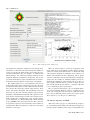
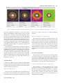
1
Aperture Photometry Tool
Author(s): Russ R. Laher, Varoujan Gorjian, Luisa M. Rebull, Frank J. Masci, John W. Fowler,
George Helou, Shrinivas R. Kulkarni and Nicholas M. Law
Reviewed work(s):
Source: Publications of the Astronomical Society of the Pacific, Vol. 124, No. 917 (July 2012),
pp. 737-763
Published by: The University of Chicago Press on behalf of the Astronomical Society of the Pacific
Stable URL: http://www.jstor.org/stable/10.1086/666883 .
Accessed: 09/08/2012 11:48
Your use of the JSTOR archive indicates your acceptance of the Terms & Conditions of Use, available at .
http://www.jstor.org/page/info/about/policies/terms.jsp
.
JSTOR is a not-for-profit service that helps scholars, researchers, and students discover, use, and build upon a wide range of
content in a trusted digital archive. We use information technology and tools to increase productivity and facilitate new forms
of scholarship. For more information about JSTOR, please contact [email protected].
.
The University of Chicago Press and Astronomical Society of the Pacific are collaborating with JSTOR to
digitize, preserve and extend access to Publications of the Astronomical Society of the Pacific.
http://www.jstor.org
PUBLICATIONS OF THE ASTRONOMICAL SOCIETY OF THE PACIFIC, 124:737–763, 2012 July
© 2012. The Astronomical Society of the Pacific. All rights reserved. Printed in U.S.A.
Aperture Photometry Tool
RUSS R. LAHER,1 VAROUJAN GORJIAN,2 LUISA M. REBULL,3 FRANK J. MASCI,4 JOHN W. FOWLER,4
GEORGE HELOU,4 SHRINIVAS R. KULKARNI,5 AND NICHOLAS M. LAW6
Received 2010 March 29; accepted 2012 May 24; published 2012 July 10
ABSTRACT. Aperture Photometry Tool (APT) is software for astronomers and students interested in manually
exploring the photometric qualities of astronomical images. It is a graphical user interface (GUI) designed to allow
the image data associated with aperture photometry calculations for point and extended sources to be visualized and,
therefore, more effectively analyzed. The finely tuned layout of the GUI, along with judicious use of color-coding
and alerting, is intended to give maximal user utility and convenience. Simply mouse-clicking on a source in the
displayed image will instantly draw a circular or elliptical aperture and sky annulus around the source and will
compute the source intensity and its uncertainty, along with several commonly used measures of the local sky
background and its variability. The results are displayed and can be optionally saved to an aperture-photometrytable file and plotted on graphs in various ways using functions available in the software. APT is geared toward
processing sources in a small number of images and is not suitable for bulk processing a large number of images,
unlike other aperture photometry packages (e.g., SExtractor). However, APT does have a convenient source-list tool
that enables calculations for a large number of detections in a given image. The source-list tool can be run either in
automatic mode to generate an aperture photometry table quickly or in manual mode to permit inspection and
adjustment of the calculation for each individual detection. APT displays a variety of useful graphs with just
the push of a button, including image histogram, x and y aperture slices, source scatter plot, sky scatter plot,
sky histogram, radial profile, curve of growth, and aperture-photometry-table scatter plots and histograms. APT
has many functions for customizing the calculations, including outlier rejection, pixel “picking” and “zapping,”
and a selection of source and sky models. The radial-profile-interpolation source model, which is accessed via
the radial-profile-plot panel, allows recovery of source intensity from pixels with missing data and can be especially
beneficial in crowded fields.
two-dimensional area used to define just the portion of a photograph or digital image of the nighttime sky that contains most, if
not nearly all, of the observed radiance of the astronomical object under investigation. Conventionally, the aperture is centered
on the source of interest, although the calculation is usually insensitive to exact aperture placement, and, in some cases, it is
desirable to offset the aperture slightly from the source’s center
to possibly omit the effect of a neighboring source. The shape of
the aperture is circular in its simplest form. Often, the shape of
an astronomical object, such as a spiral galaxy viewed at an oblique angle, will determine the aperture shape that is optimal for
its scientific study (e.g., elliptical). In addition to geometrical
considerations, photometric criteria can govern the aperture’s
shape (e.g., a set of contiguous pixels in a digital image with
data values greater than some threshold). A multiplier greater
than one, called an aperture correction, is employed to correct
for source intensity outside of the aperture, which is needed for
cases where source-crowding effects warrant using a smaller
aperture. In theory, an aperture correction is always needed
because of limited bandwidth considerations, but, in practice,
no aperture correction is made for sufficiently large apertures.
As the size of an aperture is increased, the signal from the source
1. INTRODUCTION
Aperture photometry in astronomical image-data analysis is
a basic technique for measuring the brightness of an astronomical object, such as a star or galaxy. It is the calculation of source
intensity by summing the measured counts from a subimage
containing the source (or possibly sources) and subtracting
the sky background contribution estimated from a nearby imaged region that excludes the source of interest (Da Costa
1992). The subimage containing the source brightness, or
so-called aperture, is a bounding region for the calculation, a
1
Spitzer Science Center, California Institute of Technology, Mail Stop 314-6,
Pasadena, CA 91125; [email protected].
2
Jet Propulsion Laboratory, California Institute of Technology, Mail Stop 169506, Pasadena, CA 91109.
3
Spitzer Science Center, California Institute of Technology, Mail Stop 220-6,
Pasadena, CA 91125.
4
Infrared Processing and Analysis Center, California Institute of Technology,
Mail Stop 100-22, Pasadena, CA 91125.
5
Caltech Optical Observatories, California Institute of Technology, Mail Stop
249-17, Pasadena, CA 91125.
6
Dunlap Institute for Astronomy and Astrophysics, University of Toronto,
Room 101, Toronto, ON Canada M5S 3H4.
737
738
LAHER ET AL.
becomes more fully contained and the noise encompassed by
the aperture is increased, and the signal-to-noise ratio (S/N)
of the aperture photometry result is therefore decreased; these
considerations mainly influence the size of the aperture chosen
for a study.
Aperture photometry calculations, as mentioned above, also
normally involve subtracting the contributions to the image data
that do not originate from the source of interest, which is generally referred to as the “sky background.” An annulus centered
on the source may define a region containing the image-data
pixels used to locally estimate the background, under the assumption that the background is constant across the aperture.
This assumption is violated to varying degrees in the case of
crowded fields, depending on the level of the crowding. The
annulus is commonly either circular or elliptical, and the annular
hole is as large as the aperture or larger, in order to exclude a
significant amount of signal from the source of interest for accurate sky background estimation. The inner and outer major
and minor radii of an elliptical annulus are the geometrical
parameters that determine the number of data samples involved
in the background estimation. The outer annular dimensions
should be small enough to keep the calculation local to the
source, but large enough to contain enough samples to sufficiently minimize the statistical uncertainty.
Aperture photometry, therefore, has its complexities. It is
often practical, more instructive, and sometimes more accurate
to perform aperture photometry manually on individual sources,
rather than to rely on results from automated software programs,
such as SExtractor (Bertin & Arnouts 1996; Holwerda 2005).
The intended audience for this article is anyone who is
interested in aperture photometry, including professional and
amateur astronomers and astronomy students. We introduce free
interactive software called Aperture Photometry Tool (APT)
that performs aperture photometry calculations and digitalimage analysis in a highly demonstrative manner. The software
is designed to be used with astronomical science images, which
are freely available from a variety of public data archives (e.g.,
the Spitzer Heritage Archive7). The software is thus suitable for
the classroom, but, not only that, it is also an effective analysis
tool for astronomical research. This article gives many details
about how to use the software and how it works. The objective
of the software is to make aperture photometry easy, more
accurate, and even fun, through an intuitive graphical user interface (GUI). The software enables aperture photometry to be performed interactively and gives visual feedback in various ways
to facilitate learning and calculational refinement. According to
Howell (1992), “We are all students in the astronomy game,”
and, in the context and spirit of that remark, APT was developed
to provide a better understanding of aperture photometry and its
computed results.
7
See http://sha.ipac.caltech.edu.
Our initial goal was to create a GUI-based aperture
photometry software application that is instructive on how to
perform aperture photometry, but, over time, the fruits of our
labor evolved into software that works well enough for professional use in research. APT has been used in the setting of involving teachers and students in original astronomical research
as part of the Spitzer Space Telescope Research Program for
Teachers and Students (Daou et al. 2005; Rebull et al. 2011)
and is now being used in that program’s successor, the
NASA-IPAC Archive Teacher Research Project (NITARP9).
Moreover, the research has led to new scientific discoveries
(Rebull et al. 2011). Generally, APT users report a positive experience with the software, and many find it easy to install on
their computers themselves.
The initial beta version of APT was released in 2007 November, and since that time, there have been many releases of the
package to add new capabilities and fix bugs.10
APT is an object-oriented, all-Java software implementation,
and, as such, the same source code is built to generate software
packages for Java-capable computers. Currently, four different
packages are available to facilitate installation on various types
of computers. There are no software dependencies on other astronomical packages or libraries. However, a recently installed
version of the Java Runtime Environment (JRE) is required.8
Version 2.1.5 of APT is available at the time of completion
of this writing, and it was compiled with JDK 1.6.0_31.
The structure of this article is as follows. Section 2 discusses
the design considerations that went into creating APT. Section 3
tours the layout of APT’s main GUI panel. Section 4 gives basic
APT usage instructions for users wanting a quick start. Section 5
explains how APT does sky background estimation and the
available options for controlling it. Section 6 provides details
on how APT does aperture photometry calculations and what
options are available for refining the calculations. Section 7 contains several subsections that discuss APT’s salient components,
functionality, applicability, and usage: image display, user preferences, output files, columns in the output aperture photometry
table, graphs, radial-profile interpolation, pick/zap tool, sourcelist processing, source-list generation, simple photometric calibration, image comparator and blink capability, batch mode, and
internationalization. Section 8 covers software limitations and
future upgrade plans. A summary is provided in the concluding
section.
9
See http://nitarp.ipac.caltech.edu.
APT can be downloaded from http://www.aperturephotometry.org. This
Web site has also has information on using APT, including installation instructions for Mac OS X, Linux, Windows, and Solaris machines.
8
APT requires the following packages: JFreeChart (www.jfree.org), JRegEx
(jregex.sourceforge.net), and Jama (math.nist.gov/javanumerics/jama), plus a
handful of the Spitzer Science Center Spot/Leopard Java classes for the astrometric calculations. These come packaged with APT, and so the user need not
install them separately.
10
2012 PASP, 124:737–763
APERTURE PHOTOMETRY TOOL
A companion article, in the same issue of the PASP that this
article appears, gives a quantitative comparison of calculational
results from SExtractor and APT with identical inputs, for the
case of noncrowded sources (Laher et al. 2012). The article
shows that both software programs give results that are generally in excellent agreement, especially for bright sources, and
seeks to find explanations for the discrepancies that occur for
faint sources.
Users who want to begin using APT right away may download and install the software, and then skip directly to the tutorial in §4.
2. DESIGN CONSIDERATIONS
APT is meant to complement, rather than supplant, prevailing noninteractive (batch-mode) aperture photometry software programs (e.g., the aforementioned SExtractor11). APT
was modeled after the popular DS9 FITS viewer (Joye and
Mandel 2003) in some ways, but with a focus on advanced aperture photometry capabilities. There are other interactive software programs that do aperture photometry, such as IRAF,12
which is a well-established workhorse in the astronomical community, but these can be difficult to install and less than straightforward to use, especially for nonspecialists. There are also
commercial aperture photometry software packages that are
popular with astronomers (e.g., the Interactive Data Language
and associated IDL Astronomy User’s Library13), which are
available at some cost. APT was designed to address these
points and also to have unique features and functions not found
in other aperture photometry programs.
Why is it desirable to visualize the data and interact with the
aperture photometry calculations? There are many answers to
this question, and the problems associated with aperture photometry are not easily realized until one looks at the data. For
example, an astronomer may not be aware that an astronomical
source of interest is in the “crust” of a mosaicked image, which
has a lower depth of coverage and ipso facto implications of
higher measurement uncertainty. Or, one may not realize that
a source has a significant number of blank or missing pixels
(i.e., pixels set to NaN [not a number] or Inf, [infinity]), even
though SExtractor may have yielded FLAGS=0 for that source.
The accuracy of the background estimation can have a substantial effect on the results, especially for large apertures and relatively faint sources. In many cases, one will want to look at the
contents of the image region used for background estimation as
a sanity-check and possibly make adjustments.
With the above considerations in mind, the classroomsuitability criteria that we adopted for APT are listed as follows:
11
See http://www.astromatic.net/software/sextractor.
IRAF stands for Image Reduction and Analysis Facility; see http://iraf.noao
.edu and Tody (1986, 1993).
13
See http://idlastro.gsfc.nasa.gov.
12
2012 PASP, 124:737–763
739
visualization of inputs and outputs, user interaction, ease of use,
ability to run on a variety of machines and operating systems,
ease of installation, and zero acquisition cost.
Data visualization pertains to graphical and statistical representations of not only the aperture photometry results, but also
the input data. We found that showing an overlay of the aperture
and sky annulus on the input image was important in giving the
user important visual information for setting up the aperture
photometry calculation in relation to the astronomical source
of interest and its environs. APT’s GUI has many controls that
promote user interaction, such as changing the size of the aperture and sky annulus, and then immediately seeing the resulting
overlay. The feedback provided by APT’s various graphs allows
the user to make intelligent choices in modifying the input
parameters. The overall effect of equipping APT with a rich
palette of controls and capabilities is to engage the user, so that
the user will want to spend time running the software. At least,
this is our aim.
It is important to us that the software is able to be executed on
a variety of machines, particularly Mac, Windows, and Linux
computers, which are the most popular today. It is for this reason
that we chose to implement APT in the Java programming language. In fact, any computing platform that runs the Java Virtual
Machine (JVM) can run APT. We also programmed APT with
special functionality to enable it to run on computers with smaller
memories and with smaller screens. APT’s minimum memory
requirement is, by design, very modest, only around 300 Mbytes
with a 2048 × 4096-pixel image loaded. This is small enough to
accommodate older machines often found in the classroom.
APT can be easily used on machines with relatively small memories to analyze portions of very large images. This is effected by
configuring APT’s maximum image size to as little as 500 pixels
on a side. APT can also be set up with a compact-sized GUI that
fits on some computer screens that are smaller than normal in
size, such as those on the smaller laptops.
APT has relatively simple installation instructions (some
APT users have reported that APT is much easier to install than
IRAF). We have eliminated all high-level software dependencies by putting it in a single package to simplify the process.
Additionally, we have refined the installation process down
to just a handful of steps. APT is especially easy to install on
a Mac.
Finally, the software can be downloaded via the Internet and
used free of charge for research and education in astronomy and
astrophysics, satisfying the last criterion in our list of classroomsuitability attributes.
3. MAIN GUI PANEL
This section summarizes the prominent features of APT’s
main GUI panel, with more details given later in §7. The layout
of APT’s main GUI panel is shown in Figure 1, and the
enumeration below in this section refers to the numbered items
in the figure. The computer screen shots in Figure 1 and other
740
LAHER ET AL.
FIG. 1.—APT’s main GUI panel. The numbers with arrows highlight the components that are described in § 3.
figures shown in this article were taken on an Apple
computer running OS X Lion and will have slightly different
appearances under other operating systems. When running the
software, hovering the mouse cursor over a widget in the GUI
will cause a short pop-up explanatory note or tool tip to be
displayed.
Not shown in Figure 1 are the Preferences, File, and Tools
pull-down menus, which are located at the top of the computer
screen in the case of Macs, or in the main GUI panel’s upper-left
corner in the case of non-Mac machines. Section 7.2 gives more
information about the Preferences menu. Currently, the File
menu only has one option, which is to clear the contents of
the output aperture-photometry-table file. Section 7.10 discusses the tool-menu option of performing simple photometric
calibration of astronomical sources extracted from an image.
The remainder of this section gives descriptions for the numbered items called out in Figure 1:
1. The Get Image button is used to load an image and display
it in the GUI. The actions associated with this button have functionality to load either a primary image or a comparator image.
The primary image is, by definition, the first image loaded, and
the subsequently loaded images are called comparator images,
whose purpose is visual comparison with the primary image
(see § 7.11). Up to three comparator images are permitted.
Aperture photometry calculations are done only for the primary
image. APT can read only FITS-formatted images.14 This
includes single-extension FITS files, FITS files with multiple
image-data planes in a single image extension, and FITS files
with multiple image extensions (but not those with binary-table
extensions).
2. The FITS header button pops up a panel that lists the FITS
header of the primary image. In the case of a multiextension
FITS file, the headers of all extensions are listed. The top of
the panel has functionality for case-sensitive searches, which
is useful for finding particular keywords, values, and comments
in the FITS-header listing.
3. The pull-down menu with the default label 1%=99% has
several options for setting the limits of the image-display
stretch, which is the mapping of pixel intensities to values in
the 0–255 range for 8-bit graphics. The options include the
image-data minimum and maximum, as well as various combinations of image-data percentiles. As the default label indicates,
the default setting for stretch is the selection with the 1 and 99
percentiles. Located above this pull-down menu on the main
GUI panel are text fields that display the lower and upper
bounds of the stretch corresponding to the menu selection made
(see item 34 below).
14
FITS stands for Flexible Image Transport System; see http://fits.gsfc.nasa
.gov and Wells et al. (1981).
2012 PASP, 124:737–763
APERTURE PHOTOMETRY TOOL
4. The Source List button pops up a panel for performing a
large number of aperture photometry calculations at source
positions that are read from a source list (see § 7.8). From this
panel, additional functionality for generating a source list automatically is available (see § 7.9).
5. The Image Histogram button pops up a panel with a histogram plot for the entire primary image (see Fig. 2). The lower
and upper limits of the graph’s horizontal axis are set by the
image-display stretch bounds. This histogram is, of course, useful for determining the best stretch. There is an inset table of
global-image-data statistics on the graph: minimum, maximum,
mean, sigma (standard deviation), median, scale (a robust measure of the data dispersion, given by one-half the difference
between the 84.1 and 15.9 percentiles, which is equivalent to
1 standard deviation in the case of Gaussian-distributed data),
1 and 99 percentiles, number of data values used in computing
the statistics, and number of pixels set to either NaN or Inf in the
image data. The intent of the displayed statistics is to make the
user aware of the image-data contents. Except for the number
counts, the data units of the image statistics are given by the
image’s BUNIT FITS-header keyword, or, if BUNIT is not
available, the default is D.N. (digital or data number). The
default setting can be changed via the Set Default Image-Data
Units option in the Preferences menu.
6. The About & Help button pops up a panel showing the
software version number and the built-in documentation.
7. The Exit button terminates the software program in a
user-friendly way (one more chance is given to cancel the
termination).
8. The Image Comparator button pops up a panel displaying
the primary image on the left side of the panel and up to three
comparator images on the right for a side-by-side comparison
(see § 7.11).
9. The main image-viewing panel displays either the primary
image or a comparator image (see item 16 below). If the image
is bigger than the viewing window, then the scroll bars on the
window can be used to view the desired image portion (the user
may have to mouse-click on the image to make the scroll bars
appear). Bounding-box graphics are overlaid onto the image
just outside the visible portion of the image, in order to visually
define the region updated by the Refresh 1 button (see item 14
below). The example image in Figure 1 is a Spitzer Space Telescope mosaic, with pixels having missing data represented by
the blank color blue. The left-middle side of the image containing data has an aperture and sky annulus overlay, which is
drawn by the software when the user mouse-clicks on a source
in the displayed image.
10. The filename label indicates the image currently displayed in the main image-viewing panel (see previous item).
The label is embedded with additional useful information.
The number enclosed in the first set of square brackets indicates
whether the currently displayed image is the primary image
(value is 1) or a comparator image (value is greater than 1). The
two numbers separated by a colon and enclosed within the second set of square brackets indicate the image-extension number
and the image-data-plane number within the image extension,
respectively.
11. The image-display graphic shows the currently selected
display type and color table. The available types are grayscale,
inverted grayscale, false color, and inverted false color. There
are two false-color tables available: one is called contour because it seeks to differentiate adjacent colors in the color table,
FIG. 2.—Sample image-histogram plot generated by APT.
2012 PASP, 124:737–763
741
742
LAHER ET AL.
and the other (eponymous) color table has a gradation of rainbow colors. There are 24 levels of grayscale or 24 hues in the
color tables. The display type and color table can be set via options in the Preferences menu. See item 28 below for related
information on the Color-Table Toggle button.
12. The image-magnifier panel displays a subimage of the
image currently shown in the main image-viewing panel. The
subimage is centered at the mouse-cursor position in the main
image-viewing panel. The subimage is changed in real time as the
mouse cursor is moved. The magnification options of the imagemagnifier panel are 5×, 10× (the default setting), and 20×.
13. The Refresh 2 button repaints the image for both visible
and nonvisible portions of the image in the main image-viewing
panel. This is useful after image-display characteristics, such as
the stretch or color table, have been changed. After the short
amount of time required for this operation to complete, the main
image-viewing panel’s scroll bars can be used to quickly scroll
about the entire image, which will be thereafter displayed with
the same image-viewing characteristics (until such time that
image-viewing changes are made again).
14. The Refresh 1 button repaints the visible portion of the
image in the main image-viewing panel, plus the relatively small
nonvisible portion that lies within the bounding-box graphics
(see item 9). This option is faster than the repainting of the entire
image done by the Refresh 2 button and is mainly useful for redrawing the bounding-box graphics and eliminating any residual
bounding-box graphics in the visible portion of the displayed
image. The latter can occur after the scroll-bar positions of the
main image-viewing panel have been moved or after the main
GUI panel has been enlarged. For the most part, the visible
portion of the image is repainted automatically after changes to
image-viewing characteristics, such as the stretch or color table.
15. The Pick/Zap button pops up a panel with the pick/zap
tool (see §7.7).
16. The Blink button is for image blinking the primary image
and up to three comparator images (see § 7.11).
17. The Thumbnail button pops up a panel that is capable of
displaying the entire primary image, rather than just the portion
of it that may be currently displayed in the main image-viewing
panel. At the top of the thumbnail panel are a Show Grid button
and a display of real-time mouse-cursor position in both image
and equatorial coordinates, as well as a display of the real-time
pixel-data value at the cursor position. The Show Grid button
will overlay a grid labeled with equatorial coordinates and then
subsequently transform into a Hide Grid button. If a world
coordinate system (WCS) is not available in the image’s FITS
header, then the grid overlay will be disabled. The thumbnail
image can be made to fit on the user’s computer screen using
the Set Maximum Thumbnail Size option in the Preferences
menu. If it is set to larger than the user’s screen, then the panel
will be automatically scaled to fit and scroll bars will appear.
Figure 3 shows an example primary-image thumbnail with a
coordinates-grid overlay.
18. The Recompute Photometry button repeats the aperture
photometry calculation after changes to its setup have been
made, such as different aperture geometrical parameters. Such
changes, which affect the results, cause the Recompute Photometry button text to change from the color black to the color
red as a reminder to the user that the calculation needs to be
updated. More details about how this button works and is used
are given in §§ 4, 6, 7.7, and 7.8.
19. The Plot Results button pops up a panel that allows the
setting up of scatter plots of one data column in the output aperture photometry table versus another. Histograms of data columns can also be plotted. Section 7.5 describes the available
functionality in more detail.
20. The List Results button pops up a spreadsheet-style listing of the output aperture photometry table. The data columns in
the table are fully described in § 7.4.
21. The Save Results button stores a record of the latest aperture photometry calculation as a single row in the output
aperture-photometry-table file. A calculation may be manually
repeated many times with different settings, but it is not saved in
the file until this button is utilized, and then only the last result
is saved.
22. The More Settings button pops up panel that enables
parametric changes to the aperture photometry calculation, including the specification of source and sky models. The options
and controls on this panel are fundamental to utilizing APT to
its fullest and are described in §§ 4, 5, and 6, as well as
mentioned throughout the remainder of this article.
23. The main results of the latest aperture photometry calculation are displayed near the lower-left corner of the main GUI
panel, under the heading PRIMARY-IMAGE PHOTOMETRY
RESULTS. Section 7.4 defines the displayed quantities, which
are among the quantities written to the output aperture photometry table when the user mouse-clicks on the Save Results
button.
24. The Snap button nudges the aperture onto the computed
centroid of the source of interest (see § 6 for more details, including the color-coding).
25. The source’s centroid position, in floating-point pixels, is
displayed just to the left of the Snap button (see § 6).
26. The aperture’s position, in integer pixels, is displayed in
spinner-controllable text fields and can be changed here via either text-field editing or mouse-clicking on the tiny increment/
decrement buttons located just to the right of the corresponding
text field.
27. The real-time pixel coordinates, the corresponding equatorial coordinates, and the image-data value at the position of the
mouse cursor in the main image-viewing window are displayed
under the heading REAL-TIME RESULTS. The representation
of the sky coordinates can be changed to either sexagesimal or
decimal degrees via theSet Celestial-Coordinates Units option
in the Preferences menu. The image-data units are given alongside the image-data value. The default image-data units are used
2012 PASP, 124:737–763
APERTURE PHOTOMETRY TOOL
FIG. 3.—APT’s primary-image thumbnail.
2012 PASP, 124:737–763
743
744
LAHER ET AL.
when the BUNIT keyword is absent from the image’s FITS
header and can be set via the Set Default Image-Data Units option in the Preferences menu.
28. The six buttons on the left of the button group, Aperture
Slice, Curve of Growth, Source Scatter, Radial Profile, Sky
Scatter, and Sky Histogram, pop up various graphs associated
with the current calculation (see § 7.5). On the right, the Hide
Aperture button temporarily hides the aperture overlay and subsequently transforms into the Show Aperture button and the
Color-Table Toggle button that successively switches to the
available presequenced color-table options (see item 11 above).
29. The Alter button next to the aperture-attributes label pops
up a panel that allows changes to the elliptical aperture’s major
and minor radii and rotation angle (see Fig. 4), and the button’s
label indicates the values of these parameters. The text fields in
the group allow changes to values of the centroid, inner-sky, and
outer-sky major radii, in integer pixels. The default aperture
shape is circular, in fact, and the default settings for the centroid,
aperture, inner-sky, and outer-sky radii are 5, 5, 8, and 15 pixels,
respectively. These defaults can be changed via the Preferences menu.
30. The Stretch-Type Toggle button cycles the image-display
stretch from linear to logarithmic to histogram equalization and
then back to linear.
31. The dynamic range slide control allows the dynamic
range of the logarithmic image-display stretch to vary from 0
FIG. 4.—APT’s panel for setting the elliptical-aperture attributes.
(equivalent to a linear stretch) to 5 orders of magnitude (which
visually differentiates the smallest image-data values that are
above the lower bound of the stretch). The default setting is
one order of magnitude. The slide control is disabled for nonlogarithmic types of stretches.
32. The stretch minimum and stretch maximum slide controls allow the lower and upper limits of the image-display
stretch, respectively, to be varied from their current settings.
The new stretch is instantiated only after the Stretch to Bounds
button is pressed (see next item).
33. The Stretch to Bounds button sets the limits of the imagedisplay stretch to the two values in the lower-bound and upperbound text fields (see next item).
34. The lower and upper limits of the current image-display
stretch can be manually changed by typing new values into the
lower-bound and upper-bound text fields, respectively. The user
must either press Enter on the keyboard or mouse-click on the
Stretch to Bounds to apply changes made directly to these text
fields.
4. BASIC USAGE INSTRUCTIONS
APT is intended to be simple to use. Basically, one displays a
FITS image and then mouse-clicks on a source (i.e., an astronomical object) shown in the main image-viewing panel to overlay an elliptical aperture onto it. The latter action causes the
software to automatically perform an aperture photometry calculation. The computed quantities include, among others,
source centroid position, source intensity, source-intensity uncertainty, sky background level, and sky background dispersion
width. The default sky algorithm is no sky background subtraction from the source intensity, and the reason for this is
to facilitate proper use of APT’s radial-profile interpolation
capability. More often than not, however, the user will require
the sky background to be subtracted from the source intensity, in
which case this sky model can be selected from the control panel
that pops up after mouse-clicking on the More Settings button
(located in the lower-left corner of the main GUI panel; see
also item 22 in § 3). See Figure 5 for a depiction of the More
Settings panel.
The general flow of the work progresses from the buttons and
controls in the upper-left region of the main GUI panel to the
middle-left region and then lower-left region of the same. Here
are the basic instructions.
1. Take a moment to review the default settings by selecting
List Preferences from the Preferences menu. More information on user preferences and how to change them is given
in § 7.2.
2. Choose a primary image to display by mouse-clicking on
the Get Image button in the upper-left corner of the GUI panel.
The primary image, as defined here, is the first image displayed
in the main image-viewing panel (after the primary image is
loaded, a subsequent mouse-click on the Get Image button will
2012 PASP, 124:737–763
APERTURE PHOTOMETRY TOOL
745
FIG. 5.—APT’s More Settings panel.
allow the user to load either a different primary image or comparator images).
3. Adjust the image-display stretch for best viewing. As an
aid, click on the Image Histogram button to see the stretch range
spanned by the image.
4. Select centroid and sky annulus major radii (integer values
only), and click on the Alter button beside the aperture-attributes
label to select the elliptical aperture attributes, as appropriate for
the source of interest.
5. Place the mouse cursor over the source of interest in the
image displayed in the main image-viewing panel and click to
overlay an aperture.
6. Show and study the various graphs (instructions are given
in § 7.5).
7. Select the desired new radii, as appropriate, and/or change
other settings as needed.
2012 PASP, 124:737–763
8. Redraw or overlay a new aperture by either clicking
on the Recompute Photometry button or clicking on the
Snap button for nudging the aperture onto the source centroid location or placing the mouse cursor on the image and
clicking.
9. If necessary, increment or decrement the spinner controls
for fine-tuning the aperture’s position.
10. Click on the Recompute Photometry button to redraw/
overlay a new aperture.
11. Show and study the various graphs again.
12. Optionally click on the Save Results button, located in
the lower-left corner of the main GUI panel, in order to save/
append the results to APT’s output photometry-table file (e.g.,
APT.tbl). The adjacent List Results and Plot Results buttons can
be used to list and plot the saved results.
13. Repeat the above steps for each source of interest.
746
LAHER ET AL.
5. SKY BACKGROUND ESTIMATION
Strictly speaking, the background should be the best estimate
of the true underlying background emission, excluding contamination from the source flux being measured, and not biased by
any other neighboring sources or outliers. As a practical matter,
we estimate the background in the aperture from an elliptical
sky annulus surrounding it, and this method does not account
for gradients in the sky background caused by sources in the
annulus. A bright source in the sky annulus contributes to
the background in the aperture, and its effect is not necessarily
something that is to be completely ignored or filtered out, which
is why APT has a variety of sky models from which to choose.
APT has fairly straightforward methods for estimating the
sky background in the region local to the source of interest,
and there are a few options available for controlling how it
is done. Only image pixels in an elliptical sky annulus centered
on a user-selected center position are considered for the background calculation. The pixels with NaN or Inf are rejected
outright. The center position, for purposes of background estimation, is specified in integer pixels only. There are three different ways of specifying the center position in APT:
1. Mouse-clicking on the image displayed in the main imageviewing panel.
2. Changing the values in the spinner-controllable text fields
for the aperture position, which are located near the lower-left
corner of the main GUI panel.
3. Clicking on the Snap button in the lower-left corner of the
main GUI panel (more on this in § 6).
The inner and outer major radii of the sky annulus, in integer
pixels only, can be specified on the main GUI panel. These
major radii are used to scale the ellipse specified for the aperture. The inner radius of the sky annulus must be greater than or
equal to the radius of the elliptical aperture along any direction
from the center of the ellipse. No limitation is placed on the
outer radius of the sky annulus, except that it must be greater
than the inner radius. The default values that specify the size and
shape of the aperture and sky annulus, which are loaded when
APT is launched, can be specified via the Set Photometry Size
Parameters option under the Preferences menu.
On the APT control panel that pops up after clicking on the
More Settings button, the user can select from one of four available sky models:
Model A.—No sky background subtraction.
Model B.—Sky median subtraction.
Model C.—Custom sky subtraction.
Model D.—Sky average subtraction.
Sky median subtraction is less sensitive than sky average
subtraction to other bright sources that may fall within the sky
annulus, which might otherwise cause the background to be
overestimated. If model C is specified, then the custom value
to be used must be specified in the text field labeled Custom
sky value on the More Settings panel.
The More Settings panel has text fields where the user can
optionally specify lower and upper thresholds for the rejection
of outlier pixels in the sky annulus from the background calculation. The default values for the lower and upper thresholds are
the largest possible negative and positive double-precision numbers, respectively, so that, by default, no pixels are rejected. The
values for the outlier-rejection thresholds must be given in the
data units of the image’s FITS file. It is best to study the various
aperture photometry graphs provided by APT, in order to figure
out the best thresholds, and then set these thresholds before
optionally converting the image-data units into the desired
source-intensity units (see § 7.5 for how to do the latter).
In addition to the aforementioned outlier rejection, there is
yet another outlier-rejection method that is applied. The median
and standard deviation are computed, and all data values that lie
greater than 3 standard deviations from the median are rejected.
Currently, this number of standard deviations is hard-coded and
cannot be changed by the user.
The pixel zap functionality of the pick/zap tool can also be
used to temporarily eliminate pixels from the background calculation. More details about the pick/zap tool are given in § 7.7.
The median and average of the remaining image data in the
sky annulus after the outlier rejection have been applied are
computed as possible background estimators. The median or
average times the number of pixels in the aperture form a product that is the sky contribution optionally subtracted from the
integrated image data of the source to get the backgroundsubtracted source intensity. These quantities are labeled Sky_
median/pix and Sky_average/pix, respectively, in the output
aperture photometry table (see § 7.4). The standard deviation
is computed for the Sky_sigma column in the aperture photometry table. Likewise, the root-mean-squared (rms) value is computed for the Sky_RMS/pix column. The Sky_scale column, a
robust estimator of the data dispersion, is computed as one-half
of the difference between the 84 and 16 data percentiles.
6. APERTURE PHOTOMETRY IMPLEMENTATION
The aperture photometry calculation primarily yields the
source intensity and its uncertainty. The former involves summing pixel values within the aperture to get the total intensity,
then subtracting the product of the aperture area, in pixels2 , and
the per-pixel sky background, in order to get the source intensity. The latter also requires the aperture and sky annulus geometry, as well as extra information, including the detector gain,
the conversion factor from image-data units to D.N. (if image
is not already in units of D.N.), the background-estimation
method, and the sky background standard deviation. APT works
under the assumption that the background is constant across the
aperture.
APT performs its calculations with an elliptical aperture,
which the user specifies with major and minor radii and a rotation angle. These quantities are recorded in the MajR_aper,
MinR_aper, and Rot_aper columns, respectively, in the output
2012 PASP, 124:737–763
APERTURE PHOTOMETRY TOOL
aperture photometry table (see § 7.4). Of course, APT also
allows circular apertures, as a circle is a special case of an ellipse
with its major radius equal to its minor radius.
The basic inputs for the calculation are the elliptical-aperture
geometrical parameters, the source centroid major radius, and
position coordinates of the aperture center (the instructions
for selecting these quantities are given in § 5). The calculation
of the source’s centroid position, which shares the same center
position as the aperture, can involve a different number of pixels
than used in the calculation. The source centroid ellipse is its
major radius scaled to the ellipse specified for the aperture.
The aperture geometrical parameters and centroid major radius
can be specified on the main GUI panel.
The More Settings panel has text fields where the user can
optionally specify lower and upper thresholds for rejection of
spurious aperture pixels in the calculation. The default values
for the lower and upper thresholds are the largest possible
negative and positive double-precision numbers, respectively,
so that, by default, no pixels are rejected. Again, values for
outlier-rejection thresholds must be given in image-data units.
The pixel zap functionality of the pick/zap tool can also be
used to temporarily eliminate pixels from the calculation. More
details about the pick/zap tool are given in § 7.7.
The method that computes the source centroid position is
iterative and runs for 100 iterations. The first iteration is bootstrapped from the user-selected aperture position. The k þ 1th
iteration computes the following x and y image coordinates of
the source centroid:
P
kþ1
¼ xkcentroid þ
xcentroid
ðxi xkcentroid Þðdij dkmin Þ
i;j∈SðkÞ
P
ðdij dkmin Þ
;
(1)
;
(2)
i;j∈SðkÞ
and
P
kþ1
¼ ykcentroid þ
ycentroid
i;j∈SðkÞ
ðyj ykcentroid Þðdij dkmin Þ
P
ðdij dkmin Þ
i;j∈SðkÞ
where the sums are over pixels in the centroid ellipse SðkÞ that
meet criteria given below; image data value dij is located at pixel (xi , yj ); and dkmin is the smallest data value in the centroid
ellipse. The data values included in the summing must be greater than dkmin , not NaN or Inf, and less than or equal to the upper
outlier-rejection threshold for the calculation. The centroid
ellipse is allowed to move with each iteration, so it is necessary
to recompute dkmin each time. The centroid calculation is done
with subpixel resolution, but the step size is currently limited to
no less than 0.05 pixels for computational speed. The method
generally converges for isolated sources, but not always, and the
user is cautioned to check that the resulting source centroid is a
reasonable one. The source centroid calculation does not always
2012 PASP, 124:737–763
747
give the best aperture position for the source of interest, especially if there are other sources nearby that fall within the
centroid ellipse. One can use visual feedback from the aperture-slice and source-scatter graphs for improved manual aperture positioning. See § 7.5 for more information about the
available APT graphs.
The More Settings panel has radio buttons for the user to
select one of three available source models:
Model 0.—No aperture interpolation.
Model 1.—Aperture interpolation only for NaN and Inf pixels (including zapped pixels).
Model 2.—Interpolation for all aperture pixels.
Model 0 will underestimate the source intensity if there are a
significant number of blank pixels in the aperture. Model 1 was
designed to remedy this, but it requires that the user set up a
radial-profile model for the interpolation, and APT has a tool
that makes it easy (as discussed in § 7.6). Model 2 uses the
radial-profile model to compute data values for all pixels in the
aperture and generally gives a result that is within a few percent
or better of model 0 if the radial-profile model was set up on the
same source. Model 2 is most useful in cases where the source
of interest has missing aperture pixels and the radial-profile
model was set up on a different source that has no missing pixels, which is facilitated by the built-in automatic scaling and
offsetting of the radial profile.
The aperture photometry calculation is done with subpixel
resolution. The default subpixel size is 0.01 pixels. The small
value can cause the computations to take several seconds for
very large aperture ellipses. The subpixel size can be changed
via the Set Calculation Step Size option in the Preferences menu.
By default, the calculation is performed with the aperture
centered on the calculated source centroid. The Centroid
ðX; Y Þ ¼ label on the lower-left side of the main GUI panel
is displayed in the color green to indicate that centroiding is
enabled and in the color black to indicate that it is disabled.
Unchecking the Use centroid in photometry calculation? check
box on the More Settings panel will do the disabling and cause
the calculation to revert to centering the aperture on the integer
pixel coordinates of the selected aperture position. Note that
although centroiding moves the center position of the aperture
with subpixel resolution, the center position of the sky annulus
is incremented only with integer-pixel resolution.
The Snap button in the lower-left main GUI panel is available
to nudge the aperture onto the computed source centroid location. After moving the aperture, it automatically recomputes the
photometric results (just like the Recompute Photometry button). If centroiding is turned on and the aperture is already fairly
close to the centroid, the recomputation may give the same non–
background-subtracted source intensity as before (with slight
changes possible to the source-intensity uncertainty, sky background, and sky background dispersion), and the main difference will be that the aperture will appear to be better
centered on the centroid position (and the data points plotted
748
LAHER ET AL.
in most of the APT graphs will be shifted accordingly). If centroiding is turned off, the user will obtain a new result at the new
aperture position, which, after snapping the aperture, will be
the centroid position represented by integer image coordinates.
The Snap button text will turn the color yellow to remind the
user to mouse-click on this button to fully center the aperture on
the centroid location. This color reminder can and should be
ignored if the user wants photometric results for an aperture that
is dislocated from the centroid position, in which case centroiding should be turned off.
The source-intensity-uncertainty calculation requires the
detector gain (electrons per D.N.), the conversion factor from
image-data units to D.N., and the depth of coverage. The default
value for these quantities is 1.0. When a primary image is
loaded, the software attempts to read the GAIN FITS keyword
and, if found, automatically overrides the default gain value. For
image data that are already in units of D.N., the value of 1.0 is
appropriate for the image-data-units-to-D.N. conversion factor.
A depth of coverage of 1.0 is correct for a single observation.
These quantities can be subsequently overridden on the More
Settings panel, after an image has been loaded. The default gain
value, used in the absence of the GAIN FITS keyword, can be
changed via the Set Default Image-Data Gain option in the Preferences menu.
APT computes the source-intensity uncertainty, σsrc , using
σsrc
sffiffiffiffiffiffiffiffiffiffiffiffiffiffiffiffiffiffiffiffiffiffiffiffiffiffiffiffiffiffiffiffiffiffiffiffiffiffiffiffiffiffiffiffiffiffiffiffiffiffiffiffiffiffiffiffiffiffiffiffiffiffiffiffiffiffiffiffiffi
κðAsrc σsky Þ2
F src
¼
þ Asrc σ2sky þ
;
ηGN depth
Asky
(3)
where F src is the sky-background-subtracted source flux density
or source intensity, G is the detector gain, N depth is the depth of
coverage, η is the conversion factor from image-data units to
D.N., Asrc is the aperture area (in pixels2 ), σsky is the sky background standard deviation (per pixel), κ is a factor that depends
on the optional background-estimation type or sky model employed in the computation (see below), and Asky is the area of
the sky annulus (in pixels2 ). Equation (3) has three terms under
the square-root sign. The first two terms are well known: e.g.,
see Bertin (2006b). The third term accounts for the uncertainty
in the background estimation, which SExtractor omits. Equation (3) does not account for possible pixel-to-pixel noise correlations, which are present in co-added images. The derivation
of this formula is beyond the scope of this article and may be
found in Masci and Laher (2012, in preparation).
Equation (3) allows that the image the user has in hand is not
necessarily as observed with the detector’s gain factor, but rather
the combination of some number of images, as in a co-added
image or mosaic. The depth of coverage can vary with source
position, and so this must be adjusted for each individual source.
The depth of coverage N depth can be specified on the More
Settings panel.
Depending on whether the APT-optional sky average, sky
median, or custom sky value is used in the sky background sub-
traction, the value of κ in equation (3) is equal to either 1.0, π=2,
or 0.0, respectively. In the first two cases, APT uses the sky
scale, which is defined in § 7.4, as a robust estimator of the
sky background standard deviation, σsky ; in the latter case,
σsky is taken to be zero. (In this article, robust refers to methods
that are generally somewhat less optimal than methods applicable to well-characterized noise, but more stable against
outliers. For example, the sample median is a robust estimate
of the population mean when the sample is contaminated,
but the sample mean is most optimal when the noise is wellbehaved.) In the artificial case of no sky background subtraction (an APT option that is useful in radial-profile interpolation,
as discussed in § 7.6), only the first term under the squareroot sign in equation (3) determines the source-intensity uncertainty.
The More Settings panel allows the user to specify two additional quantities related to the calculation. It provides for setting an aperture correction, a multiplicative factor greater than
1.0 that, when multiplied by the result for source intensity, accounts for the missing source intensity that becomes a problem
when the aperture is too small for the source. This is useful
when it is impractical to make the aperture as large as is needed,
such as in dense fields. The user can also set a magnitude zero
point, so that photometrically calibrated source magnitudes will
be computed. The magnitude zero point, if available for the image at hand, comes from prior photometric calibration against
reference stars either in the same image or in images acquired by
the telescope in the same night (and for the same camera filter
used). When the magnitude zero point is determined, it can
either be done for the image’s exposure time or normalized
to an image with a 1 s exposure time. The case that applies
should be documented and, therefore, known. If the latter is
the case, then the magnitude zero point for a 1 s exposure must
be corrected for the image’s exposure time before inputting to
APT, in order to yield accurate results, as APT does not do this
automatically. This correction is done by adding 2:5 log10 ðT exp Þ
to the time-normalized magnitude zero point, where T exp is the
exposure time, in seconds.
In the event adjustments are made to the GUI controls that
affect any of APT’s calculational results, the Recompute Photometry button text will change from the color black to the color
red as a reminder to the user that the calculation needs to be
updated. This visual device aims to reduce user errors resulting
from incorrect associations made between mutually inconsistent
inputs and outputs.
BUNIT is a keyword defined by the FITS standard for specifying the physical units of the image data. If this keyword is
missing or its setting is null in the image FITS header, then, for
clarity in various GUI-panel labels, the software will assume the
setting of the default image-data units. This can be changed via
the Set Default Image-Data Units option in the Preferences
menu, and it is initially D.N.
2012 PASP, 124:737–763
APERTURE PHOTOMETRY TOOL
749
7. SUPPLEMENTARY SOFTWARE FUNCTIONALITY
7.2. User Preferences
7.1. Image-Data Display
Various options in the Preferences menu allow users to
change the default settings and then save them to disk for a later
APT session. When APT is launched, it automatically loads the
preferences from a special file called APT.pref that is located in
the invisible subdirectory called .AperturePhotometryTool in
the user’s home directory.15 Users also have the option of later
manually loading in another preferences file from a different
disk location and filename. If the special preferences file does
not exist, then factory-default preferences are loaded into the
user’s session, but are not automatically saved—the user must
explicitly save them via the Save Preferences option in the Preferences menu, if that is what the user wants to do. Within a
given APT session, whenever a new primary image is read
in, the preferences are restored from the special preferences file.
Selecting the Reset Default Preferences option in the Preferences menu will restore the factory-default settings to the user’s
session, but will not save them (again, the user must manually
select the option to do this). If the Save Preferences option is
selected, then the current settings of the user’s session will
be written to a user-selected location and filename, and if that
file already exists, then all prior custom settings in that file will
be overwritten.
At any time during a user’s session, most of the current
settings, as set by the various GUI controls within and without
the Preferences menu, are the instantaneous user’s preferences
for the session (albeit not necessarily saved to disk). This can be
verified by mouse-clicking on the List Preferences function under the Preferences Menu. One exception is the setting of the
aperture geometrical parameters and the centroid and sky annulus inner and outer major radii, whose preferred values should
be set via the Set Aperture Size, Shape, and Angle and Set
Photometry Size Parameters options in the Preferences menu
(these values may be changed to other values directly on the
main GUI panel, as needed for experimentation, without affecting the preferences). Therefore, the Save Preferences option
will, for the most part, capture the current state of the user’s
session.
In the main image-viewing panel, which is located in the
upper-right corner of the main GUI panel, the stretch and colortable controls work automatically only for the visible portion of
the displayed image, plus some margin around the visible
image’s edges. This design feature allows the software to run
faster and be more responsive. The positions of the panel’s
scroll bars determine which portion of the image is visible
and actively updated when the image-viewing settings are
changed. Moving the scroll bars for large images will reveal
the once-active portion of the image inside a visually obvious
bounding box. The image outside of the bounding box will be
displayed with a different stretch and/or color table, which was
set earlier in the APT session. To remove the unsightly remnants
of the bounding box and refresh the displayed image, two refresh options are available. The Refresh 1 button quickly refreshes just the visible portion of the image to save time.
The Refresh 2 button refreshes the entire image by launching
multiple processor threads for refreshing the unseen portion
of the image, so that immediate GUI control is returned to
the user, and additional computer CPU cores, if available on
the user’s machine, are utilized to finish the job faster. For very
large images, however, the threads take some time to complete
and may still be running even though the user is allowed to continue normal work with the GUI. To avoid queueing up too
many threads, the user is advised to not mouse-click on the Refresh 2 button more than once in a reasonable time interval: at
least a few seconds. When needed, the Refresh 2 button text will
change from the color black to the color yellow to remind the
user to click on this button before scrolling about the image. It is
not mandatory for the user to click on the Refresh 2 button when
its text turns yellow; the user can defer doing this until after the
scroll bars are subsequently moved.
For purposes of image display only, all image-data values
outside the interval specified by the stretch extrema are set
to the corresponding extreme value. Image-data values that
are set to NaN or Inf are displayed with the blank color set
by the user (the color blue is the default). Inf values are handled
the same as NaN values, and almost no distinction is made between these two bad-data types. The blank color can be changed
using the blank color-picker accessible via the Set ImageDisplay Attributes option in the Preferences menu.
The user can specify the maximum image size that the software will load into memory. This is done using the Set
Maximum Image Size option in the Preferences menu. The default maximum image size is 5000 pixels on an image side, and
this preference can be reset to as many as 100,000 pixels. For
images larger than the preferred value, the user will be prompted
to specify the desired portion of the image after its filename has
been selected.
2012 PASP, 124:737–763
7.3. Output Files
During the operation of the software, several output files are
created at various stages (see Table 1). With the exceptions
noted below, all output files are created in the scratch directory
with fixed filenames. The output aperture-photometry-table disk
location and filename, the location of the scratch directory, and
the user-preferences location and filename can be changed via
options available in the Preferences menu. The filename
sourceListByAPT.dat is, by default, generated in the last
15
Note that the environment variable APT_HOME must be set to the location
where APT is installed, and this location is not to be confused with the user’s
home directory.
750
LAHER ET AL.
TABLE 1
OUTPUT FILES CREATED
BY
APT
Filename
Definition
APT.pref . . . . . . . . . . . . . . . . . . . . . . . . . . .
APT.tbl . . . . . . . . . . . . . . . . . . . . . . . . . . . .
fitsHdr.txt . . . . . . . . . . . . . . . . . . . . . . . . . .
apertureSliceX.dat . . . . . . . . . . . . . . . . .
apertureSliceY.dat . . . . . . . . . . . . . . . . .
skyScatter.dat . . . . . . . . . . . . . . . . . . . . . .
sourceScatter.dat . . . . . . . . . . . . . . . . . .
curveOfGrowth.dat . . . . . . . . . . . . . . . .
radialProfile.dat . . . . . . . . . . . . . . . . . . .
radialProfileDataFitCurve.dat . . . . .
radialProfileDataFitModel.dat . . . . .
scatter.dat . . . . . . . . . . . . . . . . . . . . . . . . . .
sourceListByAPT.dat . . . . . . . . . . . . .
Default filename of customizable user preferences (see § 7.2).
Default filename of output aperture photometry table (see § 7.4).
Listing of the FITS header.
Image data corresponding to a horizontal slice across the aperture.
Image data corresponding to a vertical slice across the aperture.
Data shown in the sky-scatter graph.
Data shown in the source-scatter graph.
Data shown in the curve-of-growth graph.
Data shown in the radial-profile graph.
Data-fit curve shown in the radial-profile graph.
Data-fit model for aperture interpolation (see § 7.6).
Scatter-plot data from user-selected columns in the aperture photometry table.
Source-list file generated by APT’s extraction of image sources (see § 7.9).
directory from which a source-list file was read by the sourcelist tool (see § 7.8), or, if this is not available, the scratch directory; there is also the user option on the source-list-creation
panel of selecting the location and filename of choice for the
newly generated source list (see § 7.9).
7.4. Aperture Photometry Table
APT generates a table of accumulated results during the
course of its normal operation. This is not automatic, however;
the user must deliberately mouse-click on the Save Results button after each aperture photometry calculation, in order to write
a row of results to the table. Users can save the table to the disk
location and filename of their choice. The default location is the
invisible subdirectory .AperturePhotometryTool in the user’s
home directory and the default filename is APT.tbl. Table 2
defines the columns of the table, along with applicable data
units, in the order the columns appear in the table. The table
can be listed by mouse-clicking on the List Results button located in the lower-left corner of the main GUI panel. The table’s
data are stored in a plain-text file, which can be easily parsed
with a user-supplied script.
7.5. Graphs
APT produces three different general categories of graphs.
One is simply the aforementioned image histogram, which does
not fit into the two remaining categories (see item 5 in § 3, and
Fig. 2). Another is a set of different graphs that pertain to the
current aperture photometry calculation (category A). The other
is the capability of making scatter plots and histograms of userselected columns in the output aperture photometry table (category B). Category-A graphs are most useful for analyzing and
refining the current calculation, and category-B graphs are for
visualizing a set of calculations, such as might cover a large
number of sources extracted from a given image.
There are six different category-A graphs, and these are easily displayed by mouse-clicking on the associated main-GUI-
panel buttons located in the middle of the main GUI panel
(see item 28 in § 3). The choices are Aperture Slice, Curve
of Growth, Source Scatter, Sky Scatter, Sky Histogram, and
Radial Profile. All of these graphs require that an aperture be
overlaid onto the primary image as described above. The graphs
may be selected in any order, although the order listed above is a
good one for adjusting APT settings systematically for a given
source.
There is a text field near the middle of the More Settings
panel labeled Default image-data title for the user to specify
the graph’s image-data title (e.g., Surface brightness). At the
bottom of the More Settings panel, there are options that control
the data plotted in the category-A graphs. There is a check box
labeled Perform image-data conversion that enables the conversion of the image data from the image-data units of the FITS file
to any desired source-intensity units. In addition, there are associated text fields for specifying the conversion factor, a string
representation of the physical units (e.g., MJy sr1 ), and a string
representation of the graph image-data title for the converted
image data (e.g., flux density). The latter, if the check box is
enabled, will override the default image-data title.
Figure 6 shows an Aperture Slice plot generated by APT. The
blue and pink curves correspond to slices through the aperture
center along horizontal and vertical image axes, respectively.
The slices extend across both aperture and sky annulus. Along
with the plotted curves are colored lines that visually convey the
size and shape of the aperture and sky annulus. All vertical
colored lines in the plot map directly to the colors used in
the overlay symbol representing the aperture and sky annulus
on the image.
Figures 7—10 give random examples of the other categoryA graphs available. The Curve of Growth graph is useful for
determining the best aperture and sky annulus major and minor
radii (assuming the rotation angle of the elliptical aperture is
set correctly). The Source Scatter, Sky Scatter, and Sky Histogram graphs are useful in setting efficacious outlier-rejection
2012 PASP, 124:737–763
APERTURE PHOTOMETRY TOOL
751
TABLE 2
COLUMNS
IN
APERTURE PHOTOMETRY TABLE GENERATED
BY
APT
Column(s)
Definition
RA, Dec . . . . . . . . . . . . . .
RA_cen, Dec_cen . . . . .
X, Y . . . . . . . . . . . . . . . . . .
Xcen , Y cen . . . . . . . . . . . . .
C_f . . . . . . . . . . . . . . . . . . . .
Sky coordinates of the aperture center (decimal degrees or sexagesimal representation, as set via the Preferences menu).
Sky coordinates of the source centroid (decimal degrees or sexagesimal representation, as set via the Preferences menu).
Nearest-integer image coordinates of the aperture center (pixels).
Image coordinates of the source centroid (pixels).
Centroiding flag, equal to 1 when the option to perform the calculation with the aperture centered on the source centroid has been
selected, and zero otherwise. This option is accessible on the control panel via the More Settings button in the lower-left corner of
the main GUI panel.
Integrated intensity of the source in the aperture, in data units given by the Data_units column (see below). Also known as flux density
or surface brightness. Can either include the sky contribution or not, depending upon the setting of the Sky_model column.
Uncertainty associated with the source intensity, in data units given by the Data_units column (see below). This calculation uses
Sky_scale as a robust estimator of the sky background standard deviation (see below).
Data units of the Source_intensity, Source_unc, Sky_median/pix, Sky_average/pix, Sky_RMS/pix, Sky_custom/pix, Sky_sigma and
Sky_scale columns.
Magnitude associated with the source intensity, after the aperture correction and magnitude zero point have been applied.
Uncertainty associated with the magnitude.
0 if no radial-profile interpolation has been done; 1 if radial-profile interpolation has been done only for NaN/Inf pixels in the aperture;
or 2 if radial-profile interpolation has been done for all aperture pixels.
A if the background-sky contribution has not been subtracted from the Source_intensity (see above); B if the median sky has been
subtracted; C if the custom sky has been subtracted; or D if the average sky has been subtracted.
Per-pixel median of the data in the sky annulus after the sky outliers have been rejected, in data units given by the Data_units column
above. This value, which is a robust estimator of the sky level, times the number of pixels in the aperture form a product that is the
sky contribution optionally subtracted from the integrated image data of the source.
Per-pixel average of the data in the sky annulus after the sky outliers have been rejected, in data units given by the Data_units column
above. A disparity between the average and the median is an indicator of skewness in the data distribution.
Per-pixel rms value of the data in the sky annulus after the sky outliers have been rejected, in data units given by the Data_units column
above. This value is slightly larger than the average, and will be equal to the population standard deviation in the special case of
zero-mean data.
Per-pixel custom-sky value specified by the user, in data units given by the Data_units column above.
Standard deviation of the data in the sky annulus after the sky outliers have been rejected, in data units given by the Data_units column
above, calculated using the unbiased or 1=ðN 1Þ method. This result has not been inflated to account for the data-clipping of the
distribution’s tails.
Robust estimator of the sky background data dispersion, in data units given by the Data_units column above. It is given by the
difference between the 84 and 16 percentiles of the sky-data distribution (which corresponds to approximately 1 standard
deviation in a Gaussian distribution), divided by 2.
Major radius of the elliptical region for computing the source centroid position (pixels).
Major radius of the elliptical aperture (pixels).
Minor radius of the elliptical aperture (pixels).
Rotation angle of the elliptical aperture (degrees). This angle is with respect to the image’s horizontal axis, and a positive angle rotates
the ellipse counterclockwise.
Major radius of the inner-sky annulus (pixels).
Major radius of the outer-sky annulus (pixels).
Number of pixels in the aperture after the source outliers have been rejected (see N_rej column below). It is the data associated with
these pixels that are summed to yield the integrated image data in the aperture. This quantity has a fractional component because the
calculation is done with subpixel resolution.
Number of source outliers rejected. The rejects represent potential losses of integrated image data, which, as an option, can be filled in
via APT’s radial-profile interpolation.
Number of data points in the sky annulus after the sky outliers have been rejected.
Path and filename of the associated image. (Experimental: For Spitzer IRAC images, MJD_OBS, DATE_OBS, pseudo-FILTER
settings are appended after the image filename.)
Source_intensity . . . . . .
Source_unc . . . . . . . . . . . .
Data_units . . . . . . . . . . . . .
Magnitude . . . . . . . . . . . . .
Mag_unc . . . . . . . . . . . . . .
Source_model . . . . . . . . .
Sky_model . . . . . . . . . . . .
Sky_median/pix . . . . . . .
Sky_average/pix . . . . . .
Sky_RMS/pix . . . . . . . . .
Sky_custom/pix . . . . . . .
Sky_sigma . . . . . . . . . . . .
Sky_scale . . . . . . . . . . . . .
R_cen . . . . . . . . . . . . . . . . .
MajR_aper . . . . . . . . . . . .
MinR_aper . . . . . . . . . . . .
Rot_aper . . . . . . . . . . . . . .
R_i_sky . . . . . . . . . . . . . . .
R_o_sky . . . . . . . . . . . . . . .
N_aper . . . . . . . . . . . . . . . .
N_rej . . . . . . . . . . . . . . . . . .
N_sky . . . . . . . . . . . . . . . . .
Image . . . . . . . . . . . . . . . . .
thresholds. The example Radial Profile graph is discussed in
more detail in § 7.6.
Regarding category-B graphs, selected columns in the aperture photometry table can be plotted via the Plot Results button
located in the lower-left corner of the main GUI panel. This button brings up a plot panel that allows the user to customize the
graph (see Fig. 11). Both scatter and histogram plots are
2012 PASP, 124:737–763
available. Most of the columns in the aperture photometry table
can be plotted against one another in a scatter plot by selecting
the desired columns from the pull-down menus. The plot panel
controls give flexibility in creating a variety of graphs. A sample
scatter plot to illustrate this is given in Figure 12.
JFreeChart, the Java package used by APT to generate
graphs, comes with many built-in features for altering the
752
LAHER ET AL.
FIG. 6.—Sample aperture-slice plot generated by APT.
graph’s appearance. The user can drag the mouse cursor across
the graph to narrow the range of the plotted data. The user can
also right-button mouse-click on the graph to zoom in and out,
change the foreground and background colors, save the graph as
a PNG-formatted image, etc. (Mac users will need a mighty
mouse and will also have to configure the mouse under the
System Preferences menu to set up right-click as a secondary
button.)
The graphing software cannot handle very large or very small
numbers and sometimes responds by creating a graph with no
numbers on the affected graph axis. If this is encountered, adjust
the outlier-rejection range as needed until the problem goes
FIG. 7.—Sample curve-of-growth plot generated by APT.
2012 PASP, 124:737–763
APERTURE PHOTOMETRY TOOL
753
FIG. 8.—Sample source-scatter plot generated by APT.
away (click on the More Settings button on the lower-left side of
the main GUI panel to bring up the outlier-rejection controls).
Each time a graph-generation button is mouse-clicked, a new
graph is displayed, and previously displayed graphs are not destroyed. We deliberately made the choice of allowing users to
display an arbitrary number of graphs on their computer screens
to enhance APT’s function as an educational tool. This software
behavior allows users to create and compare graphs from
different APT settings. Users must exercise some discipline
in closing graph windows themselves, in order to prevent the
proliferation of graph panels on their computer screens. The
date and time label on each graph is helpful for differentiating
the on-screen graphs.
7.6. Radial-Profile Interpolation
APT’s radial-profile-graph panel has extra controls for fitting
a parameterized radial-profile model to the data associated with
the currently selected source (see Fig. 13). The radial-profile
model is a smooth, continuous curve that is designed for a radially symmetric source:
FIG. 9.—Sample sky-scatter plot generated by APT.
2012 PASP, 124:737–763
754
LAHER ET AL.
FIG. 10.—Sample sky-histogram plot generated by APT.
SðrÞ ¼ A þ Br þ Cr2 þ Dr3 þ Er4 þ F exp
r2
;
2σ2
(4)
where SðrÞ is the pixel intensity or surface brightness as a
function of radial distance from the aperture center r, in pixels,
which is constrained by r ≥ 0; the data-fit coefficients A through
F are determined via linear regression; and σ is a fixed parameter
that can be manually adjusted to optimize the data fit. The rightmost term containing the exponential function is a scaled Gaussian distribution, and σ, therefore, is the familiar measure of the
distribution’s half-width. This model was deliberately chosen to
be relatively simple and yet have enough degrees of freedom to
work well on images with a point-spread function (PSF) that is
by-and-large radially symmetric. Optimizing the data fit involves
manually choosing the value of σ that minimizes the leastsquared-error goodness-of-fit measure χ2 .
In order to build a model for the image of interest, the user
must adhere to the following instructions precisely:
1. On the More Settings panel (accessed via the More Settings button on the lower-left part of the main GUI panel), select
the Model 0 source algorithm and the Model A sky algorithm.
Also, the check box labeled Perform new image-data conversion
on the More Settings panel should be unchecked. A picture of
the More Settings panel is shown in Figure 5. Warnings will be
given when the model is saved with these conditions not met.
2. Select a source from which to create the radial-profile model, and overlay an aperture onto it in the main image-viewing
panel. For a model that is to be representative of the sources
in the image, it is best to select a moderately bright, unsaturated
source, which will be photon-noise-dominated and have a relatively lower percentage of noise versus signal.
3. Fit the radial-profile data by operating the controls on the
right-hand side of the radial-profile-plot panel. A new fit will be
done when the user changes the value of σ, and this is reflected
immediately by the software displaying the resulting data-fit
curve in the radial-profile graph. The text field to the left of
the Reset Sigma button can be filled in with an initial guess.
The Reset Sigma button causes the data fit to be done with
the value of σ in the text field. The slider control below it causes
data fits to be done with values in the neighborhood of the textfield value of σ. Clicking on the Reset Sigma button after varying the slider will revert σ of the data fit to the initial guess and
center the slider. The Set Slider button centers the slider on the
current value of σ and puts that value in the text field as the
current initial guess. The Recompute Fit button performs the
same operations, plus does the data fit one more time for good
measure. Typically, the best fit is obtained when χ2 is minimized: that is the goal of the linear regression as implemented
in APT. Hint: A not-so-good fit can sometimes be made better
by reducing the aperture size and sky annulus major radii. When
a new fit is done, the scale and offset parameters are reset to 1.0
and 0.0, respectively (more details about these model-exogenous
parameters are given below).
4. Once the user has obtained an acceptable fit, the model
parameters can be saved by mouse-clicking on the Save button.
The model parameters are written to a file in the scratch directory called radialProfileDataFitModel.dat. Only
the data-fit model that has been written to this file will be subsequently used in APT calculations involving interpolation.
After the radial-profile model parameters have been saved (as
described in the above steps), the model can be subsequently
used on any source in the image for interpolation with any
2012 PASP, 124:737–763
APERTURE PHOTOMETRY TOOL
755
FIG. 12.—Sample scatter plot of results generated by APT.
FIG. 11.—APT’s control panel for plotting results.
of the appropriate source models available and any of the available sky models (this, of course, assumes that the image data are
sufficiently sampled; in the case of data undersampling, one
cannot reconstruct a radial profile with goodenough accuracy).
The models can be selected on the aforementioned More
Settings panel. The source models that involve interpolation
are described as follows.
The model 1 source model is used for interpolating across
aperture pixels with NaN values or Inf values, in order to fill
in the missing source-intensity contributions. It also replaces
the missing source intensity associated with rejected outliers
in the aperture, provided that the interpolated result falls within
the lower and upper limits set for source-outlier rejection. Temporarily zapped pixels are also interpolated (see § 7.7).
The model 2 source model is used for interpolating source
intensities in all aperture pixels, even for those pixels with good
data. This model will thus yield a smoothed-data result.
When either of the source models involving interpolation is
selected, a two-parameter linear regression is automatically performed for each calculation to scale and offset the radial-profile
model (which is treated as a fixed model here), in order to best
fit the model to the data for the sources of interest. Thus, the
2012 PASP, 124:737–763
radial-profile model can be derived from one source and applied
to other sources. This model is particularly useful when the
image data have a radially symmetrical PSF and the PSF is
invariant over the image. The results that are computed with
radial-profile interpolation will be less sensitive to the effects
of noise in the image data. However, for saturated sources with
missing data at small r, and especially at r ¼ 0, extrapolation of
the radial-profile model essentially occurs through the computation of the scale and offset, and this can lead to potentially
large errors in the results for such cases.
The radial-profile graph panel has also been equipped with
controls for manually scaling and offsetting the radial-profile
model (which are located at the bottom of the panel). The current purpose of these controls is mainly to allow the user to experiment with the scale and offset parameters and to instantly
visualize the effects on the plotted model curve.
7.7. Pick/Zap Tool
The pick/zap tool, which is accessed via the Pick/Zap button
in the bottom-middle portion of the main GUI panel (see
Fig. 14), has a few useful functions for probing and fine-tuning
aperture photometry calculations. After an aperture has been
overlaid onto the primary-image source, an enlarged subimage
centered on the aperture is displayed in the pick/zap tool’s work
area. Moving the mouse cursor over the subimage causes the
passed-over pixel positions and associated image-data values
to be rapidly displayed.
When the Pick radio button is selected (and the subimage is
displayed), the user can mouse-click on the subimage to pick
out specific pixels. Picked pixels are highlighted in the subimage by an outline around the pixel in the current pick color.
The picked locations and associated image-data values are listed
756
LAHER ET AL.
FIG. 13.—APT’s radial-profile panel. The example data fit shown has been optimized.
in the adjacent uneditable text area. The pick color can be
changed via the Set Image-Display Attributes: Pick Color option in the Preferences menu.
With the Zap radio button, the user can temporarily set specific pixel values to NaN by mouse-clicking on the pixels of
interest. NaN values are excluded from the calculations, but this
happens only after the Recompute Photometry button has been
clicked to update the calculation. The pixel-zapping functionality is useful, for example, for eliminating sources from the
sky annulus that adversely affect the sky background calculation. Zapped pixels are displayed in the subimage with the blank
color, and their locations and associated image-data values are
listed in the adjacent text area. The blank color can be changed
via the Set Image-Display Attributes: Blank Color option in the
Preferences menu.
The Hide/Show Aperture button is a toggle that alternately
hides and shows the overlaid aperture. It is included as a convenience for more clearly showing the subimage. When the
aperture is not hidden, all aperture pixels are outlined in the
color red on the subimage, except for the aperture-center pixel,
which is outlined in the color cyan to indicate the aperture center. The sky annulus pixels are outlined in the color green. The
outlined aperture pixels are complete pixels and do not reflect
that the aperture photometry is computed at subpixel resolution.
The picks and temporary zaps are kept on the subimage
and in the text areas when the Hide/Show Aperture button is
pressed. This is also true when any of the image-display controls
are adjusted, including stretch, linear/logarithmic scaling, color
table, and pick and blank colors. The aperture geometrical parameters and the centroid and sky annulus major radii can also
be changed without clearing the picks and zaps. The same goes
for changes made within the More Settings panel. After these
sorts of changes, in which the aperture may be resized, but
may not be moved, either the Recompute Photometry button
text will change from the color black to the color red to indicate
that the calculation needs to be updated or it will be automatically recalculated in the case of major radii changes where
the user hits the Enter key after the change. Clicking on the
Recompute Photometry button will nevertheless use the new
settings to update the calculation.
Finally, any adjustment that changes the aperture’s position
will cause the picks and temporary zaps to be cleared, and the
image-data values will revert to those in the original image. The
software behaves this way to inculcate the understanding that
the zaps are temporary. The picks and zaps are cleared when
the aperture is moved, because it is presumed that the user is
done with the calculation and ready to do another. We also made
this design choice to prevent the frustration of a subsequent
proximate calculation. Note that NaN values in the original
image will, of course, be preserved. The aperture can be moved
by mouse-clicking on either another source in the main imageviewing window or the Snap button, which will automatically
2012 PASP, 124:737–763
APERTURE PHOTOMETRY TOOL
757
FIG. 14.—APT’s pick/zap tool. The picks in a 7 × 7 block of pixels are shown in magenta. The zaps in a block of the same size are shown in blue.
move the aperture to the centroid position. Adjusting the
aperture-position spinner controls will also clear the picks and
zaps, although the aperture movement itself, in this case, will
not be done until the Recompute Photometry button has been
utilized. Clicking on the frame around the main image-viewing
window when the mouse cursor is shown in the crosshair style
will cause the overlaid aperture and displayed subimage to be
removed, as well as the picks and zaps.
7.8. Source-List Tool
After an image for aperture photometry calculations has
been selected, the user can access the source-list tool via the
Source List button near the upper-left corner of the main GUI
panel. Figure 15 shows the tool’s user interface. The tool does
automatic or manual processing of a source list associated with
the chosen image.
An input source-list file is required for the tool, and the file
can be created in a variety of ways. It can be created by parsing
the output of popular source-extraction software, such as
SExtractor, with a user-provided script. It is possible to create
a source list by hand-editing or parsing with a script APT’s output aperture-photometry-table file from an earlier session (after
copying it to another filename). In these cases, the Choose
2012 PASP, 124:737–763
Source List button is utilized to read in an existing source-list
file. Alternatively, APT has functionality for fast, automatic
source-list creation by extracting sources from the current primary image directly and then generating a source-list file. The
Create Source List button is utilized for this purpose (see § 7.9).
The format of the source-list file is plain text and consists
of one set of source coordinates per line in the file, where
the coordinates are delimited only by one or more spaces. Either
image-pixel coordinates or equatorial coordinates are permitted.
Equatorial coordinates, if given, must be converted into decimal
degrees. Here is a short example source-list file that gives the
pixel positions of source centroids:
723.2 279.0
729.4 145.45
622.195 205.857
595.9 318.4
731.11 195.54
674.84 140.09
643.2 153.1
735.0 161.6
A “file improperly formatted” error will be issued if the file
format is incorrect (e.g., comma-separated values are not
758
LAHER ET AL.
FIG. 15.—APT’s source-list tool for performing aperture photometry calculations from a source list.
allowed). The maximum number of sources per source-list file
allowed by APT is 100,000. A set of radio buttons for the user to
indicate the source-list-coordinates type is available on the
source-list-tool panel.
The user has the option of selecting the button labeled Automatically Process Source List, in which case calculations will be
performed for all sources in the source list for the current aperture photometry settings. Thus, it is important that the user
select the desired settings before mouse-clicking on this button.
Once this option has been selected, identical calculations will be
done for all sources in the source list, and a record will be automatically saved for each source in the aperture-photometrytable file. The marker Automatic Source-List Processing … will
be written to the aperture-photometry-table file prior to saving
the aperture-photometry records.
Another option available to the user is the Manually Process
Source List button, in which case an aperture will be overlaid
onto the image for the first source in the source list, and the
message “Ready to process source number 1” will be displayed.
The user can, at this time, manually adjust any or all of the aperture photometry settings for that particular source on the main
GUI panel and via the More Settings button and then press the
Recompute Photometry button and view the graphs to make
sure that the settings are just right. After the user is satisfied
with the settings for that particular source, the Step Through
Source List button can be pressed, which will redo the calculation, save a record of the results to the aperture-photometrytable file, and then overlay an aperture onto the image for the
next source in the source list. The marker Manual Source-List
Processing … will be written to the file prior to saving the
results record for the first source. The above steps are repeated
for each successive source in the source list. After the source list
has been exhausted, the message “Done with source list.” will be
displayed. To reset manual processing and start again (perhaps
after another selection of aperture photometry settings have
been made), simply press the Manually Process Source List button once more.
7.9. Source-List Generation
The Create Source List button on the source-list-tool panel
pops up another panel with functionality to generate a source list
by extracting sources from the current primary image (see
Fig. 16) and to then write the source list to a file. The source
list is generated with image-pixel coordinates. Users can either
save the source list to the disk location and filename of their
choice using the Reset Source-List Filename button on the
2012 PASP, 124:737–763
APERTURE PHOTOMETRY TOOL
759
FIG. 16.—APT’s source-list creation tool.
panel, or they can keep the default location and filename
(see § 7.3).
There are three options for controlling the source-list generation. The Source-List Creation Tool panel has text fields for three
input parameters: source-detection threshold and minimum and
maximum numbers of contiguous pixels allowed for a source.
The source-detection threshold is specified in number of datadistribution half-widths. It is used to calculate the image-data
threshold at each image pixel position. The image-data threshold
is defined as the local background median plus the sourcedetection threshold times the global dispersion of the image data.
The dispersion is computed by taking one-half of the difference
between the 84 and 16 percentiles. The two remaining
parameters control the size range the user allows for detected
sources. The source minimum number of pixels is a parameter
used to exclude sources with an insufficient number of detected
pixels above the image-data threshold. The parameter for the
source maximum number of pixels is useful for excluding very
large sources that may lie outside of the user’s sphere of interest.
A source-detection threshold of at least 1.0 is recommended.
Either setting the threshold too low or not narrowing the source
size range enough may result in more detections than the software can handle, in which case the software will warn the user
and recommend another try with a higher threshold. Up to
100,000 segmented detections are currently allowed by the software, where the segments consist of 100 pixels each.
The algorithm for computing the local background median
is given as follows. The primary image is divided up into
2012 PASP, 124:737–763
N × N pixel cells, where N is an odd number that varies with
the size of the image, is chosen to have at least 10 cells across
the shortest image dimension, and is allowed to be no smaller
than 33 pixels. The median of the image data in each cell is
computed, and bilinear interpolation over the cells is then used
to estimate the spatially varying local background median. Special handling of the calculation is done at the far image edges to
avoid extrapolation.
Source detections occur for image-data pixels that are both
greater than or equal to the spatially varying image-data threshold and greater than zero. A source is defined by a set of contiguous detections, where contiguous pixels are joined either at
pixel sides or corners. The centroid of each source defines its
position in the image, and the centroid image coordinates are
written to the specified source-list file.
7.10. Simple-Photometric-Calibration Tool
The software includes a user-friendly tool to provide the
capability of performing simple photometric calibration (see
Fig. 17). The tool matches two source lists and computes a single
parameter, the photometric zero point, via sum-of-squared-error
minimization. At least one match is required, but no more than
100,000 matches are allowed in the computation. The algorithm
makes two passes through the data. The first pass computes robust data statistics: namely, the median and the data dispersion
given by one-half of the difference between the 84.1 and 15.9
percentiles. The second pass applies outlier rejection and
faint-source rejection to filter the data. A sufficient variety of
760
LAHER ET AL.
FIG. 17.—APT’s simple-photometric-calibration tool.
data statistics are outputted to guide the user in setting up repeat
calculations to refine the result. These include the numbers of
sources in each list; the match radius (arcseconds); the exposure-time-normalization flag; the numbers of unfiltered and
filtered matches; the outlier-rejection-filter threshold for the
magnitude difference (magnitude); and the first- and secondpass mean and median zero points, standard deviation, and aforementioned robust data dispersion (all in units of magnitude).
The required inputs are two space-delimited source lists in
plain-text files. The software assumes that one of the source lists
is calibrated and the other is not. The calibrated source list must
have only the three following columns: right ascension, declination, and absolute magnitude. The uncalibrated source list
must have only the three following columns: right ascension,
declination, and instrumental magnitude. The equatorial coordinates must be in decimal degrees. Each source-list file may include a header line containing three space-separated, singleword column titles (e.g., RA Dec Mag). The software will read
in up to 100,000 sources from each source list. The source lists
are, by default, expected to be located in the source-list directory
specified in the APT user preferences, but the user can navigate
elsewhere, if necessary.
There are optional inputs to control the computation. The
match radius gives the maximum tolerable distance between
sources for a match, and its default value is 1′′. The double-sided
outlier-rejection threshold, in magnitude, allows outliers to be
defined and excluded from the computation, and its default
value is 0.3. The faint-source-rejection threshold, in magnitude,
assures that only matches of sufficient brightness will be included in the computation, and its default value is 21. The tool
will optionally normalize the zero point by an input exposure
time, and the default exposure time is 1 s (which is equivalent
to not normalizing by the exposure time).
The tool generates and displays a plot of magnitude difference versus magnitude. There are options to customize the plot
on the tool’s main panel. The user can also right-click on the
plot to expose additional plotting options. One of these options
allows the user to save the plot as a PNG image.
7.11. Image Comparator and Blink
APT comes with a pop-up tool, called the Image Comparator, for comparing images side by side. The image comparator is
basically a panel containing a series of up to four magnifier tools
2012 PASP, 124:737–763
APERTURE PHOTOMETRY TOOL
761
FIG. 18.—APT’s Image Comparator showing Spitzer IRAC images in the 3.6, 4.5, 5.8, and 8.0 μm bands. The primary image is on the left.
that enable simultaneous comparison of the primary image
with up to three different comparator images (see Fig. 18). This
functionality is accessed via the Image Comparator button
located in the upper-middle portion of the main GUI panel.
The comparator images can be offset in x and y relative to the
primary image using the available spinner adjustments, if necessary. Separate control over the stretch of each comparator image
is currently not implemented. For comparing images with drastically different stretches, judicious use of the primary-image
logarithmic-stretch capability can compensate somewhat for
this tool’s deficiency.
Closely related to the functionality of the Image Comparator
is APT’s image blink capability. Repeatedly mouse-clicking on
the Blink button located in the lower-middle portion of the main
GUI panel will quickly cycle the image display from the primary image to the first comparator image in the sequence, subsequently advancing to the next comparator image, if available,
and then eventually back again to the primary image. This capability is good for spotting image pixels with variable stars or
affected by cosmic rays.
7.12. Batch Mode
There are two different options available for running APT in
batch mode. The first is that APT can be executed with an image
specified on the command line, in which case that image will be
loaded and displayed in the GUI:
APT.csh image.fits
The second option is that APT can be executed with both an
image and source list specified on the command line, in which
case the image and source list will be loaded by the software and
2012 PASP, 124:737–763
processed by APT’s source-list tool, without displaying
the GUI:
APT.csh image.fits source.lst
This noninteractive batch-mode command is handy for generating an aperture-photometry-table file for the source list from
a script. Control is returned to the user’s command shell after
APT terminates. The image file must be specified before the
source-list file. The parameters that control how the source list
is processed by the source-list tool are specified by running
APT beforehand and saving the parameters as user preferences
in the default location (which is loaded automatically upon APT
startup).
7.13. Internationalization
We implemented a simple workaround for the sticky problem
of commas used in place of decimal points on computers in
some non-US countries. The APT startup scripts (APT.csh
and APT.bat) force English as the user’s language and the
United States as the user’s geographical region when invoking
the JVM. This is done using the following JVM options:
-Duser.language=en -Duser.region=US
The net effect is to require the American usage for input
floating-point numbers (e.g., in FITS headers) and to ensure
the same for any output floating-point numbers (e.g., written to
the aperture-photometry-table file), regardless of the language
selected when a computer’s operating system was installed.
The workaround was verified for an APT installation on a
German Windows machine.
762
LAHER ET AL.
8. SOFTWARE LIMITATIONS
Some of the functionality described above is admittedly
not well integrated into the main functionality, and these areas
could use more work. For example, the Simple-PhotometricCalibration Tool could be upgraded to allow APT’s output
aperture photometry table as an input (see § 7.10). Below is a
list of items that could or will be addressed in later software
versions (in no particular order). Future software status and
updates will be posted on the APT World Wide Web site.
1. Handle accompanying image-data masks and uncertainty
images.
2. Account for sky background variation across the aperture
in the calculation.
3. Change the number of standard deviations used in outlier
rejection for sky background estimation from a hard-coded
value into a user-specifiable parameter.
4. Inflate the sky background standard deviation after rejecting outliers, in order to account for the clipping of the distribution’s tails.
5. Include pixel-to-pixel noise correlations and spatially
varying co-add coverage depth in the calculation of sourceintensity uncertainties.
6. Implement bit flags to indicate potential problems related
to the calculation; e.g., source saturation, source located near
edge, source in crowded field, etc.; Cf. SExtractor (Bertin &
Arnouts 1996).
7. Upgrade the image comparator to have independent
stretch controls and automatic image registration using the
images’ WCS solutions.
8. Add functionality to compute a suite of statistics for a
given column of data in the aperture photometry table.
9. Add zoom-in/out capability for the main imageviewing panel.
10. Add a button that rotates an image so that north is up,
based on the WCS in the FITS headers.
11. Add functionality to allow manual override of the currently built-in automatic scaling and offsetting of the radialprofile model when used for interpolation.
12. Add an option to exclude saturated pixels when extracting sources from an image.
13. Add a tool that measures distances on the displayed image.
14. Add basic parameter settings as differentiating labels on
the graphs.
15. Add a new Keep Zaps button and eponymous functionality for the pick/zap tool.
The default maximum image size is 5000 × 5000 pixels,
which has been tested on a computer equipped with 2 Gbytes
of random-access memory. The maximum-image-size setting
under the Preferences menu can be increased to accommodate
larger images (assuming the user’s machine has sufficient memory) and, in conjunction with this increase, the user may have to
start up APT with a larger heap-space setting. Currently,
java -mx1024M APT is executed in APT.csh, which is the
APT C-shell startup script for UNIX-based platforms, and in
APT.bat, which is the batch file for starting up APT on
Windows machines. Mac users running APT as a double-click application can similarly edit this specification in the Contents/
Info.plist subdirectory of the APT package (before installing
the package in the Mac Applications directory).
Finally, some of the Spitzer Science Center Spot/Leopard
Java classes for conversion from pixel to celestial coordinates
have been incorporated into APT. However, the user is cautioned that only the gnomonic (tangent), orthographic, Cartesian, and Aitoff (for FITS-viewing only) projections are
implemented. Only equatorial coordinates are computed (no
Galactic coordinates). Geometric image distortion, up to the
ninth polynomial order, is handled by the gnomonic projection
only for cases where
CTYPE1=‘RA—TAN-SIP’
CTYPE2=‘DEC–TAN-SIP’
is specified in the image’s FITS header; see Shupe et al.
(2005) for a description of the SIP convention. In the absence
of the -SIP suffix in the CTYPE1 and CTYPE2 settings for
the gnomonic projection, APT will attempt to read and apply the
P V ij distortion keywords generated by SCAMP for the
image’s astrometrical calibration (Bertin 2006a), which is up
to seventh polynomial order, identical to the SExtractor implementation. Other types of projections and geometric-distortion
representations in the astrometric calculations may be implemented as the need arises.
9. CONCLUSION
In this article, we have introduced important new software to
the astronomical community, called Aperture Photometry Tool
or APT, which facilitates the visualization of aperture photometry in a variety of ways. APT is appropriate, useful, and convenient for professional work. It is also playing a vital role in
educating the next generation of astronomers in the United
States and abroad. There are indubitably many reasons that give
APT a purpose in today’s world, and chief among them are its
graphical user interface and the critical user feedback it provides, its rich medley of tools, machine independence, ease
of installation, and intuitive use. Validation of APT has been
done by comparing several large statistical samples of similar
results from SExtractor and APT, which is documented in a
companion article appearing in this issue of the PASP (Laher
et al. 2012). It is expected that APT will continue to be upgraded
over time, both to remove any remaining bugs and to augment
the software with new functionality and capabilities.
We thank the beta testers. In particular, Tom Jarrett, Seppo
Laine, Alberto Crespo-Noriega, Bill Reach, Jeonghee Rho, and
2012 PASP, 124:737–763
APERTURE PHOTOMETRY TOOL
Nancy Silbermann made numerous helpful suggestions. Inga
Saathoff conducted invaluable beta testing in Germany. We
are also grateful to Xiuqin Wu, Trey Roby, Loi Ly, and Booth
Hartley for generous expert Java programming help and the use
763
of some of their Java classes. We also thank Benne W. Holwerda
for his insightful suggestions and manuscript corrections. Aperture Photometry Tool’s motto Inviso notitia and logo are copyright © 2012 by the California Institute of Technology.
REFERENCES
Bertin, E. 2006a, ASP Conf. Ser. 351, Astronomical Data Analysis
Software and Systems XV (San Francisco: ASP), 112
———. 2006b, SExtractor User’s Manual, Ver. 2.5 (Paris: IAP)
Bertin, E., & Arnouts, S. 1996, A&AS, 117, 393
Da Costa, G. S. 1992, ASP Conf. Ser. 23, Astronomical CCD Observing and Reduction Techniques (San Francisco: ASP), 90
Daou, D., Pompea, S., & Thaller, M. 2004, BAAS, 36, 1500
Holwerda, B. W., 2005, Source Extractor for Dummies (Baltimore:
STScI)
Howell, S. B. 1992, ASP Conf. Ser. 23, Astronomical CCD Observing
and Reduction Techniques (San Francisco: ASP), 105
Joye, W. A., & Mandel, E. 2003, ASP Conf. Ser. 295, Astronomical
Data Analysis Software and Systems XII (San Francisco:
ASP), 489
2012 PASP, 124:737–763
Laher, R. R., Rebull, L. M., Gorjian, V., Masci, F. J., Fowler, J. W.,
Helou, G., & Kulkarni, S. R., et al. 2012, PASP , 124, ??
Rebull, L. M., Gorjian, V., Squires, G., & Team, NITARP2011, BAAS,
43, 248.11
Rebull, L. M., Johnson, C. H., Hoette, V., Kim, J. S., Laine, S., Foster,
M., Laher, R., Legassie, M., 2011, AJ, 142, 25
Shupe, D. L., Moshir, M., Li, J., Makovoz, D., Narron, R., & Hook, R.
N. 2005, in ASP Conf. Ser. 347, Astronomical Data Analysis Software and Systems XIV (San Francisco: ASP), 491
Tody, D. 1986, Proc. SPIE, 627, 733
———. 1993, in ASP Conf. Ser. 52, Astronomical Data Analysis Software and Systems II (San Francisco: ASP), 173
Wells, D. C., Greisen, E. W., & Harten, R. H. 1981, A&AS, 44,
363