Download Python Scientific lecture notes Release 2012.3 (EuroScipy - e

Python Scientific lecture notes
Release 2012.3 (EuroScipy 2012)
EuroScipy tutorial team
Editors: Valentin Haenel, Emmanuelle Gouillart, Gaël Varoquaux
http://scipy-lectures.github.com
August 24, 2012 (2012.2-77-g24cebec)
Contents
I
Getting started with Python for science
2
1
Scientific computing with tools and workflow
1.1 Why Python? . . . . . . . . . . . . . . . . . . . . . . . . . . . . . . . . . . . . . . . . . . . . .
1.2 Scientific Python building blocks . . . . . . . . . . . . . . . . . . . . . . . . . . . . . . . . . .
1.3 The interactive workflow: IPython and a text editor . . . . . . . . . . . . . . . . . . . . . . . . .
3
3
5
6
2
The Python language
2.1 First steps . . . . . . . . . . . . . . .
2.2 Basic types . . . . . . . . . . . . . .
2.3 Assignment operator . . . . . . . . .
2.4 Control Flow . . . . . . . . . . . . .
2.5 Defining functions . . . . . . . . . .
2.6 Reusing code: scripts and modules .
2.7 Input and Output . . . . . . . . . . .
2.8 Standard Library . . . . . . . . . . .
2.9 Exception handling in Python . . . .
2.10 Object-oriented programming (OOP)
3
.
.
.
.
.
.
.
.
.
.
.
.
.
.
.
.
.
.
.
.
.
.
.
.
.
.
.
.
.
.
.
.
.
.
.
.
.
.
.
.
.
.
.
.
.
.
.
.
.
.
.
.
.
.
.
.
.
.
.
.
.
.
.
.
.
.
.
.
.
.
.
.
.
.
.
.
.
.
.
.
.
.
.
.
.
.
.
.
.
.
.
.
.
.
.
.
.
.
.
.
.
.
.
.
.
.
.
.
.
.
.
.
.
.
.
.
.
.
.
.
.
.
.
.
.
.
.
.
.
.
.
.
.
.
.
.
.
.
.
.
.
.
.
.
.
.
.
.
.
.
.
.
.
.
.
.
.
.
.
.
.
.
.
.
.
.
.
.
.
.
.
.
.
.
.
.
.
.
.
.
.
.
.
.
.
.
.
.
.
.
.
.
.
.
.
.
.
.
.
.
.
.
.
.
.
.
.
.
.
.
.
.
.
.
.
.
.
.
.
.
.
.
.
.
.
.
.
.
.
.
.
.
.
.
.
.
.
.
.
.
.
.
.
.
.
.
.
.
.
.
.
.
.
.
.
.
.
.
.
.
.
.
.
.
.
.
.
.
.
.
8
9
9
15
16
20
24
31
32
36
39
NumPy: creating and manipulating numerical data
3.1 The numpy array object . . . . . . . . . . . . .
3.2 Numerical operations on arrays . . . . . . . . .
3.3 More elaborate arrays . . . . . . . . . . . . . .
3.4 Advanced operations . . . . . . . . . . . . . . .
.
.
.
.
.
.
.
.
.
.
.
.
.
.
.
.
.
.
.
.
.
.
.
.
.
.
.
.
.
.
.
.
.
.
.
.
.
.
.
.
.
.
.
.
.
.
.
.
.
.
.
.
.
.
.
.
.
.
.
.
.
.
.
.
.
.
.
.
.
.
.
.
.
.
.
.
.
.
.
.
.
.
.
.
.
.
.
.
.
.
.
.
.
.
.
.
.
.
.
.
.
.
.
.
40
40
51
71
78
4
Getting help and finding documentation
5
Matplotlib
5.1 Introduction . . . . . . . .
5.2 IPython and the pylab mode
5.3 Simple Plots . . . . . . . .
5.4 Properties . . . . . . . . . .
5.5 Text . . . . . . . . . . . . .
5.6 Ticks . . . . . . . . . . . .
5.7 Figures, Subplots, and Axes
5.8 Other Types of Plots . . . .
5.9 The Class Library . . . . .
6
.
.
.
.
.
.
.
.
.
.
.
.
.
.
.
.
.
.
.
.
.
.
.
.
.
.
.
Scipy : high-level scientific computing
.
.
.
.
.
.
.
.
.
.
.
.
.
.
.
.
.
.
.
.
.
.
.
.
.
.
.
.
.
.
.
.
.
.
.
.
.
.
.
.
.
.
.
.
.
.
.
.
.
.
.
.
.
.
.
.
.
.
.
83
.
.
.
.
.
.
.
.
.
.
.
.
.
.
.
.
.
.
.
.
.
.
.
.
.
.
.
.
.
.
.
.
.
.
.
.
.
.
.
.
.
.
.
.
.
.
.
.
.
.
.
.
.
.
.
.
.
.
.
.
.
.
.
.
.
.
.
.
.
.
.
.
.
.
.
.
.
.
.
.
.
.
.
.
.
.
.
.
.
.
.
.
.
.
.
.
.
.
.
.
.
.
.
.
.
.
.
.
.
.
.
.
.
.
.
.
.
.
.
.
.
.
.
.
.
.
.
.
.
.
.
.
.
.
.
.
.
.
.
.
.
.
.
.
.
.
.
.
.
.
.
.
.
.
.
.
.
.
.
.
.
.
.
.
.
.
.
.
.
.
.
.
.
.
.
.
.
.
.
.
.
.
.
.
.
.
.
.
.
.
.
.
.
.
.
.
.
.
.
.
.
.
.
.
.
.
.
.
.
.
.
.
.
.
.
.
.
.
.
.
.
.
.
.
.
.
.
.
.
.
.
.
.
.
.
.
.
.
.
.
.
.
.
.
.
.
.
.
.
.
.
.
.
.
.
.
.
.
.
.
.
.
.
.
.
.
.
.
.
.
.
.
.
.
.
.
.
.
.
.
.
.
.
.
.
.
.
.
87
. 87
. 87
. 87
. 90
. 92
. 93
. 95
. 97
. 103
106
i
6.1
6.2
6.3
6.4
6.5
6.6
6.7
6.8
6.9
6.10
6.11
II
File input/output: scipy.io . . . . . . . . . .
Special functions: scipy.special . . . . . .
Linear algebra operations: scipy.linalg . .
Fast Fourier transforms: scipy.fftpack . .
Optimization and fit: scipy.optimize . . .
Statistics and random numbers: scipy.stats
Interpolation: scipy.interpolate . . . . .
Numerical integration: scipy.integrate . .
Signal processing: scipy.signal . . . . . .
Image processing: scipy.ndimage . . . . .
Summary exercises on scientific computing . . .
.
.
.
.
.
.
.
.
.
.
.
.
.
.
.
.
.
.
.
.
.
.
.
.
.
.
.
.
.
.
.
.
.
.
.
.
.
.
.
.
.
.
.
.
.
.
.
.
.
.
.
.
.
.
.
.
.
.
.
.
.
.
.
.
.
.
.
.
.
.
.
.
.
.
.
.
.
.
.
.
.
.
.
.
.
.
.
.
.
.
.
.
.
.
.
.
.
.
.
.
.
.
.
.
.
.
.
.
.
.
.
.
.
.
.
.
.
.
.
.
.
.
.
.
.
.
.
.
.
.
.
.
.
.
.
.
.
.
.
.
.
.
.
.
.
.
.
.
.
.
.
.
.
.
.
.
.
.
.
.
.
.
.
.
.
.
.
.
.
.
.
.
.
.
.
.
.
.
.
.
.
.
.
.
.
.
.
.
.
.
.
.
.
.
.
.
.
.
.
.
.
.
.
.
.
.
.
.
.
.
.
.
.
.
.
.
.
.
.
.
.
.
.
.
.
.
.
.
.
.
.
.
.
.
.
.
.
.
.
.
.
.
.
.
.
.
.
.
.
.
.
.
.
.
.
.
.
.
.
.
.
.
.
.
.
.
.
.
.
.
.
.
.
.
.
.
.
.
.
.
.
.
.
.
.
.
Advanced topics
107
108
108
109
113
117
119
120
122
123
128
142
7
Advanced Python Constructs
7.1 Iterators, generator expressions and generators . . . . . . . . . . . . . . . . . . . . . . . . . . .
7.2 Decorators . . . . . . . . . . . . . . . . . . . . . . . . . . . . . . . . . . . . . . . . . . . . . .
7.3 Context managers . . . . . . . . . . . . . . . . . . . . . . . . . . . . . . . . . . . . . . . . . .
143
144
148
156
8
Advanced Numpy
8.1 Life of ndarray . . . . . . . . . . . . . . . . . . . . . . .
8.2 Universal functions . . . . . . . . . . . . . . . . . . . . .
8.3 Interoperability features . . . . . . . . . . . . . . . . . .
8.4 Array siblings: chararray, maskedarray, matrix .
8.5 Summary . . . . . . . . . . . . . . . . . . . . . . . . . .
8.6 Contributing to Numpy/Scipy . . . . . . . . . . . . . . .
.
.
.
.
.
.
.
.
.
.
.
.
.
.
.
.
.
.
.
.
.
.
.
.
.
.
.
.
.
.
.
.
.
.
.
.
.
.
.
.
.
.
.
.
.
.
.
.
.
.
.
.
.
.
.
.
.
.
.
.
.
.
.
.
.
.
.
.
.
.
.
.
.
.
.
.
.
.
.
.
.
.
.
.
.
.
.
.
.
.
.
.
.
.
.
.
.
.
.
.
.
.
.
.
.
.
.
.
.
.
.
.
.
.
.
.
.
.
.
.
.
.
.
.
.
.
159
160
172
181
184
187
187
Debugging code
9.1 Avoiding bugs . . . . . . . . . . . . . .
9.2 Debugging workflow . . . . . . . . . . .
9.3 Using the Python debugger . . . . . . . .
9.4 Debugging segmentation faults using gdb
9
.
.
.
.
.
.
.
.
.
.
.
.
.
.
.
.
.
.
.
.
.
.
.
.
.
.
.
.
.
.
.
.
.
.
.
.
.
.
.
.
.
.
.
.
.
.
.
.
.
.
.
.
.
.
.
.
.
.
.
.
.
.
.
.
.
.
.
.
.
.
.
.
.
.
.
.
.
.
.
.
.
.
.
.
.
.
.
.
.
.
.
.
.
.
.
.
.
.
.
.
.
.
.
.
.
.
.
.
.
.
.
.
.
.
.
.
.
.
.
.
191
191
193
194
198
10 Optimizing code
10.1 Optimization workflow . . . .
10.2 Profiling Python code . . . .
10.3 Making code go faster . . . .
10.4 Writing faster numerical code
.
.
.
.
.
.
.
.
.
.
.
.
.
.
.
.
.
.
.
.
.
.
.
.
.
.
.
.
.
.
.
.
.
.
.
.
.
.
.
.
.
.
.
.
.
.
.
.
.
.
.
.
.
.
.
.
.
.
.
.
.
.
.
.
.
.
.
.
.
.
.
.
.
.
.
.
.
.
.
.
.
.
.
.
.
.
.
.
.
.
.
.
.
.
.
.
.
.
.
.
.
.
.
.
.
.
.
.
.
.
.
.
.
.
.
.
.
.
.
.
.
.
.
.
.
.
.
.
.
.
.
.
.
.
.
.
.
.
.
.
.
.
.
.
201
201
202
204
205
11 Sparse Matrices in SciPy
11.1 Introduction . . . . . . .
11.2 Storage Schemes . . . . .
11.3 Linear System Solvers . .
11.4 Other Interesting Packages
.
.
.
.
.
.
.
.
.
.
.
.
.
.
.
.
.
.
.
.
.
.
.
.
.
.
.
.
.
.
.
.
.
.
.
.
.
.
.
.
.
.
.
.
.
.
.
.
.
.
.
.
.
.
.
.
.
.
.
.
.
.
.
.
.
.
.
.
.
.
.
.
.
.
.
.
.
.
.
.
.
.
.
.
.
.
.
.
.
.
.
.
.
.
.
.
.
.
.
.
.
.
.
.
.
.
.
.
.
.
.
.
.
.
.
.
.
.
.
.
.
.
.
.
.
.
.
.
.
.
.
.
.
.
.
.
.
.
.
.
.
.
.
.
207
207
209
221
225
12 Image manipulation and processing using Numpy and Scipy
12.1 Opening and writing to image files . . . . . . . . . . . . .
12.2 Displaying images . . . . . . . . . . . . . . . . . . . . . .
12.3 Basic manipulations . . . . . . . . . . . . . . . . . . . . .
12.4 Image filtering . . . . . . . . . . . . . . . . . . . . . . . .
12.5 Feature extraction . . . . . . . . . . . . . . . . . . . . . .
12.6 Measuring objects properties: ndimage.measurements
.
.
.
.
.
.
.
.
.
.
.
.
.
.
.
.
.
.
.
.
.
.
.
.
.
.
.
.
.
.
.
.
.
.
.
.
.
.
.
.
.
.
.
.
.
.
.
.
.
.
.
.
.
.
.
.
.
.
.
.
.
.
.
.
.
.
.
.
.
.
.
.
.
.
.
.
.
.
.
.
.
.
.
.
.
.
.
.
.
.
.
.
.
.
.
.
.
.
.
.
.
.
.
.
.
.
.
.
.
.
.
.
.
.
.
.
.
.
.
.
227
228
229
231
232
237
240
13 Mathematical optimization: finding minima of functions
13.1 Knowing your problem . . . . . . . . . . . . . . . . .
13.2 A review of the different optimizers . . . . . . . . . .
13.3 Practical guide to optimization with scipy . . . . . . .
13.4 Special case: non-linear least-squares . . . . . . . . .
.
.
.
.
.
.
.
.
.
.
.
.
.
.
.
.
.
.
.
.
.
.
.
.
.
.
.
.
.
.
.
.
.
.
.
.
.
.
.
.
.
.
.
.
.
.
.
.
.
.
.
.
.
.
.
.
.
.
.
.
.
.
.
.
.
.
.
.
.
.
.
.
.
.
.
.
.
.
.
.
245
246
248
255
257
.
.
.
.
.
.
.
.
.
.
.
.
.
.
.
.
.
.
.
.
ii
13.5 Optimization with constraints . . . . . . . . . . . . . . . . . . . . . . . . . . . . . . . . . . . . 259
14 Traits
14.1 Introduction .
14.2 Example . . .
14.3 What are Traits
14.4 References . .
.
.
.
.
.
.
.
.
.
.
.
.
.
.
.
.
.
.
.
.
.
.
.
.
.
.
.
.
.
.
.
.
.
.
.
.
.
.
.
.
.
.
.
.
.
.
.
.
.
.
.
.
.
.
.
.
.
.
.
.
.
.
.
.
.
.
.
.
.
.
.
.
.
.
.
.
.
.
.
.
.
.
.
.
.
.
.
.
.
.
.
.
.
.
.
.
.
.
.
.
.
.
.
.
.
.
.
.
.
.
.
.
.
.
.
.
.
.
.
.
.
.
.
.
.
.
.
.
.
.
.
.
.
.
.
.
.
.
.
.
.
.
.
.
.
.
.
.
.
.
.
.
.
.
.
.
.
.
.
.
261
262
262
263
278
15 3D plotting with Mayavi
15.1 A simple example . . .
15.2 3D plotting functions . .
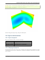
15.3 Figures and decorations
15.4 Interaction . . . . . . .
.
.
.
.
.
.
.
.
.
.
.
.
.
.
.
.
.
.
.
.
.
.
.
.
.
.
.
.
.
.
.
.
.
.
.
.
.
.
.
.
.
.
.
.
.
.
.
.
.
.
.
.
.
.
.
.
.
.
.
.
.
.
.
.
.
.
.
.
.
.
.
.
.
.
.
.
.
.
.
.
.
.
.
.
.
.
.
.
.
.
.
.
.
.
.
.
.
.
.
.
.
.
.
.
.
.
.
.
.
.
.
.
.
.
.
.
.
.
.
.
.
.
.
.
.
.
.
.
.
.
.
.
.
.
.
.
.
.
.
.
.
.
.
.
.
.
.
.
.
.
.
.
.
.
.
.
280
280
281
284
287
16 Sympy : Symbolic Mathematics in Python
16.1 First Steps with SymPy . . . . . . . .
16.2 Algebraic manipulations . . . . . . . .
16.3 Calculus . . . . . . . . . . . . . . . .
16.4 Equation solving . . . . . . . . . . . .
16.5 Linear Algebra . . . . . . . . . . . . .
.
.
.
.
.
.
.
.
.
.
.
.
.
.
.
.
.
.
.
.
.
.
.
.
.
.
.
.
.
.
.
.
.
.
.
.
.
.
.
.
.
.
.
.
.
.
.
.
.
.
.
.
.
.
.
.
.
.
.
.
.
.
.
.
.
.
.
.
.
.
.
.
.
.
.
.
.
.
.
.
.
.
.
.
.
.
.
.
.
.
.
.
.
.
.
.
.
.
.
.
.
.
.
.
.
.
.
.
.
.
.
.
.
.
.
.
.
.
.
.
.
.
.
.
.
.
.
.
.
.
.
.
.
.
.
.
.
.
.
.
.
.
.
.
.
.
.
.
.
.
.
.
.
.
.
288
289
290
291
292
293
17 scikit-learn: machine learning in Python
17.1 Loading an example dataset . . . . . . . . . . . . . . . .
17.2 Classification . . . . . . . . . . . . . . . . . . . . . . . .
17.3 Clustering: grouping observations together . . . . . . . .
17.4 Dimension Reduction with Principal Component Analysis
17.5 Putting it all together: face recognition . . . . . . . . . .
17.6 Linear model: from regression to sparsity . . . . . . . . .
17.7 Model selection: choosing estimators and their parameters
.
.
.
.
.
.
.
.
.
.
.
.
.
.
.
.
.
.
.
.
.
.
.
.
.
.
.
.
.
.
.
.
.
.
.
.
.
.
.
.
.
.
.
.
.
.
.
.
.
.
.
.
.
.
.
.
.
.
.
.
.
.
.
.
.
.
.
.
.
.
.
.
.
.
.
.
.
.
.
.
.
.
.
.
.
.
.
.
.
.
.
.
.
.
.
.
.
.
.
.
.
.
.
.
.
.
.
.
.
.
.
.
.
.
.
.
.
.
.
.
.
.
.
.
.
.
.
.
.
.
.
.
.
.
.
.
.
.
.
.
.
.
.
.
.
.
.
295
296
297
300
301
302
303
304
Index
.
.
.
.
.
.
.
.
.
.
.
.
.
.
.
.
306
iii
Python Scientific lecture notes, Release 2012.3 (EuroScipy 2012)
Contents
1
Part I
Getting started with Python for science
2
CHAPTER 1
Scientific computing with tools and
workflow
authors Fernando Perez, Emmanuelle Gouillart, Gaël Varoquaux
1.1 Why Python?
1.1.1 The scientist’s needs
• Get data (simulation, experiment control)
• Manipulate and process data.
• Visualize results... to understand what we are doing!
• Communicate results: produce figures for reports or publications, write presentations.
1.1.2 Specifications
• Rich collection of already existing bricks corresponding to classical numerical methods or basic actions: we
don’t want to re-program the plotting of a curve, a Fourier transform or a fitting algorithm. Don’t reinvent
the wheel!
• Easy to learn: computer science is neither our job nor our education. We want to be able to draw a curve,
smooth a signal, do a Fourier transform in a few minutes.
• Easy communication with collaborators, students, customers, to make the code live within a lab or a company: the code should be as readable as a book. Thus, the language should contain as few syntax symbols or
unneeded routines as possible that would divert the reader from the mathematical or scientific understanding
of the code.
• Efficient code that executes quickly... but needless to say that a very fast code becomes useless if we spend
too much time writing it. So, we need both a quick development time and a quick execution time.
• A single environment/language for everything, if possible, to avoid learning a new software for each new
problem.
1.1.3 Existing solutions
Which solutions do scientists use to work?
3
Python Scientific lecture notes, Release 2012.3 (EuroScipy 2012)
Compiled languages: C, C++, Fortran, etc.
• Advantages:
– Very fast. Very optimized compilers. For heavy computations, it’s difficult to outperform these languages.
– Some very optimized scientific libraries have been written for these languages. Example: BLAS
(vector/matrix operations)
• Drawbacks:
– Painful usage: no interactivity during development, mandatory compilation steps, verbose syntax (&,
::, }}, ; etc.), manual memory management (tricky in C). These are difficult languages for non computer scientists.
Scripting languages: Matlab
• Advantages:
– Very rich collection of libraries with numerous algorithms, for many different domains. Fast execution
because these libraries are often written in a compiled language.
– Pleasant development environment: comprehensive and well organized help, integrated editor, etc.
– Commercial support is available.
• Drawbacks:
– Base language is quite poor and can become restrictive for advanced users.
– Not free.
Other scripting languages: Scilab, Octave, Igor, R, IDL, etc.
• Advantages:
– Open-source, free, or at least cheaper than Matlab.
– Some features can be very advanced (statistics in R, figures in Igor, etc.)
• Drawbacks:
– Fewer available algorithms than in Matlab, and the language is not more advanced.
– Some software are dedicated to one domain. Ex: Gnuplot or xmgrace to draw curves. These programs
are very powerful, but they are restricted to a single type of usage, such as plotting.
What about Python?
• Advantages:
– Very rich scientific computing libraries (a bit less than Matlab, though)
– Well thought out language, allowing to write very readable and well structured code: we “code what
we think”.
– Many libraries for other tasks than scientific computing (web server management, serial port access,
etc.)
– Free and open-source software, widely spread, with a vibrant community.
• Drawbacks:
– less pleasant development environment than, for example, Matlab. (More geek-oriented).
– Not all the algorithms that can be found in more specialized software or toolboxes.
1.1. Why Python?
4
Python Scientific lecture notes, Release 2012.3 (EuroScipy 2012)
1.2 Scientific Python building blocks
Unlike Matlab, Scilab or R, Python does not come with a pre-bundled set of modules for scientific computing.
Below are the basic building blocks that can be combined to obtain a scientific computing environment:
• Python, a generic and modern computing language
– Python language: data types (string, int), flow control, data collections (lists, dictionaries), patterns, etc.
– Modules of the standard library.
– A large number of specialized modules or applications written in Python: web protocols, web framework, etc. ... and scientific computing.
– Development tools (automatic testing, documentation generation)
• IPython, an advanced Python shell http://ipython.scipy.org/moin/
• Numpy : provides powerful numerical arrays objects, and routines to manipulate them.
http://www.numpy.org/
• Scipy :
high-level data processing routines.
http://www.scipy.org/
Optimization,
regression,
interpolation,
etc
• Matplotlib : 2-D visualization, “publication-ready” plots http://matplotlib.sourceforge.net/
• Mayavi : 3-D visualization http://code.enthought.com/projects/mayavi/
1.2. Scientific Python building blocks
5
Python Scientific lecture notes, Release 2012.3 (EuroScipy 2012)
1.3 The interactive workflow: IPython and a text editor
Interactive work to test and understand algorithms: In this section, we describe an interactive workflow with
IPython that is handy to explore and understand algorithms.
Python is a general-purpose language. As such, there is not one blessed environment to work in, and not only one
way of using it. Although this makes it harder for beginners to find their way, it makes it possible for Python to be
used to write programs, in web servers, or embedded devices.
Note: Reference document for this section:
IPython user manual: http://ipython.org/ipython-doc/dev/index.html
1.3.1 Command line interaction
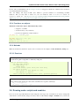
Start ipython:
In [1]: print(’Hello world’)
Hello world
Getting help:
In [2]: print ?
Type:
builtin_function_or_method
Base Class:
<type ’builtin_function_or_method’>
String Form:
<built-in function print>
Namespace:
Python builtin
Docstring:
print(value, ..., sep=’ ’, end=’\n’, file=sys.stdout)
Prints the values to a stream, or to sys.stdout by default.
Optional keyword arguments:
file: a file-like object (stream); defaults to the current sys.stdout.
sep: string inserted between values, default a space.
end: string appended after the last value, default a newline.
1.3.2 Elaboration of the algorithm in an editor
Create a file my_file.py in a text editor. Under EPD (Enthought Python Distribution), you can use Scite,
available from the start menu. Under Python(x,y), you can use Spyder. Under Ubuntu, if you don’t already have
your favorite editor, we would advise installing Stani’s Python editor. In the file, add the following
lines:
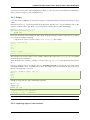
s = ’Hello world’
print(s)
Now, you can run it in IPython and explore the resulting variables:
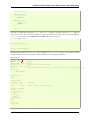
In [3]: %run my_file.py
Hello word
In [4]: s
Out[4]: ’Hello word’
In [5]: %whos
Variable
Type
Data/Info
---------------------------s
str
Hello word
1.3. The interactive workflow: IPython and a text editor
6
Python Scientific lecture notes, Release 2012.3 (EuroScipy 2012)
From a script to functions
While it is tempting to work only with scripts, that is a file full of instructions following each other, do plan
to progressively evolve the script to a set of functions:
• A script is not reusable, functions are.
• Thinking in terms of functions helps breaking the problem in small blocks.
1.3. The interactive workflow: IPython and a text editor
7
CHAPTER 2
The Python language
authors Chris Burns, Christophe Combelles, Emmanuelle Gouillart, Gaël Varoquaux
Python for scientific computing
We introduce here the Python language. Only the bare minimum necessary for getting started with Numpy
and Scipy is addressed here. To learn more about the language, consider going through the excellent tutorial
http://docs.python.org/tutorial. Dedicated books are also available, such as http://diveintopython.org/.
Python is a programming language, as are C, Fortran, BASIC, PHP, etc. Some specific features of Python are as
follows:
• an interpreted (as opposed to compiled) language. Contrary to e.g. C or Fortran, one does not compile
Python code before executing it. In addition, Python can be used interactively: many Python interpreters
are available, from which commands and scripts can be executed.
• a free software released under an open-source license: Python can be used and distributed free of charge,
even for building commercial software.
• multi-platform: Python is available for all major operating systems, Windows, Linux/Unix, MacOS X,
most likely your mobile phone OS, etc.
• a very readable language with clear non-verbose syntax
• a language for which a large variety of high-quality packages are available for various applications, from
web frameworks to scientific computing.
• a language very easy to interface with other languages, in particular C and C++.
• Some other features of the language are illustrated just below. For example, Python is an object-oriented
language, with dynamic typing (the same variable can contain objects of different types during the course
of a program).
See http://www.python.org/about/ for more information about distinguishing features of Python.
8
Python Scientific lecture notes, Release 2012.3 (EuroScipy 2012)
2.1 First steps
Start the Ipython shell (an enhanced interactive Python shell):
• by typing “ipython” from a Linux/Mac terminal, or from the Windows cmd shell,
• or by starting the program from a menu, e.g. in the Python(x,y) or EPD menu if you have installed one of
these scientific-Python suites.
If you don’t have Ipython installed on your computer, other Python shells are available, such as the plain Python
shell started by typing “python” in a terminal, or the Idle interpreter. However, we advise to use the Ipython shell
because of its enhanced features, especially for interactive scientific computing.
Once you have started the interpreter, type
>>> print "Hello, world!"
Hello, world!
The message “Hello, world!” is then displayed. You just executed your first Python instruction, congratulations!
To get yourself started, type the following stack of instructions
>>> a = 3
>>> b = 2*a
>>> type(b)
<type ’int’>
>>> print b
6
>>> a*b
18
>>> b = ’hello’
>>> type(b)
<type ’str’>
>>> b + b
’hellohello’
>>> 2*b
’hellohello’
Two variables a and b have been defined above. Note that one does not declare the type of an variable before
assigning its value. In C, conversely, one should write:
int a = 3;
In addition, the type of a variable may change, in the sense that at one point in time it can be equal to a value of
a certain type, and a second point in time, it can be equal to a value of a different type. b was first equal to an
integer, but it became equal to a string when it was assigned the value ’hello’. Operations on integers (b=2*a)
are coded natively in Python, and so are some operations on strings such as additions and multiplications, which
amount respectively to concatenation and repetition.
2.2 Basic types
2.2.1 Numerical types
Integer
>>> 1 + 1
2
>>> a = 4
Floats
2.1. First steps
9
Python Scientific lecture notes, Release 2012.3 (EuroScipy 2012)
>>> c = 2.1
Complex
>>> a = 1.5 + 0.5j
>>> a.real
1.5
>>> a.imag
0.5
Booleans
>>> 3 > 4
False
>>> test = (3 > 4)
>>> test
False
>>> type(test)
<type ’bool’>
A Python shell can therefore replace your pocket calculator, with the basic arithmetic operations +, -, *, /, %
(modulo) natively implemented:
>>> 7 * 3.
21.0
>>> 2**10
1024
>>> 8 % 3
2
Warning: Integer division
>>> 3 / 2
1
Trick: use floats:
>>> 3 / 2.
1.5
>>>
>>>
>>>
1
>>>
1.5
a = 3
b = 2
a / b
a / float(b)
• Scalar types: int, float, complex, bool:
>>> type(1)
<type ’int’>
>>> type(1.)
<type ’float’>
>>> type(1. + 0j )
<type ’complex’>
>>> a = 3
>>> type(a)
<type ’int’>
• Type conversion:
>>> float(1)
1.0
2.2. Basic types
10
Python Scientific lecture notes, Release 2012.3 (EuroScipy 2012)
2.2.2 Containers
Python provides many efficient types of containers, in which collections of objects can be stored.
Lists
A list is an ordered collection of objects, that may have different types. For example
>>> l = [1, 2, 3, 4, 5]
>>> type(l)
<type ’list’>
• Indexing: accessing individual objects contained in the list:
>>> l[2]
3
Counting from the end with negative indices:
>>> l[-1]
5
>>> l[-2]
4
Warning: Indexing starts at 0 (as in C), not at 1 (as in Fortran or Matlab)!
• Slicing: obtaining sublists of regularly-spaced elements
>>>
[1,
>>>
[3,
l
2, 3, 4, 5]
l[2:4]
4]
Warning: Note that l[start:stop] contains the elements with indices i such as start<= i < stop
(i ranging from start to stop-1). Therefore, l[start:stop] has (stop-start) elements.
Slicing syntax: l[start:stop:stride]
All slicing parameters are optional:
>>>
[4,
>>>
[1,
>>>
[1,
l[3:]
5]
l[:3]
2, 3]
l[::2]
3, 5]
Lists are mutable objects and can be modified:
>>> l[0] =
>>> l
[28, 2, 3,
>>> l[2:4]
>>> l
[28, 2, 3,
28
4, 5]
= [3, 8]
8, 5]
Note: The elements of a list may have different types:
>>>
>>>
[3,
>>>
(2,
l = [3, 2, ’hello’]
l
2, ’hello’]
l[1], l[2]
’hello’)
2.2. Basic types
11
Python Scientific lecture notes, Release 2012.3 (EuroScipy 2012)
For collections of numerical data that all have the same type, it is often more efficient to use the array type
provided by the numpy module. A NumPy array is a chunk of memory containing fixed-sized items. With
NumPy arrays, operations on elements can be faster because elements are regularly spaced in memory and more
operations are perfomed through specialized C functions instead of Python loops.
Python offers a large panel of functions to modify lists, or query them. Here are a few examples; for more details,
see http://docs.python.org/tutorial/datastructures.html#more-on-lists
Add and remove elements:
>>>
>>>
>>>
[1,
>>>
6
>>>
[1,
>>>
>>>
[1,
>>>
>>>
[1,
l = [1, 2, 3, 4, 5]
l.append(6)
l
2, 3, 4, 5, 6]
l.pop()
l
2, 3, 4, 5]
l.extend([6, 7]) # extend l, in-place
l
2, 3, 4, 5, 6, 7]
l = l[:-2]
l
2, 3, 4, 5]
Reverse l:
>>> r = l[::-1]
>>> r
[5, 4, 3, 2, 1]
Concatenate and repeat lists:
>>>
[5,
>>>
[5,
r + l
4, 3, 2, 1, 1, 2, 3, 4, 5]
2 * r
4, 3, 2, 1, 5, 4, 3, 2, 1]
Sort r (in-place):
>>> r.sort()
>>> r
[1, 2, 3, 4, 5]
Note: Methods and Object-Oriented Programming
The notation r.method() (r.sort(), r.append(3), l.pop()) is our first example of object-oriented
programming (OOP). Being a list, the object r owns the method function that is called using the notation ..
No further knowledge of OOP than understanding the notation . is necessary for going through this tutorial.
Note: Discovering methods:
In IPython: tab-completion (press tab)
In [28]: r.
r.__add__
r.__class__
r.__contains__
r.__delattr__
r.__delitem__
r.__delslice__
r.__doc__
2.2. Basic types
r.__iadd__
r.__imul__
r.__init__
r.__iter__
r.__le__
r.__len__
r.__lt__
r.__setattr__
r.__setitem__
r.__setslice__
r.__sizeof__
r.__str__
r.__subclasshook__
r.append
12
Python Scientific lecture notes, Release 2012.3 (EuroScipy 2012)
r.__eq__
r.__format__
r.__ge__
r.__getattribute__
r.__getitem__
r.__getslice__
r.__gt__
r.__hash__
r.__mul__
r.__ne__
r.__new__
r.__reduce__
r.__reduce_ex__
r.__repr__
r.__reversed__
r.__rmul__
r.count
r.extend
r.index
r.insert
r.pop
r.remove
r.reverse
r.sort
Strings
Different string syntaxes (simple, double or triple quotes):
s = ’Hello, how are you?’
s = "Hi, what’s up"
s = ’’’Hello,
how are you’’’
s = """Hi,
what’s up?"""
# tripling the quotes allows the
# the string to span more than one line
In [1]: ’Hi, what’s up ? ’
-----------------------------------------------------------File "<ipython console>", line 1
’Hi, what’s up?’
^
SyntaxError: invalid syntax
The newline character is \n, and the tab character is \t.
Strings are collections like lists. Hence they can be indexed and sliced, using the same syntax and rules.
Indexing:
>>>
>>>
’h’
>>>
’e’
>>>
’o’
a = "hello"
a[0]
a[1]
a[-1]
(Remember that negative indices correspond to counting from the right end.)
Slicing:
>>> a = "hello, world!"
>>> a[3:6] # 3rd to 6th (excluded) elements: elements 3, 4, 5
’lo,’
>>> a[2:10:2] # Syntax: a[start:stop:step]
’lo o’
>>> a[::3] # every three characters, from beginning to end
’hl r!’
Accents
and
special
characters
can
also
be
handled
http://docs.python.org/tutorial/introduction.html#unicode-strings).
in
Unicode
strings
(see
A string is an immutable object and it is not possible to modify its contents. One may however create new strings
from the original one.
In [53]: a = "hello, world!"
In [54]: a[2] = ’z’
--------------------------------------------------------------------------TypeError
Traceback (most recent call
2.2. Basic types
13
Python Scientific lecture notes, Release 2012.3 (EuroScipy 2012)
last)
/home/gouillar/travail/sgr/2009/talks/dakar_python/cours/gael/essai/source/<ipython
console> in <module>()
TypeError: ’str’ object does not support item assignment
In [55]: a.replace(’l’, ’z’, 1)
Out[55]: ’hezlo, world!’
In [56]: a.replace(’l’, ’z’)
Out[56]: ’hezzo, worzd!’
Strings have many useful methods, such as a.replace as seen above. Remember the a. object-oriented
notation and use tab completion or help(str) to search for new methods.
Note:
Python offers advanced possibilities for manipulating strings, looking for patterns or formatting. Due to lack of time this topic is not addressed here, but the interested reader is referred to
http://docs.python.org/library/stdtypes.html#string-methods and http://docs.python.org/library/string.html#newstring-formatting
• String substitution:
>>> ’An integer: %i; a float: %f; another string: %s’ % (1, 0.1, ’string’)
’An integer: 1; a float: 0.100000; another string: string’
>>> i = 102
>>> filename = ’processing_of_dataset_%03d.txt’%i
>>> filename
’processing_of_dataset_102.txt’
Dictionaries
A dictionary is basically an efficient table that maps keys to values. It is an unordered container:
>>> tel = {’emmanuelle’: 5752, ’sebastian’: 5578}
>>> tel[’francis’] = 5915
>>> tel
{’sebastian’: 5578, ’francis’: 5915, ’emmanuelle’: 5752}
>>> tel[’sebastian’]
5578
>>> tel.keys()
[’sebastian’, ’francis’, ’emmanuelle’]
>>> tel.values()
[5578, 5915, 5752]
>>> ’francis’ in tel
True
It can be used to conveniently store and retrieve values associated with a name (a string for a date, a name, etc.).
See http://docs.python.org/tutorial/datastructures.html#dictionaries for more information.
A dictionary can have keys (resp. values) with different types:
>>> d = {’a’:1, ’b’:2, 3:’hello’}
>>> d
{’a’: 1, 3: ’hello’, ’b’: 2}
More container types
• Tuples
2.2. Basic types
14
Python Scientific lecture notes, Release 2012.3 (EuroScipy 2012)
Tuples are basically immutable lists. The elements of a tuple are written between parentheses, or just separated
by commas:
>>> t = 12345, 54321, ’hello!’
>>> t[0]
12345
>>> t
(12345, 54321, ’hello!’)
>>> u = (0, 2)
• Sets: unordered, unique items:
>>> s = set((’a’, ’b’, ’c’, ’a’))
>>> s
set([’a’, ’c’, ’b’])
>>> s.difference((’a’, ’b’))
set([’c’])
A bag of Ipython tricks
•
•
•
•
Several Linux shell commands work in Ipython, such as ls,
pwd, cd, etc.
To get help about objects, functions, etc., type help object. Just type help() to get started.
Use tab-completion as much as possible: while typing the beginning of an object’s name (variable,
function, module), press the Tab key and Ipython will complete the expression to match available
names. If many names are possible, a list of names is displayed.
• History: press the up (resp. down) arrow to go through all previous (resp. next) instructions starting
with the expression on the left of the cursor (put the cursor at the beginning of the line to go through
all previous commands)
• You may log your session by using the Ipython “magic command” %logstart. Your instructions will
be saved in a file, that you can execute as a script in a different session.
In [1]: %logstart commands.log
Activating auto-logging. Current session state plus future input
saved.
Filename
: commands.log
Mode
: backup
Output logging : False
Raw input log : False
Timestamping
: False
State
: active
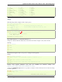
2.3 Assignment operator
Python library reference says:
Assignment statements are used to (re)bind names to values and to modify attributes or items of
mutable objects.
In short, it works as follows (simple assignment):
1. an expression on the right hand side is evaluated, the corresponding object is created/obtained
2. a name on the left hand side is assigned, or bound, to the r.h.s. object
Things to note:
• a single object can have several names bound to it:
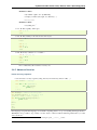
In [1]: a = [1, 2, 3]
In [2]: b = a
2.3. Assignment operator
15
Python Scientific lecture notes, Release 2012.3 (EuroScipy 2012)
In [3]:
Out[3]:
In [4]:
Out[4]:
In [5]:
Out[5]:
In [6]:
In [7]:
Out[7]:
a
[1, 2, 3]
b
[1, 2, 3]
a is b
True
b[1] = ’hi!’
a
[1, ’hi!’, 3]
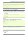
• to change a list in place, use indexing/slices:
In [1]:
In [3]:
Out[3]:
In [4]:
In [5]:
Out[5]:
In [6]:
Out[6]:
In [7]:
In [8]:
Out[8]:
In [9]:
Out[9]:
a = [1, 2, 3]
a
[1, 2, 3]
a = [’a’, ’b’, ’c’] # Creates another object.
a
[’a’, ’b’, ’c’]
id(a)
138641676
a[:] = [1, 2, 3] # Modifies object in place.
a
[1, 2, 3]
id(a)
138641676 # Same as in Out[6], yours will differ...
• the key concept here is mutable vs. immutable
– mutable objects can be changed in place
– immutable objects cannot be modified once created
A very good and detailed explanation of the above issues can be found in David M. Beazley’s article Types and
Objects in Python.
2.4 Control Flow
Controls the order in which the code is executed.
2.4.1 if/elif/else
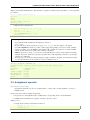
In [1]: if 2**2 == 4:
...:
print ’Obvious!’
...:
Obvious!
Blocks are delimited by indentation
Type the following lines in your Python interpreter, and be careful to respect the indentation depth. The Ipython
shell automatically increases the indentation depth after a column : sign; to decrease the indentation depth, go
four spaces to the left with the Backspace key. Press the Enter key twice to leave the logical block.
In [2]: a = 10
In [3]: if a == 1:
...:
print(1)
...: elif a == 2:
...:
print(2)
...: else:
...:
print(’A lot’)
2.4. Control Flow
16
Python Scientific lecture notes, Release 2012.3 (EuroScipy 2012)
...:
A lot
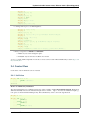
Indentation is compulsory in scripts as well. As an exercise, re-type the previous lines with the same indentation
in a script condition.py, and execute the script with run condition.py in Ipython.
2.4.2 for/range
Iterating with an index:
>>> for i in range(4):
...
print(i)
0
1
2
3
But most often, it is more readable to iterate over values:
>>> for word in (’cool’, ’powerful’, ’readable’):
...
print(’Python is %s’ % word)
Python is cool
Python is powerful
Python is readable
2.4.3 while/break/continue
Typical C-style while loop (Mandelbrot problem):
>>> z = 1 + 1j
>>> while abs(z) < 100:
...
z = z**2 + 1
>>> z
(-134+352j)
More advanced features
break out of enclosing for/while loop:
>>> z = 1 + 1j
>>> while abs(z) < 100:
...
if z.imag == 0:
...
break
...
z = z**2 + 1
continue the next iteration of a loop.:
>>> a =
>>> for
...
...
...
1.0
0.5
0.25
[1, 0, 2, 4]
element in a:
if element == 0:
continue
print 1. / element
2.4.4 Conditional Expressions
if object
2.4. Control Flow
17
Python Scientific lecture notes, Release 2012.3 (EuroScipy 2012)
Evaluates to False:
• any number equal to zero (0, 0.0, 0+0j)
• an empty container (list, tuple, set, dictionary, ...)
• False, None
Evaluates to True:
• everything else 1
a == b Tests equality, with logics:
>>> 1 == 1.
True
a is b Tests identity: both sides are the same object:
>>> 1 is 1.
False
>>> a = 1
>>> b = 1
>>> a is b
True
a in b For any collection b: b contains a
>>> b = [1, 2, 3]
>>> 2 in b
True
>>> 5 in b
False
If b is a dictionary, this tests that a is a key of b.
2.4.5 Advanced iteration
Iterate over any sequence
• You can iterate over any sequence (string, list, keys in a dictionary, lines in a file, ...):
>>> vowels = ’aeiouy’
>>> for i in ’powerful’:
...
if i in vowels:
...
print(i),
o e u
>>> message = "Hello how are you?"
>>> message.split() # returns a list
[’Hello’, ’how’, ’are’, ’you?’]
>>> for word in message.split():
...
print word
...
Hello
how
are
you?
Few languages (in particular, languages for scientific computing) allow to loop over anything but integers/indices.
With Python it is possible to loop exactly over the objects of interest without bothering with indices you often
don’t care about.
1
User-defined classes can customize those rules by overriding the special __nonzero__ method.
2.4. Control Flow
18
Python Scientific lecture notes, Release 2012.3 (EuroScipy 2012)
Warning: Not safe to modify the sequence you are iterating over.
Keeping track of enumeration number
Common task is to iterate over a sequence while keeping track of the item number.
• Could use while loop with a counter as above. Or a for loop:
>>> for i in range(0, len(words)):
...
print(i, words[i])
0 cool
1 powerful
2 readable
• But Python provides enumerate for this:
>>> words = (’cool’, ’powerful’, ’readable’)
>>> for index, item in enumerate(words):
...
print index, item
0 cool
1 powerful
2 readable
Looping over a dictionary
Use iteritems:
>>> d = {’a’: 1, ’b’:1.2, ’c’:1j}
>>> for key, val in d.iteritems():
...
print(’Key: %s has value: %s’ % (key, val))
Key: a has value: 1
Key: c has value: 1j
Key: b has value: 1.2
2.4.6 List Comprehensions
>>> [i**2 for i in range(4)]
[0, 1, 4, 9]
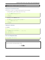
Exercise
Compute the decimals of Pi using the Wallis formula:
π=2
2.4. Control Flow
∞
Y
4i2
4i2 − 1
i=1
19
Python Scientific lecture notes, Release 2012.3 (EuroScipy 2012)
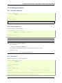
2.5 Defining functions
2.5.1 Function definition
In [56]: def test():
....:
print(’in test function’)
....:
....:
In [57]: test()
in test function
Warning: Function blocks must be indented as other control-flow blocks.
2.5.2 Return statement
Functions can optionally return values.
In [6]: def disk_area(radius):
...:
return 3.14 * radius * radius
...:
In [8]: disk_area(1.5)
Out[8]: 7.0649999999999995
Note: By default, functions return None.
Note: Note the syntax to define a function:
• the def keyword;
• is followed by the function’s name, then
• the arguments of the function are given between brackets followed by a colon.
• the function body ;
• and return object for optionally returning values.
2.5.3 Parameters
Mandatory parameters (positional arguments)
In [81]: def double_it(x):
....:
return x * 2
....:
In [82]: double_it(3)
Out[82]: 6
In [83]: double_it()
--------------------------------------------------------------------------TypeError
Traceback (most recent call last)
/Users/cburns/src/scipy2009/scipy_2009_tutorial/source/<ipython console> in <module>()
TypeError: double_it() takes exactly 1 argument (0 given)
2.5. Defining functions
20
Python Scientific lecture notes, Release 2012.3 (EuroScipy 2012)
Optional parameters (keyword or named arguments)
In [84]: def double_it(x=2):
....:
return x * 2
....:
In [85]: double_it()
Out[85]: 4
In [86]: double_it(3)
Out[86]: 6
Keyword arguments allow you to specify default values.
Warning: Default values are evaluated when the function is defined, not when it is called.
In [124]: bigx = 10
In [125]: def double_it(x=bigx):
.....:
return x * 2
.....:
In [126]: bigx = 1e9
# Now really big
In [128]: double_it()
Out[128]: 20
More involved example implementing python’s slicing:
In [98]: def slicer(seq, start=None, stop=None, step=None):
....:
"""Implement basic python slicing."""
....:
return seq[start:stop:step]
....:
In [101]: rhyme = ’one fish, two fish, red fish, blue fish’.split()
In [102]: rhyme
Out[102]: [’one’, ’fish,’, ’two’, ’fish,’, ’red’, ’fish,’, ’blue’, ’fish’]
In [103]: slicer(rhyme)
Out[103]: [’one’, ’fish,’, ’two’, ’fish,’, ’red’, ’fish,’, ’blue’, ’fish’]
In [104]: slicer(rhyme, step=2)
Out[104]: [’one’, ’two’, ’red’, ’blue’]
In [105]: slicer(rhyme, 1, step=2)
Out[105]: [’fish,’, ’fish,’, ’fish,’, ’fish’]
In [106]: slicer(rhyme, start=1, stop=4, step=2)
Out[106]: [’fish,’, ’fish,’]
The order of the keyword arguments does not matter:
In [107]: slicer(rhyme, step=2, start=1, stop=4)
Out[107]: [’fish,’, ’fish,’]
but it is good practice to use the same ordering as the function’s definition.
Keyword arguments are a very convenient feature for defining functions with a variable number of arguments,
especially when default values are to be used in most calls to the function.
2.5. Defining functions
21
Python Scientific lecture notes, Release 2012.3 (EuroScipy 2012)
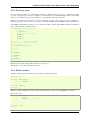
2.5.4 Passed by value
Can you modify the value of a variable inside a function? Most languages (C, Java, ...) distinguish “passing
by value” and “passing by reference”. In Python, such a distinction is somewhat artificial, and it is a bit subtle
whether your variables are going to be modified or not. Fortunately, there exist clear rules.
Parameters to functions are references to objects, which are passed by value. When you pass a variable to a
function, python passes the reference to the object to which the variable refers (the value). Not the variable itself.
If the value is immutable, the function does not modify the caller’s variable. If the value is mutable, the function
may modify the caller’s variable in-place:
>>> def try_to_modify(x, y, z):
...
x = 23
...
y.append(42)
...
z = [99] # new reference
...
print(x)
...
print(y)
...
print(z)
...
>>> a = 77
# immutable variable
>>> b = [99] # mutable variable
>>> c = [28]
>>> try_to_modify(a, b, c)
23
[99, 42]
[99]
>>> print(a)
77
>>> print(b)
[99, 42]
>>> print(c)
[28]
Functions have a local variable table. Called a local namespace.
The variable x only exists within the function foo.
2.5.5 Global variables
Variables declared outside the function can be referenced within the function:
In [114]: x = 5
In [115]: def addx(y):
.....:
return x + y
.....:
In [116]: addx(10)
Out[116]: 15
But these “global” variables cannot be modified within the function, unless declared global in the function.
This doesn’t work:
In [117]: def setx(y):
.....:
x = y
.....:
print(’x is %d’ % x)
.....:
.....:
In [118]: setx(10)
x is 10
2.5. Defining functions
22
Python Scientific lecture notes, Release 2012.3 (EuroScipy 2012)
In [120]: x
Out[120]: 5
This works:
In [121]: def setx(y):
.....:
global x
.....:
x = y
.....:
print(’x is %d’ % x)
.....:
.....:
In [122]: setx(10)
x is 10
In [123]: x
Out[123]: 10
2.5.6 Variable number of parameters
Special forms of parameters:
• *args: any number of positional arguments packed into a tuple
• **kwargs: any number of keyword arguments packed into a dictionary
In [35]: def variable_args(*args, **kwargs):
....:
print ’args is’, args
....:
print ’kwargs is’, kwargs
....:
In [36]: variable_args(’one’, ’two’, x=1, y=2, z=3)
args is (’one’, ’two’)
kwargs is {’y’: 2, ’x’: 1, ’z’: 3}
2.5.7 Docstrings
Documentation about what the function does and it’s parameters. General convention:
In [67]: def funcname(params):
....:
"""Concise one-line sentence describing the function.
....:
....:
Extended summary which can contain multiple paragraphs.
....:
"""
....:
# function body
....:
pass
....:
In [68]: funcname ?
Type:
function
Base Class: <type ’function’>
String Form:
<function funcname at 0xeaa0f0>
Namespace: Interactive
File:
/Users/cburns/src/scipy2009/.../<ipython console>
Definition: funcname(params)
Docstring:
Concise one-line sentence describing the function.
Extended summary which can contain multiple paragraphs.
Note: Docstring guidelines
2.5. Defining functions
23
Python Scientific lecture notes, Release 2012.3 (EuroScipy 2012)
For the sake of standardization, the Docstring Conventions webpage documents the semantics and conventions
associated with Python docstrings.
Also, the Numpy and Scipy modules have defined a precised standard for documenting scientific
functions, that you may want to follow for your own functions, with a Parameters section, an
Examples section, etc. See http://projects.scipy.org/numpy/wiki/CodingStyleGuidelines#docstring-standard
and http://projects.scipy.org/numpy/browser/trunk/doc/example.py#L37
2.5.8 Functions are objects
Functions are first-class objects, which means they can be:
• assigned to a variable
• an item in a list (or any collection)
• passed as an argument to another function.
In [38]: va = variable_args
In [39]: va(’three’, x=1, y=2)
args is (’three’,)
kwargs is {’y’: 2, ’x’: 1}
2.5.9 Methods
Methods are functions attached to objects. You’ve seen these in our examples on lists, dictionaries, strings, etc...
2.5.10 Exercises
Exercise: Quicksort
Implement the quicksort algorithm, as defined by wikipedia:
function quicksort(array)
var list less, greater
if length(array) < 2
return array
select and remove a pivot value pivot from array
for each x in array
if x < pivot + 1 then append x to less
else append x to greater
return concatenate(quicksort(less), pivot, quicksort(greater))
Exercise: Fibonacci sequence
Write a function that displays the n first terms of the Fibonacci sequence, defined by:
• u_0 = 1; u_1 = 1
• u_(n+2) = u_(n+1) + u_n
2.6 Reusing code: scripts and modules
For now, we have typed all instructions in the interpreter. For longer sets of instructions we need to change tack
and write the code in text files (using a text editor), that we will call either scripts or modules. Use your favorite
2.6. Reusing code: scripts and modules
24
Python Scientific lecture notes, Release 2012.3 (EuroScipy 2012)
text editor (provided it offers syntax highlighting for Python), or the editor that comes with the Scientific Python
Suite you may be using (e.g., Scite with Python(x,y)).
2.6.1 Scripts
Let us first write a script, that is a file with a sequence of instructions that are executed each time the script is
called.
Instructions may be e.g. copied-and-pasted from the interpreter (but take care to respect indentation rules!). The
extension for Python files is .py. Write or copy-and-paste the following lines in a file called test.py
message = "Hello how are you?"
for word in message.split():
print word
Let us now execute the script interactively, that is inside the Ipython interpreter. This is maybe the most common
use of scripts in scientific computing.
• in Ipython, the syntax to execute a script is %run script.py. For example,
In [1]: %run test.py
Hello
how
are
you?
In [2]: message
Out[2]: ’Hello how are you?’
The script has been executed. Moreover the variables defined in the script (such as message) are now available
inside the interpeter’s namespace.
Other interpreters also offer the possibility to execute scripts (e.g., execfile in the plain Python interpreter,
etc.).
It is also possible In order to execute this script as a standalone program, by executing the script inside a shell
terminal (Linux/Mac console or cmd Windows console). For example, if we are in the same directory as the test.py
file, we can execute this in a console:
epsilon:~/sandbox$ python test.py
Hello
how
are
you?
Standalone scripts may also take command-line arguments
In file.py:
import sys
print sys.argv
$ python file.py test arguments
[’file.py’, ’test’, ’arguments’]
Note: Don’t implement option parsing yourself. Use modules such as optparse.
2.6.2 Importing objects from modules
2.6. Reusing code: scripts and modules
25
Python Scientific lecture notes, Release 2012.3 (EuroScipy 2012)
In [1]: import os
In [2]: os
Out[2]: <module ’os’ from ’ / usr / lib / python2.6 / os.pyc ’ >
In [3]: os.listdir(’.’)
Out[3]:
[’conf.py’,
’basic_types.rst’,
’control_flow.rst’,
’functions.rst’,
’python_language.rst’,
’reusing.rst’,
’file_io.rst’,
’exceptions.rst’,
’workflow.rst’,
’index.rst’]
And also:
In [4]: from os import listdir
Importing shorthands:
In [5]: import numpy as np
Warning:
from os import *
Do not do it.
• Makes the code harder to read and understand: where do symbols come from?
• Makes it impossible to guess the functionality by the context and the name (hint: os.name is the name
of the OS), and to profit usefully from tab completion.
• Restricts the variable names you can use: os.name might override name, or vise-versa.
• Creates possible name clashes between modules.
• Makes the code impossible to statically check for undefined symbols.
Modules are thus a good way to organize code in a hierarchical way. Actually, all the scientific computing tools
we are going to use are modules:
>>> import numpy as np # data arrays
>>> np.linspace(0, 10, 6)
array([ 0.,
2.,
4.,
6.,
8., 10.])
>>> import scipy # scientific computing
In Python(x,y) software, Ipython(x,y) execute the following imports at startup:
>>>
>>>
>>>
>>>
import numpy
import numpy as np
from pylab import *
import scipy
and it is not necessary to re-import these modules.
2.6.3 Creating modules
If we want to write larger and better organized programs (compared to simple scripts), where some objects are
defined, (variables, functions, classes) and that we want to reuse several times, we have to create our own modules.
Let us create a module demo contained in the file demo.py:
2.6. Reusing code: scripts and modules
26
Python Scientific lecture notes, Release 2012.3 (EuroScipy 2012)
"A demo module."
def print_b():
"Prints b."
print ’b’
def print_a():
"Prints a."
print ’a’
c = 2
d = 2
In this file, we defined two functions print_a and print_b. Suppose we want to call the print_a function
from the interpreter. We could execute the file as a script, but since we just want to have access to the function
print_a, we are rather going to import it as a module. The syntax is as follows.
In [1]: import demo
In [2]: demo.print_a()
a
In [3]: demo.print_b()
b
Importing the module gives access to its objects, using the module.object syntax. Don’t forget to put the
module’s name before the object’s name, otherwise Python won’t recognize the instruction.
Introspection
In [4]: demo ?
Type:
module
Base Class: <type ’module’>
String Form:
<module ’demo’ from ’demo.py’>
Namespace: Interactive
File:
/home/varoquau/Projects/Python_talks/scipy_2009_tutorial/source/demo.py
Docstring:
A demo module.
In [5]: who
demo
In [6]: whos
Variable
Type
Data/Info
-----------------------------demo
module
<module ’demo’ from ’demo.py’>
In [7]: dir(demo)
Out[7]:
[’__builtins__’,
’__doc__’,
’__file__’,
’__name__’,
’__package__’,
’c’,
’d’,
’print_a’,
’print_b’]
2.6. Reusing code: scripts and modules
27
Python Scientific lecture notes, Release 2012.3 (EuroScipy 2012)
In [8]: demo.
demo.__builtins__
demo.__class__
demo.__delattr__
demo.__dict__
demo.__doc__
demo.__file__
demo.__format__
demo.__getattribute__
demo.__hash__
demo.__init__
demo.__name__
demo.__new__
demo.__package__
demo.__reduce__
demo.__reduce_ex__
demo.__repr__
demo.__setattr__
demo.__sizeof__
demo.__str__
demo.__subclasshook__
demo.c
demo.d
demo.print_a
demo.print_b
demo.py
demo.pyc
Importing objects from modules into the main namespace
In [9]: from demo import print_a, print_b
In [10]: whos
Variable
Type
Data/Info
-------------------------------demo
module
<module ’demo’ from ’demo.py’>
print_a
function
<function print_a at 0xb7421534>
print_b
function
<function print_b at 0xb74214c4>
In [11]: print_a()
a
Warning: Module caching
Modules are cached: if you modify demo.py and re-import it in the old session, you will get the
old one.
Solution:
In [10]: reload(demo)
2.6.4 ‘__main__’ and module loading
File demo2.py:
import sys
def print_a():
"Prints a."
print ’a’
print sys.argv
if __name__ == ’__main__’:
print_a()
Importing it:
In [11]: import demo2
b
In [12]: import demo2
Running it:
In [13]: %run demo2
b
a
2.6. Reusing code: scripts and modules
28
Python Scientific lecture notes, Release 2012.3 (EuroScipy 2012)
2.6.5 Scripts or modules? How to organize your code
Note: Rule of thumb
• Sets of instructions that are called several times should be written inside functions for better code reusability.
• Functions (or other bits of code) that are called from several scripts should be written inside a module,
so that only the module is imported in the different scripts (do not copy-and-paste your functions in the
different scripts!).
Note: How to import a module from a remote directory?
Many solutions exist, depending mainly on your operating system. When the import mymodule statement is
executed, the module mymodule is searched in a given list of directories. This list includes a list of installationdependent default path (e.g., /usr/lib/python) as well as the list of directories specified by the environment
variable PYTHONPATH.
The list of directories searched by Python is given by the sys.path variable
In [1]: import sys
In [2]: sys.path
Out[2]:
[’’,
’/usr/bin’,
’/usr/local/include/enthought.traits-1.1.0’,
’/usr/lib/python2.6’,
’/usr/lib/python2.6/plat-linux2’,
’/usr/lib/python2.6/lib-tk’,
’/usr/lib/python2.6/lib-old’,
’/usr/lib/python2.6/lib-dynload’,
’/usr/lib/python2.6/dist-packages’,
’/usr/lib/pymodules/python2.6’,
’/usr/lib/pymodules/python2.6/gtk-2.0’,
’/usr/lib/python2.6/dist-packages/wx-2.8-gtk2-unicode’,
’/usr/local/lib/python2.6/dist-packages’,
’/usr/lib/python2.6/dist-packages’,
’/usr/lib/pymodules/python2.6/IPython/Extensions’,
u’/home/gouillar/.ipython’]
Modules must be located in the search path, therefore you can:
• write your own modules within directories already defined in the search path (e.g.
‘/usr/local/lib/python2.6/dist-packages’). You may use symbolic links (on Linux) to keep the code
somewhere else.
• modify the environment variable PYTHONPATH to include the directories containing the user-defined
modules. On Linux/Unix, add the following line to a file read by the shell at startup (e.g. /etc/profile,
.profile)
export PYTHONPATH=$PYTHONPATH:/home/emma/user_defined_modules
On Windows, http://support.microsoft.com/kb/310519 explains how to handle environment variables.
• or modify the sys.path variable itself within a Python script.
import sys
new_path = ’/home/emma/user_defined_modules’
if new_path not in sys.path:
sys.path.append(new_path)
This method is not very robust, however, because it makes the code less portable (user-dependent path) and because
you have to add the directory to your sys.path each time you want to import from a module in this directory.
2.6. Reusing code: scripts and modules
29
Python Scientific lecture notes, Release 2012.3 (EuroScipy 2012)
See http://docs.python.org/tutorial/modules.html for more information about modules.
2.6.6 Packages
A directory that contains many modules is called a package. A package is a module with submodules (which can
have submodules themselves, etc.). A special file called __init__.py (which may be empty) tells Python that
the directory is a Python package, from which modules can be imported.
sd-2116 /usr/lib/python2.6/dist-packages/scipy $ ls
[17:07]
cluster/
io/
README.txt@
stsci/
__config__.py@ LATEST.txt@ setup.py@
__svn_version__.py@
__config__.pyc lib/
setup.pyc
__svn_version__.pyc
constants/
linalg/
setupscons.py@ THANKS.txt@
fftpack/
linsolve/
setupscons.pyc TOCHANGE.txt@
__init__.py@
maxentropy/ signal/
version.py@
__init__.pyc
misc/
sparse/
version.pyc
INSTALL.txt@
ndimage/
spatial/
weave/
integrate/
odr/
special/
interpolate/
optimize/
stats/
sd-2116 /usr/lib/python2.6/dist-packages/scipy $ cd ndimage
[17:07]
sd-2116 /usr/lib/python2.6/dist-packages/scipy/ndimage $ ls
[17:07]
doccer.py@
fourier.pyc
interpolation.py@ morphology.pyc
doccer.pyc
info.py@
interpolation.pyc _nd_image.so
setupscons.py@
filters.py@ info.pyc
measurements.py@
_ni_support.py@
setupscons.pyc
filters.pyc __init__.py@ measurements.pyc
_ni_support.pyc
fourier.py@ __init__.pyc morphology.py@
setup.py@
setup.pyc
tests/
From Ipython:
In [1]: import scipy
In [2]: scipy.__file__
Out[2]: ’/usr/lib/python2.6/dist-packages/scipy/__init__.pyc’
In [3]: import scipy.version
In [4]: scipy.version.version
Out[4]: ’0.7.0’
In [5]: import scipy.ndimage.morphology
In [6]: from scipy.ndimage import morphology
In [17]: morphology.binary_dilation ?
Type:
function
Base Class: <type ’function’>
String Form:
<function binary_dilation at 0x9bedd84>
Namespace: Interactive
File:
/usr/lib/python2.6/dist-packages/scipy/ndimage/morphology.py
Definition: morphology.binary_dilation(input, structure=None,
iterations=1, mask=None, output=None, border_value=0, origin=0,
brute_force=False)
Docstring:
Multi-dimensional binary dilation with the given structure.
2.6. Reusing code: scripts and modules
30
Python Scientific lecture notes, Release 2012.3 (EuroScipy 2012)
An output array can optionally be provided. The origin parameter
controls the placement of the filter. If no structuring element is
provided an element is generated with a squared connectivity equal
to one. The dilation operation is repeated iterations times. If
iterations is less than 1, the dilation is repeated until the
result does not change anymore. If a mask is given, only those
elements with a true value at the corresponding mask element are
modified at each iteration.
2.6.7 Good practices
Note: Good practices
• Indentation: no choice!
Indenting is compulsory in Python. Every commands block following a colon bears an additional indentation level
with respect to the previous line with a colon. One must therefore indent after def f(): or while:. At the
end of such logical blocks, one decreases the indentation depth (and re-increases it if a new block is entered, etc.)
Strict respect of indentation is the price to pay for getting rid of { or ; characters that delineate logical blocks in
other languages. Improper indentation leads to errors such as
-----------------------------------------------------------IndentationError: unexpected indent (test.py, line 2)
All this indentation business can be a bit confusing in the beginning. However, with the clear indentation, and in
the absence of extra characters, the resulting code is very nice to read compared to other languages.
• Indentation depth:
Inside your text editor, you may choose to indent with any positive number of spaces (1, 2, 3, 4, ...). However,
it is considered good practice to indent with 4 spaces. You may configure your editor to map the Tab key to a
4-space indentation. In Python(x,y), the editor Scite is already configured this way.
• Style guidelines
Long lines: you should not write very long lines that span over more than (e.g.) 80 characters. Long lines can be
broken with the \ character
>>> long_line = "Here is a very very long line \
... that we break in two parts."
Spaces
Write well-spaced code: put whitespaces after commas, around arithmetic operators, etc.:
>>> a = 1 # yes
>>> a=1 # too cramped
A certain number of rules for writing “beautiful” code (and more importantly using the same conventions as
anybody else!) are given in the Style Guide for Python Code.
• Use meaningful object names
2.7 Input and Output
To be exhaustive, here are some information about input and output in Python. Since we will use the Numpy
methods to read and write files, you may skip this chapter at first reading.
We write or read strings to/from files (other types must be converted to strings). To write in a file:
2.7. Input and Output
31
Python Scientific lecture notes, Release 2012.3 (EuroScipy 2012)
>>> f = open(’workfile’, ’w’) # opens the workfile file
>>> type(f)
<type ’file’>
>>> f.write(’This is a test \nand another test’)
>>> f.close()
To read from a file
In [1]: f = open(’workfile’, ’r’)
In [2]: s = f.read()
In [3]: print(s)
This is a test
and another test
In [4]: f.close()
For more details: http://docs.python.org/tutorial/inputoutput.html
2.7.1 Iterating over a file
In [6]: f = open(’workfile’, ’r’)
In [7]: for line in f:
...:
print line
...:
...:
This is a test
and another test
In [8]: f.close()
File modes
• Read-only: r
• Write-only: w
– Note: Create a new file or overwrite existing file.
• Append a file: a
• Read and Write: r+
• Binary mode: b
– Note: Use for binary files, especially on Windows.
2.8 Standard Library
Note: Reference document for this section:
• The Python Standard Library documentation: http://docs.python.org/library/index.html
• Python Essential Reference, David Beazley, Addison-Wesley Professional
2.8. Standard Library
32
Python Scientific lecture notes, Release 2012.3 (EuroScipy 2012)
2.8.1 os module: operating system functionality
“A portable way of using operating system dependent functionality.”
Directory and file manipulation
Current directory:
In [17]: os.getcwd()
Out[17]: ’/Users/cburns/src/scipy2009/scipy_2009_tutorial/source’
List a directory:
In [31]: os.listdir(os.curdir)
Out[31]:
[’.index.rst.swo’,
’.python_language.rst.swp’,
’.view_array.py.swp’,
’_static’,
’_templates’,
’basic_types.rst’,
’conf.py’,
’control_flow.rst’,
’debugging.rst’,
...
Make a directory:
In [32]: os.mkdir(’junkdir’)
In [33]: ’junkdir’ in os.listdir(os.curdir)
Out[33]: True
Rename the directory:
In [36]: os.rename(’junkdir’, ’foodir’)
In [37]: ’junkdir’ in os.listdir(os.curdir)
Out[37]: False
In [38]: ’foodir’ in os.listdir(os.curdir)
Out[38]: True
In [41]: os.rmdir(’foodir’)
In [42]: ’foodir’ in os.listdir(os.curdir)
Out[42]: False
Delete a file:
In [44]: fp = open(’junk.txt’, ’w’)
In [45]: fp.close()
In [46]: ’junk.txt’ in os.listdir(os.curdir)
Out[46]: True
In [47]: os.remove(’junk.txt’)
In [48]: ’junk.txt’ in os.listdir(os.curdir)
Out[48]: False
2.8. Standard Library
33
Python Scientific lecture notes, Release 2012.3 (EuroScipy 2012)
os.path: path manipulations
os.path provides common operations on pathnames.
In [70]: fp = open(’junk.txt’, ’w’)
In [71]: fp.close()
In [72]: a = os.path.abspath(’junk.txt’)
In [73]: a
Out[73]: ’/Users/cburns/src/scipy2009/scipy_2009_tutorial/source/junk.txt’
In [74]: os.path.split(a)
Out[74]: (’/Users/cburns/src/scipy2009/scipy_2009_tutorial/source’,
’junk.txt’)
In [78]: os.path.dirname(a)
Out[78]: ’/Users/cburns/src/scipy2009/scipy_2009_tutorial/source’
In [79]: os.path.basename(a)
Out[79]: ’junk.txt’
In [80]: os.path.splitext(os.path.basename(a))
Out[80]: (’junk’, ’.txt’)
In [84]: os.path.exists(’junk.txt’)
Out[84]: True
In [86]: os.path.isfile(’junk.txt’)
Out[86]: True
In [87]: os.path.isdir(’junk.txt’)
Out[87]: False
In [88]: os.path.expanduser(’~/local’)
Out[88]: ’/Users/cburns/local’
In [92]: os.path.join(os.path.expanduser(’~’), ’local’, ’bin’)
Out[92]: ’/Users/cburns/local/bin’
Running an external command
In [8]: os.system(’ls *’)
conf.py
debug_file.py demo2.py~ demo.py
demo.pyc
conf.py~ demo2.py
demo2.pyc demo.py~ my_file.py
my_file.py~
pi_wallis_image.py
Walking a directory
os.path.walk generates a list of filenames in a directory tree.
In [10]: for dirpath, dirnames, filenames in os.walk(os.curdir):
....:
for fp in filenames:
....:
print os.path.abspath(fp)
....:
....:
/Users/cburns/src/scipy2009/scipy_2009_tutorial/source/.index.rst.swo
/Users/cburns/src/scipy2009/scipy_2009_tutorial/source/.view_array.py.swp
/Users/cburns/src/scipy2009/scipy_2009_tutorial/source/basic_types.rst
/Users/cburns/src/scipy2009/scipy_2009_tutorial/source/conf.py
2.8. Standard Library
34
Python Scientific lecture notes, Release 2012.3 (EuroScipy 2012)
/Users/cburns/src/scipy2009/scipy_2009_tutorial/source/control_flow.rst
...
Environment variables:
In [9]: import os
In [11]: os.environ.keys()
Out[11]:
[’_’,
’FSLDIR’,
’TERM_PROGRAM_VERSION’,
’FSLREMOTECALL’,
’USER’,
’HOME’,
’PATH’,
’PS1’,
’SHELL’,
’EDITOR’,
’WORKON_HOME’,
’PYTHONPATH’,
...
In [12]: os.environ[’PYTHONPATH’]
Out[12]: ’.:/Users/cburns/src/utils:/Users/cburns/src/nitools:
/Users/cburns/local/lib/python2.5/site-packages/:
/usr/local/lib/python2.5/site-packages/:
/Library/Frameworks/Python.framework/Versions/2.5/lib/python2.5’
In [16]: os.getenv(’PYTHONPATH’)
Out[16]: ’.:/Users/cburns/src/utils:/Users/cburns/src/nitools:
/Users/cburns/local/lib/python2.5/site-packages/:
/usr/local/lib/python2.5/site-packages/:
/Library/Frameworks/Python.framework/Versions/2.5/lib/python2.5’
2.8.2 shutil: high-level file operations
The shutil provides useful file operations:
• shutil.rmtree: Recursively delete a directory tree.
• shutil.move: Recursively move a file or directory to another location.
• shutil.copy: Copy files or directories.
2.8.3 glob: Pattern matching on files
The glob module provides convenient file pattern matching.
Find all files ending in .txt:
In [18]: import glob
In [19]: glob.glob(’*.txt’)
Out[19]: [’holy_grail.txt’, ’junk.txt’, ’newfile.txt’]
2.8.4 sys module: system-specific information
System-specific information related to the Python interpreter.
2.8. Standard Library
35
Python Scientific lecture notes, Release 2012.3 (EuroScipy 2012)
• Which version of python are you running and where is it installed:
In [117]: sys.platform
Out[117]: ’darwin’
In [118]: sys.version
Out[118]: ’2.5.2 (r252:60911, Feb 22 2008, 07:57:53) \n
[GCC 4.0.1 (Apple Computer, Inc. build 5363)]’
In [119]: sys.prefix
Out[119]: ’/Library/Frameworks/Python.framework/Versions/2.5’
• List of command line arguments passed to a Python script:
In [100]: sys.argv
Out[100]: [’/Users/cburns/local/bin/ipython’]
sys.path is a list of strings that specifies the search path for modules. Initialized from PYTHONPATH:
In [121]: sys.path
Out[121]:
[’’,
’/Users/cburns/local/bin’,
’/Users/cburns/local/lib/python2.5/site-packages/grin-1.1-py2.5.egg’,
’/Users/cburns/local/lib/python2.5/site-packages/argparse-0.8.0-py2.5.egg’,
’/Users/cburns/local/lib/python2.5/site-packages/urwid-0.9.7.1-py2.5.egg’,
’/Users/cburns/local/lib/python2.5/site-packages/yolk-0.4.1-py2.5.egg’,
’/Users/cburns/local/lib/python2.5/site-packages/virtualenv-1.2-py2.5.egg’,
...
2.8.5 pickle: easy persistence
Useful to store arbitrary objects to a file. Not safe or fast!
In [1]: import pickle
In [2]: l = [1, None, ’Stan’]
In [3]: pickle.dump(l, file(’test.pkl’, ’w’))
In [4]: pickle.load(file(’test.pkl’))
Out[4]: [1, None, ’Stan’]
Exercise
Write a program to search your PYTHONPATH for the module site.py.
path_site
2.9 Exception handling in Python
It is highly unlikely that you haven’t yet raised Exceptions if you have typed all the previous commands of the
tutorial. For example, you may have raised an exception if you entered a command with a typo.
Exceptions are raised by different kinds of errors arising when executing Python code. In your own code, you may
also catch errors, or define custom error types.
2.9. Exception handling in Python
36
Python Scientific lecture notes, Release 2012.3 (EuroScipy 2012)
2.9.1 Exceptions
Exceptions are raised by errors in Python:
In [1]: 1/0
--------------------------------------------------------------------------ZeroDivisionError: integer division or modulo by zero
In [2]: 1 + ’e’
--------------------------------------------------------------------------TypeError: unsupported operand type(s) for +: ’int’ and ’str’
In [3]: d = {1:1, 2:2}
In [4]: d[3]
--------------------------------------------------------------------------KeyError: 3
In [5]: l = [1, 2, 3]
In [6]: l[4]
--------------------------------------------------------------------------IndexError: list index out of range
In [7]: l.foobar
--------------------------------------------------------------------------AttributeError: ’list’ object has no attribute ’foobar’
Different types of exceptions for different errors.
2.9.2 Catching exceptions
try/except
In [8]: while True:
....:
try:
....:
x = int(raw_input(’Please enter a number: ’))
....:
break
....:
except ValueError:
....:
print(’That was no valid number. Try again...’)
....:
....:
Please enter a number: a
That was no valid number. Try again...
Please enter a number: 1
In [9]: x
Out[9]: 1
try/finally
In [10]: try:
....:
x = int(raw_input(’Please enter a number: ’))
....: finally:
....:
print(’Thank you for your input’)
....:
....:
Please enter a number: a
Thank you for your input
2.9. Exception handling in Python
37
Python Scientific lecture notes, Release 2012.3 (EuroScipy 2012)
--------------------------------------------------------------------------ValueError: invalid literal for int() with base 10: ’a’
Important for resource management (e.g. closing a file)
Easier to ask for forgiveness than for permission
In [11]: def print_sorted(collection):
....:
try:
....:
collection.sort()
....:
except AttributeError:
....:
pass
....:
print(collection)
....:
....:
In [12]: print_sorted([1, 3, 2])
[1, 2, 3]
In [13]: print_sorted(set((1, 3, 2)))
set([1, 2, 3])
In [14]: print_sorted(’132’)
132
2.9.3 Raising exceptions
• Capturing and reraising an exception:
In [15]: def filter_name(name):
....:
try:
....:
name = name.encode(’ascii’)
....:
except UnicodeError, e:
....:
if name == ’Gaël’:
....:
print(’OK, Gaël’)
....:
else:
....:
raise e
....:
return name
....:
In [16]: filter_name(’Gaël’)
OK, Gaël
Out[16]: ’Ga\xc3\xabl’
In [17]: filter_name(’Stéfan’)
--------------------------------------------------------------------------UnicodeDecodeError: ’ascii’ codec can’t decode byte 0xc3 in position 2: ordinal not in range(
• Exceptions to pass messages between parts of the code:
In [17]: def achilles_arrow(x):
....:
if abs(x - 1) < 1e-3:
....:
raise StopIteration
....:
x = 1 - (1-x)/2.
....:
return x
....:
In [18]: x = 0
In [19]: while True:
....:
try:
2.9. Exception handling in Python
38
Python Scientific lecture notes, Release 2012.3 (EuroScipy 2012)
....:
....:
....:
....:
....:
x = achilles_arrow(x)
except StopIteration:
break
In [20]: x
Out[20]: 0.9990234375
Use exceptions to notify certain conditions are met (e.g. StopIteration) or not (e.g. custom error raising)
2.10 Object-oriented programming (OOP)
Python supports object-oriented programming (OOP). The goals of OOP are:
• to organize the code, and
• to re-use code in similar contexts.
Here is a small example: we create a Student class, which is an object gathering several custom functions
(methods) and variables (attributes), we will be able to use:
>>>
...
...
...
...
...
...
...
>>>
>>>
>>>
class Student(object):
def __init__(self, name):
self.name = name
def set_age(self, age):
self.age = age
def set_major(self, major):
self.major = major
anna = Student(’anna’)
anna.set_age(21)
anna.set_major(’physics’)
In the previous example, the Student class has __init__, set_age and set_major methods. Its attributes are name, age and major. We can call these methods and attributes with the following notation:
classinstance.method or classinstance.attribute. The __init__ constructor is a special
method we call with: MyClass(init parameters if any).
Now, suppose we want to create a new class MasterStudent with the same methods and attributes as the previous
one, but with an additional internship attribute. We won’t copy the previous class, but inherit from it:
>>> class MasterStudent(Student):
...
internship = ’mandatory, from March to June’
...
>>> james = MasterStudent(’james’)
>>> james.internship
’mandatory, from March to June’
>>> james.set_age(23)
>>> james.age
23
The MasterStudent class inherited from the Student attributes and methods.
Thanks to classes and object-oriented programming, we can organize code with different classes corresponding to
different objects we encounter (an Experiment class, an Image class, a Flow class, etc.), with their own methods
and attributes. Then we can use inheritance to consider variations around a base class and re-use code. Ex : from
a Flow base class, we can create derived StokesFlow, TurbulentFlow, PotentialFlow, etc.
2.10. Object-oriented programming (OOP)
39
CHAPTER 3
NumPy: creating and manipulating
numerical data
authors Emmanuelle Gouillart, Didrik Pinte, Gaël Varoquaux, and Pauli Virtanen
This chapter gives an overview of Numpy, the core tool for performant numerical computing with Python.
3.1 The numpy array object
Section contents
•
•
•
•
•
•
•
•
•
What are Numpy and numpy arrays (page 40)
Reference documentation (page 41)
Creating arrays (page 42)
Basic data types (page 44)
Basic visualization (page 44)
Indexing and slicing (page 47)
Copies and views (page 48)
Adding Axes (page 49)
Fancy indexing (page 50)
3.1.1 What are Numpy and numpy arrays
Python has built-in:
• containers: lists (costless insertion and append), dictionaries (fast lookup)
• high-level number objects: integers, floating point
Numpy is:
• extension package to Python for multi-dimensional arrays
• closer to hardware (efficiency)
• designed for scientific computation (convenience)
40
Python Scientific lecture notes, Release 2012.3 (EuroScipy 2012)
>>> import numpy as np
>>> a = np.array([0, 1, 2, 3])
>>> a
array([0, 1, 2, 3])
For example:
An array containing:
• values of an experiment/simulation at discrete time steps
• signal recorded by a measurement device, e.g. sound wave
• pixels of an image, grey-level or colour
• 3-D data measured at different X-Y-Z positions, e.g. MRI scan
• ...
Why it is useful: Memory-efficient container that provides fast numerical operations.
In [1]: l = range(1000)
In [2]: %timeit [i**2 for i in l]
1000 loops, best of 3: 403 us per loop
In [3]: a = np.arange(1000)
In [4]: %timeit a**2
100000 loops, best of 3: 12.7 us per loop
3.1.2 Reference documentation
• On the web: http://docs.scipy.org/
• Interactive help:
>>> help(np.array)
Help on built-in function array in module numpy.core.multiarray:
array(...)
array(object, dtype=None, copy=True, order=None, subok=False, ...
...
In [5]: np.array ?
String Form:<built-in function array>
Docstring:
array(object, dtype=None, copy=True, order=None, subok=False, ndmin=0, ...
...
• Looking for something:
>>> np.lookfor(’create array’)
Search results for ’create array’
--------------------------------numpy.array
Create an array.
numpy.memmap
Create a memory-map to an array stored in a *binary* file on disk.
...
In [6]: np.con* ?
np.concatenate
np.conj
3.1. The numpy array object
41
Python Scientific lecture notes, Release 2012.3 (EuroScipy 2012)
np.conjugate
np.convolve
3.1.3 Creating arrays
1-D:
>>> a = np.array([0, 1, 2, 3])
>>> a
array([0, 1, 2, 3])
>>> a.ndim
1
>>> a.shape
(4,)
>>> len(a)
4
2-D, 3-D, ...:
>>> b = np.array([[0, 1, 2], [3, 4, 5]])
# 2 x 3 array
>>> b
array([[0, 1, 2],
[3, 4, 5]])
>>> b.ndim
2
>>> b.shape
(2, 3)
>>> len(b)
# returns the size of the first dimension
2
>>> c = np.array([[[1], [2]], [[3], [4]]])
>>> c
array([[[1],
[2]],
[[3],
[4]]])
>>> c.shape
(2, 2, 1)
In practice, we rarely enter items one by one...
• Evenly spaced:
>>> import numpy as np
>>> a = np.arange(10) # 0 .. n-1 (!)
>>> a
array([0, 1, 2, 3, 4, 5, 6, 7, 8, 9])
>>> b = np.arange(1, 9, 2) # start, end (exlusive), step
>>> b
array([1, 3, 5, 7])
or by number of points:
>>> c =
>>> c
array([
>>> d =
>>> d
array([
np.linspace(0, 1, 6)
# start, end, num-points
0. , 0.2, 0.4, 0.6, 0.8, 1. ])
np.linspace(0, 1, 5, endpoint=False)
0. ,
0.2,
0.4,
0.6,
0.8])
• Common arrays:
3.1. The numpy array object
42
Python Scientific lecture notes, Release 2012.3 (EuroScipy 2012)
>>> a = np.ones((3, 3)) # reminder: (3, 3) is a tuple
>>> a
array([[ 1., 1., 1.],
[ 1., 1., 1.],
[ 1., 1., 1.]])
>>> b = np.zeros((2, 2))
>>> b
array([[ 0., 0.],
[ 0., 0.]])
>>> c = np.eye(3)
>>> c
array([[ 1., 0., 0.],
[ 0., 1., 0.],
[ 0., 0., 1.]])
>>> d = np.diag(np.array([1, 2, 3, 4]))
>>> d
array([[1, 0, 0, 0],
[0, 2, 0, 0],
[0, 0, 3, 0],
[0, 0, 0, 4]])
• np.random: random numbers (Mersenne Twister PRNG):
>>> a = np.random.rand(4)
# uniform in [0, 1]
>>> a
array([ 0.95799151, 0.14222247, 0.08777354, 0.51887998])
>>> b = np.random.randn(4)
# Gaussian
>>> b
array([ 0.37544699, -0.11425369, -0.47616538,
>>> np.random.seed(1234)
1.79664113])
# Setting the random seed
Exercise: Array creation
Create the following arrays (with correct data types):
[[
[
[
[
1
1
1
1
1
1
1
6
1
1
1
1
[[0.
[2.
[0.
[0.
[0.
[0.
0.
0.
3.
0.
0.
0.
0.
0.
0.
4.
0.
0.
1]
1]
2]
1]]
0.
0.
0.
0.
5.
0.
0.]
0.]
0.]
0.]
0.]
6.]]
Par on course: 3 statements for each
Hint: Individual array elements can be accessed similarly to a list, e.g. a[1] or a[1, 2].
Hint: Examine the docstring for diag.
Exercise: Tiling for array creation
Skim through the documentation for np.tile, and use this function to construct the array:
[[4
[2
[4
[2
3
1
3
1
4
2
4
2
3
1
3
1
4
2
4
2
3]
1]
3]
1]]
3.1. The numpy array object
43
Python Scientific lecture notes, Release 2012.3 (EuroScipy 2012)
3.1.4 Basic data types
You may have noticed that, in some instances, array elements are displayed with a trailing dot (e.g. 2. vs 2). This
is due to a difference in the data-type used:
>>> a = np.array([1, 2, 3])
>>> a.dtype
dtype(’int64’)
>>> b = np.array([1., 2., 3.])
>>> b.dtype
dtype(’float64’)
Different data-types allow us to store data more compactly in memory, but most of the time we simply work with
floating point numbers. Note that, in the example above, NumPy auto-detects the data-type from the input.
You can explicitly specify which data-type you want:
>>> c = np.array([1, 2, 3], dtype=float)
>>> c.dtype
dtype(’float64’)
The default data type is floating point:
>>> a = np.ones((3, 3))
>>> a.dtype
dtype(’float64’)
There are also other types:
Complex
>>> d = np.array([1+2j, 3+4j, 5+6*1j])
>>> d.dtype
dtype(’complex128’)
Bool
>>> e = np.array([True, False, False, True])
>>> e.dtype
dtype(’bool’)
Strings
>>> f = np.array([’Bonjour’, ’Hello’, ’Hallo’,])
>>> f.dtype
# <--- strings containing max. 7 letters
dtype(’S7’)
Much more int32/int64...
3.1.5 Basic visualization
Now that we have our first data arrays, we are going to visualize them.
Start by launching IPython in pylab mode:
$ ipython --pylab
Matplotlib is a 2D plotting package. We can import its functions as below:
>>> import matplotlib.pyplot as plt
# the tidy way
1D plotting
3.1. The numpy array object
44
Python Scientific lecture notes, Release 2012.3 (EuroScipy 2012)
>>> x = np.linspace(0, 3, 20)
>>> y = np.linspace(0, 9, 20)
>>> plt.plot(x, y)
# line plot
[<matplotlib.lines.Line2D object at ...>]
>>> plt.plot(x, y, ’o’) # dot plot
[<matplotlib.lines.Line2D object at ...>]
>>> plt.show()
# <-- shows the plot (not needed with Ipython)
9
8
7
6
5
4
3
2
1
00.0
0.5
1.0
1.5
2.0
2.5
3.0
2D arrays (such as images)
>>> image = np.random.rand(30, 30)
>>> plt.imshow(image, cmap=plt.cm.gray)
<matplotlib.image.AxesImage object at ...>
>>> plt.colorbar()
<matplotlib.colorbar.Colorbar instance at ...>
>>> plt.show()
3.1. The numpy array object
45
Python Scientific lecture notes, Release 2012.3 (EuroScipy 2012)
0
5
10
15
20
25
0
5
10
15
20
25
0.9
0.8
0.7
0.6
0.5
0.4
0.3
0.2
0.1
0.0
See Also:
More in the matplotlib chapter (page 87)
3D plotting
For 3D visualization, we can use another package: Mayavi. A quick example: start by relaunching iPython with
these options: ipython –pylab=wx (or ipython -pylab -wthread in IPython < 0.10).
In [58]:
In [61]:
Out[61]:
In [62]:
Out[62]:
from mayavi import mlab
mlab.surf(image)
<enthought.mayavi.modules.surface.Surface object at ...>
mlab.axes()
<enthought.mayavi.modules.axes.Axes object at ...>
The mayavi/mlab window that opens is interactive: by clicking on the left mouse button you can rotate the image,
3.1. The numpy array object
46
Python Scientific lecture notes, Release 2012.3 (EuroScipy 2012)
zoom with the mouse wheel, etc.
For more information on Mayavi : http://github.enthought.com/mayavi/mayavi
See Also:
More in the Mayavi chapter (page 280)
3.1.6 Indexing and slicing
The items of an array can be accessed and assigned to the same way as other Python sequences (e.g. lists)
>>> a = np.arange(10)
>>> a
array([0, 1, 2, 3, 4, 5, 6, 7, 8, 9])
>>> a[0], a[2], a[-1]
(0, 2, 9)
Warning: Indices begin at 0, like other Python sequences (and C/C++). In contrast, in Fortran or Matlab,
indices begin at 1.
For multidimensional arrays, indexes are tuples of integers:
>>> a = np.diag(np.arange(3))
>>> a
array([[0, 0, 0],
[0, 1, 0],
[0, 0, 2]])
>>> a[1, 1]
1
>>> a[2, 1] = 10 # third line, second column
>>> a
array([[ 0, 0, 0],
[ 0, 1, 0],
[ 0, 10, 2]])
>>> a[1]
array([0, 1, 0])
Note that:
• In 2D, the first dimension corresponds to rows, the second to columns.
• for multidimensional a, a[0] is interpreted by taking all elements in the unspecified dimensions.
Slicing Arrays, like other Python sequences can also be sliced:
>>> a = np.arange(10)
>>> a
array([0, 1, 2, 3, 4, 5, 6, 7, 8, 9])
>>> a[2:9:3] # [start:end:step]
array([2, 5, 8])
Note that the last index is not included!
>>> a[:4]
array([0, 1, 2, 3])
All three slice components are not required: by default, start is 0, end is the last and step is 1:
>>> a[1:3]
array([1, 2])
>>> a[::2]
array([0, 2, 4, 6, 8])
>>> a[3:]
array([3, 4, 5, 6, 7, 8, 9])
3.1. The numpy array object
47
Python Scientific lecture notes, Release 2012.3 (EuroScipy 2012)
A small illustrated summary of Numpy indexing and slicing...
3.1.7 Copies and views
A slicing operation creates a view on the original array, which is just a way of accessing array data. Thus the
original array is not copied in memory.
When modifying the view, the original array is modified as well:
>>> a = np.arange(10)
>>> a
array([0, 1, 2, 3, 4, 5, 6, 7, 8, 9])
>>> b = a[::2]; b
array([0, 2, 4, 6, 8])
>>> b[0] = 12
>>> b
array([12, 2, 4, 6, 8])
>>> a
# (!)
array([12, 1, 2, 3, 4, 5, 6, 7,
8,
9])
>>> a = np.arange(10)
>>> b = a[::2].copy() # force a copy
>>> b[0] = 12
>>> a
array([0, 1, 2, 3, 4, 5, 6, 7, 8, 9])
This behavior can be surprising at first sight... but it allows to save both memory and time.
3.1. The numpy array object
48
Python Scientific lecture notes, Release 2012.3 (EuroScipy 2012)
Warning: The transpose is a view
As a result, a matrix cannot be made symmetric in-place:
>>> a = np.ones((100, 100))
>>> a += a.T
>>> a
array([[ 2., 2., 2., ...,
[ 2., 2., 2., ...,
[ 2., 2., 2., ...,
...,
[ 3., 3., 3., ...,
[ 3., 3., 3., ...,
[ 3., 3., 3., ...,
2.,
2.,
2.,
2.,
2.,
2.,
2.],
2.],
2.],
2.,
2.,
2.,
2.,
2.,
2.,
2.],
2.],
2.]])
Worked example: Prime number sieve
Compute prime numbers in 0–99, with a sieve
• Construct a shape (100,) boolean array is_prime, filled with True in the beginning:
>>> is_prime = np.ones((100,), dtype=bool)
• Cross out 0 and 1 which are not primes:
>>> is_prime[:2] = 0
• For each integer j starting from 2, cross out its higher multiples:
>>> N_max = int(np.sqrt(len(is_prime)))
>>> for j in range(2, N_max):
...
is_prime[2*j::j] = False
• Skim through help(np.nonzero), and print the prime numbers
• Follow-up:
– Move the above code into a script file named prime_sieve.py
– Run it to check it works
– Convert the simple sieve to the sieve of Eratosthenes:
1. Skip j which are already known to not be primes
2. The first number to cross out is j 2
3.1.8 Adding Axes
Indexing with the np.newaxis object allows us to add an axis to an array:
3.1. The numpy array object
49
Python Scientific lecture notes, Release 2012.3 (EuroScipy 2012)
>>> z = np.array([1, 2, 3])
>>> z
array([1, 2, 3])
>>> z[:, np.newaxis]
array([[1],
[2],
[3]])
>>> z[np.newaxis, :]
array([[1, 2, 3]])
3.1.9 Fancy indexing
Numpy arrays can be indexed with slices, but also with boolean or integer arrays (masks). This method is called
fancy indexing. It creates copies not views.
Using boolean masks
>>> np.random.seed(3)
>>> a = np.random.random_integers(0, 20, 15)
>>> a
array([10, 3, 8, 0, 19, 10, 11, 9, 10, 6, 0, 20, 12, 7, 14])
>>> (a % 3 == 0)
array([False, True, False, True, False, False, False, True, False,
True, True, False, True, False, False], dtype=bool)
>>> mask = (a % 3 == 0)
>>> extract_from_a = a[mask] # or, a[a%3==0]
>>> extract_from_a
# extract a sub-array with the mask
array([ 3, 0, 9, 6, 0, 12])
Indexing with a mask can be very useful to assign a new value to a sub-array:
>>> a[a % 3 == 0] = -1
>>> a
array([10, -1, 8, -1, 19, 10, 11, -1, 10, -1, -1, 20, -1,
7, 14])
Indexing with an array of integers
>>> a = np.arange(10)
>>> a
array([0, 1, 2, 3, 4, 5, 6, 7, 8, 9])
Indexing can be done with an array of integers, where the same index is repeated several time:
>>> a[[2, 3, 2, 4, 2]]
array([2, 3, 2, 4, 2])
# note: [2, 3, 2, 4, 2] is a Python list
New values can be assigned with this kind of indexing:
>>> a[[9, 7]] = -10
>>> a
array([ 0,
1,
2,
3,
4,
5,
6, -10,
8, -10])
When a new array is created by indexing with an array of integers, the new array has the same shape than the array
of integers:
3.1. The numpy array object
50
Python Scientific lecture notes, Release 2012.3 (EuroScipy 2012)
>>> a = np.arange(10)
>>> idx = np.array([[3, 4], [9, 7]])
>>> a[idx]
array([[3, 4],
[9, 7]])
>>> b = np.arange(10)
The image below illustrates various fancy indexing applications
We can even use fancy indexing and broadcasting (page 58) at the same time:
>>> a = np.arange(12).reshape(3,4)
>>> a
array([[ 0, 1, 2, 3],
[ 4, 5, 6, 7],
[ 8, 9, 10, 11]])
>>> i = np.array([[0, 1], [1, 2]])
>>> a[i, 2] # same as a[i, 2*np.ones((2, 2), dtype=int)]
array([[ 2, 6],
[ 6, 10]])
3.2 Numerical operations on arrays
Section contents
•
•
•
•
•
•
•
Elementwise operations (page 51)
Basic reductions (page 53)
Broadcasting (page 58)
Array shape manipulation (page 61)
Sorting data (page 64)
Some exercises (page 65)
Summary (page 71)
3.2.1 Elementwise operations
With scalars:
3.2. Numerical operations on arrays
51
Python Scientific lecture notes, Release 2012.3 (EuroScipy 2012)
>>> a = np.array([1, 2, 3, 4])
>>> a + 1
array([2, 3, 4, 5])
>>> 2**a
array([ 2, 4, 8, 16])
All arithmetic operates elementwise:
>>> b = np.ones(4) + 1
>>> a - b
array([-1., 0., 1., 2.])
>>> a * b
array([ 2., 4., 6., 8.])
>>> j = np.arange(5)
>>> 2**(j + 1) - j
array([ 2, 3, 6, 13, 28])
Warning: Array multiplication is not matrix multiplication:
>>> c = np.ones((3, 3))
>>> c * c
array([[ 1., 1., 1.],
[ 1., 1., 1.],
[ 1., 1., 1.]])
# NOT matrix multiplication!
Note: Matrix multiplication:
>>> c.dot(c)
array([[ 3.,
[ 3.,
[ 3.,
3.,
3.,
3.,
3.],
3.],
3.]])
Comparisons:
>>> a = np.array([1, 2, 3, 4])
>>> b = np.array([4, 2, 2, 4])
>>> a == b
array([False, True, False, True], dtype=bool)
>>> a > b
array([False, False, True, False], dtype=bool)
Logical operations:
>>> a = np.array([1, 1, 0, 0], dtype=bool)
>>> b = np.array([1, 0, 1, 0], dtype=bool)
>>> np.logical_or(a, b)
array([ True, True, True, False], dtype=bool)
>>> np.logical_and(a, b)
array([ True, False, False, False], dtype=bool)
Shape mismatches:
>>> a = np.arange(4)
>>> a
array([0, 1, 2, 3])
>>> a + np.array([1, 2])
Traceback (most recent call last):
File "<stdin>", line 1, in <module>
ValueError: shape mismatch: objects cannot be broadcast to a single shape
3.2. Numerical operations on arrays
52
Python Scientific lecture notes, Release 2012.3 (EuroScipy 2012)
‘Broadcast’? We’ll return to that later (page 58).
Transposition:
>>> a = np.triu(np.ones((3, 3)), 1)
>>> a
array([[ 0., 1., 1.],
[ 0., 0., 1.],
[ 0., 0., 0.]])
>>> a.T
array([[ 0., 0., 0.],
[ 1., 0., 0.],
[ 1., 1., 0.]])
# see help(np.triu)
Note: Linear algebra
The sub-module np.linalg implements basic linear algebra, such as solving linear systems, singular value
decomposition, etc. However, it is not guaranteed to be compiled using efficient routines, and thus we recommend
the use of scipy.linalg, as detailed in section Linear algebra operations: scipy.linalg (page 108)
Exercise
Generate arrays [2**0, 2**1, 2**2, 2**3, 2**4] and a_j = 2^(3*j) - j
3.2.2 Basic reductions
Computing sums:
>>> x = np.array([1, 2, 3, 4])
>>> np.sum(x)
10
>>> x.sum()
10
Sum by rows and by columns:
>>> x = np.array([[1, 1], [2, 2]])
>>> x
array([[1, 1],
[2, 2]])
>>> x.sum(axis=0)
# columns (first dimension)
array([3, 3])
>>> x[:, 0].sum(), x[:, 1].sum()
3.2. Numerical operations on arrays
53
Python Scientific lecture notes, Release 2012.3 (EuroScipy 2012)
(3, 3)
>>> x.sum(axis=1)
# rows (second dimension)
array([2, 4])
>>> x[0, :].sum(), x[1, :].sum()
(2, 4)
Same idea in higher dimensions:
>>> x = np.random.rand(2, 2, 2)
>>> x.sum(axis=2)[0, 1]
1.14764...
>>> x[0, 1, :].sum()
1.14764...
Other reductions — works the same way (and take axis=)
• Statistics:
>>> x = np.array([1, 2, 3, 1])
>>> y = np.array([[1, 2, 3], [5, 6, 1]])
>>> x.mean()
1.75
>>> np.median(x)
1.5
>>> np.median(y, axis=-1) # last axis
array([ 2., 5.])
>>> x.std()
0.82915619758884995
# full population standard dev.
• Extrema:
>>> x = np.array([1, 3, 2])
>>> x.min()
1
>>> x.max()
3
>>> x.argmin()
0
>>> x.argmax()
1
# index of minimum
# index of maximum
• Logical operations:
>>> np.all([True, True, False])
False
>>> np.any([True, True, False])
True
Note: Can be used for array comparisons:
>>> a = np.zeros((100, 100))
>>> np.any(a != 0)
False
>>> np.all(a == a)
True
>>> a =
>>> b =
>>> c =
>>> ((a
True
np.array([1, 2, 3, 2])
np.array([2, 2, 3, 2])
np.array([6, 4, 4, 5])
<= b) & (b <= c)).all()
3.2. Numerical operations on arrays
54
Python Scientific lecture notes, Release 2012.3 (EuroScipy 2012)
• ... and many more (best to learn as you go).
Example: data statistics
Data in populations.txt describes the populations of hares and lynxes (and carrots) in northern Canada
during 20 years.
We can first plot the data:
>>> data = np.loadtxt(’data/populations.txt’)
>>> year, hares, lynxes, carrots = data.T # trick: columns to variables
>>> from matplotlib import pyplot as plt
>>> plt.axes([0.2, 0.1, 0.5, 0.8])
<matplotlib.axes.Axes object at ...>
>>> plt.plot(year, hares, year, lynxes, year, carrots)
[<matplotlib.lines.Line2D object at ...>, ...]
>>> plt.legend((’Hare’, ’Lynx’, ’Carrot’), loc=(1.05, 0.5))
<matplotlib.legend.Legend object at ...>
80000
70000
60000
Hare
Lynx
Carrot
50000
40000
30000
20000
10000
0
1900
1905 1910 1915 1920
The mean populations over time:
>>> populations = data[:, 1:]
>>> populations.mean(axis=0)
array([ 34080.95238095, 20166.66666667,
42400.
])
The sample standard deviations:
>>> populations.std(axis=0)
array([ 20897.90645809, 16254.59153691,
3322.50622558])
Which species has the highest population each year?
>>> np.argmax(populations, axis=1)
array([2, 2, 0, 0, 1, 1, 2, 2, 2, 2, 2, 2, 0, 0, 0, 1, 2, 2, 2, 2, 2])
3.2. Numerical operations on arrays
55
Python Scientific lecture notes, Release 2012.3 (EuroScipy 2012)
3.2. Numerical operations on arrays
56
Python Scientific lecture notes, Release 2012.3 (EuroScipy 2012)
Example: diffusion simulation using a random walk algorithm
What is the typical distance from the origin of a random walker after t left or right jumps?
>>> n_stories = 1000 # number of walkers
>>> t_max = 200
# time during which we follow the walker
We randomly choose all the steps 1 or -1 of the walk:
>>> t = np.arange(t_max)
>>> steps = 2 * np.random.random_integers(0, 1, (n_stories, t_max)) - 1
>>> np.unique(steps) # Verification: all steps are 1 or -1
array([-1, 1])
We build the walks by summing steps along the time:
>>> positions = np.cumsum(steps, axis=1) # axis = 1: dimension of time
>>> sq_distance = positions**2
We get the mean in the axis of the stories:
>>> mean_sq_distance = np.mean(sq_distance, axis=0)
Plot the results:
>>> plt.figure(figsize=(4, 3))
<matplotlib.figure.Figure object at ...>
>>> plt.plot(t, np.sqrt(mean_sq_distance), ’g.’, t, np.sqrt(t), ’y-’)
[<matplotlib.lines.Line2D object at ...>, <matplotlib.lines.Line2D object at ...>]
>>> plt.xlabel(r"$t$")
<matplotlib.text.Text object at ...>
>>> plt.ylabel(r"$\sqrt{\langle (\delta x)^2 \rangle}$")
<matplotlib.text.Text object at ...>
q­
(δx)2
®
16
14
12
10
8
6
4
2
00
50
100
3.2. Numerical operations on arrays
t
150
200
57
Python Scientific lecture notes, Release 2012.3 (EuroScipy 2012)
The RMS distance grows as the square root of the time!
3.2.3 Broadcasting
• Basic operations on numpy arrays (addition, etc.) are elementwise
• This works on arrays of the same size.
Nevertheless, It’s also possible to do operations on arrays of different
sizes if Numpy can transform these arrays so that they all have
the same size: this conversion is called broadcasting.
The image below gives an example of broadcasting:
Let’s verify:
>>> a = np.tile(np.arange(0, 40, 10), (3, 1)).T
>>> a
array([[ 0, 0, 0],
[10, 10, 10],
[20, 20, 20],
[30, 30, 30]])
>>> b = np.array([0, 1, 2])
>>> a + b
array([[ 0, 1, 2],
[10, 11, 12],
[20, 21, 22],
[30, 31, 32]])
An useful trick:
>>> a = np.arange(0, 40, 10)
>>> a.shape
3.2. Numerical operations on arrays
58
Python Scientific lecture notes, Release 2012.3 (EuroScipy 2012)
(4,)
>>> a = a[:, np.newaxis]
>>> a.shape
(4, 1)
>>> a
array([[ 0],
[10],
[20],
[30]])
>>> a + b
array([[ 0, 1, 2],
[10, 11, 12],
[20, 21, 22],
[30, 31, 32]])
# adds a new axis -> 2D array
We have already used broadcasting without knowing it!:
>>> a = np.ones((4, 5))
>>> a[0] = 2 # we assign an
>>> a
array([[ 2., 2., 2., 2.,
[ 1., 1., 1., 1.,
[ 1., 1., 1., 1.,
[ 1., 1., 1., 1.,
array of dimension 0 to an array of dimension 1
2.],
1.],
1.],
1.]])
Broadcasting seems a bit magical, but it is actually quite natural to use it when we want to solve a problem whose
output data is an array with more dimensions than input data.
Example
Let’s construct an array of distances (in miles) between cities of Route 66: Chicago, Springfield, Saint-Louis,
Tulsa, Oklahoma City, Amarillo, Santa Fe, Albuquerque, Flagstaff and Los Angeles.
>>> mileposts = np.array([0, 198, 303, 736, 871, 1175, 1475, 1544,
...
1913, 2448])
>>> distance_array = np.abs(mileposts - mileposts[:, np.newaxis])
>>> distance_array
array([[
0, 198, 303, 736, 871, 1175, 1475, 1544, 1913, 2448],
[ 198,
0, 105, 538, 673, 977, 1277, 1346, 1715, 2250],
[ 303, 105,
0, 433, 568, 872, 1172, 1241, 1610, 2145],
[ 736, 538, 433,
0, 135, 439, 739, 808, 1177, 1712],
[ 871, 673, 568, 135,
0, 304, 604, 673, 1042, 1577],
[1175, 977, 872, 439, 304,
0, 300, 369, 738, 1273],
[1475, 1277, 1172, 739, 604, 300,
0,
69, 438, 973],
[1544, 1346, 1241, 808, 673, 369,
69,
0, 369, 904],
[1913, 1715, 1610, 1177, 1042, 738, 438, 369,
0, 535],
[2448, 2250, 2145, 1712, 1577, 1273, 973, 904, 535,
0]])
3.2. Numerical operations on arrays
59
Python Scientific lecture notes, Release 2012.3 (EuroScipy 2012)
A lot of grid-based or network-based problems can also use broadcasting. For instance, if we want to compute the
distance from the origin of points on a 10x10 grid, we can do:
>>> x, y = np.arange(5), np.arange(5)
>>> distance = np.sqrt(x ** 2 + y[:, np.newaxis] ** 2)
>>> distance
array([[ 0.
, 1.
, 2.
, 3.
,
[ 1.
, 1.41421356, 2.23606798, 3.16227766,
[ 2.
, 2.23606798, 2.82842712, 3.60555128,
[ 3.
, 3.16227766, 3.60555128, 4.24264069,
[ 4.
, 4.12310563, 4.47213595, 5.
,
4.
],
4.12310563],
4.47213595],
5.
],
5.65685425]])
Or in color::
>>> plt.pcolor(distance)
# doctest: +ELLIPSIS
<matplotlib.collections.PolyCollection object at ...>
>>> plt.colorbar()
# doctest: +ELLIPSIS
<matplotlib.colorbar.Colorbar instance at ...>
>>> plt.axis(’equal’)
(0.0, 200.0, 0.0, 16.0)
5
4
3
2
1
0
0
1
2
3
4
5
5.4
4.8
4.2
3.6
3.0
2.4
1.8
1.2
0.6
0.0
Remark : the numpy.ogrid function allows to directly create vectors x and y of the previous example, with
two “significant dimensions”:
>>> x, y = np.ogrid[0:5, 0:5]
>>> x, y
(array([[0],
[1],
[2],
[3],
[4]]), array([[0, 1, 2, 3, 4]]))
>>> x.shape, y.shape
((5, 1), (1, 5))
3.2. Numerical operations on arrays
60
Python Scientific lecture notes, Release 2012.3 (EuroScipy 2012)
>>> distance = np.sqrt(x ** 2 + y ** 2)
So, np.ogrid is very useful as soon as we have to handle computations on a grid. On the other hand, np.mgrid
directly provides matrices full of indices for cases where we can’t (or don’t want to) benefit from broadcasting:
>>> x, y =
>>> x
array([[0,
[1,
[2,
[3,
>>> y
array([[0,
[0,
[0,
[0,
np.mgrid[0:4, 0:4]
0,
1,
2,
3,
0,
1,
2,
3,
0],
1],
2],
3]])
1,
1,
1,
1,
2,
2,
2,
2,
3],
3],
3],
3]])
However, in practice, this is rarely needed!
3.2.4 Array shape manipulation
Flattening
>>> a = np.array([[1, 2, 3], [4, 5, 6]])
>>> a.ravel()
array([1, 2, 3, 4, 5, 6])
>>> a.T
array([[1, 4],
[2, 5],
[3, 6]])
>>> a.T.ravel()
array([1, 4, 2, 5, 3, 6])
Higher dimensions: last dimensions ravel out “first”.
Reshaping
The inverse operation to flattening:
>>> a.shape
(2, 3)
>>> b = a.ravel()
>>> b.reshape((2, 3))
array([[1, 2, 3],
[4, 5, 6]])
Creating an array with a different shape, from another array:
>>> a = np.arange(36)
>>> b = a.reshape((6, 6))
>>> b
array([[ 0, 1, 2, 3, 4,
[ 6, 7, 8, 9, 10,
[12, 13, 14, 15, 16,
[18, 19, 20, 21, 22,
[24, 25, 26, 27, 28,
[30, 31, 32, 33, 34,
5],
11],
17],
23],
29],
35]])
Or,
3.2. Numerical operations on arrays
61
Python Scientific lecture notes, Release 2012.3 (EuroScipy 2012)
>>> b = a.reshape((6, -1))
# unspecified (-1) value is inferred
Views and copies
ndarray.reshape may return a view (cf help(np.reshape))), not a copy:
>>> b[0, 0] = 99
>>> a
array([99, 1, 2, 3, 4, 5, 6, 7, 8, 9, 10, 11, 12, 13, 14, 15, 16,
17, 18, 19, 20, 21, 22, 23, 24, 25, 26, 27, 28, 29, 30, 31, 32, 33,
34, 35])
Beware: reshape may also return a copy!
>>> a = np.zeros((3, 2))
>>> b = a.T.reshape(3*2)
>>> b[0] = 9
>>> a
array([[ 0., 0.],
[ 0., 0.],
[ 0., 0.]])
To understand, see the section on the memory layout of an array (page 75) below.
Dimension shuffling
>>>
>>>
(4,
>>>
5
>>>
>>>
(3,
>>>
5
a = np.arange(4*3*2).reshape(4, 3, 2)
a.shape
3, 2)
a[0, 2, 1]
b = a.transpose(1, 2, 0)
b.shape
2, 4)
b[2, 1, 0]
Also creates a view:
>>> b[2, 1, 0] = -1
>>> a[0, 2, 1]
-1
Resizing
Size of an array can be changed with ndarray.resize:
>>> a = np.arange(4)
>>> a.resize((8,))
>>> a
array([0, 1, 2, 3, 0, 0, 0, 0])
However, it must not be referred to somewhere else:
>>> b = a
>>> a.resize((4,))
...
ValueError: cannot resize an array references or is referenced
by another array in this way. Use the resize function
3.2. Numerical operations on arrays
62
Python Scientific lecture notes, Release 2012.3 (EuroScipy 2012)
Some examples of real-world use cases
Case 2.a: Calling (legacy) Fortran code
Shape-preserving functions with elementwise non-Python routines. For instance, Fortran
! 2_a_fortran_module.f90
subroutine some_function(n, a, b)
integer :: n
double precision, dimension(n), intent(in) :: a
double precision, dimension(n), intent(out) :: b
b = a + 1
end subroutine some_function
We can use f2py to wrap this fortran code in Python:
2_a_fortran_module.f90
f2py -c -m fortran_module
import numpy as np
import fortran_module
def some_function(input):
"""
Call a Fortran routine, and preserve input shape
"""
input = np.asarray(input)
# fortran_module.some_function() takes 1-D arrays!
output = fortran_module.some_function(input.ravel())
return output.reshape(input.shape)
print some_function(np.array([1, 2, 3]))
print some_function(np.array([[1, 2], [3, 4]]))
# ->
# [ 2. 3. 4.]
# [[ 2. 3.]
# [ 4. 5.]]
3.2. Numerical operations on arrays
63
Python Scientific lecture notes, Release 2012.3 (EuroScipy 2012)
Case 2.b: Block matrices and vectors (and tensors)
Vector space: quantum level ⊗ spin
ψ̂1
,
ψ̌ =
ψ̂2
ψ̂1 =
ψ1↑
ψ1↓
ψ̂2 =
ψ2↑
ψ2↓
In short: for block matrices and vectors, it can be useful to preserve the block structure.
In Numpy:
>>> psi = np.zeros((2, 2))
# dimensions: level, spin
>>> psi[0, 1] # <-- psi_{1,downarrow}
0.0
Linear operators on such block vectors have similar block structure:
ĥ11 V̂
1,↑
0
Ȟ =
,
ĥ
=
,
11
0
1,↓
V̂ † ĥ22
...
>>> H = np.zeros((2, 2, 2, 2)) # dimensions: level1, level2, spin1, spin2
>>> h_11 = H[0,0,:,:]
>>> V = H[0,1]
Doing the matrix product: get rid of the block structure, do the 4x4 matrix product, then put it back
Ȟ ψ̌
>>> def mdot(operator, psi):
...
return operator.transpose(0, 2, 1, 3).reshape(4, 4).dot(
...
psi.reshape(4)).reshape(2, 2)
I.e., reorder dimensions first to level1, spin1, level2, spin2 and then reshape => correct matrix
product.
3.2.5 Sorting data
Sorting along an axis:
>>> a = np.array([[4, 3, 5], [1, 2, 1]])
>>> b = np.sort(a, axis=1)
>>> b
array([[3, 4, 5],
[1, 1, 2]])
Note: Sorts each row separately!
In-place sort:
>>> a.sort(axis=1)
>>> a
array([[3, 4, 5],
[1, 1, 2]])
Sorting with fancy indexing:
>>> a = np.array([4, 3, 1, 2])
>>> j = np.argsort(a)
>>> j
array([2, 3, 1, 0])
3.2. Numerical operations on arrays
64
Python Scientific lecture notes, Release 2012.3 (EuroScipy 2012)
>>> a[j]
array([1, 2, 3, 4])
Finding minima and maxima:
>>>
>>>
>>>
>>>
(0,
a = np.array([4, 3, 1, 2])
j_max = np.argmax(a)
j_min = np.argmin(a)
j_max, j_min
2)
3.2.6 Some exercises
3.2. Numerical operations on arrays
65
Python Scientific lecture notes, Release 2012.3 (EuroScipy 2012)
Worked example: Framing Lena
Let’s do some manipulations on numpy arrays by starting with the famous image of Lena
(http://www.cs.cmu.edu/~chuck/lennapg/).
scipy provides a 2D array of this image with the
scipy.lena function:
>>> from scipy import misc
>>> lena = misc.lena()
Note: In older versions of scipy, you will find lena under scipy.lena()
Here are a few images we will be able to obtain with our manipulations: use different colormaps, crop the
image, change some parts of the image.
• Let’s use the imshow function of pylab to display the image.
In [3]: import pylab as plt
In [4]: lena = misc.lena()
In [5]: plt.imshow(lena)
• Lena is then displayed in false colors. A colormap must be specified for her to be displayed in grey.
In [6]: plt.imshow(lena, cmap=plt.cm.gray)
• Create an array of the image with a narrower centering : for example, remove 30 pixels from all the
borders of the image. To check the result, display this new array with imshow.
In [9]: crop_lena = lena[30:-30,30:-30]
• We will now frame Lena’s face with a black locket. For this, we need to create a mask corresponding to the pixels we want to be black. The mask is defined by this condition (y-256)**2
+ (x-256)**2
In [15]:
In [16]:
Out[16]:
In [17]:
In [18]:
y, x = np.ogrid[0:512,0:512] # x and y indices of pixels
y.shape, x.shape
((512, 1), (1, 512))
centerx, centery = (256, 256) # center of the image
mask = ((y - centery)**2 + (x - centerx)**2) > 230**2 # circle
then we assign the value 0 to the pixels of the image corresponding to the mask. The syntax is
extremely simple and intuitive:
In [19]: lena[mask] = 0
In [20]: plt.imshow(lena)
Out[20]: <matplotlib.image.AxesImage object at 0xa36534c>
• Follow-up: copy all instructions of this exercise in a script called lena_locket.py then execute
this script in IPython with %run lena_locket.py.
Change the circle to an ellipsoid.
3.2. Numerical operations on arrays
66
Python Scientific lecture notes, Release 2012.3 (EuroScipy 2012)
Exercise: Array manipulations
1. Form the 2-D array (without typing it in explicitly):
1 6
2 7
3 8
4 9
5 10
11
12
13
14
15
and generate a new array containing its 2nd and 4th rows.
2. Divide each column of the array:
>>> a = np.arange(25).reshape(5, 5)
elementwise with the array b = np.array([1., 5, 10, 15, 20]). (Hint: np.newaxis).
3. Harder one: Generate a 10 x 3 array of random numbers (in range [0,1]). For each row, pick the
number closest to 0.5.
• Use abs and argsort to find the column j closest for each row.
• Use fancy indexing to extract the numbers. (Hint: a[i,j] – the array i must contain the row
numbers corresponding to stuff in j.)
3.2. Numerical operations on arrays
67
Python Scientific lecture notes, Release 2012.3 (EuroScipy 2012)
Exercise: Data statistics
The data in populations.txt:: describes the populations of hares and lynxes (and carrots) in northern
Canada during 20 years:
>>> data = np.loadtxt(’data/populations.txt’)
>>> year, hares, lynxes, carrots = data.T # trick: columns to variables
>>> plt.axes([0.2, 0.1, 0.5, 0.8])
<matplotlib.axes.Axes object at ...>
>>> plt.plot(year, hares, year, lynxes, year, carrots)
[<matplotlib.lines.Line2D object at ...>, ...]
>>> plt.legend((’Hare’, ’Lynx’, ’Carrot’), loc=(1.05, 0.5))
<matplotlib.legend.Legend object at ...>
80000
70000
60000
50000
40000
Hare
Lynx
Carrot
30000
20000
10000
0
1900
1905 1910 1915 1920
Computes and print, based on the data in populations.txt...
1. The mean and std of the populations of each species for the years in the period.
2. Which year each species had the largest population.
3. Which species has the largest population for each year. (Hint: argsort & fancy indexing of
np.array([’H’, ’L’, ’C’]))
4. Which years any of the populations is above 50000. (Hint: comparisons and np.any)
5. The top 2 years for each species when they had the lowest populations. (Hint: argsort, fancy
indexing)
6. Compare (plot) the change in hare population (see help(np.gradient)) and the number of
lynxes. Check correlation (see help(np.corrcoef)).
... all without for-loops.
3.2. Numerical operations on arrays
68
Python Scientific lecture notes, Release 2012.3 (EuroScipy 2012)
Exercise: Crude integral approximations
Write a function f(a, b, c) that returns ab − c. Form a 24x12x6 array containing its values in parameter
ranges [0,1] x [0,1] x [0,1].
Approximate the 3-d integral
Z
0
1
Z
0
1
Z
1
(ab − c)da db dc
0
over this volume with the mean. The exact result is: ln 2 − 12 ≈ 0.1931 . . . — what is your relative error?
(Hints: use elementwise operations and broadcasting. You can make np.ogrid give a number of points in
given range with np.ogrid[0:1:20j].)
Reminder Python functions:
def f(a, b, c):
return some_result
3.2. Numerical operations on arrays
69
Python Scientific lecture notes, Release 2012.3 (EuroScipy 2012)
Exercise: Mandelbrot set
1.5
1.0
0.5
0.0
0.5
1.0
1.52.0
1.5
1.0
0.5 0.0
0.5
1.0
Write a script that computes the Mandelbrot fractal. The Mandelbrot iteration:
N_max = 50
some_threshold = 50
c = x + 1j*y
for j in xrange(N_max):
z = z**2 + c
Point (x, y) belongs to the Mandelbrot set if |c| < some_threshold.
Do this computation by:
1. Construct a grid of c = x + 1j*y values in range [-2, 1] x [-1.5, 1.5]
2. Do the iteration
3. Form the 2-d boolean mask indicating which points are in the set
4. Save the result to an image with:
>>> import matplotlib.pyplot as plt
>>> plt.imshow(mask.T, extent=[-2, 1, -1.5, 1.5])
<matplotlib.image.AxesImage object at ...>
>>> plt.gray()
>>> plt.savefig(’mandelbrot.png’)
3.2. Numerical operations on arrays
70
Python Scientific lecture notes, Release 2012.3 (EuroScipy 2012)
Exercise: Markov chain
Markov chain transition matrix P, and probability distribution on the states p:
1. 0 <= P[i,j] <= 1: probability to go from state i to state j
2. Transition rule: pnew = P T pold
3. all(sum(P, axis=1) == 1), p.sum() == 1: normalization
Write a script that works with 5 states, and:
• Constructs a random matrix, and normalizes each row so that it is a transition matrix.
• Starts from a random (normalized) probability distribution p and takes 50 steps => p_50
• Computes the stationary distribution: the eigenvector of P.T with eigenvalue 1 (numerically: closest to 1) => p_stationary
Remember to normalize the eigenvector — I didn’t...
• Checks if p_50 and p_stationary are equal to tolerance 1e-5
Toolbox: np.random.rand, .dot(), np.linalg.eig, reductions, abs(), argmin,
comparisons, all, np.linalg.norm, etc.
3.2.7 Summary
What do you need to know to get started?
• Know how to create arrays : array, arange, ones, zeros.
• Know the shape of the array with array.shape, then use slicing to obtain different views of the array:
array[::2], etc. Adjust the shape of the array using reshape or flatten it with ravel.
• Obtain a subset of the elements of an array and/or modify their values with masks:
>>> a[a < 0] = 0
• Know miscellaneous operations on arrays, such as finding the mean or max (array.max(),
array.mean()). No need to retain everything, but have the reflex to search in the documentation (online
docs, help(), lookfor())!!
• For advanced use: master the indexing with arrays of integers, as well as broadcasting. Know more Numpy
functions to handle various array operations.
3.3 More elaborate arrays
3.3. More elaborate arrays
71
Python Scientific lecture notes, Release 2012.3 (EuroScipy 2012)
Section contents
•
•
•
•
More data types (page 72)
Structured data types (page 73)
maskedarray: dealing with (propagation of) missing data (page 74)
Under the hood: the memory layout of a numpy array (page 75)
3.3.1 More data types
Casting
“Bigger” type wins in mixed-type operations:
>>> np.array([1, 2, 3]) + 1.5
array([ 2.5, 3.5, 4.5])
Assignment never changes the type!
>>> a = np.array([1, 2, 3])
>>> a.dtype
dtype(’int64’)
>>> a[0] = 1.9
# <-- float is truncated to integer
>>> a
array([1, 2, 3])
Forced casts:
>>> a = np.array([1.7, 1.2, 1.6])
>>> b = a.astype(int) # <-- truncates to integer
>>> b
array([1, 1, 1])
Rounding:
>>> a =
>>> b =
>>> b
array([
>>> c =
>>> c
array([
np.array([1.2, 1.5, 1.6, 2.5, 3.5, 4.5])
np.around(a)
# still floating-point
1., 2., 2., 2., 4., 4.])
np.around(a).astype(int)
1, 2, 2, 2, 4, 4])
Different data type sizes
Integers (signed):
int8
int16
int32
int64
8 bits
16 bits
32 bits (same as int on 32-bit platform)
64 bits (same as int on 64-bit platform)
>>> np.array([1], dtype=int).dtype
dtype(’int64’)
>>> np.iinfo(np.int32).max, 2**31 - 1
(2147483647, 2147483647)
>>> np.iinfo(np.int64).max, 2**63 - 1
(9223372036854775807, 9223372036854775807L)
Unsigned integers:
3.3. More elaborate arrays
72
Python Scientific lecture notes, Release 2012.3 (EuroScipy 2012)
uint8
uint16
uint32
uint64
8 bits
16 bits
32 bits
64 bits
>>> np.iinfo(np.uint32).max, 2**32 - 1
(4294967295, 4294967295)
>>> np.iinfo(np.uint64).max, 2**64 - 1
(18446744073709551615L, 18446744073709551615L)
Floating-point numbers:
float16
float32
float64
float96
float128
16 bits
32 bits
64 bits (same as float)
96 bits, platform-dependent (same as np.longdouble)
128 bits, platform-dependent (same as np.longdouble)
>>> np.finfo(np.float32).eps
1.1920929e-07
>>> np.finfo(np.float64).eps
2.2204460492503131e-16
>>> np.float32(1e-8) + np.float32(1) == 1
True
>>> np.float64(1e-8) + np.float64(1) == 1
False
Complex floating-point numbers:
complex64
complex128
complex192
complex256
two 32-bit floats
two 64-bit floats
two 96-bit floats, platform-dependent
two 128-bit floats, platform-dependent
Smaller data types
If you don’t know you need special data types, then you probably don’t.
Comparison on using float32 instead of float64:
• Half the size in memory and on disk
• Half the memory bandwidth required (may be a bit faster in some operations)
In [1]: a = np.zeros((1e6,), dtype=np.float64)
In [2]: b = np.zeros((1e6,), dtype=np.float32)
In [3]: %timeit a*a
1000 loops, best of 3: 1.78 ms per loop
In [4]: %timeit b*b
1000 loops, best of 3: 1.07 ms per loop
• But: bigger rounding errors — sometimes in surprising places (i.e., don’t use them unless you really
need them)
3.3.2 Structured data types
sensor_code (4-character string)
position (float)
value (float)
3.3. More elaborate arrays
73
Python Scientific lecture notes, Release 2012.3 (EuroScipy 2012)
>>> samples = np.zeros((6,), dtype=[(’sensor_code’, ’S4’),
...
(’position’, float), (’value’, float)])
>>> samples.ndim
1
>>> samples.shape
(6,)
>>> samples.dtype.names
(’sensor_code’, ’position’, ’value’)
>>> samples[:] = [(’ALFA’,
1, 0.37), (’BETA’, 1, 0.11), (’TAU’, 1,
0.13),
...
(’ALFA’, 1.5, 0.37), (’ALFA’, 3, 0.11), (’TAU’, 1.2, 0.13)]
>>> samples
array([(’ALFA’, 1.0, 0.37), (’BETA’, 1.0, 0.11), (’TAU’, 1.0, 0.13),
(’ALFA’, 1.5, 0.37), (’ALFA’, 3.0, 0.11), (’TAU’, 1.2, 0.13)],
dtype=[(’sensor_code’, ’|S4’), (’position’, ’<f8’), (’value’, ’<f8’)])
Field access works by indexing with field names:
>>> samples[’sensor_code’]
array([’ALFA’, ’BETA’, ’TAU’, ’ALFA’, ’ALFA’, ’TAU’],
dtype=’|S4’)
>>> samples[’value’]
array([ 0.37, 0.11, 0.13, 0.37, 0.11, 0.13])
>>> samples[0]
(’ALFA’, 1.0, 0.37)
>>> samples[0][’sensor_code’] = ’TAU’
>>> samples[0]
(’TAU’, 1.0, 0.37)
Multiple fields at once:
>>> samples[[’position’, ’value’]]
array([(1.0, 0.37), (1.0, 0.11), (1.0, 0.13), (1.5, 0.37), (3.0, 0.11),
(1.2, 0.13)],
dtype=[(’position’, ’<f8’), (’value’, ’<f8’)])
Fancy indexing works, as usual:
>>> samples[samples[’sensor_code’] == ’ALFA’]
array([(’ALFA’, 1.5, 0.37), (’ALFA’, 3.0, 0.11)],
dtype=[(’sensor_code’, ’|S4’), (’position’, ’<f8’), (’value’, ’<f8’)])
Note: There are a bunch of other syntaxes for constructing structured arrays, see here and here.
3.3.3 maskedarray: dealing with (propagation of) missing data
• For floats one could use NaN’s, but masks work for all types:
>>> x = np.ma.array([1, 2, 3, 4], mask=[0, 1, 0, 1])
>>> x
masked_array(data = [1 -- 3 --],
mask = [False True False True],
fill_value = 999999)
>>> y = np.ma.array([1, 2, 3, 4], mask=[0, 1, 1, 1])
>>> x + y
masked_array(data = [2 -- -- --],
mask = [False True True True],
fill_value = 999999)
3.3. More elaborate arrays
74
Python Scientific lecture notes, Release 2012.3 (EuroScipy 2012)
• Masking versions of common functions:
>>> np.ma.sqrt([1, -1, 2, -2])
masked_array(data = [1.0 -- 1.41421356237 --],
mask = [False True False True],
fill_value = 1e+20)
Note: There are other useful array siblings (page 184)
3.3.4 Under the hood: the memory layout of a numpy array
A numpy array is:
block of memory + indexing scheme + data type descriptor
• raw data
• how to locate an element
• how to interpret an element
Block of memory
>>> x = np.array([1, 2, 3, 4], dtype=np.int32)
>>> x.data
<read-write buffer for ..., size 16, offset 0 at ...>
>>> str(x.data)
’\x01\x00\x00\x00\x02\x00\x00\x00\x03\x00\x00\x00\x04\x00\x00\x00’
Memory address of the data:
>>> x.__array_interface__[’data’][0]
159755776
Reminder: two ndarrays may share the same memory:
>>> x = np.array([1,2,3,4])
>>> y = x[:]
>>> x[0] = 9
>>> y
array([9, 2, 3, 4])
>>> y.base is x
True
Memory does not need to be owned by an ndarray:
3.3. More elaborate arrays
75
Python Scientific lecture notes, Release 2012.3 (EuroScipy 2012)
>>> x = ’\x01\x02\x03\x04’
>>> y = np.frombuffer(x, dtype=np.int8)
>>> y
array([1, 2, 3, 4], dtype=int8)
>>> y.data
<read-only buffer for ..., size 4, offset 0 at ...>
>>> y.base is x
True
>>> y.flags
C_CONTIGUOUS : True
F_CONTIGUOUS : True
OWNDATA : False
WRITEABLE : False
ALIGNED : True
UPDATEIFCOPY : False
The owndata and writeable flags indicate status of the memory block.
Indexing scheme: strides
The question
>>> x = np.array([[1, 2, 3],
...
[4, 5, 6],
...
[7, 8, 9]], dtype=np.int8)
>>> str(x.data)
’\x01\x02\x03\x04\x05\x06\x07\x08\t’
At which byte in x.data does the item x[1, 2] begin?
The answer (in Numpy)
• strides: the number of bytes to jump to find the next element
• 1 stride per dimension
>>> x.strides
(3, 1)
>>> byte_offset = 3*1 + 1*2
>>> x.data[byte_offset]
’\x06’
>>> x[1, 2]
6
# to find x[1, 2]
• simple, flexible
C and Fortran order
>>> x = np.array([[1, 2, 3],
...
[4, 5, 6],
...
[7, 8, 9]], dtype=np.int16, order=’C’)
>>> x.strides
(6, 2)
>>> str(x.data)
’\x01\x00\x02\x00\x03\x00\x04\x00\x05\x00\x06\x00\x07\x00\x08\x00\t\x00’
• Need to jump 6 bytes to find the next row
• Need to jump 2 bytes to find the next column
3.3. More elaborate arrays
76
Python Scientific lecture notes, Release 2012.3 (EuroScipy 2012)
>>> y = np.array(x, order=’F’)
>>> y.strides
(2, 6)
>>> str(y.data)
’\x01\x00\x04\x00\x07\x00\x02\x00\x05\x00\x08\x00\x03\x00\x06\x00\t\x00’
• Need to jump 2 bytes to find the next row
• Need to jump 6 bytes to find the next column
• Similarly to higher dimensions:
– C: last dimensions vary fastest (= smaller strides)
– F: first dimensions vary fastest
shape = (d1 , d2 , ..., dn )
strides = (s1 , s2 , ..., sn )
sC
j = dj+1 dj+2 ...dn × itemsize
sF
j = d1 d2 ...dj−1 × itemsize
Slicing
• Everything can be represented by changing only shape, strides, and possibly adjusting the data
pointer!
• Never makes copies of the data
>>> x = np.array([1, 2, 3, 4, 5, 6], dtype=np.int32)
>>> y = x[::-1]
>>> y
array([6, 5, 4, 3, 2, 1], dtype=int32)
>>> y.strides
(-4,)
>>> y = x[2:]
>>> y.__array_interface__[’data’][0] - x.__array_interface__[’data’][0]
8
>>> x = np.zeros((10, 10, 10), dtype=np.float)
>>> x.strides
(800, 80, 8)
>>> x[::2,::3,::4].strides
(1600, 240, 32)
• Similarly, transposes never make copies (it just swaps strides)
>>> x = np.zeros((10, 10, 10), dtype=np.float)
>>> x.strides
(800, 80, 8)
>>> x.T.strides
(8, 80, 800)
Reshaping
But: not all reshaping operations can be represented by playing with strides.
>>>
>>>
>>>
(1,
a = np.arange(6, dtype=np.int8).reshape(3, 2)
b = a.T
b.strides
2)
3.3. More elaborate arrays
77
Python Scientific lecture notes, Release 2012.3 (EuroScipy 2012)
So far, so good. However:
>>> str(a.data)
’\x00\x01\x02\x03\x04\x05’
>>> b
array([[0, 2, 4],
[1, 3, 5]], dtype=int8)
>>> c = b.reshape(3*2)
>>> c
array([0, 2, 4, 1, 3, 5], dtype=int8)
Here, there is no way to represent the array c given one stride and the block of memory for a. Therefore, the
reshape operation needs to make a copy here.
Summary
• Numpy array: block of memory + indexing scheme + data type description
• Indexing: strides
byte_position = np.sum(arr.strides * indices)
• Various tricks can you do by playing with the strides (stuff for an advanced tutorial it is)
While it is off topic in a chapter on numpy, let’s take a moment to recall good coding practice, which really do pay
off in the long run:
Good practices
• Explicit variable names (no need of a comment to explain what is in the variable)
• Style: spaces after commas, around =, etc.
A certain number of rules for writing “beautiful” code (and, more importantly, using the same conventions as everybody else!) are given in the Style Guide for Python Code and the Docstring Conventions
page (to manage help strings).
• Except some rare cases, variable names and comments in English.
3.4 Advanced operations
Section contents
• Polynomials (page 78)
• Loading data files (page 80)
3.4.1 Polynomials
Numpy also contains polynomials in different bases:
For example, 3x2 + 2x − 1
>>> p = np.poly1d([3, 2, -1])
>>> p(0)
-1
>>> p.roots
array([-1.
, 0.33333333])
>>> p.order
2
3.4. Advanced operations
78
Python Scientific lecture notes, Release 2012.3 (EuroScipy 2012)
>>> x = np.linspace(0, 1, 20)
>>> y = np.cos(x) + 0.3*np.random.rand(20)
>>> p = np.poly1d(np.polyfit(x, y, 3))
>>> t = np.linspace(0, 1, 200)
>>> plt.plot(x, y, ’o’, t, p(t), ’-’)
[<matplotlib.lines.Line2D object at ...>, <matplotlib.lines.Line2D object at ...>]
1.3
1.2
1.1
1.0
0.9
0.8
0.70.0
0.2
0.4
0.6
0.8
1.0
See http://docs.scipy.org/doc/numpy/reference/routines.polynomials.poly1d.html for more.
More polynomials (with more bases)
Numpy also has a more sophisticated polynomial interface, which supports e.g. the Chebyshev basis.
3x2 + 2x − 1
>>> p = np.polynomial.Polynomial([-1, 2, 3]) # coefs in different order!
>>> p(0)
-1.0
>>> p.roots()
array([-1.
, 0.33333333])
>>> p.degree() # In general polynomials do not always expose ’order’
2
Example using polynomials in Chebyshev basis, for polynomials in range [-1, 1]:
>>> x = np.linspace(-1, 1, 2000)
>>> y = np.cos(x) + 0.3*np.random.rand(2000)
>>> p = np.polynomial.Chebyshev.fit(x, y, 90)
>>> t = np.linspace(-1, 1, 200)
>>> plt.plot(x, y, ’r.’)
3.4. Advanced operations
79
Python Scientific lecture notes, Release 2012.3 (EuroScipy 2012)
[<matplotlib.lines.Line2D object at ...>]
>>> plt.plot(t, p(t), ’k-’, lw=3)
[<matplotlib.lines.Line2D object at ...>]
1.3
1.2
1.1
1.0
0.9
0.8
0.7
0.6
0.51.0
0.5
0.0
0.5
1.0
The Chebyshev polynomials have some advantages in interpolation.
3.4.2 Loading data files
Text files
Example: populations.txt:
1900
1901
1902
...
30e3
47.2e3
70.2e3
4e3
6.1e3
9.8e3
48300
48200
41500
>>> data = np.loadtxt(’data/populations.txt’)
>>> data
array([[ 1900., 30000.,
4000., 48300.],
[ 1901., 47200.,
6100., 48200.],
[ 1902., 70200.,
9800., 41500.],
...
>>> np.savetxt(’pop2.txt’, data)
>>> data2 = np.loadtxt(’pop2.txt’)
Note: If you have a complicated text file, what you can try are:
• np.genfromtxt
3.4. Advanced operations
80
Python Scientific lecture notes, Release 2012.3 (EuroScipy 2012)
• Using Python’s I/O functions and e.g. regexps for parsing (Python is quite well suited for this)
Navigating the filesystem with Ipython
In [1]: pwd
# show current directory
’/home/user/stuff/2011-numpy-tutorial’
In [2]: cd ex
’/home/user/stuff/2011-numpy-tutorial/ex’
In [3]: ls
populations.txt species.txt
Images
Using Matplotlib:
>>> img = plt.imread(’data/elephant.png’)
>>> img.shape, img.dtype
((200, 300, 3), dtype(’float32’))
>>> plt.imshow(img)
<matplotlib.image.AxesImage object at ...>
>>> plt.savefig(’plot.png’)
>>> plt.imsave(’red_elephant’, img[:,:,0], cmap=plt.cm.gray)
This saved only one channel (of RGB):
>>> plt.imshow(plt.imread(’red_elephant.png’))
<matplotlib.image.AxesImage object at ...>
Other libraries:
>>> from scipy.misc import imsave
>>> imsave(’tiny_elephant.png’, img[::6,::6])
>>> plt.imshow(plt.imread(’tiny_elephant.png’), interpolation=’nearest’)
<matplotlib.image.AxesImage object at ...>
3.4. Advanced operations
81
Python Scientific lecture notes, Release 2012.3 (EuroScipy 2012)
0
5
10
15
20
25
30
0
10
20
30
40
Numpy’s own format
Numpy has its own binary format, not portable but with efficient I/O:
>>> data = np.ones((3, 3))
>>> np.save(’pop.npy’, data)
>>> data3 = np.load(’pop.npy’)
Well-known (& more obscure) file formats
• HDF5: h5py, PyTables
• NetCDF: scipy.io.netcdf_file, netcdf4-python, ...
• Matlab: scipy.io.loadmat, scipy.io.savemat
• MatrixMarket: scipy.io.mmread, scipy.io.mmread
... if somebody uses it, there’s probably also a Python library for it.
Exercise: Text data files
Write a Python script that loads data from populations.txt:: and drop the last column and the first 5
rows. Save the smaller dataset to pop2.txt.
3.4. Advanced operations
82
CHAPTER 4
Getting help and finding
documentation
author Emmanuelle Gouillart
Rather than knowing all functions in Numpy and Scipy, it is important to find rapidly information throughout the
documentation and the available help. Here are some ways to get information:
• In Ipython, help function opens the docstring of the function. Only type the beginning of the function’s name and use tab completion to display the matching functions.
In [204]: help np.v
np.vander
np.vdot
np.var
np.vectorize
np.version
np.void
np.void0
np.vsplit
np.vstack
In [204]: help np.vander
In Ipython it is not possible to open a separated window for help and documentation; however one can always
open a second Ipython shell just to display help and docstrings...
• Numpy’s and Scipy’s documentations can be browsed online on http://docs.scipy.org/doc.
The search button is quite useful inside the reference documentation of the two packages
(http://docs.scipy.org/doc/numpy/reference/ and http://docs.scipy.org/doc/scipy/reference/).
Tutorials on various topics as well as the complete API with all docstrings are found on this website.
83
Python Scientific lecture notes, Release 2012.3 (EuroScipy 2012)
• Numpy’s and Scipy’s documentation is enriched and updated on a regular basis by users on a wiki
http://docs.scipy.org/numpy/. As a result, some docstrings are clearer or more detailed on the wiki, and
you may want to read directly the documentation on the wiki instead of the official documentation website.
Note that anyone can create an account on the wiki and write better documentation; this is an easy way to
contribute to an open-source project and improve the tools you are using!
• Scipy’s cookbook http://www.scipy.org/Cookbook gives recipes on many common problems frequently encountered, such as fitting data points, solving ODE, etc.
• Matplotlib’s website http://matplotlib.sourceforge.net/ features a very nice gallery with a large number of
plots, each of them shows both the source code and the resulting plot. This is very useful for learning by
example. More standard documentation is also available.
• Mayavi’s website http://code.enthought.com/projects/mayavi/docs/development/html/mayavi/ also has a
very nice gallery of examples http://code.enthought.com/projects/mayavi/docs/development/html/mayavi/auto/examples.html
in which one can browse for different visualization solutions.
84
Python Scientific lecture notes, Release 2012.3 (EuroScipy 2012)
Finally, two more “technical” possibilities are useful as well:
• In Ipython, the magical function %psearch search for objects matching patterns. This is useful if, for
example, one does not know the exact name of a function.
In [3]: import numpy as np
In [4]: %psearch np.diag*
np.diag
np.diagflat
np.diagonal
• numpy.lookfor looks for keywords inside the docstrings of specified modules.
In [45]: numpy.lookfor(’convolution’)
Search results for ’convolution’
-------------------------------numpy.convolve
Returns the discrete, linear convolution of two one-dimensional
sequences.
numpy.bartlett
Return the Bartlett window.
numpy.correlate
Discrete, linear correlation of two 1-dimensional sequences.
In [46]: numpy.lookfor(’remove’, module=’os’)
Search results for ’remove’
--------------------------os.remove
remove(path)
os.removedirs
removedirs(path)
os.rmdir
rmdir(path)
os.unlink
unlink(path)
os.walk
Directory tree generator.
• If everything listed above fails (and Google doesn’t have the answer)... don’t despair! Write to the mailinglist suited to your problem: you should have a quick answer if you describe your problem well. Experts on
scientific python often give very enlightening explanations on the mailing-list.
– Numpy discussion ([email protected]): all about numpy arrays, manipulating them, indexation questions, etc.
85
Python Scientific lecture notes, Release 2012.3 (EuroScipy 2012)
– SciPy Users List ([email protected]): scientific computing with Python, high-level data processing, in particular with the scipy package.
– [email protected] for plotting with matplotlib.
86
CHAPTER 5
Matplotlib
author Mike Müller
5.1 Introduction
matplotlib is probably the single most used Python package for 2D-graphics. It provides both a very quick
way to visualize data from Python and publication-quality figures in many formats. We are going to explore
matplotlib in interactive mode covering most common cases. We also look at the class library which is provided
with an object-oriented interface.
5.2 IPython and the pylab mode
5.2.1 IPython
IPython is an enhanced interactive Python shell that has lots of interesting features including named inputs and
outputs, access to shell commands, improved debugging and many more. When we start it with the command line
argument -pylab (--pylab since IPython version 0.12), it allows interactive matplotlib sessions that has
Matlab/Mathematica-like functionality.
5.2.2 pylab
pylab provides a procedural interface to the matplotlib object-oriented plotting library. It is modeled closely
after Matlab(TM). Therefore, the majority of plotting commands in pylab has Matlab(TM) analogs with similar
arguments. Important commands are explained with interactive examples.
5.3 Simple Plots
Let’s start an interactive session:
$ ipython -pylab
This brings us to the IPython prompt:
IPython 0.8.1 -- An enhanced Interactive Python.
?
-> Introduction to IPython’s features.
%magic -> Information about IPython’s ’magic’ % functions.
87
Python Scientific lecture notes, Release 2012.3 (EuroScipy 2012)
help
-> Python’s own help system.
object? -> Details about ’object’. ?object also works, ?? prints more.
Welcome to pylab, a matplotlib-based Python environment.
For more information, type ’help(pylab)’.
In [1]:
Now we can make our first, really simple plot:
In [1]:
In [2]:
In [3]:
Out[3]:
import numpy as np
import pylab as pl
pl.plot(np.range(10))
[<matplotlib.lines.Line2D instance at 0x01AA26E8>]
In [4]:
The numbers form 0 through 9 are plotted:
Note: In the following, we use the Python prompt “>>>” rather than the IPython one, as it facilitates copy-pasting
in IPython (using the %doctest_mode).
Now we can interactively add features to or plot:
>>> pl.xlabel(’measured’)
<matplotlib.text.Text instance at ...>
>>> pl.ylabel(’calculated’)
<matplotlib.text.Text instance at ...>
>>> pl.title(’Measured vs. calculated’) +ELLIPSIS
<matplotlib.text.Text instance at ...>
>>> pl.grid(True)
We get a reference to our plot:
>>> my_plot = pl.gca()
and to our line we plotted, which is the first in the plot:
>>> line = my_plot.lines[0]
Now we can set properties using set_something methods:
5.3. Simple Plots
88
Python Scientific lecture notes, Release 2012.3 (EuroScipy 2012)
>>> line.set_marker(’o’)
or the setp function:
>>> setp(line, color=’g’)
[None]
To apply the new properties we need to redraw the screen:
>>> draw()
We can also add several lines to one plot:
>>> x = np.arange(100)
>>> linear = np.arange(100)
>>> square = [v * v for v in np.arange(0, 10, 0.1)]
>>> lines = pl.plot(x, linear, x, square)
Let’s add a legend:
>>> pl.legend((’linear’, ’square’))
<matplotlib.legend.Legend instance at ...>
This does not look particularly nice. We would rather like to have it at the left. So we clean the old graph (clf
stands for ‘clear figure):
>>> pl.clf()
and print it anew providing new line styles (a green dotted line with crosses for the linear and a red dashed line
with circles for the square graph):
>>> lines = plot(x, linear, ’g:+’, x, square, ’r--o’)
Now we add the legend at the upper left corner:
>>> l = legend((’linear’, ’square’), loc=’upper left’)
The result looks like this:
5.3. Simple Plots
89
Python Scientific lecture notes, Release 2012.3 (EuroScipy 2012)
Exercises
1. Plot a simple graph of a sinus function in the range 0 to 3 with a step size of 0.01.
2. Make the line red. Add diamond-shaped markers with size of 5.
3. Add a legend and a grid to the plot.
5.4 Properties
So far we have used properties for the lines. There are three possibilities to set them:
1. as keyword arguments at creation time: plot(x, linear, ’g:+’, x, square, ’r--o’).
2. with the function setp: setp(line, color=’g’).
3. using the set_something methods: line.set_marker(’o’)
Lines have several properties as shown in the following table:
Property
alpha
antialiased
color
data_clipping
label
linestyle
linewidth
marker
markeredgewidth
markeredgecolor
markerfacecolor
markersize
Value
alpha transparency on 0-1 scale
True or False - use antialised rendering
matplotlib color arg
whether to use numeric to clip data
string optionally used for legend
one of - : -. float, the line width in points
one of + , o . s v x > <, etc
line width around the marker symbol
edge color if a marker is used
face color if a marker is used
size of the marker in points
There are many line styles that can be specified with symbols:
5.4. Properties
90
Python Scientific lecture notes, Release 2012.3 (EuroScipy 2012)
Symbol
--.
:
.
,
o
^
v
<
>
s
+
x
D
d
1
2
3
4
h
H
p
|
_
steps
Description
solid line
dashed line
dash-dot line
dotted line
points
pixels
circle symbols
triangle up symbols
triangle down symbols
triangle left symbols
triangle right symbols
square symbols
plus symbols
cross symbols
diamond symbols
thin diamond symbols
tripod down symbols
tripod up symbols
tripod left symbols
tripod right symbols
hexagon symbols
rotated hexagon symbols
pentagon symbols
vertical line symbols
horizontal line symbols
use gnuplot style ‘steps’ # kwarg only
Colors can be given in many ways: one-letter abbreviations, gray scale intensity from 0 to 1, RGB in hex and tuple
format as well as any legal html color name.
The one-letter abbreviations are very handy for quick work. With following you can get quite a few things done:
Abbreviation
b
g
r
c
m
y
k
w
Color
blue
green
red
cyan
magenta
yellow
black
white
Other objects also have properties. The following table list the text properties:
5.4. Properties
91
Python Scientific lecture notes, Release 2012.3 (EuroScipy 2012)
Property
alpha
color
family
fontangle
horizontalalignment
multialignment
name
position
variant
rotation
size
style
text
verticalalignment
weight
Value
alpha transparency on 0-1 scale
matplotlib color arg
set the font family, eg sans-serif, cursive, fantasy
the font slant, one of normal, italic, oblique
left, right or center
left, right or center only for multiline strings
font name, eg, Sans, Courier, Helvetica
x,y location
font variant, eg normal, small-caps
angle in degrees for rotated text
fontsize in points, eg, 8, 10, 12
font style, one of normal, italic, oblique
set the text string itself
top, bottom or center
font weight, e.g. normal, bold, heavy, light
Exercise
Apply different line styles to a plot. Change line color and thickness as well as the size and the kind of the
marker. Experiment with different styles.
5.5 Text
We’ve already used some commands to add text to our figure: xlabel ylabel, and title.
There are two functions to put text at a defined position. text adds the text with data coordinates:
>>> pl.plot(np.arange(10))
>>> t1 = pl.text(5, 5, ’Text in the middle’)
figtext uses figure coordinates form 0 to 1:
>>> t2 = pl.figtext(0.8, 0.8, ’Upper right text’)
matplotlib supports TeX mathematical expression. So r’$\pi$’ will show up as:
π
If you want to get more control over where the text goes, you use annotations:
5.5. Text
92
Python Scientific lecture notes, Release 2012.3 (EuroScipy 2012)
>>> ax = pl.gca()
>>> ax.annotate(’Here is something special’, xy = (1, 1))
<matplotlib.text.Annotation instance at ...>
We will write the text at the position (1, 1) in terms of data. There are many optional arguments that help to
customize the position of the text. The arguments textcoords and xycoords specifies what x and y mean:
argument
figure points
figure pixels
figure fraction
axes points
axes pixels
axes fraction
data
coordinate system
points from the lower left corner of the figure
pixels from the lower left corner of the figure
0,0 is lower left of figure and 1,1 is upper, right
points from lower left corner of axes
pixels from lower left corner of axes
0,1 is lower left of axes and 1,1 is upper right
use the axes data coordinate system
If we do not supply xycoords, the text will be written at xy.
Furthermore, we can use an arrow whose appearance can also be described in detail:
>>> pl.plot(np.arange(10))
>>> [<matplotlib.lines.Line2D instance at ...>]
>>> ax = pl.gca()
>>> ax.annotate(’Here is something special’, xy = (2, 1), xytext=(1,5))
<matplotlib.text.Annotation instance at ...>
>>> ax.annotate(’Here is something special’, xy = (2, 1), xytext=(1,5),
...
arrowprops={’facecolor’: ’r’})
<matplotlib.text.Annotation instance at ...>
Exercise
Annotate a line at two places with text. Use green and red arrows and align it according to figure
points and data.
5.6 Ticks
5.6.1 Where and What
Well formatted ticks are an important part of publishing-ready figures. matplotlib provides a totally configurable system for ticks. There are tick locators to specify where ticks should appear and tick formatters to
make ticks look like the way you want. Major and minor ticks can be located and formatted independently from
each other. Per default minor ticks are not shown, i.e. there is only an empty list for them because it is as
NullLocator (see below).
5.6.2 Tick Locators
There are several locators for different kind of requirements:
5.6. Ticks
93
Python Scientific lecture notes, Release 2012.3 (EuroScipy 2012)
Class
NullLocator
IndexLocator
LinearLocator
LogLocator
MultipleLocator
AutoLocator
Description
no ticks
locator for index plots (e.g. where x = range(len(y))
evenly spaced ticks from min to max
logarithmically ticks from min to max
ticks and range are a multiple of base; either integer or float
choose a MultipleLocator and dynamically reassign
All of these locators derive from the base class matplotlib.ticker.Locator. You can make your own
locator deriving from it.
Handling dates as ticks can be especially tricky.
matplotlib.dates:
Class
MinuteLocator
HourLocator
DayLocator
WeekdayLocator
MonthLocator
YearLocator
RRuleLocator
Therefore, matplotlib provides special locators in
Description
locate minutes
locate hours
locate specified days of the month
locate days of the week, e.g. MO, TU
locate months, e.g. 10 for October
locate years that are multiples of base
locate using a matplotlib.dates.rrule
5.6.3 Tick Formatters
Similarly to locators, there are formatters:
Class
NullFormatter
FixedFormatter
FuncFormatter
FormatStrFormatter
IndexFormatter
ScalarFormatter
LogFormatter
DateFormatter
Description
no labels on the ticks
set the strings manually for the labels
user defined function sets the labels
use a sprintf format string
cycle through fixed strings by tick position
default formatter for scalars; autopick the fmt string
formatter for log axes
use an strftime string to format the date
All of these formatters derive from the base class matplotlib.ticker.Formatter. You can make your
own formatter deriving from it.
Now we set our major locator to 2 and the minor locator to 1. We also format the numbers as decimals using the
FormatStrFormatter:
>>>
>>>
>>>
>>>
>>>
>>>
>>>
major_locator = pl.MultipleLocator(2)
major_formatter = pl.FormatStrFormatter(’%5.2f’)
minor_locator = pl.MultipleLocator(1)
ax.xaxis.set_major_locator(major_locator)
ax.xaxis.set_minor_locator(minor_locator)
ax.xaxis.set_major_formatter(major_formatter)
pl.draw()
After we redraw the figure our x axis should look like this:
5.6. Ticks
94
Python Scientific lecture notes, Release 2012.3 (EuroScipy 2012)
Exercises
1. Plot a graph with dates for one year with daily values at the x axis using the built-in module
datetime.
2. Format the dates in such a way that only the first day of the month is shown.
3. Display the dates with and without the year. Show the month as number and as first three letters of the
month name.
5.7 Figures, Subplots, and Axes
5.7.1 The Hierarchy
So far we have used implicit figure and axes creation. This is handy for fast plots. We can have more control
over the display using figure, subplot, and axes explicitly. A figure in matplotlib means the whole
window in the user interface. Within this figure there can be subplots. While subplot positions the plots in
a regular grid, axes allows free placement within the figure. Both can be useful depending on your intention.
We’ve already work with figures and subplots without explicitly calling them. When we call plot matplotlib
calls gca() to get the current axes and gca in turn calls gcf() to get the current figure. If there is none it calls
figure() to make one, strictly speaking, to make a subplot(111). Let’s look at the details.
5.7.2 Figures
A figure is the windows in the GUI that has “Figure #” as title. Figures are numbered starting from 1 as
opposed to the normal Python way starting from 0. This is clearly MATLAB-style. There are several parameters
that determine how the figure looks like:
Argument
num
figsize
dpi
facecolor
edgecolor
frameon
Default
1
figure.figsize
figure.dpi
figure.facecolor
figure.edgecolor
True
Description
number of figure
figure size in in inches (width, height)
resolution in dots per inch
color of the drawing background
color of edge around the drawing background
draw figure frame or not
The defaults can be specified in the resource file and will be used most of the time. Only the number of the figure
is frequently changed.
When you work with the GUI you can close a figure by clicking on the x in the upper right corner. But you can
close a figure programmatically by calling close. Depending on the argument it closes (1) the current figure
(no argument), (2) a specific figure (figure number or figure instance as argument), or (3) all figures (all as
argument).
As with other objects, you can set figure properties also setp or with the set_something methods.
5.7.3 Subplots
With subplot you can arrange plots in regular grid. You need to specify the number of rows and columns and
the number of the plot.
A plot with two rows and one column is created with subplot(211) and subplot(212). The result looks
like this:
5.7. Figures, Subplots, and Axes
95
Python Scientific lecture notes, Release 2012.3 (EuroScipy 2012)
If you want two plots side by side, you create one row and two columns with subplot(121) and
subplot(112). The result looks like this:
You can arrange as many figures as you want. A two-by-two arrangement can be created with subplot(221),
subplot(222), subplot(223), and subplot(224). The result looks like this:
Frequently, you don’t want all subplots to have ticks or labels. You can set the xticklabels or the
yticklabels to an empty list ([]). Every subplot defines the methods ’is_first_row, is_first_col,
is_last_row, is_last_col. These can help to set ticks and labels only for the outer pots.
5.7.4 Axes
Axes are very similar to subplots but allow placement of plots at any location in the figure. So if we want to put a
smaller plot inside a bigger one we do so with axes:
>>> pl.plot(x)
[<matplotlib.lines.Line2D instance at ...>]
>>> a = pl.axes([0.2, 0.5, 0.25, 0.25])
>>> pl.plot(x)
[<matplotlib.lines.Line2D instance at ...>]
The result looks like this:
5.7. Figures, Subplots, and Axes
96
Python Scientific lecture notes, Release 2012.3 (EuroScipy 2012)
Exercises
1. Draw two figures, one 5 by 5, one 10 by 10 inches.
2. Add four subplots to one figure. Add labels and ticks only to the outermost axes.
3. Place a small plot in one bigger plot.
5.8 Other Types of Plots
5.8.1 Many More
So far we have used only line plots. matplotlib offers many more types of plots. We will have a brief look at
some of them. All functions have many optional arguments that are not shown here.
5.8.2 Bar Charts
The function bar creates a new bar chart:
>>> pl.bar([1, 2, 3], [4, 3, 7])
Now we have three bars starting at 1, 2, and 3 with height of 4, 3, 7 respectively:
The default column width is 0.8. It can be changed with common methods by setting width. As it can be color
and bottom, we can also set an error bar with yerr or xerr.
5.8.3 Horizontal Bar Charts
The function barh creates an vertical bar chart. Using the same data:
>>> pl.barh([1, 2, 3], [4, 3, 7])
We get:
Broken Horizontal Bar Charts
We can also have discontinuous vertical bars with broken_barh. We specify start and width of the range in
y-direction and all start-width pairs in x-direction:
5.8. Other Types of Plots
97
Python Scientific lecture notes, Release 2012.3 (EuroScipy 2012)
>>> yrange = (2, 1)
>>> xranges = ([0, 0.5], [1, 1], [4, 1])
>>> pl.broken_barh(xranges, yrange)
We changes the extension of the y-axis to make plot look nicer:
>>>
>>>
(0,
>>>
ax = pl.gca()
ax.set_ylim(0, 5)
5)
pl.draw()
and get this:
5.8.4 Box and Whisker Plots
We can draw box and whisker plots:
>>> pl.boxplot((arange(2, 10), arange(1, 5)))
We want to have the whiskers well within the plot and therefore increase the y axis:
>>> ax = pl.gca()
>>> ax.set_ylim(0, 12)
>>> draw()
Our plot looks like this:
The range of the whiskers can be determined with the argument whis, which defaults to 1.5. The range of the
whiskers is between the most extreme data point within whis*(75%-25%) of the data.
5.8.5 Contour Plots
We can also do contour plots. We define arrays for the x and y coordinates:
>>> x = y = np.arange(10)
and also a 2D array for z:
>>>
>>>
>>>
>>>
>>>
z = np.ones((10, 10))
z[5, 5] = 7
z[2, 1] = 3
z[8, 7] = 4
z
5.8. Other Types of Plots
98
Python Scientific lecture notes, Release 2012.3 (EuroScipy 2012)
array([[
[
[
[
[
[
[
[
[
[
1.,
1.,
1.,
1.,
1.,
1.,
1.,
1.,
1.,
1.,
1.,
1.,
3.,
1.,
1.,
1.,
1.,
1.,
1.,
1.,
1.,
1.,
1.,
1.,
1.,
1.,
1.,
1.,
1.,
1.,
1.,
1.,
1.,
1.,
1.,
1.,
1.,
1.,
1.,
1.,
1.,
1.,
1.,
1.,
1.,
1.,
1.,
1.,
1.,
1.,
1.,
1.,
1.,
1.,
1.,
7.,
1.,
1.,
1.,
1.,
1.,
1.,
1.,
1.,
1.,
1.,
1.,
1.,
1.,
1.,
1.,
1.,
1.,
1.,
1.,
1.,
1.,
1.,
4.,
1.,
1.,
1.,
1.,
1.,
1.,
1.,
1.,
1.,
1.,
1.,
1.],
1.],
1.],
1.],
1.],
1.],
1.],
1.],
1.],
1.]])
Now we can make a simple contour plot:
>>> pl.contour(x, x, z)
Our plot looks like this:
We can also fill the area. We just use numbers form 0 to 9 for the values v:
>>> v = x
>>> pl.contourf(x, x, z, v)
Now our plot area is filled:
5.8.6 Histograms
We can make histograms. Let’s get some normally distributed random numbers from numpy:
>>> r_numbers = np.random.normal(size= 1000)
Now we make a simple histogram:
>>> pl.hist(r_numbers)
With 100 numbers our figure looks pretty good:
5.8. Other Types of Plots
99
Python Scientific lecture notes, Release 2012.3 (EuroScipy 2012)
5.8.7 Loglog Plots
Plots with logarithmic scales are easy:
>>> pl.loglog(np.arange(1000))
We set the major and minor grid:
>>> pl.grid(True)
>>> pl.grid(True, which=’minor’)
Now we have loglog plot:
If we want only one axis with a logarithmic scale we can use semilogx or semilogy.
5.8.8 Pie Charts
Pie charts can also be created with a few lines:
>>> data = [500, 700, 300]
>>> labels = [’cats’, ’dogs’, ’other’]
>>> pl.pie(data, labels=labels)
The result looks as expected:
5.8.9 Polar Plots
Polar plots are also possible. Let’s define our r from 0 to 360 and our theta from 0 to 360 degrees. We need to
convert them to radians:
>>> r = np.arange(360)
>>> theta = r / (180/pi)
Now plot in polar coordinates:
>>> pl.polar(theta, r)
We get a nice spiral:
5.8. Other Types of Plots
100
Python Scientific lecture notes, Release 2012.3 (EuroScipy 2012)
5.8.10 Arrow Plots
Plotting arrows in 2D plane can be achieved with quiver. We define the x and y coordinates of the arrow shafts:
>>> x = y = np.arange(10)
The x and y components of the arrows are specified as 2D arrays:
>>>
>>>
>>>
>>>
u = np.ones((10, 10))
v = np.ones((10, 10))
u[4, 4] = 3
v[1, 1] = -1
Now we can plot the arrows:
>>> pl.quiver(x, y, u, v)
All arrows point to the upper right, except two. The one at the location (4, 4) has 3 units in x-direction and the
other at location (1, 1) has -1 unit in y direction:
5.8.11 Scatter Plots
Scatter plots print x vs. y diagrams. We define x and y and make some point in y random:
>>>
>>>
>>>
>>>
>>>
x = np.arange(10)
y = np.arange(10)
y[1] = 7
y[4] = 2
y[8] = 3
Now make a scatter plot:
>>> pl.scatter(x, y)
The three different values for y break out of the line:
5.8. Other Types of Plots
101
Python Scientific lecture notes, Release 2012.3 (EuroScipy 2012)
5.8.12 Sparsity Pattern Plots
Working with sparse matrices, it is often of interest as how the matrix looks like in terms of sparsity. We take an
identity matrix as an example:
>>> i = np.identity(10)
>>> i
array([[1, 0, 0, 0, 0, 0,
[0, 1, 0, 0, 0, 0,
[0, 0, 1, 0, 0, 0,
[0, 0, 0, 1, 0, 0,
[0, 0, 0, 0, 1, 0,
[0, 0, 0, 0, 0, 1,
[0, 0, 0, 0, 0, 0,
[0, 0, 0, 0, 0, 0,
[0, 0, 0, 0, 0, 0,
[0, 0, 0, 0, 0, 0,
0,
0,
0,
0,
0,
0,
1,
0,
0,
0,
0,
0,
0,
0,
0,
0,
0,
1,
0,
0,
0,
0,
0,
0,
0,
0,
0,
0,
1,
0,
0],
0],
0],
0],
0],
0],
0],
0],
0],
1]])
Now we look at it more visually:
>>> pl.spy(i)
5.8.13 Stem Plots
Stem plots vertical lines at the given x location up to the specified y location. Let’s reuse x and y from our scatter
(see above):
>>> pl.stem(x, y)
5.8.14 Date Plots
There is a function for creating date plots. Let’s define 10 dates starting at January 1st 2000 at 15.day intervals:
5.8. Other Types of Plots
102
Python Scientific lecture notes, Release 2012.3 (EuroScipy 2012)
>>> import datetime
>>> d1 = datetime.datetime(2000, 1, 1)
>>> delta = datetime.timedelta(15)
>>> dates = [d1 + x * delta for x in range(1
>>> dates
[datetime.datetime(2000, 1, 1, 0, 0),
datetime.datetime(2000, 1, 16, 0, 0),
datetime.datetime(2000, 1, 31, 0, 0),
datetime.datetime(2000, 2, 15, 0, 0),
datetime.datetime(2000, 3, 1, 0, 0),
datetime.datetime(2000, 3, 16, 0, 0),
datetime.datetime(2000, 3, 31, 0, 0),
datetime.datetime(2000, 4, 15, 0, 0),
datetime.datetime(2000, 4, 30, 0, 0),
datetime.datetime(2000, 5, 15, 0, 0)]
We reuse our data from the scatter plot (see above):
>>> y
array([0, 7, 2, 3, 2, 5, 6, 7, 3, 9])
Now we can plot the dates at the x axis:
>>> pl.plot_date(dates, y)
5.9 The Class Library
So far we have used the pylab interface only. As the name suggests it is just wrapper around the class library.
All pylab commands can be invoked via the class library using an object-oriented approach.
5.9.1 The Figure Class
The class Figure lives in the module matplotlib.figure. Its constructor takes these arguments:
figsize=None, dpi=None, facecolor=None, edgecolor=None,
linewidth=1.0, frameon=True, subplotpars=None
Comparing this with the arguments of figure in pylab shows significant overlap:
num=None, figsize=None, dpi=None, facecolor=None
edgecolor=None, frameon=True
Figure provides lots of methods, many of them have equivalents in pylab. The methods add_axes and
add_subplot are called if new axes or subplot are created with axes or subplot in pylab. Also the
method gca maps directly to pylab as do legend, text and many others.
There are also several set_something method such as set_facecolor or set_edgecolor that will be
called through pylab to set properties of the figure. Figure also implements get_something methods such
as get_axes or get_facecolor to get properties of the figure.
5.9. The Class Library
103
Python Scientific lecture notes, Release 2012.3 (EuroScipy 2012)
5.9.2 The Classes Axes and Subplot
In the class Axes we find most of the figure elements such as Axis, Tick, Line2D, or Text. It also sets the
coordinate system. The class Subplot inherits from Axes and adds some more functionality to arrange the plots
in a grid.
Analogous to Figure, it has methods to get and set properties and methods already encountered as functions in
pylab such as annotate. In addition, Axes has methods for all types of plots shown in the previous section.
5.9.3 Other Classes
Other classes such as text, Legend or Ticker are setup very similarly. They can be understood mostly by
comparing to the pylab interface.
5.9.4 Example
Let’s look at an example for using the object-oriented API:
#file matplotlib/oo.py
from matplotlib.figure import Figure
#1
figsize = (8, 5)
fig = Figure(figsize=figsize)
ax = fig.add_subplot(111)
line = ax.plot(range(10))[0]
ax.set_title(’Plotted with OO interface’)
ax.set_xlabel(’measured’)
ax.set_ylabel(’calculated’)
ax.grid(True)
line.set_marker(’o’)
#2
#3
#4
#5
#6
#7
#8
from matplotlib.backends.backend_agg import FigureCanvasAgg #9
canvas = FigureCanvasAgg(fig)
#10
canvas.print_figure("oo.png", dpi=80)
#11
import Tkinter as Tk
#12
from matplotlib.backends.backend_tkagg import FigureCanvasTkAgg #13
root = Tk.Tk()
#14
canvas2 = FigureCanvasTkAgg(fig, master=root) #15
canvas2.show()
#16
canvas2.get_tk_widget().pack(side=Tk.TOP, fill=Tk.BOTH, expand=1) #17
Tk.mainloop()
#18
from matplotlib import _pylab_helpers
import pylab
#19
#20
pylab_fig = pylab.figure(1, figsize=figsize)
figManager = _pylab_helpers.Gcf.get_active()
figManager.canvas.figure = fig
pylab.show()
#21
#22
#23
#24
Since we are not in the interactive pylab-mode, we need to import the class Figure explicitly (#1).
We set the size of our figure to be 8 by 5 inches (#2). Now we initialize a new figure (#3) and add a subplot to the
figure (#4). The 111 says one plot at position 1, 1 just as in MATLAB. We create a new plot with the numbers
from 0 to 9 and at the same time get a reference to our line (#5). We can add several things to our plot. So we set
a title and labels for the x and y axis (#6).
5.9. The Class Library
104
Python Scientific lecture notes, Release 2012.3 (EuroScipy 2012)
We also want to see the grid (#7) and would like to have little filled circles as markers (#8).
There are many different backends for rendering our figure. We use the Anti-Grain Geometry toolkit
(http://www.antigrain.com) to render our figure. First, we import the backend (#9), then we create a new canvas that renders our figure (#10). We save our figure in a png-file with a resolution of 80 dpi (#11).
We can use several GUI toolkits directly. So we import Tkinter (#12) as well as the corresponding backend (#13).
Now we have to do some basic GUI programming work. We make a root object for our GUI (#14) and feed it
together with our figure to the backend to get our canvas (15). We call the show method (#16), pack our widget
(#17), and call the Tkinter mainloop to start the application (#18). You should see GUI window with the figure
on your screen. After closing the screen, the next part, the script, will be executed.
We would like to create a screen display just as we would use pylab. Therefore we import a helper (#19) and
pylab itself (#20). We create a normal figure with pylab‘ (‘‘21) and get the corresponding figure manager
(#22). Now let’s set our figure we created above to be the current figure (#23) and let pylab show the result
(#24). The lower part of the figure might be cover by the toolbar. If so, please adjust the figsize for pylab
accordingly.
Exercises
1. Use the object-oriented API of matplotlib to create a png-file with a plot of two lines, one linear and
square with a legend in it.
5.9. The Class Library
105
CHAPTER 6
Scipy : high-level scientific computing
authors Adrien Chauve, Andre Espaze, Emmanuelle Gouillart, Gaël Varoquaux, Ralf Gommers
Scipy
The scipy package contains various toolboxes dedicated to common issues in scientific computing. Its
different submodules correspond to different applications, such as interpolation, integration, optimization,
image processing, statistics, special functions, etc.
scipy can be compared to other standard scientific-computing libraries, such as the GSL (GNU Scientific
Library for C and C++), or Matlab’s toolboxes. scipy is the core package for scientific routines in Python;
it is meant to operate efficiently on numpy arrays, so that numpy and scipy work hand in hand.
Before implementing a routine, if is worth checking if the desired data processing is not already implemented in Scipy. As non-professional programmers, scientists often tend to re-invent the wheel, which
leads to buggy, non-optimal, difficult-to-share and unmaintainable code. By contrast, Scipy‘s routines are
optimized and tested, and should therefore be used when possible.
Chapters contents
•
•
•
•
•
•
•
•
•
•
•
File input/output: scipy.io (page 107)
Special functions: scipy.special (page 108)
Linear algebra operations: scipy.linalg (page 108)
Fast Fourier transforms: scipy.fftpack (page 109)
Optimization and fit: scipy.optimize (page 113)
Statistics and random numbers: scipy.stats (page 117)
– Histogram and probability density function (page 117)
– Percentiles (page 118)
– Statistical tests (page 119)
Interpolation: scipy.interpolate (page 119)
Numerical integration: scipy.integrate (page 120)
Signal processing: scipy.signal (page 122)
Image processing: scipy.ndimage (page 123)
– Geometrical transformations on images (page 124)
– Image filtering (page 124)
– Mathematical morphology (page 125)
– Measurements on images (page 128)
Summary exercises on scientific computing (page 128)
106
Python Scientific lecture notes, Release 2012.3 (EuroScipy 2012)
Warning: This tutorial is far from an introduction to numerical computing. As enumerating the different
submodules and functions in scipy would be very boring, we concentrate instead on a few examples to give a
general idea of how to use scipy for scientific computing.
scipy is composed of task-specific sub-modules:
scipy.cluster
scipy.constants
scipy.fftpack
scipy.integrate
scipy.interpolate
scipy.io
scipy.linalg
scipy.ndimage
scipy.odr
scipy.optimize
scipy.signal
scipy.sparse
scipy.spatial
scipy.special
scipy.stats
Vector quantization / Kmeans
Physical and mathematical constants
Fourier transform
Integration routines
Interpolation
Data input and output
Linear algebra routines
n-dimensional image package
Orthogonal distance regression
Optimization
Signal processing
Sparse matrices
Spatial data structures and algorithms
Any special mathematical functions
Statistics
They all depend on numpy, but are mostly independent of each other. The standard way of importing Numpy and
these Scipy modules is:
>>> import numpy as np
>>> from scipy import stats
# same for other sub-modules
The main scipy namespace mostly contains functions that are really numpy functions (try scipy.cos is
np.cos). Those are exposed for historical reasons only; there’s usually no reason to use import scipy in
your code.
6.1 File input/output: scipy.io
• Loading and saving matlab files:
>>> from scipy import io as spio
>>> a = np.ones((3, 3))
>>> spio.savemat(’file.mat’, {’a’: a}) # savemat expects a dictionary
>>> data = spio.loadmat(’file.mat’, struct_as_record=True)
>>> data[’a’]
array([[ 1., 1., 1.],
[ 1., 1., 1.],
[ 1., 1., 1.]])
• Reading images:
>>>
>>>
>>>
>>>
>>>
from scipy import misc
misc.imread(’fname.png’)
# Matplotlib also has a similar function
import matplotlib.pyplot as plt
plt.imread(’fname.png’)
See also:
• Load text files: numpy.loadtxt()/numpy.savetxt()
• Clever loading of text/csv files: numpy.genfromtxt()/numpy.recfromcsv()
• Fast and efficient, but numpy-specific, binary format: numpy.save()/numpy.load()
6.1. File input/output: scipy.io
107
Python Scientific lecture notes, Release 2012.3 (EuroScipy 2012)
6.2 Special functions: scipy.special
Special functions are transcendental functions. The docstring of the scipy.special module is well-written,
so we won’t list all functions here. Frequently used ones are:
• Bessel function, such as scipy.special.jn() (nth integer order Bessel function)
• Elliptic function (scipy.special.ellipj() for the Jacobian elliptic function, ...)
• Gamma function: scipy.special.gamma(), also note scipy.special.gammaln() which will
give the log of Gamma to a higher numerical precision.
• Erf, the area under a Gaussian curve: scipy.special.erf()
6.3 Linear algebra operations: scipy.linalg
The scipy.linalg module provides standard linear algebra operations, relying on an underlying efficient
implementation (BLAS, LAPACK).
• The scipy.linalg.det() function computes the determinant of a square matrix:
>>> from scipy import linalg
>>> arr = np.array([[1, 2],
...
[3, 4]])
>>> linalg.det(arr)
-2.0
>>> arr = np.array([[3, 2],
...
[6, 4]])
>>> linalg.det(arr)
0.0
>>> linalg.det(np.ones((3, 4)))
Traceback (most recent call last):
...
ValueError: expected square matrix
• The scipy.linalg.inv‘() function computes the inverse of a square matrix:
>>> arr = np.array([[1, 2],
...
[3, 4]])
>>> iarr = linalg.inv(arr)
>>> iarr
array([[-2. , 1. ],
[ 1.5, -0.5]])
>>> np.allclose(np.dot(arr, iarr), np.eye(2))
True
Finally computing the inverse of a singular matrix (its determinant is zero) will raise LinAlgError:
>>> arr = np.array([[3, 2],
...
[6, 4]])
>>> linalg.inv(arr)
Traceback (most recent call last):
...
LinAlgError: singular matrix
• More advanced operations are available, for example singular-value decomposition (SVD):
>>> arr = np.arange(9).reshape((3, 3)) + np.diag([1, 0, 1])
>>> uarr, spec, vharr = linalg.svd(arr)
The resulting array spectrum is:
6.2. Special functions: scipy.special
108
Python Scientific lecture notes, Release 2012.3 (EuroScipy 2012)
>>> spec
array([ 14.88982544,
0.45294236,
0.29654967])
The original matrix can be re-composed by matrix multiplication of the outputs of svd with np.dot:
>>> sarr = np.diag(spec)
>>> svd_mat = uarr.dot(sarr).dot(vharr)
>>> np.allclose(svd_mat, arr)
True
SVD is commonly used in statistics and signal processing. Many other standard decompositions (QR, LU,
Cholesky, Schur), as well as solvers for linear systems, are available in scipy.linalg.
6.4 Fast Fourier transforms: scipy.fftpack
The scipy.fftpack module allows to compute fast Fourier transforms. As an illustration, a (noisy) input
signal may look like:
>>>
>>>
>>>
>>>
...
time_step = 0.02
period = 5.
time_vec = np.arange(0, 20, time_step)
sig = np.sin(2 * np.pi / period * time_vec) + \
0.5 * np.random.randn(time_vec.size)
The observer doesn’t know the signal frequency, only the sampling time step of the signal sig.
The signal is supposed to come from a real function so the Fourier transform will be symmetric.
The scipy.fftpack.fftfreq() function will generate the sampling frequencies and
scipy.fftpack.fft() will compute the fast Fourier transform:
>>> from scipy import fftpack
>>> sample_freq = fftpack.fftfreq(sig.size, d=time_step)
>>> sig_fft = fftpack.fft(sig)
Because the resulting power is symmetric, only the positive part of the spectrum needs to be used for finding the
frequency:
>>> pidxs = np.where(sample_freq > 0)
>>> freqs = sample_freq[pidxs]
>>> power = np.abs(sig_fft)[pidxs]
100
Peak frequency
plower
80
60
40
20
00
0.050.100.150.200.250.300.350.400.45
1
2
3
Frequency [Hz]
4
6.4. Fast Fourier transforms: scipy.fftpack
5
109
Python Scientific lecture notes, Release 2012.3 (EuroScipy 2012)
The signal frequency can be found by:
>>> freq = freqs[power.argmax()]
>>> np.allclose(freq, 1./period)
True
# check that correct freq is found
Now the high-frequency noise will be removed from the Fourier transformed signal:
>>> sig_fft[np.abs(sample_freq) > freq] = 0
The resulting filtered signal can be computed by the scipy.fftpack.ifft() function:
>>> main_sig = fftpack.ifft(sig_fft)
The result can be viewed with:
>>>
>>>
>>>
>>>
>>>
plt.figure()
plt.plot(time_vec, sig)
plt.plot(time_vec, main_sig, linewidth=3)
plt.xlabel(’Time [s]’)
plt.ylabel(’Amplitude’)
2.0
1.5
Amplitude
1.0
0.5
0.0
0.5
1.0
1.5
2.00
5
10
Time [s]
15
20
numpy.fft
Numpy also has an implementation of FFT (numpy.fft). However, in general the scipy one should be
preferred, as it uses more efficient underlying implementations.
6.4. Fast Fourier transforms: scipy.fftpack
110
Python Scientific lecture notes, Release 2012.3 (EuroScipy 2012)
Worked example: Crude periodicity finding
80000
70000
60000
50000
40000
30000
20000
10000
0
1900
1905
1910
1915
1920
5
10
15
20
300000
250000
200000
150000
100000
50000
00
6.4. Fast Fourier transforms: scipy.fftpack
111
Python Scientific lecture notes, Release 2012.3 (EuroScipy 2012)
Worked example: Gaussian image blur
Convolution:
Z
f1 (t) =
dt0 K(t − t0 )f0 (t0 )
f˜1 (ω) = K̃(ω)f˜0 (ω)
0
50
100
150
0
50
100
150
6.4. Fast Fourier transforms: scipy.fftpack
200
250
112
Python Scientific lecture notes, Release 2012.3 (EuroScipy 2012)
Exercise: Denoise moon landing image
1. Examine the provided image moonlanding.png, which is heavily contaminated with periodic noise. In
this exercise, we aim to clean up the noise using the Fast Fourier Transform.
2. Load the image using plt.imread.
3. Find and use the 2-D FFT function in scipy.fftpack, and plot the spectrum (Fourier transform
of) the image. Do you have any trouble visualising the spectrum? If so, why?
4. The spectrum consists of high and low frequency components. The noise is contained in the highfrequency part of the spectrum, so set some of those components to zero (use array slicing).
5. Apply the inverse Fourier transform to see the resulting image.
6.5 Optimization and fit: scipy.optimize
Optimization is the problem of finding a numerical solution to a minimization or equality.
The scipy.optimize module provides useful algorithms for function minimization (scalar or multidimensional), curve fitting and root finding.
>>> from scipy import optimize
Finding the minimum of a scalar function
Let’s define the following function:
>>> def f(x):
...
return x**2 + 10*np.sin(x)
and plot it:
>>> x = np.arange(-10, 10, 0.1)
>>> plt.plot(x, f(x))
>>> plt.show()
6.5. Optimization and fit: scipy.optimize
113
Python Scientific lecture notes, Release 2012.3 (EuroScipy 2012)
120
100
80
60
40
20
0
2010
5
5
0
10
This function has a global minimum around -1.3 and a local minimum around 3.8.
The general and efficient way to find a minimum for this function is to conduct a gradient descent starting from a
given initial point. The BFGS algorithm is a good way of doing this:
>>> optimize.fmin_bfgs(f, 0)
Optimization terminated successfully.
Current function value: -7.945823
Iterations: 5
Function evaluations: 24
Gradient evaluations: 8
array([-1.30644003])
A possible issue with this approach is that, if the function has local minima the algorithm may find these local
minima instead of the global minimum depending on the initial point:
>>> optimize.fmin_bfgs(f, 3, disp=0)
array([ 3.83746663])
If we don’t know the neighborhood of the global minimum to choose the initial point, we need to resort to costlier
global optimization. To find the global minimum, the simplest algorithm is the brute force algorithm, in which the
function is evaluated on each point of a given grid:
>>> grid = (-10, 10, 0.1)
>>> xmin_global = optimize.brute(f, (grid,))
>>> xmin_global
array([-1.30641113])
For larger grid sizes, scipy.optimize.brute() becomes quite slow. scipy.optimize.anneal()
provides an alternative, using simulated annealing. More efficient algorithms for different classes of global optimization problems exist, but this is out of the scope of scipy. Some useful packages for global optimization are
OpenOpt, IPOPT, PyGMO and PyEvolve.
To
find
the
local
minimum,
let’s
constraint
6.5. Optimization and fit: scipy.optimize
the
variable
to
the
interval
(0, 10)
using
114
Python Scientific lecture notes, Release 2012.3 (EuroScipy 2012)
scipy.optimize.fminbound():
>>> xmin_local = optimize.fminbound(f, 0, 10)
>>> xmin_local
3.8374671...
Note: Finding minima of function is discussed in more details in the advanced chapter: Mathematical optimization: finding minima of functions (page 245).
Finding the roots of a scalar function
To find a root, i.e. a point where f(x) = 0, of the function f above we can use for example
scipy.optimize.fsolve():
>>> root = optimize.fsolve(f, 1)
>>> root
array([ 0.])
# our initial guess is 1
Note that only one root is found. Inspecting the plot of f reveals that there is a second root around -2.5. We find
the exact value of it by adjusting our initial guess:
>>> root2 = optimize.fsolve(f, -2.5)
>>> root2
array([-2.47948183])
Curve fitting
Suppose we have data sampled from f with some noise:
>>> xdata = np.linspace(-10, 10, num=20)
>>> ydata = f(xdata) + np.random.randn(xdata.size)
Now if we know the functional form of the function from which the samples were drawn (x^2 + sin(x) in
this case) but not the amplitudes of the terms, we can find those by least squares curve fitting. First we have to
define the function to fit:
>>> def f2(x, a, b):
...
return a*x**2 + b*np.sin(x)
Then we can use scipy.optimize.curve_fit() to find a and b:
>>> guess = [2, 2]
>>> params, params_covariance = optimize.curve_fit(f2, xdata, ydata, guess)
>>> params
array([ 0.99925147, 9.76065551])
Now we have found the minima and roots of f and used curve fitting on it, we put all those resuls together in a
single plot:
6.5. Optimization and fit: scipy.optimize
115
Python Scientific lecture notes, Release 2012.3 (EuroScipy 2012)
120
f(x)
Curve fit result
Minima
Roots
100
f(x)
80
60
40
20
0
2010
5
0
x
5
10
Note:
In Scipy >= 0.11 unified interfaces to all minimization and root finding algorithms
are available:
scipy.optimize.minimize(), scipy.optimize.minimize_scalar() and
scipy.optimize.root(). They allow comparing various algorithms easily through the method keyword.
You can find algorithms with the same functionalities for multi-dimensional problems in scipy.optimize.
Exercise: Curve fitting of temperature data
The temperature extremes in Alaska for each month, starting in January, are given by (in degrees
Celcius):
max: 17, 19, 21, 28, 33, 38, 37, 37, 31, 23, 19, 18
min: -62, -59, -56, -46, -32, -18, -9, -13, -25, -46, -52, -58
1. Plot these temperature extremes.
2. Define a function that can describe min and max temperatures. Hint: this function has to
have a period of 1 year. Hint: include a time offset.
3. Fit this function to the data with scipy.optimize.curve_fit().
4. Plot the result. Is the fit reasonable? If not, why?
5. Is the time offset for min and max temperatures the same within the fit accuracy?
6.5. Optimization and fit: scipy.optimize
116
Python Scientific lecture notes, Release 2012.3 (EuroScipy 2012)
Exercise: 2-D minimization
Six-hump Camelback function
f(x, y)
5
4
3
2
1
0
1
1.0
0.5
0.0y
0.5
2.01.51.0
0.50.0
x 0.51.01.5 1.0
2.0
The six-hump camelback function
f (x, y) = (4 − 2.1x2 +
x4 2
)x + xy + (4y 2 − 4)y 2
3
has multiple global and local minima. Find the global minima of this function.
Hints:
• Variables can be restricted to -2 < x < 2 and -1 < y < 1.
• Use numpy.meshgrid() and plt.imshow to find visually the regions.
• Use scipy.optimize.fmin_bfgs() or another multi-dimensional minimizer.
How many global minima are there, and what is the function value at those points? What
happens for an initial guess of (x, y) = (0, 0)?
See the summary exercise on Non linear least squares curve fitting: application to point extraction in topographical lidar data (page 133) for another, more advanced example.
6.6 Statistics and random numbers: scipy.stats
The module scipy.stats contains statistical tools and probabilistic descriptions of random processes. Random
number generators for various random process can be found in numpy.random.
6.6.1 Histogram and probability density function
Given observations of a random process, their histogram is an estimator of the random process’s PDF (probability
density function):
6.6. Statistics and random numbers: scipy.stats
117
Python Scientific lecture notes, Release 2012.3 (EuroScipy 2012)
>>> a = np.random.normal(size=1000)
>>> bins = np.arange(-4, 5)
>>> bins
array([-4, -3, -2, -1, 0, 1, 2, 3, 4])
>>> histogram = np.histogram(a, bins=bins, normed=True)[0]
>>> bins = 0.5*(bins[1:] + bins[:-1])
>>> bins
array([-3.5, -2.5, -1.5, -0.5, 0.5, 1.5, 2.5, 3.5])
>>> from scipy import stats
>>> b = stats.norm.pdf(bins) # norm is a distribution
In [1]: pl.plot(bins, histogram)
In [2]: pl.plot(bins, b)
0.45
0.40
0.35
0.30
0.25
0.20
0.15
0.10
0.05
0.00 6
4
2
0
2
4
6
If we know that the random process belongs to a given family of random processes, such as normal processes,
we can do a maximum-likelihood fit of the observations to estimate the parameters of the underlying distribution.
Here we fit a normal process to the observed data:
>>> loc, std = stats.norm.fit(a)
>>> loc
-0.045256707490...
>>> std
0.9870331586690...
Exercise: Probability distributions
Generate 1000 random variates from a gamma distribution with a shape parameter of 1, then plot a histogram
from those samples. Can you plot the pdf on top (it should match)?
Extra: the distributions have a number of useful methods. Explore them by reading the docstring or by using
IPython tab completion. Can you find the shape parameter of 1 back by using the fit method on your
random variates?
6.6.2 Percentiles
The median is the value with half of the observations below, and half above:
>>> np.median(a)
-0.058028034...
6.6. Statistics and random numbers: scipy.stats
118
Python Scientific lecture notes, Release 2012.3 (EuroScipy 2012)
It is also called the percentile 50, because 50% of the observation are below it:
>>> stats.scoreatpercentile(a, 50)
-0.0580280347...
Similarly, we can calculate the percentile 90:
>>> stats.scoreatpercentile(a, 90)
1.231593551...
The percentile is an estimator of the CDF: cumulative distribution function.
6.6.3 Statistical tests
A statistical test is a decision indicator. For instance, if we have two sets of observations, that we assume are generated from Gaussian processes, we can use a T-test to decide whether the two sets of observations are significantly
different:
>>> a = np.random.normal(0, 1, size=100)
>>> b = np.random.normal(1, 1, size=10)
>>> stats.ttest_ind(a, b)
(-3.75832707..., 0.00027786...)
The resulting output is composed of:
• The T statistic value: it is a number the sign of which is proportional to the difference between the two
random processes and the magnitude is related to the significance of this difference.
• the p value: the probability of both processes being identical. If it is close to 1, the two process are almost
certainly identical. The closer it is to zero, the more likely it is that the processes have different means.
6.7 Interpolation: scipy.interpolate
The scipy.interpolate is useful for fitting a function from experimental data and thus evaluating points
where no measure exists. The module is based on the FITPACK Fortran subroutines from the netlib project.
By imagining experimental data close to a sine function:
>>> measured_time = np.linspace(0, 1, 10)
>>> noise = (np.random.random(10)*2 - 1) * 1e-1
>>> measures = np.sin(2 * np.pi * measured_time) + noise
The scipy.interpolate.interp1d class can build a linear interpolation function:
>>> from scipy.interpolate import interp1d
>>> linear_interp = interp1d(measured_time, measures)
Then the scipy.interpolate.linear_interp instance needs to be evaluated at the time of interest:
>>> computed_time = np.linspace(0, 1, 50)
>>> linear_results = linear_interp(computed_time)
A cubic interpolation can also be selected by providing the kind optional keyword argument:
>>> cubic_interp = interp1d(measured_time, measures, kind=’cubic’)
>>> cubic_results = cubic_interp(computed_time)
The results are now gathered on the following Matplotlib figure:
6.7. Interpolation: scipy.interpolate
119
Python Scientific lecture notes, Release 2012.3 (EuroScipy 2012)
1.0
measures
linear interp
cubic interp
0.5
0.0
0.5
1.0
1.50.0
0.2
0.4
0.6
0.8
1.0
scipy.interpolate.interp2d is similar to scipy.interpolate.interp1d, but for 2-D arrays.
Note that for the interp family, the computed time must stay within the measured time range. See the summary exercise on Maximum wind speed prediction at the Sprogø station (page 128) for a more advance spline
interpolation example.
6.8 Numerical integration: scipy.integrate
The most generic integration routine is scipy.integrate.quad():
>>> from scipy.integrate import quad
>>> res, err = quad(np.sin, 0, np.pi/2)
>>> np.allclose(res, 1)
True
>>> np.allclose(err, 1 - res)
True
Others integration schemes are available with fixed_quad, quadrature, romberg.
scipy.integrate also features routines for integrating Ordinary Differential Equations (ODE). In particular,
scipy.integrate.odeint() is a general-purpose integrator using LSODA (Livermore Solver for Ordinary
Differential equations with Automatic method switching for stiff and non-stiff problems), see the ODEPACK
Fortran library for more details.
odeint solves first-order ODE systems of the form:
‘‘dy/dt = rhs(y1, y2, .., t0,...)‘‘
As an introduction, let us solve the ODE dy/dt = -2y between t = 0..4, with the initial condition y(t=0)
= 1. First the function computing the derivative of the position needs to be defined:
>>> def calc_derivative(ypos, time, counter_arr):
...
counter_arr += 1
6.8. Numerical integration: scipy.integrate
120
Python Scientific lecture notes, Release 2012.3 (EuroScipy 2012)
return -2 * ypos
...
...
An extra argument counter_arr has been added to illustrate that the function may be called several times for
a single time step, until solver convergence. The counter array is defined as:
>>> counter = np.zeros((1,), dtype=np.uint16)
The trajectory will now be computed:
>>> from scipy.integrate import odeint
>>> time_vec = np.linspace(0, 4, 40)
>>> yvec, info = odeint(calc_derivative, 1, time_vec,
...
args=(counter,), full_output=True)
Thus the derivative function has been called more than 40 times (which was the number of time steps):
>>> counter
array([129], dtype=uint16)
and the cumulative number of iterations for each of the 10 first time steps can be obtained by:
>>> info[’nfe’][:10]
array([31, 35, 43, 49, 53, 57, 59, 63, 65, 69], dtype=int32)
Note that the solver requires more iterations for the first time step. The solution yvec for the trajectory can now
be plotted:
1.0
y position [m]
0.8
0.6
0.4
0.2
0.00.0 0.5 1.0 1.5 2.0 2.5 3.0 3.5 4.0
Time [s]
Another example with scipy.integrate.odeint() will be a damped spring-mass oscillator (2nd order
oscillator). The position of a mass attached to a spring obeys the 2nd order ODE y” + 2 eps wo y’ +
wo^2 y = 0 with wo^2 = k/m with k the spring constant, m the mass and eps=c/(2 m wo) with c the
damping coefficient. For this example, we choose the parameters as:
>>> mass = 0.5 # kg
>>> kspring = 4 # N/m
>>> cviscous = 0.4 # N s/m
so the system will be underdamped, because:
>>> eps = cviscous / (2 * mass * np.sqrt(kspring/mass))
>>> eps < 1
True
6.8. Numerical integration: scipy.integrate
121
Python Scientific lecture notes, Release 2012.3 (EuroScipy 2012)
For the scipy.integrate.odeint() solver the 2nd order equation needs to be transformed in a system of
two first-order equations for the vector Y=(y, y’). It will be convenient to define nu = 2 eps * wo = c
/ m and om = wo^2 = k/m:
>>> nu_coef = cviscous / mass
>>> om_coef = kspring / mass
Thus the function will calculate the velocity and acceleration by:
>>> def calc_deri(yvec, time, nuc, omc):
...
return (yvec[1], -nuc * yvec[1] - omc * yvec[0])
...
>>> time_vec = np.linspace(0, 10, 100)
>>> yarr = odeint(calc_deri, (1, 0), time_vec, args=(nu_coef, om_coef))
The final position and velocity are shown on the following Matplotlib figure:
1.5
y
y'
1.0
0.5
0.0
0.5
1.0
1.5
2.0
2.50
2
4
6
8
10
There is no Partial Differential Equations (PDE) solver in Scipy. Some Python packages for solving PDE’s are
available, such as fipy or SfePy.
6.9 Signal processing: scipy.signal
>>> from scipy import signal
• scipy.signal.detrend(): remove linear trend from signal:
t = np.linspace(0, 5, 100)
x = t + np.random.normal(size=100)
pl.plot(t, x, linewidth=3)
pl.plot(t, signal.detrend(x), linewidth=3)
6.9. Signal processing: scipy.signal
122
Python Scientific lecture notes, Release 2012.3 (EuroScipy 2012)
7
6
5
4
3
2
1
0
1
20
1
2
3
4
5
• scipy.signal.resample(): resample a signal to n points using FFT.
t = np.linspace(0, 5, 100)
x = np.sin(t)
pl.plot(t, x, linewidth=3)
pl.plot(t[::2], signal.resample(x, 50), ’ko’)
1.5
1.0
0.5
0.0
0.5
1.0
1.50
1
2
3
4
5
Notice how on the side of the window the resampling is less accurate and has a rippling effect.
• Signal has many window function: scipy.signal.hamming(), scipy.signal.bartlett(),
scipy.signal.blackman()...
• Signal
has
filtering
(median
filter
scipy.signal.medfilt(),
scipy.signal.wiener()), but we will discuss this in the image paragraph.
Wiener
6.10 Image processing: scipy.ndimage
The submodule dedicated to image processing in scipy is scipy.ndimage.
6.10. Image processing: scipy.ndimage
123
Python Scientific lecture notes, Release 2012.3 (EuroScipy 2012)
>>> from scipy import ndimage
Image processing routines may be sorted according to the category of processing they perform.
6.10.1 Geometrical transformations on images
Changing orientation, resolution, ..
>>> from scipy import misc
>>> lena = misc.lena()
>>> shifted_lena = ndimage.shift(lena, (50, 50))
>>> shifted_lena2 = ndimage.shift(lena, (50, 50), mode=’nearest’)
>>> rotated_lena = ndimage.rotate(lena, 30)
>>> cropped_lena = lena[50:-50, 50:-50]
>>> zoomed_lena = ndimage.zoom(lena, 2)
>>> zoomed_lena.shape
(1024, 1024)
In [35]: subplot(151)
Out[35]: <matplotlib.axes.AxesSubplot object at 0x925f46c>
In [36]: pl.imshow(shifted_lena, cmap=cm.gray)
Out[36]: <matplotlib.image.AxesImage object at 0x9593f6c>
In [37]: axis(’off’)
Out[37]: (-0.5, 511.5, 511.5, -0.5)
In [39]: # etc.
6.10.2 Image filtering
>>>
>>>
>>>
>>>
>>>
>>>
>>>
>>>
>>>
from scipy import misc
lena = misc.lena()
import numpy as np
noisy_lena = np.copy(lena).astype(np.float)
noisy_lena += lena.std()*0.5*np.random.standard_normal(lena.shape)
blurred_lena = ndimage.gaussian_filter(noisy_lena, sigma=3)
median_lena = ndimage.median_filter(blurred_lena, size=5)
from scipy import signal
wiener_lena = signal.wiener(blurred_lena, (5,5))
6.10. Image processing: scipy.ndimage
124
Python Scientific lecture notes, Release 2012.3 (EuroScipy 2012)
Many other filters in scipy.ndimage.filters and scipy.signal can be applied to images.
Exercise
Compare histograms for the different filtered images.
6.10.3 Mathematical morphology
Mathematical morphology is a mathematical theory that stems from set theory. It characterizes and transforms
geometrical structures. Binary (black and white) images, in particular, can be transformed using this theory:
the sets to be transformed are the sets of neighboring non-zero-valued pixels. The theory was also extended to
gray-valued images.
Elementary mathematical-morphology operations use a structuring element in order to modify other geometrical
structures.
Let us first generate a structuring element
>>> el = ndimage.generate_binary_structure(2, 1)
>>> el
array([[False, True, False],
[ True, True, True],
[False, True, False]], dtype=bool)
>>> el.astype(np.int)
array([[0, 1, 0],
[1, 1, 1],
[0, 1, 0]])
• Erosion
>>> a = np.zeros((7,7), dtype=np.int)
>>> a[1:6, 2:5] = 1
>>> a
array([[0, 0, 0, 0, 0, 0, 0],
[0, 0, 1, 1, 1, 0, 0],
6.10. Image processing: scipy.ndimage
125
Python Scientific lecture notes, Release 2012.3 (EuroScipy 2012)
[0, 0, 1, 1, 1, 0, 0],
[0, 0, 1, 1, 1, 0, 0],
[0, 0, 1, 1, 1, 0, 0],
[0, 0, 1, 1, 1, 0, 0],
[0, 0, 0, 0, 0, 0, 0]])
>>> ndimage.binary_erosion(a).astype(a.dtype)
array([[0, 0, 0, 0, 0, 0, 0],
[0, 0, 0, 0, 0, 0, 0],
[0, 0, 0, 1, 0, 0, 0],
[0, 0, 0, 1, 0, 0, 0],
[0, 0, 0, 1, 0, 0, 0],
[0, 0, 0, 0, 0, 0, 0],
[0, 0, 0, 0, 0, 0, 0]])
>>> #Erosion removes objects smaller than the structure
>>> ndimage.binary_erosion(a, structure=np.ones((5,5))).astype(a.dtype)
array([[0, 0, 0, 0, 0, 0, 0],
[0, 0, 0, 0, 0, 0, 0],
[0, 0, 0, 0, 0, 0, 0],
[0, 0, 0, 0, 0, 0, 0],
[0, 0, 0, 0, 0, 0, 0],
[0, 0, 0, 0, 0, 0, 0],
[0, 0, 0, 0, 0, 0, 0]])
• Dilation
>>> a = np.zeros((5, 5))
>>> a[2, 2] = 1
>>> a
array([[ 0., 0., 0., 0., 0.],
[ 0., 0., 0., 0., 0.],
[ 0., 0., 1., 0., 0.],
[ 0., 0., 0., 0., 0.],
[ 0., 0., 0., 0., 0.]])
>>> ndimage.binary_dilation(a).astype(a.dtype)
array([[ 0., 0., 0., 0., 0.],
[ 0., 0., 1., 0., 0.],
[ 0., 1., 1., 1., 0.],
[ 0., 0., 1., 0., 0.],
[ 0., 0., 0., 0., 0.]])
• Opening
>>> a = np.zeros((5,5), dtype=np.int)
>>> a[1:4, 1:4] = 1; a[4, 4] = 1
>>> a
array([[0, 0, 0, 0, 0],
[0, 1, 1, 1, 0],
[0, 1, 1, 1, 0],
[0, 1, 1, 1, 0],
[0, 0, 0, 0, 1]])
>>> # Opening removes small objects
>>> ndimage.binary_opening(a, structure=np.ones((3,3))).astype(np.int)
array([[0, 0, 0, 0, 0],
[0, 1, 1, 1, 0],
[0, 1, 1, 1, 0],
[0, 1, 1, 1, 0],
[0, 0, 0, 0, 0]])
>>> # Opening can also smooth corners
>>> ndimage.binary_opening(a).astype(np.int)
array([[0, 0, 0, 0, 0],
[0, 0, 1, 0, 0],
[0, 1, 1, 1, 0],
[0, 0, 1, 0, 0],
6.10. Image processing: scipy.ndimage
126
Python Scientific lecture notes, Release 2012.3 (EuroScipy 2012)
[0, 0, 0, 0, 0]])
• Closing: ndimage.binary_closing
Exercise
Check that opening amounts to eroding, then dilating.
An opening operation removes small structures, while a closing operation fills small holes. Such operations can
therefore be used to “clean” an image.
>>>
>>>
>>>
>>>
>>>
>>>
a = np.zeros((50, 50))
a[10:-10, 10:-10] = 1
a += 0.25*np.random.standard_normal(a.shape)
mask = a>=0.5
opened_mask = ndimage.binary_opening(mask)
closed_mask = ndimage.binary_closing(opened_mask)
Exercise
Check that the area of the reconstructed square is smaller than the area of the initial square. (The
opposite would occur if the closing step was performed before the opening).
For gray-valued images, eroding (resp. dilating) amounts to replacing a pixel by the minimal (resp. maximal)
value among pixels covered by the structuring element centered on the pixel of interest.
>>> a = np.zeros((7,7), dtype=np.int)
>>> a[1:6, 1:6] = 3
>>> a[4,4] = 2; a[2,3] = 1
>>> a
array([[0, 0, 0, 0, 0, 0, 0],
[0, 3, 3, 3, 3, 3, 0],
[0, 3, 3, 1, 3, 3, 0],
[0, 3, 3, 3, 3, 3, 0],
[0, 3, 3, 3, 2, 3, 0],
[0, 3, 3, 3, 3, 3, 0],
[0, 0, 0, 0, 0, 0, 0]])
>>> ndimage.grey_erosion(a, size=(3,3))
array([[0, 0, 0, 0, 0, 0, 0],
[0, 0, 0, 0, 0, 0, 0],
[0, 0, 1, 1, 1, 0, 0],
[0, 0, 1, 1, 1, 0, 0],
[0, 0, 3, 2, 2, 0, 0],
[0, 0, 0, 0, 0, 0, 0],
[0, 0, 0, 0, 0, 0, 0]])
6.10. Image processing: scipy.ndimage
127
Python Scientific lecture notes, Release 2012.3 (EuroScipy 2012)
6.10.4 Measurements on images
Let us first generate a nice synthetic binary image.
>>> x, y = np.indices((100, 100))
>>> sig = np.sin(2*np.pi*x/50.)*np.sin(2*np.pi*y/50.)*(1+x*y/50.**2)**2
>>> mask = sig > 1
Now we look for various information about the objects in the image:
>>> labels, nb = ndimage.label(mask)
>>> nb
8
>>> areas = ndimage.sum(mask, labels, xrange(1, labels.max()+1))
>>> areas
array([ 190.,
45., 424., 278., 459., 190., 549., 424.])
>>> maxima = ndimage.maximum(sig, labels, xrange(1, labels.max()+1))
>>> maxima
array([ 1.80238238,
1.13527605,
5.51954079,
2.49611818,
6.71673619,
1.80238238, 16.76547217,
5.51954079])
>>> ndimage.find_objects(labels==4)
[(slice(30L, 48L, None), slice(30L, 48L, None))]
>>> sl = ndimage.find_objects(labels==4)
>>> import pylab as pl
>>> pl.imshow(sig[sl[0]])
<matplotlib.image.AxesImage object at ...>
See the summary exercise on Image processing application: counting bubbles and unmolten grains (page 137) for
a more advanced example.
6.11 Summary exercises on scientific computing
The summary exercises use mainly Numpy, Scipy and Matplotlib. They provide some real-life examples of
scientific computing with Python. Now that the basics of working with Numpy and Scipy have been introduced,
the interested user is invited to try these exercises.
6.11.1 Maximum wind speed prediction at the Sprogø station
The exercise goal is to predict the maximum wind speed occurring every 50 years even if no measure exists for
such a period. The available data are only measured over 21 years at the Sprogø meteorological station located
in Denmark. First, the statistical steps will be given and then illustrated with functions from the scipy.interpolate
module. At the end the interested readers are invited to compute results from raw data and in a slightly different
approach.
6.11. Summary exercises on scientific computing
128
Python Scientific lecture notes, Release 2012.3 (EuroScipy 2012)
Statistical approach
The annual maxima are supposed to fit a normal probability density function. However such function is not going
to be estimated because it gives a probability from a wind speed maxima. Finding the maximum wind speed
occurring every 50 years requires the opposite approach, the result needs to be found from a defined probability.
That is the quantile function role and the exercise goal will be to find it. In the current model, it is supposed that
the maximum wind speed occurring every 50 years is defined as the upper 2% quantile.
By definition, the quantile function is the inverse of the cumulative distribution function. The latter describes the
probability distribution of an annual maxima. In the exercise, the cumulative probability p_i for a given year
i is defined as p_i = i/(N+1) with N = 21, the number of measured years. Thus it will be possible to
calculate the cumulative probability of every measured wind speed maxima. From those experimental points, the
scipy.interpolate module will be very useful for fitting the quantile function. Finally the 50 years maxima is going
to be evaluated from the cumulative probability of the 2% quantile.
Computing the cumulative probabilities
The annual wind speeds maxima have already been computed and saved in the numpy format in the file
examples/max-speeds.npy, thus they will be loaded by using numpy:
>>> import numpy as np
>>> max_speeds = np.load(’intro/summary-exercises/examples/max-speeds.npy’)
>>> years_nb = max_speeds.shape[0]
Following the cumulative probability definition p_i from the previous section, the corresponding values will be:
>>> cprob = (np.arange(years_nb, dtype=np.float32) + 1)/(years_nb + 1)
and they are assumed to fit the given wind speeds:
>>> sorted_max_speeds = np.sort(max_speeds)
Prediction with UnivariateSpline
In this section the quantile function will be estimated by using the UnivariateSpline class which can
represent a spline from points. The default behavior is to build a spline of degree 3 and points can have
different weights according to their reliability. Variants are InterpolatedUnivariateSpline and
LSQUnivariateSpline on which errors checking is going to change. In case a 2D spline is wanted, the
BivariateSpline class family is provided. All those classes for 1D and 2D splines use the FITPACK Fortran subroutines, that’s why a lower library access is available through the splrep and splev functions for
respectively representing and evaluating a spline. Moreover interpolation functions without the use of FITPACK
parameters are also provided for simpler use (see interp1d, interp2d, barycentric_interpolate
and so on).
For the Sprogø maxima wind speeds, the UnivariateSpline will be used because a spline of degree 3 seems
to correctly fit the data:
>>> from scipy.interpolate import UnivariateSpline
>>> quantile_func = UnivariateSpline(cprob, sorted_max_speeds)
The quantile function is now going to be evaluated from the full range of probabilities:
>>> nprob = np.linspace(0, 1, 1e2)
>>> fitted_max_speeds = quantile_func(nprob)
2%
In the current model, the maximum wind speed occurring every 50 years is defined as the upper 2% quantile. As
a result, the cumulative probability value will be:
6.11. Summary exercises on scientific computing
129
Python Scientific lecture notes, Release 2012.3 (EuroScipy 2012)
>>> fifty_prob = 1. - 0.02
So the storm wind speed occurring every 50 years can be guessed by:
>>> fifty_wind = quantile_func(fifty_prob)
>>> fifty_wind
32.97989825...
The results are now gathered on a Matplotlib figure:
Figure 6.1: Solution: Python source file
Exercise with the Gumbell distribution
The interested readers are now invited to make an exercise by using the wind speeds measured over 21 years.
The measurement period is around 90 minutes (the original period was around 10 minutes but the file size
has been reduced for making the exercise setup easier). The data are stored in numpy format inside the file
examples/sprog-windspeeds.npy. Do not look at the source code for the plots until you have completed
the exercise.
• The first step will be to find the annual maxima by using numpy and plot them as a matplotlib bar figure.
• The second step will be to use the Gumbell distribution on cumulative probabilities p_i defined as -log(
-log(p_i) ) for fitting a linear quantile function (remember that you can define the degree of the
UnivariateSpline). Plotting the annual maxima versus the Gumbell distribution should give you
the following figure.
• The last step will be to find 34.23 m/s for the maximum wind speed occurring every 50 years.
6.11. Summary exercises on scientific computing
130
Python Scientific lecture notes, Release 2012.3 (EuroScipy 2012)
Figure 6.2: Solution: Python source file
6.11. Summary exercises on scientific computing
131
Python Scientific lecture notes, Release 2012.3 (EuroScipy 2012)
Figure 6.3: Solution: Python source file
6.11. Summary exercises on scientific computing
132
Python Scientific lecture notes, Release 2012.3 (EuroScipy 2012)
6.11.2 Non linear least squares curve fitting: application to point extraction in
topographical lidar data
The goal of this exercise is to fit a model to some data. The data used in this tutorial are lidar data and are described
in details in the following introductory paragraph. If you’re impatient and want to practice now, please skip it and
go directly to Loading and visualization (page 133).
Introduction
Lidars systems are optical rangefinders that analyze property of scattered light to measure distances. Most of them
emit a short light impulsion towards a target and record the reflected signal. This signal is then processed to extract
the distance between the lidar system and the target.
Topographical lidar systems are such systems embedded in airborne platforms. They measure distances between
the platform and the Earth, so as to deliver information on the Earth’s topography (see 1 for more details).
In this tutorial, the goal is to analyze the waveform recorded by the lidar system 2 . Such a signal contains peaks
whose center and amplitude permit to compute the position and some characteristics of the hit target. When the
footprint of the laser beam is around 1m on the Earth surface, the beam can hit multiple targets during the two-way
propagation (for example the ground and the top of a tree or building). The sum of the contributions of each target
hit by the laser beam then produces a complex signal with multiple peaks, each one containing information about
one target.
One state of the art method to extract information from these data is to decompose them in a sum of Gaussian
functions where each function represents the contribution of a target hit by the laser beam.
Therefore, we use the scipy.optimize module to fit a waveform to one or a sum of Gaussian functions.
Loading and visualization
Load the first waveform using:
>>> import numpy as np
>>> waveform_1 = np.load(’data/waveform_1.npy’)
and visualize it:
>>>
>>>
>>>
>>>
import matplotlib.pyplot as plt
t = np.arange(len(waveform_1))
plt.plot(t, waveform_1)
plt.show()
1 Mallet, C. and Bretar, F. Full-Waveform Topographic Lidar: State-of-the-Art. ISPRS Journal of Photogrammetry and Remote Sensing
64(1), pp.1-16, January 2009 http://dx.doi.org/10.1016/j.isprsjprs.2008.09.007
2 The data used for this tutorial are part of the demonstration data available for the FullAnalyze software and were kindly provided by the
GIS DRAIX.
6.11. Summary exercises on scientific computing
133
Python Scientific lecture notes, Release 2012.3 (EuroScipy 2012)
As you can notice, this waveform is a 80-bin-length signal with a single peak.
Fitting a waveform with a simple Gaussian model
The signal is very simple and can be modeled as a single Gaussian function and an offset corresponding to the
background noise. To fit the signal with the function, we must:
• define the model
• propose an initial solution
• call scipy.optimize.leastsq
Model
A Gaussian function defined by
( 2 )
t−µ
B + A exp −
σ
can be defined in python by:
>>> def model(t, coeffs):
...
return coeffs[0] + coeffs[1] * np.exp( - ((t-coeffs[2])/coeffs[3])**2 )
where
• coeffs[0] is B (noise)
• coeffs[1] is A (amplitude)
6.11. Summary exercises on scientific computing
134
Python Scientific lecture notes, Release 2012.3 (EuroScipy 2012)
• coeffs[2] is µ (center)
• coeffs[3] is σ (width)
Initial solution
An approximative initial solution that we can find from looking at the graph is for instance:
>>> x0 = np.array([3, 30, 15, 1], dtype=float)
Fit
scipy.optimize.leastsq minimizes the sum of squares of the function given as an argument. Basically,
the function to minimize is the residuals (the difference between the data and the model):
>>> def residuals(coeffs, y, t):
...
return y - model(t, coeffs)
So let’s get our solution by calling scipy.optimize.leastsq with the following arguments:
• the function to minimize
• an initial solution
• the additional arguments to pass to the function
>>> from scipy.optimize import leastsq
>>> x, flag = leastsq(residuals, x0, args=(waveform_1, t))
>>> print x
[ 2.70363341 27.82020742 15.47924562
3.05636228]
And visualize the solution:
>>> plt.plot(t, waveform_1, t, model(t, x))
>>> plt.legend([’waveform’, ’model’])
>>> plt.show()
Remark: from scipy v0.8 and above, you should rather use scipy.optimize.curve_fit which takes the
model and the data as arguments, so you don’t need to define the residuals any more.
Going further
• Try with a more complex waveform (for instance data/waveform_2.npy) that contains three significant peaks. You must adapt the model which is now a sum of Gaussian functions instead of only one
Gaussian peak.
6.11. Summary exercises on scientific computing
135
Python Scientific lecture notes, Release 2012.3 (EuroScipy 2012)
• In some cases, writing an explicit function to compute the Jacobian is faster than letting leastsq estimate it numerically. Create a function to compute the Jacobian of the residuals and use it as an input for
leastsq.
• When we want to detect very small peaks in the signal, or when the initial guess is too far from a good
solution, the result given by the algorithm is often not satisfying. Adding constraints to the parameters of
the model enables to overcome such limitations. An example of a priori knowledge we can add is the sign
of our variables (which are all positive).
With the following initial solution:
>>> x0 = np.array([3, 50, 20, 1], dtype=float)
compare the result of scipy.optimize.leastsq and what
scipy.optimize.fmin_slsqp when adding boundary constraints.
6.11. Summary exercises on scientific computing
you
can
get
with
136
Python Scientific lecture notes, Release 2012.3 (EuroScipy 2012)
6.11.3 Image processing application: counting bubbles and unmolten grains
Statement of the problem
1. Open the image file MV_HFV_012.jpg and display it. Browse through the keyword arguments in the docstring
of imshow to display the image with the “right” orientation (origin in the bottom left corner, and not the upper
left corner as for standard arrays).
This Scanning Element Microscopy image shows a glass sample (light gray matrix) with some bubbles (on black)
and unmolten sand grains (dark gray). We wish to determine the fraction of the sample covered by these three
phases, and to estimate the typical size of sand grains and bubbles, their sizes, etc.
2. Crop the image to remove the lower panel with measure information.
3. Slightly filter the image with a median filter in order to refine its histogram. Check how the histogram changes.
4. Using the histogram of the filtered image, determine thresholds that allow to define masks for sand pixels, glass
pixels and bubble pixels. Other option (homework): write a function that determines automatically the thresholds
from the minima of the histogram.
5. Display an image in which the three phases are colored with three different colors.
6. Use mathematical morphology to clean the different phases.
7. Attribute labels to all bubbles and sand grains, and remove from the sand mask grains that are smaller than 10
pixels. To do so, use ndimage.sum or np.bincount to compute the grain sizes.
8. Compute the mean size of bubbles.
Proposed solution
>>> import numpy as np
>>> import pylab as pl
>>> from scipy import ndimage
6.11. Summary exercises on scientific computing
137
Python Scientific lecture notes, Release 2012.3 (EuroScipy 2012)
6.11.4 Example of solution for the image processing exercise: unmolten grains
in glass
1. Open the image file MV_HFV_012.jpg and display it. Browse through the keyword arguments in the
docstring of imshow to display the image with the “right” orientation (origin in the bottom left corner, and
not the upper left corner as for standard arrays).
>>> dat = pl.imread(’data/MV_HFV_012.jpg’)
2. Crop the image to remove the lower panel with measure information.
>>> dat = dat[60:]
3. Slightly filter the image with a median filter in order to refine its histogram. Check how the histogram
changes.
>>> filtdat = ndimage.median_filter(dat, size=(7,7))
>>> hi_dat = np.histogram(dat, bins=np.arange(256))
>>> hi_filtdat = np.histogram(filtdat, bins=np.arange(256))
6.11. Summary exercises on scientific computing
138
Python Scientific lecture notes, Release 2012.3 (EuroScipy 2012)
4. Using the histogram of the filtered image, determine thresholds that allow to define masks for sand pixels,
glass pixels and bubble pixels. Other option (homework): write a function that determines automatically
the thresholds from the minima of the histogram.
>>> void = filtdat <= 50
>>> sand = np.logical_and(filtdat > 50, filtdat <= 114)
>>> glass = filtdat > 114
5. Display an image in which the three phases are colored with three different colors.
>>> phases = void.astype(np.int) + 2*glass.astype(np.int) + 3*sand.astype(np.int)
6.11. Summary exercises on scientific computing
139
Python Scientific lecture notes, Release 2012.3 (EuroScipy 2012)
6. Use mathematical morphology to clean the different phases.
>>> sand_op = ndimage.binary_opening(sand, iterations=2)
7. Attribute labels to all bubbles and sand grains, and remove from the sand mask grains that are smaller than
10 pixels. To do so, use ndimage.sum or np.bincount to compute the grain sizes.
>>>
>>>
>>>
>>>
sand_labels, sand_nb = ndimage.label(sand_op)
sand_areas = np.array(ndimage.sum(sand_op, sand_labels, np.arange(sand_labels.max()+1)))
mask = sand_areas > 100
remove_small_sand = mask[sand_labels.ravel()].reshape(sand_labels.shape)
8. Compute the mean size of bubbles.
>>>
>>>
>>>
>>>
>>>
bubbles_labels, bubbles_nb = ndimage.label(void)
bubbles_areas = np.bincount(bubbles_labels.ravel())[1:]
mean_bubble_size = bubbles_areas.mean()
median_bubble_size = np.median(bubbles_areas)
mean_bubble_size, median_bubble_size
6.11. Summary exercises on scientific computing
140
Python Scientific lecture notes, Release 2012.3 (EuroScipy 2012)
(1699.875, 65.0)
6.11. Summary exercises on scientific computing
141
Part II
Advanced topics
142
CHAPTER 7
Advanced Python Constructs
author Zbigniew J˛edrzejewski-Szmek
This chapter is about some features of the Python language which can be considered advanced — in the sense that
not every language has them, and also in the sense that they are more useful in more complicated programs or
libraries, but not in the sense of being particularly specialized, or particularly complicated.
It is important to underline that this chapter is purely about the language itself — about features supported through
special syntax complemented by functionality of the Python stdlib, which could not be implemented through
clever external modules.
The process of developing the Python programming language, its syntax, is unique because it is very transparent,
proposed changes are evaluated from various angles and discussed on public mailing lists, and the final decision
takes into account the balance between the importance of envisioned use cases, the burden of carrying more
language features, consistency with the rest of the syntax, and whether the proposed variant is the easiest to read,
write, and understand. This process is formalised in Python Enhancement Proposals — PEPs. As a result, features
described in this chapter were added after it was shown that they indeed solve real problems and that their use is
as simple as possible.
Chapters contents
• Iterators, generator expressions and generators (page 144)
– Iterators (page 144)
– Generator expressions (page 145)
– Generators (page 145)
– Bidirectional communication (page 146)
– Chaining generators (page 148)
• Decorators (page 148)
– Replacing or tweaking the original object (page 149)
– Decorators implemented as classes and as functions (page 149)
– Copying the docstring and other attributes of the original function (page 151)
– Examples in the standard library (page 152)
– Deprecation of functions (page 154)
– A while-loop removing decorator (page 155)
– A plugin registration system (page 155)
– More examples and reading (page 156)
• Context managers (page 156)
– Catching exceptions (page 157)
– Using generators to define context managers (page 158)
143
Python Scientific lecture notes, Release 2012.3 (EuroScipy 2012)
7.1 Iterators, generator expressions and generators
7.1.1 Iterators
Simplicity
Duplication of effort is wasteful, and replacing the various home-grown approaches with a standard feature
usually ends up making things more readable, and interoperable as well.
Guido van Rossum — Adding Optional Static Typing to Python
An iterator is an object adhering to the iterator protocol — basically this means that it has a next method,
which, when called, returns the next item in the sequence, and when there’s nothing to return, raises the
StopIteration exception.
An iterator object allows to loop just once. It holds the state (position) of a single iteration, or from the other side,
each loop over a sequence requires a single iterator object. This means that we can iterate over the same sequence
more than once concurrently. Separating the iteration logic from the sequence allows us to have more than one
way of iteration.
Calling the __iter__ method on a container to create an iterator object is the most straightforward way to get
hold of an iterator. The iter function does that for us, saving a few keystrokes.
>>> nums = [1,2,3]
# note that ... varies: these are different objects
>>> iter(nums)
<listiterator object at ...>
>>> nums.__iter__()
<listiterator object at ...>
>>> nums.__reversed__()
<listreverseiterator object at ...>
>>> it = iter(nums)
>>> next(it)
# next(obj) simply calls obj.next()
1
>>> it.next()
2
>>> next(it)
3
>>> next(it)
Traceback (most recent call last):
File "<stdin>", line 1, in <module>
StopIteration
When used in a loop, StopIteration is swallowed and causes the loop to finish. But with explicit invocation,
we can see that once the iterator is exhausted, accessing it raises an exception.
Using the for..in loop also uses the __iter__ method. This allows us to transparently start the iteration over a
sequence. But if we already have the iterator, we want to be able to use it in an for loop in the same way. In order
to achieve this, iterators in addition to next are also required to have a method called __iter__ which returns
the iterator (self).
Support for iteration is pervasive in Python: all sequences and unordered containers in the standard library allow
this. The concept is also stretched to other things: e.g. file objects support iteration over lines.
>>> f = open(’/etc/fstab’)
>>> f is f.__iter__()
True
The file is an iterator itself and it’s __iter__ method doesn’t create a separate object: only a single thread of
sequential access is allowed.
7.1. Iterators, generator expressions and generators
144
Python Scientific lecture notes, Release 2012.3 (EuroScipy 2012)
7.1.2 Generator expressions
A second way in which iterator objects are created is through generator expressions, the basis for list comprehensions. To increase clarity, a generator expression must always be enclosed in parentheses or an expression. If
round parentheses are used, then a generator iterator is created. If rectangular parentheses are used, the process is
short-circuited and we get a list.
>>> (i for
<generator
>>> [i for
[1, 2, 3]
>>> list(i
[1, 2, 3]
i in nums)
object <genexpr> at 0x...>
i in nums]
for i in nums)
In Python 2.7 and 3.x the list comprehension syntax was extended to dictionary and set comprehensions. A
set is created when the generator expression is enclosed in curly braces. A dict is created when the generator
expression contains “pairs” of the form key:value:
>>> {i for i in range(3)}
set([0, 1, 2])
>>> {i:i**2 for i in range(3)}
{0: 0, 1: 1, 2: 4}
If you are stuck at some previous Python version, the syntax is only a bit worse:
>>> set(i for i in ’abc’)
set([’a’, ’c’, ’b’])
>>> dict((i, ord(i)) for i in ’abc’)
{’a’: 97, ’c’: 99, ’b’: 98}
Generator expression are fairly simple, not much to say here. Only one gotcha should be mentioned: in old
Pythons the index variable (i) would leak, and in versions >= 3 this is fixed.
7.1.3 Generators
Generators
A generator is a function that produces a sequence of results instead of a single value.
David Beazley — A Curious Course on Coroutines and Concurrency
A third way to create iterator objects is to call a generator function. A generator is a function containing the
keyword yield. It must be noted that the mere presence of this keyword completely changes the nature of the
function: this yield statement doesn’t have to be invoked, or even reachable, but causes the function to be
marked as a generator. When a normal function is called, the instructions contained in the body start to be
executed. When a generator is called, the execution stops before the first instruction in the body. An invocation
of a generator function creates a generator object, adhering to the iterator protocol. As with normal function
invocations, concurrent and recursive invocations are allowed.
When next is called, the function is executed until the first yield. Each encountered yield statement gives a
value becomes the return value of next. After executing the yield statement, the execution of this function is
suspended.
>>> def f():
...
yield 1
...
yield 2
>>> f()
<generator object f at 0x...>
>>> gen = f()
>>> gen.next()
1
7.1. Iterators, generator expressions and generators
145
Python Scientific lecture notes, Release 2012.3 (EuroScipy 2012)
>>> gen.next()
2
>>> gen.next()
Traceback (most recent call last):
File "<stdin>", line 1, in <module>
StopIteration
Let’s go over the life of the single invocation of the generator function.
>>> def f():
...
print("-...
yield 3
...
print("-...
yield 4
...
print("->>> gen = f()
>>> next(gen)
-- start -3
>>> next(gen)
-- middle -4
>>> next(gen)
-- finished -Traceback (most
...
StopIteration
start --")
middle --")
finished --")
recent call last):
Contrary to a normal function, where executing f() would immediately cause the first print to be executed,
gen is assigned without executing any statements in the function body. Only when gen.next() is invoked
by next, the statements up to the first yield are executed. The second next prints -- middle -- and
execution halts on the second yield. The third next prints -- finished -- and falls of the end of the
function. Since no yield was reached, an exception is raised.
What happens with the function after a yield, when the control passes to the caller? The state of each generator
is stored in the generator object. From the point of view of the generator function, is looks almost as if it was
running in a separate thread, but this is just an illusion: execution is strictly single-threaded, but the interpreter
keeps and restores the state in between the requests for the next value.
Why are generators useful? As noted in the parts about iterators, a generator function is just a different way to
create an iterator object. Everything that can be done with yield statements, could also be done with next
methods. Nevertheless, using a function and having the interpreter perform its magic to create an iterator has
advantages. A function can be much shorter than the definition of a class with the required next and __iter__
methods. What is more important, it is easier for the author of the generator to understand the state which is
kept in local variables, as opposed to instance attributes, which have to be used to pass data between consecutive
invocations of next on an iterator object.
A broader question is why are iterators useful? When an iterator is used to power a loop, the loop becomes very
simple. The code to initialise the state, to decide if the loop is finished, and to find the next value is extracted into
a separate place. This highlights the body of the loop — the interesting part. In addition, it is possible to reuse the
iterator code in other places.
7.1.4 Bidirectional communication
Each yield statement causes a value to be passed to the caller. This is the reason for the introduction of generators
by PEP 255 (implemented in Python 2.2). But communication in the reverse direction is also useful. One obvious
way would be some external state, either a global variable or a shared mutable object. Direct communication is
possible thanks to PEP 342 (implemented in 2.5). It is achieved by turning the previously boring yield statement
into an expression. When the generator resumes execution after a yield statement, the caller can call a method
on the generator object to either pass a value into the generator, which then is returned by the yield statement,
or a different method to inject an exception into the generator.
7.1. Iterators, generator expressions and generators
146
Python Scientific lecture notes, Release 2012.3 (EuroScipy 2012)
The first of the new methods is send(value), which is similar to next(), but passes value into the generator
to be used for the value of the yield expression. In fact, g.next() and g.send(None) are equivalent.
The second of the new methods is throw(type, value=None, traceback=None) which is equivalent
to:
raise type, value, traceback
at the point of the yield statement.
Unlike raise (which immediately raises an exception from the current execution point), throw() first resumes
the generator, and only then raises the exception. The word throw was picked because it is suggestive of putting
the exception in another location, and is associated with exceptions in other languages.
What happens when an exception is raised inside the generator? It can be either raised explicitly or when executing
some statements or it can be injected at the point of a yield statement by means of the throw() method.
In either case, such an exception propagates in the standard manner: it can be intercepted by an except or
finally clause, or otherwise it causes the execution of the generator function to be aborted and propagates in
the caller.
For completeness’ sake, it’s worth mentioning that generator iterators also have a close() method, which can
be used to force a generator that would otherwise be able to provide more values to finish immediately. It allows
the generator __del__ method to destroy objects holding the state of generator.
Let’s define a generator which just prints what is passed in through send and throw.
>>> import itertools
>>> def g():
...
print ’--start--’
...
for i in itertools.count():
...
print ’--yielding %i--’ % i
...
try:
...
ans = yield i
...
except GeneratorExit:
...
print ’--closing--’
...
raise
...
except Exception as e:
...
print ’--yield raised %r--’ % e
...
else:
...
print ’--yield returned %s--’ % ans
>>> it = g()
>>> next(it)
--start---yielding 0-0
>>> it.send(11)
--yield returned 11---yielding 1-1
>>> it.throw(IndexError)
--yield raised IndexError()---yielding 2-2
>>> it.close()
--closing--
Note: next or __next__?
In Python 2.x, the iterator method to retrieve the next value is called next. It is invoked implicitly through the
global function next, which means that it should be called __next__. Just like the global function iter
calls __iter__. This inconsistency is corrected in Python 3.x, where it.next becomes it.__next__.
For other generator methods — send and throw — the situation is more complicated, because they are not
called implicitly by the interpreter. Nevertheless, there’s a proposed syntax extension to allow continue to take
7.1. Iterators, generator expressions and generators
147
Python Scientific lecture notes, Release 2012.3 (EuroScipy 2012)
an argument which will be passed to send of the loop’s iterator. If this extension is accepted, it’s likely that
gen.send will become gen.__send__. The last of generator methods, close, is pretty obviously named
incorrectly, because it is already invoked implicitly.
7.1.5 Chaining generators
Note: This is a preview of PEP 380 (not yet implemented, but accepted for Python 3.3).
Let’s say we are writing a generator and we want to yield a number of values generated by a second generator,
a subgenerator. If yielding of values is the only concern, this can be performed without much difficulty using a
loop such as
subgen = some_other_generator()
for v in subgen:
yield v
However, if the subgenerator is to interact properly with the caller in the case of calls to send(), throw()
and close(), things become considerably more difficult. The yield statement has to be guarded by a
try..except..finally structure similar to the one defined in the previous section to “debug” the generator function.
Such code is provided in PEP 380, here it suffices to say that new syntax to properly yield from a subgenerator is
being introduced in Python 3.3:
yield from some_other_generator()
This behaves like the explicit loop above, repeatedly yielding values from some_other_generator until it is
exhausted, but also forwards send, throw and close to the subgenerator.
7.2 Decorators
Summary
This amazing feature appeared in the language almost apologetically and with concern that it might not be
that useful.
Bruce Eckel — An Introduction to Python Decorators
Since a function or a class are objects, they can be passed around. Since they are mutable objects, they can be
modified. The act of altering a function or class object after it has been constructed but before is is bound to its
name is called decorating.
There are two things hiding behind the name “decorator” — one is the function which does the work of decorating,
i.e. performs the real work, and the other one is the expression adhering to the decorator syntax, i.e. an at-symbol
and the name of the decorating function.
Function can be decorated by using the decorator syntax for functions:
@decorator
def function():
pass
# ·
# ¶
• A function is defined in the standard way. ¶
• An expression starting with @ placed before the function definition is the decorator ·. The part after @ must
be a simple expression, usually this is just the name of a function or class. This part is evaluated first, and
after the function defined below is ready, the decorator is called with the newly defined function object as
the single argument. The value returned by the decorator is attached to the original name of the function.
7.2. Decorators
148
Python Scientific lecture notes, Release 2012.3 (EuroScipy 2012)
Decorators can be applied to functions and to classes. For classes the semantics are identical — the original class
definition is used as an argument to call the decorator and whatever is returned is assigned under the original name.
Before the decorator syntax was implemented (PEP 318), it was possible to achieve the same effect by assigning
the function or class object to a temporary variable and then invoking the decorator explicitly and then assigning
the return value to the name of the function. This sound like more typing, and it is, and also the name of the
decorated function dubbling as a temporary variable must be used at least three times, which is prone to errors.
Nevertheless, the example above is equivalent to:
def function():
pass
function = decorator(function)
# ¶
# ·
Decorators can be stacked — the order of application is bottom-to-top, or inside-out. The semantics are such
that the originally defined function is used as an argument for the first decorator, whatever is returned by the first
decorator is used as an argument for the second decorator, ..., and whatever is returned by the last decorator is
attached under the name of the original function.
The decorator syntax was chosen for its readability. Since the decorator is specified before the header of the
function, it is obvious that its is not a part of the function body and its clear that it can only operate on the whole
function. Because the expression is prefixed with @ is stands out and is hard to miss (“in your face”, according to
the PEP :) ). When more than one decorator is applied, each one is placed on a separate line in an easy to read
way.
7.2.1 Replacing or tweaking the original object
Decorators can either return the same function or class object or they can return a completely different object.
In the first case, the decorator can exploit the fact that function and class objects are mutable and add attributes,
e.g. add a docstring to a class. A decorator might do something useful even without modifying the object, for
example register the decorated class in a global registry. In the second case, virtually anything is possible: when
a something different is substituted for the original function or class, the new object can be completely different.
Nevertheless, such behaviour is not the purpose of decorators: they are intended to tweak the decorated object, not
do something unpredictable. Therefore, when a function is “decorated” by replacing it with a different function,
the new function usually calls the original function, after doing some preparatory work. Likewise, when a class is
“decorated” by replacing if with a new class, the new class is usually derived from the original class. When the
purpose of the decorator is to do something “every time”, like to log every call to a decorated function, only the
second type of decorators can be used. On the other hand, if the first type is sufficient, it is better to use it, because
it is simpler.
7.2.2 Decorators implemented as classes and as functions
The only requirement on decorators is that they can be called with a single argument. This means that decorators
can be implemented as normal functions, or as classes with a __call__ method, or in theory, even as lambda
functions.
Let’s compare the function and class approaches. The decorator expression (the part after @) can be either just a
name, or a call. The bare-name approach is nice (less to type, looks cleaner, etc.), but is only possible when no
arguments are needed to customise the decorator. Decorators written as functions can be used in those two cases:
>>> def simple_decorator(function):
...
print "doing decoration"
...
return function
>>> @simple_decorator
... def function():
...
print "inside function"
doing decoration
>>> function()
inside function
7.2. Decorators
149
Python Scientific lecture notes, Release 2012.3 (EuroScipy 2012)
>>> def decorator_with_arguments(arg):
...
print "defining the decorator"
...
def _decorator(function):
...
# in this inner function, arg is available too
...
print "doing decoration,", arg
...
return function
...
return _decorator
>>> @decorator_with_arguments("abc")
... def function():
...
print "inside function"
defining the decorator
doing decoration, abc
>>> function()
inside function
The two trivial decorators above fall into the category of decorators which return the original function. If they
were to return a new function, an extra level of nestedness would be required. In the worst case, three levels of
nested functions.
>>> def replacing_decorator_with_args(arg):
...
print "defining the decorator"
...
def _decorator(function):
...
# in this inner function, arg is available too
...
print "doing decoration,", arg
...
def _wrapper(*args, **kwargs):
...
print "inside wrapper,", args, kwargs
...
return function(*args, **kwargs)
...
return _wrapper
...
return _decorator
>>> @replacing_decorator_with_args("abc")
... def function(*args, **kwargs):
...
print "inside function,", args, kwargs
...
return 14
defining the decorator
doing decoration, abc
>>> function(11, 12)
inside wrapper, (11, 12) {}
inside function, (11, 12) {}
14
The _wrapper function is defined to accept all positional and keyword arguments. In general we cannot know
what arguments the decorated function is supposed to accept, so the wrapper function just passes everything to the
wrapped function. One unfortunate consequence is that the apparent argument list is misleading.
Compared to decorators defined as functions, complex decorators defined as classes are simpler. When an object
is created, the __init__ method is only allowed to return None, and the type of the created object cannot be
changed. This means that when a decorator is defined as a class, it doesn’t make much sense to use the argumentless form: the final decorated object would just be an instance of the decorating class, returned by the constructor
call, which is not very useful. Therefore it’s enough to discuss class-based decorators where arguments are given
in the decorator expression and the decorator __init__ method is used for decorator construction.
>>> class decorator_class(object):
...
def __init__(self, arg):
...
# this method is called in the decorator expression
...
print "in decorator init,", arg
...
self.arg = arg
...
def __call__(self, function):
...
# this method is called to do the job
...
print "in decorator call,", self.arg
...
return function
>>> deco_instance = decorator_class(’foo’)
in decorator init, foo
>>> @deco_instance
7.2. Decorators
150
Python Scientific lecture notes, Release 2012.3 (EuroScipy 2012)
... def function(*args, **kwargs):
...
print "in function,", args, kwargs
in decorator call, foo
>>> function()
in function, () {}
Contrary to normal rules (PEP 8) decorators written as classes behave more like functions and therefore their
name often starts with a lowercase letter.
In reality, it doesn’t make much sense to create a new class just to have a decorator which returns the original
function. Objects are supposed to hold state, and such decorators are more useful when the decorator returns a
new object.
>>> class replacing_decorator_class(object):
...
def __init__(self, arg):
...
# this method is called in the decorator expression
...
print "in decorator init,", arg
...
self.arg = arg
...
def __call__(self, function):
...
# this method is called to do the job
...
print "in decorator call,", self.arg
...
self.function = function
...
return self._wrapper
...
def _wrapper(self, *args, **kwargs):
...
print "in the wrapper,", args, kwargs
...
return self.function(*args, **kwargs)
>>> deco_instance = replacing_decorator_class(’foo’)
in decorator init, foo
>>> @deco_instance
... def function(*args, **kwargs):
...
print "in function,", args, kwargs
in decorator call, foo
>>> function(11, 12)
in the wrapper, (11, 12) {}
in function, (11, 12) {}
A decorator like this can do pretty much anything, since it can modify the original function object and mangle the
arguments, call the original function or not, and afterwards mangle the return value.
7.2.3 Copying the docstring and other attributes of the original function
When a new function is returned by the decorator to replace the original function, an unfortunate consequence
is that the original function name, the original docstring, the original argument list are lost. Those attributes of
the original function can partially be “transplanted” to the new function by setting __doc__ (the docstring),
__module__ and __name__ (the full name of the function), and __annotations__ (extra information
about arguments and the return value of the function available in Python 3). This can be done automatically by
using functools.update_wrapper.
functools.update_wrapper(wrapper, wrapped)
“Update a wrapper function to look like the wrapped function.”
>>> import functools
>>> def better_replacing_decorator_with_args(arg):
...
print "defining the decorator"
...
def _decorator(function):
...
print "doing decoration,", arg
...
def _wrapper(*args, **kwargs):
...
print "inside wrapper,", args, kwargs
...
return function(*args, **kwargs)
7.2. Decorators
151
Python Scientific lecture notes, Release 2012.3 (EuroScipy 2012)
...
return functools.update_wrapper(_wrapper, function)
...
return _decorator
>>> @better_replacing_decorator_with_args("abc")
... def function():
...
"extensive documentation"
...
print "inside function"
...
return 14
defining the decorator
doing decoration, abc
>>> function
<function function at 0x...>
>>> print function.__doc__
extensive documentation
One important thing is missing from the list of attributes which can be copied to the replacement function: the argument list. The default values for arguments can be modified through the __defaults__,
__kwdefaults__ attributes, but unfortunately the argument list itself cannot be set as an attribute. This means
that help(function) will display a useless argument list which will be confusing for the user of the function.
An effective but ugly way around this problem is to create the wrapper dynamically, using eval. This can be
automated by using the external decorator module. It provides support the decorator decorator, which
takes a wrapper and turns it into a decorator which preserves the function signature.
To sum things up, decorators should always use functools.update_wrapper or some other means of
copying function attributes.
7.2.4 Examples in the standard library
First, it should be mentioned that there’s a number of useful decorators available in the standard library. There are
three decorators which really form a part of the language:
• classmethod causes a method to become a “class method”, which means that it can be invoked without
creating an instance of the class. When a normal method is invoked, the interpreter inserts the instance
object as the first positional parameter, self. When a class method is invoked, the class itself is given as
the first parameter, often called cls.
Class methods are still accessible through the class’ namespace, so they don’t pollute the module’s namespace. Class methods can be used to provide alternative constructors:
class Array(object):
def __init__(self, data):
self.data = data
@classmethod
def fromfile(cls, file):
data = numpy.load(file)
return cls(data)
This is cleaner then using a multitude of flags to __init__.
• staticmethod is applied to methods to make them “static”, i.e. basically a normal function, but accessible through the class namespace. This can be useful when the function is only needed inside this class (its
name would then be prefixed with _), or when we want the user to think of the method as connected to the
class, despite an implementation which doesn’t require this.
• property is the pythonic answer to the problem of getters and setters. A method decorated with
property becomes a getter which is automatically called on attribute access.
>>> class A(object):
...
@property
...
def a(self):
...
"an important attribute"
...
return "a value"
>>> A.a
7.2. Decorators
152
Python Scientific lecture notes, Release 2012.3 (EuroScipy 2012)
<property object at 0x...>
>>> A().a
’a value’
In this example, A.a is an read-only attribute. It is also documented: help(A) includes the docstring for
attribute a taken from the getter method. Defining a as a property allows it to be a calculated on the fly, and
has the side effect of making it read-only, because no setter is defined.
To have a setter and a getter, two methods are required, obviously. Since Python 2.6 the following syntax is
preferred:
class Rectangle(object):
def __init__(self, edge):
self.edge = edge
@property
def area(self):
"""Computed area.
Setting this updates the edge length to the proper value.
"""
return self.edge**2
@area.setter
def area(self, area):
self.edge = area ** 0.5
The way that this works, is that the property decorator replaces the getter method with a property object.
This object in turn has three methods, getter, setter, and deleter, which can be used as decorators.
Their job is to set the getter, setter and deleter of the property object (stored as attributes fget, fset, and
fdel). The getter can be set like in the example above, when creating the object. When defining the setter,
we already have the property object under area, and we add the setter to it by using the setter method.
All this happens when we are creating the class.
Afterwards, when an instance of the class has been created, the property object is special. When the interpreter executes attribute access, assignment, or deletion, the job is delegated to the methods of the property
object.
To make everything crystal clear, let’s define a “debug” example:
>>> class D(object):
...
@property
...
def a(self):
...
print "getting", 1
...
return 1
...
@a.setter
...
def a(self, value):
...
print "setting", value
...
@a.deleter
...
def a(self):
...
print "deleting"
>>> D.a
<property object at 0x...>
>>> D.a.fget
<function a at 0x...>
>>> D.a.fset
<function a at 0x...>
>>> D.a.fdel
<function a at 0x...>
>>> d = D()
# ... varies, this is not the same ‘a‘ function
>>> d.a
getting 1
1
>>> d.a = 2
7.2. Decorators
153
Python Scientific lecture notes, Release 2012.3 (EuroScipy 2012)
setting 2
>>> del d.a
deleting
>>> d.a
getting 1
1
Properties are a bit of a stretch for the decorator syntax. One of the premises of the decorator syntax — that
the name is not duplicated — is violated, but nothing better has been invented so far. It is just good style to
use the same name for the getter, setter, and deleter methods.
Some newer examples include:
• functools.lru_cache memoizes an arbitrary function maintaining a limited cache of arguments:answer pairs (Python 3.2)
• functools.total_ordering is a class decorator which fills in missing ordering methods (__lt__,
__gt__, __le__, ...) based on a single available one (Python 2.7).
7.2.5 Deprecation of functions
Let’s say we want to print a deprecation warning on stderr on the first invocation of a function we don’t like
anymore. If we don’t want to modify the function, we can use a decorator:
class deprecated(object):
"""Print a deprecation warning once on first use of the function.
>>> @deprecated()
# doctest: +SKIP
... def f():
...
pass
>>> f()
# doctest: +SKIP
f is deprecated
"""
def __call__(self, func):
self.func = func
self.count = 0
return self._wrapper
def _wrapper(self, *args, **kwargs):
self.count += 1
if self.count == 1:
print self.func.__name__, ’is deprecated’
return self.func(*args, **kwargs)
It can also be implemented as a function:
def deprecated(func):
"""Print a deprecation warning once on first use of the function.
>>> @deprecated
# doctest: +SKIP
... def f():
...
pass
>>> f()
# doctest: +SKIP
f is deprecated
"""
count = [0]
def wrapper(*args, **kwargs):
count[0] += 1
if count[0] == 1:
print func.__name__, ’is deprecated’
return func(*args, **kwargs)
return wrapper
7.2. Decorators
154
Python Scientific lecture notes, Release 2012.3 (EuroScipy 2012)
7.2.6 A while-loop removing decorator
Let’s say we have function which returns a lists of things, and this list created by running a loop. If we don’t know
how many objects will be needed, the standard way to do this is something like:
def find_answers():
answers = []
while True:
ans = look_for_next_answer()
if ans is None:
break
answers.append(ans)
return answers
This is fine, as long as the body of the loop is fairly compact. Once it becomes more complicated, as often happens
in real code, this becomes pretty unreadable. We could simplify this by using yield statements, but then the user
would have to explicitly call list(find_answers()).
We can define a decorator which constructs the list for us:
def vectorized(generator_func):
def wrapper(*args, **kwargs):
return list(generator_func(*args, **kwargs))
return functools.update_wrapper(wrapper, generator_func)
Our function then becomes:
@vectorized
def find_answers():
while True:
ans = look_for_next_answer()
if ans is None:
break
yield ans
7.2.7 A plugin registration system
This is a class decorator which doesn’t modify the class, but just puts it in a global registry. It falls into the category
of decorators returning the original object:
class WordProcessor(object):
PLUGINS = []
def process(self, text):
for plugin in self.PLUGINS:
text = plugin().cleanup(text)
return text
@classmethod
def plugin(cls, plugin):
cls.PLUGINS.append(plugin)
@WordProcessor.plugin
class CleanMdashesExtension(object):
def cleanup(self, text):
return text.replace(’&mdash;’, u’\N{em dash}’)
Here we use a decorator to decentralise the registration of plugins. We call our decorator with a noun, instead of
a verb, because we use it to declare that our class is a plugin for WordProcessor. Method plugin simply
appends the class to the list of plugins.
A word about the plugin itself: it replaces HTML entity for em-dash with a real Unicode em-dash character. It
exploits the unicode literal notation to insert a character by using its name in the unicode database (“EM DASH”).
7.2. Decorators
155
Python Scientific lecture notes, Release 2012.3 (EuroScipy 2012)
If the Unicode character was inserted directly, it would be impossible to distinguish it from an en-dash in the
source of a program.
7.2.8 More examples and reading
• PEP 318 (function and method decorator syntax)
• PEP 3129 (class decorator syntax)
• http://wiki.python.org/moin/PythonDecoratorLibrary
• http://docs.python.org/dev/library/functools.html
• http://pypi.python.org/pypi/decorator
• Bruce Eckel
– Decorators I: Introduction to Python Decorators
– Python Decorators II: Decorator Arguments
– Python Decorators III: A Decorator-Based Build System
7.3 Context managers
A context manager is an object with __enter__ and __exit__ methods which can be used in the with statement:
with manager as var:
do_something(var)
is in the simplest case equivalent to
var = manager.__enter__()
try:
do_something(var)
finally:
manager.__exit__()
In other words, the context manager protocol defined in PEP 343 permits the extraction of the boring part of a
try..except..finally structure into a separate class leaving only the interesting do_something block.
1. The __enter__ method is called first. It can return a value which will be assigned to var. The as-part
is optional: if it isn’t present, the value returned by __enter__ is simply ignored.
2. The block of code underneath with is executed. Just like with try clauses, it can either execute successfully to the end, or it can break, continue‘ or return, or it can throw an exception. Either way, after the
block is finished, the __exit__ method is called. If an exception was thrown, the information about the
exception is passed to __exit__, which is described below in the next subsection. In the normal case,
exceptions can be ignored, just like in a finally clause, and will be rethrown after __exit__ is finished.
Let’s say we want to make sure that a file is closed immediately after we are done writing to it:
>>> class closing(object):
...
def __init__(self, obj):
...
self.obj = obj
...
def __enter__(self):
...
return self.obj
...
def __exit__(self, *args):
...
self.obj.close()
>>> with closing(open(’/tmp/file’, ’w’)) as f:
...
f.write(’the contents\n’)
7.3. Context managers
156
Python Scientific lecture notes, Release 2012.3 (EuroScipy 2012)
Here we have made sure that the f.close() is called when the with block is exited. Since closing files is such
a common operation, the support for this is already present in the file class. It has an __exit__ method which
calls close and can be used as a context manager itself:
>>> with open(’/tmp/file’, ’a’) as f:
...
f.write(’more contents\n’)
The common use for try..finally is releasing resources. Various different cases are implemented similarly:
in the __enter__ phase the resource is acquired, in the __exit__ phase it is released, and the exception, if
thrown, is propagated. As with files, there’s often a natural operation to perform after the object has been used and
it is most convenient to have the support built in. With each release, Python provides support in more places:
• all file-like objects:
– file å automatically closed
– fileinput, tempfile (py >= 3.2)
– bz2.BZ2File, gzip.GzipFile, tarfile.TarFile, zipfile.ZipFile
– ftplib, nntplib å close connection (py >= 3.2 or 3.3)
• locks
– multiprocessing.RLock å lock and unlock
– multiprocessing.Semaphore
– memoryview å automatically release (py >= 3.2 and 2.7)
• decimal.localcontext å modify precision of computations temporarily
• _winreg.PyHKEY å open and close hive key
• warnings.catch_warnings å kill warnings temporarily
• contextlib.closing å the same as the example above, call close
• parallel programming
– concurrent.futures.ThreadPoolExecutor å invoke in parallel then kill thread pool (py
>= 3.2)
– concurrent.futures.ProcessPoolExecutor å invoke in parallel then kill process pool
(py >= 3.2)
– nogil å solve the GIL problem temporarily (cython only :( )
7.3.1 Catching exceptions
When an exception is thrown in the with-block, it is passed as arguments to __exit__. Three arguments are
used, the same as returned by sys.exc_info(): type, value, traceback. When no exception is thrown, None
is used for all three arguments. The context manager can “swallow” the exception by returning a true value from
__exit__. Exceptions can be easily ignored, because if __exit__ doesn’t use return and just falls of the
end, None is returned, a false value, and therefore the exception is rethrown after __exit__ is finished.
The ability to catch exceptions opens interesting possibilities. A classic example comes from unit-tests — we
want to make sure that some code throws the right kind of exception:
class assert_raises(object):
# based on pytest and unittest.TestCase
def __init__(self, type):
self.type = type
def __enter__(self):
pass
def __exit__(self, type, value, traceback):
if type is None:
raise AssertionError(’exception expected’)
7.3. Context managers
157
Python Scientific lecture notes, Release 2012.3 (EuroScipy 2012)
if issubclass(type, self.type):
return True # swallow the expected exception
raise AssertionError(’wrong exception type’)
with assert_raises(KeyError):
{}[’foo’]
7.3.2 Using generators to define context managers
When discussing generators (page 145), it was said that we prefer generators to iterators implemented as classes
because they are shorter, sweeter, and the state is stored as local, not instance, variables. On the other hand, as
described in Bidirectional communication (page 146), the flow of data between the generator and its caller can
be bidirectional. This includes exceptions, which can be thrown into the generator. We would like to implement
context managers as special generator functions. In fact, the generator protocol was designed to support this use
case.
@contextlib.contextmanager
def some_generator(<arguments>):
<setup>
try:
yield <value>
finally:
<cleanup>
The contextlib.contextmanager helper takes a generator and turns it into a context manager. The generator has to obey some rules which are enforced by the wrapper function — most importantly it must yield
exactly once. The part before the yield is executed from __enter__, the block of code protected by the context manager is executed when the generator is suspended in yield, and the rest is executed in __exit__. If
an exception is thrown, the interpreter hands it to the wrapper through __exit__ arguments, and the wrapper
function then throws it at the point of the yield statement. Through the use of generators, the context manager
is shorter and simpler.
Let’s rewrite the closing example as a generator:
@contextlib.contextmanager
def closing(obj):
try:
yield obj
finally:
obj.close()
Let’s rewrite the assert_raises example as a generator:
@contextlib.contextmanager
def assert_raises(type):
try:
yield
except type:
return
except Exception as value:
raise AssertionError(’wrong exception type’)
else:
raise AssertionError(’exception expected’)
Here we use a decorator to turn generator functions into context managers!
7.3. Context managers
158
CHAPTER 8
Advanced Numpy
author Pauli Virtanen
Numpy is at the base of Python’s scientific stack of tools. Its purpose is simple: implementing efficient operations
on many items in a block of memory. Understanding how it works in detail helps in making efficient use of its
flexibility, taking useful shortcuts, and in building new work based on it.
This tutorial aims to cover:
• Anatomy of Numpy arrays, and its consequences. Tips and tricks.
• Universal functions: what, why, and what to do if you want a new one.
• Integration with other tools: Numpy offers several ways to wrap any data in an ndarray, without unnecessary
copies.
• Recently added features, and what’s in them for me: PEP 3118 buffers, generalized ufuncs, ...
Prerequisites
• Numpy (>= 1.2; preferably newer...)
• Cython (>= 0.12, for the Ufunc example)
• PIL (used in a couple of examples)
In this section, numpy will be imported as follows:
>>> import numpy as np
159
Python Scientific lecture notes, Release 2012.3 (EuroScipy 2012)
Chapter contents
• Life of ndarray (page 160)
– It’s... (page 160)
– Block of memory (page 161)
– Data types (page 162)
– Indexing scheme: strides (page 166)
– Findings in dissection (page 172)
• Universal functions (page 172)
– What they are? (page 172)
– Exercise: building an ufunc from scratch (page 173)
– Solution: building an ufunc from scratch (page 177)
– Generalized ufuncs (page 180)
• Interoperability features (page 181)
– Sharing multidimensional, typed data (page 181)
– The old buffer protocol (page 181)
– The old buffer protocol (page 182)
– Array interface protocol (page 183)
• Array siblings: chararray, maskedarray, matrix (page 184)
– chararray: vectorized string operations (page 184)
– masked_array missing data (page 184)
– recarray: purely convenience (page 187)
– matrix: convenience? (page 187)
• Summary (page 187)
• Contributing to Numpy/Scipy (page 187)
– Why (page 187)
– Reporting bugs (page 187)
– Contributing to documentation (page 188)
– Contributing features (page 189)
– How to help, in general (page 190)
8.1 Life of ndarray
8.1.1 It’s...
ndarray =
block of memory + indexing scheme + data type descriptor
• raw data
• how to locate an element
• how to interpret an element
8.1. Life of ndarray
160
Python Scientific lecture notes, Release 2012.3 (EuroScipy 2012)
typedef struct PyArrayObject {
PyObject_HEAD
/* Block of memory */
char *data;
/* Data type descriptor */
PyArray_Descr *descr;
/* Indexing scheme */
int nd;
npy_intp *dimensions;
npy_intp *strides;
/* Other stuff */
PyObject *base;
int flags;
PyObject *weakreflist;
} PyArrayObject;
8.1.2 Block of memory
>>> x = np.array([1, 2, 3, 4], dtype=np.int32)
>>> x.data
<read-write buffer for ..., size 16, offset 0 at ...>
>>> str(x.data)
’\x01\x00\x00\x00\x02\x00\x00\x00\x03\x00\x00\x00\x04\x00\x00\x00’
Memory address of the data:
>>> x.__array_interface__[’data’][0]
64803824
Reminder: two ndarrays may share the same memory:
>>> x = np.array([1, 2, 3, 4])
>>> y = x[:-1]
>>> x[0] = 9
>>> y
array([9, 2, 3])
Memory does not need to be owned by an ndarray:
>>> x = ’1234’
>>> y = np.frombuffer(x, dtype=np.int8)
>>> y.data
<read-only buffer for ..., size 4, offset 0 at ...>
8.1. Life of ndarray
161
Python Scientific lecture notes, Release 2012.3 (EuroScipy 2012)
>>> y.base is x
True
>>> y.flags
C_CONTIGUOUS : True
F_CONTIGUOUS : True
OWNDATA : False
WRITEABLE : False
ALIGNED : True
UPDATEIFCOPY : False
The owndata and writeable flags indicate status of the memory block.
8.1.3 Data types
The descriptor
dtype describes a single item in the array:
type
itemsize
byteorder
fields
shape
scalar type of the data, one of:
int8, int16, float64, et al. (fixed size)
str, unicode, void (flexible size)
size of the data block
byte order: big-endian > / little-endian < / not applicable |
sub-dtypes, if it’s a structured data type
shape of the array, if it’s a sub-array
>>> np.dtype(int).type
<type ’numpy.int64’>
>>> np.dtype(int).itemsize
8
>>> np.dtype(int).byteorder
’=’
Example: reading .wav files
The .wav file header:
chunk_id
chunk_size
format
fmt_id
fmt_size
audio_fmt
num_channels
sample_rate
byte_rate
block_align
bits_per_sample
data_id
data_size
"RIFF"
4-byte unsigned little-endian integer
"WAVE"
"fmt "
4-byte unsigned little-endian integer
2-byte unsigned little-endian integer
2-byte unsigned little-endian integer
4-byte unsigned little-endian integer
4-byte unsigned little-endian integer
2-byte unsigned little-endian integer
2-byte unsigned little-endian integer
"data"
4-byte unsigned little-endian integer
• 44-byte block of raw data (in the beginning of the file)
• ... followed by data_size bytes of actual sound data.
The .wav file header as a Numpy structured data type:
>>> wav_header_dtype = np.dtype([
...
("chunk_id", (str, 4)),
# flexible-sized scalar type, item size 4
8.1. Life of ndarray
162
Python Scientific lecture notes, Release 2012.3 (EuroScipy 2012)
...
...
...
...
...
...
...
...
...
...
...
...
...
...
...
...
("chunk_size", "<u4"),
# little-endian unsigned 32-bit integer
("format", "S4"),
# 4-byte string
("fmt_id", "S4"),
("fmt_size", "<u4"),
("audio_fmt", "<u2"),
#
("num_channels", "<u2"), # .. more of the same ...
("sample_rate", "<u4"),
#
("byte_rate", "<u4"),
("block_align", "<u2"),
("bits_per_sample", "<u2"),
("data_id", ("S1", (2, 2))), # sub-array, just for fun!
("data_size", "u4"),
#
# the sound data itself cannot be represented here:
# it does not have a fixed size
])
See Also:
wavreader.py
>>> wav_header_dtype[’format’]
dtype(’|S4’)
>>> wav_header_dtype.fields
<dictproxy object at ...>
>>> wav_header_dtype.fields[’format’]
(dtype(’|S4’), 8)
• The first element is the sub-dtype in the structured data, corresponding to the name format
• The second one is its offset (in bytes) from the beginning of the item
Exercise
Mini-exercise, make a “sparse” dtype by using offsets, and only some of the fields:
>>> wav_header_dtype = np.dtype(dict(
...
names=[’format’, ’sample_rate’, ’data_id’],
...
offsets=[offset_1, offset_2, offset_3], # counted from start of structure in bytes
...
formats=list of dtypes for each of the fields,
... ))
and use that to read the sample rate, and data_id (as sub-array).
>>> f = open(’data/test.wav’, ’r’)
>>> wav_header = np.fromfile(f, dtype=wav_header_dtype, count=1)
>>> f.close()
>>> print(wav_header)
[ (’RIFF’, 17402L, ’WAVE’, ’fmt ’, 16L, 1, 1, 16000L, 32000L, 2, 16, [[’d’, ’a’], [’t’, ’a’]], 173
>>> wav_header[’sample_rate’]
array([16000], dtype=uint32)
Let’s try accessing the sub-array:
>>> wav_header[’data_id’]
array([[[’d’, ’a’],
[’t’, ’a’]]],
dtype=’|S1’)
>>> wav_header.shape
(1,)
>>> wav_header[’data_id’].shape
(1, 2, 2)
When accessing sub-arrays, the dimensions get added to the end!
8.1. Life of ndarray
163
Python Scientific lecture notes, Release 2012.3 (EuroScipy 2012)
Note: There are existing modules such as wavfile, audiolab, etc. for loading sound data...
Casting and re-interpretation/views
casting
• on assignment
• on array construction
• on arithmetic
• etc.
• and manually: .astype(dtype)
data re-interpretation
• manually: .view(dtype)
Casting
• Casting in arithmetic, in nutshell:
– only type (not value!) of operands matters
– largest “safe” type able to represent both is picked
– scalars can “lose” to arrays in some situations
• Casting in general copies data:
>>> x = np.array([1, 2, 3, 4], dtype=np.float)
>>> x
array([ 1., 2., 3., 4.])
>>> y = x.astype(np.int8)
>>> y
array([1, 2, 3, 4], dtype=int8)
>>> y + 1
array([2, 3, 4, 5], dtype=int8)
>>> y + 256
array([1, 2, 3, 4], dtype=int8)
>>> y + 256.0
array([ 257., 258., 259., 260.])
>>> y + np.array([256], dtype=np.int32)
array([257, 258, 259, 260], dtype=int32)
• Casting on setitem: dtype of the array is not changed on item assignment:
>>> y[:] = y + 1.5
>>> y
array([2, 3, 4, 5], dtype=int8)
Note: Exact rules: see documentation: http://docs.scipy.org/doc/numpy/reference/ufuncs.html#casting-rules
Re-interpretation / viewing
• Data block in memory (4 bytes)
0x01
||
0x02
8.1. Life of ndarray
||
0x03
||
0x04
164
Python Scientific lecture notes, Release 2012.3 (EuroScipy 2012)
– 4 of uint8, OR,
– 4 of int8, OR,
– 2 of int16, OR,
– 1 of int32, OR,
– 1 of float32, OR,
– ...
How to switch from one to another?
1. Switch the dtype:
>>> x = np.array([1, 2, 3, 4], dtype=np.uint8)
>>> x.dtype = "<i2"
>>> x
array([ 513, 1027], dtype=int16)
>>> 0x0201, 0x0403
(513, 1027)
0x01
0x02
||
0x03
0x04
Note: little-endian: least significant byte is on the left in memory
2. Create a new view:
>>> y = x.view("<i4")
>>> y
array([67305985], dtype=int32)
>>> 0x04030201
67305985
0x01
0x02
0x03
0x04
Note:
• .view() makes views, does not copy (or alter) the memory block
• only changes the dtype (and adjusts array shape):
>>> x[1] = 5
>>> y
array([328193], dtype=int32)
>>> y.base is x
True
Mini-exercise: data re-interpretation
See Also:
view-colors.py
You have RGBA data in an array:
>>>
>>>
>>>
>>>
>>>
x = np.zeros((10, 10, 4), dtype=np.int8)
x[:, :, 0] = 1
x[:, :, 1] = 2
x[:, :, 2] = 3
x[:, :, 3] = 4
8.1. Life of ndarray
165
Python Scientific lecture notes, Release 2012.3 (EuroScipy 2012)
where the last three dimensions are the R, B, and G, and alpha channels.
How to make a (10, 10) structured array with field names ‘r’, ‘g’, ‘b’, ‘a’ without copying data?
>>> y = ...
>>>
>>>
>>>
>>>
assert
assert
assert
assert
(y[’r’]
(y[’g’]
(y[’b’]
(y[’a’]
==
==
==
==
1).all()
2).all()
3).all()
4).all()
Solution
>>> y = x.view([(’r’, ’i1’),
...
(’g’, ’i1’),
...
(’b’, ’i1’),
...
(’a’, ’i1’)]
...
)[:, :, 0]
Warning: Another array taking exactly 4 bytes of memory:
>>> y = np.array([[1, 3], [2, 4]], dtype=np.uint8).transpose()
>>> x = y.copy()
>>> x
array([[1, 2],
[3, 4]], dtype=uint8)
>>> y
array([[1, 2],
[3, 4]], dtype=uint8)
>>> x.view(np.int16)
array([[ 513],
[1027]], dtype=int16)
>>> 0x0201, 0x0403
(513, 1027)
>>> y.view(np.int16)
array([[ 769, 1026]], dtype=int16)
• What happened?
• ... we need to look into what x[0,1] actually means
>>> 0x0301, 0x0402
(769, 1026)
8.1.4 Indexing scheme: strides
Main point
The question
>>> x = np.array([[1, 2, 3],
...
[4, 5, 6],
...
[7, 8, 9]], dtype=np.int8)
>>> str(x.data)
’\x01\x02\x03\x04\x05\x06\x07\x08\t’
At which byte in x.data does the item x[1,2] begin?
The answer (in Numpy)
• strides: the number of bytes to jump to find the next element
• 1 stride per dimension
8.1. Life of ndarray
166
Python Scientific lecture notes, Release 2012.3 (EuroScipy 2012)
>>> x.strides
(3, 1)
>>> byte_offset = 3*1 + 1*2
>>> x.data[byte_offset]
’\x06’
>>> x[1, 2]
6
# to find x[1,2]
• simple, flexible
C and Fortran order
>>> x = np.array([[1, 2, 3],
...
[4, 5, 6],
...
[7, 8, 9]], dtype=np.int16, order=’C’)
>>> x.strides
(6, 2)
>>> str(x.data)
’\x01\x00\x02\x00\x03\x00\x04\x00\x05\x00\x06\x00\x07\x00\x08\x00\t\x00’
• Need to jump 6 bytes to find the next row
• Need to jump 2 bytes to find the next column
>>> y = np.array(x, order=’F’)
>>> y.strides
(2, 6)
>>> str(y.data)
’\x01\x00\x04\x00\x07\x00\x02\x00\x05\x00\x08\x00\x03\x00\x06\x00\t\x00’
• Need to jump 2 bytes to find the next row
• Need to jump 6 bytes to find the next column
• Similarly to higher dimensions:
– C: last dimensions vary fastest (= smaller strides)
– F: first dimensions vary fastest
shape = (d1 , d2 , ..., dn )
strides = (s1 , s2 , ..., sn )
sC
j = dj+1 dj+2 ...dn × itemsize
sF
j = d1 d2 ...dj−1 × itemsize
Note: Now we can understand the behavior of .view():
>>> y = np.array([[1, 3], [2, 4]], dtype=np.uint8).transpose()
>>> x = y.copy()
Transposition does not affect the memory layout of the data, only strides
>>>
(2,
>>>
(1,
x.strides
1)
y.strides
2)
>>> str(x.data)
’\x01\x02\x03\x04’
>>> str(y.data)
’\x01\x03\x02\x04’
8.1. Life of ndarray
167
Python Scientific lecture notes, Release 2012.3 (EuroScipy 2012)
• the results are different when interpreted as 2 of int16
• .copy() creates new arrays in the C order (by default)
Slicing with integers
• Everything can be represented by changing only shape, strides, and possibly adjusting the data
pointer!
• Never makes copies of the data
>>> x = np.array([1, 2, 3, 4, 5, 6], dtype=np.int32)
>>> y = x[::-1]
>>> y
array([6, 5, 4, 3, 2, 1], dtype=int32)
>>> y.strides
(-4,)
>>> y = x[2:]
>>> y.__array_interface__[’data’][0] - x.__array_interface__[’data’][0]
8
>>> x = np.zeros((10, 10, 10), dtype=np.float)
>>> x.strides
(800, 80, 8)
>>> x[::2,::3,::4].strides
(1600, 240, 32)
Example: fake dimensions with strides
Stride manipulation
>>> from numpy.lib.stride_tricks import as_strided
>>> help(as_strided)
as_strided(x, shape=None, strides=None)
Make an ndarray from the given array with the given shape and strides
Warning: as_strided does not check that you stay inside the memory block bounds...
>>> x = np.array([1, 2, 3, 4], dtype=np.int16)
>>> as_strided(x, strides=(2*2, ), shape=(2, ))
array([1, 3], dtype=int16)
>>> x[::2]
array([1, 3], dtype=int16)
See Also:
stride-fakedims.py
Exercise
array([1, 2, 3, 4], dtype=np.int8)
-> array([[1, 2, 3, 4],
[1, 2, 3, 4],
[1, 2, 3, 4]], dtype=np.int8)
using only as_strided.:
8.1. Life of ndarray
168
Python Scientific lecture notes, Release 2012.3 (EuroScipy 2012)
Hint: byte_offset = stride[0]*index[0] + stride[1]*index[1] + ...
Spoiler
Stride can also be 0:
>>> x = np.array([1, 2, 3, 4], dtype=np.int8)
>>> y = as_strided(x, strides=(0, 1), shape=(3, 4))
>>> y
array([[1, 2, 3, 4],
[1, 2, 3, 4],
[1, 2, 3, 4]], dtype=int8)
>>> y.base.base is x
True
Broadcasting
• Doing something useful with it: outer product of [1, 2, 3, 4] and [5, 6, 7]
>>> x = np.array([1, 2, 3, 4], dtype=np.int16)
>>> x2 = as_strided(x, strides=(0, 1*2), shape=(3, 4))
>>> x2
array([[1, 2, 3, 4],
[1, 2, 3, 4],
[1, 2, 3, 4]], dtype=int16)
>>> y = np.array([5, 6, 7], dtype=np.int16)
>>> y2 = as_strided(y, strides=(1*2, 0), shape=(3, 4))
>>> y2
array([[5, 5, 5, 5],
[6, 6, 6, 6],
[7, 7, 7, 7]], dtype=int16)
>>> x2 *
array([[
[
[
y2
5, 10, 15, 20],
6, 12, 18, 24],
7, 14, 21, 28]], dtype=int16)
... seems somehow familiar ...
>>> x = np.array([1, 2, 3, 4], dtype=np.int16)
>>> y = np.array([5, 6, 7], dtype=np.int16)
>>> x[np.newaxis,:] * y[:,np.newaxis]
array([[ 5, 10, 15, 20],
[ 6, 12, 18, 24],
[ 7, 14, 21, 28]], dtype=int16)
• Internally, array broadcasting is indeed implemented using 0-strides.
More tricks: diagonals
See Also:
stride-diagonals.py
Challenge
• Pick diagonal entries of the matrix: (assume C memory order):
8.1. Life of ndarray
169
Python Scientific lecture notes, Release 2012.3 (EuroScipy 2012)
>>> x = np.array([[1, 2, 3],
...
[4, 5, 6],
...
[7, 8, 9]], dtype=np.int32)
>>> x_diag = as_strided(x, shape=(3,), strides=(???,))
• Pick the first super-diagonal entries [2, 6].
• And the sub-diagonals?
(Hint to the last two: slicing first moves the point where striding starts from.)
Solution
Pick diagonals:
>>> x_diag = as_strided(x, shape=(3, ), strides=((3+1)*x.itemsize, ))
>>> x_diag
array([1, 5, 9], dtype=int32)
Slice first, to adjust the data pointer:
>>> as_strided(x[0, 1:], shape=(2, ), strides=((3+1)*x.itemsize, ))
array([2, 6], dtype=int32)
>>> as_strided(x[1:, 0], shape=(2, ), strides=((3+1)*x.itemsize, ))
array([4, 8], dtype=int32)
Note:
>>> y = np.diag(x, k=1)
>>> y
array([2, 6], dtype=int32)
However,
>>> y.flags.owndata
True
It makes a copy?!
See Also:
stride-diagonals.py
Challenge
Compute the tensor trace:
>>> x = np.arange(5*5*5*5).reshape(5,5,5,5)
>>> s = 0
>>> for i in xrange(5):
...
for j in xrange(5):
...
s += x[j,i,j,i]
by striding, and using sum() on the result.
>>> y = as_strided(x, shape=(5, 5), strides=(TODO, TODO))
>>> s2 = ...
>>> assert s == s2
Solution
>>> y = as_strided(x, shape=(5, 5), strides=((5*5*5 + 5)*x.itemsize,
...
(5*5 + 1)*x.itemsize))
>>> s2 = y.sum()
8.1. Life of ndarray
170
Python Scientific lecture notes, Release 2012.3 (EuroScipy 2012)
CPU cache effects
Memory layout can affect performance:
In [1]: x = np.zeros((20000,))
In [2]: y = np.zeros((20000*67,))[::67]
In [3]: x.shape, y.shape
((20000,), (20000,))
In [4]: %timeit x.sum()
100000 loops, best of 3: 0.180 ms per loop
In [5]: %timeit y.sum()
100000 loops, best of 3: 2.34 ms per loop
In [6]: x.strides, y.strides
((8,), (536,))
Smaller strides are faster?
• CPU pulls data from main memory to its cache in blocks
• If many array items consecutively operated on fit in a single block (small stride):
– ⇒ fewer transfers needed
– ⇒ faster
See Also:
numexpr is designed to mitigate cache effects in array computing.
Example: inplace operations (caveat emptor)
• Sometimes,
>>> a -= b
is not the same as
>>> a -= b.copy()
>>> x = np.array([[1, 2], [3, 4]])
>>> x -= x.transpose()
>>> x
array([[ 0, -1],
[ 4, 0]])
8.1. Life of ndarray
171
Python Scientific lecture notes, Release 2012.3 (EuroScipy 2012)
>>> y = np.array([[1, 2], [3, 4]])
>>> y -= y.T.copy()
>>> y
array([[ 0, -1],
[ 1, 0]])
• x and x.transpose() share data
• x -= x.transpose() modifies the data element-by-element...
• because x and x.transpose() have different striding, modified data re-appears on the RHS
8.1.5 Findings in dissection
• memory block: may be shared, .base, .data
• data type descriptor: structured data, sub-arrays, byte order, casting, viewing, .astype(), .view()
• strided indexing: strides, C/F-order, slicing w/ integers, as_strided, broadcasting, stride tricks, diag,
CPU cache coherence
8.2 Universal functions
8.2.1 What they are?
• Ufunc performs and elementwise operation on all elements of an array.
Examples:
np.add, np.subtract, scipy.special.*, ...
• Automatically support: broadcasting, casting, ...
• The author of an ufunc only has to supply the elementwise operation, Numpy takes care of the rest.
• The elementwise operation needs to be implemented in C (or, e.g., Cython)
Parts of an Ufunc
1. Provided by user
void ufunc_loop(void **args, int *dimensions, int *steps, void *data)
{
/*
* int8 output = elementwise_function(int8 input_1, int8 input_2)
8.2. Universal functions
172
Python Scientific lecture notes, Release 2012.3 (EuroScipy 2012)
*
* This function must compute the ufunc for many values at once,
* in the way shown below.
*/
char *input_1 = (char*)args[0];
char *input_2 = (char*)args[1];
char *output = (char*)args[2];
int i;
for (i = 0; i < dimensions[0]; ++i) {
*output = elementwise_function(*input_1, *input_2);
input_1 += steps[0];
input_2 += steps[1];
output += steps[2];
}
}
2. The Numpy part, built by
char types[3]
types[0] = NPY_BYTE
types[1] = NPY_BYTE
types[2] = NPY_BYTE
/* type of first input arg */
/* type of second input arg */
/* type of third input arg */
PyObject *python_ufunc = PyUFunc_FromFuncAndData(
ufunc_loop,
NULL,
types,
1, /* ntypes */
2, /* num_inputs */
1, /* num_outputs */
identity_element,
name,
docstring,
unused)
• A ufunc can also support multiple different input-output type combinations.
Making it easier
3. ufunc_loop is of very generic form, and Numpy provides pre-made ones
PyUfunc_f_f float elementwise_func(float input_1)
PyUfunc_ff_ffloat elementwise_func(float input_1, float input_2)
PyUfunc_d_d double elementwise_func(double input_1)
PyUfunc_dd_ddouble elementwise_func(double input_1, double input_2)
PyUfunc_D_D elementwise_func(npy_cdouble *input, npy_cdouble* output)
PyUfunc_DD_Delementwise_func(npy_cdouble *in1, npy_cdouble *in2,
npy_cdouble* out)
• Only elementwise_func needs to be supplied
• ... except when your elementwise function is not in one of the above forms
8.2.2 Exercise: building an ufunc from scratch
The Mandelbrot fractal is defined by the iteration
z ← z2 + c
8.2. Universal functions
173
Python Scientific lecture notes, Release 2012.3 (EuroScipy 2012)
where c = x + iy is a complex number. This iteration is repeated – if z stays finite no matter how long the iteration
runs, c belongs to the Mandelbrot set.
• Make ufunc called mandel(z0, c) that computes:
z = z0
for k in range(iterations):
z = z*z + c
say, 100 iterations or until z.real**2 + z.imag**2 > 1000. Use it to determine which c are in the
Mandelbrot set.
• Our function is a simple one, so make use of the PyUFunc_* helpers.
• Write it in Cython
See Also:
mandel.pyx, mandelplot.py
#
# Fix the parts marked by TODO
#
#
# Compile this file by (Cython >= 0.12 required because of the complex vars)
#
#
cython mandel.pyx
#
python setup.py build_ext -i
#
# and try it out with, in this directory,
#
#
>>> import mandel
#
>>> mandel.mandel(0, 1 + 2j)
#
#
# The elementwise function
# -----------------------cdef void mandel_single_point(double complex *z_in,
double complex *c_in,
double complex *z_out) nogil:
#
# The Mandelbrot iteration
#
#
#
#
#
#
#
#
#
#
#
#
#
Some points of note:
- It’s *NOT* allowed to call any Python functions here.
The Ufunc loop runs with the Python Global Interpreter Lock released.
Hence, the ‘‘nogil‘‘.
- And so all local variables must be declared with ‘‘cdef‘‘
- Note also that this function receives *pointers* to the data
cdef double complex z = z_in[0]
cdef double complex c = c_in[0]
cdef int k # the integer we use in the for loop
#
8.2. Universal functions
174
Python Scientific lecture notes, Release 2012.3 (EuroScipy 2012)
# TODO: write the Mandelbrot iteration for one point here,
#
as you would write it in Python.
#
#
Say, use 100 as the maximum number of iterations, and 1000
#
as the cutoff for z.real**2 + z.imag**2.
#
TODO: mandelbrot iteration should go here
# Return the answer for this point
z_out[0] = z
#
#
#
#
#
Boilerplate Cython definitions
The litany below is particularly long, but you don’t really need to
read this part; it just pulls in stuff from the Numpy C headers.
----------------------------------------------------------
cdef extern from "numpy/arrayobject.h":
void import_array()
ctypedef int npy_intp
cdef enum NPY_TYPES:
NPY_DOUBLE
NPY_CDOUBLE
NPY_LONG
cdef extern from "numpy/ufuncobject.h":
void import_ufunc()
ctypedef void (*PyUFuncGenericFunction)(char**, npy_intp*, npy_intp*, void*)
object PyUFunc_FromFuncAndData(PyUFuncGenericFunction* func, void** data,
char* types, int ntypes, int nin, int nout,
int identity, char* name, char* doc, int c)
# List of pre-defined loop functions
void
void
void
void
void
void
void
void
void
void
void
void
void
void
void
void
PyUFunc_f_f_As_d_d(char** args, npy_intp* dimensions, npy_intp* steps, void* func)
PyUFunc_d_d(char** args, npy_intp* dimensions, npy_intp* steps, void* func)
PyUFunc_f_f(char** args, npy_intp* dimensions, npy_intp* steps, void* func)
PyUFunc_g_g(char** args, npy_intp* dimensions, npy_intp* steps, void* func)
PyUFunc_F_F_As_D_D(char** args, npy_intp* dimensions, npy_intp* steps, void* func)
PyUFunc_F_F(char** args, npy_intp* dimensions, npy_intp* steps, void* func)
PyUFunc_D_D(char** args, npy_intp* dimensions, npy_intp* steps, void* func)
PyUFunc_G_G(char** args, npy_intp* dimensions, npy_intp* steps, void* func)
PyUFunc_ff_f_As_dd_d(char** args, npy_intp* dimensions, npy_intp* steps, void* func)
PyUFunc_ff_f(char** args, npy_intp* dimensions, npy_intp* steps, void* func)
PyUFunc_dd_d(char** args, npy_intp* dimensions, npy_intp* steps, void* func)
PyUFunc_gg_g(char** args, npy_intp* dimensions, npy_intp* steps, void* func)
PyUFunc_FF_F_As_DD_D(char** args, npy_intp* dimensions, npy_intp* steps, void* func)
PyUFunc_DD_D(char** args, npy_intp* dimensions, npy_intp* steps, void* func)
PyUFunc_FF_F(char** args, npy_intp* dimensions, npy_intp* steps, void* func)
PyUFunc_GG_G(char** args, npy_intp* dimensions, npy_intp* steps, void* func)
# Required module initialization
# -----------------------------import_array()
import_ufunc()
# The actual ufunc declaration
# ----------------------------
8.2. Universal functions
175
Python Scientific lecture notes, Release 2012.3 (EuroScipy 2012)
cdef PyUFuncGenericFunction loop_func[1]
cdef char input_output_types[3]
cdef void *elementwise_funcs[1]
#
#
#
#
#
#
#
#
#
#
#
#
#
#
#
#
#
#
#
#
#
#
Reminder: some pre-made Ufunc loops:
================
‘‘PyUfunc_f_f‘‘
‘‘PyUfunc_ff_f‘‘
‘‘PyUfunc_d_d‘‘
‘‘PyUfunc_dd_d‘‘
‘‘PyUfunc_D_D‘‘
‘‘PyUfunc_DD_D‘‘
================
=======================================================
‘‘float elementwise_func(float input_1)‘‘
‘‘float elementwise_func(float input_1, float input_2)‘‘
‘‘double elementwise_func(double input_1)‘‘
‘‘double elementwise_func(double input_1, double input_2)‘‘
‘‘elementwise_func(complex_double *input, complex_double* complex_double)‘‘
‘‘elementwise_func(complex_double *in1, complex_double *in2, complex_double* o
=======================================================
The full list is above.
Type codes:
NPY_BOOL, NPY_BYTE, NPY_UBYTE, NPY_SHORT, NPY_USHORT, NPY_INT, NPY_UINT,
NPY_LONG, NPY_ULONG, NPY_LONGLONG, NPY_ULONGLONG, NPY_FLOAT, NPY_DOUBLE,
NPY_LONGDOUBLE, NPY_CFLOAT, NPY_CDOUBLE, NPY_CLONGDOUBLE, NPY_DATETIME,
NPY_TIMEDELTA, NPY_OBJECT, NPY_STRING, NPY_UNICODE, NPY_VOID
loop_func[0] = ... TODO: suitable PyUFunc_* ...
input_output_types[0] = ... TODO ...
... TODO: fill in rest of input_output_types ...
# This thing is passed as the ‘‘data‘‘ parameter for the generic
# PyUFunc_* loop, to let it know which function it should call.
elementwise_funcs[0] = <void*>mandel_single_point
# Construct the ufunc:
mandel = PyUFunc_FromFuncAndData(
loop_func,
elementwise_funcs,
input_output_types,
1, # number of supported input types
TODO, # number of input args
TODO, # number of output args
0, # ‘identity‘ element, never mind this
"mandel", # function name
"mandel(z, c) -> computes z*z + c", # docstring
0 # unused
)
Reminder: some pre-made Ufunc loops:
PyUfunc_f_f float elementwise_func(float input_1)
PyUfunc_ff_ffloat elementwise_func(float input_1, float input_2)
PyUfunc_d_d double elementwise_func(double input_1)
PyUfunc_dd_ddouble elementwise_func(double input_1, double input_2)
PyUfunc_D_D elementwise_func(complex_double *input, complex_double*
output)
PyUfunc_DD_Delementwise_func(complex_double *in1, complex_double *in2,
complex_double* out)
Type codes:
8.2. Universal functions
176
Python Scientific lecture notes, Release 2012.3 (EuroScipy 2012)
NPY_BOOL, NPY_BYTE, NPY_UBYTE, NPY_SHORT, NPY_USHORT, NPY_INT, NPY_UINT,
NPY_LONG, NPY_ULONG, NPY_LONGLONG, NPY_ULONGLONG, NPY_FLOAT, NPY_DOUBLE,
NPY_LONGDOUBLE, NPY_CFLOAT, NPY_CDOUBLE, NPY_CLONGDOUBLE, NPY_DATETIME,
NPY_TIMEDELTA, NPY_OBJECT, NPY_STRING, NPY_UNICODE, NPY_VOID
8.2.3 Solution: building an ufunc from scratch
# The elementwise function
# -----------------------cdef void mandel_single_point(double complex *z_in,
double complex *c_in,
double complex *z_out) nogil:
#
# The Mandelbrot iteration
#
#
#
#
#
#
#
#
#
#
#
#
#
#
Some points of note:
- It’s *NOT* allowed to call any Python functions here.
The Ufunc loop runs with the Python Global Interpreter Lock released.
Hence, the ‘‘nogil‘‘.
- And so all local variables must be declared with ‘‘cdef‘‘
- Note also that this function receives *pointers* to the data;
the "traditional" solution to passing complex variables around
cdef double complex z = z_in[0]
cdef double complex c = c_in[0]
cdef int k # the integer we use in the for loop
# Straightforward iteration
for k in range(100):
z = z*z + c
if z.real**2 + z.imag**2 > 1000:
break
# Return the answer for this point
z_out[0] = z
#
#
#
#
#
Boilerplate Cython definitions
You don’t really need to read this part, it just pulls in
stuff from the Numpy C headers.
----------------------------------------------------------
cdef extern from "numpy/arrayobject.h":
void import_array()
ctypedef int npy_intp
cdef enum NPY_TYPES:
NPY_CDOUBLE
cdef extern from "numpy/ufuncobject.h":
void import_ufunc()
ctypedef void (*PyUFuncGenericFunction)(char**, npy_intp*, npy_intp*, void*)
8.2. Universal functions
177
Python Scientific lecture notes, Release 2012.3 (EuroScipy 2012)
object PyUFunc_FromFuncAndData(PyUFuncGenericFunction* func, void** data,
char* types, int ntypes, int nin, int nout,
int identity, char* name, char* doc, int c)
void PyUFunc_DD_D(char**, npy_intp*, npy_intp*, void*)
# Required module initialization
# -----------------------------import_array()
import_ufunc()
# The actual ufunc declaration
# ---------------------------cdef PyUFuncGenericFunction loop_func[1]
cdef char input_output_types[3]
cdef void *elementwise_funcs[1]
loop_func[0] = PyUFunc_DD_D
input_output_types[0] = NPY_CDOUBLE
input_output_types[1] = NPY_CDOUBLE
input_output_types[2] = NPY_CDOUBLE
elementwise_funcs[0] = <void*>mandel_single_point
mandel = PyUFunc_FromFuncAndData(
loop_func,
elementwise_funcs,
input_output_types,
1, # number of supported input types
2, # number of input args
1, # number of output args
0, # ‘identity‘ element, never mind this
"mandel", # function name
"mandel(z, c) -> computes iterated z*z + c", # docstring
0 # unused
)
import numpy as np
import mandel
x = np.linspace(-1.7, 0.6, 1000)
y = np.linspace(-1.4, 1.4, 1000)
c = x[None,:] + 1j*y[:,None]
z = mandel.mandel(c, c)
import matplotlib.pyplot as plt
plt.imshow(abs(z)**2 < 1000, extent=[-1.7, 0.6, -1.4, 1.4])
plt.gray()
plt.show()
8.2. Universal functions
178
Python Scientific lecture notes, Release 2012.3 (EuroScipy 2012)
Note: Most of the boilerplate could be automated by these Cython modules:
http://wiki.cython.org/MarkLodato/CreatingUfuncs
Several accepted input types
E.g. supporting both single- and double-precision versions
cdef void mandel_single_point(double complex *z_in,
double complex *c_in,
double complex *z_out) nogil:
...
cdef void mandel_single_point_singleprec(float complex *z_in,
float complex *c_in,
float complex *z_out) nogil:
...
cdef PyUFuncGenericFunction loop_funcs[2]
cdef char input_output_types[3*2]
cdef void *elementwise_funcs[1*2]
loop_funcs[0] = PyUFunc_DD_D
input_output_types[0] = NPY_CDOUBLE
input_output_types[1] = NPY_CDOUBLE
input_output_types[2] = NPY_CDOUBLE
elementwise_funcs[0] = <void*>mandel_single_point
loop_funcs[1] = PyUFunc_FF_F
input_output_types[3] = NPY_CFLOAT
input_output_types[4] = NPY_CFLOAT
input_output_types[5] = NPY_CFLOAT
elementwise_funcs[1] = <void*>mandel_single_point_singleprec
mandel = PyUFunc_FromFuncAndData(
loop_func,
elementwise_funcs,
input_output_types,
2, # number of supported input types
<---------------2, # number of input args
1, # number of output args
0, # ‘identity‘ element, never mind this
"mandel", # function name
"mandel(z, c) -> computes iterated z*z + c", # docstring
8.2. Universal functions
179
Python Scientific lecture notes, Release 2012.3 (EuroScipy 2012)
0 # unused
)
8.2.4 Generalized ufuncs
ufunc
output = elementwise_function(input)
Both output and input can be a single array element only.
generalized ufunc
output and input can be arrays with a fixed number of dimensions
For example, matrix trace (sum of diag elements):
input shape = (n, n)
output shape = ()
i.e.
scalar
(n, n) -> ()
Matrix product:
input_1 shape = (m, n)
input_2 shape = (n, p)
output shape = (m, p)
(m, n), (n, p) -> (m, p)
• This is called the “signature” of the generalized ufunc
• The dimensions on which the g-ufunc acts, are “core dimensions”
Status in Numpy
• g-ufuncs are in Numpy already ...
• new ones can be created with PyUFunc_FromFuncAndDataAndSignature
• ... but we don’t ship with public g-ufuncs, except for testing, ATM
>>> import numpy.core.umath_tests as ut
>>> ut.matrix_multiply.signature
’(m,n),(n,p)->(m,p)’
>>> x = np.ones((10, 2, 4))
>>> y = np.ones((10, 4, 5))
>>> ut.matrix_multiply(x, y).shape
(10, 2, 5)
• the last two dimensions became core dimensions, and are modified as per the signature
• otherwise, the g-ufunc operates “elementwise”
• matrix multiplication this way could be useful for operating on many small matrices at once
Generalized ufunc loop
Matrix multiplication (m,n),(n,p) -> (m,p)
8.2. Universal functions
180
Python Scientific lecture notes, Release 2012.3 (EuroScipy 2012)
void gufunc_loop(void **args, int *dimensions, int *steps, void *data)
{
char *input_1 = (char*)args[0]; /* these are as previously */
char *input_2 = (char*)args[1];
char *output = (char*)args[2];
int
int
int
int
int
int
input_1_stride_m = steps[3]; /* strides for the core dimensions */
input_1_stride_n = steps[4]; /* are added after the non-core */
input_2_strides_n = steps[5]; /* steps */
input_2_strides_p = steps[6];
output_strides_n = steps[7];
output_strides_p = steps[8];
int m = dimension[1]; /* core dimensions are added after */
int n = dimension[2]; /* the main dimension; order as in */
int p = dimension[3]; /* signature */
int i;
for (i = 0; i < dimensions[0]; ++i) {
matmul_for_strided_matrices(input_1, input_2, output,
strides for each array...);
input_1 += steps[0];
input_2 += steps[1];
output += steps[2];
}
}
8.3 Interoperability features
8.3.1 Sharing multidimensional, typed data
Suppose you
1. Write a library than handles (multidimensional) binary data,
2. Want to make it easy to manipulate the data with Numpy, or whatever other library,
3. ... but would not like to have Numpy as a dependency.
Currently, 3 solutions:
1. the “old” buffer interface
2. the array interface
3. the “new” buffer interface (PEP 3118)
8.3.2 The old buffer protocol
• Only 1-D buffers
• No data type information
• C-level interface; PyBufferProcs tp_as_buffer in the type object
• But it’s integrated into Python (e.g. strings support it)
Mini-exercise using PIL (Python Imaging Library):
See Also:
8.3. Interoperability features
181
Python Scientific lecture notes, Release 2012.3 (EuroScipy 2012)
pilbuffer.py
>>>
>>>
>>>
>>>
>>>
>>>
>>>
import Image
data = np.zeros((200, 200, 4), dtype=np.int8)
data[:, :] = [255, 0, 0, 255] # Red
# In PIL, RGBA images consist of 32-bit integers whose bytes are [RR,GG,BB,AA]
data = data.view(np.int32).squeeze()
img = Image.frombuffer("RGBA", (200, 200), data)
img.save(’test.png’)
Q:
Check what happens if data is now modified, and img saved again.
8.3.3 The old buffer protocol
import numpy as np
import Image
# Let’s make a sample image, RGBA format
x = np.zeros((200, 200, 4), dtype=np.int8)
x[:,:,0] = 254 # red
x[:,:,3] = 255 # opaque
data = x.view(np.int32) # Check that you understand why this is OK!
img = Image.frombuffer("RGBA", (200, 200), data)
img.save(’test.png’)
#
# Modify the original data, and save again.
#
# It turns out that PIL, which knows next to nothing about Numpy,
# happily shares the same data.
#
x[:,:,1] = 254
img.save(’test2.png’)
8.3. Interoperability features
182
Python Scientific lecture notes, Release 2012.3 (EuroScipy 2012)
8.3.4 Array interface protocol
• Multidimensional buffers
• Data type information present
• Numpy-specific approach; slowly deprecated (but not going away)
• Not integrated in Python otherwise
See Also:
Documentation: http://docs.scipy.org/doc/numpy/reference/arrays.interface.html
>>> x = np.array([[1, 2], [3, 4]])
>>> x.__array_interface__
{’data’: (171694552, False),
# memory address of data, is readonly?
’descr’: [(’’, ’<i4’)],
# data type descriptor
’typestr’: ’<i4’,
# same, in another form
’strides’: None,
# strides; or None if in C-order
’shape’: (2, 2),
’version’: 3,
}
>>> import Image
>>> img = Image.open(’data/test.png’)
>>> img.__array_interface__
{’data’: ...,
’shape’: (200, 200, 4),
’typestr’: ’|u1’}
>>> x = np.asarray(img)
>>> x.shape
(200, 200, 4)
>>> x.dtype
dtype(’uint8’)
Note: A more C-friendly variant of the array interface is also defined.
8.3. Interoperability features
183
Python Scientific lecture notes, Release 2012.3 (EuroScipy 2012)
8.4 Array siblings: chararray, maskedarray, matrix
8.4.1 chararray: vectorized string operations
>>> x = np.array([’a’, ’ bbb’, ’ ccc’]).view(np.chararray)
>>> x.lstrip(’ ’)
chararray([’a’, ’bbb’, ’ccc’],
dtype=’|S5’)
>>> x.upper()
chararray([’A’, ’ BBB’, ’ CCC’],
dtype=’|S5’)
Note: .view() has a second meaning: it can make an ndarray an instance of a specialized ndarray subclass
8.4.2 masked_array missing data
Masked arrays are arrays that may have missing or invalid entries.
For example, suppose we have an array where the fourth entry is invalid:
>>> x = np.array([1, 2, 3, -99, 5])
One way to describe this is to create a masked array:
>>> mx = np.ma.masked_array(x, mask=[0, 0, 0, 1, 0])
>>> mx
masked_array(data = [1 2 3 -- 5],
mask = [False False False True False],
fill_value = 999999)
Masked mean ignores masked data:
>>> mx.mean()
2.75
>>> np.mean(mx)
2.75
Warning: Not all Numpy functions respect masks, for instance np.dot, so check the return types.
The masked_array returns a view to the original array:
>>> mx[1] = 9
>>> x
array([ 1,
9,
3, -99,
5])
The mask
You can modify the mask by assigning:
>>> mx[1] = np.ma.masked
>>> mx
masked_array(data = [1 -- 3 -- 5],
mask = [False True False
fill_value = 999999)
True False],
The mask is cleared on assignment:
8.4. Array siblings: chararray, maskedarray, matrix
184
Python Scientific lecture notes, Release 2012.3 (EuroScipy 2012)
>>> mx[1] = 9
>>> mx
masked_array(data = [1 9 3 -- 5],
mask = [False False False
fill_value = 999999)
True False],
The mask is also available directly:
>>> mx.mask
array([False, False, False,
True, False], dtype=bool)
The masked entries can be filled with a given value to get an usual array back:
>>> x2 = mx.filled(-1)
>>> x2
array([ 1, 9, 3, -1,
5])
The mask can also be cleared:
>>> mx.mask = np.ma.nomask
>>> mx
masked_array(data = [1 9 3 -99 5],
mask = [False False False False False],
fill_value = 999999)
Domain-aware functions
The masked array package also contains domain-aware functions:
>>> np.ma.log(np.array([1, 2, -1, -2, 3, -5]))
masked_array(data = [0.0 0.69314718056 -- -- 1.09861228867 --],
mask = [False False True True False True],
fill_value = 1e+20)
Note: Streamlined and more seamless support for dealing with missing data in arrays is making its way into
Numpy 1.7. Stay tuned!
8.4. Array siblings: chararray, maskedarray, matrix
185
Python Scientific lecture notes, Release 2012.3 (EuroScipy 2012)
Example: Masked statistics
Canadian rangers were distracted when counting hares and lynxes in 1903-1910 and 1917-1918, and got
the numbers are wrong. (Carrot farmers stayed alert, though.) Compute the mean populations over time,
ignoring the invalid numbers.
>>> data = np.loadtxt(’data/populations.txt’)
>>> populations = np.ma.masked_array(data[:,1:])
>>> year = data[:, 0]
>>>
...
>>>
>>>
>>>
bad_years = (((year >= 1903) & (year <= 1910))
| ((year >= 1917) & (year <= 1918)))
# ’&’ means ’and’ and ’|’ means ’or’
populations[bad_years, 0] = np.ma.masked
populations[bad_years, 1] = np.ma.masked
>>> populations.mean(axis=0)
masked_array(data = [40472.7272727 18627.2727273 42400.0],
mask = [False False False],
fill_value = 1e+20)
>>> populations.std(axis=0)
masked_array(data = [21087.656489 15625.7998142 3322.50622558],
mask = [False False False],
fill_value = 1e+20)
Note that Matplotlib knows about masked arrays:
>>> plt.plot(year, populations, ’o-’)
[<matplotlib.lines.Line2D object at ...>, ...]
80000
70000
60000
50000
40000
30000
20000
10000
0
1900
1905
1910
8.4. Array siblings: chararray, maskedarray, matrix
1915
1920
186
Python Scientific lecture notes, Release 2012.3 (EuroScipy 2012)
8.4.3 recarray: purely convenience
>>> arr = np.array([(’a’, 1), (’b’, 2)], dtype=[(’x’, ’S1’), (’y’, int)])
>>> arr2 = arr.view(np.recarray)
>>> arr2.x
chararray([’a’, ’b’],
dtype=’|S1’)
>>> arr2.y
array([1, 2])
8.4.4 matrix: convenience?
• always 2-D
• * is the matrix product, not the elementwise one
>>> np.matrix([[1, 0], [0, 1]]) * np.matrix([[1, 2], [3, 4]])
matrix([[1, 2],
[3, 4]])
8.5 Summary
• Anatomy of the ndarray: data, dtype, strides.
• Universal functions: elementwise operations, how to make new ones
• Ndarray subclasses
• Various buffer interfaces for integration with other tools
• Recent additions: PEP 3118, generalized ufuncs
8.6 Contributing to Numpy/Scipy
Get this tutorial: http://www.euroscipy.org/talk/882
8.6.1 Why
• “There’s a bug?”
• “I don’t understand what this is supposed to do?”
• “I have this fancy code. Would you like to have it?”
• “I’d like to help! What can I do?”
8.6.2 Reporting bugs
• Bug tracker (prefer this)
– http://projects.scipy.org/numpy
– http://projects.scipy.org/scipy
– Click the “Register” link to get an account
• Mailing lists ( scipy.org/Mailing_Lists )
– If you’re unsure
8.5. Summary
187
Python Scientific lecture notes, Release 2012.3 (EuroScipy 2012)
– No replies in a week or so? Just file a bug ticket.
Good bug report
Title: numpy.random.permutations fails for non-integer arguments
I’m trying to generate random permutations, using numpy.random.permutations
When calling numpy.random.permutation with non-integer arguments
it fails with a cryptic error message::
>>> np.random.permutation(12)
array([ 6, 11, 4, 10, 2, 8, 1, 7, 9, 3, 0, 5])
>>> np.random.permutation(12.)
Traceback (most recent call last):
File "<stdin>", line 1, in <module>
File "mtrand.pyx", line 3311, in mtrand.RandomState.permutation
File "mtrand.pyx", line 3254, in mtrand.RandomState.shuffle
TypeError: len() of unsized object
This also happens with long arguments, and so
np.random.permutation(X.shape[0]) where X is an array fails on 64
bit windows (where shape is a tuple of longs).
It would be great if it could cast to integer or at least raise a
proper error for non-integer types.
I’m using Numpy 1.4.1, built from the official tarball, on Windows
64 with Visual studio 2008, on Python.org 64-bit Python.
0. What are you trying to do?
1. Small code snippet reproducing the bug (if possible)
• What actually happens
• What you’d expect
2. Platform (Windows / Linux / OSX, 32/64 bits, x86/PPC, ...)
3. Version of Numpy/Scipy
>>> print np.__version__
2...
Check that the following is what you expect
>>> print np.__file__
/...
In case you have old/broken Numpy installations lying around.
If unsure, try to remove existing Numpy installations, and reinstall...
8.6.3 Contributing to documentation
1. Documentation editor
• http://docs.scipy.org/numpy
• Registration
– Register an account
– Subscribe to scipy-dev mailing list (subscribers-only)
8.6. Contributing to Numpy/Scipy
188
Python Scientific lecture notes, Release 2012.3 (EuroScipy 2012)
– Problem with mailing lists: you get mail
* But: you can turn mail delivery off
* “change your subscription options”, at the bottom of
http://mail.scipy.org/mailman/listinfo/scipy-dev
– Send a mail @ scipy-dev mailing list; ask for activation:
To: [email protected]
Hi,
I’d like to edit Numpy/Scipy docstrings. My account is XXXXX
Cheers,
N. N.
• Check the style guide:
– http://docs.scipy.org/numpy/
– Don’t be intimidated; to fix a small thing, just fix it
• Edit
2. Edit sources and send patches (as for bugs)
3. Complain on the mailing list
8.6.4 Contributing features
0. Ask on mailing list, if unsure where it should go
1. Write a patch, add an enhancement ticket on the bug tracket
2. OR, create a Git branch implementing the feature + add enhancement ticket.
• Especially for big/invasive additions
• http://projects.scipy.org/numpy/wiki/GitMirror
• http://www.spheredev.org/wiki/Git_for_the_lazy
# Clone numpy repository
git clone --origin svn http://projects.scipy.org/git/numpy.git numpy
cd numpy
# Create a feature branch
git checkout -b name-of-my-feature-branch
svn/trunk
<edit stuff>
git commit -a
• Create account on http://github.com (or anywhere)
• Create a new repository @ Github
• Push your work to github
git remote add github git@github:YOURUSERNAME/YOURREPOSITORYNAME.git
git push github name-of-my-feature-branch
8.6. Contributing to Numpy/Scipy
189
Python Scientific lecture notes, Release 2012.3 (EuroScipy 2012)
8.6.5 How to help, in general
• Bug fixes always welcome!
– What irks you most
– Browse the tracker
• Documentation work
– API docs: improvements to docstrings
* Know some Scipy module well?
– User guide
* Needs to be done eventually.
* Want to think? Come up with a Table of Contents
http://scipy.org/Developer_Zone/UG_Toc
• Ask on communication channels:
– numpy-discussion list
– scipy-dev list
8.6. Contributing to Numpy/Scipy
190
CHAPTER 9
Debugging code
author Gaël Varoquaux
This tutorial explores tool to understand better your code base: debugging, to find and fix bugs.
It is not specific to the scientific Python community, but the strategies that we will employ are tailored to its needs.
Prerequisites
•
•
•
•
•
•
Numpy
IPython
nosetests (http://readthedocs.org/docs/nose/en/latest/)
line_profiler (http://packages.python.org/line_profiler/)
pyflakes (http://pypi.python.org/pypi/pyflakes)
gdb for the C-debugging part.
Chapters contents
• Avoiding bugs (page 191)
– Coding best practices to avoid getting in trouble (page 191)
– pyflakes: fast static analysis (page 192)
* Running pyflakes on the current edited file (page 192)
* A type-as-go spell-checker like integration (page 193)
• Debugging workflow (page 193)
• Using the Python debugger (page 194)
– Invoking the debugger (page 194)
* Postmortem (page 194)
* Step-by-step execution (page 196)
* Other ways of starting a debugger (page 197)
– Debugger commands and interaction (page 198)
• Debugging segmentation faults using gdb (page 198)
9.1 Avoiding bugs
9.1.1 Coding best practices to avoid getting in trouble
191
Python Scientific lecture notes, Release 2012.3 (EuroScipy 2012)
Brian Kernighan
“Everyone knows that debugging is twice as hard as writing a program in the first place. So if you’re as
clever as you can be when you write it, how will you ever debug it?”
• We all write buggy code. Accept it. Deal with it.
• Write your code with testing and debugging in mind.
• Keep It Simple, Stupid (KISS).
– What is the simplest thing that could possibly work?
• Don’t Repeat Yourself (DRY).
– Every piece of knowledge must have a single, unambiguous, authoritative representation within a
system.
– Constants, algorithms, etc...
• Try to limit interdependencies of your code. (Loose Coupling)
• Give your variables, functions and modules meaningful names (not mathematics names)
9.1.2 pyflakes: fast static analysis
They are several static analysis tools in Python; to name a few: pylint, pychecker, and pyflakes. Here we focus on
pyflakes, which is the simplest tool.
• Fast, simple
• Detects syntax errors, missing imports, typos on names.
Integrating pyflakes in your editor is highly recommended, it does yield productivity gains.
Running pyflakes on the current edited file
You can bind a key to run pyflakes in the current buffer.
• In kate Menu: ‘settings -> configure kate
– In plugins enable ‘external tools’
– In external Tools’, add pyflakes:
kdialog --title "pyflakes %filename" --msgbox "$(pyflakes %filename)"
• In TextMate
Menu: TextMate -> Preferences -> Advanced -> Shell variables, add a shell variable:
TM_PYCHECKER=/Library/Frameworks/Python.framework/Versions/Current/bin/pyflakes
Then Ctrl-Shift-V is binded to a pyflakes report
• In vim In your vimrc (binds F5 to pyflakes):
autocmd
autocmd
autocmd
autocmd
FileType
FileType
FileType
FileType
python let &mp = ’echo "*** running % ***" ; pyflakes %’
tex,mp,rst,python imap <Esc>[15~ <C-O>:make!^M
tex,mp,rst,python map <Esc>[15~ :make!^M
tex,mp,rst,python set autowrite
• In emacs In your emacs (binds F5 to pyflakes):
9.1. Avoiding bugs
192
Python Scientific lecture notes, Release 2012.3 (EuroScipy 2012)
(defun pyflakes-thisfile () (interactive)
(compile (format "pyflakes %s" (buffer-file-name)))
)
(define-minor-mode pyflakes-mode
"Toggle pyflakes mode.
With no argument, this command toggles the mode.
Non-null prefix argument turns on the mode.
Null prefix argument turns off the mode."
;; The initial value.
nil
;; The indicator for the mode line.
" Pyflakes"
;; The minor mode bindings.
’( ([f5] . pyflakes-thisfile) )
)
(add-hook ’python-mode-hook (lambda () (pyflakes-mode t)))
A type-as-go spell-checker like integration
• In vim Use the pyflakes.vim plugin:
1. download the zip file from http://www.vim.org/scripts/script.php?script_id=2441
2. extract the files in vim/ftplugin/python
3. make sure your vimrc has “filetype plugin indent on”
• In
emacs
Use
the
flymake
mode
with
pyflakes,
documented
http://www.plope.com/Members/chrism/flymake-mode : add the following to your .emacs file:
on
(when (load "flymake" t)
(defun flymake-pyflakes-init ()
(let* ((temp-file (flymake-init-create-temp-buffer-copy
’flymake-create-temp-inplace))
(local-file (file-relative-name
temp-file
(file-name-directory buffer-file-name))))
(list "pyflakes" (list local-file))))
(add-to-list ’flymake-allowed-file-name-masks
’("\\.py\\’" flymake-pyflakes-init)))
(add-hook ’find-file-hook ’flymake-find-file-hook)
9.2 Debugging workflow
I you do have a non trivial bug, this is when debugging strategies kick in. There is no silver bullet. Yet, strategies
help:
For debugging a given problem, the favorable situation is when the problem is isolated in a
small number of lines of code, outside framework or application code, with short modify-runfail cycles
9.2. Debugging workflow
193
Python Scientific lecture notes, Release 2012.3 (EuroScipy 2012)
1. Make it fail reliably. Find a test case that makes the code fail every time.
2. Divide and Conquer. Once you have a failing test case, isolate the failing code.
• Which module.
• Which function.
• Which line of code.
=> isolate a small reproducible failure: a test case
3. Change one thing at a time and re-run the failing test case.
4. Use the debugger to understand what is going wrong.
5. Take notes and be patient. It may take a while.
Note: Once you have gone through this process: isolated a tight piece of code reproducing the bug and fix the
bug using this piece of code, add the corresponding code to your test suite.
9.3 Using the Python debugger
The python debugger, pdb: http://docs.python.org/library/pdb.html, allows you to inspect your code interactively.
Specifically it allows you to:
• View the source code.
• Walk up and down the call stack.
• Inspect values of variables.
• Modify values of variables.
• Set breakpoints.
print
Yes, print statements do work as a debugging tool. However to inspect runtime, it is often more efficient
to use the debugger.
9.3.1 Invoking the debugger
Ways to launch the debugger:
1. Postmortem, launch debugger after module errors.
2. Launch the module with the debugger.
3. Call the debugger inside the module
Postmortem
Situation: You’re working in ipython and you get a traceback.
Here we debug the file index_error.py. When running it, an IndexError is raised. Type %debug and
drop into the debugger.
9.3. Using the Python debugger
194
Python Scientific lecture notes, Release 2012.3 (EuroScipy 2012)
In [1]: %run index_error.py
--------------------------------------------------------------------------IndexError
Traceback (most recent call last)
/home/varoquau/dev/scipy-lecture-notes/advanced/debugging_optimizing/index_error.py in <module>()
6
7 if __name__ == ’__main__’:
----> 8
index_error()
9
/home/varoquau/dev/scipy-lecture-notes/advanced/debugging_optimizing/index_error.py in index_error
3 def index_error():
4
lst = list(’foobar’)
----> 5
print lst[len(lst)]
6
7 if __name__ == ’__main__’:
IndexError: list index out of range
In [2]: %debug
> /home/varoquau/dev/scipy-lecture-notes/advanced/debugging_optimizing/index_error.py(5)index_erro
4
lst = list(’foobar’)
----> 5
print lst[len(lst)]
6
ipdb> list
1 """Small snippet to raise an IndexError."""
2
3 def index_error():
4
lst = list(’foobar’)
----> 5
print lst[len(lst)]
6
7 if __name__ == ’__main__’:
8
index_error()
9
ipdb> len(lst)
6
ipdb> print lst[len(lst)-1]
r
ipdb> quit
In [3]:
9.3. Using the Python debugger
195
Python Scientific lecture notes, Release 2012.3 (EuroScipy 2012)
Post-mortem debugging without IPython
In some situations you cannot use IPython, for instance to debug a script that wants to be called from the
command line. In this case, you can call the script with python -m pdb script.py:
$ python -m pdb index_error.py
> /home/varoquau/dev/scipy-lecture-notes/advanced/debugging_optimizing/index_error.py(1)<module>(
-> """Small snippet to raise an IndexError."""
(Pdb) continue
Traceback (most recent call last):
File "/usr/lib/python2.6/pdb.py", line 1296, in main
pdb._runscript(mainpyfile)
File "/usr/lib/python2.6/pdb.py", line 1215, in _runscript
self.run(statement)
File "/usr/lib/python2.6/bdb.py", line 372, in run
exec cmd in globals, locals
File "<string>", line 1, in <module>
File "index_error.py", line 8, in <module>
index_error()
File "index_error.py", line 5, in index_error
print lst[len(lst)]
IndexError: list index out of range
Uncaught exception. Entering post mortem debugging
Running ’cont’ or ’step’ will restart the program
> /home/varoquau/dev/scipy-lecture-notes/advanced/debugging_optimizing/index_error.py(5)index_err
-> print lst[len(lst)]
(Pdb)
Step-by-step execution
Situation: You believe a bug exists in a module but are not sure where.
For instance we are trying to debug wiener_filtering.py. Indeed the code runs, but the filtering does not
work well.
• Run the script with the debugger:
In [1]: %run -d wiener_filtering.py
*** Blank or comment
*** Blank or comment
*** Blank or comment
Breakpoint 1 at /home/varoquau/dev/scipy-lecture-notes/advanced/debugging_optimizing/wiener_f
NOTE: Enter ’c’ at the ipdb> prompt to start your script.
> <string>(1)<module>()
• Enter the wiener_filtering.py file and set a break point at line 34:
ipdb> n
> /home/varoquau/dev/scipy-lecture-notes/advanced/debugging_optimizing/wiener_filtering.py(4)
3
1---> 4 import numpy as np
5 import scipy as sp
ipdb> b 34
Breakpoint 2 at /home/varoquau/dev/scipy-lecture-notes/advanced/debugging_optimizing/wiener_f
• Continue execution to next breakpoint with c(ont(inue)):
ipdb> c
> /home/varoquau/dev/scipy-lecture-notes/advanced/debugging_optimizing/wiener_filtering.py(34
33
"""
2--> 34
noisy_img = noisy_img
35
denoised_img = local_mean(noisy_img, size=size)
9.3. Using the Python debugger
196
Python Scientific lecture notes, Release 2012.3 (EuroScipy 2012)
• Step into code with n(ext) and s(tep): next jumps to the next statement in the current execution
context, while step will go across execution contexts, i.e. enable exploring inside function calls:
ipdb> s
> /home/varoquau/dev/scipy-lecture-notes/advanced/debugging_optimizing/wiener_filtering.py(35
2
34
noisy_img = noisy_img
---> 35
denoised_img = local_mean(noisy_img, size=size)
36
l_var = local_var(noisy_img, size=size)
ipdb> n
> /home/varoquau/dev/scipy-lecture-notes/advanced/debugging_optimizing/wiener_filtering.py(36
35
denoised_img = local_mean(noisy_img, size=size)
---> 36
l_var = local_var(noisy_img, size=size)
37
for i in range(3):
• Step a few lines and explore the local variables:
ipdb> n
> /home/varoquau/dev/scipy-lecture-notes/advanced/debugging_optimizing/wiener_filtering.py(37
36
l_var = local_var(noisy_img, size=size)
---> 37
for i in range(3):
38
res = noisy_img - denoised_img
ipdb> print l_var
[[5868 5379 5316 ..., 5071 4799 5149]
[5013 363 437 ..., 346 262 4355]
[5379 410 344 ..., 392 604 3377]
...,
[ 435 362 308 ..., 275 198 1632]
[ 548 392 290 ..., 248 263 1653]
[ 466 789 736 ..., 1835 1725 1940]]
ipdb> print l_var.min()
0
Oh dear, nothing but integers, and 0 variation. Here is our bug, we are doing integer arithmetic.
Raising exception on numerical errors
When we run the wiener_filtering.py file, the following warnings are raised:
In [2]: %run wiener_filtering.py
Warning: divide by zero encountered in divide
Warning: divide by zero encountered in divide
Warning: divide by zero encountered in divide
We can turn these warnings in exception, which enables us to do post-mortem debugging on them, and find
our problem more quickly:
In [3]: np.seterr(all=’raise’)
Out[3]: {’divide’: ’print’, ’invalid’: ’print’, ’over’: ’print’, ’under’: ’ignore’}
Other ways of starting a debugger
• Raising an exception as a poor man break point
If you find it tedious to note the line number to set a break point, you can simply raise an exception at the
point that you want to inspect and use ipython’s %debug. Note that in this case you cannot step or continue
the execution.
• Debugging test failures using nosetests
You can run nosetests --pdb to drop in post-mortem debugging on exceptions, and nosetests
--pdb-failure to inspect test failures using the debugger.
9.3. Using the Python debugger
197
Python Scientific lecture notes, Release 2012.3 (EuroScipy 2012)
In addition, you can use the IPython interface for the debugger in nose by installing the nose plugin ipdbplugin. You can than pass --ipdb and --ipdb-failure options to nosetests.
• Calling the debugger explicitly
Insert the following line where you want to drop in the debugger:
import pdb; pdb.set_trace()
Warning: When running nosetests, the output is captured, and thus it seems that the debugger does not
work. Simply run the nosetests with the -s flag.
Graphical debuggers
For stepping through code and inspecting variables, you might find it more convenient to use a graphical
debugger such as winpdb.
Alternatively, pudb is a good semi-graphical debugger with a text user interface in the console.
9.3.2 Debugger commands and interaction
l(list)
u(p)
d(own)
n(ext)
s(tep)
bt
a
!command
Lists the code at the current position
Walk up the call stack
Walk down the call stack
Execute the next line (does not go down in new functions)
Execute the next statement (goes down in new functions)
Print the call stack
Print the local variables
Exectute the given Python command (by opposition to pdb commands
Warning: Debugger commands are not Python code
You cannot name the variables the way you want. For instance, if in you cannot override the variables in the
current frame with the same name: use different names then your local variable when typing code in the
debugger.
9.4 Debugging segmentation faults using gdb
If you have a segmentation fault, you cannot debug it with pdb, as it crashes the Python interpreter before it can
drop in the debugger. Similarly, if you have a bug in C code embedded in Python, pdb is useless. For this we turn
to the gnu debugger, gdb, available on Linux.
Before we start with gdb, let us add a few Python-specific tools to it. For this we add a few macros to our
gbdinit. The optimal choice of macro depends on your Python version and your gdb version. I have added a
simplified version in gdbinit, but feel free to read DebuggingWithGdb.
To debug with gdb the Python script segfault.py, we can run the script in gdb as follows:
$ gdb python
...
(gdb) run segfault.py
Starting program: /usr/bin/python segfault.py
[Thread debugging using libthread_db enabled]
Program received signal SIGSEGV, Segmentation fault.
_strided_byte_copy (dst=0x8537478 "\360\343G", outstrides=4, src=
0x86c0690 <Address 0x86c0690 out of bounds>, instrides=32, N=3,
elsize=4)
9.4. Debugging segmentation faults using gdb
198
Python Scientific lecture notes, Release 2012.3 (EuroScipy 2012)
365
(gdb)
at numpy/core/src/multiarray/ctors.c:365
_FAST_MOVE(Int32);
We get a segfault, and gdb captures it for post-mortem debugging in the C level stack (not the Python call stack).
We can debug the C call stack using gdb’s commands:
(gdb) up
#1 0x004af4f5 in _copy_from_same_shape (dest=<value optimized out>,
src=<value optimized out>, myfunc=0x496780 <_strided_byte_copy>,
swap=0)
at numpy/core/src/multiarray/ctors.c:748
748
myfunc(dit->dataptr, dest->strides[maxaxis],
As you can see, right now, we are in the C code of numpy. We would like to know what is the Python code that
triggers this segfault, so we go up the stack until we hit the Python execution loop:
(gdb) up
#8 0x080ddd23 in call_function (f=
Frame 0x85371ec, for file /home/varoquau/usr/lib/python2.6/site-packages/numpy/core/arrayprint
at ../Python/ceval.c:3750
3750
../Python/ceval.c: No such file or directory.
in ../Python/ceval.c
(gdb) up
#9 PyEval_EvalFrameEx (f=
Frame 0x85371ec, for file /home/varoquau/usr/lib/python2.6/site-packages/numpy/core/arrayprint
at ../Python/ceval.c:2412
2412
in ../Python/ceval.c
(gdb)
Once we are in the Python execution loop, we can use our special Python helper function. For instance we can
find the corresponding Python code:
(gdb) pyframe
/home/varoquau/usr/lib/python2.6/site-packages/numpy/core/arrayprint.py (158): _leading_trailing
(gdb)
This is numpy code, we need to go up until we find code that we have written:
(gdb) up
...
(gdb) up
#34 0x080dc97a in PyEval_EvalFrameEx (f=
Frame 0x82f064c, for file segfault.py, line 11, in print_big_array (small_array=<numpy.ndarray
1630
../Python/ceval.c: No such file or directory.
in ../Python/ceval.c
(gdb) pyframe
segfault.py (12): print_big_array
The corresponding code is:
1
2
3
4
def print_big_array(small_array):
big_array = make_big_array(small_array)
print big_array[-10:]
return big_array
Thus the segfault happens when printing big_array[-10:]. The reason is simply that big_array has been
allocated with its end outside the program memory.
Note: For a list of Python-specific commands defined in the gdbinit, read the source of this file.
9.4. Debugging segmentation faults using gdb
199
Python Scientific lecture notes, Release 2012.3 (EuroScipy 2012)
Wrap up exercise
The following script is well documented and hopefully legible. It seeks to answer a problem of actual interest
for numerical computing, but it does not work... Can you debug it?
Python source code: to_debug.py
9.4. Debugging segmentation faults using gdb
200
CHAPTER 10
Optimizing code
Donald Knuth
“Premature optimization is the root of all evil”
author Gaël Varoquaux
This chapter deals with strategies to make Python code go faster.
Prerequisites
• line_profiler (http://packages.python.org/line_profiler/)
Chapters contents
• Optimization workflow (page 201)
• Profiling Python code (page 202)
– Timeit (page 202)
– Profiler (page 202)
– Line-profiler (page 203)
• Making code go faster (page 204)
– Algorithmic optimization (page 204)
* Example of the SVD (page 204)
• Writing faster numerical code (page 205)
10.1 Optimization workflow
1. Make it work: write the code in a simple legible ways.
2. Make it work reliably: write automated test cases, make really sure that your algorithm is right and that if
you break it, the tests will capture the breakage.
3. Optimize the code by profiling simple use-cases to find the bottlenecks and speeding up these bottleneck,
finding a better algorithm or implementation. Keep in mind that a trade off should be found between
profiling on a realistic example and the simplicity and speed of execution of the code. For efficient work, it
is best to work with profiling runs lasting around 10s.
201
Python Scientific lecture notes, Release 2012.3 (EuroScipy 2012)
10.2 Profiling Python code
No optimization without measuring!
• Measure: profiling, timing
• You’ll have surprises: the fastest code is not always what you think
10.2.1 Timeit
In IPython, use timeit (http://docs.python.org/library/timeit.html) to time elementary operations:
In [1]: import numpy as np
In [2]: a = np.arange(1000)
In [3]: %timeit a ** 2
100000 loops, best of 3: 5.73 us per loop
In [4]: %timeit a ** 2.1
1000 loops, best of 3: 154 us per loop
In [5]: %timeit a * a
100000 loops, best of 3: 5.56 us per loop
Use this to guide your choice between strategies.
Note: For long running calls, using %time instead of %timeit; it is less precise but faster
10.2.2 Profiler
Useful when you have a large program to profile, for example the following file:
import numpy as np
from scipy import linalg
from ica import fastica
def test():
data = np.random.random((5000, 100))
u, s, v = linalg.svd(data)
pca = np.dot(u[:10, :], data)
results = fastica(pca.T, whiten=False)
test()
In IPython we can time the script:
In [1]: %run -t demo.py
IPython CPU timings (estimated):
User :
14.3929 s.
System:
0.256016 s.
and profile it:
In [2]: %run -p demo.py
916 function calls in 14.551 CPU seconds
10.2. Profiling Python code
202
Python Scientific lecture notes, Release 2012.3 (EuroScipy 2012)
Ordered by: internal time
ncalls tottime
1
14.457
1
0.054
1
0.017
54
0.011
2
0.005
6
0.001
6
0.001
14
0.001
19
0.001
1
0.001
1
0.001
107
0.000
7
0.000
7
0.000
172
0.000
1
0.000
29
0.000
35
0.000
35
0.000
21
0.000
41
0.000
28
0.000
1
0.000
...
percall
14.457
0.054
0.017
0.000
0.002
0.000
0.000
0.000
0.000
0.001
0.001
0.000
0.000
0.000
0.000
0.000
0.000
0.000
0.000
0.000
0.000
0.000
0.000
cumtime
14.479
0.054
0.021
0.011
0.005
0.001
0.001
0.001
0.001
0.008
14.551
0.001
0.004
0.002
0.000
14.551
0.000
0.000
0.001
0.001
0.000
0.000
0.008
percall
14.479
0.054
0.021
0.000
0.002
0.000
0.000
0.000
0.000
0.008
14.551
0.000
0.001
0.000
0.000
14.551
0.000
0.000
0.000
0.000
0.000
0.000
0.008
filename:lineno(function)
decomp.py:849(svd)
{method ’random_sample’ of ’mtrand.RandomState’ objects
function_base.py:645(asarray_chkfinite)
{numpy.core._dotblas.dot}
{method ’any’ of ’numpy.ndarray’ objects}
ica.py:195(gprime)
ica.py:192(g)
{numpy.linalg.lapack_lite.dsyevd}
twodim_base.py:204(diag)
ica.py:69(_ica_par)
{execfile}
defmatrix.py:239(__array_finalize__)
ica.py:58(_sym_decorrelation)
linalg.py:841(eigh)
{isinstance}
demo.py:1(<module>)
numeric.py:180(asarray)
defmatrix.py:193(__new__)
defmatrix.py:43(asmatrix)
defmatrix.py:287(__mul__)
{numpy.core.multiarray.zeros}
{method ’transpose’ of ’numpy.ndarray’ objects}
ica.py:97(fastica)
Clearly the svd (in decomp.py) is what takes most of our time, a.k.a. the bottleneck. We have to find a way to
make this step go faster, or to avoid this step (algorithmic optimization). Spending time on the rest of the code is
useless.
10.2.3 Line-profiler
The profiler is great: it tells us which function takes most of the time, but not where it is called.
For this, we use the line_profiler: in the source file, we decorate a few functions that we want to inspect with
@profile (no need to import it):
@profile
def test():
data = np.random.random((5000, 100))
u, s, v = linalg.svd(data)
pca = np.dot(u[:10, :], data)
results = fastica(pca.T, whiten=False)
Then we run the script using the kernprof.py program, with switches - and -v:
~ $ kernprof.py -l -v demo.py
Wrote profile results to demo.py.lprof
Timer unit: 1e-06 s
File: demo.py
Function: test at line 5
Total time: 14.2793 s
Line #
Hits
Time Per Hit
% Time Line Contents
==============================================================
5
@profile
6
def test():
7
1
19015 19015.0
0.1
data = np.random.random((5000, 100))
10.2. Profiling Python code
203
Python Scientific lecture notes, Release 2012.3 (EuroScipy 2012)
8
9
10
1
1
1
14242163 14242163.0
10282 10282.0
7799
7799.0
99.7
0.1
0.1
u, s, v = linalg.svd(data)
pca = np.dot(u[:10, :], data)
results = fastica(pca.T, whiten=False)
The SVD is taking all the time. We need to optimise this line.
10.3 Making code go faster
Once we have identified the bottlenecks, we need to make the corresponding code go faster.
10.3.1 Algorithmic optimization
The first thing to look for is algorithmic optimization: are there ways to compute less, or better?
For a high-level view of the problem, a good understanding of the maths behind the algorithm helps. However, it
is not uncommon to find simple changes, like moving computation or memory allocation outside a for loop,
that bring in big gains.
Example of the SVD
In both examples above, the SVD - Singular Value Decomposition - is what takes most of the time. Indeed, the
computational cost of this algorithm is roughly n3 in the size of the input matrix.
However, in both of these example, we are not using all the output of the SVD, but only the first few rows of its
first return argument. If we use the svd implementation of scipy, we can ask for an incomplete version of the
SVD. Note that implementations of linear algebra in scipy are richer then those in numpy and should be preferred.
In [3]: %timeit np.linalg.svd(data)
1 loops, best of 3: 14.5 s per loop
In [4]: from scipy import linalg
In [5]: %timeit linalg.svd(data)
1 loops, best of 3: 14.2 s per loop
In [6]: %timeit linalg.svd(data, full_matrices=False)
1 loops, best of 3: 295 ms per loop
In [7]: %timeit np.linalg.svd(data, full_matrices=False)
1 loops, best of 3: 293 ms per loop
Real incomplete SVDs, e.g. computing only the first 10 eigenvectors, can be computed with arpack, available in
scipy.sparse.linalg.eigsh.
Computational linear algebra
For certain algorithms, many of the bottlenecks will be linear algebra computations. In this case, using the
right function to solve the right problem is key. For instance, an eigenvalue problem with a symmetric matrix
is easier to solve than with a general matrix. Also, most often, you can avoid inverting a matrix and use a
less costly (and more numerically stable) operation.
Know your computational linear algebra. When in doubt, explore scipy.linalg, and use %timeit to
try out different alternatives on your data.
10.3. Making code go faster
204
Python Scientific lecture notes, Release 2012.3 (EuroScipy 2012)
10.4 Writing faster numerical code
A complete discussion on advanced use of numpy is found in chapter Advanced Numpy (page 159), or in the
article The NumPy array: a structure for efficient numerical computation by van der Walt et al. Here we discuss
only some commonly encountered tricks to make code faster.
• Vectorizing for loops
Find tricks to avoid for loops using numpy arrays. For this, masks and indices arrays can be useful.
• Broadcasting
Use broadcasting (page 58) to do operations on arrays as small as possible before combining them.
• In place operations
In [1]: a = np.zeros(1e7)
In [2]: %timeit global a ; a = 0*a
10 loops, best of 3: 111 ms per loop
In [3]: %timeit global a ; a *= 0
10 loops, best of 3: 48.4 ms per loop
note: we need global a in the timeit so that it work, as it is assigning to a, and thus considers it as a
local variable.
• Be easy on the memory: use views, and not copies
Copying big arrays is as costly as making simple numerical operations on them:
In [1]: a = np.zeros(1e7)
In [2]: %timeit a.copy()
10 loops, best of 3: 124 ms per loop
In [3]: %timeit a + 1
10 loops, best of 3: 112 ms per loop
• Beware of cache effects
Memory access is cheaper when it is grouped: accessing a big array in a continuous way is much faster than
random access. This implies amongst other things that smaller strides are faster (see CPU cache effects
(page 171)):
In [1]: c = np.zeros((1e4, 1e4), order=’C’)
In [2]: %timeit c.sum(axis=0)
1 loops, best of 3: 3.89 s per loop
In [3]: %timeit c.sum(axis=1)
1 loops, best of 3: 188 ms per loop
In [4]: c.strides
Out[4]: (80000, 8)
This is the reason why Fortran ordering or C ordering may make a big difference on operations:
In [5]: a = np.random.rand(20, 2**18)
In [6]: b = np.random.rand(20, 2**18)
In [7]: %timeit np.dot(b, a.T)
1 loops, best of 3: 194 ms per loop
In [8]: c = np.ascontiguousarray(a.T)
10.4. Writing faster numerical code
205
Python Scientific lecture notes, Release 2012.3 (EuroScipy 2012)
In [9]: %timeit np.dot(b, c)
10 loops, best of 3: 84.2 ms per loop
Note that copying the data to work around this effect may not be worth it:
In [10]: %timeit c = np.ascontiguousarray(a.T)
10 loops, best of 3: 106 ms per loop
Using numexpr can be useful to automatically optimize code for such effects.
• Use compiled code
The last resort, once you are sure that all the high-level optimizations have been explored, is to transfer the
hot spots, i.e. the few lines or functions in which most of the time is spent, to compiled code. For compiled
code, the preferred option is to use Cython: it is easy to transform exiting Python code in compiled code,
and with a good use of the numpy support yields efficient code on numpy arrays, for instance by unrolling
loops.
Warning: For all the above: profile and time your choices. Don’t base your optimization on theoretical
considerations.
10.4. Writing faster numerical code
206
CHAPTER 11
Sparse Matrices in SciPy
author Robert Cimrman
11.1 Introduction
(dense) matrix is:
• mathematical object
• data structure for storing a 2D array of values
important features:
• memory allocated once for all items
– usually a contiguous chunk, think NumPy ndarray
• fast access to individual items (*)
11.1.1 Why Sparse Matrices?
• the memory, that grows like n**2
• small example (double precision matrix):
>>> import numpy as np
>>> import matplotlib.pyplot as plt
>>> x = np.linspace(0, 1e6, 10)
>>> plt.plot(x, 8.0 * (x**2) / 1e6, lw=5)
[<matplotlib.lines.Line2D object at ...>]
>>> plt.xlabel(’size n’)
<matplotlib.text.Text object at ...>
>>> plt.ylabel(’memory [MB]’)
<matplotlib.text.Text object at ...>
11.1.2 Sparse Matrices vs. Sparse Matrix Storage Schemes
• sparse matrix is a matrix, which is almost empty
• storing all the zeros is wasteful -> store only nonzero items
• think compression
• pros: huge memory savings
207
Python Scientific lecture notes, Release 2012.3 (EuroScipy 2012)
• cons: depends on actual storage scheme, (*) usually does not hold
11.1.3 Typical Applications
• solution of partial differential equations (PDEs)
– the finite element method
– mechanical engineering, electrotechnics, physics, ...
• graph theory
– nonzero at (i, j) means that node i is connected to node j
• ...
11.1.4 Prerequisites
recent versions of
• numpy
• scipy
• matplotlib (optional)
• ipython (the enhancements come handy)
11.1.5 Sparsity Structure Visualization
• spy() from matplotlib
• example plots:
11.1. Introduction
208
Python Scientific lecture notes, Release 2012.3 (EuroScipy 2012)
11.2 Storage Schemes
• seven sparse matrix types in scipy.sparse:
1. csc_matrix: Compressed Sparse Column format
2. csr_matrix: Compressed Sparse Row format
3. bsr_matrix: Block Sparse Row format
4. lil_matrix: List of Lists format
5. dok_matrix: Dictionary of Keys format
6. coo_matrix: COOrdinate format (aka IJV, triplet format)
7. dia_matrix: DIAgonal format
• each suitable for some tasks
• many employ sparsetools C++ module by Nathan Bell
• assume the following is imported:
>>> import numpy as np
>>> import scipy.sparse as sps
>>> import matplotlib.pyplot as plt
• warning for NumPy users:
– the multiplication with ‘*’ is the matrix multiplication (dot product)
– not part of NumPy!
* passing a sparse matrix object to NumPy functions expecting ndarray/matrix does not work
11.2. Storage Schemes
209
Python Scientific lecture notes, Release 2012.3 (EuroScipy 2012)
11.2.1 Common Methods
• all scipy.sparse classes are subclasses of spmatrix
– default implementation of arithmetic operations
* always converts to CSR
* subclasses override for efficiency
– shape, data type set/get
– nonzero indices
– format conversion, interaction with NumPy (toarray(), todense())
– ...
• attributes:
– mtx.A - same as mtx.toarray()
– mtx.T - transpose (same as mtx.transpose())
– mtx.H - Hermitian (conjugate) transpose
– mtx.real - real part of complex matrix
– mtx.imag - imaginary part of complex matrix
– mtx.size - the number of nonzeros (same as self.getnnz())
– mtx.shape - the number of rows and columns (tuple)
• data usually stored in NumPy arrays
11.2.2 Sparse Matrix Classes
Diagonal Format (DIA)
• very simple scheme
• diagonals in dense NumPy array of shape (n_diag, length)
– fixed length -> waste space a bit when far from main diagonal
– subclass of _data_matrix (sparse matrix classes with data attribute)
• offset for each diagonal
– 0 is the main diagonal
– negative offset = below
– positive offset = above
• fast matrix * vector (sparsetools)
• fast and easy item-wise operations
– manipulate data array directly (fast NumPy machinery)
• constructor accepts:
– dense matrix (array)
– sparse matrix
– shape tuple (create empty matrix)
– (data, offsets) tuple
• no slicing, no individual item access
11.2. Storage Schemes
210
Python Scientific lecture notes, Release 2012.3 (EuroScipy 2012)
• use:
– rather specialized
– solving PDEs by finite differences
– with an iterative solver
Examples
• create some DIA matrices:
>>> data = np.array([[1, 2, 3, 4]]).repeat(3, axis=0)
>>> data
array([[1, 2, 3, 4],
[1, 2, 3, 4],
[1, 2, 3, 4]])
>>> offsets = np.array([0, -1, 2])
>>> mtx = sparse.dia_matrix((data, offsets), shape=(4, 4))
>>> mtx
<4x4 sparse matrix of type ’<type ’numpy.int64’>’
with 9 stored elements (3 diagonals) in DIAgonal format>
>>> mtx.todense()
matrix([[1, 0, 3, 0],
[1, 2, 0, 4],
[0, 2, 3, 0],
[0, 0, 3, 4]])
>>> data = np.arange(12).reshape((3, 4)) + 1
>>> data
array([[ 1, 2, 3, 4],
[ 5, 6, 7, 8],
[ 9, 10, 11, 12]])
>>> mtx = sparse.dia_matrix((data, offsets), shape=(4, 4))
>>> mtx.data
array([[ 1, 2, 3, 4],
[ 5, 6, 7, 8],
[ 9, 10, 11, 12]])
>>> mtx.offsets
array([ 0, -1, 2], dtype=int32)
>>> print mtx
(0, 0)
1
(1, 1)
2
(2, 2)
3
(3, 3)
4
(1, 0)
5
(2, 1)
6
(3, 2)
7
(0, 2)
11
(1, 3)
12
>>> mtx.todense()
matrix([[ 1, 0, 11, 0],
[ 5, 2, 0, 12],
[ 0, 6, 3, 0],
[ 0, 0, 7, 4]])
• explanation with a scheme:
offset: row
2:
1:
0:
9
--10-----1 . 11 .
11.2. Storage Schemes
211
Python Scientific lecture notes, Release 2012.3 (EuroScipy 2012)
-1:
-2:
-3:
5 2 . 12
. 6 3 .
. . 7 4
---------8
• matrix-vector multiplication
>>> vec = np.ones((4, ))
>>> vec
array([ 1., 1., 1., 1.])
>>> mtx * vec
array([ 12., 19.,
9., 11.])
>>> mtx.toarray() * vec
array([[ 1.,
0., 11.,
0.],
[ 5.,
2.,
0., 12.],
[ 0.,
6.,
3.,
0.],
[ 0.,
0.,
7.,
4.]])
List of Lists Format (LIL)
• row-based linked list
– each row is a Python list (sorted) of column indices of non-zero elements
– rows stored in a NumPy array (dtype=np.object)
– non-zero values data stored analogously
• efficient for constructing sparse matrices incrementally
• constructor accepts:
– dense matrix (array)
– sparse matrix
– shape tuple (create empty matrix)
• flexible slicing, changing sparsity structure is efficient
• slow arithmetics, slow column slicing due to being row-based
• use:
– when sparsity pattern is not known apriori or changes
– example: reading a sparse matrix from a text file
Examples
• create an empty LIL matrix:
>>> mtx = sparse.lil_matrix((4, 5))
• prepare random data:
>>> from
>>> data
>>> data
array([[
[
numpy.random import rand
= np.round(rand(2, 3))
1.,
1.,
1.,
0.,
1.],
1.]])
• assign the data using fancy indexing:
11.2. Storage Schemes
212
Python Scientific lecture notes, Release 2012.3 (EuroScipy 2012)
>>> mtx[:2, [1, 2, 3]] = data
>>> mtx
<4x5 sparse matrix of type ’<type ’numpy.float64’>’
with 5 stored elements in LInked List format>
>>> print mtx
(0, 1) 1.0
(0, 2) 1.0
(0, 3) 1.0
(1, 1) 1.0
(1, 3) 1.0
>>> mtx.todense()
matrix([[ 0., 1., 1., 1., 0.],
[ 0., 1., 0., 1., 0.],
[ 0., 0., 0., 0., 0.],
[ 0., 0., 0., 0., 0.]])
>>> mtx.toarray()
array([[ 0., 1., 1., 1., 0.],
[ 0., 1., 0., 1., 0.],
[ 0., 0., 0., 0., 0.],
[ 0., 0., 0., 0., 0.]])
• more slicing and indexing:
>>> mtx = sparse.lil_matrix([[0, 1, 2, 0], [3, 0, 1, 0], [1, 0, 0, 1]])
>>> mtx.todense()
matrix([[0, 1, 2, 0],
[3, 0, 1, 0],
[1, 0, 0, 1]])
>>> print mtx
(0, 1)
1
(0, 2)
2
(1, 0)
3
(1, 2)
1
(2, 0)
1
(2, 3)
1
>>> mtx[:2, :]
<2x4 sparse matrix of type ’<type ’numpy.int64’>’
with 4 stored elements in LInked List format>
>>> mtx[:2, :].todense()
matrix([[0, 1, 2, 0],
[3, 0, 1, 0]])
>>> mtx[1:2, [0,2]].todense()
matrix([[3, 1]])
>>> mtx.todense()
matrix([[0, 1, 2, 0],
[3, 0, 1, 0],
[1, 0, 0, 1]])
Dictionary of Keys Format (DOK)
• subclass of Python dict
– keys are (row, column) index tuples (no duplicate entries allowed)
– values are corresponding non-zero values
• efficient for constructing sparse matrices incrementally
• constructor accepts:
– dense matrix (array)
– sparse matrix
11.2. Storage Schemes
213
Python Scientific lecture notes, Release 2012.3 (EuroScipy 2012)
– shape tuple (create empty matrix)
• efficient O(1) access to individual elements
• flexible slicing, changing sparsity structure is efficient
• can be efficiently converted to a coo_matrix once constructed
• slow arithmetics (for loops with dict.iteritems())
• use:
– when sparsity pattern is not known apriori or changes
Examples
• create a DOK matrix element by element:
>>> mtx = sparse.dok_matrix((5, 5), dtype=np.float64)
>>> mtx
<5x5 sparse matrix of type ’<type ’numpy.float64’>’
with 0 stored elements in Dictionary Of Keys format>
>>> for ir in range(5):
...
for ic in range(5):
...
mtx[ir, ic] = 1.0 * (ir != ic)
>>> mtx
<5x5 sparse matrix of type ’<type ’numpy.float64’>’
with 20 stored elements in Dictionary Of Keys format>
>>> mtx.todense()
matrix([[ 0., 1., 1., 1., 1.],
[ 1., 0., 1., 1., 1.],
[ 1., 1., 0., 1., 1.],
[ 1., 1., 1., 0., 1.],
[ 1., 1., 1., 1., 0.]])
• slicing and indexing:
>>> mtx[1, 1]
0.0
>>> mtx[1, 1:3]
<1x2 sparse matrix of type ’<type ’numpy.float64’>’
with 1 stored elements in Dictionary Of Keys format>
>>> mtx[1, 1:3].todense()
matrix([[ 0., 1.]])
>>> mtx[[2,1], 1:3].todense()
Traceback (most recent call last):
...
NotImplementedError: fancy indexing supported over one axis only
Coordinate Format (COO)
• also known as the ‘ijv’ or ‘triplet’ format
– three NumPy arrays: row, col, data
– data[i] is value at (row[i], col[i]) position
– permits duplicate entries
– subclass of _data_matrix (sparse matrix classes with data attribute)
• fast format for constructing sparse matrices
• constructor accepts:
– dense matrix (array)
11.2. Storage Schemes
214
Python Scientific lecture notes, Release 2012.3 (EuroScipy 2012)
– sparse matrix
– shape tuple (create empty matrix)
– (data, ij) tuple
• very fast conversion to and from CSR/CSC formats
• fast matrix * vector (sparsetools)
• fast and easy item-wise operations
– manipulate data array directly (fast NumPy machinery)
• no slicing, no arithmetics (directly)
• use:
– facilitates fast conversion among sparse formats
– when converting to other format (usually CSR or CSC), duplicate entries are summed together
* facilitates efficient construction of finite element matrices
Examples
• create empty COO matrix:
>>> mtx = sparse.coo_matrix((3, 4), dtype=np.int8)
>>> mtx.todense()
matrix([[0, 0, 0, 0],
[0, 0, 0, 0],
[0, 0, 0, 0]], dtype=int8)
• create using (data, ij) tuple:
>>> row = np.array([0, 3, 1, 0])
>>> col = np.array([0, 3, 1, 2])
>>> data = np.array([4, 5, 7, 9])
>>> mtx = sparse.coo_matrix((data, (row, col)), shape=(4, 4))
>>> mtx
<4x4 sparse matrix of type ’<type ’numpy.int64’>’
with 4 stored elements in COOrdinate format>
>>> mtx.todense()
matrix([[4, 0, 9, 0],
[0, 7, 0, 0],
[0, 0, 0, 0],
[0, 0, 0, 5]])
• duplicates entries are summed together:
>>> row = np.array([0, 0, 1, 3, 1, 0, 0])
>>> col = np.array([0, 2, 1, 3, 1, 0, 0])
>>> data = np.array([1, 1, 1, 1, 1, 1, 1])
>>> mtx = sparse.coo_matrix((data, (row, col)), shape=(4, 4))
>>> mtx.todense()
matrix([[3, 0, 1, 0],
[0, 2, 0, 0],
[0, 0, 0, 0],
[0, 0, 0, 1]])
• no slicing...:
>>> mtx[2, 3]
Traceback (most recent call last):
...
TypeError: ’coo_matrix’ object ...
11.2. Storage Schemes
215
Python Scientific lecture notes, Release 2012.3 (EuroScipy 2012)
Compressed Sparse Row Format (CSR)
• row oriented
– three NumPy arrays: indices, indptr, data
* indices is array of column indices
* data is array of corresponding nonzero values
* indptr points to row starts in indices and data
* length is n_row + 1, last item = number of values = length of both indices and data
* nonzero values of the i-th row are data[indptr[i]:indptr[i+1]] with column
indices indices[indptr[i]:indptr[i+1]]
* item (i, j) can be accessed as data[indptr[i]+k], where k is position of j in
indices[indptr[i]:indptr[i+1]]
– subclass of _cs_matrix (common CSR/CSC functionality)
* subclass of _data_matrix (sparse matrix classes with data attribute)
• fast matrix vector products and other arithmetics (sparsetools)
• constructor accepts:
– dense matrix (array)
– sparse matrix
– shape tuple (create empty matrix)
– (data, ij) tuple
– (data, indices, indptr) tuple
• efficient row slicing, row-oriented operations
• slow column slicing, expensive changes to the sparsity structure
• use:
– actual computations (most linear solvers support this format)
Examples
• create empty CSR matrix:
>>> mtx = sparse.csr_matrix((3, 4), dtype=np.int8)
>>> mtx.todense()
matrix([[0, 0, 0, 0],
[0, 0, 0, 0],
[0, 0, 0, 0]], dtype=int8)
• create using (data, ij) tuple:
>>> row = np.array([0, 0, 1, 2, 2, 2])
>>> col = np.array([0, 2, 2, 0, 1, 2])
>>> data = np.array([1, 2, 3, 4, 5, 6])
>>> mtx = sparse.csr_matrix((data, (row, col)), shape=(3, 3))
>>> mtx
<3x3 sparse matrix of type ’<type ’numpy.int64’>’
with 6 stored elements in Compressed Sparse Row format>
>>> mtx.todense()
matrix([[1, 0, 2],
[0, 0, 3],
[4, 5, 6]])
11.2. Storage Schemes
216
Python Scientific lecture notes, Release 2012.3 (EuroScipy 2012)
>>> mtx.data
array([1, 2, 3, 4, 5, 6])
>>> mtx.indices
array([0, 2, 2, 0, 1, 2], dtype=int32)
>>> mtx.indptr
array([0, 2, 3, 6], dtype=int32)
• create using (data, indices, indptr) tuple:
>>> data = np.array([1, 2, 3, 4, 5, 6])
>>> indices = np.array([0, 2, 2, 0, 1, 2])
>>> indptr = np.array([0, 2, 3, 6])
>>> mtx = sparse.csr_matrix((data, indices, indptr), shape=(3, 3))
>>> mtx.todense()
matrix([[1, 0, 2],
[0, 0, 3],
[4, 5, 6]])
Compressed Sparse Column Format (CSC)
• column oriented
– three NumPy arrays: indices, indptr, data
* indices is array of row indices
* data is array of corresponding nonzero values
* indptr points to column starts in indices and data
* length is n_col + 1, last item = number of values = length of both indices and data
* nonzero values of the i-th column are data[indptr[i]:indptr[i+1]] with row
indices indices[indptr[i]:indptr[i+1]]
* item (i, j) can be accessed as data[indptr[j]+k], where k is position of i in
indices[indptr[j]:indptr[j+1]]
– subclass of _cs_matrix (common CSR/CSC functionality)
* subclass of _data_matrix (sparse matrix classes with data attribute)
• fast matrix vector products and other arithmetics (sparsetools)
• constructor accepts:
– dense matrix (array)
– sparse matrix
– shape tuple (create empty matrix)
– (data, ij) tuple
– (data, indices, indptr) tuple
• efficient column slicing, column-oriented operations
• slow row slicing, expensive changes to the sparsity structure
• use:
– actual computations (most linear solvers support this format)
11.2. Storage Schemes
217
Python Scientific lecture notes, Release 2012.3 (EuroScipy 2012)
Examples
• create empty CSC matrix:
>>> mtx = sparse.csc_matrix((3, 4), dtype=np.int8)
>>> mtx.todense()
matrix([[0, 0, 0, 0],
[0, 0, 0, 0],
[0, 0, 0, 0]], dtype=int8)
• create using (data, ij) tuple:
>>> row = np.array([0, 0, 1, 2, 2, 2])
>>> col = np.array([0, 2, 2, 0, 1, 2])
>>> data = np.array([1, 2, 3, 4, 5, 6])
>>> mtx = sparse.csc_matrix((data, (row, col)), shape=(3, 3))
>>> mtx
<3x3 sparse matrix of type ’<type ’numpy.int64’>’
with 6 stored elements in Compressed Sparse Column format>
>>> mtx.todense()
matrix([[1, 0, 2],
[0, 0, 3],
[4, 5, 6]])
>>> mtx.data
array([1, 4, 5, 2, 3, 6])
>>> mtx.indices
array([0, 2, 2, 0, 1, 2], dtype=int32)
>>> mtx.indptr
array([0, 2, 3, 6], dtype=int32)
• create using (data, indices, indptr) tuple:
>>> data = np.array([1, 4, 5, 2, 3, 6])
>>> indices = np.array([0, 2, 2, 0, 1, 2])
>>> indptr = np.array([0, 2, 3, 6])
>>> mtx = sparse.csc_matrix((data, indices, indptr), shape=(3, 3))
>>> mtx.todense()
matrix([[1, 0, 2],
[0, 0, 3],
[4, 5, 6]])
Block Compressed Row Format (BSR)
• basically a CSR with dense sub-matrices of fixed shape instead of scalar items
– block size (R, C) must evenly divide the shape of the matrix (M, N)
– three NumPy arrays: indices, indptr, data
* indices is array of column indices for each block
* data is array of corresponding nonzero values of shape (nnz, R, C)
* ...
– subclass of _cs_matrix (common CSR/CSC functionality)
* subclass of _data_matrix (sparse matrix classes with data attribute)
• fast matrix vector products and other arithmetics (sparsetools)
• constructor accepts:
– dense matrix (array)
– sparse matrix
11.2. Storage Schemes
218
Python Scientific lecture notes, Release 2012.3 (EuroScipy 2012)
– shape tuple (create empty matrix)
– (data, ij) tuple
– (data, indices, indptr) tuple
• many arithmetic operations considerably more efficient than CSR for sparse matrices with dense submatrices
• use:
– like CSR
– vector-valued finite element discretizations
Examples
• create empty BSR matrix with (1, 1) block size (like CSR...):
>>> mtx = sparse.bsr_matrix((3, 4), dtype=np.int8)
>>> mtx
<3x4 sparse matrix of type ’<type ’numpy.int8’>’
with 0 stored elements (blocksize = 1x1) in Block Sparse Row format>
>>> mtx.todense()
matrix([[0, 0, 0, 0],
[0, 0, 0, 0],
[0, 0, 0, 0]], dtype=int8)
• create empty BSR matrix with (3, 2) block size:
>>> mtx = sparse.bsr_matrix((3, 4), blocksize=(3, 2), dtype=np.int8)
>>> mtx
<3x4 sparse matrix of type ’<type ’numpy.int8’>’
with 0 stored elements (blocksize = 3x2) in Block Sparse Row format>
>>> mtx.todense()
matrix([[0, 0, 0, 0],
[0, 0, 0, 0],
[0, 0, 0, 0]], dtype=int8)
– a bug?
• create using (data, ij) tuple with (1, 1) block size (like CSR...):
>>> row = np.array([0, 0, 1, 2, 2, 2])
>>> col = np.array([0, 2, 2, 0, 1, 2])
>>> data = np.array([1, 2, 3, 4, 5, 6])
>>> mtx = sparse.bsr_matrix((data, (row, col)), shape=(3, 3))
>>> mtx
<3x3 sparse matrix of type ’<type ’numpy.int64’>’
with 6 stored elements (blocksize = 1x1) in Block Sparse Row format>
>>> mtx.todense()
matrix([[1, 0, 2],
[0, 0, 3],
[4, 5, 6]])
>>> mtx.data
array([[[1]],
[[2]],
[[3]],
[[4]],
[[5]],
11.2. Storage Schemes
219
Python Scientific lecture notes, Release 2012.3 (EuroScipy 2012)
[[6]]])
>>> mtx.indices
array([0, 2, 2, 0, 1, 2], dtype=int32)
>>> mtx.indptr
array([0, 2, 3, 6], dtype=int32)
• create using (data, indices, indptr) tuple with (2, 2) block size:
>>> indptr = np.array([0, 2, 3, 6])
>>> indices = np.array([0, 2, 2, 0, 1, 2])
>>> data = np.array([1, 2, 3, 4, 5, 6]).repeat(4).reshape(6, 2, 2)
>>> mtx = sparse.bsr_matrix((data, indices, indptr), shape=(6, 6))
>>> mtx.todense()
matrix([[1, 1, 0, 0, 2, 2],
[1, 1, 0, 0, 2, 2],
[0, 0, 0, 0, 3, 3],
[0, 0, 0, 0, 3, 3],
[4, 4, 5, 5, 6, 6],
[4, 4, 5, 5, 6, 6]])
>>> data
array([[[1, 1],
[1, 1]],
[[2, 2],
[2, 2]],
[[3, 3],
[3, 3]],
[[4, 4],
[4, 4]],
[[5, 5],
[5, 5]],
[[6, 6],
[6, 6]]])
11.2.3 Summary
Table 11.1: Summary of storage schemes.
format
DIA
matrix *
vector
sparsetools
get
item
.
fancy
get
.
set
item
.
fancy
set
.
LIL
via CSR
yes
yes
yes
yes
DOK
python
yes
yes
yes
COO
sparsetools
.
one axis
only
.
.
.
CSR
sparsetools
yes
yes
slow
CSC
sparsetools
yes
yes
BSR
sparsetools
.
.
11.2. Storage Schemes
solvers
note
has data array, specialized
.
iterative
iterative
iterative
iterative
any
slow
.
any
.
.
specialized
arithmetics via CSR,
incremental construction
O(1) item access, incremental
construction
has data array, facilitates fast
conversion
has data array, fast row-wise
ops
has data array, fast column-wise
ops
has data array, specialized
220
Python Scientific lecture notes, Release 2012.3 (EuroScipy 2012)
11.3 Linear System Solvers
• sparse matrix/eigenvalue problem solvers live in scipy.sparse.linalg
• the submodules:
– dsolve: direct factorization methods for solving linear systems
– isolve: iterative methods for solving linear systems
– eigen: sparse eigenvalue problem solvers
• all solvers are accessible from:
>>> import scipy.sparse.linalg as spla
>>> spla.__all__
[’LinearOperator’, ’Tester’, ’arpack’, ’aslinearoperator’, ’bicg’,
’bicgstab’, ’cg’, ’cgs’, ’csc_matrix’, ’csr_matrix’, ’dsolve’,
’eigen’, ’eigen_symmetric’, ’factorized’, ’gmres’, ’interface’,
’isolve’, ’iterative’, ’lgmres’, ’linsolve’, ’lobpcg’, ’lsqr’,
’minres’, ’np’, ’qmr’, ’speigs’, ’spilu’, ’splu’, ’spsolve’, ’svd’,
’test’, ’umfpack’, ’use_solver’, ’utils’, ’warnings’]
11.3.1 Sparse Direct Solvers
• default solver: SuperLU 4.0
– included in SciPy
– real and complex systems
– both single and double precision
• optional: umfpack
– real and complex systems
– double precision only
– recommended for performance
– wrappers now live in scikits.umfpack
– check-out the new scikits.suitesparse by Nathaniel Smith
Examples
• import the whole module, and see its docstring:
>>> from scipy.sparse.linalg import dsolve
>>> help(dsolve)
• both superlu and umfpack can be used (if the latter is installed) as follows:
– prepare a linear system:
>>> import numpy as np
>>> from scipy import sparse
>>> mtx = sparse.spdiags([[1, 2, 3, 4, 5], [6, 5, 8, 9, 10]], [0, 1], 5, 5)
>>> mtx.todense()
matrix([[ 1, 5, 0, 0, 0],
[ 0, 2, 8, 0, 0],
[ 0, 0, 3, 9, 0],
[ 0, 0, 0, 4, 10],
[ 0, 0, 0, 0, 5]])
>>> rhs = np.array([1, 2, 3, 4, 5])
11.3. Linear System Solvers
221
Python Scientific lecture notes, Release 2012.3 (EuroScipy 2012)
– solve as single precision real:
>>> mtx1 = mtx.astype(np.float32)
>>> x = dsolve.spsolve(mtx1, rhs, use_umfpack=False)
>>> print x
[ 106.
-21.
5.5
-1.5
1. ]
>>> print "Error: ", mtx1 * x - rhs
Error: [ 0. 0. 0. 0. 0.]
– solve as double precision real:
>>> mtx2 = mtx.astype(np.float64)
>>> x = dsolve.spsolve(mtx2, rhs, use_umfpack=True)
>>> print x
[ 106.
-21.
5.5
-1.5
1. ]
>>> print "Error: ", mtx2 * x - rhs
Error: [ 0. 0. 0. 0. 0.]
– solve as single precision complex:
>>> mtx1 = mtx.astype(np.complex64)
>>> x = dsolve.spsolve(mtx1, rhs, use_umfpack=False)
>>> print x
[ 106.0+0.j -21.0+0.j
5.5+0.j
-1.5+0.j
1.0+0.j]
>>> print "Error: ", mtx1 * x - rhs
Error: [ 0.+0.j 0.+0.j 0.+0.j 0.+0.j 0.+0.j]
– solve as double precision complex:
>>> mtx2 = mtx.astype(np.complex128)
>>> x = dsolve.spsolve(mtx2, rhs, use_umfpack=True)
>>> print x
[ 106.0+0.j -21.0+0.j
5.5+0.j
-1.5+0.j
1.0+0.j]
>>> print "Error: ", mtx2 * x - rhs
Error: [ 0.+0.j 0.+0.j 0.+0.j 0.+0.j 0.+0.j]
"""
Construct a 1000x1000 lil_matrix and add some values to it, convert it
to CSR format and solve A x = b for x:and solve a linear system with a
direct solver.
"""
import numpy as np
import scipy.sparse as sps
from matplotlib import pyplot as plt
from scipy.sparse.linalg.dsolve import linsolve
rand = np.random.rand
mtx = sps.lil_matrix((1000, 1000), dtype=np.float64)
mtx[0, :100] = rand(100)
mtx[1, 100:200] = mtx[0, :100]
mtx.setdiag(rand(1000))
plt.clf()
plt.spy(mtx, marker=’.’, markersize=2)
plt.show()
mtx = mtx.tocsr()
rhs = rand(1000)
x = linsolve.spsolve(mtx, rhs)
print ’rezidual:’, np.linalg.norm(mtx * x - rhs)
• examples/direct_solve.py
11.3. Linear System Solvers
222
Python Scientific lecture notes, Release 2012.3 (EuroScipy 2012)
11.3.2 Iterative Solvers
• the isolve module contains the following solvers:
– bicg (BIConjugate Gradient)
– bicgstab (BIConjugate Gradient STABilized)
– cg (Conjugate Gradient) - symmetric positive definite matrices only
– cgs (Conjugate Gradient Squared)
– gmres (Generalized Minimal RESidual)
– minres (MINimum RESidual)
– qmr (Quasi-Minimal Residual)
Common Parameters
• mandatory:
A [{sparse matrix, dense matrix, LinearOperator}] The N-by-N matrix of the linear system.
b [{array, matrix}] Right hand side of the linear system. Has shape (N,) or (N,1).
• optional:
x0 [{array, matrix}] Starting guess for the solution.
tol [float] Relative tolerance to achieve before terminating.
maxiter [integer] Maximum number of iterations. Iteration will stop after maxiter steps even if the specified
tolerance has not been achieved.
M [{sparse matrix, dense matrix, LinearOperator}] Preconditioner for A. The preconditioner should approximate the inverse of A. Effective preconditioning dramatically improves the rate of convergence,
which implies that fewer iterations are needed to reach a given error tolerance.
callback [function] User-supplied function to call after each iteration. It is called as callback(xk), where
xk is the current solution vector.
LinearOperator Class
from scipy.sparse.linalg.interface import LinearOperator
• common interface for performing matrix vector products
• useful abstraction that enables using dense and sparse matrices within the solvers, as well as matrix-free
solutions
• has shape and matvec() (+ some optional parameters)
• example:
>>> import numpy as np
>>> from scipy.sparse.linalg import LinearOperator
>>> def mv(v):
...
return np.array([2*v[0], 3*v[1]])
...
>>> A = LinearOperator((2, 2), matvec=mv)
>>> A
<2x2 LinearOperator with unspecified dtype>
>>> A.matvec(np.ones(2))
array([ 2., 3.])
>>> A * np.ones(2)
array([ 2., 3.])
11.3. Linear System Solvers
223
Python Scientific lecture notes, Release 2012.3 (EuroScipy 2012)
A Few Notes on Preconditioning
• problem specific
• often hard to develop
• if not sure, try ILU
– available in dsolve as spilu()
11.3.3 Eigenvalue Problem Solvers
The eigen module
• arpack * a collection of Fortran77 subroutines designed to solve large scale eigenvalue problems
• lobpcg (Locally Optimal Block Preconditioned Conjugate Gradient Method) * works very well in combination with PyAMG * example by Nathan Bell:
"""
Compute eigenvectors and eigenvalues using a preconditioned eigensolver
In this example Smoothed Aggregation (SA) is used to precondition
the LOBPCG eigensolver on a two-dimensional Poisson problem with
Dirichlet boundary conditions.
"""
import scipy
from scipy.sparse.linalg import lobpcg
from pyamg import smoothed_aggregation_solver
from pyamg.gallery import poisson
N = 100
K = 9
A = poisson((N,N), format=’csr’)
# create the AMG hierarchy
ml = smoothed_aggregation_solver(A)
# initial approximation to the K eigenvectors
X = scipy.rand(A.shape[0], K)
# preconditioner based on ml
M = ml.aspreconditioner()
# compute eigenvalues and eigenvectors with LOBPCG
W,V = lobpcg(A, X, M=M, tol=1e-8, largest=False)
#plot the eigenvectors
import pylab
pylab.figure(figsize=(9,9))
for i in range(K):
pylab.subplot(3, 3, i+1)
pylab.title(’Eigenvector %d’ % i)
pylab.pcolor(V[:,i].reshape(N,N))
pylab.axis(’equal’)
pylab.axis(’off’)
pylab.show()
11.3. Linear System Solvers
224
Python Scientific lecture notes, Release 2012.3 (EuroScipy 2012)
– examples/pyamg_with_lobpcg.py
• example by Nils Wagner:
– examples/lobpcg_sakurai.py
• output:
$ python examples/lobpcg_sakurai.py
Results by LOBPCG for n=2500
[ 0.06250083
0.06250028
0.06250007]
Exact eigenvalues
[ 0.06250005
0.0625002
0.06250044]
Elapsed time 7.01
11.4 Other Interesting Packages
• PyAMG
– algebraic multigrid solvers
– http://code.google.com/p/pyamg
• Pysparse
– own sparse matrix classes
– matrix and eigenvalue problem solvers
11.4. Other Interesting Packages
225
Python Scientific lecture notes, Release 2012.3 (EuroScipy 2012)
– http://pysparse.sourceforge.net/
11.4. Other Interesting Packages
226
CHAPTER 12
Image manipulation and processing
using Numpy and Scipy
authors Emmanuelle Gouillart, Gaël Varoquaux
Image = 2-D numerical array
(or 3-D: CT, MRI, 2D + time; 4-D, ...)
Here, image == Numpy array np.array
Tools used in this tutorial:
• numpy: basic array manipulation
• scipy: scipy.ndimage submodule dedicated to image processing (n-dimensional images). See
http://docs.scipy.org/doc/scipy/reference/tutorial/ndimage.html
>>> from scipy import ndimage
• a few examples use specialized toolkits working with np.array:
– Scikit Image
– scikit-learn
Common tasks in image processing:
• Input/Output, displaying images
• Basic manipulations: cropping, flipping, rotating, ...
• Image filtering: denoising, sharpening
• Image segmentation: labeling pixels corresponding to different objects
• Classification
• ...
More powerful and complete modules:
• OpenCV (Python bindings)
• CellProfiler
• ITK with Python bindings
• many more...
227
Python Scientific lecture notes, Release 2012.3 (EuroScipy 2012)
Chapters contents
• Opening and writing to image files (page 228)
• Displaying images (page 229)
• Basic manipulations (page 231)
– Statistical information (page 232)
– Geometrical transformations (page 232)
• Image filtering (page 232)
– Blurring/smoothing (page 233)
– Sharpening (page 233)
– Denoising (page 233)
– Mathematical morphology (page 235)
• Feature extraction (page 237)
– Edge detection (page 237)
– Segmentation (page 238)
• Measuring objects properties: ndimage.measurements (page 240)
12.1 Opening and writing to image files
Writing an array to a file:
from scipy import misc
l = misc.lena()
misc.imsave(’lena.png’, l) # uses the Image module (PIL)
import pylab as pl
pl.imshow(l)
Creating a numpy array from an image file:
>>> lena = misc.imread(’lena.png’)
>>> type(lena)
<type ’numpy.ndarray’>
>>> lena.shape, lena.dtype
((512, 512), dtype(’uint8’))
dtype is uint8 for 8-bit images (0-255)
12.1. Opening and writing to image files
228
Python Scientific lecture notes, Release 2012.3 (EuroScipy 2012)
Opening raw files (camera, 3-D images)
>>> l.tofile(’lena.raw’) # Create raw file
>>> lena_from_raw = np.fromfile(’lena.raw’, dtype=np.int64)
>>> lena_from_raw.shape
(262144,)
>>> lena_from_raw.shape = (512, 512)
>>> import os
>>> os.remove(’lena.raw’)
Need to know the shape and dtype of the image (how to separate data bytes).
For large data, use np.memmap for memory mapping:
>>> lena_memmap = np.memmap(’lena.raw’, dtype=np.int64, shape=(512, 512))
(data are read from the file, and not loaded into memory)
Working on a list of image files
>>>
...
...
>>>
>>>
>>>
for i in range(10):
im = np.random.random_integers(0, 255, 10000).reshape((100, 100))
misc.imsave(’random_%02d.png’ % i, im)
from glob import glob
filelist = glob(’random*.png’)
filelist.sort()
12.2 Displaying images
Use matplotlib and imshow to display an image inside a matplotlib figure:
>>> l = scipy.lena()
>>> import matplotlib.pyplot as plt
>>> plt.imshow(l, cmap=plt.cm.gray)
<matplotlib.image.AxesImage object at 0x3c7f710>
Increase contrast by setting min and max values:
>>> plt.imshow(l, cmap=plt.cm.gray, vmin=30, vmax=200)
<matplotlib.image.AxesImage object at 0x33ef750>
>>> # Remove axes and ticks
>>> plt.axis(’off’)
(-0.5, 511.5, 511.5, -0.5)
Draw contour lines:
>>> plt.contour(l, [60, 211])
<matplotlib.contour.ContourSet instance at 0x33f8c20>
For fine inspection of intensity variations, use interpolation=’nearest’:
>>> plt.imshow(l[200:220, 200:220], cmap=plt.cm.gray)
>>> plt.imshow(l[200:220, 200:220], cmap=plt.cm.gray, interpolation=’nearest’)
Other packages sometimes use graphical toolkits for visualization (GTK, Qt):
>>> import scikits.image.io as im_io
>>> im_io.use_plugin(’gtk’, ’imshow’)
>>> im_io.imshow(l)
12.2. Displaying images
229
Python Scientific lecture notes, Release 2012.3 (EuroScipy 2012)
12.2. Displaying images
230
Python Scientific lecture notes, Release 2012.3 (EuroScipy 2012)
3-D visualization: Mayavi
See 3D plotting with Mayavi (page 280) and Volumetric data (page 283).
• Image plane widgets
• Isosurfaces
• ...
12.3 Basic manipulations
Images are arrays: use the whole numpy machinery.
>>> lena = scipy.lena()
>>> lena[0, 40]
166
>>> # Slicing
>>> lena[10:13, 20:23]
array([[158, 156, 157],
[157, 155, 155],
[157, 157, 158]])
>>> lena[100:120] = 255
>>>
>>> lx, ly = lena.shape
>>> X, Y = np.ogrid[0:lx, 0:ly]
>>> mask = (X - lx/2)**2 + (Y - ly/2)**2 > lx*ly/4
>>> # Masks
>>> lena[mask] = 0
12.3. Basic manipulations
231
Python Scientific lecture notes, Release 2012.3 (EuroScipy 2012)
>>> # Fancy indexing
>>> lena[range(400), range(400)] = 255
12.3.1 Statistical information
>>> lena = scipy.lena()
>>> lena.mean()
124.04678344726562
>>> lena.max(), lena.min()
(245, 25)
np.histogram
12.3.2 Geometrical transformations
>>>
>>>
>>>
>>>
>>>
>>>
>>>
>>>
>>>
lena = scipy.lena()
lx, ly = lena.shape
# Cropping
crop_lena = lena[lx/4:-lx/4, ly/4:-ly/4]
# up <-> down flip
flip_ud_lena = np.flipud(lena)
# rotation
rotate_lena = ndimage.rotate(lena, 45)
rotate_lena_noreshape = ndimage.rotate(lena, 45, reshape=False)
12.4 Image filtering
Local filters: replace the value of pixels by a function of the values of neighboring pixels.
12.4. Image filtering
232
Python Scientific lecture notes, Release 2012.3 (EuroScipy 2012)
Neighbourhood: square (choose size), disk, or more complicated structuring element.
12.4.1 Blurring/smoothing
Gaussian filter from scipy.ndimage:
>>>
>>>
>>>
>>>
from scipy import misc
lena = misc.lena()
blurred_lena = ndimage.gaussian_filter(lena, sigma=3)
very_blurred = ndimage.gaussian_filter(lena, sigma=5)
Uniform filter
>>> local_mean = ndimage.uniform_filter(lena, size=11)
12.4.2 Sharpening
Sharpen a blurred image:
>>> from scipy import misc
>>> lena = misc.lena()
>>> blurred_l = ndimage.gaussian_filter(lena, 3)
increase the weight of edges by adding an approximation of the Laplacian:
>>> filter_blurred_l = ndimage.gaussian_filter(blurred_l, 1)
>>> alpha = 30
>>> sharpened = blurred_l + alpha * (blurred_l - filter_blurred_l)
12.4.3 Denoising
Noisy lena:
>>>
>>>
>>>
>>>
from scipy import misc
l = misc.lena()
l = l[230:310, 210:350]
noisy = l + 0.4*l.std()*np.random.random(l.shape)
A Gaussian filter smoothes the noise out... and the edges as well:
12.4. Image filtering
233
Python Scientific lecture notes, Release 2012.3 (EuroScipy 2012)
>>> gauss_denoised = ndimage.gaussian_filter(noisy, 2)
Most local linear isotropic filters blur the image (ndimage.uniform_filter)
A median filter preserves better the edges:
>>> med_denoised = ndimage.median_filter(noisy, 3)
Median filter: better result for straight boundaries (low curvature):
>>>
>>>
>>>
>>>
>>>
im = np.zeros((20, 20))
im[5:-5, 5:-5] = 1
im = ndimage.distance_transform_bf(im)
im_noise = im + 0.2*np.random.randn(*im.shape)
im_med = ndimage.median_filter(im_noise, 3)
Other rank filter: ndimage.maximum_filter, ndimage.percentile_filter
Other local non-linear filters: Wiener (scipy.signal.wiener), etc.
Non-local filters
Total-variation (TV) denoising. Find a new image so that the total-variation of the image (integral of the norm
L1 of the gradient) is minimized, while being close to the measured image:
>>>
>>>
>>>
>>>
>>>
# from scikits.image.filter import tv_denoise
from tv_denoise import tv_denoise
tv_denoised = tv_denoise(noisy, weight=10)
# More denoising (to the expense of fidelity to data)
tv_denoised = tv_denoise(noisy, weight=50)
The total variation filter tv_denoise is available in the scikits.image, (doc: http://scikitsimage.org/docs/dev/api/scikits.image.filter.html#tv-denoise), but for convenience we’ve shipped it as a
standalone module with this tutorial.
12.4. Image filtering
234
Python Scientific lecture notes, Release 2012.3 (EuroScipy 2012)
12.4.4 Mathematical morphology
See http://en.wikipedia.org/wiki/Mathematical_morphology
Probe an image with a simple shape (a structuring element), and modify this image according to how the shape
locally fits or misses the image.
Structuring element:
>>> el = ndimage.generate_binary_structure(2, 1)
>>> el
array([[False, True, False],
[ True, True, True],
[False, True, False]], dtype=bool)
>>> el.astype(np.int)
array([[0, 1, 0],
[1, 1, 1],
[0, 1, 0]])
Erosion = minimum filter. Replace the value of a pixel by the minimal value covered by the structuring element.:
>>> a = np.zeros((7,7), dtype=np.int)
>>> a[1:6, 2:5] = 1
>>> a
array([[0, 0, 0, 0, 0, 0, 0],
[0, 0, 1, 1, 1, 0, 0],
[0, 0, 1, 1, 1, 0, 0],
[0, 0, 1, 1, 1, 0, 0],
[0, 0, 1, 1, 1, 0, 0],
[0, 0, 1, 1, 1, 0, 0],
[0, 0, 0, 0, 0, 0, 0]])
>>> ndimage.binary_erosion(a).astype(a.dtype)
array([[0, 0, 0, 0, 0, 0, 0],
[0, 0, 0, 0, 0, 0, 0],
[0, 0, 0, 1, 0, 0, 0],
[0, 0, 0, 1, 0, 0, 0],
[0, 0, 0, 1, 0, 0, 0],
[0, 0, 0, 0, 0, 0, 0],
[0, 0, 0, 0, 0, 0, 0]])
>>> #Erosion removes objects smaller than the structure
>>> ndimage.binary_erosion(a, structure=np.ones((5,5))).astype(a.dtype)
array([[0, 0, 0, 0, 0, 0, 0],
[0, 0, 0, 0, 0, 0, 0],
12.4. Image filtering
235
Python Scientific lecture notes, Release 2012.3 (EuroScipy 2012)
[0,
[0,
[0,
[0,
[0,
0,
0,
0,
0,
0,
0,
0,
0,
0,
0,
0,
0,
0,
0,
0,
0,
0,
0,
0,
0,
0,
0,
0,
0,
0,
0],
0],
0],
0],
0]])
Dilation: maximum filter:
>>> a = np.zeros((5, 5))
>>> a[2, 2] = 1
>>> a
array([[ 0., 0., 0., 0., 0.],
[ 0., 0., 0., 0., 0.],
[ 0., 0., 1., 0., 0.],
[ 0., 0., 0., 0., 0.],
[ 0., 0., 0., 0., 0.]])
>>> ndimage.binary_dilation(a).astype(a.dtype)
array([[ 0., 0., 0., 0., 0.],
[ 0., 0., 1., 0., 0.],
[ 0., 1., 1., 1., 0.],
[ 0., 0., 1., 0., 0.],
[ 0., 0., 0., 0., 0.]])
Also works for grey-valued images:
>>> np.random.seed(2)
>>> x, y = (63*np.random.random((2, 8))).astype(np.int)
>>> im[x, y] = np.arange(8)
>>> bigger_points = ndimage.grey_dilation(im, size=(5, 5), structure=np.ones((5, 5)))
>>>
>>>
>>>
>>>
...
square = np.zeros((16, 16))
square[4:-4, 4:-4] = 1
dist = ndimage.distance_transform_bf(square)
dilate_dist = ndimage.grey_dilation(dist, size=(3, 3), \
structure=np.ones((3, 3)))
Opening: erosion + dilation:
>>> a = np.zeros((5,5), dtype=np.int)
>>> a[1:4, 1:4] = 1; a[4, 4] = 1
>>> a
array([[0, 0, 0, 0, 0],
[0, 1, 1, 1, 0],
[0, 1, 1, 1, 0],
12.4. Image filtering
236
Python Scientific lecture notes, Release 2012.3 (EuroScipy 2012)
[0, 1, 1, 1, 0],
[0, 0, 0, 0, 1]])
>>> # Opening removes small objects
>>> ndimage.binary_opening(a, structure=np.ones((3,3))).astype(np.int)
array([[0, 0, 0, 0, 0],
[0, 1, 1, 1, 0],
[0, 1, 1, 1, 0],
[0, 1, 1, 1, 0],
[0, 0, 0, 0, 0]])
>>> # Opening can also smooth corners
>>> ndimage.binary_opening(a).astype(np.int)
array([[0, 0, 0, 0, 0],
[0, 0, 1, 0, 0],
[0, 1, 1, 1, 0],
[0, 0, 1, 0, 0],
[0, 0, 0, 0, 0]])
Application: remove noise:
>>>
>>>
>>>
>>>
>>>
square = np.zeros((32, 32))
square[10:-10, 10:-10] = 1
np.random.seed(2)
x, y = (32*np.random.random((2, 20))).astype(np.int)
square[x, y] = 1
>>> open_square = ndimage.binary_opening(square)
>>> eroded_square = ndimage.binary_erosion(square)
>>> reconstruction = ndimage.binary_propagation(eroded_square, mask=square)
Closing: dilation + erosion
Many other mathematical morphology operations: hit and miss transform, tophat, etc.
12.5 Feature extraction
12.5.1 Edge detection
Synthetic data:
>>>
>>>
>>>
>>>
>>>
im = np.zeros((256, 256))
im[64:-64, 64:-64] = 1
im = ndimage.rotate(im, 15, mode=’constant’)
im = ndimage.gaussian_filter(im, 8)
Use a gradient operator (Sobel) to find high intensity variations:
>>> sx = ndimage.sobel(im, axis=0, mode=’constant’)
>>> sy = ndimage.sobel(im, axis=1, mode=’constant’)
>>> sob = np.hypot(sx, sy)
Canny filter
The Canny filter is available in the scikits.image (doc), but for convenience we’ve shipped it as a
standalone module with this tutorial.
12.5. Feature extraction
237
Python Scientific lecture notes, Release 2012.3 (EuroScipy 2012)
>>>
>>>
>>>
>>>
>>>
#from scikits.image.filter import canny
#or use module shipped with tutorial
im += 0.1*np.random.random(im.shape)
edges = canny(im, 1, 0.4, 0.2) # not enough smoothing
edges = canny(im, 3, 0.3, 0.2) # better parameters
Several parameters need to be adjusted... risk of overfitting
12.5.2 Segmentation
• Histogram-based segmentation (no spatial information)
>>>
>>>
>>>
>>>
>>>
>>>
>>>
n = 10
l = 256
im = np.zeros((l, l))
np.random.seed(1)
points = l*np.random.random((2, n**2))
im[(points[0]).astype(np.int), (points[1]).astype(np.int)] = 1
im = ndimage.gaussian_filter(im, sigma=l/(4.*n))
>>> mask = (im > im.mean()).astype(np.float)
>>> mask += 0.1 * im
>>> img = mask + 0.2*np.random.randn(*mask.shape)
>>> hist, bin_edges = np.histogram(img, bins=60)
>>> bin_centers = 0.5*(bin_edges[:-1] + bin_edges[1:])
>>> binary_img = img > 0.5
Automatic thresholding: use Gaussian mixture model:
>>> mask = (im > im.mean()).astype(np.float)
>>> mask += 0.1 * im
>>> img = mask + 0.3*np.random.randn(*mask.shape)
>>> from sklearn.mixture import GMM
>>> classif = GMM(n_components=2)
12.5. Feature extraction
238
Python Scientific lecture notes, Release 2012.3 (EuroScipy 2012)
>>> classif.fit(img.reshape((img.size, 1)))
GMM(...)
>>> classif.means_
array([[ 0.9353155 ],
[-0.02966039]])
>>> np.sqrt(classif.covars_).ravel()
array([ 0.35074631, 0.28225327])
>>> classif.weights_
array([ 0.40989799, 0.59010201])
>>> threshold = np.mean(classif.means_)
>>> binary_img = img > threshold
Use mathematical morphology to clean up the result:
>>>
>>>
>>>
>>>
# Remove small white regions
open_img = ndimage.binary_opening(binary_img)
# Remove small black hole
close_img = ndimage.binary_closing(open_img)
Exercise
Check that reconstruction operations (erosion + propagation) produce a better result than opening/closing:
>>> eroded_img = ndimage.binary_erosion(binary_img)
>>> reconstruct_img = ndimage.binary_propagation(eroded_img, mask=binary_img)
>>> tmp = np.logical_not(reconstruct_img)
>>> eroded_tmp = ndimage.binary_erosion(tmp)
>>> reconstruct_final = np.logical_not(ndimage.binary_propagation(eroded_tmp, mask=tmp))
>>> np.abs(mask - close_img).mean()
0.014678955078125
>>> np.abs(mask - reconstruct_final).mean()
0.0042572021484375
Exercise
Check how a first denoising step (median filter, total variation) modifies the histogram, and check that the
resulting histogram-based segmentation is more accurate.
• Graph-based segmentation: use spatial information.
12.5. Feature extraction
239
Python Scientific lecture notes, Release 2012.3 (EuroScipy 2012)
>>> from sklearn.feature_extraction import image
>>> from sklearn.cluster import spectral_clustering
>>> l = 100
>>> x, y = np.indices((l, l))
>>>
>>>
>>>
>>>
>>>
center1 = (28, 24)
center2 = (40, 50)
center3 = (67, 58)
center4 = (24, 70)
radius1, radius2, radius3, radius4 = 16, 14, 15, 14
>>>
>>>
>>>
>>>
circle1
circle2
circle3
circle4
>>>
>>>
>>>
>>>
# 4 circles
img = circle1 + circle2 + circle3 + circle4
mask = img.astype(bool)
img = img.astype(float)
>>>
>>>
>>>
>>>
img += 1 + 0.2*np.random.randn(*img.shape)
# Convert the image into a graph with the value of the gradient on
# the edges.
graph = image.img_to_graph(img, mask=mask)
=
=
=
=
(x
(x
(x
(x
-
center1[0])**2
center2[0])**2
center3[0])**2
center4[0])**2
+
+
+
+
(y
(y
(y
(y
-
center1[1])**2
center2[1])**2
center3[1])**2
center4[1])**2
<
<
<
<
radius1**2
radius2**2
radius3**2
radius4**2
>>> # Take a decreasing function of the gradient: we take it weakly
>>> # dependant from the gradient the segmentation is close to a voronoi
>>> graph.data = np.exp(-graph.data/graph.data.std())
>>> labels = spectral_clustering(graph, k=4, mode=’arpack’)
>>> label_im = -np.ones(mask.shape)
>>> label_im[mask] = labels
12.6 Measuring objects properties: ndimage.measurements
Synthetic data:
>>>
>>>
>>>
>>>
n = 10
l = 256
im = np.zeros((l, l))
points = l*np.random.random((2, n**2))
12.6. Measuring objects properties: ndimage.measurements
240
Python Scientific lecture notes, Release 2012.3 (EuroScipy 2012)
>>> im[(points[0]).astype(np.int), (points[1]).astype(np.int)] = 1
>>> im = ndimage.gaussian_filter(im, sigma=l/(4.*n))
>>> mask = im > im.mean()
• Analysis of connected components
Label connected components: ndimage.label:
>>> label_im, nb_labels = ndimage.label(mask)
>>> nb_labels # how many regions?
23
>>> plt.imshow(label_im)
<matplotlib.image.AxesImage object at ...>
Compute size, mean_value, etc. of each region:
>>> sizes = ndimage.sum(mask, label_im, range(nb_labels + 1))
>>> mean_vals = ndimage.sum(im, label_im, range(1, nb_labels + 1))
Clean up small connect components:
>>> mask_size = sizes < 1000
>>> remove_pixel = mask_size[label_im]
>>> remove_pixel.shape
(256, 256)
>>> label_im[remove_pixel] = 0
>>> plt.imshow(label_im)
<matplotlib.image.AxesImage object at ...>
Now reassign labels with np.searchsorted:
>>> labels = np.unique(label_im)
>>> label_im = np.searchsorted(labels, label_im)
Find region of interest enclosing object:
>>> slice_x, slice_y = ndimage.find_objects(label_im==4)[0]
>>> roi = im[slice_x, slice_y]
>>> plt.imshow(roi)
<matplotlib.image.AxesImage object at ...>
Other spatial measures: ndimage.center_of_mass, ndimage.maximum_position, etc.
Can be used outside the limited scope of segmentation applications.
Example: block mean:
>>>
>>>
>>>
>>>
>>>
from scipy import misc
l = misc.lena()
sx, sy = l.shape
X, Y = np.ogrid[0:sx, 0:sy]
regions = sy/6 * (X/4) + Y/6
# note that we use broadcasting
12.6. Measuring objects properties: ndimage.measurements
241
Python Scientific lecture notes, Release 2012.3 (EuroScipy 2012)
12.6. Measuring objects properties: ndimage.measurements
242
Python Scientific lecture notes, Release 2012.3 (EuroScipy 2012)
>>> block_mean = ndimage.mean(l, labels=regions, index=np.arange(1,
...
regions.max() +1))
>>> block_mean.shape = (sx/4, sy/6)
When regions are regular blocks, it is more efficient to use stride tricks (Example: fake dimensions with strides
(page 168)).
Non-regularly-spaced blocks: radial mean:
>>>
>>>
>>>
>>>
>>>
sx, sy = l.shape
X, Y = np.ogrid[0:sx, 0:sy]
r = np.hypot(X - sx/2, Y - sy/2)
rbin = (20* r/r.max()).astype(np.int)
radial_mean = ndimage.mean(l, labels=rbin, index=np.arange(1, rbin.max() +1))
12.6. Measuring objects properties: ndimage.measurements
243
Python Scientific lecture notes, Release 2012.3 (EuroScipy 2012)
• Other measures
Correlation function, Fourier/wavelet spectrum, etc.
One example with mathematical morphology: granulometry (http://en.wikipedia.org/wiki/Granulometry_%28morphology%29)
>>>
...
...
...
...
...
...
>>>
>>>
...
...
...
...
...
...
...
>>>
>>>
>>>
>>>
>>>
>>>
>>>
>>>
>>>
>>>
>>>
>>>
def disk_structure(n):
struct = np.zeros((2 * n + 1, 2 * n + 1))
x, y = np.indices((2 * n + 1, 2 * n + 1))
mask = (x - n)**2 + (y - n)**2 <= n**2
struct[mask] = 1
return struct.astype(np.bool)
def granulometry(data, sizes=None):
s = max(data.shape)
if sizes == None:
sizes = range(1, s/2, 2)
granulo = [ndimage.binary_opening(data, \
structure=disk_structure(n)).sum() for n in sizes]
return granulo
np.random.seed(1)
n = 10
l = 256
im = np.zeros((l, l))
points = l*np.random.random((2, n**2))
im[(points[0]).astype(np.int), (points[1]).astype(np.int)] = 1
im = ndimage.gaussian_filter(im, sigma=l/(4.*n))
mask = im > im.mean()
granulo = granulometry(mask, sizes=np.arange(2, 19, 4))
12.6. Measuring objects properties: ndimage.measurements
244
CHAPTER 13
Mathematical optimization: finding
minima of functions
authors Gaël Varoquaux
Mathematical optimization deals with the problem of finding numerically minimums (or maximums or zeros) of
a function. In this context, the function is called cost function, or objective function, or energy.
Here, we are interested in using scipy.optimize for black-box optimization: we do not rely on the mathematical expression of the function that we are optimizing. Note that this expression can often be used for more
efficient, non black-box, optimization.
Prerequisites
• Numpy, Scipy
• IPython
• matplotlib
References
Mathematical optimization is very ... mathematical. If you want performance, it really pays to read the
books:
• Convex Optimization by Boyd and Vandenberghe (pdf available free online).
• Numerical Optimization, by Nocedal and Wright. Detailed reference on gradient descent methods.
• Practical Methods of Optimization by Fletcher: good at hand-waving explainations.
245
Python Scientific lecture notes, Release 2012.3 (EuroScipy 2012)
Chapters contents
• Knowing your problem (page 246)
– Convex versus non-convex optimization (page 247)
– Smooth and non-smooth problems (page 247)
– Noisy versus exact cost functions (page 248)
– Constraints (page 248)
• A review of the different optimizers (page 248)
– Getting started: 1D optimization (page 248)
– Gradient based methods (page 249)
* Some intuitions about gradient descent (page 249)
* Conjugate gradient descent (page 250)
– Newton and quasi-newton methods (page 251)
* Newton methods: using the Hessian (2nd differential) (page 251)
* Quasi-Newton methods: approximating the Hessian on the fly (page 253)
– Gradient-less methods (page 253)
* A shooting method: the Powell algorithm (page 253)
* Simplex method: the Nelder-Mead (page 254)
– Global optimizers (page 255)
* Brute force: a grid search (page 255)
* Simulated annealing (page 255)
• Practical guide to optimization with scipy (page 255)
– Choosing a method (page 255)
– Making your optimizer faster (page 256)
– Computing gradients (page 256)
– Synthetic exercices (page 257)
• Special case: non-linear least-squares (page 257)
– Minimizing the norm of a vector function (page 257)
– Curve fitting (page 258)
• Optimization with constraints (page 259)
– Box bounds (page 259)
– General constraints (page 259)
13.1 Knowing your problem
Not all optimization problems are equal. Knowing your problem enables you to choose the right tool.
Dimensionality of the problem
The scale of an optimization problem is pretty much set by the dimensionality of the problem, i.e. the number
of scalar variables on which the search is performed.
13.1. Knowing your problem
246
Python Scientific lecture notes, Release 2012.3 (EuroScipy 2012)
13.1.1 Convex versus non-convex optimization
A convex function:
• f is above all its tangents.
• equivalently, for two point A, B, f(C) lies below
the segment [f(A), f(B])], if A < C < B
A non-convex function
Optimizing convex functions is easy. Optimizing non-convex functions can be very hard.
Note: A convex function provably has only one minimum, no local minimums
13.1.2 Smooth and non-smooth problems
A smooth function:
The gradient is defined everywhere, and is a continuous function
A non-smooth function
Optimizing smooth functions is easier.
13.1. Knowing your problem
247
Python Scientific lecture notes, Release 2012.3 (EuroScipy 2012)
13.1.3 Noisy versus exact cost functions
Noisy (blue) and non-noisy (green) functions
Noisy gradients
Many optimization methods rely on gradients of the objective function. If the gradient function is not given,
they are computed numerically, which induces errors. In such situation, even if the objective function is not
noisy,
13.1.4 Constraints
Optimizations under constraints
Here:
−1 < x1 < 1
−1 < x2 < 1
13.2 A review of the different optimizers
13.2.1 Getting started: 1D optimization
Use scipy.optimize.brent() to minimize 1D functions. It combines a bracketing strategy with a parabolic
approximation.
13.2. A review of the different optimizers
248
Python Scientific lecture notes, Release 2012.3 (EuroScipy 2012)
Brent’s method on a quadratic function: it converges
in 3 iterations, as the quadratic approximation is then
exact.
Brent’s method on a non-convex function: note that
the fact that the optimizer avoided the local minimum is a
matter of luck.
>>> from scipy import optimize
>>> def f(x):
...
return -np.exp(-(x - .7)**2)
>>> x_min = optimize.brent(f) # It actually converges in 9 iterations!
>>> x_min
0.6999999997759...
>>> x_min - .7
-2.1605...e-10
Note:
Brent’s method can be
scipy.optimize.fminbound()
used
for
optimization
constraint
to
an
intervale
using
Note: In scipy 0.11, scipy.optimize.minimize_scalar() gives a generic interface to 1D scalar minimization
13.2.2 Gradient based methods
Some intuitions about gradient descent
Here we focus on intuitions, not code. Code will follow.
Gradient descent basically consists consists in taking small steps in the direction of the gradient.
Table 13.1: Fixed step gradient descent
A well-conditionned quadratic function.
An ill-conditionned quadratic function.
The core problem of gradient-methods on ill-conditioned
problems is that the gradient tends not to point in the direction
of the minimum.
We can see that very anisotropic (ill-conditionned) functions are harder to optimize.
13.2. A review of the different optimizers
249
Python Scientific lecture notes, Release 2012.3 (EuroScipy 2012)
Take home message: conditioning number and preconditioning
If you know natural scaling for your variables, prescale them so that they behave similarly. This is related to
preconditioning.
Also, it clearly can be advantageous to take bigger steps. This is done in gradient descent code using a line search.
Table 13.2: Adaptive step gradient descent
A well-conditionned quadratic
function.
An ill-conditionned quadratic
function.
An ill-conditionned
non-quadratic function.
An ill-conditionned very
non-quadratic function.
The more a function looks like a quadratic function (elliptic iso-curves), the easier it is to optimize.
Conjugate gradient descent
The gradient descent algorithms above are toys not to be used on real problems.
As can be seen from the above experiments, one of the problems of the simple gradient descent algorithms, is that
it tends to oscillate across a valley, each time following the direction of the gradient, that makes it cross the valley.
13.2. A review of the different optimizers
250
Python Scientific lecture notes, Release 2012.3 (EuroScipy 2012)
The conjugate gradient solves this problem by adding a friction term: each step depends on the two last values of
the gradient and sharp turns are reduced.
Table 13.3: Conjugate gradient descent
An ill-conditionned
non-quadratic function.
An ill-conditionned very
non-quadratic function.
Methods based on conjugate gradient are named with ‘cg’ in scipy. The simple conjugate gradient method to
minimize a function is scipy.optimize.fmin_cg():
>>> def f(x):
# The rosenbrock function
...
return .5*(1 - x[0])**2 + (x[1] - x[0]**2)**2
>>> optimize.fmin_cg(f, [2, 2])
Optimization terminated successfully.
Current function value: 0.000000
Iterations: 13
Function evaluations: 120
Gradient evaluations: 30
array([ 0.99998968, 0.99997855])
These methods need the gradient of the function. They can compute it, but will perform better if you can pass
them the gradient:
>>> def fprime(x):
...
return np.array((-2*.5*(1 - x[0]) - 4*x[0]*(x[1] - x[0]**2), 2*(x[1] - x[0]**2)))
>>> optimize.fmin_cg(f, [2, 2], fprime=fprime)
Optimization terminated successfully.
Current function value: 0.000000
Iterations: 13
Function evaluations: 30
Gradient evaluations: 30
array([ 0.99999199, 0.99997536])
Note that the function has only been evaluated 30 times, compared to 120 without the gradient.
13.2.3 Newton and quasi-newton methods
Newton methods: using the Hessian (2nd differential)
Newton methods use a local quadratic approximation to compute the jump direction. For this purpose, they rely
on the 2 first derivative of the function: the gradient and the Hessian.
13.2. A review of the different optimizers
251
Python Scientific lecture notes, Release 2012.3 (EuroScipy 2012)
An ill-conditionned quadratic function:
Note that, as the quadratic approximation is exact, the Newton
method is blazing fast
An ill-conditionned non-quadratic function:
Here we are optimizing a Gaussian, which is always below its
quadratic approximation. As a result, the Newton method
overshoots and leads to oscillations.
An ill-conditionned very non-quadratic function:
In scipy, the Newton method for optimization is implemented in scipy.optimize.fmin_ncg() (cg here
refers to that fact that an inner operation, the inversion of the Hessian, is performed by conjugate gradient).
scipy.optimize.fmin_tnc() can be use for constraint problems, although it is less versatile:
>>> def f(x):
# The rosenbrock function
...
return .5*(1 - x[0])**2 + (x[1] - x[0]**2)**2
>>> def fprime(x):
...
return np.array((-2*.5*(1 - x[0]) - 4*x[0]*(x[1] - x[0]**2), 2*(x[1] - x[0]**2)))
>>> optimize.fmin_ncg(f, [2, 2], fprime=fprime)
Optimization terminated successfully.
Current function value: 0.000000
Iterations: 10
Function evaluations: 12
Gradient evaluations: 44
Hessian evaluations: 0
array([ 1., 1.])
Note that compared to a conjugate gradient (above), Newton’s method has required less function evaluations, but
more gradient evaluations, as it uses it to approximate the Hessian. Let’s compute the Hessian and pass it to the
algorithm:
>>> def hessian(x): # Computed with sympy
...
return np.array(((1 - 4*x[1] + 12*x[0]**2, -4*x[0]), (-4*x[0], 2)))
>>> optimize.fmin_ncg(f, [2, 2], fprime=fprime, fhess=hessian)
Optimization terminated successfully.
Current function value: 0.000000
Iterations: 10
Function evaluations: 12
Gradient evaluations: 10
Hessian evaluations: 10
array([ 1., 1.])
Note: At very high-dimension, the inversion of the Hessian can be costly and unstable (large scale > 250).
Note: Newton optimizers should not to be confused with Newton’s root finding method, based on the same
principles, scipy.optimize.newton().
13.2. A review of the different optimizers
252
Python Scientific lecture notes, Release 2012.3 (EuroScipy 2012)
Quasi-Newton methods: approximating the Hessian on the fly
BFGS: BFGS (Broyden-Fletcher-Goldfarb-Shanno algorithm) refines at each step an approximation of the Hessian.
An ill-conditionned quadratic function:
On a exactly quadratic function, BFGS is not as fast as
Newton’s method, but still very fast.
An ill-conditionned non-quadratic function:
Here BFGS does better than Newton, as its empirical estimate
of the curvature is better than that given by the Hessian.
An ill-conditionned very non-quadratic function:
>>> def f(x):
# The rosenbrock function
...
return .5*(1 - x[0])**2 + (x[1] - x[0]**2)**2
>>> def fprime(x):
...
return np.array((-2*.5*(1 - x[0]) - 4*x[0]*(x[1] - x[0]**2), 2*(x[1] - x[0]**2)))
>>> optimize.fmin_bfgs(f, [2, 2], fprime=fprime)
Optimization terminated successfully.
Current function value: 0.000000
Iterations: 16
Function evaluations: 24
Gradient evaluations: 24
array([ 1.00000017, 1.00000026])
L-BFGS: Limited-memory BFGS Sits between BFGS and conjugate gradient: in very high dimensions (> 250)
the Hessian matrix is too costly to compute and invert. L-BFGS keeps a low-rank version. In addition, the scipy
version, scipy.optimize.fmin_l_bfgs_b(), includes box bounds:
>>> def f(x):
# The rosenbrock function
...
return .5*(1 - x[0])**2 + (x[1] - x[0]**2)**2
>>> def fprime(x):
...
return np.array((-2*.5*(1 - x[0]) - 4*x[0]*(x[1] - x[0]**2), 2*(x[1] - x[0]**2)))
>>> optimize.fmin_l_bfgs_b(f, [2, 2], fprime=fprime)
(array([ 1.00000005, 1.00000009]), 1.4417677473011859e-15, {’warnflag’: 0, ’task’: ’CONVERGENCE:
Note: If you do not specify the gradient to the L-BFGS solver, you need to add approx_grad=1
13.2.4 Gradient-less methods
A shooting method: the Powell algorithm
Almost a gradient approach
13.2. A review of the different optimizers
253
Python Scientific lecture notes, Release 2012.3 (EuroScipy 2012)
An ill-conditionned quadratic function:
Powell’s method isn’t too sensitive to local
ill-conditionning in low dimensions
An ill-conditionned very non-quadratic function:
Simplex method: the Nelder-Mead
The Nelder-Mead algorithms is a generalization of dichotomy approaches to high-dimensional spaces. The algorithm works by refining a simplex, the generalization of intervals and triangles to high-dimensional spaces, to
bracket the minimum.
Strong points: it is robust to noise, as it does not rely on computing gradients. Thus it can work on functions that
are not locally smooth such as experimental data points, as long as they display a large-scale bell-shape behavior.
However it is slower than gradient-based methods on smooth, non-noisy functions.
An ill-conditionned
non-quadratic function:
An ill-conditionned very
non-quadratic function:
In scipy, scipy.optimize.fmin() implements the Nelder-Mead approach:
>>> def f(x):
# The rosenbrock function
...
return .5*(1 - x[0])**2 + (x[1] - x[0]**2)**2
>>> optimize.fmin(f, [2, 2])
Optimization terminated successfully.
Current function value: 0.000000
Iterations: 46
Function evaluations: 91
array([ 0.99998568, 0.99996682])
13.2. A review of the different optimizers
254
Python Scientific lecture notes, Release 2012.3 (EuroScipy 2012)
13.2.5 Global optimizers
If your problem does not admit a unique local minimum (which can be hard to test unless the function is convex),
and you do not have prior information to initialize the optimization close to the solution, you may need a global
optimizer.
Brute force: a grid search
scipy.optimize.brute() evaluates the function on a given grid of parameters and returns the parameters
corresponding to the minimum value. The parameters are specified with ranges given to numpy.mgrid. By
default, 20 steps are taken in each direction:
>>> def f(x):
# The rosenbrock function
...
return .5*(1 - x[0])**2 + (x[1] - x[0]**2)**2
>>> optimize.brute(f, ((-1, 2), (-1, 2)))
array([ 1.00001462, 1.00001547])
Simulated annealing
Simulated annealing does random jumps around the starting point to explore its vicinity, progressively narrowing
the jumps around the minimum points it finds. Its output depends on the random number generator. In scipy, it is
implemented in scipy.optimize.anneal():
>>> def f(x):
# The rosenbrock function
...
return .5*(1 - x[0])**2 + (x[1] - x[0]**2)**2
>>> optimize.anneal(f, [2, 2])
Warning: Cooled to 5057.768838 at [ 30.27877642 984.84212523] but this
is not the smallest point found.
(array([ -7.70412755, 56.10583526]), 5)
It is a very popular algorithm, but it is not very reliable.
Note: For function of continuous parameters as studied here, a strategy based on grid search for rough exploration
and running optimizers like the Nelder-Mead or gradient-based methods many times with different starting points
should often be preferred to heuristic methods such as simulated annealing.
13.3 Practical guide to optimization with scipy
13.3.1 Choosing a method
13.3. Practical guide to optimization with scipy
255
Python Scientific lecture notes, Release 2012.3 (EuroScipy 2012)
Without knowledge of the gradient
• In general, prefer BFGS (scipy.optimize.fmin_bfgs()) or L-BFGS
(scipy.optimize.fmin_l_bfgs_b()), even if you have to approximate numerically gradients
• On well-conditioned problems, Powell (scipy.optimize.fmin_powell()) and
Nelder-Mead (scipy.optimize.fmin()), both gradient-free methods, work well in
high dimension, but they collapse for ill-conditioned problems.
With knowledge of the gradient
• BFGS
(scipy.optimize.fmin_bfgs())
(scipy.optimize.fmin_l_bfgs_b()).
or
L-BFGS
• Computational overhead of BFGS is larger than that L-BFGS, itself larger than that of
conjugate gradient. On the other side, BFGS usually needs less function evaluations than
CG. Thus conjugate gradient method is better than BFGS at optimizing computationally
cheap functions.
With the Hessian
• If
you
can
compute
the
Hessian,
(scipy.optimize.fmin_ncg()).
prefer
the
Newton
method
or
Powell
If you have noisy measurements
• Use
Nelder-Mead
(scipy.optimize.fmin())
(scipy.optimize.fmin_powell()).
13.3.2 Making your optimizer faster
• Choose the right method (see above), do compute analytically the gradient and Hessian, if you can.
• Use preconditionning when possible.
• Choose your initialization points wisely. For instance, if you are running many similar optimizations, warmrestart one with the results of another.
• Relax the tolerance if you don’t need precision
13.3.3 Computing gradients
Computing gradients, and even more Hessians, is very tedious but worth the effort. Symbolic computation with
Sympy (page 288) may come in handy.
Warning: A very common source of optimization not converging well is human error in the computation of
the gradient. You can use scipy.optimize.check_grad() to check that your gradient is correct. It
returns the norm of the different between the gradient given, and a gradient computed numerically:
>>> optimize.check_grad(f, fprime, [2, 2])
2.384185791015625e-07
See also scipy.optimize.approx_fprime() to find your errors.
13.3. Practical guide to optimization with scipy
256
Python Scientific lecture notes, Release 2012.3 (EuroScipy 2012)
13.3.4 Synthetic exercices
Exercice: A simple (?) quadratic function
Optimize the following function, using K[0] as a starting point:
np.random.seed(0)
K = np.random.normal(size=(100, 100))
def f(x):
return np.sum((np.dot(K, x - 1))**2) + np.sum(x**2)**2
Time your approach. Find the fastest approach. Why is BFGS not working well?
Exercice: A locally flat minimum
Consider the function exp(-1/(.1*x**2 + y**2). This function admits a minimum in (0, 0). Starting
from an initialization at (1, 1), try to get within 1e-8 of this minimum point.
13.4 Special case: non-linear least-squares
13.4.1 Minimizing the norm of a vector function
Least square problems, minimizing the norm of a vector function, have a specific structure that can be used in the
Levenberg–Marquardt algorithm implemented in scipy.optimize.leastsq().
Lets try to minimize the norm of the following vectorial function:
>>> def f(x):
...
return np.arctan(x) - np.arctan(np.linspace(0, 1, len(x)))
>>> x0 = np.zeros(10)
13.4. Special case: non-linear least-squares
257
Python Scientific lecture notes, Release 2012.3 (EuroScipy 2012)
>>> optimize.leastsq(f, x0)
(array([ 0.
, 0.11111111, 0.22222222, 0.33333333, 0.44444444,
0.55555556, 0.66666667, 0.77777778, 0.88888889, 1.
]),
2)
This took 67 function evaluations (check it with ‘full_output=1’). What if we compute the norm ourselves and use
a good generic optimizer (BFGS):
>>> def g(x):
...
return np.sum(f(x)**2)
>>> optimize.fmin_bfgs(g, x0)
Optimization terminated successfully.
Current function value: 0.000000
Iterations: 11
Function evaluations: 144
Gradient evaluations: 12
array([ -7.38998277e-09,
1.11112265e-01,
3.33331914e-01,
4.44449794e-01,
6.66672149e-01,
7.77779758e-01,
1.00001026e+00])
2.22219893e-01,
5.55560493e-01,
8.88882036e-01,
BFGS needs more function calls, and gives a less precise result.
Note: leastsq is interesting compared to BFGS only if the dimensionality of the output vector is large, and
larger than the number of parameters to optimize.
Warning:
If the function is linear, this is a linear-algebra problem, and should be solved with
scipy.linalg.lstsq().
13.4.2 Curve fitting
Least square problems occur often when fitting a nonlinear to data. While it is possible to construct our optimization problem ourselves, scipy provides a helper
function for this purpose: scipy.optimize.curve_fit():
>>> def f(t, omega, phi):
...
return np.cos(omega * t + phi)
>>> x = np.linspace(0, 3, 50)
>>> y = f(x, 1.5, 1) + .1*np.random.normal(size=50)
>>> optimize.curve_fit(f, x, y)
(array([ 1.51854577, 0.92665541]),
array([[ 0.00037994, -0.00056796],
[-0.00056796, 0.00123978]]))
13.4. Special case: non-linear least-squares
258
Python Scientific lecture notes, Release 2012.3 (EuroScipy 2012)
Exercise
Do the same with omega = 3. What is the difficulty?
13.5 Optimization with constraints
13.5.1 Box bounds
Box bounds correspond to limiting each of the individual parameters of the optimization. Note that some
problems that are not originally written as box bounds can be rewritten as such be a change of variables.
• scipy.optimize.fminbound() for 1D-optimization
• scipy.optimize.fmin_l_bfgs_b() a quasi-Newton (page 253) method with bound constraints:
>>> def f(x):
...
return np.sqrt((x[0] - 3)**2 + (x[1] - 2)**2)
>>> optimize.fmin_l_bfgs_b(f, np.array([0, 0]), approx_grad=1,
bounds=((-1.5, 1.5), (-1.5, 1.5)))
(array([ 1.5, 1.5]), 1.5811388300841898, {’warnflag’: 0, ’task’: ’CONVERGENCE: NORM_OF_PROJE
13.5.2 General constraints
Equality and inequality constraints specified as functions: f(x) = 0 and g(x)< 0.
• scipy.optimize.fmin_slsqp() Sequential least square programming: equality and inequality con-
straints:
>>> def f(x):
...
return np.sqrt((x[0] - 3)**2 + (x[1] - 2)**2)
>>> def constraint(x):
...
return np.atleast_1d(1.5 - np.sum(np.abs(x)))
13.5. Optimization with constraints
259
Python Scientific lecture notes, Release 2012.3 (EuroScipy 2012)
>>> optimize.fmin_slsqp(f, np.array([0, 0]), ieqcons=[constraint, ])
Optimization terminated successfully.
(Exit mode 0)
Current function value: 2.47487373504
Iterations: 5
Function evaluations: 20
Gradient evaluations: 5
array([ 1.25004696, 0.24995304])
• scipy.optimize.fmin_cobyla() Constraints optimization by linear approximation: inequality
constraints only:
>>> optimize.fmin_cobyla(f, np.array([0, 0]), cons=constraint)
Normal return from subroutine COBYLA
NFVALS =
36
F = 2.474874E+00
X = 1.250096E+00
2.499038E-01
array([ 1.25009622, 0.24990378])
MAXCV = 0.000000E+00
Warning: The above problem is known as the Lasso problem in statistics, and there exists very efficient
solvers for it (for instance in scikit-learn). In general do not use generic solvers when specific ones exist.
Lagrange multipliers
If you are ready to do a bit of math, many constrained optimization problems can be converted to nonconstrained optimization problems using a mathematical trick known as Lagrange multipliers.
13.5. Optimization with constraints
260
CHAPTER 14
Traits
author Didrik Pinte
The Traits project allows you to simply add validation, initialization, delegation, notification and a graphical user
interface to Python object attributes. In this tutorial we will explore the Traits toolset and learn how to dramatically
reduce the amount of boilerplate code you write, do rapid GUI application development, and understand the ideas
which underly other parts of the Enthought Tool Suite.
Traits and the Enthought Tool Suite are open source projects licensed under a BSD-style license.
Intended Audience
Intermediate to advanced Python programmers
Requirements
•
•
•
•
•
Python 2.6 or 2.7 (www.python.org)
Either wxPython (http://www.wxpython.org/) or PyQt (http://www.riverbankcomputing.co.uk/software/pyqt/intro)
Numpy and Scipy (http://www.scipy.org)
Enthought Tool Suite 3.x or higher (http://code.enthought.com/projects)
All
required
software
can
be
obtained
by
installing
the
EPD
Free
(http://www.enthought.com/products/epd.php)
Tutorial content
• Introduction (page 262)
• Example (page 262)
• What are Traits (page 263)
– Initialisation (page 264)
– Validation (page 264)
– Documentation (page 265)
– Visualisation (page 266)
– Deferral (page 267)
– Notification (page 272)
– Some more advanced traits (page 275)
• References (page 278)
261
Python Scientific lecture notes, Release 2012.3 (EuroScipy 2012)
14.1 Introduction
The Enthought Tool Suite enable the construction of sophisticated application frameworks for data analysis, 2D
plotting and 3D visualization. These powerful, reusable components are released under liberal BSD-style licenses.
The main packages are:
• Traits - component based approach to build our applications.
• Kiva - 2D primitives supporting path based rendering, affine transforms, alpha blending and more.
• Enable - object based 2D drawing canvas.
• Chaco - plotting toolkit for building complex interactive 2D plots.
• Mayavi - 3D visualization of scientific data based on VTK.
• Envisage - application plugin framework for building scriptable and extensible applications
In this tutorial, we will focus on Traits.
14.2 Example
Throughout this tutorial, we will use an example based on a water resource management simple case. We will try
to model a dam and reservoir system. The reservoir and the dams do have a set of parameters :
• Name
• Minimal and maximal capacity of the reservoir [hm3]
• Height and length of the dam [m]
• Catchment area [km2]
• Hydraulic head [m]
14.1. Introduction
262
Python Scientific lecture notes, Release 2012.3 (EuroScipy 2012)
• Power of the turbines [MW]
• Minimal and maximal release [m3/s]
• Efficiency of the turbines
The reservoir has a known behaviour. One part is related to the energy production based on the water released. A
simple formula for approximating electric power production at a hydroelectric plant is P = ρhrgk, where:
• P is Power in watts,
• ρ is the density of water (~1000 kg/m3),
• h is height in meters,
• r is flow rate in cubic meters per second,
• g is acceleration due to gravity of 9.8 m/s2,
• k is a coefficient of efficiency ranging from 0 to 1.
Annual electric energy production depends on the available water supply. In some installations the water flow rate
can vary by a factor of 10:1 over the course of a year.
The second part of the behaviour is the state of the storage that depends on controlled and uncontrolled parameters
:
storaget+1 = storaget + inf lows − release − spillage − irrigation
Warning: The data used in this tutorial are not real and might even not have sense in the reality.
14.3 What are Traits
A trait is a type definition that can be used for normal Python object attributes, giving the attributes some additional
characteristics:
• Standardization:
– Initialization
– Validation
– Deferral
• Notification
• Visualization
• Documentation
A class can freely mix trait-based attributes with normal Python attributes, or can opt to allow the use of only a
fixed or open set of trait attributes within the class. Trait attributes defined by a class are automatically inherited
by any subclass derived from the class.
The common way of creating a traits class is by extending from the HasTraits base class and defining class traits
:
from traits.api import HasTraits, Str, Float
class Reservoir(HasTraits):
name = Str
max_storage = Float
14.3. What are Traits
263
Python Scientific lecture notes, Release 2012.3 (EuroScipy 2012)
Warning: For Traits 3.x users
If using Traits 3.x, you need to adapt the namespace of the traits packages:
• traits.api should be enthought.traits.api
• traitsui.api should be enthought.traits.ui.api
Using a traits class like that is as simple as any other Python class. Note that the trait value are passed using
keyword arguments:
reservoir = Reservoir(name=’Lac de Vouglans’, max_storage=605)
14.3.1 Initialisation
All the traits do have a default value that initialise the variables. For example, the basic python types do have the
following trait equivalents:
Trait
Bool
Complex
Float
Int
Long
Str
Unicode
Python Type
Boolean
Complex number
Floating point number
Plain integer
Long integer
String
Unicode
Built-in Default Value
False
0+0j
0.0
0
0L
‘’
u’‘
A number of other predefined trait type do exist : Array, Enum, Range, Event, Dict, List, Color, Set, Expression,
Code, Callable, Type, Tuple, etc.
Custom default values can be defined in the code:
from traits.api import HasTraits, Str, Float
class Reservoir(HasTraits):
name = Str
max_storage = Float(100)
reservoir = Reservoir(name=’Lac de Vouglans’)
Note: Complex initialisation
When a complex initialisation is required for a trait, a _XXX_default magic method can be implemented. It will
be lazily called when trying to access the XXX trait. For example:
def _name_default(self):
""" Complex initialisation of the reservoir name. """
return ’Undefined’
14.3.2 Validation
Every trait does validation when the user tries to set its content:
reservoir = Reservoir(name=’Lac de Vouglans’, max_storage=605)
reservoir.max_storage = ’230’
--------------------------------------------------------------------------TraitError
Traceback (most recent call last)
/Users/dpinte/projects/scipy-lecture-notes/advanced/traits/<ipython-input-7-979bdff9974a> in <modu
14.3. What are Traits
264
Python Scientific lecture notes, Release 2012.3 (EuroScipy 2012)
----> 1 reservoir.max_storage = ’230’
/Users/dpinte/projects/ets/traits/traits/trait_handlers.pyc in error(self, object, name, value)
166
"""
167
raise TraitError( object, name, self.full_info( object, name, value ),
--> 168
value )
169
170
def arg_error ( self, method, arg_num, object, name, value ):
TraitError: The ’max_storage’ trait of a Reservoir instance must be a float, but a value of ’23’ <
14.3.3 Documentation
By essence, all the traits do provide documentation about the model itself. The declarative approach to the creation
of classes makes it self-descriptive:
from traits.api import HasTraits, Str, Float
class Reservoir(HasTraits):
name = Str
max_storage = Float(100)
The desc metadata of the traits can be used to provide a more descriptive information about the trait :
from traits.api import HasTraits, Str, Float
class Reservoir(HasTraits):
name = Str
max_storage = Float(100, desc=’Maximal storage [hm3]’)
Let’s now define the complete reservoir class:
from traits.api import HasTraits, Str, Float, Range
class Reservoir(HasTraits):
name = Str
max_storage = Float(1e6, desc=’Maximal storage [hm3]’)
max_release = Float(10, desc=’Maximal release [m3/s]’)
head = Float(10, desc=’Hydraulic head [m]’)
efficiency = Range(0, 1.)
def energy_production(self, release):
’’’ Returns the energy production [Wh] for the given release [m3/s]
’’’
power = 1000 * 9.81 * self.head * release * self.efficiency
return power * 3600
if __name__ == ’__main__’:
reservoir = Reservoir(
name = ’Project A’,
max_storage = 30,
max_release = 100.0,
head = 60,
efficiency = 0.8
)
release = 80
print ’Releasing {} m3/s produces {} kWh’.format(
14.3. What are Traits
265
Python Scientific lecture notes, Release 2012.3 (EuroScipy 2012)
release, reservoir.energy_production(release)
)
14.3.4 Visualisation
The Traits library is also aware of user interfaces and can pop up a default view for the Reservoir class:
reservoir1 = Reservoir()
reservoir1.edit_traits()
TraitsUI simplifies the way user interfaces are created. Every trait on a HasTraits class has a default editor that
will manage the way the trait is rendered to the screen (e.g. the Range trait is displayed as a slider, etc.).
In the very same vein as the Traits declarative way of creating classes, TraitsUI provides a declarative interface to
build user interfaces code:
from traits.api import HasTraits, Str, Float, Range
from traitsui.api import View
class Reservoir(HasTraits):
name = Str
max_storage = Float(1e6, desc=’Maximal storage [hm3]’)
max_release = Float(10, desc=’Maximal release [m3/s]’)
head = Float(10, desc=’Hydraulic head [m]’)
efficiency = Range(0, 1.)
traits_view = View(
’name’, ’max_storage’, ’max_release’, ’head’, ’efficiency’,
title = ’Reservoir’,
resizable = True,
)
def energy_production(self, release):
’’’ Returns the energy production [Wh] for the given release [m3/s]
’’’
power = 1000 * 9.81 * self.head * release * self.efficiency
return power * 3600
if __name__ == ’__main__’:
reservoir = Reservoir(
name = ’Project A’,
max_storage = 30,
14.3. What are Traits
266
Python Scientific lecture notes, Release 2012.3 (EuroScipy 2012)
max_release = 100.0,
head = 60,
efficiency = 0.8
)
reservoir.configure_traits()
14.3.5 Deferral
Being able to defer the definition of a trait and its value to another object is a powerful feature of Traits.
from traits.api import HasTraits, Instance, DelegatesTo, Float, Range
from reservoir import Reservoir
class ReservoirState(HasTraits):
"""Keeps track of the reservoir state given the initial storage.
"""
reservoir = Instance(Reservoir, ())
min_storage = Float
max_storage = DelegatesTo(’reservoir’)
min_release = Float
max_release = DelegatesTo(’reservoir’)
# state attributes
storage = Range(low=’min_storage’, high=’max_storage’)
# control attributes
inflows = Float(desc=’Inflows [hm3]’)
release = Range(low=’min_release’, high=’max_release’)
spillage = Float(desc=’Spillage [hm3]’)
def print_state(self):
print ’Storage\tRelease\tInflows\tSpillage’
str_format = ’\t’.join([’{:7.2f}’for i in range(4)])
print str_format.format(self.storage, self.release, self.inflows,
self.spillage)
print ’-’ * 79
if __name__ == ’__main__’:
projectA = Reservoir(
name = ’Project A’,
max_storage = 30,
max_release = 100.0,
hydraulic_head = 60,
efficiency = 0.8
)
14.3. What are Traits
267
Python Scientific lecture notes, Release 2012.3 (EuroScipy 2012)
state = ReservoirState(reservoir=projectA, storage=10)
state.release = 90
state.inflows = 0
state.print_state()
print ’How do we update the current storage ?’
A special trait allows to manage events and trigger function calls using the magic _xxxx_fired method:
from traits.api import HasTraits, Instance, DelegatesTo, Float, Range, Event
from reservoir import Reservoir
class ReservoirState(HasTraits):
"""Keeps track of the reservoir state given the initial storage.
For the simplicity of the example, the release is considered in
hm3/timestep and not in m3/s.
"""
reservoir = Instance(Reservoir, ())
min_storage = Float
max_storage = DelegatesTo(’reservoir’)
min_release = Float
max_release = DelegatesTo(’reservoir’)
# state attributes
storage = Range(low=’min_storage’, high=’max_storage’)
# control attributes
inflows = Float(desc=’Inflows [hm3]’)
release = Range(low=’min_release’, high=’max_release’)
spillage = Float(desc=’Spillage [hm3]’)
update_storage = Event(desc=’Updates the storage to the next time step’)
def _update_storage_fired(self):
# update storage state
new_storage = self.storage - self.release + self.inflows
self.storage = min(new_storage, self.max_storage)
overflow = new_storage - self.max_storage
self.spillage = max(overflow, 0)
def print_state(self):
print ’Storage\tRelease\tInflows\tSpillage’
str_format = ’\t’.join([’{:7.2f}’for i in range(4)])
print str_format.format(self.storage, self.release, self.inflows,
self.spillage)
print ’-’ * 79
if __name__ == ’__main__’:
projectA = Reservoir(
name = ’Project A’,
max_storage = 30,
max_release = 5.0,
hydraulic_head = 60,
efficiency = 0.8
)
state = ReservoirState(reservoir=projectA, storage=15)
state.release = 5
state.inflows = 0
14.3. What are Traits
268
Python Scientific lecture notes, Release 2012.3 (EuroScipy 2012)
# release the maximum amount of water during 3 time steps
state.update_storage = True
state.print_state()
state.update_storage = True
state.print_state()
state.update_storage = True
state.print_state()
Dependency between objects can be made automatic using the trait Property. The depends_on attribute expresses the dependency between the property and other traits. When the other traits gets changed, the property is
invalidated. Again, Traits uses magic method names for the property :
• _get_XXX for the getter of the XXX Property trait
• _set_XXX for the setter of the XXX Property trait
from traits.api import HasTraits, Instance, DelegatesTo, Float, Range
from traits.api import Property
from reservoir import Reservoir
class ReservoirState(HasTraits):
"""Keeps track of the reservoir state given the initial storage.
For the simplicity of the example, the release is considered in
hm3/timestep and not in m3/s.
"""
reservoir = Instance(Reservoir, ())
max_storage = DelegatesTo(’reservoir’)
min_release = Float
max_release = DelegatesTo(’reservoir’)
# state attributes
storage = Property(depends_on=’inflows, release’)
# control attributes
inflows = Float(desc=’Inflows [hm3]’)
release = Range(low=’min_release’, high=’max_release’)
spillage = Property(
desc=’Spillage [hm3]’, depends_on=[’storage’, ’inflows’, ’release’]
)
### Private traits. ######################################################
_storage = Float
### Traits property implementation. ######################################
def _get_storage(self):
new_storage = self._storage - self.release + self.inflows
return min(new_storage, self.max_storage)
def _set_storage(self, storage_value):
self._storage = storage_value
def _get_spillage(self):
new_storage = self._storage - self.release
overflow = new_storage - self.max_storage
return max(overflow, 0)
+ self.inflows
def print_state(self):
print ’Storage\tRelease\tInflows\tSpillage’
str_format = ’\t’.join([’{:7.2f}’for i in range(4)])
print str_format.format(self.storage, self.release, self.inflows,
self.spillage)
print ’-’ * 79
14.3. What are Traits
269
Python Scientific lecture notes, Release 2012.3 (EuroScipy 2012)
if __name__ == ’__main__’:
projectA = Reservoir(
name = ’Project A’,
max_storage = 30,
max_release = 5,
hydraulic_head = 60,
efficiency = 0.8
)
state = ReservoirState(reservoir=projectA, storage=25)
state.release = 4
state.inflows = 0
state.print_state()
Note: Caching property
Heavy computation or long running computation might be a problem when accessing a property where the inputs
have not changed. The @cached_property decorator can be used to cache the value and only recompute them once
invalidated.
Let’s extend the TraitsUI introduction with the ReservoirState example:
from traits.api import HasTraits, Instance, DelegatesTo, Float, Range, Property
from traitsui.api import View, Item, Group, VGroup
from reservoir import Reservoir
class ReservoirState(HasTraits):
"""Keeps track of the reservoir state given the initial storage.
For the simplicity of the example, the release is considered in
hm3/timestep and not in m3/s.
"""
reservoir = Instance(Reservoir, ())
name = DelegatesTo(’reservoir’)
max_storage = DelegatesTo(’reservoir’)
max_release = DelegatesTo(’reservoir’)
min_release = Float
# state attributes
storage = Property(depends_on=’inflows, release’)
# control attributes
inflows = Float(desc=’Inflows [hm3]’)
release = Range(low=’min_release’, high=’max_release’)
spillage = Property(
desc=’Spillage [hm3]’, depends_on=[’storage’, ’inflows’, ’release’]
)
### Traits view ##########################################################
traits_view = View(
Group(
VGroup(Item(’name’), Item(’storage’), Item(’spillage’),
label = ’State’, style = ’readonly’
),
VGroup(Item(’inflows’), Item(’release’), label=’Control’),
)
)
### Private traits. ######################################################
14.3. What are Traits
270
Python Scientific lecture notes, Release 2012.3 (EuroScipy 2012)
_storage = Float
### Traits property implementation. ######################################
def _get_storage(self):
new_storage = self._storage - self.release + self.inflows
return min(new_storage, self.max_storage)
def _set_storage(self, storage_value):
self._storage = storage_value
def _get_spillage(self):
new_storage = self._storage - self.release
overflow = new_storage - self.max_storage
return max(overflow, 0)
+ self.inflows
def print_state(self):
print ’Storage\tRelease\tInflows\tSpillage’
str_format = ’\t’.join([’{:7.2f}’for i in range(4)])
print str_format.format(self.storage, self.release, self.inflows,
self.spillage)
print ’-’ * 79
if __name__ == ’__main__’:
projectA = Reservoir(
name = ’Project A’,
max_storage = 30,
max_release = 5,
hydraulic_head = 60,
efficiency = 0.8
)
state = ReservoirState(reservoir=projectA, storage=25)
state.release = 4
state.inflows = 0
state.print_state()
state.configure_traits()
Some use cases need the delegation mechanism to be broken by the user when setting the value of the trait. The
PrototypeFrom trait implements this behaviour.
from traits.api import HasTraits, Str, Float, Range, PrototypedFrom, Instance
class Turbine(HasTraits):
14.3. What are Traits
271
Python Scientific lecture notes, Release 2012.3 (EuroScipy 2012)
turbine_type = Str
power = Float(1.0, desc=’Maximal power delivered by the turbine [Mw]’)
class Reservoir(HasTraits):
name = Str
max_storage = Float(1e6, desc=’Maximal storage [hm3]’)
max_release = Float(10, desc=’Maximal release [m3/s]’)
head = Float(10, desc=’Hydraulic head [m]’)
efficiency = Range(0, 1.)
turbine = Instance(Turbine)
installed_capacity = PrototypedFrom(’turbine’, ’power’)
if __name__ == ’__main__’:
turbine = Turbine(turbine_type=’type1’, power=5.0)
reservoir = Reservoir(
name = ’Project A’,
max_storage = 30,
max_release = 100.0,
head = 60,
efficiency = 0.8,
turbine = turbine,
)
print ’installed capacity is initialised with turbine.power’
print reservoir.installed_capacity
print ’-’ * 15
print ’updating the turbine power updates the installed capacity’
turbine.power = 10
print reservoir.installed_capacity
print ’-’ * 15
print ’setting the installed capacity breaks the link between turbine.power’
print ’and the installed_capacity trait’
reservoir.installed_capacity = 8
print turbine.power, reservoir.installed_capacity
14.3.6 Notification
Traits implements a Listener pattern. For each trait a list of static and dynamic listeners can be fed with callbacks.
When the trait does change, all the listeners are called.
Static listeners are defined using the _XXX_changed magic methods:
from traits.api import HasTraits, Instance, DelegatesTo, Float, Range
from reservoir import Reservoir
class ReservoirState(HasTraits):
"""Keeps track of the reservoir state given the initial storage.
"""
reservoir = Instance(Reservoir, ())
min_storage = Float
max_storage = DelegatesTo(’reservoir’)
min_release = Float
max_release = DelegatesTo(’reservoir’)
14.3. What are Traits
272
Python Scientific lecture notes, Release 2012.3 (EuroScipy 2012)
# state attributes
storage = Range(low=’min_storage’, high=’max_storage’)
# control attributes
inflows = Float(desc=’Inflows [hm3]’)
release = Range(low=’min_release’, high=’max_release’)
spillage = Float(desc=’Spillage [hm3]’)
def print_state(self):
print ’Storage\tRelease\tInflows\tSpillage’
str_format = ’\t’.join([’{:7.2f}’for i in range(4)])
print str_format.format(self.storage, self.release, self.inflows,
self.spillage)
print ’-’ * 79
### Traits listeners #####################################################
def _release_changed(self, new):
"""When the release is higher than zero, warn all the inhabitants of
the valley.
"""
if new > 0:
print ’Warning, we are releasing {} hm3 of water’.format(new)
if __name__ == ’__main__’:
projectA = Reservoir(
name = ’Project A’,
max_storage = 30,
max_release = 100.0,
hydraulic_head = 60,
efficiency = 0.8
)
state = ReservoirState(reservoir=projectA, storage=10)
state.release = 90
state.inflows = 0
state.print_state()
The static trait notification signatures can be:
• def _release_changed(self): pass
• def _release_changed(self, new): pass
• def _release_changed(self, old, new): pass
• def _release_changed(self, name, old, new pass
Note: Listening to all the changes
To listen to all the changes on a HasTraits class, the magic _any_trait_changed method can be implemented.
In many situations, you do not know in advance what type of listeners need to be activated. Traits offers the ability
to register listeners on the fly with the dynamic listeners
from reservoir import Reservoir
from reservoir_state_property import ReservoirState
def wake_up_watchman_if_spillage(new_value):
if new_value > 0:
print ’Wake up watchman! Spilling {} hm3’.format(new_value)
if __name__ == ’__main__’:
14.3. What are Traits
273
Python Scientific lecture notes, Release 2012.3 (EuroScipy 2012)
projectA = Reservoir(
name = ’Project A’,
max_storage = 30,
max_release = 100.0,
hydraulic_head = 60,
efficiency = 0.8
)
state = ReservoirState(reservoir=projectA, storage=10)
#register the dynamic listener
state.on_trait_change(wake_up_watchman_if_spillage, name=’spillage’)
state.release = 90
state.inflows = 0
state.print_state()
print ’Forcing spillage’
state.inflows = 100
state.release = 0
print ’Why do we have two executions of the callback ?’
The dynamic trait notification signatures are not the same as the static ones :
• def wake_up_watchman(): pass
• def wake_up_watchman(new): pass
• def wake_up_watchman(name, new): pass
• def wake_up_watchman(object, name, new): pass
• def wake_up_watchman(object, name, old, new): pass
Removing a dynamic listener can be done by:
• calling the remove_trait_listener method on the trait with the listener method as argument,
• calling the on_trait_change method with listener method and the keyword remove=True,
• deleting the instance that holds the listener.
Listeners can also be added to classes using the on_trait_change decorator:
from traits.api import HasTraits, Instance, DelegatesTo, Float, Range
from traits.api import Property, on_trait_change
from reservoir import Reservoir
class ReservoirState(HasTraits):
"""Keeps track of the reservoir state given the initial storage.
For the simplicity of the example, the release is considered in
hm3/timestep and not in m3/s.
"""
reservoir = Instance(Reservoir, ())
max_storage = DelegatesTo(’reservoir’)
min_release = Float
max_release = DelegatesTo(’reservoir’)
# state attributes
storage = Property(depends_on=’inflows, release’)
# control attributes
inflows = Float(desc=’Inflows [hm3]’)
release = Range(low=’min_release’, high=’max_release’)
14.3. What are Traits
274
Python Scientific lecture notes, Release 2012.3 (EuroScipy 2012)
spillage = Property(
desc=’Spillage [hm3]’, depends_on=[’storage’, ’inflows’, ’release’]
)
### Private traits. ######################################################
_storage = Float
### Traits property implementation. ######################################
def _get_storage(self):
new_storage = self._storage - self.release + self.inflows
return min(new_storage, self.max_storage)
def _set_storage(self, storage_value):
self._storage = storage_value
def _get_spillage(self):
new_storage = self._storage - self.release
overflow = new_storage - self.max_storage
return max(overflow, 0)
+ self.inflows
@on_trait_change(’storage’)
def print_state(self):
print ’Storage\tRelease\tInflows\tSpillage’
str_format = ’\t’.join([’{:7.2f}’for i in range(4)])
print str_format.format(self.storage, self.release, self.inflows,
self.spillage)
print ’-’ * 79
if __name__ == ’__main__’:
projectA = Reservoir(
name = ’Project A’,
max_storage = 30,
max_release = 5,
hydraulic_head = 60,
efficiency = 0.8
)
state = ReservoirState(reservoir=projectA, storage=25)
state.release = 4
state.inflows = 0
The patterns supported by the on_trait_change method and decorator are powerful. The reader should look at the
docstring of HasTraits.on_trait_change for the details.
14.3.7 Some more advanced traits
The following example demonstrate the usage of the Enum and List traits :
from traits.api import HasTraits, Str, Float, Range, Enum, List
from traitsui.api import View, Item
class IrrigationArea(HasTraits):
name = Str
surface = Float(desc=’Surface [ha]’)
crop = Enum(’Alfalfa’, ’Wheat’, ’Cotton’)
class Reservoir(HasTraits):
name = Str
max_storage = Float(1e6, desc=’Maximal storage [hm3]’)
max_release = Float(10, desc=’Maximal release [m3/s]’)
14.3. What are Traits
275
Python Scientific lecture notes, Release 2012.3 (EuroScipy 2012)
head = Float(10, desc=’Hydraulic head [m]’)
efficiency = Range(0, 1.)
irrigated_areas = List(IrrigationArea)
def energy_production(self, release):
’’’ Returns the energy production [Wh] for the given release [m3/s]
’’’
power = 1000 * 9.81 * self.head * release * self.efficiency
return power * 3600
traits_view = View(
Item(’name’),
Item(’max_storage’),
Item(’max_release’),
Item(’head’),
Item(’efficiency’),
Item(’irrigated_areas’),
resizable = True
)
if __name__ == ’__main__’:
upper_block = IrrigationArea(name=’Section C’, surface=2000, crop=’Wheat’)
reservoir = Reservoir(
name=’Project A’,
max_storage=30,
max_release=100.0,
head=60,
efficiency=0.8,
irrigated_areas=[upper_block]
)
release = 80
print ’Releasing {} m3/s produces {} kWh’.format(
release, reservoir.energy_production(release)
)
Trait listeners can be used to listen to changes in the content of the list to e.g. keep track of the total crop surface
on linked to a given reservoir.
from traits.api import HasTraits, Str, Float, Range, Enum, List, Property
from traitsui.api import View, Item
class IrrigationArea(HasTraits):
name = Str
surface = Float(desc=’Surface [ha]’)
crop = Enum(’Alfalfa’, ’Wheat’, ’Cotton’)
class Reservoir(HasTraits):
name = Str
max_storage = Float(1e6, desc=’Maximal storage [hm3]’)
max_release = Float(10, desc=’Maximal release [m3/s]’)
head = Float(10, desc=’Hydraulic head [m]’)
efficiency = Range(0, 1.)
irrigated_areas = List(IrrigationArea)
total_crop_surface = Property(depends_on=’irrigated_areas.surface’)
def _get_total_crop_surface(self):
return sum([iarea.surface for iarea in self.irrigated_areas])
14.3. What are Traits
276
Python Scientific lecture notes, Release 2012.3 (EuroScipy 2012)
def energy_production(self, release):
’’’ Returns the energy production [Wh] for the given release [m3/s]
’’’
power = 1000 * 9.81 * self.head * release * self.efficiency
return power * 3600
traits_view = View(
Item(’name’),
Item(’max_storage’),
Item(’max_release’),
Item(’head’),
Item(’efficiency’),
Item(’irrigated_areas’),
Item(’total_crop_surface’),
resizable = True
)
if __name__ == ’__main__’:
upper_block = IrrigationArea(name=’Section C’, surface=2000, crop=’Wheat’)
reservoir = Reservoir(
name=’Project A’,
max_storage=30,
max_release=100.0,
head=60,
efficiency=0.8,
irrigated_areas=[upper_block],
)
release = 80
print ’Releasing {} m3/s produces {} kWh’.format(
release, reservoir.energy_production(release)
)
The next example shows how the Array trait can be used to feed a specialised TraitsUI Item, the ChacoPlotItem:
import numpy as np
from
from
from
from
traits.api import HasTraits, Array, Instance, Float, Property
traits.api import DelegatesTo
traitsui.api import View, Item, Group
chaco.chaco_plot_editor import ChacoPlotItem
from reservoir import Reservoir
class ReservoirEvolution(HasTraits):
reservoir = Instance(Reservoir)
name = DelegatesTo(’reservoir’)
inflows = Array(dtype=np.float64, shape=(None))
releass = Array(dtype=np.float64, shape=(None))
initial_stock = Float
stock = Property(depends_on=’inflows, releases, initial_stock’)
month = Property(depends_on=’stock’)
### Traits view ##########################################################
traits_view = View(
Item(’name’),
Group(
14.3. What are Traits
277
Python Scientific lecture notes, Release 2012.3 (EuroScipy 2012)
ChacoPlotItem(’month’, ’stock’, show_label=False),
),
width = 500,
resizable = True
)
### Traits properties ####################################################
def _get_stock(self):
"""
fixme: should handle cases where we go over the max storage
"""
return self.initial_stock + (self.inflows - self.releases).cumsum()
def _get_month(self):
return np.arange(self.stock.size)
if __name__ == ’__main__’:
reservoir = Reservoir(
name = ’Project A’,
max_storage = 30,
max_release = 100.0,
head = 60,
efficiency = 0.8
)
initial_stock = 10.
inflows_ts = np.array([6., 6, 4, 4, 1, 2, 0, 0, 3, 1, 5, 3])
releases_ts = np.array([4., 5, 3, 5, 3, 5, 5, 3, 2, 1, 3, 3])
view = ReservoirEvolution(
reservoir = reservoir,
inflows = inflows_ts,
releases = releases_ts
)
view.configure_traits()
14.4 References
• ETS repositories: http://github.com/enthought
14.4. References
278
Python Scientific lecture notes, Release 2012.3 (EuroScipy 2012)
• Traits manual: http://github.enthought.com/traits/traits_user_manual/index.html
• Traits UI manual: http://github.enthought.com/traitsui/traitsui_user_manual/index.html
• Mailing list : [email protected]
14.4. References
279
CHAPTER 15
3D plotting with Mayavi
author Gaël Varoquaux
15.1 A simple example
Warning: Start ipython -wthread
import numpy as np
x, y = np.mgrid[-10:10:100j, -10:10:100j]
r = np.sqrt(x**2 + y**2)
z = np.sin(r)/r
from enthought.mayavi import mlab
mlab.surf(z, warp_scale=’auto’)
mlab.outline()
mlab.axes()
np.mgrid[-10:10:100j, -10:10:100j] creates an x,y grid, going from -10 to 10, with 100 steps in each directions.
280
Python Scientific lecture notes, Release 2012.3 (EuroScipy 2012)
15.2 3D plotting functions
15.2.1 Points
In [1]: import numpy as np
In [2]: from enthought.mayavi import mlab
In [3]: x, y, z, value = np.random.random((4, 40))
In [4]: mlab.points3d(x, y, z, value)
Out[4]: <enthought.mayavi.modules.glyph.Glyph object at 0xc3c795c>
15.2.2 Lines
In [5]: mlab.clf()
In [6]: t = np.linspace(0, 20, 200)
In [7]: mlab.plot3d(np.sin(t), np.cos(t), 0.1*t, t)
Out[7]: <enthought.mayavi.modules.surface.Surface object at 0xcc3e1dc>
15.2.3 Elevation surface
In [8]: mlab.clf()
15.2. 3D plotting functions
281
Python Scientific lecture notes, Release 2012.3 (EuroScipy 2012)
In [9]: x, y = np.mgrid[-10:10:100j, -10:10:100j]
In [10]: r = np.sqrt(x**2 + y**2)
In [11]: z = np.sin(r)/r
In [12]: mlab.surf(z, warp_scale=’auto’)
Out[12]: <enthought.mayavi.modules.surface.Surface object at 0xcdb98fc>
15.2.4 Arbitrary regular mesh
In [13]: mlab.clf()
In [14]: phi, theta = np.mgrid[0:np.pi:11j, 0:2*np.pi:11j]
In [15]: x = np.sin(phi) * np.cos(theta)
In [16]: y = np.sin(phi) * np.sin(theta)
In [17]: z = np.cos(phi)
In [18]: mlab.mesh(x, y, z)
In [19]: mlab.mesh(x, y, z, representation=’wireframe’, color=(0, 0, 0))
Out[19]: <enthought.mayavi.modules.surface.Surface object at 0xce1017c>
15.2. 3D plotting functions
282
Python Scientific lecture notes, Release 2012.3 (EuroScipy 2012)
Note: A surface is defined by points connected to form triangles or polygones. In mlab.func and mlab.mesh, the
connectivity is implicity given by the layout of the arrays. See also mlab.triangular_mesh.
Our data is often more than points and values: it needs some connectivity information
15.2.5 Volumetric data
In [20]: mlab.clf()
In [21]: x, y, z = np.mgrid[-5:5:64j, -5:5:64j, -5:5:64j]
In [22]: values = x*x*0.5 + y*y + z*z*2.0
In [23]: mlab.contour3d(values)
Out[24]: <enthought.mayavi.modules.iso_surface.IsoSurface object at 0xcfe392c>
This function works with a regular orthogonal grid:
In [25]: s = mlab.pipeline.scalar_field(values)
15.2. 3D plotting functions
283
Python Scientific lecture notes, Release 2012.3 (EuroScipy 2012)
In [26]: ipw_x = mlab.pipeline.image_plane_widget(s, plane_orientation=’x_axes’)
In [27]: ipw_y = mlab.pipeline.image_plane_widget(s,
plane_orientation=’y_axes’)
Interactive image plane widgets: drag to change the visualized plane.
15.3 Figures and decorations
15.3.1 Figure management
Here is a list of functions useful to control the current figure
Get the current figure:
Clear the current figure:
Set the current figure:
Save figure to image file:
Change the view:
mlab.gcf()
mlab.clf()
mlab.figure(1, bgcolor=(1, 1, 1), fgcolor=(0.5, 0.5, 0.5)
mlab.savefig(‘foo.png’, size=(300, 300))
mlab.view(azimuth=45, elevation=54, distance=1.)
15.3.2 Changing plot properties
In general, many properties of the various objects on the figure can be changed. If these visualization are created
via mlab functions, the easiest way to change them is to use the keyword arguments of these functions, as described
in the docstrings.
15.3. Figures and decorations
284
Python Scientific lecture notes, Release 2012.3 (EuroScipy 2012)
Example docstring: mlab.mesh
Plots a surface using grid-spaced data supplied as 2D arrays.
Function signatures:
mesh(x, y, z, ...)
x, y, z are 2D arrays, all of the same shape, giving the positions of the vertices of the surface. The connectivity
between these points is implied by the connectivity on the arrays.
For simple structures (such as orthogonal grids) prefer the surf function, as it will create more efficient data
structures.
Keyword arguments:
color the color of the vtk object. Overides the colormap, if any, when specified.
This is specified as a triplet of float ranging from 0 to 1, eg (1, 1, 1) for white.
colormap type of colormap to use.
extent [xmin, xmax, ymin, ymax, zmin, zmax] Default is the x, y, z arrays extents.
Use this to change the extent of the object created.
figure Figure to populate.
line_width The with of the lines, if any used. Must be a float. Default: 2.0
mask boolean mask array to suppress some data points.
mask_points If supplied, only one out of ‘mask_points’ data point is displayed.
This option is usefull to reduce the number of points displayed on large datasets
Must be an integer or None.
mode the mode of the glyphs. Must be ‘2darrow’ or ‘2dcircle’ or ‘2dcross’ or
‘2ddash’ or ‘2ddiamond’ or ‘2dhooked_arrow’ or ‘2dsquare’ or ‘2dthick_arrow’
or ‘2dthick_cross’ or ‘2dtriangle’ or ‘2dvertex’ or ‘arrow’ or ‘cone’ or ‘cube’ or
‘cylinder’ or ‘point’ or ‘sphere’. Default: sphere
name the name of the vtk object created.
representation the representation type used for the surface. Must be ‘surface’ or
‘wireframe’ or ‘points’ or ‘mesh’ or ‘fancymesh’. Default: surface
resolution The resolution of the glyph created. For spheres, for instance, this is the
number of divisions along theta and phi. Must be an integer. Default: 8
scalars optional scalar data.
scale_factor scale factor of the glyphs used to represent the vertices, in fancy_mesh
mode. Must be a float. Default: 0.05
scale_mode the scaling mode for the glyphs (‘vector’, ‘scalar’, or ‘none’).
transparent make the opacity of the actor depend on the scalar.
tube_radius radius of the tubes used to represent the lines, in mesh mode. If None,
simple lines are used.
tube_sides number of sides of the tubes used to represent the lines. Must be an
integer. Default: 6
vmax vmax is used to scale the colormap If None, the max of the data will be used
vmin vmin is used to scale the colormap If None, the min of the data will be used
Example:
In [1]: import numpy as np
In [2]: r, theta = np.mgrid[0:10, -np.pi:np.pi:10j]
In [3]: x = r*np.cos(theta)
In [4]: y = r*np.sin(theta)
In [5]: z = np.sin(r)/r
In [6]: from enthought.mayavi import mlab
In [7]: mlab.mesh(x, y, z, colormap=’gist_earth’, extent=[0, 1, 0, 1, 0, 1])
Out[7]: <enthought.mayavi.modules.surface.Surface object at 0xde6f08c>
15.3. Figures and decorations
285
Python Scientific lecture notes, Release 2012.3 (EuroScipy 2012)
In [8]: mlab.mesh(x, y, z, extent=[0, 1, 0, 1, 0, 1],
...: representation=’wireframe’, line_width=1, color=(0.5, 0.5, 0.5))
Out[8]: <enthought.mayavi.modules.surface.Surface object at 0xdd6a71c>
15.3.3 Decorations
Different items can be added to the figure to carry extra information, such as a colorbar or a title.
In [9]: mlab.colorbar(Out[7], orientation=’vertical’)
Out[9]: <tvtk_classes.scalar_bar_actor.ScalarBarActor object at 0xd897f8c>
In [10]: mlab.title(’polar mesh’)
Out[10]: <enthought.mayavi.modules.text.Text object at 0xd8ed38c>
In [11]: mlab.outline(Out[7])
Out[11]: <enthought.mayavi.modules.outline.Outline object at 0xdd21b6c>
In [12]: mlab.axes(Out[7])
Out[12]: <enthought.mayavi.modules.axes.Axes object at 0xd2e4bcc>
15.3. Figures and decorations
286
Python Scientific lecture notes, Release 2012.3 (EuroScipy 2012)
Warning: extent: If we specified extents for a plotting object, mlab.outline’ and ‘mlab.axes don’t get them
by default.
15.4 Interaction
The quicket way to create beautiful visualization with Mayavi is probably to interactivly tweak the various settings.
Click on the ‘Mayavi’ button in the scene, and you can control properties of objects with dialogs.
To find out what code can be used to program these changes, click on the red button as you modify those properties,
and it will generate the corresponding lines of code.
15.4. Interaction
287
CHAPTER 16
Sympy : Symbolic Mathematics in
Python
author Fabian Pedregosa
Objectives
1.
2.
3.
4.
5.
Evaluate expressions with arbitrary precision.
Perform algebraic manipulations on symbolic expressions.
Perform basic calculus tasks (limits, differentiation and integration) with symbolic expressions.
Solve polynomial and transcendental equations.
Solve some differential equations.
What is SymPy? SymPy is a Python library for symbolic mathematics. It aims become a full featured computer
algebra system that can compete directly with commercial alternatives (Mathematica, Maple) while keeping the
code as simple as possible in order to be comprehensible and easily extensible. SymPy is written entirely in Python
and does not require any external libraries.
Sympy documentation and packages for installation can be found on http://sympy.org/
288
Python Scientific lecture notes, Release 2012.3 (EuroScipy 2012)
Chapters contents
• First Steps with SymPy (page 289)
– Using SymPy as a calculator (page 289)
– Exercises (page 290)
– Symbols (page 290)
• Algebraic manipulations (page 290)
– Expand (page 290)
– Simplify (page 290)
– Exercises (page 291)
• Calculus (page 291)
– Limits (page 291)
– Differentiation (page 291)
– Series expansion (page 292)
– Exercises (page 292)
– Integration (page 292)
– Exercises (page 292)
• Equation solving (page 292)
– Exercises (page 293)
• Linear Algebra (page 293)
– Matrices (page 293)
– Differential Equations (page 294)
– Exercises (page 294)
16.1 First Steps with SymPy
16.1.1 Using SymPy as a calculator
SymPy defines three numerical types: Real, Rational and Integer.
The Rational class represents a rational number as a pair of two Integers: the numerator and the denominator, so
Rational(1,2) represents 1/2, Rational(5,2) 5/2 and so on:
>>> from sympy import *
>>> a = Rational(1,2)
>>> a
1/2
>>> a*2
1
SymPy uses mpmath in the background, which makes it possible to perform computations using arbitraryprecision arithmetic. That way, some special constants, like e, pi, oo (Infinity), are treated as symbols and can be
evaluated with arbitrary precision:
>>> pi**2
pi**2
>>> pi.evalf()
3.14159265358979
>>> (pi+exp(1)).evalf()
5.85987448204884
as you see, evalf evaluates the expression to a floating-point number.
There is also a class representing mathematical infinity, called oo:
16.1. First Steps with SymPy
289
Python Scientific lecture notes, Release 2012.3 (EuroScipy 2012)
>>> oo > 99999
True
>>> oo + 1
oo
16.1.2 Exercises
1. Calculate
√
2 with 100 decimals.
2. Calculate 1/2 + 1/3 in rational arithmetic.
16.1.3 Symbols
In contrast to other Computer Algebra Systems, in SymPy you have to declare symbolic variables explicitly:
>>> from sympy import *
>>> x = Symbol(’x’)
>>> y = Symbol(’y’)
Then you can manipulate them:
>>> x+y+x-y
2*x
>>> (x+y)**2
(x + y)**2
Symbols can now be manipulated using some of python operators: +, -, *, ** (arithmetic), &, |, ~ , >>, <<
(boolean).
16.2 Algebraic manipulations
SymPy is capable of performing powerful algebraic manipulations. We’ll take a look into some of the most
frequently used: expand and simplify.
16.2.1 Expand
Use this to expand an algebraic expression. It will try to denest powers and multiplications:
In [23]: expand((x+y)**3)
Out[23]: 3*x*y**2 + 3*y*x**2 + x**3 + y**3
Further options can be given in form on keywords:
In [28]: expand(x+y, complex=True)
Out[28]: I*im(x) + I*im(y) + re(x) + re(y)
In [30]: expand(cos(x+y), trig=True)
Out[30]: cos(x)*cos(y) - sin(x)*sin(y)
16.2.2 Simplify
Use simplify if you would like to transform an expression into a simpler form:
In [19]: simplify((x+x*y)/x)
Out[19]: 1 + y
16.2. Algebraic manipulations
290
Python Scientific lecture notes, Release 2012.3 (EuroScipy 2012)
Simplification is a somewhat vague term, and more precises alternatives to simplify exists: powsimp (simplification of exponents), trigsimp (for trigonometric expressions) , logcombine, radsimp, together.
16.2.3 Exercises
1. Calculate the expanded form of (x + y)6 .
2. Simplify the trigonometric expression sin(x) / cos(x)
16.3 Calculus
16.3.1 Limits
Limits are easy to use in SymPy, they follow the syntax limit(function, variable, point), so to compute the limit of
f(x) as x -> 0, you would issue limit(f, x, 0):
>>> limit(sin(x)/x, x, 0)
1
you can also calculate the limit at infinity:
>>> limit(x, x, oo)
oo
>>> limit(1/x, x, oo)
0
>>> limit(x**x, x, 0)
1
16.3.2 Differentiation
You can differentiate any SymPy expression using diff(func, var). Examples:
>>> diff(sin(x), x)
cos(x)
>>> diff(sin(2*x), x)
2*cos(2*x)
>>> diff(tan(x), x)
1 + tan(x)**2
You can check, that it is correct by:
>>> limit((tan(x+y)-tan(x))/y, y, 0)
1 + tan(x)**2
Higher derivatives can be calculated using the diff(func, var, n) method:
>>> diff(sin(2*x), x, 1)
2*cos(2*x)
>>> diff(sin(2*x), x, 2)
-4*sin(2*x)
>>> diff(sin(2*x), x, 3)
-8*cos(2*x)
16.3. Calculus
291
Python Scientific lecture notes, Release 2012.3 (EuroScipy 2012)
16.3.3 Series expansion
SymPy also knows how to compute the Taylor series of an expression at a point. Use series(expr, var):
>>>
1 >>>
1 +
series(cos(x), x)
x**2/2 + x**4/24 + O(x**6)
series(1/cos(x), x)
x**2/2 + 5*x**4/24 + O(x**6)
16.3.4 Exercises
1. Calculate lim x− > 0, sin(x)/x
2. Calulate the derivative of log(x) for x.
16.3.5 Integration
SymPy has support for indefinite and definite integration of transcendental elementary and special functions via
integrate() facility, which uses powerful extended Risch-Norman algorithm and some heuristics and pattern
matching. You can integrate elementary functions:
>>> integrate(6*x**5, x)
x**6
>>> integrate(sin(x), x)
-cos(x)
>>> integrate(log(x), x)
-x + x*log(x)
>>> integrate(2*x + sinh(x), x)
cosh(x) + x**2
Also special functions are handled easily:
>>> integrate(exp(-x**2)*erf(x), x)
pi**(1/2)*erf(x)**2/4
It is possible to compute definite integral:
>>> integrate(x**3, (x, -1, 1))
0
>>> integrate(sin(x), (x, 0, pi/2))
1
>>> integrate(cos(x), (x, -pi/2, pi/2))
2
Also improper integrals are supported as well:
>>> integrate(exp(-x), (x, 0, oo))
1
>>> integrate(exp(-x**2), (x, -oo, oo))
pi**(1/2)
16.3.6 Exercises
16.4 Equation solving
SymPy is able to solve algebraic equations, in one and several variables:
In [7]: solve(x**4 - 1, x)
Out[7]: [I, 1, -1, -I]
16.4. Equation solving
292
Python Scientific lecture notes, Release 2012.3 (EuroScipy 2012)
As you can see it takes as first argument an expression that is supposed to be equaled to 0. It is able to solve a large
part of polynomial equations, and is also capable of solving multiple equations with respect to multiple variables
giving a tuple as second argument:
In [8]: solve([x + 5*y - 2, -3*x + 6*y - 15], [x, y])
Out[8]: {y: 1, x: -3}
It also has (limited) support for trascendental equations:
In [9]: solve(exp(x) + 1, x)
Out[9]: [pi*I]
Another alternative in the case of polynomial equations is factor. factor returns the polynomial factorized
into irreducible terms, and is capable of computing the factorization over various domains:
In [10]: f = x**4 - 3*x**2 + 1
In [11]: factor(f)
Out[11]: (1 + x - x**2)*(1 - x - x**2)
In [12]: factor(f, modulus=5)
Out[12]: (2 + x)**2*(2 - x)**2
SymPy is also able to solve boolean equations, that is, to decide if a certain boolean expression is satisfiable or
not. For this, we use the function satisfiable:
In [13]: satisfiable(x & y)
Out[13]: {x: True, y: True}
This tells us that (x & y) is True whenever x and y are both True. If an expression cannot be true, i.e. no values of
its arguments can make the expression True, it will return False:
In [14]: satisfiable(x & ~x)
Out[14]: False
16.4.1 Exercises
1. Solve the system of equations x + y = 2, 2 · x + y = 0
2. Are there boolean values x, y that make (~x | y) & (~y | x) true?
16.5 Linear Algebra
16.5.1 Matrices
Matrices are created as instances from the Matrix class:
>>>
>>>
[1,
[0,
from sympy import Matrix
Matrix([[1,0], [0,1]])
0]
1]
unlike a NumPy array, you can also put Symbols in it:
>>>
>>>
>>>
>>>
[1,
[y,
x = Symbol(’x’)
y = Symbol(’y’)
A = Matrix([[1,x], [y,1]])
A
x]
1]
>>> A**2
16.5. Linear Algebra
293
Python Scientific lecture notes, Release 2012.3 (EuroScipy 2012)
[1 + x*y,
2*x]
[
2*y, 1 + x*y]
16.5.2 Differential Equations
SymPy is capable of solving (some) Ordinary Differential Equations. sympy.ode.dsolve works like this:
In [4]: f(x).diff(x, x) + f(x)
Out[4]:
2
d
-----(f(x)) + f(x)
dx dx
In [5]: dsolve(f(x).diff(x, x) + f(x), f(x))
Out[5]: C1*sin(x) + C2*cos(x)
Keyword arguments can be given to this function in order to help if find the best possible resolution system. For
example, if you know that it is a separable equations, you can use keyword hint=’separable’ to force dsolve to
resolve it as a separable equation.
In [6]: dsolve(sin(x)*cos(f(x)) + cos(x)*sin(f(x))*f(x).diff(x), f(x), hint=’separable’) Out[6]: -log(1 sin(f(x))**2)/2 == C1 + log(1 - sin(x)**2)/2
16.5.3 Exercises
1. Solve the Bernoulli differential equation x*f(x).diff(x) + f(x) - f(x)**2
Warning: TODO: correct this equation and convert to math directive!
2. Solve the same equation using hint=’Bernoulli’. What do you observe ?
16.5. Linear Algebra
294
CHAPTER 17
scikit-learn: machine learning in
Python
author Fabian Pedregosa, Gael Varoquaux
Prerequisites
•
•
•
•
Numpy, Scipy
IPython
matplotlib
scikit-learn (http://scikit-learn.org)
Chapters contents
• Loading an example dataset (page 296)
– Learning and Predicting (page 297)
• Classification (page 297)
– k-Nearest neighbors classifier (page 297)
– Support vector machines (SVMs) for classification (page 298)
• Clustering: grouping observations together (page 300)
– K-means clustering (page 300)
• Dimension Reduction with Principal Component Analysis (page 301)
• Putting it all together: face recognition (page 302)
• Linear model: from regression to sparsity (page 303)
– Sparse models (page 303)
• Model selection: choosing estimators and their parameters (page 304)
– Grid-search and cross-validated estimators (page 304)
Warning: As of version 0.9 (released in September 2011), the import path for scikit-learn has changed from
scikits.learn to sklearn
295
Python Scientific lecture notes, Release 2012.3 (EuroScipy 2012)
17.1 Loading an example dataset
First we will load some data to play with. The data we will use is a very simple flower database known as the Iris
dataset.
We have 150 observations of the iris flower specifying some measurements: sepal length, sepal width, petal length
and petal width together with its subtype: Iris setosa, Iris versicolor, Iris virginica.
To load the dataset into a Python object:
>>> from sklearn import datasets
>>> iris = datasets.load_iris()
This data is stored in the .data member, which is a (n_samples, n_features) array.
>>> iris.data.shape
(150, 4)
The class of each observation is stored in the .target attribute of the dataset. This is an integer 1D array of
length n_samples:
>>> iris.target.shape
(150,)
>>> import numpy as np
>>> np.unique(iris.target)
array([0, 1, 2])
17.1. Loading an example dataset
296
Python Scientific lecture notes, Release 2012.3 (EuroScipy 2012)
An example of reshaping data: the digits dataset
The digits dataset consists of 1797 images, where each one is an 8x8 pixel image representing a hand-written
digit
>>> digits = datasets.load_digits()
>>> digits.images.shape
(1797, 8, 8)
>>> import pylab as pl
>>> pl.imshow(digits.images[0], cmap=pl.cm.gray_r)
<matplotlib.image.AxesImage object at ...>
To use this dataset with the scikit, we transform each 8x8 image into a vector of length 64
>>> data = digits.images.reshape((digits.images.shape[0], -1))
17.1.1 Learning and Predicting
Now that we’ve got some data, we would like to learn from it and predict on new one. In scikit-learn, we
learn from existing data by creating an estimator and calling its fit(X, Y) method.
>>> from sklearn import svm
>>> clf = svm.LinearSVC()
>>> clf.fit(iris.data, iris.target) # learn from the data
LinearSVC(...)
Once we have learned from the data, we can use our model to predict the most likely outcome on unseen data:
>>> clf.predict([[ 5.0,
array([0], dtype=int32)
3.6,
1.3,
0.25]])
Note: We can access the parameters of the model via its attributes ending with an underscore:
>>> clf.coef_
array([[ 0...]])
17.2 Classification
17.2.1 k-Nearest neighbors classifier
The simplest possible classifier is the nearest neighbor: given a new observation, take the label of the training
samples closest to it in n-dimensional space, where n is the number of features in each sample.
17.2. Classification
297
Python Scientific lecture notes, Release 2012.3 (EuroScipy 2012)
The k-nearest neighbors classifier internally uses an algorithm based on ball trees to represent the samples it is
trained on.
KNN (k-nearest neighbors) classification example:
>>> # Create and fit a nearest-neighbor classifier
>>> from sklearn import neighbors
>>> knn = neighbors.KNeighborsClassifier()
>>> knn.fit(iris.data, iris.target)
KNeighborsClassifier(...)
>>> knn.predict([[0.1, 0.2, 0.3, 0.4]])
array([0])
Training set and testing set
When experimenting with learning algorithms, it is important not to test the prediction of an estimator on
the data used to fit the estimator. Indeed, with the kNN estimator, we would always get perfect prediction on
the training set.
>>> perm = np.random.permutation(iris.target.size)
>>> iris.data = iris.data[perm]
>>> iris.target = iris.target[perm]
>>> knn.fit(iris.data[:100], iris.target[:100])
KNeighborsClassifier(...)
>>> knn.score(iris.data[100:], iris.target[100:])
0.95999...
Bonus question: why did we use a random permutation?
17.2.2 Support vector machines (SVMs) for classification
Linear Support Vector Machines
SVMs try to construct a hyperplane maximizing the margin between the two classes. It selects a subset of the
input, called the support vectors, which are the observations closest to the separating hyperplane.
17.2. Classification
298
Python Scientific lecture notes, Release 2012.3 (EuroScipy 2012)
>>> from sklearn import svm
>>> svc = svm.SVC(kernel=’linear’)
>>> svc.fit(iris.data, iris.target)
SVC(...)
There are several support vector machine implementations in scikit-learn. The most commonly used ones
are svm.SVC, svm.NuSVC and svm.LinearSVC; “SVC” stands for Support Vector Classifier (there also exist
SVMs for regression, which are called “SVR” in scikit-learn).
Excercise
Train an svm.SVC on the digits dataset. Leave out the last 10% and test prediction performance on these
observations.
Using kernels
Classes are not always separable by a hyperplane, so it would be desirable to have a decision function that is not
linear but that may be for instance polynomial or exponential:
Linear kernel
Polynomial kernel
RBF kernel (Radial Basis Function)
>>> svc = svm.SVC(kernel=’linear’)
>>> svc = svm.SVC(kernel=’poly’,
>>> svc = svm.SVC(kernel=’rbf’)
...
degree=3)
>>> # gamma: inverse of size of
>>> # degree: polynomial degree
>>> # radial kernel
Exercise
Which of the kernels noted above has a better prediction performance on the digits dataset?
17.2. Classification
299
Python Scientific lecture notes, Release 2012.3 (EuroScipy 2012)
17.3 Clustering: grouping observations together
Given the iris dataset, if we knew that there were 3 types of iris, but did not have access to their labels, we could
try unsupervised learning: we could cluster the observations into several groups by some criterion.
17.3.1 K-means clustering
The simplest clustering algorithm is k-means. This divides a set into k clusters, assigning each observation to a
cluster so as to minimize the distance of that observation (in n-dimensional space) to the cluster’s mean; the means
are then recomputed. This operation is run iteratively until the clusters converge, for a maximum for max_iter
rounds.
(An alternative implementation of k-means is available in SciPy’s cluster package. The scikit-learn
implementation differs from that by offering an object API and several additional features, including smart initialization.)
>>> from sklearn import cluster, datasets
>>> iris = datasets.load_iris()
>>> k_means = cluster.KMeans(k=3)
>>> k_means.fit(iris.data)
KMeans(copy_x=True, init=’k-means++’, k=3, ...
>>> print k_means.labels_[::10]
[1 1 1 1 1 0 0 0 0 0 2 2 2 2 2]
>>> print iris.target[::10]
[0 0 0 0 0 1 1 1 1 1 2 2 2 2 2]
Ground truth
K-means (3 clusters)
K-means (8 clusters)
Application to Image Compression
Clustering can be seen as a way of choosing a small number of observations from the information. For
instance, this can be used to posterize an image (conversion of a continuous gradation of tone to several
regions of fewer tones):
>>>
>>>
>>>
>>>
>>>
from scipy import misc
lena = misc.lena().astype(np.float32)
X = lena.reshape((-1, 1)) # We need an (n_sample, n_feature) array
k_means = cluster.KMeans(n_clusters=5)
k_means.fit(X)
KMeans(...) >>> values = k_means.cluster_centers_.squeeze() >>> labels = k_means.labels_ >>>
lena_compressed = np.choose(labels, values) >>> lena_compressed.shape = lena.shape
Raw image
K-means quantization
17.3. Clustering: grouping observations together
300
Python Scientific lecture notes, Release 2012.3 (EuroScipy 2012)
17.4 Dimension Reduction with Principal Component Analysis
The cloud of points spanned by the observations above is very flat in one direction, so that one feature can almost
be exactly computed using the 2 other. PCA finds the directions in which the data is not flat and it can reduce the
dimensionality of the data by projecting on a subspace.
Warning: Depending on your version of scikit-learn PCA will be in module decomposition or pca.
>>> from sklearn import decomposition
>>> pca = decomposition.PCA(n_components=2)
>>> pca.fit(iris.data)
PCA(copy=True, n_components=2, whiten=False)
>>> X = pca.transform(iris.data)
Now we can visualize the (transformed) iris dataset:
>>> import pylab as pl
>>> pl.scatter(X[:, 0], X[:, 1], c=iris.target)
<matplotlib.collections...Collection object at ...>
PCA is not just useful for visualization of high dimensional datasets. It can also be used as a preprocessing step
to help speed up supervised methods that are not efficient with high dimensions.
17.4. Dimension Reduction with Principal Component Analysis
301
Python Scientific lecture notes, Release 2012.3 (EuroScipy 2012)
17.5 Putting it all together: face recognition
An example showcasing face recognition using Principal Component Analysis for dimension reduction and Support Vector Machines for classification.
"""
Stripped-down version of the face recognition example by Olivier Grisel
http://scikit-learn.org/dev/auto_examples/applications/face_recognition.html
## original shape of images: 50, 37
"""
import numpy as np
import pylab as pl
from sklearn import cross_val, datasets, decomposition, svm
# ..
# .. load data ..
lfw_people = datasets.fetch_lfw_people(min_faces_per_person=70, resize=0.4)
perm = np.random.permutation(lfw_people.target.size)
lfw_people.data = lfw_people.data[perm]
lfw_people.target = lfw_people.target[perm]
faces = np.reshape(lfw_people.data, (lfw_people.target.shape[0], -1))
train, test = iter(cross_val.StratifiedKFold(lfw_people.target, k=4)).next()
X_train, X_test = faces[train], faces[test]
y_train, y_test = lfw_people.target[train], lfw_people.target[test]
# ..
# .. dimension reduction ..
pca = decomposition.RandomizedPCA(n_components=150, whiten=True)
pca.fit(X_train)
X_train_pca = pca.transform(X_train)
X_test_pca = pca.transform(X_test)
17.5. Putting it all together: face recognition
302
Python Scientific lecture notes, Release 2012.3 (EuroScipy 2012)
# ..
# .. classification ..
clf = svm.SVC(C=5., gamma=0.001)
clf.fit(X_train_pca, y_train)
# ..
# .. predict on new images ..
for i in range(10):
print lfw_people.target_names[clf.predict(X_test_pca[i])[0]]
_ = pl.imshow(X_test[i].reshape(50, 37), cmap=pl.cm.gray)
_ = raw_input()
17.6 Linear model: from regression to sparsity
Diabetes dataset
The diabetes dataset consists of 10 physiological variables (age, sex, weight, blood pressure) measure on
442 patients, and an indication of disease progression after one year:
>>>
>>>
>>>
>>>
>>>
diabetes = datasets.load_diabetes()
diabetes_X_train = diabetes.data[:-20]
diabetes_X_test = diabetes.data[-20:]
diabetes_y_train = diabetes.target[:-20]
diabetes_y_test = diabetes.target[-20:]
The task at hand is to predict disease prediction from physiological variables.
17.6.1 Sparse models
To improve the conditioning of the problem (uninformative variables, mitigate the curse of dimensionality, as a
feature selection preprocessing, etc.), it would be interesting to select only the informative features and set noninformative ones to 0. This penalization approach, called Lasso, can set some coefficients to zero. Such methods
are called sparse method, and sparsity can be seen as an application of Occam’s razor: prefer simpler models to
complex ones.
>>> from sklearn import linear_model
>>> regr = linear_model.Lasso(alpha=.3)
>>> regr.fit(diabetes_X_train, diabetes_y_train)
Lasso(...)
>>> regr.coef_ # very sparse coefficients
array([
0.
,
-0.
, 497.34075682,
-0.
,
-0.
, -118.89291545,
430.9379595 ,
0.
])
>>> regr.score(diabetes_X_test, diabetes_y_test)
0.5510835453...
199.17441034,
0.
,
being the score very similar to linear regression (Least Squares):
>>> lin = linear_model.LinearRegression()
>>> lin.fit(diabetes_X_train, diabetes_y_train)
LinearRegression(...)
>>> lin.score(diabetes_X_test, diabetes_y_test)
0.5850753022...
17.6. Linear model: from regression to sparsity
303
Python Scientific lecture notes, Release 2012.3 (EuroScipy 2012)
Different algorithms for a same problem
Different algorithms can be used to solve the same mathematical problem. For instance the Lasso object
in the sklearn solves the lasso regression using a coordinate descent method, that is efficient on large
datasets. However, the sklearn also provides the LassoLARS object, using the LARS which is very
efficient for problems in which the weight vector estimated is very sparse, that is problems with very few
observations.
17.7 Model selection: choosing estimators and their parameters
17.7.1 Grid-search and cross-validated estimators
Grid-search
The scikit-learn provides an object that, given data, computes the score during the fit of an estimator on a parameter
grid and chooses the parameters to maximize the cross-validation score. This object takes an estimator during the
construction and exposes an estimator API:
>>> from sklearn import svm, grid_search
>>> gammas = np.logspace(-6, -1, 10)
>>> svc = svm.SVC()
>>> clf = grid_search.GridSearchCV(estimator=svc, param_grid=dict(gamma=gammas),
...
n_jobs=-1)
>>> clf.fit(digits.data[:1000], digits.target[:1000])
GridSearchCV(cv=None,
estimator=SVC(C=1.0, ...
>>> clf.best_score
0.98899798001594419
>>> clf.best_estimator.gamma
0.00059948425031894088
By default the GridSearchCV uses a 3-fold cross-validation. However, if it detects that a classifier is passed,
rather than a regressor, it uses a stratified 3-fold.
Cross-validated estimators
Cross-validation to set a parameter can be done more efficiently on an algorithm-by-algorithm basis. This is
why, for certain estimators, the scikit-learn exposes “CV” estimators, that set their parameter automatically by
cross-validation:
>>> from sklearn import linear_model, datasets
>>> lasso = linear_model.LassoCV()
>>> diabetes = datasets.load_diabetes()
>>> X_diabetes = diabetes.data
>>> y_diabetes = diabetes.target
>>> lasso.fit(X_diabetes, y_diabetes)
LassoCV(alphas=array([ 2.14804, 2.00327, ..., 0.0023 , 0.00215]),
copy_X=True, cv=None, eps=0.001, fit_intercept=True, max_iter=1000,
n_alphas=100, normalize=False, precompute=’auto’, tol=0.0001,
verbose=False)
>>> # The estimator chose automatically its lambda:
>>> lasso.alpha
0.013...
These estimators are called similarly to their counterparts, with ‘CV’ appended to their name.
17.7. Model selection: choosing estimators and their parameters
304
Python Scientific lecture notes, Release 2012.3 (EuroScipy 2012)
Exercise
On the diabetes dataset, find the optimal regularization parameter alpha.
17.7. Model selection: choosing estimators and their parameters
305
Index
D
diff, 291, 294
differentiation, 291
dsolve, 294
E
equations
algebraic, 292
differential, 294
I
integration, 292
M
Matrix, 293
P
Python Enhancement Proposals
PEP 255, 146
PEP 3118, 181
PEP 3129, 156
PEP 318, 149, 156
PEP 342, 146
PEP 343, 156
PEP 380, 148
PEP 380#id13, 148
PEP 8, 151
S
solve, 292
306