Download SLEPc Users Manual

Departamento de
Sistemas Informáticos
y Computación
Technical Report DSIC-II/24/02
SLEPc Users Manual
Scalable Library for Eigenvalue Problem Computations
http://slepc.upv.es
Jose E. Roman
Carmen Campos
Eloy Romero
Andrés Tomás
To be used with slepc 3.6
June, 2015
Abstract
This document describes slepc, the Scalable Library for Eigenvalue Problem Computations, a
software package for the solution of large sparse eigenproblems on parallel computers. It can
be used for the solution of various types of eigenvalue problems, including linear and nonlinear,
as well as other related problems such as the singular value decomposition (see a summary of
supported problem classes on page iii). slepc is a general library in the sense that it covers
both Hermitian and non-Hermitian problems, with either real or complex arithmetic.
The emphasis of the software is on methods and techniques appropriate for problems in which
the associated matrices are large and sparse, for example, those arising after the discretization of
partial differential equations. Thus, most of the methods offered by the library are projection
methods, including different variants of Krylov and Davidson iterations. In addition to its
own solvers, slepc provides transparent access to some external software packages such as
arpack. These packages are optional and their installation is not required to use slepc, see
§8.7 for details. Apart from the solvers, slepc also provides built-in support for some operations
commonly used in the context of eigenvalue computations, such as preconditioning or the shiftand-invert spectral transformation.
slepc is built on top of petsc, the Portable, Extensible Toolkit for Scientific Computation
[Balay et al., 2015]. It can be considered an extension of petsc providing all the functionality
necessary for the solution of eigenvalue problems. This means that petsc must be previously
installed in order to use slepc. petsc users will find slepc very easy to use, since it enforces
the same programming paradigm. Those readers that are not acquainted with petsc are highly
recommended to familiarize with it before proceeding with slepc.
How to Get slepc
All the information related to slepc can be found at the following web site:
http://slepc.upv.es.
The distribution file is available for download at this site. Other information is provided there,
such as installation instructions and contact information. Instructions for installing the software
can also be found in §1.2.
petsc can be downloaded from http://www.mcs.anl.gov/petsc. petsc is supported, and
information on contacting support can be found at that site.
Additional Documentation
This manual provides a general description of slepc. In addition, manual pages for individual
routines are included in the distribution file in hypertext format, and are also available on-line
at http://slepc.upv.es/documentation. These manual pages provide hyperlinked access to
the source code and enable easy movement among related topics. Finally, there are also several
hands-on exercises available, which are intended for learning the basic concepts easily.
i
How to Read this Manual
Users that are already familiar with petsc can read chapter 1 very fast. Section 2.1 provides
a brief overview of eigenproblems and the general concepts used by eigensolvers, so it can be
skipped by experienced users. Chapters 2–7 describe the main slepc functionality. Some of
them include an advanced usage section that can be skipped at a first reading. Finally, chapter
8 contains less important, additional information.
What’s New
The major changes in the Users Manual with respect to the previous version are:
• Command-line options to view the computed solution have been added, §2.5.4.
• The description of spectrum slicing §3.4.5 now includes usage with multi-communicators.
• The description of FN and RG has been extended, see §8.5.
slepc Technical Reports
The information contained in this manual is complemented by a set of Technical Reports, which
provide technical details that normal users typically do not need to know but may be useful
for experts in order to identify the particular method implemented in slepc. These reports are
not included in the slepc distribution file but can be accessed via the slepc web site. A list of
available reports is included at the end of the Bibliography.
Acknowledgments
We thank all the petsc team for their help and support. Without their continued effort invested
in petsc, slepc would not have been possible.
The current version contains code contributed by: Y. Maeda, T. Sakurai (CISS solver), M.
Moldaschl, W. Gansterer (BDC subroutines).
Development of slepc has been partially funded by the following grants:
•
•
•
•
Ministerio de Economı́a y Comp. (Spain), grant no. TIN2013-41049-P, PI: José E. Román.
Ministerio de Ciencia e Innovación (Spain), grant no. TIN2009-07519, PI: José E. Román.
Valencian Regional Government, grant no. GV06/091, PI: José E. Román.
Valencian Regional Government, grant no. CTIDB/2002/54, PI: Vicente Hernández.
License and Copyright
Starting from version 3.0.0, slepc is released under the GNU LGPL license. Details about the
license can be found at http://www.gnu.org/licenses/lgpl.txt.
Copyright 2002–2015 Universitat Politècnica de Valencia, Spain
ii
Supported Problem Classes
The following table provides an overview of the functionality offered by slepc, organized by
problem classes.
Problem class
Linear eigenvalue problem
Quadratic eigenvalue problem
Polynomial eigenvalue problem
Nonlinear eigenvalue problem
Singular value decomposition
Matrix function (action of)
Model equation
Ax = λx, Ax = λBx
(K + λC + λ2 M )x = 0
(A0 + λA1 + · · · + λd Ad )x = 0
T (λ)x = 0
Av = σu
y = f (A)v
Module
EPS
–
PEP
NEP
SVD
MFN
Chapter
2
–
5
6
4
7
In order to solve a given problem, one should create a solver object corresponding to the solver
class (module) that better fits the problem (the less general one; e.g., we do not recommend
using NEP to solve a linear eigenproblem).
Notes:
• Most users are typically interested in linear eigenproblems only.
• In each problem class there may exist several subclasses (problem types in slepc terminology), for instance symmetric-definite generalized eigenproblem in EPS.
• The solver class (module) is named after the problem class. For historical reasons, the
one for linear eigenvalue problems is called EPS rather than LEP.
• In previous slepc versions there was a QEP module for quadratic eigenproblems. It has
been replaced by PEP. See §5.7 for upgrading application code that used QEP.
• For the action of a matrix function (MFN), in slepc we focus on methods that are closely
related to methods for eigenvalue problems.
iii
iv
Contents
1 Getting Started
1.1 SLEPc and PETSc . . . . . . . . . . . . . . . . . . . . . . . . . . . .
1.2 Installation . . . . . . . . . . . . . . . . . . . . . . . . . . . . . . . .
1.2.1 Standard Installation . . . . . . . . . . . . . . . . . . . . . . .
1.2.2 Configuration Options . . . . . . . . . . . . . . . . . . . . . .
1.2.3 Installing Multiple Configurations in a Single Directory Tree
1.2.4 Prefix-based Installation . . . . . . . . . . . . . . . . . . . . .
1.3 Running SLEPc Programs . . . . . . . . . . . . . . . . . . . . . . . .
1.4 Writing SLEPc Programs . . . . . . . . . . . . . . . . . . . . . . . .
1.4.1 Simple SLEPc Example . . . . . . . . . . . . . . . . . . . . .
1.4.2 Writing Application Codes with SLEPc . . . . . . . . . . . .
.
.
.
.
.
.
.
.
.
.
.
.
.
.
.
.
.
.
.
.
.
.
.
.
.
.
.
.
.
.
.
.
.
.
.
.
.
.
.
.
.
.
.
.
.
.
.
.
.
.
.
.
.
.
.
.
.
.
.
.
1
. 2
. 4
. 5
. 6
. 7
. 8
. 9
. 10
. 11
. 15
2 EPS: Eigenvalue Problem Solver
2.1 Eigenvalue Problems . . . . . . . . . . . . . . . . . . .
2.2 Basic Usage . . . . . . . . . . . . . . . . . . . . . . . .
2.3 Defining the Problem . . . . . . . . . . . . . . . . . . .
2.4 Selecting the Eigensolver . . . . . . . . . . . . . . . . .
2.5 Retrieving the Solution . . . . . . . . . . . . . . . . .
2.5.1 The Computed Solution . . . . . . . . . . . . .
2.5.2 Reliability of the Computed Solution . . . . . .
2.5.3 Controlling and Monitoring Convergence . . . .
2.5.4 Viewing the Solution . . . . . . . . . . . . . . .
2.6 Advanced Usage . . . . . . . . . . . . . . . . . . . . .
2.6.1 Initial Guesses . . . . . . . . . . . . . . . . . .
2.6.2 Dealing with Deflation Subspaces . . . . . . . .
2.6.3 Orthogonalization . . . . . . . . . . . . . . . .
2.6.4 Specifying a Region for Filtering . . . . . . . .
2.6.5 Computing a Large Portion of the Spectrum .
2.6.6 Computing Interior Eigenvalues with Harmonic
.
.
.
.
.
.
.
.
.
.
.
.
.
.
.
.
.
.
.
.
.
.
.
.
.
.
.
.
.
.
.
.
.
.
.
.
.
.
.
.
.
.
.
.
.
.
.
.
.
.
.
.
.
.
.
.
.
.
.
.
.
.
.
.
.
.
.
.
.
.
.
.
.
.
.
.
.
.
.
.
.
.
.
.
.
.
.
.
.
.
.
.
.
.
.
.
.
.
.
.
.
.
.
.
.
.
.
.
.
.
.
.
v
. . . . . . .
. . . . . . .
. . . . . . .
. . . . . . .
. . . . . . .
. . . . . . .
. . . . . . .
. . . . . . .
. . . . . . .
. . . . . . .
. . . . . . .
. . . . . . .
. . . . . . .
. . . . . . .
. . . . . . .
Extraction
.
.
.
.
.
.
.
.
.
.
.
.
.
.
.
.
17
17
20
22
25
27
27
28
29
32
33
33
33
34
34
35
36
2.6.7
Balancing for Non-Hermitian Problems . . . . . . . . . . . . . . . . . . . 37
3 ST:
3.1
3.2
3.3
Spectral Transformation
General Description . . . . . . . . . . . . . . . . . . . . . . . .
Basic Usage . . . . . . . . . . . . . . . . . . . . . . . . . . . . .
Available Transformations . . . . . . . . . . . . . . . . . . . . .
3.3.1 Shift of Origin . . . . . . . . . . . . . . . . . . . . . . .
3.3.2 Shift-and-invert . . . . . . . . . . . . . . . . . . . . . . .
3.3.3 Cayley . . . . . . . . . . . . . . . . . . . . . . . . . . . .
3.3.4 Preconditioner . . . . . . . . . . . . . . . . . . . . . . .
3.4 Advanced Usage . . . . . . . . . . . . . . . . . . . . . . . . . .
3.4.1 Solution of Linear Systems . . . . . . . . . . . . . . . .
3.4.2 Explicit Computation of Coefficient Matrix . . . . . . .
3.4.3 Preserving the Symmetry in Generalized Eigenproblems
3.4.4 Purification of Eigenvectors . . . . . . . . . . . . . . . .
3.4.5 Spectrum Slicing . . . . . . . . . . . . . . . . . . . . . .
3.4.6 Spectrum Folding . . . . . . . . . . . . . . . . . . . . . .
4 SVD: Singular Value Decomposition
4.1 The Singular Value Decomposition .
4.2 Basic Usage . . . . . . . . . . . . . .
4.3 Defining the Problem . . . . . . . . .
4.4 Selecting the SVD Solver . . . . . .
4.5 Retrieving the Solution . . . . . . .
.
.
.
.
.
.
.
.
.
.
.
.
.
.
.
.
.
.
.
.
.
.
.
.
.
.
.
.
.
.
.
.
.
.
.
.
.
.
.
.
.
.
.
.
.
.
.
.
.
.
.
.
.
.
.
.
.
.
.
.
.
.
.
.
.
.
.
.
.
.
.
.
.
.
.
.
.
.
.
.
.
.
.
.
.
.
.
.
.
.
.
.
.
.
.
.
.
.
.
.
.
.
.
.
.
.
.
.
.
.
.
.
.
.
.
.
.
.
.
.
.
.
.
.
.
.
.
.
.
.
.
.
.
.
.
.
.
.
.
.
39
39
40
41
42
43
44
44
45
45
47
49
50
50
52
.
.
.
.
.
.
.
.
.
.
.
.
.
.
.
.
.
.
.
.
.
.
.
.
.
.
.
.
.
.
.
.
.
.
.
.
.
.
.
.
.
.
.
.
.
.
.
.
.
.
.
.
.
.
.
.
.
.
.
.
.
.
.
.
.
.
.
.
.
.
.
.
.
.
.
.
.
.
.
.
.
.
.
.
.
.
.
.
.
.
.
.
.
.
.
.
.
.
.
.
.
.
.
.
.
.
.
.
.
.
.
.
.
.
.
.
.
.
.
.
55
55
58
59
60
62
5 PEP: Polynomial Eigenvalue Problems
5.1 Overview of Polynomial Eigenproblems
5.1.1 Quadratic Eigenvalue Problems .
5.1.2 Polynomials of Arbitrary Degree
5.2 Basic Usage . . . . . . . . . . . . . . . .
5.3 Defining the Problem . . . . . . . . . . .
5.4 Selecting the Solver . . . . . . . . . . . .
5.5 Spectral Transformation . . . . . . . . .
5.6 Retrieving the Solution . . . . . . . . .
5.6.1 Iterative Refinement . . . . . . .
5.7 Upgrading from QEP to PEP . . . . . . .
.
.
.
.
.
.
.
.
.
.
.
.
.
.
.
.
.
.
.
.
.
.
.
.
.
.
.
.
.
.
.
.
.
.
.
.
.
.
.
.
.
.
.
.
.
.
.
.
.
.
.
.
.
.
.
.
.
.
.
.
.
.
.
.
.
.
.
.
.
.
.
.
.
.
.
.
.
.
.
.
.
.
.
.
.
.
.
.
.
.
.
.
.
.
.
.
.
.
.
.
.
.
.
.
.
.
.
.
.
.
.
.
.
.
.
.
.
.
.
.
.
.
.
.
.
.
.
.
.
.
.
.
.
.
.
.
.
.
.
.
.
.
.
.
.
.
.
.
.
.
.
.
.
.
.
.
.
.
.
.
.
.
.
.
.
.
.
.
.
.
.
.
.
.
.
.
.
.
.
.
.
.
.
.
.
.
.
.
.
.
.
.
.
.
.
.
.
.
.
.
.
.
.
.
.
.
.
.
.
.
.
.
.
.
.
.
.
.
.
.
.
.
.
.
.
.
.
.
.
.
65
65
66
68
69
69
71
73
75
77
77
6 NEP: Nonlinear Eigenvalue Problems
6.1 General Nonlinear Eigenproblems . . .
6.2 Defining the Problem with Callbacks .
6.3 Defining the Problem in Split Form . .
6.4 Selecting the Solver . . . . . . . . . . .
6.5 Retrieving the Solution . . . . . . . .
.
.
.
.
.
.
.
.
.
.
.
.
.
.
.
.
.
.
.
.
.
.
.
.
.
.
.
.
.
.
.
.
.
.
.
.
.
.
.
.
.
.
.
.
.
.
.
.
.
.
.
.
.
.
.
.
.
.
.
.
.
.
.
.
.
.
.
.
.
.
.
.
.
.
.
.
.
.
.
.
.
.
.
.
.
.
.
.
.
.
.
.
.
.
.
.
.
.
.
.
.
.
.
.
.
.
.
.
.
.
.
.
.
.
.
79
79
80
83
84
85
.
.
.
.
.
vi
.
.
.
.
.
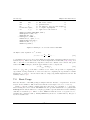
7 MFN: Matrix Function
87
7.1 The Problem f (A)v . . . . . . . . . . . . . . . . . . . . . . . . . . . . . . . . . . 87
7.2 Basic Usage . . . . . . . . . . . . . . . . . . . . . . . . . . . . . . . . . . . . . . . 88
8 Additional Information
8.1 Supported PETSc Features . .
8.2 Supported Matrix Types . . . .
8.3 GPU Computing . . . . . . . .
8.4 Extending SLEPc . . . . . . . .
8.5 Auxiliary Classes . . . . . . . .
8.6 Directory Structure . . . . . . .
8.7 Wrappers to External Libraries
8.8 Fortran Interface . . . . . . . .
.
.
.
.
.
.
.
.
.
.
.
.
.
.
.
.
.
.
.
.
.
.
.
.
.
.
.
.
.
.
.
.
.
.
.
.
.
.
.
.
.
.
.
.
.
.
.
.
.
.
.
.
.
.
.
.
.
.
.
.
.
.
.
.
.
.
.
.
.
.
.
.
.
.
.
.
.
.
.
.
.
.
.
.
.
.
.
.
.
.
.
.
.
.
.
.
.
.
.
.
.
.
.
.
.
.
.
.
.
.
.
.
.
.
.
.
.
.
.
.
.
.
.
.
.
.
.
.
.
.
.
.
.
.
.
.
.
.
.
.
.
.
.
.
.
.
.
.
.
.
.
.
.
.
.
.
.
.
.
.
.
.
.
.
.
.
.
.
.
.
.
.
.
.
.
.
.
.
.
.
.
.
.
.
.
.
.
.
.
.
.
.
.
.
.
.
.
.
.
.
.
.
.
.
.
.
.
.
.
.
.
.
.
.
.
.
.
.
.
.
.
.
.
.
91
91
92
93
94
95
98
99
103
Bibliography
109
Index
113
Chapter
1
Getting Started
slepc, the Scalable Library for Eigenvalue Problem Computations, is a software library for the
solution of large sparse eigenvalue problems on parallel computers.
Together with linear systems of equations, eigenvalue problems are a very important class
of linear algebra problems. The need for the numerical solution of these problems arises in
many situations in science and engineering, in problems associated with stability and vibration
analysis in practical applications. These are usually formulated as large sparse eigenproblems.
Computing eigenvalues is essentially more difficult than solving linear systems of equations.
This has resulted in a very active research activity in the area of computational methods for
eigenvalue problems in the last years, with many remarkable achievements. However, these
state-of-the-art methods and algorithms are not easily transferred to the scientific community,
and, apart from a few exceptions, most user still rely on simpler, well-established techniques.
The reasons for this situation are diverse. First, new methods are increasingly complex and
difficult to implement and therefore robust implementations must be provided by computational
specialists, for example as software libraries. The development of such libraries requires to invest
a lot of effort but sometimes they do not reach normal users due to a lack of awareness.
In the case of eigenproblems, using libraries is not straightforward. It is usually recommended that the user understands how the underlying algorithm works and typically the problem is successfully solved only after several cycles of testing and parameter tuning. Methods
are often specific for a certain class of eigenproblems and this leads to an explosion of available
algorithms from which the user has to choose. Not all these algorithms are available in the form
of software libraries, even less frequently with parallel capabilities.
Another difficulty resides in how to represent the operator matrix. Unlike in dense methods,
there is no widely accepted standard for basic sparse operations in the spirit of blas. This is due
to the fact that sparse storage is more complicated, admitting of more variation, and therefore
1
1.1. SLEPc and PETSc
Chapter 1. Getting Started
less standardized. For this reason, sparse libraries have an added level of complexity. This
holds even more so in the case of parallel distributed-memory programming, where the data of
the problem have to be distributed across the available processors.
The first implementations of algorithms for sparse matrices required a prescribed storage
format for the sparse matrix, which is an obvious limitation. An alternative way of matrix representation is by means of a user-provided subroutine for the matrix-vector product. Apart from
being format-independent, this approach allows the solution of problems in which the matrix
is not available explicitly. The drawback is the restriction to a fixed-prototype subroutine.
A better solution for the matrix representation problem is the well-known reverse communication interface, a technique that allows the development of iterative methods disregarding
the implementation details of various operations. Whenever the iterative method subroutine
needs the results of one of the operations, it returns control to the user’s subroutine that called
it. The user’s subroutine then invokes the module that performs the operation. The iterative
method subroutine is invoked again with the results of the operation.
Several libraries with any of the interface schemes mentioned above are publicly available.
For a survey of such software see the slepc Technical Report [STR-6], “A Survey of Software
for Sparse Eigenvalue Problems”, and references therein. Some of the most recent libraries are
even prepared for parallel execution (some of them can be used from within slepc, see §8.7).
However, they still lack some flexibility or require too much programming effort from the user,
especially in the case that the eigensolution requires to employ advanced techniques such as
spectral transformations or preconditioning.
A further obstacle appears when these libraries have to be used in the context of large
software projects carried out by inter-disciplinary teams. In this scenery, libraries must be able
to interoperate with already existing software and with other libraries. In order to cope with
the complexity associated with such projects, libraries must be designed carefully in order to
overcome hurdles such as different storage formats or programming languages. In the case of
parallel software, care must be taken also to achieve portability to a wide range of platforms
with good performance and still retain flexibility and usability.
1.1
SLEPc and PETSc
The slepc library is an attempt to provide a solution to the situation described in the previous
paragraphs. It is intended to be a general library for the solution of eigenvalue problems that
arise in different contexts, covering standard and generalized problems, both Hermitian and nonHermitian, with either real or complex arithmetic. Issues such as usability, portability, efficiency
and interoperability are addressed, and special emphasis is put on flexibility, providing datastructure neutral implementations and multitude of run-time options. slepc offers a growing
number of eigensolvers as well as interfaces to integrate well-established eigenvalue packages
such as arpack. In addition to the linear eigenvalue problem, slepc also includes other solver
classes for nonlinear eigenproblems, SVD and the computation of the action of a matrix function.
slepc is based on petsc, the Portable, Extensible Toolkit for Scientific Computation [Balay
et al., 2015], and, therefore, a large percentage of the software complexity is avoided since many
—2—
Chapter 1. Getting Started
1.1. SLEPc and PETSc
petsc developments are leveraged, including matrix storage formats and linear solvers, to name
a few. slepc focuses on high level features for eigenproblems, structured around a few object
classes as described below.
petsc uses modern programming paradigms to ease the development of large-scale scientific
application codes in Fortran, C, and C++ and provides a powerful set of tools for the numerical
solution of partial differential equations and related problems on high-performance computers.
Its approach is to encapsulate mathematical algorithms using object-oriented programming
techniques, which allow to manage the complexity of efficient numerical message-passing codes.
All the petsc software is free and used around the world in a variety of application areas.
The design philosophy is not to try to completely conceal parallelism from the application
programmer. Rather, the user initiates a combination of sequential and parallel phases of computations, but the library handles the detailed message passing required during the coordination
of computations. Some of the design principles are described in [Balay et al., 1997].
petsc is built around a variety of data structures and algorithmic objects. The application
programmer works directly with these objects rather than concentrating on the underlying data
structures. Each component manipulates a particular family of objects (for instance, vectors)
and the operations one would like to perform on the objects. The three basic abstract data
objects are index sets, vectors and matrices. Built on top of this foundation are various classes of
solver objects, which encapsulate virtually all information regarding the solution procedure for
a particular class of problems, including the local state and various options such as convergence
tolerances, etc.
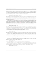
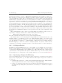
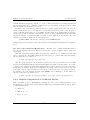
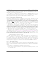
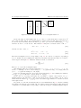
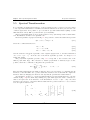
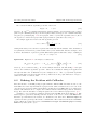
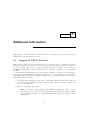
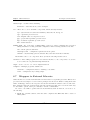
slepc can be considered an extension of petsc providing all the functionality necessary for
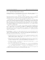
the solution of eigenvalue problems. Figure 1.1 shows a diagram of all the different objects
included in petsc (on the left) and those added by slepc (on the right). petsc is a prerequisite
for slepc and users should be familiar with basic concepts such as vectors and matrices in
order to use slepc. Therefore, together with this manual we recommend to use the petsc
Users Manual [Balay et al., 2015].
Each of these components consists of an abstract interface (simply a set of calling sequences)
and one or more implementations using particular data structures. Both petsc and slepc are
written in C, which lacks direct support for object-oriented programming. However, it is still
possible to take advantage of the three basic principles of object-oriented programming to
manage the complexity of such large packages. petsc uses data encapsulation in both vector
and matrix data objects. Application code accesses data through function calls. Also, all the
operations are supported through polymorphism. The user calls a generic interface routine,
which then selects the underlying routine that handles the particular data structure. Finally,
petsc also uses inheritance in its design. All the objects are derived from an abstract base
object. From this fundamental object, an abstract base object is defined for each petsc object
(Mat, Vec and so on), which in turn has a variety of instantiations that, for example, implement
different matrix storage formats.
petsc/slepc provide clean and effective codes for the various phases of solving PDEs, with
a uniform approach for each class of problems. This design enables easy comparison and use of
different algorithms (for example, to experiment with different Krylov subspace methods, pre-
—3—
1.2. Installation
Chapter 1. Getting Started
PETSc
Nonlinear Systems
Trust
Region
Line
Search
SLEPc
Time Steppers
Other
Polynomial Eigensolver
Backward Pseudo Time
Other
Stepping
Euler
Euler
QLinearTOAR
Arnoldi ization
Nonlinear Eigensolver
SLP
RII
NInterp.
Arnoldi
Krylov Subspace Methods
SVD Solver
M. Function
GMRES CG CGS Bi-CGStab TFQMR Richardson Chebychev Other
Cross Cyclic
Thick R.
Lanczos
Product Matrix
Lanczos
Krylov
Linear Eigensolver
Preconditioners
Additive
Schwarz
Block
Jacobi
Jacobi
ILU
ICC
LU
Other
Krylov-Schur
Block
CSR
Symmetric
Block CSR
Vectors
Standard
Dense
CUSP
Other
Index Sets
CUSP
Indices
JD
LOBPCG
CISS
Other
Spectral Transformation
Matrices
Compressed
Sparse Row
GD
Block
Stride
Shift
BV
Shift-and-invert
Cayley
DS
RG
Preconditioner
FN
Other
Figure 1.1: Numerical components of petsc and slepc.
conditioners, or eigensolvers). Hence, petsc, together with slepc, provide a rich environment
for modeling scientific applications as well as for rapid algorithm design and prototyping.
Options can be specified by means of calls to subroutines in the source code and also as
command-line arguments. Runtime options allow the user to test different tolerances, for example, without having to recompile the program. Also, since petsc provides a uniform interface
to all of its linear solvers —the Conjugate Gradient, GMRES, etc.— and a large family of
preconditioners —block Jacobi, overlapping additive Schwarz, etc.—, one can compare several
combinations of method and preconditioner by simply specifying them at execution time. slepc
shares this good property.
The components enable easy customization and extension of both algorithms and implementations. This approach promotes code reuse and flexibility, and separates the issues of
parallelism from the choice of algorithms. The petsc infrastructure creates a foundation for
building large-scale applications.
1.2
Installation
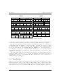
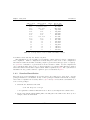
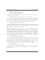
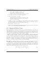
This section describes slepc’s installation procedure. Previously to the installation of slepc,
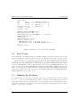
the system must have an appropriate version of petsc installed. Table 1.1 shows a list of slepc
versions and their corresponding petsc versions. slepc versions marked as major releases are
those which incorporate some new functionality. The rest are just adaptations required for a
—4—
Chapter 1. Getting Started
1.2. Installation
slepc version
2.1.0
2.1.1
2.1.5
2.2.0
2.2.1
2.3.0
2.3.1
2.3.2
2.3.3
3.0.0
3.1
3.2
3.3
3.4
3.5
3.6
petsc versions
2.1.0
2.1.1, 2.1.2, 2.1.3
2.1.5, 2.1.6
2.2.0
2.2.1
2.3.0
2.3.1
2.3.1, 2.3.2
2.3.3
3.0.0
3.1
3.2
3.3
3.4
3.5
3.6
Major
?
?
?
?
?
?
?
?
?
?
?
?
?
Release date
Not released
Dec 2002
May 2003
Apr 2004
Aug 2004
Jun 2005
Mar 2006
Oct 2006
Jun 2007
Feb 2009
Aug 2010
Oct 2011
Aug 2012
Jul 2013
Jul 2014
Jun 2015
Table 1.1: Correspondence between slepc and petsc releases.
new petsc release and may also include bug fixes.
The installation process for slepc is very similar to petsc, with two stages: configuration
and compilation. slepc’s configuration is much simpler because most of the configuration
information is taken from petsc, including compiler options and scalar type (real or complex).
See §1.2.2 for a discussion of options that are most relevant for slepc. Several configurations
can coexist in the same directory tree, so that for instance one can have slepc libraries compiled
with real scalars as well as with complex scalars. This is explained in §1.2.3. Also, system-based
installation is also possible with the --prefix option, as discussed in §1.2.4.
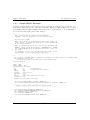
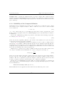
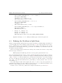
1.2.1
Standard Installation
The basic steps for the installation are described next. Note that prior to these steps, optional
packages must have been installed. If any of these packages is installed afterwards, reconfiguration and recompilation is necessary. Refer to §1.2.2 and §8.7 for details about installation of
some of these packages.
1. Unbundle the distribution file with
$ tar xzf slepc-3.6.0.tar.gz
or an equivalent command. This will create a directory and unpack the software there.
2. Set the environment variable SLEPC_DIR to the full path of the slepc home directory. For
example, under the bash shell:
—5—
1.2. Installation
Chapter 1. Getting Started
$ export SLEPC_DIR=/home/username/slepc-3.6.0
In addition to this variable, PETSC_DIR and PETSC_ARCH must also be set appropriately
(see §1.2.4 for a case in which PETSC_ARCH is not required), for example
$ export PETSC_DIR=/home/username/petsc-3.6.0
$ export PETSC_ARCH=arch-darwin-c-debug
3. Change to the slepc directory and run the configuration script:
$ cd $SLEPC_DIR
$ ./configure
4. If the configuration was successful, build the libraries:
$ make
5. After the compilation, try running some test examples with
$ make test
Examine the output for any obvious errors or problems.
1.2.2
Configuration Options
Several options are available in slepc’s configuration script. To see all available options, type
./configure --help.
In slepc, configure options have the following purposes:
• Specify a directory for prefix-based installation, as explained in §1.2.4.
• Enable external eigensolver packages. For example, to use arpack, specify the following
options (with the appropriate paths):
$ ./configure --with-arpack-dir=/usr/software/ARPACK
--with-arpack-flags=-lparpack,-larpack
Section 8.7 provides more details related to use of external libraries.
Additionally, petsc’s configuration script provides a very long list of options that are relevant
to slepc. Here is a list of options that may be useful. Note that these are options of petsc
that apply to both petsc and slepc, in such a way that it is not possible to, e.g., build petsc
without debugging and slepc with debugging.
• Add --with-scalar-type=complex to build complex scalar versions of all libraries. See
below a note related to complex scalars.
—6—
Chapter 1. Getting Started
1.2. Installation
• Build single precision versions with --with-precision=single. In most applications, this
can achieve a significant reduction of memory requirements, and a moderate reduction of
computing time. Also, quadruple precision (128-bit floating-point representation) is also
available using --with-precision=__float128 on systems with GNU compilers (gcc4.6 or later).
• Enable use from Fortran. By default, petsc’s configure looks for an appropriate Fortran
compiler. If not required, this can be disabled: --with-fortran=0. If required but not
correctly detected, the compiler to be used can be specified with a configure option. In the
case of Fortran 90, additional options are available for building interfaces and datatypes.
• If not detected, use --with-blas-lapack-lib to specify the location of blas and lapack.
If slepc’s configure complains about some missing lapack subroutines, reconfigure petsc
with option --download-f2cblaslapack.
• Enable external libraries that provide direct linear solvers or preconditioners, such as
MUMPS, hypre, or SuperLU; for example, --download-mumps. These are especially relevant for slepc in the case that a spectral transformation is used, see chapter 3.
• Add --with-64-bit-indices=1 to use 8 byte integers (long long) for indexing in vectors
and matrices. This is only needed when working with over roughly 2 billion unknowns.
• Build static libraries, --with-shared-libraries=0. This is generally not recommended,
since shared libraries produce smaller executables and the run time overhead is small.
• Error-checking code can be disabled with --with-debugging=0, but this is only recommended in production runs of well-tested applications.
• Enable GPU computing setting --with-cuda=1 and other options, see §8.3 for details.
Note about complex scalar versions: petsc supports the use of complex scalars by
defining the data type PetscScalar either as a real or complex number. This implies that two
different versions of the petsc libraries can be built separately, one for real numbers and one
for complex numbers, but they cannot be used at the same time. slepc inherits this property.
In slepc it is not possible to completely separate real numbers and complex numbers because
the solution of non-symmetric real-valued eigenvalue problems may be complex. slepc has
been designed trying to provide a uniform interface to manage all the possible cases. However,
there are slight differences between the interface in each of the two versions. In this manual,
differences are clearly identified.
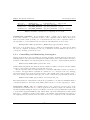
1.2.3
Installing Multiple Configurations in a Single Directory Tree
Often, it is necessary to build two (or more) versions of the libraries that differ in a few configuration options. For instance, versions for real and complex scalars, or versions for double and
single precision, or versions with debugging and optimized. In a standard installation, this is
—7—
1.2. Installation
Chapter 1. Getting Started
handled by building all versions in the same directory tree, as explained below, so that source
code is not replicated unnecessarily. In contrast, in prefix-based installation where source code
is not present, the issue of multiple configurations is handled differently, as explained in §1.2.4.
In a standard installation, the different configurations are identified by a unique name that
is assigned to the environment variable PETSC_ARCH. Let us illustrate how to set up petsc with
two configurations. First, set a value of PETSC_ARCH and proceed with the installation of the
first one:
$
$
$
$
cd $PETSC_DIR
export PETSC_ARCH=arch-linux-gnu-c-debug-real
./configure --with-scalar-type=real
make all test
Note that if PETSC_ARCH is not given a value, petsc suggests one for us. After this, a subdirectory named $PETSC_ARCH is created within $PETSC_DIR, that stores all information associated
with that configuration, including the built libraries, configuration files, automatically generated
source files, and log files. For the second configuration, proceed similarly:
$
$
$
$
cd $PETSC_DIR
export PETSC_ARCH=arch-linux-gnu-c-debug-complex
./configure --with-scalar-type=complex
make all test
The value of PETSC_ARCH in this case must be different than the previous one. It is better to
set the value of PETSC_ARCH explicitly, because the name suggested by configure may coincide
with an existing value, thus overwriting a previous configuration. After successful installation
of the second configuration, two $PETSC_ARCH directories exist within $PETSC_DIR, and the user
can easily choose to build his/her application with either configuration by simply changing the
value of PETSC_ARCH.
The configuration of two versions of slepc in the same directory tree is very similar. The
only important restriction is that the value of PETSC_ARCH used in slepc must exactly match
an existing petsc configuration, that is, a directory $PETSC_DIR/$PETSC_ARCH must exist.
1.2.4
Prefix-based Installation
Both petsc and slepc allow for prefix-based installation. This consists in specifying a directory
to which the files generated during the building process are to be copied.
In petsc, if an installation directory has been specified during configuration (with option
--prefix in step 3 of §1.2.1), then after building the libraries the relevant files are copied to
that directory by typing
$ make install
This is useful for building as a regular user and then copying the libraries and include files to
the system directories as root.
—8—
Chapter 1. Getting Started
1.3. Running SLEPc Programs
To be more precise, suppose that the configuration was done with --prefix=/opt/petsc3.6.0-linux-gnu-c-debug. Then, make install will create directory /opt/petsc-3.6.0linux-gnu-c-debug if it does not exist, and several subdirectories containing the libraries,
the configuration files, and the header files. Note that the source code files are not copied,
nor the documentation, so the size of the installed directory will be much smaller than the
original one. For that reason, it is no longer necessary to allow for several configurations to
share a directory tree. In other words, in a prefix-based installation, variable PETSC_ARCH loses
significance and must be unset. To maintain several configurations, one should specify different
prefix directories, typically with a name that informs about the configuration options used.
In order to prepare a prefix-based installation of slepc that uses a prefix-based installation
of petsc, start by setting the appropriate value of PETSC_DIR. Then, run slepc’s configure with
a prefix directory.
$
$
$
$
$
$
$
export PETSC_DIR=/opt/petsc-3.6.0-linux-gnu-c-debug
unset PETSC_ARCH
cd $SLEPC_DIR
./configure --prefix=/opt/slepc-3.6.0-linux-gnu-c-debug
make
make install
export SLEPC_DIR=/opt/slepc-3.6.0-linux-gnu-c-debug
Note that it is important to unset the value of PETSC_ARCH before slepc’s configure. slepc
will use a temporary arch name during the build (this temporary arch is named installed$PETSC_ARCH, where $PETSC_ARCH is the one used to configure the installed PETSc version). Although it is not a common case, it is also possible to configure slepc without prefix, in which case
the PETSC_ARCH variable must still be empty and the arch directory installed-$PETSC_ARCH is
picked automatically (it is hardwired in file $SLEPC_DIR/lib/slepc/conf/slepcvariables).
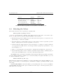
1.3
Running SLEPc Programs
Before using slepc, the user must first set the environment variable SLEPC_DIR, indicating the
full path of the directory containing slepc. For example, under the bash shell, a command of
the form
$ export SLEPC_DIR=/software/slepc-3.6.0
can be placed in the user’s .bashrc file. The SLEPC_DIR directory can be either a standard
installation slepc directory, or a prefix-based installation directory, see §1.2.4. In addition, the
user must set the environment variables required by petsc, that is, PETSC_DIR, to indicate the
full path of the petsc directory, and PETSC_ARCH to specify a particular architecture and set of
options. Note that PETSC_ARCH should not be set in the case of prefix-based installations.
All petsc programs use the MPI (Message Passing Interface) standard for message-passing
communication [MPI Forum, 1994]. Thus, to execute slepc programs, users must know the
procedure for launching MPI jobs on their selected computer system(s). Usually, the mpiexec
command can be used to initiate a program as in the following example that uses eight processes:
—9—
1.4. Writing SLEPc Programs
Chapter 1. Getting Started
$ mpiexec -np 8 slepc_program [command-line options]
Note that MPI may be deactivated during configuration of petsc, if one wants to run only
serial programs in a laptop, for example.
All petsc-compliant programs support the use of the -h or -help option as well as the
-v or -version option. In the case of slepc programs, specific information for slepc is also
displayed.
1.4
Writing SLEPc Programs
Most slepc programs begin with a call to SlepcInitialize
SlepcInitialize(int *argc,char ***argv,char *file,char *help);
which initializes slepc, petsc and MPI. This subroutine is very similar to PetscInitialize, and the arguments have the same meaning. In fact, internally SlepcInitialize calls
PetscInitialize.
After this initialization, slepc programs can use communicators defined by petsc. In most
cases users can employ the communicator PETSC_COMM_WORLD to indicate all processes in a given
run and PETSC_COMM_SELF to indicate a single process. MPI provides routines for generating
new communicators consisting of subsets of processes, though most users rarely need to use
these features. slepc users need not program much message passing directly with MPI, but
they must be familiar with the basic concepts of message passing and distributed memory
computing.
All slepc programs should call SlepcFinalize as their final (or nearly final) statement
ierr = SlepcFinalize();
This routine handles operations to be executed at the conclusion of the program, and calls
PetscFinalize if SlepcInitialize began petsc.
Note to Fortran Programmers: In this manual all the examples and calling sequences
are given for the C/C++ programming languages. However, Fortran programmers can use most
of the functionality of slepc and petsc from Fortran, with only minor differences in the user
interface. For instance, the two functions mentioned above have their corresponding Fortran
equivalent:
call SlepcInitialize(file,ierr)
call SlepcFinalize(ierr)
Section 8.8 provides a summary of the differences between using slepc from Fortran and
C/C++, as well as a complete Fortran example.
— 10 —
Chapter 1. Getting Started
1.4.1
1.4. Writing SLEPc Programs
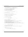
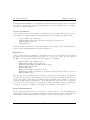
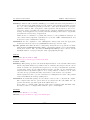
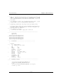
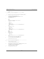
Simple SLEPc Example
A simple example is listed next that solves an eigenvalue problem associated with the onedimensional Laplacian operator discretized with finite differences. This example can be found
in ${SLEPC_DIR}/src/eps/examples/tutorials/ex1.c. Following the code we highlight a
few of the most important parts of this example.
/*
- - - - - - - - - - - - - - - - - - - - - - - - - - - - - - - - - - - - - SLEPc - Scalable Library for Eigenvalue Problem Computations
Copyright (c) 2002-2015, Universitat Politecnica de Valencia, Spain
5
This file is part of SLEPc.
10
SLEPc is free software: you can redistribute it and/or modify it under the
terms of version 3 of the GNU Lesser General Public License as published by
the Free Software Foundation.
15
SLEPc is distributed in the hope that it will be useful, but WITHOUT ANY
WARRANTY; without even the implied warranty of MERCHANTABILITY or FITNESS
FOR A PARTICULAR PURPOSE. See the GNU Lesser General Public License for
more details.
You should have received a copy of the GNU Lesser General Public License
along with SLEPc. If not, see <http://www.gnu.org/licenses/>.
- - - - - - - - - - - - - - - - - - - - - - - - - - - - - - - - - - - - - -
20
*/
static char help[] = "Standard symmetric eigenproblem corresponding to the Laplacian operator in 1 dimension.\n\n"
"The command line options are:\n"
" -n <n>, where <n> = number of grid subdivisions = matrix dimension.\n\n";
25
#include <slepceps.h>
30
35
#undef __FUNCT__
#define __FUNCT__ "main"
int main(int argc,char **argv)
{
Mat
A;
/* problem matrix */
EPS
eps;
/* eigenproblem solver context */
EPSType
type;
PetscReal
error,tol,re,im;
PetscScalar
kr,ki;
Vec
xr,xi;
PetscInt
n=30,i,Istart,Iend,nev,maxit,its,nconv;
PetscErrorCode ierr;
40
SlepcInitialize(&argc,&argv,(char*)0,help);
ierr = PetscOptionsGetInt(NULL,"-n",&n,NULL);CHKERRQ(ierr);
ierr = PetscPrintf(PETSC_COMM_WORLD,"\n1-D Laplacian Eigenproblem, n=%D\n\n",n);CHKERRQ(ierr);
45
/* - - - - - - - - - - - - - - - - - - - - - - - - - - - - - - - - - Compute the operator matrix that defines the eigensystem, Ax=kx
- - - - - - - - - - - - - - - - - - - - - - - - - - - - - - - - - - */
50
ierr
ierr
ierr
ierr
=
=
=
=
MatCreate(PETSC_COMM_WORLD,&A);CHKERRQ(ierr);
MatSetSizes(A,PETSC_DECIDE,PETSC_DECIDE,n,n);CHKERRQ(ierr);
MatSetFromOptions(A);CHKERRQ(ierr);
MatSetUp(A);CHKERRQ(ierr);
55
ierr = MatGetOwnershipRange(A,&Istart,&Iend);CHKERRQ(ierr);
— 11 —
1.4. Writing SLEPc Programs
60
65
Chapter 1. Getting Started
for (i=Istart;i<Iend;i++) {
if (i>0) { ierr = MatSetValue(A,i,i-1,-1.0,INSERT_VALUES);CHKERRQ(ierr); }
if (i<n-1) { ierr = MatSetValue(A,i,i+1,-1.0,INSERT_VALUES);CHKERRQ(ierr); }
ierr = MatSetValue(A,i,i,2.0,INSERT_VALUES);CHKERRQ(ierr);
}
ierr = MatAssemblyBegin(A,MAT_FINAL_ASSEMBLY);CHKERRQ(ierr);
ierr = MatAssemblyEnd(A,MAT_FINAL_ASSEMBLY);CHKERRQ(ierr);
ierr = MatCreateVecs(A,NULL,&xr);CHKERRQ(ierr);
ierr = MatCreateVecs(A,NULL,&xi);CHKERRQ(ierr);
70
/* - - - - - - - - - - - - - - - - - - - - - - - - - - - - - - - - - Create the eigensolver and set various options
- - - - - - - - - - - - - - - - - - - - - - - - - - - - - - - - - - */
/*
Create eigensolver context
*/
ierr = EPSCreate(PETSC_COMM_WORLD,&eps);CHKERRQ(ierr);
75
/*
Set operators. In this case, it is a standard eigenvalue problem
*/
ierr = EPSSetOperators(eps,A,NULL);CHKERRQ(ierr);
ierr = EPSSetProblemType(eps,EPS_HEP);CHKERRQ(ierr);
80
/*
Set solver parameters at runtime
*/
ierr = EPSSetFromOptions(eps);CHKERRQ(ierr);
85
/* - - - - - - - - - - - - - - - - - - - - - - - - - - - - - - - - - Solve the eigensystem
- - - - - - - - - - - - - - - - - - - - - - - - - - - - - - - - - - */
90
95
100
105
110
115
ierr = EPSSolve(eps);CHKERRQ(ierr);
/*
Optional: Get some information from the solver and display it
*/
ierr = EPSGetIterationNumber(eps,&its);CHKERRQ(ierr);
ierr = PetscPrintf(PETSC_COMM_WORLD," Number of iterations of the method: %D\n",its);CHKERRQ(ierr);
ierr = EPSGetType(eps,&type);CHKERRQ(ierr);
ierr = PetscPrintf(PETSC_COMM_WORLD," Solution method: %s\n\n",type);CHKERRQ(ierr);
ierr = EPSGetDimensions(eps,&nev,NULL,NULL);CHKERRQ(ierr);
ierr = PetscPrintf(PETSC_COMM_WORLD," Number of requested eigenvalues: %D\n",nev);CHKERRQ(ierr);
ierr = EPSGetTolerances(eps,&tol,&maxit);CHKERRQ(ierr);
ierr = PetscPrintf(PETSC_COMM_WORLD," Stopping condition: tol=%.4g, maxit=%D\n",(double)tol,maxit);CHKERRQ(ierr);
/* - - - - - - - - - - - - - - - - - - - - - - - - - - - - - - - - - Display solution and clean up
- - - - - - - - - - - - - - - - - - - - - - - - - - - - - - - - - - */
/*
Get number of converged approximate eigenpairs
*/
ierr = EPSGetConverged(eps,&nconv);CHKERRQ(ierr);
ierr = PetscPrintf(PETSC_COMM_WORLD," Number of converged eigenpairs: %D\n\n",nconv);CHKERRQ(ierr);
if (nconv>0) {
/*
Display eigenvalues and relative errors
*/
ierr = PetscPrintf(PETSC_COMM_WORLD,
"
k
||Ax-kx||/||kx||\n"
"
----------------- ------------------\n");CHKERRQ(ierr);
— 12 —
Chapter 1. Getting Started
1.4. Writing SLEPc Programs
for (i=0;i<nconv;i++) {
/*
Get converged eigenpairs: i-th eigenvalue is stored in kr (real part) and
ki (imaginary part)
*/
ierr = EPSGetEigenpair(eps,i,&kr,&ki,xr,xi);CHKERRQ(ierr);
/*
Compute the relative error associated to each eigenpair
*/
ierr = EPSComputeError(eps,i,EPS_ERROR_RELATIVE,&error);CHKERRQ(ierr);
120
125
130
135
140
145
#if defined(PETSC_USE_COMPLEX)
re = PetscRealPart(kr);
im = PetscImaginaryPart(kr);
#else
re = kr;
im = ki;
#endif
if (im!=0.0) {
ierr = PetscPrintf(PETSC_COMM_WORLD," %9f%+9f j %12g\n",(double)re,(double)im,(double)error);CHKERRQ(ierr);
} else {
ierr = PetscPrintf(PETSC_COMM_WORLD,"
%12f
%12g\n",(double)re,(double)error);CHKERRQ(ierr);
}
}
ierr = PetscPrintf(PETSC_COMM_WORLD,"\n");CHKERRQ(ierr);
}
/*
Free work space
*/
ierr = EPSDestroy(&eps);CHKERRQ(ierr);
ierr = MatDestroy(&A);CHKERRQ(ierr);
ierr = VecDestroy(&xr);CHKERRQ(ierr);
ierr = VecDestroy(&xi);CHKERRQ(ierr);
ierr = SlepcFinalize();
return 0;
150
155
}
Include Files
The C/C++ include files for slepc should be used via statements such as
#include <slepceps.h>
where slepceps.h is the include file for the EPS component. Each slepc program must specify
an include file that corresponds to the highest level slepc objects needed within the program;
all of the required lower level include files are automatically included within the higher level
files. For example, slepceps.h includes slepcst.h (spectral transformations), and slepcsys.h
(base slepc file). Some petsc header files are included as well, such as petscksp.h. The slepc
include files are located in the directory ${SLEPC_DIR}/include.
The Options Database
All the petsc functionality related to the options database is available in slepc. This allows the user to input control data at run time very easily. In this example the command
— 13 —
1.4. Writing SLEPc Programs
Chapter 1. Getting Started
PetscOptionsGetInt(NULL,"-n",&n,NULL); checks whether the user has provided a command
line option to set the value of n, the problem dimension. If so, the variable n is set accordingly;
otherwise, n remains unchanged.
Vectors and Matrices
Usage of matrices and vectors in slepc is exactly the same as in petsc. The user can create a
new parallel or sequential matrix, A, which has M global rows and N global columns, with
MatCreate(MPI_Comm comm,Mat *A);
MatSetSizes(Mat A,PetscInt m,PetscInt n,PetscInt M,PetscInt N);
MatSetFromOptions(Mat A);
MatSetUp(Mat A);
where the matrix format can be specified at runtime. The example creates a matrix, sets the
nonzero values with MatSetValues and then assembles it.
Eigensolvers
Usage of eigensolvers is very similar to other kinds of solvers provided by petsc. After creating
the matrix (or matrices) that define the problem, Ax = kx (or Ax = kBx), the user can then
use EPS to solve the system with the following sequence of commands:
EPSCreate(MPI_Comm comm,EPS *eps);
EPSSetOperators(EPS eps,Mat A,Mat B);
EPSSetProblemType(EPS eps,EPSProblemType type);
EPSSetFromOptions(EPS eps);
EPSSolve(EPS eps);
EPSGetConverged(EPS eps,PetscInt *nconv);
EPSGetEigenpair(EPS eps,PetscInt i,PetscScalar *kr,PetscScalar *ki,Vec xr,Vec xi);
EPSDestroy(EPS *eps);
The user first creates the EPS context and sets the operators associated with the eigensystem
as well as the problem type. The user then sets various options for customized solution, solves
the problem, retrieves the solution, and finally destroys the EPS context. Chapter 2 describes
in detail the EPS package, including the options database that enables the user to customize
the solution process at runtime by selecting the solution algorithm and also specifying the
convergence tolerance, the number of eigenvalues, the dimension of the subspace, etc.
Spectral Transformation
In the example program shown above there is no explicit reference to spectral transformations. However, an ST object is handled internally so that the user is able to request different
transformations such as shift-and-invert. Chapter 3 describes the ST package in detail.
— 14 —
Chapter 1. Getting Started
1.4. Writing SLEPc Programs
Error Checking
All slepc routines return an integer indicating whether an error has occurred during the call.
The error code is set to be nonzero if an error has been detected; otherwise, it is zero. The
petsc macro CHKERRQ(ierr) checks the value of ierr and calls the petsc error handler upon
error detection. CHKERRQ(ierr) should be placed after all subroutine calls to enable a complete
error traceback. See the petsc documentation for full details.
1.4.2
Writing Application Codes with SLEPc
Several example programs demonstrate the software usage and can serve as templates for developing custom applications. They are scattered throughout the SLEPc directory tree, in
particular in the examples/tutorials directories under each class subdirectory.
To write a new application program using slepc, we suggest the following procedure:
1. Install and test slepc according to the instructions given in the documentation.
2. Copy the slepc example that corresponds to the class of problem of interest (e.g., singular
value decomposition).
3. Copy the makefile within the example directory (or create a new one as explained below);
compile and run the example program.
4. Use the example program as a starting point for developing a custom code.
Application program makefiles can be set up very easily just by including one file from
the slepc makefile system. All the necessary petsc definitions are loaded automatically. The
following sample makefile illustrates how to build C and Fortran programs:
default: ex1
include ${SLEPC_DIR}/lib/slepc/conf/slepc_common
5
10
ex1: ex1.o chkopts
-${CLINKER} -o ex1 ex1.o ${SLEPC_EPS_LIB}
${RM} ex1.o
ex1f: ex1f.o chkopts
-${FLINKER} -o ex1f ex1f.o ${SLEPC_EPS_LIB}
${RM} ex1f.o
— 15 —
1.4. Writing SLEPc Programs
Chapter 1. Getting Started
— 16 —
Chapter
2
EPS: Eigenvalue Problem Solver
The Eigenvalue Problem Solver (EPS) is the main object provided by slepc. It is used to specify
a linear eigenvalue problem, either in standard or generalized form, and provides uniform and
efficient access to all of the linear eigensolvers included in the package. Conceptually, the level
of abstraction occupied by EPS is similar to other solvers in petsc such as KSP for solving linear
systems of equations.
2.1
Eigenvalue Problems
In this section, we briefly present some basic concepts about eigenvalue problems as well as
general techniques used to solve them. The description is not intended to be exhaustive. The
objective is simply to define terms that will be referred to throughout the rest of the manual.
Readers who are familiar with the terminology and the solution approach can skip this section.
For a more comprehensive description, we refer the reader to monographs such as [Stewart,
2001], [Bai et al., 2000], [Saad, 1992] or [Parlett, 1980]. A historical perspective of the topic
can be found in [Golub and van der Vorst, 2000]. See also the slepc technical reports.
In the standard formulation, the linear eigenvalue problem consists in the determination of
λ ∈ C for which the equation
Ax = λx
(2.1)
has nontrivial solution, where A ∈ Cn×n and x ∈ Cn . The scalar λ and the vector x are called
eigenvalue and (right) eigenvector, respectively. Note that they can be complex even when the
matrix is real. If λ is an eigenvalue of A then λ̄ is an eigenvalue of its conjugate transpose, A∗ ,
or equivalently
y ∗A = λ y ∗ ,
(2.2)
17
2.1. Eigenvalue Problems
Chapter 2. EPS: Eigenvalue Problem Solver
where y is called the left eigenvector.
In many applications, the problem is formulated as
Ax = λBx,
(2.3)
where B ∈ Cn×n , which is known as the generalized eigenvalue problem. Usually, this problem
is solved by reformulating it in standard form, for example B −1 Ax = λx if B is non-singular.
slepc focuses on the solution of problems in which the matrices are large and sparse. Hence,
only methods that preserve sparsity are considered. These methods obtain the solution from the
information generated by the application of the operator to various vectors (the operator is a
simple function of matrices A and B), that is, matrices are only used in matrix-vector products.
This not only maintains sparsity but allows the solution of problems in which matrices are not
available explicitly.
In practical analyses, from the n possible solutions, typically only a few eigenpairs (λ, x) are
considered relevant, either in the extremities of the spectrum, in an interval, or in a region of
the complex plane. Depending on the application, either eigenvalues or eigenvectors (or both)
are required. In some cases, left eigenvectors are also of interest.
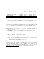
Projection Methods. Most eigensolvers provided by slepc perform a Rayleigh-Ritz projection for extracting the spectral approximations, that is, they project the problem onto a
low-dimensional subspace that is built appropriately. Suppose that an orthogonal basis of this
subspace is given by Vj = [v1 , v2 , . . . , vj ]. If the solutions of the projected (reduced) problem
Bj s = θs (i.e., VjT AVj = Bj ) are assumed to be (θi , si ), i = 1, 2, . . . , j, then the approximate
eigenpairs (λ̃i , x̃i ) of the original problem (Ritz value and Ritz vector) are obtained as
λ̃i = θi ,
(2.4)
x̃i = Vj si .
(2.5)
Starting from this general idea, eigensolvers differ from each other in which subspace is used,
how it is built and other technicalities aimed at improving convergence, reducing storage requirements, etc.
The subspace
Km (A, v) ≡ span v, Av, A2 v, . . . , Am−1 v ,
(2.6)
is called the m-th Krylov subspace corresponding to A and v. Methods that use subspaces of
this kind to carry out the projection are called Krylov methods. One example of such methods
is the Arnoldi algorithm: starting with v1 , kv1 k2 = 1, the Arnoldi basis generation process can
be expressed by the recurrence
vj+1 hj+1,j = wj = Avj −
j
X
hi,j vi ,
(2.7)
i=1
where hi,j are the scalar coefficients obtained in the Gram-Schmidt orthogonalization of Avj
with respect to vi , i = 1, 2, . . . , j, and hj+1,j = kwj k2 . Then, the columns of Vj span the Krylov
— 18 —
Chapter 2. EPS: Eigenvalue Problem Solver
2.1. Eigenvalue Problems
subspace Kj (A, v1 ) and Ax = λx is projected into Hj s = θs, where Hj is an upper Hessenberg
matrix with elements hi,j , which are 0 for i ≥ j + 2. The related Lanczos algorithms obtain a
projected matrix that is tridiagonal.
A generalization to the above methods are the block Krylov strategies, in which the starting
vector v1 is replaced by a full rank n×p matrix V1 , which allows for better convergence properties
when there are multiple eigenvalues and can provide better data management on some computer
architectures. Block tridiagonal and block Hessenberg matrices are then obtained as projections.
It is generally assumed (and observed) that the Lanczos and Arnoldi algorithms find solutions at the extremities of the spectrum. Their convergence pattern, however, is strongly
related to the eigenvalue distribution. Slow convergence may be experienced in the presence
of tightly clustered eigenvalues. The maximum allowable j may be reached without having
achieved convergence for all desired solutions. Then, restarting is usually a useful technique
and different strategies exist for that purpose. However, convergence can still be very slow
and acceleration strategies must be applied. Usually, these techniques consist in computing
eigenpairs of a transformed operator and then recovering the solution of the original problem.
The aim of these transformations is twofold. On one hand, they make it possible to obtain
eigenvalues other than those lying in the boundary of the spectrum. On the other hand, the
separation of the eigenvalues of interest is improved in the transformed spectrum thus leading to
faster convergence. The most commonly used spectral transformation is called shift-and-invert,
which works with operator (A − σI)−1 . It allows the computation of eigenvalues closest to σ
with very good separation properties. When using this approach, a linear system of equations,
(A − σI)y = x, must be solved in each iteration of the eigenvalue process.
Preconditioned Eigensolvers. In many applications, Krylov eigensolvers perform very well
because Krylov subspaces are optimal in a certain theoretical sense. However, these methods
may not be appropriate in some situations such as the computation of interior eigenvalues.
The spectral transformation mentioned above may not be a viable solution or it may be too
costly. For these reasons, other types of eigensolvers such as Davidson and Jacobi-Davidson rely
on a different way of expanding the subspace. Instead of satisfying the Krylov relation, these
methods compute the new basis vector by the so-called correction equation. The resulting
subspace may be richer in the direction of the desired eigenvectors. These solvers may be
competitive especially for computing interior eigenvalues. From a practical point of view, the
correction equation may be seen as a cheap replacement for the shift-and-invert system of
equations, (A − σI)y = x. By cheap we mean that it may be solved inaccurately without
compromising robustness, via a preconditioned iterative linear solver. For this reason, these are
known as preconditioned eigensolvers.
Related Problems. In many applications such as the analysis of damped vibrating systems
the problem to be solved is a polynomial eigenvalue problem (PEP), or more generally a nonlinear eigenvalue problem (NEP). For these, the reader is referred to chapters 5 and 6. Another
linear algebra problem that is very closely related to the eigenvalue problem is the singular
value decomposition (SVD), see chapter 4.
— 19 —
2.2. Basic Usage
5
10
15
Chapter 2. EPS: Eigenvalue Problem Solver
EPS
Mat
Vec
PetscScalar
PetscInt
PetscReal
eps;
A;
xr, xi;
kr, ki;
j, nconv;
error;
/*
/*
/*
/*
eigensolver context
matrix of Ax=kx
eigenvector, x
eigenvalue, k
*/
*/
*/
*/
EPSCreate( PETSC_COMM_WORLD, &eps );
EPSSetOperators( eps, A, NULL );
EPSSetProblemType( eps, EPS_NHEP );
EPSSetFromOptions( eps );
EPSSolve( eps );
EPSGetConverged( eps, &nconv );
for (j=0; j<nconv; j++) {
EPSGetEigenpair( eps, j, &kr, &ki, xr, xi );
EPSComputeError( eps, j, EPS_ERROR_RELATIVE, &error );
}
EPSDestroy( &eps );
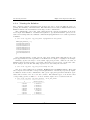
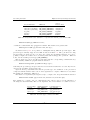
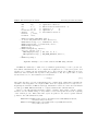
Figure 2.1: Example code for basic solution with EPS.
2.2
Basic Usage
The EPS module in slepc is used in a similar way as petsc modules such as KSP. All the
information related to an eigenvalue problem is handled via a context variable. The usual object
management functions are available (EPSCreate, EPSDestroy, EPSView, EPSSetFromOptions).
In addition, the EPS object provides functions for setting several parameters such as the number
of eigenvalues to compute, the dimension of the subspace, the portion of the spectrum of interest,
the requested tolerance or the maximum number of iterations allowed.
The solution of the problem is obtained in several steps. First of all, the matrices associated
with the eigenproblem are specified via EPSSetOperators and EPSSetProblemType is used to
specify the type of problem. Then, a call to EPSSolve is done that invokes the subroutine for
the selected eigensolver. EPSGetConverged can be used afterwards to determine how many of
the requested eigenpairs have converged to working accuracy. EPSGetEigenpair is finally used
to retrieve the eigenvalues and eigenvectors.
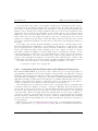
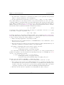
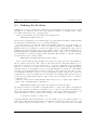
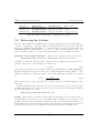
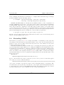
In order to illustrate the basic functionality of the EPS package, a simple example is shown in
Figure 2.1. The example code implements the solution of a simple standard eigenvalue problem.
Code for setting up the matrix A is not shown and error-checking code is omitted.
All the operations of the program are done over a single EPS object. This solver context is
created in line 8 with the command
EPSCreate(MPI_Comm comm,EPS *eps);
Here comm is the MPI communicator, and eps is the newly formed solver context. The com-
— 20 —
Chapter 2. EPS: Eigenvalue Problem Solver
2.2. Basic Usage
municator indicates which processes are involved in the EPS object. Most of the EPS operations
are collective, meaning that all the processes collaborate to perform the operation in parallel.
Before actually solving an eigenvalue problem with EPS, the user must specify the matrices
associated with the problem, as in line 9, with the following routine
EPSSetOperators(EPS eps,Mat A,Mat B);
The example specifies a standard eigenproblem. In the case of a generalized problem, it would
be necessary also to provide matrix B as the third argument to the call. The matrices specified
in this call can be in any petsc format. In particular, EPS allows the user to solve matrix-free
problems by specifying matrices created via MatCreateShell. A more detailed discussion of
this issue is given in §8.2.
After setting the problem matrices, the problem type is set with EPSSetProblemType. This
is not strictly necessary since if this step is skipped then the problem type is assumed to be
non-symmetric. More details are given in §2.3. At this point, the value of the different options
could optionally be set by means of a function call such as EPSSetTolerances (explained later
in this chapter). After this, a call to EPSSetFromOptions should be made as in line 11,
EPSSetFromOptions(EPS eps);
The effect of this call is that options specified at runtime in the command line are passed
to the EPS object appropriately. In this way, the user can easily experiment with different
combinations of options without having to recompile. All the available options as well as the
associated function calls are described later in this chapter.
Line 12 launches the solution algorithm, simply with the command
EPSSolve(EPS eps);
The subroutine that is actually invoked depends on which solver has been selected by the user.
After the call to EPSSolve has finished, all the data associated with the solution of the
eigenproblem is kept internally. This information can be retrieved with different function calls,
as in lines 13 to 17. This part is described in detail in §2.5.
Once the EPS context is no longer needed, it should be destroyed with the command
EPSDestroy(EPS *eps);
The above procedure is sufficient for general use of the EPS package. As in the case of the
KSP solver, the user can optionally explicitly call
EPSSetUp(EPS eps);
before calling EPSSolve to perform any setup required for the eigensolver.
Internally, the EPS object works with an ST object (spectral transformation, described in
chapter 3). To allow application programmers to set any of the spectral transformation options
directly within the code, the following routine is provided to extract the ST context,
EPSGetST(EPS eps,ST *st);
— 21 —
2.3. Defining the Problem
Chapter 2. EPS: Eigenvalue Problem Solver
Problem Type
Hermitian
Non-Hermitian
Generalized Hermitian
Generalized Hermitian indefinite
Generalized Non-Hermitian
GNHEP with positive (semi-)definite B
EPSProblemType
EPS_HEP
EPS_NHEP
EPS_GHEP
EPS_GHIEP
EPS_GNHEP
EPS_PGNHEP
Command line key
-eps_hermitian
-eps_non_hermitian
-eps_gen_hermitian
-eps_gen_indefinite
-eps_gen_non_hermitian
-eps_pos_gen_non_hermitian
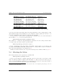
Table 2.1: Problem types considered in EPS.
With the command
EPSView(EPS eps,PetscViewer viewer);
it is possible to examine the actual values of the different settings of the EPS object, including
also those related to the associated ST object. This is useful for making sure that the solver is
using the settings that the user wants.
2.3
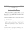
Defining the Problem
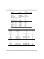
slepc is able to cope with different kinds of problems. Currently supported problem types
are listed in Table 2.1. An eigenproblem is generalized (Ax = λBx) if the user has specified
two matrices (see EPSSetOperators above), otherwise it is standard (Ax = λx). A standard
eigenproblem is Hermitian if matrix A is Hermitian (i.e., A = A∗ ) or, equivalently in the
case of real matrices, if matrix A is symmetric (i.e., A = AT ). A generalized eigenproblem is
Hermitian if matrix A is Hermitian (symmetric) and B is Hermitian (symmetric) and positive
(semi-)definite. If B is not positive (semi-)definite then the problem cannot be considered
Hermitian but symmetry can still be exploited to some extent in some solvers (problem type
EPS_GHIEP). A special case of generalized non-Hermitian problem is when A is non-Hermitian
but B is Hermitian and positive (semi-)definite, see §3.4.3 and §3.4.4 for discussion.
The problem type can be specified at run time with the corresponding command line key
or, more usually, within the program with the function
EPSSetProblemType(EPS eps,EPSProblemType type);
By default, slepc assumes that the problem is non-Hermitian. Some eigensolvers are able
to exploit symmetry, that is, they compute a solution for Hermitian problems with less storage and/or computational cost than other methods that ignore this property. Also, symmetric
solvers may be more accurate. On the other hand, some eigensolvers in slepc only have a
symmetric version and will abort if the problem is non-Hermitian. In the case of generalized
eigenproblems some considerations apply regarding symmetry, especially in the case of singular B. This topic is tackled in §3.4.3 and §3.4.4. For all these reasons, the user is strongly
recommended to always specify the problem type in the source code.
The type of the problem can be determined with the functions
— 22 —
Chapter 2. EPS: Eigenvalue Problem Solver
2.3. Defining the Problem
EPSIsGeneralized(EPS eps,PetscBool *gen);
EPSIsHermitian(EPS eps,PetscBool *her);
EPSIsPositive(EPS eps,PetscBool *pos);
The user can specify how many eigenvalues (and eigenvectors) to compute. The default is
to compute only one. The function
EPSSetDimensions(EPS eps,PetscInt nev,PetscInt ncv,PetscInt mpd);
allows the specification of the number of eigenvalues to compute, nev. The second argument
can be set to prescribe the number of column vectors to be used by the solution algorithm, ncv,
that is, the largest dimension of the working subspace. The third argument has to do with a
more advanced usage, as explained in §2.6.5. These parameters can also be set at run time with
the options -eps_nev, -eps_ncv and -eps_mpd. For example, the command line
$ ./program -eps_nev 10 -eps_ncv 24
requests 10 eigenvalues and instructs to use 24 column vectors. Note that ncv must be at least
equal to nev, although in general it is recommended (depending on the method) to work with
a larger subspace, for instance ncv ≥ 2 · nev or even more. The case that the user requests a
relatively large number of eigenpairs is discussed in §2.6.5.
Eigenvalues of Interest. For the selection of the portion of the spectrum of interest, there
are several alternatives. In real symmetric problems, one may want to compute the largest or
smallest eigenvalues in magnitude, or the leftmost or rightmost ones, or even all eigenvalues
in a given interval. In other problems, in which the eigenvalues can be complex, then one can
select eigenvalues depending on the magnitude, or the real part or even the imaginary part.
Sometimes the eigenvalues of interest are those closest to a given target value, τ , measuring the
distance either in the ordinary way or along the real (or imaginary) axis. In some other cases,
wanted eigenvalues must be found in a given region of the complex plane. Table 2.2 summarizes
all the possibilities available for the function
EPSSetWhichEigenpairs(EPS eps,EPSWhich which);
which can also be specified at the command line. This criterion is used both for configuring
how the eigensolver seeks eigenvalues (note that not all these possibilities are available for all
the solvers) and also for sorting the computed values. The default is to compute the largest
magnitude eigenvalues, except for those solvers in which this option is not available. There is
another exception related to the use of some spectral transformations, see chapter 3.
For the sorting criteria relative to a target value, the following function must be called in
order to specify such value τ :
EPSSetTarget(EPS eps,PetscScalar target);
or, alternatively, with the command-line key -eps_target. Note that, since the target is defined
as a PetscScalar, complex values of τ are allowed only in the case of complex scalar builds of
the SLEPc library.
— 23 —
2.3. Defining the Problem
EPSWhich
EPS_LARGEST_MAGNITUDE
EPS_SMALLEST_MAGNITUDE
EPS_LARGEST_REAL
EPS_SMALLEST_REAL
EPS_LARGEST_IMAGINARY
EPS_SMALLEST_IMAGINARY
EPS_TARGET_MAGNITUDE
EPS_TARGET_REAL
EPS_TARGET_IMAGINARY
EPS_ALL
EPS_WHICH_USER
Chapter 2. EPS: Eigenvalue Problem Solver
Command line key
-eps_largest_magnitude
-eps_smallest_magnitude
-eps_largest_real
-eps_smallest_real
-eps_largest_imaginary
-eps_smallest_imaginary
-eps_target_magnitude
-eps_target_real
-eps_target_imaginary
-eps_all
Sorting criterion
Largest |λ|
Smallest |λ|
Largest Re(λ)
Smallest Re(λ)
Largest Im(λ)1
Smallest Im(λ)1
Smallest |λ − τ |
Smallest |Re(λ − τ )|
Smallest |Im(λ − τ )|
All λ ∈ [a, b]
user-defined
Table 2.2: Available possibilities for selection of the eigenvalues of interest.
The use of a target value makes sense if the eigenvalues of interest are located in the interior
of the spectrum. Since these eigenvalues are usually more difficult to compute, the eigensolver
by itself may not be able to obtain them, and additional tools are normally required. There are
two possibilities for this:
• To use harmonic extraction (see §2.6.6), a variant of some solvers that allows a better
approximation of interior eigenvalues without changing the way the subspace is built.
• To use a spectral transformation such as shift-and-invert (see chapter 3), where the subspace is built from a transformed problem (usually much more costly).
The special case of computing all eigenvalues in an interval is discussed in §3.4.5, since it is
related also to spectral transformations. In this case, instead of a target value the user has to
specify the computational interval with
EPSSetInterval(EPS eps,PetscScalar a,PetscScalar b);
which is equivalent to -eps_interval <a,b>.
There is also support for specifying a region of the complex plane so that the eigensolver
finds eigenvalues within that region only. This possibility is described in §2.6.4.
Finally, we mention the possibility of defining an arbitrary sorting criterion by means of
EPS_WHICH_USER in combination with EPSSetEigenvalueComparison.
The selection criteria discussed above are based solely on the eigenvalue. In some special situations, it is necessary to establish a user-defined criterion that also makes use of the eigenvector
when deciding which are the most wanted eigenpairs. For these cases, use EPSSetArbitrarySelection.
1 If slepc is compiled for real scalars, then the absolute value of the imaginary part, |Im(λ)|, is used for
eigenvalue selection and sorting.
— 24 —
Chapter 2. EPS: Eigenvalue Problem Solver
2.4
2.4. Selecting the Eigensolver
Selecting the Eigensolver
The available methods for solving the eigenvalue problems are the following:
• Basic methods
– Power Iteration with deflation. When combined with shift-and-invert (see chapter
3), it is equivalent to the Inverse Iteration. Also, this solver embeds the Rayleigh
Quotient Iteration (RQI) by allowing variable shifts.
– Subspace Iteration with Rayleigh-Ritz projection and locking.
– Arnoldi method with explicit restart and deflation.
– Lanczos with explicit restart, deflation, and different reorthogonalization strategies.
• Krylov-Schur, a variation of Arnoldi with a very effective restarting technique. In the case
of symmetric problems, this is equivalent to the thick-restart Lanczos method.
• Generalized Davidson, a simple iteration based on the subspace expansion by the preconditioned residual.
• Jacobi-Davidson, a preconditioned eigensolver with an effective correction equation.
• RQCG, a basic conjugate gradient iteration for the minimization of the Rayleigh quotient.
• LOBPCG, the locally-optimal block preconditioned conjugate gradient.
• CISS, a contour-integral solver that allows computing all eigenvalues in a given region.
The default solver is Krylov-Schur. A detailed description of the implemented algorithms
is provided in the slepc Technical Reports. In addition to these methods, slepc also provides
wrappers to external packages such as arpack, blzpack, or trlan. A complete list of these
interfaces can be found in §8.7.
As an alternative, slepc provides an interface to some lapack routines. These routines
operate in dense mode with only one processor and therefore are suitable only for moderate
size problems. This solver should be used only for debugging purposes.
The solution method can be specified procedurally or via the command line. The application
programmer can set it by means of the command
EPSSetType(EPS eps,EPSType method);
while the user writes the options database command -eps_type followed by the name of the
method (see Table 2.3).
Not all the methods can be used for all problem types. Table 2.4 summarizes the scope of
each eigensolver by listing which portion of the spectrum can be selected (as defined in Table
2.2), which problem types are supported (as defined in Table 2.1) and whether they are available
or not in the complex version of slepc.
— 25 —
2.4. Selecting the Eigensolver
Chapter 2. EPS: Eigenvalue Problem Solver
Method
Power / Inverse / RQI
Subspace Iteration
Arnoldi
Lanczos
Krylov-Schur
Generalized Davidson
Jacobi-Davidson
Rayleigh quotient CG
LOBPCG
Contour integral SS
lapack solver
Wrapper to arpack
Wrapper to primme
Wrapper to blzpack
Wrapper to trlan
Wrapper to blopex
Wrapper to feast
EPSType
EPSPOWER
EPSSUBSPACE
EPSARNOLDI
EPSLANCZOS
EPSKRYLOVSCHUR
EPSGD
EPSJD
EPSRQCG
EPSLOBPCG
EPSCISS
EPSLAPACK
EPSARPACK
EPSPRIMME
EPSBLZPACK
EPSTRLAN
EPSBLOPEX
EPSFEAST
Options
Database Name
power
subspace
arnoldi
lanczos
krylovschur
gd
jd
rqcg
lobpcg
ciss
lapack
arpack
primme
blzpack
trlan
blopex
feast
Default
?
Table 2.3: Eigenvalue solvers available in the EPS module.
Method
power
subspace
arnoldi
lanczos
krylovschur
gd
jd
rqcg
lobpcg
ciss
lapack
arpack
primme
blzpack
trlan
blopex
feast
Portion of spectrum
Largest |λ|
Largest |λ|
any
any
any
any
any
Smallest Re(λ)
Smallest Re(λ)
All λ in region
any
any
Largest and smallest Re(λ)
Smallest Re(λ)
Largest and smallest Re(λ)
Smallest Re(λ)
All λ in an interval
Problem type
any
any
any
EPS_HEP, EPS_GHEP
any
any
any
EPS_HEP, EPS_GHEP
EPS_HEP, EPS_GHEP
any
any
any
EPS_HEP
EPS_HEP, EPS_GHEP
EPS_HEP
EPS_HEP, EPS_GHEP
EPS_HEP, EPS_GHEP
Real/Complex
both
both
both
both
both
both
both
both
both
both
both
both
both
real
real
both
complex
Table 2.4: Supported problem types for all eigensolvers available in slepc.
— 26 —
Chapter 2. EPS: Eigenvalue Problem Solver
2.5
2.5. Retrieving the Solution
Retrieving the Solution
Once the call to EPSSolve is complete, all the data associated with the solution of the eigenproblem is kept internally in the EPS object. This information can be obtained by the calling
program by means of a set of functions described in this section.
As explained below, the number of computed solutions depends on the convergence and,
therefore, it may be different from the number of solutions requested by the user. So the first
task is to find out how many solutions are available, with
EPSGetConverged(EPS eps,PetscInt *nconv);
Usually, the number of converged solutions, nconv, will be equal to nev, but in general it
will be a number ranging from 0 to ncv (here, nev and ncv are the arguments of function
EPSSetDimensions).
2.5.1
The Computed Solution
The user may be interested in the eigenvalues, or the eigenvectors, or both. The function
EPSGetEigenpair(EPS eps,PetscInt j,PetscScalar *kr,PetscScalar *ki,
Vec xr,Vec xi);
returns the j-th computed eigenvalue/eigenvector pair. Typically, this function is called inside
a loop for each value of j from 0 to nconv–1. Note that eigenvalues are ordered according to
the same criterion specified with function EPSSetWhichEigenpairs for selecting the portion of
the spectrum of interest. The meaning of the last 4 parameters depends on whether slepc has
been compiled for real or complex scalars, as detailed below. The eigenvectors are normalized
so that they have a unit 2-norm, except for problem type EPS_GHEP in which case returned
eigenvectors have a unit B-norm.
Real slepc. In this case, all Mat and Vec objects are real. The computed approximate solution
returned by the function EPSGetEigenpair is stored in the following way: kr and ki contain the
real and imaginary parts of the eigenvalue, respectively, and xr and xi contain the associated
eigenvector. Two cases can be distinguished:
• When ki is zero, it means that the j-th eigenvalue is a real number. In this case, kr is
the eigenvalue and xr is the corresponding eigenvector. The vector xi is set to all zeros.
• If ki is different from zero, then the j-th eigenvalue is a complex number and, therefore, it
is part of a complex conjugate pair. Thus, the j-th eigenvalue is kr+ i·ki. With respect to
the eigenvector, xr stores the real part of the eigenvector and xi the imaginary part, that
is, the j-th eigenvector is xr+ i·xi. The (j + 1)-th eigenvalue (and eigenvector) will be the
corresponding complex conjugate and will be returned when function EPSGetEigenpair
is invoked with index j+1. Note that the sign of the imaginary part is returned correctly
in all cases (users need not change signs).
— 27 —
2.5. Retrieving the Solution
Chapter 2. EPS: Eigenvalue Problem Solver
Complex slepc. In this case, all Mat and Vec objects are complex. The computed solution
returned by function EPSGetEigenpair is the following: kr contains the (complex) eigenvalue
and xr contains the corresponding (complex) eigenvector. In this case, ki and xi are not used
(set to all zeros).
2.5.2
Reliability of the Computed Solution
In this subsection, we discuss how a-posteriori error bounds can be obtained in order to assess
the accuracy of the computed solutions. These bounds are based on the so-called residual
vector, defined as
r = Ax̃ − λ̃x̃,
(2.8)
or r = Ax̃ − λ̃B x̃ in the case of a generalized problem, where λ̃ and x̃ represent any of the
nconv computed eigenpairs delivered by EPSGetEigenpair (note that this function returns a
normalized x̃).
In the case of Hermitian problems, it is possible to demonstrate the following property (see
for example [Saad, 1992, ch. 3]):
|λ − λ̃| ≤ krk2 ,
(2.9)
where λ is an exact eigenvalue. Therefore, the 2-norm of the residual vector can be used as a
bound for the absolute error in the eigenvalue.
In the case of non-Hermitian problems, the situation is worse because no simple relation
such as Eq. 2.9 is available. This means that in this case the residual norms may still give
an indication of the actual error but the user should be aware that they may sometimes be
completely wrong, especially in the case of highly non-normal matrices. A better bound would
involve also the residual norm of the left eigenvector.
With respect to eigenvectors, we have a similar scenario in the sense that bounds for the
error may be established in the Hermitian case only, for example the following one:
sin θ(x, x̃) ≤
krk2
,
δ
(2.10)
where θ(x, x̃) is the angle between the computed and exact eigenvectors, and δ is the distance
from λ̃ to the rest of the spectrum. This bound is not provided by slepc because δ is not
available. The above expression is given here simply to warn the user about the fact that
accuracy of eigenvectors may be deficient in the case of clustered eigenvalues.
In the case of non-Hermitian problems, slepc provides the alternative of retrieving an
orthonormal basis of an invariant subspace instead of getting individual eigenvectors. This
is done with function
EPSGetInvariantSubspace(EPS eps,Vec *v);
This is sufficient in some applications and is safer from the numerical point of view.
— 28 —
Chapter 2. EPS: Eigenvalue Problem Solver
Error type
Absolute error
Relative error
Backward error
EPSErrorType
EPS_ERROR_ABSOLUTE
EPS_ERROR_RELATIVE
EPS_ERROR_BACKWARD
2.5. Retrieving the Solution
Command line key
-eps_error_absolute
-eps_error_relative
-eps_error_backward
Error bound
krk
krk/|λ|
krk/(kAk + |λ|kBk)
Table 2.5: Available expressions for computing error bounds.
Computation of Bounds. It is sometimes useful to compute error bounds based on the
norm of the residual rj , to assess the accuracy of the computed solution. The bound can be
made in absolute terms, as in Eq. 2.9, or alternatively the error can be expressed relative to
the eigenvalue or to the matrix norms. For this, the following function can be used:
EPSComputeError(EPS eps,PetscInt j,EPSErrorType type,PetscReal *error);
The types of errors that can be computed are summarized in Table 2.5. The way in which
the error is computed is unrelated to the error estimation used internally in the solver for
convergence checking, as described below.
2.5.3
Controlling and Monitoring Convergence
All the eigensolvers provided by slepc are iterative in nature, meaning that the solutions are
(usually) improved at each iteration until they are sufficiently accurate, that is, until convergence
is achieved. The number of iterations required by the process can be obtained with the function
EPSGetIterationNumber(EPS eps,PetscInt *its);
which returns in argument its either the iteration number at which convergence was successfully
reached, or the iteration at which a problem was detected.
The user specifies when a solution should be considered sufficiently accurate by means of
a tolerance. An approximate eigenvalue is considered to be converged if the error estimate
associated with it is below the specified tolerance. The default value of the tolerance is 10−8
and can be changed at run time with -eps_tol <tol> or inside the program with the function
EPSSetTolerances(EPS eps,PetscReal tol,PetscInt max_it);
The third parameter of this function allows the programmer to modify the maximum number
of iterations allowed to the solution algorithm, which can also be set via -eps_max_it <its>.
Convergence Check. The error estimates used for the convergence test are based on the
residual norm, as discussed in §2.5.2. Most eigensolvers explicitly compute the residual of the
relevant eigenpairs during the iteration, but Krylov solvers use a cheap formula instead, allowing
to track many eigenpairs simultaneously. When using a spectral transformation, this formula
may give too optimistic bounds (corresponding to the residual of the transformed problem, not
the original problem). In such cases, the users can force the computation of the residual with
— 29 —
2.5. Retrieving the Solution
Chapter 2. EPS: Eigenvalue Problem Solver
Convergence criterion
Absolute
Relative to eigenvalue
Relative to matrix norms
User-defined
EPSConv
EPS_CONV_ABS
EPS_CONV_EIG
EPS_CONV_NORM
EPS_USER
Command line key
-eps_conv_abs
-eps_conv_eig
-eps_conv_norm
-eps_conv_user
Error bound
krk
krk/|λ|
krk/(kAk + |λ|kBk)
user function
Table 2.6: Available possibilities for the convergence criterion.
EPSSetTrueResidual(EPS eps,PetscBool trueres);
or with -eps_true_residual.
From the residual norm, the error bound can be computed in different ways, see Table 2.6.
This can be set via the corresponding command-line switch or with
EPSSetConvergenceTest(EPS eps,EPSConv conv);
The default is to use the criterion relative to the eigenvalue (note: for computing eigenvalues
close to the origin this criterion will likely give very poor accuracy, so the user is advised to
use EPS_CONV_ABS in that case). Finally, a custom convergence criterion may be established by
specifying a user function (EPSSetConvergenceTestFunction).
Error estimates used internally by eigensolvers for checking convergence may be different
from the error bounds provided by EPSComputeError. At the end of the solution process, error
estimates are available via
EPSGetErrorEstimate(EPS eps,PetscInt j,PetscReal *errest);
Monitors. Error estimates can be displayed during execution of the solution algorithm, as a
way of monitoring convergence. There are several such monitors available. The user can activate
them via the options database (see examples below), or within the code with EPSMonitorSet.
By default, the solvers run silently without displaying information about the iteration. Also,
application programmers can provide their own routines to perform the monitoring by using
the function EPSMonitorSet.
The most basic monitor prints one approximate eigenvalue together with its associated error
estimate in each iteration. The shown eigenvalue is the first unconverged one.
$ ./ex9 -eps_nev 1 -eps_tol 1e-6 -eps_monitor
1
2
3
4
5
6
7
8
9
10
11
EPS
EPS
EPS
EPS
EPS
EPS
EPS
EPS
EPS
EPS
EPS
nconv=0
nconv=0
nconv=0
nconv=0
nconv=0
nconv=0
nconv=0
nconv=0
nconv=0
nconv=0
nconv=2
first
first
first
first
first
first
first
first
first
first
first
unconverged
unconverged
unconverged
unconverged
unconverged
unconverged
unconverged
unconverged
unconverged
unconverged
unconverged
value
value
value
value
value
value
value
value
value
value
value
(error)
(error)
(error)
(error)
(error)
(error)
(error)
(error)
(error)
(error)
(error)
-0.0695109+2.10989i (2.38956768e-01)
-0.0231046+2.14902i (1.09212525e-01)
-0.000633399+2.14178i (2.67086904e-02)
9.89074e-05+2.13924i (6.62097793e-03)
-0.000149404+2.13976i (1.53444214e-02)
0.000183676+2.13939i (2.85521004e-03)
0.000192479+2.13938i (9.97563492e-04)
0.000192534+2.13938i (1.77259863e-04)
0.000192557+2.13938i (2.82539990e-05)
0.000192559+2.13938i (2.51440008e-06)
-0.671923+2.52712i (8.92724972e-05)
— 30 —
Chapter 2. EPS: Eigenvalue Problem Solver
2.5. Retrieving the Solution
Figure 2.2: Graphical output in slepc: default convergence monitor (left), simultaneous convergence monitor for all eigenvalues (middle) and eigenvalue plot (right).
Graphical monitoring (in an X display) is also available with -eps_monitor_lg. Figure 2.2
(left) shows the result of the following sample command line:
$ ./ex9 -n 200 -eps_nev 12 -eps_tol 1e-12 -eps_monitor_lg -draw_pause .2
Again, only the error estimate of one eigenvalue is drawn. The spikes in the last part of the
plot indicate convergence of one eigenvalue and switching to the next.
The two previously mentioned monitors have an alternative version (*_all) that processes
all eigenvalues instead of just the first one. Figure 2.2 (middle) corresponds to the same example
but with -eps_monitor_lg_all. Note that these variants have a side effect: they force the
computation of all error estimates even if the method would not normally do so.
A less verbose textual monitor is -eps_monitor_conv, which simply displays the iteration
number at which convergence takes place. Note that several monitors can be used at the same
time.
$ ./ex9 -n 200 -eps_nev 12 -eps_tol 1e-12 -eps_monitor_conv
56
56
65
65
65
65
69
69
70
70
77
77
EPS
EPS
EPS
EPS
EPS
EPS
EPS
EPS
EPS
EPS
EPS
EPS
converged
converged
converged
converged
converged
converged
converged
converged
converged
converged
converged
converged
value
value
value
value
value
value
value
value
value
value
value
value
(error)
(error)
(error)
(error)
(error)
(error)
(error)
(error)
(error)
(error)
(error)
(error)
#0 4.64001e-06+2.13951i (9.82993423e-13)
#1 4.64001e-06-2.13951i (9.82993423e-13)
#2 -0.674926+2.52867i (4.58639033e-13)
#3 -0.674926-2.52867i (4.58639033e-13)
#4 -1.79963+3.03259i (5.24172024e-13)
#5 -1.79963-3.03259i (5.24172024e-13)
#6 -3.37383+3.55626i (3.17374477e-13)
#7 -3.37383-3.55626i (3.17374477e-13)
#8 -5.39714+4.03398i (4.08586434e-13)
#9 -5.39714-4.03398i (4.08586434e-13)
#10 -7.86906+4.41229i (9.08070733e-13)
#11 -7.86906-4.41229i (9.08070733e-13)
— 31 —
2.5. Retrieving the Solution
2.5.4
Chapter 2. EPS: Eigenvalue Problem Solver
Viewing the Solution
The computed solution (eigenvalues and eigenvectors) can be viewed in different ways, exploiting the flexibility of PetscViewers. The API functions for this are EPSValuesView and
EPSVectorsView. We next illustrate their usage via the command line.
The command-line option -eps_view_values shows the computed eigenvalues on the standard output after EPSSolve. It admits an argument to specify PetscViewer options, for instance the following will create a Matlab command file myeigenvalues.m to load the eigenvalues
in Matlab:
$ ./ex1 -n 120 -eps_nev 8 -eps_view_values :myeigenvalues.m:ascii_matlab
Lambda_EPS_0xb430f0_0 = [
3.9993259306070224e+00
3.9973041767976509e+00
3.9939361013742269e+00
3.9892239746533216e+00
3.9831709729353331e+00
3.9757811763634532e+00
3.9670595661733632e+00
3.9570120213355646e+00
];
One particular instance of this option is -eps_view_values draw, that will plot the computed approximations of the eigenvalues on an X window. See Figure 2.2 (right) for an example.
Similarly, eigenvectors may be viewed with -eps_view_vectors, either in text form, in
Matlab format, in binary format, or as a draw. All eigenvectors are viewed, one after the other.
As an example, the next line will dump eigenvectors to the binary file evec.bin:
$ ./ex1 -n 120 -eps_nev 8 -eps_view_vectors binary:evec.bin
Two more related functions are available: EPSErrorView and EPSReasonView. These will
show computed errors and the converged reason (plus number of iterations), respectively. Again,
we illustrate its use via the command line. The option -eps_error_relative will show eigenvalues whose relative error are below the tolerance. The different types of errors have their
corresponding options, see Table 2.5. A more detailed output can be obtained as follows:
$ ./ex1 -n 120 -eps_nev 8
---------------------k
---------------------3.999326
3.997304
3.993936
3.989224
3.983171
3.975781
3.967060
3.957012
----------------------
-eps_error_relative ::ascii_info_detail
-------------------||Ax-kx||/||kx||
-------------------1.26221e-09
3.82982e-10
2.76971e-09
4.94104e-10
6.19307e-10
5.9628e-10
2.32347e-09
6.12436e-09
--------------------
— 32 —
Chapter 2. EPS: Eigenvalue Problem Solver
2.6. Advanced Usage
Finally, the option for showing the converged reason is:
$ ./ex1 -n 120 -eps_nev 8 -eps_converged_reason
Linear eigensolve converged (8 eigenpairs) due to CONVERGED_TOL; iterations 14
2.6
Advanced Usage
This section includes the description of advanced features of the eigensolver object. Default
settings are appropriate for most applications and modification is unnecessary for normal usage.
2.6.1
Initial Guesses
In this subsection, we consider the possibility of providing initial guesses so that the eigensolver
can exploit this information to get the answer faster.
Most of the algorithms implemented in EPS iteratively build and improve a basis of a certain
subspace, which will eventually become an eigenspace corresponding to the wanted eigenvalues.
In some solvers such as those of Krylov type, this basis is constructed starting from an initial
vector, v1 , whereas in other solvers such as those of Davidson type, an arbitrary subspace can be
used to start the method. By default, EPS initializes the starting vector or the initial subspace
randomly. This default is a reasonable choice. However, it is also possible to supply an initial
subspace with the command
EPSSetInitialSpace(EPS eps,PetscInt n,Vec *is);
In some cases, a suitable initial space can accelerate convergence significantly, for instance when
the eigenvalue calculation is one of a sequence of closely related problems, where the eigenspace
of one problem is fed as the initial guess for the next problem.
Note that if the eigensolver supports only a single initial vector, but several guesses are
provided, then all except the first one will be discarded. One could still build a vector that
is rich in the directions of all guesses, by taking a linear combination of them, but this is less
effective than using a solver that considers all guesses as a subspace.
2.6.2
Dealing with Deflation Subspaces
In some applications, when solving an eigenvalue problem the user wishes to use a priori knowledge about the solution. This is the case when an invariant subspace has already been computed
(e.g., in a previous EPSSolve call) or when a basis of the null-space is known.
Consider the following example. Given a graph G, with vertex set V and edges E, the
Laplacian matrix of G is a sparse symmetric positive semidefinite matrix L with elements

 d(vi ) if i = j
lij =
−1 if eij ∈ E

0
otherwise
— 33 —
2.6. Advanced Usage
Chapter 2. EPS: Eigenvalue Problem Solver
where d(vi ) is the degree of vertex vi . This matrix is singular since all row sums are equal to zero.
The constant vector is an eigenvector with zero eigenvalue, and if the graph is connected then all
other eigenvalues are positive. The so-called Fiedler vector is the eigenvector associated with the
smallest nonzero eigenvalue and can be used in heuristics for a number of graph manipulations
such as partitioning. One possible way of computing this vector with slepc is to instruct the
eigensolver to search for the smallest eigenvalue (with EPSSetWhichEigenpairs or by using a
spectral transformation as described in next chapter) but preventing it from computing the
already known eigenvalue. For this, the user must provide a basis for the invariant subspace
(in this case just vector [1, 1, . . . , 1]T ) so that the eigensolver can deflate this subspace. This
process is very similar to what eigensolvers normally do with invariant subspaces associated
with eigenvalues as they converge. In other words, when a deflation space has been specified,
the eigensolver works with the restriction of the problem to the orthogonal complement of this
subspace.
The following function can be used to provide the EPS object with some basis vectors corresponding to a subspace that should be deflated during the solution process.
EPSSetDeflationSpace(EPS eps,PetscInt n,Vec *defl)
The value n indicates how many vectors are passed in argument defl.
The deflation space can be any subspace but typically it is most useful in the case of an
invariant subspace or a null-space. In any case, slepc internally checks to see if all (or part
of) the provided subspace is a null-space of the associated linear system (see §3.4.1). In this
case, this null-space is attached to coefficient matrix of the linear solver (see petsc’s function
MatSetNullSpace) to enable the solution of singular systems. In practice, this allows the
computation of eigenvalues of singular pencils (i.e., when A and B share a common null-space).
2.6.3
Orthogonalization
Internally, eigensolvers in EPS often need to orthogonalize a vector against a set of vectors (for
instance, when building an orthonormal basis of a Krylov subspace). This operation is carried
out typically by a Gram-Schmidt orthogonalization procedure. The user is able to adjust several
options related to this algorithm, although the default behavior is good for most cases, and we
strongly suggest not to change any of these settings. This topic is covered in detail in [STR-1].
2.6.4
Specifying a Region for Filtering
Some solvers in EPS (and other solver classes as well) can take into consideration a user-defined
region of the complex plane, e.g., an ellipse centered at the origin. A region can be used for
two purposes:
• To instruct the eigensolver to compute all eigenvalues lying in that region. This is available
only in eigensolvers based on the contour integral technique (EPSCISS).
• To filter out eigenvalues outside the region. In this way, eigenvalues lying inside the region
get higher priority during the iteration and are more likely to be returned as computed
solutions.
— 34 —
Chapter 2. EPS: Eigenvalue Problem Solver
2.6. Advanced Usage
Regions are specified by means of an RG object. This object is handled internally in the EPS
solver, as other auxiliary objects, and can be extracted with
EPSGetRG(EPS eps,RG *rg);
to set the options that define the region. These options can also be set in the command line.
The following example computes largest magnitude eigenvalues, but restricting to an ellipse of
radius 0.5 centered at the origin (with vertical scale 0.1):
$ ./ex1 -rg_type ellipse -rg_ellipse_center 0 -rg_ellipse_radius 0.5
-rg_ellipse_vscale 0.1
If one wants to use the region to specify where eigenvalues should not be computed, then the
region must be the complement of the specified one. The next command line computes the
smallest eigenvalues not contained in the ellipse:
$ ./ex1 -eps_smallest_magnitude -rg_type ellipse -rg_ellipse_center 0
-rg_ellipse_radius 0.5 -rg_ellipse_vscale 0.1 -rg_complement
Additional details of the RG class can be found in §8.5.
2.6.5
Computing a Large Portion of the Spectrum
We now consider the case when the user requests a relatively large number of eigenpairs (the
related case of computing all eigenvalues in a given interval is addressed in §3.4.5). To fix
ideas, suppose that the problem size (the dimension of the matrix, denoted as n), is in the
order of 100,000’s, and the user wants nev to be approximately 5,000 (recall the notation of
EPSSetDimensions in §2.3).
The first comment is that for such large values of nev, the rule of thumb suggested in §2.3
for selecting the value of ncv (ncv ≥ 2 · nev) may be inappropriate. For small values of nev,
this rule of thumb is intended to provide the solver with a sufficiently large subspace. But for
large values of nev, it may be enough setting ncv to be slightly larger than nev.
The second thing to take into account has to do with costs, both in terms of storage and in
terms of computational effort. This issue is dependent on the particular eigensolver used, but
generally speaking the user can simplify to the following points:
1. It is necessary to store a basis of the subspace, that is, ncv vectors of length n.
2. A considerable part of the computation is devoted to orthogonalization of the basis vectors,
whose cost is roughly of order ncv2 · n.
3. Within the eigensolution process, a projected eigenproblem of order ncv is built. At least
one dense matrix of this dimension has to be stored.
4. Solving the projected eigenproblem has a computational cost of order ncv3 . Typically,
such problems need to be solved many times within the eigensolver iteration.
— 35 —
2.6. Advanced Usage
Chapter 2. EPS: Eigenvalue Problem Solver
It is clear that a large value of ncv implies a high storage requirement (points 1 and 3,
especially point 1), and a high computational cost (points 2 and 4, especially point 2). However,
in a scenario of such big eigenproblems, it is customary to solve the problem in parallel with
many processors. In that case, it turns out that the basis vectors are stored in a distributed way
and the associated operations are parallelized, so that points 1 and 2 become benign as long as
sufficient processors are used. Then points 3 and 4 become really critical since in the current
slepc version the projected eigenproblem (and its associated operations) are not treated in
parallel. In conclusion, the user must be aware that using a large ncv value introduces a serial
step in the computation with high cost, that cannot be amortized by increasing the number of
processors.
From slepc 3.0.0, another parameter mpd has been introduced to alleviate this problem.
The name mpd stands for maximum projected dimension. The idea is to bound the size of the
projected eigenproblem so that steps 3 and 4 work with a dimension of mpd at most, while
steps 1 and 2 still work with a bigger dimension, up to ncv. Suppose we want to compute
nev=5000. Setting ncv=10000 or even ncv=6000 would be prohibitively expensive, for the
reasons explained above. But if we set e.g. mpd=600 then the overhead of steps 3 and 4 will be
considerably diminished. Of course, this reduces the potential of approximation at each outer
iteration of the algorithm, but with more iterations the same result should be obtained. The
benefits will be specially noticeable in the setting of parallel computation with many processors.
Note that it is not necessary to set both ncv and mpd. For instance, one can do
$ ./program -eps_nev 5000 -eps_mpd 600
2.6.6
Computing Interior Eigenvalues with Harmonic Extraction
The standard Rayleigh-Ritz projection procedure described in §2.1 is most appropriate for
approximating eigenvalues located at the periphery of the spectrum, especially those of largest
magnitude. Most eigensolvers in slepc are restarted, meaning that the projection is carried out
repeatedly with increasingly good subspaces. An effective restarting mechanism, such as that
implemented in Krylov-Schur, improves the subspace by realizing a filtering effect that tries to
eliminate components in the direction of unwanted eigenvectors. In that way, it is possible to
compute eigenvalues located anywhere in the spectrum, even in its interior.
Even though in theory eigensolvers could be able to approximate interior eigenvalues with
a standard extraction technique, in practice convergence difficulties may arise that prevent
success. The problem comes from the property that Ritz values (the approximate eigenvalues
provided by the standard projection procedure) converge from the interior to the periphery
of the spectrum. That is, the Ritz values that stabilize first are those in the periphery, so
convergence of interior ones requires the previous convergence of all eigenvalues between them
and the periphery. Furthermore, this convergence behaviour usually implies that restarting
is carried out with bad approximations, so the restart is ineffective and global convergence is
severely damaged.
Harmonic projection is a variation that uses a target value, τ , around which the user wants to
compute eigenvalues (see, e.g., [Morgan and Zeng, 2006]). The theory establishes that harmonic
— 36 —
Chapter 2. EPS: Eigenvalue Problem Solver
2.6. Advanced Usage
Ritz values converge in such a way that eigenvalues closest to the target stabilize first, and also
that no unconverged value is ever close to the target, so restarting is safe in this case. As
a conclusion, eigensolvers with harmonic extraction may be effective in computing interior
eigenvalues. Whether it works or not in practical cases depends on the particular distribution
of the spectrum.
In order to use harmonic extraction in slepc, it is necessary to indicate it explicitly, and
provide the target value as described in §2.3 (default is τ = 0). The type of extraction can be
set with:
EPSSetExtraction(EPS eps,EPSExtraction extr);
Available possibilities are EPS_RITZ for standard projection and EPS_HARMONIC for harmonic
projection (other alternatives such as refined extraction are still experimental).
A command line example would be:
$ ./ex5 -m 45 -eps_harmonic -eps_target 0.8 -eps_ncv 60
The example computes the eigenvalue closest to τ = 0.8 of a real non-symmetric matrix of order
1035. Note that ncv has been set to a larger value than would be necessary for computing the
largest magnitude eigenvalues. In general, users should expect a much slower convergence when
computing interior eigenvalues compared to extreme eigenvalues. Increasing the value of ncv
may help.
Currently, harmonic extraction is available in the default EPS solver, that is, Krylov-Schur,
and also in Arnoldi, GD, and JD.
2.6.7
Balancing for Non-Hermitian Problems
In problems where the matrix has a large norm, kAk2 , the roundoff errors introduced by the
eigensolver may be large. The goal of balancing is to apply a simple similarity transformation,
DAD−1 , that keeps the eigenvalues unaltered but reduces the matrix norm, thus enhancing the
accuracy of the computed eigenpairs. Obviously, this makes sense only in the non-Hermitian
case. The matrix D is chosen to be diagonal, so balancing amounts to scaling the matrix rows
and columns appropriately.
In slepc, the matrix DAD−1 is not formed explicitly. Instead, the operators of Table 3.2
are preceded by a multiplication by D−1 and followed by a multiplication by D. This allows
for balancing in the case of problems with an implicit matrix.
A simple and effective Krylov balancing technique, described in [Chen and Demmel, 2000],
is implemented in slepc. The user calls the following subroutine to activate it.
EPSSetBalance(EPS eps,EPSBalance bal,PetscInt its,PetscReal cutoff);
Two variants are available, one-sided and two-sided, and there is also the possibility for the
user to provide a pre-computed D matrix.
— 37 —
2.6. Advanced Usage
Chapter 2. EPS: Eigenvalue Problem Solver
— 38 —
Chapter
3
ST: Spectral Transformation
The Spectral Transformation (ST) is the object that encapsulates the functionality required for
acceleration techniques based on the transformation of the spectrum. Most eigensolvers in EPS
work by applying an operator to a set of vectors and this operator can adopt different forms.
The ST object handles all the different possibilities in a uniform way, so that the solver can
proceed without knowing which transformation has been selected. The spectral transformation
can be specified at run time, as well as related options such as which linear solver to use.
Despite being a rather unrelated concept, ST is also used to handle the preconditioners and
correction-equation solvers used in preconditioned eigensolvers such as GD and JD.
The description in this chapter focuses on the use of ST in the context of EPS. For usage
within other solver classes, we will provide further details, e.g., shift-and-invert for polynomial
eigenproblems in §5.5.
3.1
General Description
Spectral transformations are powerful tools for adjusting the way in which eigensolvers behave
when coping with a problem. The general strategy consists in transforming the original problem
into a new one in which eigenvalues are mapped to a new position while eigenvectors remain
unchanged. These transformations can be used with several goals in mind:
• Compute internal eigenvalues. In some applications, the eigenpairs of interest are not
the extreme ones (largest magnitude, smallest magnitude, rightmost, leftmost), but those
contained in a certain interval or those closest to a certain value of the complex plane.
• Accelerate convergence. Convergence properties typically depend on how close the eigenvalues are from each other. With some spectral transformations, difficult eigenvalue dis-
39
3.2. Basic Usage
Chapter 3. ST: Spectral Transformation
tributions can be remapped in a more favorable way in terms of convergence.
• Handle some special situations. For instance, in generalized problems when matrix B is
singular, it may be necessary to use a spectral transformation.
slepc separates spectral transformations from solution methods so that any combination
of them can be specified by the user. To achieve this, most eigensolvers contained in EPS are
implemented in such a way that they are independent of which transformation has been selected
by the user (the exception are preconditioned solvers, see below). That is, the solver algorithm
has to work with a generic operator, whose actual form depends on the transformation used.
After convergence, eigenvalues are transformed back appropriately.
For technical details of the transformations described in this chapter, the interested user is
referred to [Ericsson and Ruhe, 1980], [Scott, 1982], [Nour-Omid et al., 1987], and [Meerbergen
et al., 1994].
Preconditioners. As explained in the previous chapter, EPS contains preconditioned eigensolvers such as GD or JD. These solvers either apply a preconditioner at a certain step of the
computation, or need to solve a correction equation with a preconditioned linear solver. One
of the main goals of these solvers is to achieve a similar effect as an inverse-based spectral
transformation such as shift-and-invert, but with less computational cost. For this reason, a
“preconditioner” spectral transformation has been included in the ST object. However, this is
just a convenient way of organizing the functionality, since this fake spectral transform cannot be used with non-preconditioned eigensolvers, and conversely preconditioned eigensolvers
cannot be used with conventional spectral transformations.
3.2
Basic Usage
The ST module is the analog of some petsc modules such as PC. The user does not usually
need to create a stand-alone ST object explicitly. Instead, every EPS object internally sets up an
associated ST. Therefore, the usual object management methods such as STCreate, STDestroy,
STView, STSetFromOptions, are not usually called by the user.
Although the ST context is hidden inside the EPS object, the user still has control over all
the options, by means of the command line, or also inside the program. To allow application
programmers to set any of the spectral transformation options directly within the code, the
following routine is provided to extract the ST context from the EPS object,
EPSGetST(EPS eps,ST *st);
After this, one is able to set any options associated with the ST object. For example, to set
the value of the shift, the following function is available
STSetShift(ST st,PetscScalar shift);
This can also be done with the command line option -st_shift <shift>. Note that the
argument shift is defined as a PetscScalar, and this means that complex shifts are not
allowed unless the complex version of slepc is used.
— 40 —
Chapter 3. ST: Spectral Transformation
Spectral Transformation
Shift of Origin
Shift-and-invert
Generalized Cayley
Preconditioner
Shell Transformation
3.3. Available Transformations
STType
STSHIFT
STSINVERT
STCAYLEY
STPRECOND
STSHELL
Options
Name
shift
sinvert
cayley
precond
shell
Operator
B −1 A − σI
(A − σB)−1 B
(A − σB)−1 (A + νB)
K −1 ≈ (A − σB)−1
user-defined
Table 3.1: Spectral transformations available in the ST package.
Other object operations are available, which are not usually called by the user. The most
important of such functions are STApply, which applies the operator to a vector, and STSetUp,
which prepares all the necessary data structures before the solution process starts. The term
“operator” refers to one of A, B −1A, A − σI, ... depending on which kind of spectral transformation is being used.
3.3
Available Transformations
This section describes the spectral transformations that are provided in slepc. As in the case
of eigensolvers, the spectral transformation to be used can be specified procedurally or via the
command line. The application programmer can set it by means of the command
STSetType(ST st,STType type);
where type can be one of STSHIFT, STSINVERT, STCAYLEY, STPRECOND, or STSHELL. The ST
type can also be set with the command-line option -st_type followed by the name of the
method (see Table 3.1). The first five spectral transformations are described in detail in the
rest of this section. The last possibility, STSHELL, uses a specific, application-provided spectral
transformation. Section 8.4 describes how to implement one of these transformations.
The last column of Table 3.1 shows a general form of the operator used in each case. This
generic operator can adopt different particular forms depending on whether the eigenproblem
is standard or generalized, or whether the value of the shift (σ) and anti-shift (ν) is zero or not.
All the possible combinations are listed in Table 3.2.
The expressions shown in Table 3.2 are not built explicitly. Instead, the appropriate operations are carried out when applying the operator to a certain vector. The inverses imply the
solution of a linear system of equations that is managed by setting up an associated KSP object.
The user can control the behavior of this object by adjusting the appropriate options, as will
be illustrated with examples in §3.4.1.
Relation between Target and Shift. In all transformations except STSHIFT, there is a
direct connection between the target τ (described in §2.3) and the shift σ, as will be discussed
below. The normal usage is that the user sets the target and then σ is set to τ automatically
(though it is still possible for the user to set a different value of the shift).
— 41 —
3.3. Available Transformations
ST
shift
sinvert
cayley
precond
Chapter 3. ST: Spectral Transformation
Choice of σ, ν
σ=0
σ 6= 0
σ=0
σ 6= 0
σ 6= 0, ν = 0
σ = 0, ν 6= 0
σ 6= 0, ν 6= 0
σ=0
σ 6= 0
Standard problem
A
A − σI
A−1
(A − σI)−1
(A − σI)−1 A
I + νA−1
(A − σI)−1 (A + νI)
K −1 ≈ A−1
−1
K ≈ (A − σI)−1
Generalized problem
B −1 A
−1
B A − σI
A−1 B
(A − σB)−1 B
(A − σB)−1 A
I + νA−1 B
(A − σB)−1 (A + νB)
K −1 ≈ A−1
−1
K ≈ (A − σB)−1
Table 3.2: Operators used in each spectral transformation mode.
3.3.1
Shift of Origin
By default, no spectral transformation is performed. This is equivalent to a shift of origin
(STSHIFT) with σ = 0, that is, the first line of Table 3.2. The solver works with the original
expressions of the eigenvalue problems,
Ax = λx,
(3.1)
for standard problems, and Ax = λBx for generalized ones. Note that this last equation is
actually treated internally as
B −1 Ax = λx.
(3.2)
When the eigensolver in EPS requests the application of the operator to a vector, a matrix-vector
multiplication by matrix A is carried out (in the standard case) or a matrix-vector multiplication
by matrix A followed by a linear system solve with coefficient matrix B (in the generalized case).
Note that in the last case, the operation will fail if matrix B is singular.
When the shift, σ, is given a value different from the default, 0, the effect is to move the
whole spectrum by that exact quantity, σ, which is called shift of origin. To achieve this, the
solver works with the shifted matrix, that is, the expressions it has to cope with are
(A − σI)x = θx,
(3.3)
(B −1 A − σI)x = θx,
(3.4)
for standard problems, and
for generalized ones. The important property that is used is that shifting does not alter the
eigenvectors and that it does change the eigenvalues in a simple known way, it shifts them by
σ. In both the standard and the generalized problems, the following relation holds
θ = λ − σ.
— 42 —
(3.5)
Chapter 3. ST: Spectral Transformation
3.3. Available Transformations
θ
θ=
1
λ−σ
θ1
θ2
0
σ
λ1
λ2
λ
Figure 3.1: The shift-and-invert spectral transformation.
This means that after the solution process, the value σ has to be added1 to the computed
eigenvalues, θ, in order to retrieve the solution of the original problem, λ. This is done by
means of the function STBackTransform, which does not need to be called directly by the user.
3.3.2
Shift-and-invert
The shift-and-invert spectral transformation (STSINVERT) is used to enhance convergence of
eigenvalues in the neighborhood of a given value. In this case, the solver deals with the expressions
(A − σI)−1 x = θx,
(A − σB)
−1
Bx = θx,
(3.6)
(3.7)
for standard and generalized problems, respectively. This transformation is effective for finding
eigenvalues near σ since the eigenvalues θ of the operator that are largest in magnitude correspond to the eigenvalues λ of the original problem that are closest to the shift σ in absolute
value, as illustrated in Figure 3.1 for an example with real eigenvalues. Once the wanted eigenvalues have been found, they may be transformed back to eigenvalues of the original problem.
1 Note
that the sign changed in slepc 3.5 with respect to previous versions.
— 43 —
3.3. Available Transformations
Chapter 3. ST: Spectral Transformation
Again, the eigenvectors remain unchanged. In this case, the relation between the eigenvalues
of both problems is
θ = 1/(λ − σ).
(3.8)
Therefore, after the solution process, the operation to be performed in function STBackTransform is λ = σ + 1/θ for each of the computed eigenvalues.
This spectral transformation is used in the spectrum slicing technique, see §3.4.5.
3.3.3
Cayley
The generalized Cayley transform (STCAYLEY) is defined from the expressions
(A − σI)−1 (A + νI)x = θx,
−1
(A − σB)
(A + νB)x = θx,
(3.9)
(3.10)
for standard and generalized problems, respectively. Sometimes, the term Cayley transform is
applied for the particular case in which ν = σ. This is the default if ν is not given a value
explicitly. The value of ν (the anti-shift) can be set with the following function
STCayleySetAntishift(ST st,PetscScalar nu);
or in the command line with -st_cayley_antishift.
This transformation is mathematically equivalent to shift-and-invert and, therefore, it is
effective for finding eigenvalues near σ as well. However, in some situations it is numerically advantageous with respect to shift-and-invert (see [Bai et al., 2000, §11.2], [Lehoucq and Salinger,
2001]).
In this case, the relation between the eigenvalues of both problems is
θ = (λ + ν)/(λ − σ).
(3.11)
Therefore, after the solution process, the operation to be performed in function STBackTransform is λ = (θσ + ν)/(θ − 1) for each of the computed eigenvalues.
3.3.4
Preconditioner
As mentioned in the introduction of this chapter, the special type STPRECOND is used for handling
preconditioners or preconditioned iterative linear solvers, which are used in the context of
preconditioned eigensolvers for expanding the subspace. For instance, in the GD solver the
so-called correction vector di to be added to the subspace in each iteration is computed as
di = K −1 Pi (A − θi B)xi ,
(3.12)
where (θi , xi ) is the current approximation of the sought-after eigenpair, and Pi is a projector
involving xi and K −1 xi . In the above expressions, K is a preconditioner matrix that is built
— 44 —
Chapter 3. ST: Spectral Transformation
3.4. Advanced Usage
from A − θi B. However, since θi changes at each iteration, which would force recomputation of
the preconditioner, we opt for using
K −1 ≈ (A − σB)−1 .
(3.13)
Similarly, in the JD eigensolver the expansion of the subspace is carried out by solving a
correction equation similar to
(I − xi x∗i )(A − θi B)(I − xi x∗i )di = −(A − θi B)xi ,
(3.14)
where the system is solved approximately with a preconditioned iterative linear solver. For
building the preconditioner of this linear system, the projectors I − xi x∗i are ignored, and again
it is not recomputed in each iteration. Therefore, the preconditioner is built as in expression
3.13 as well.
It should be clear from the previous discussion, that STPRECOND does not work in the same
way as the rest of spectral transformations. In particular, it is not intended to be used on
the basis of operator applications with STApply, and it does not rely on STBackTransform
either. It is rather a convenient mechanism for handling the preconditioner and linear solver
(see examples in §3.4.1). The expressions shown in Tables 3.1 and 3.2 are just a reference to
indicate from which matrix the preconditioner is built by default.
There is the possibility that the user overrides the default behaviour, that is, to explicitly
supply a matrix from which the preconditioner is to be built, with
STPrecondSetMatForPC(ST st,Mat mat);
Note that preconditioned eigensolvers in EPS select STPRECOND by default, so the user does
not need to specify it explicitly.
3.4
Advanced Usage
Using the ST object is very straightforward. However, when using spectral transformations many
things are happening behind the scenes, mainly the solution of linear systems of equations. The
user must be aware of what is going on in each case, so that it is possible to guide the solution
process in the most beneficial way. This section describes several advanced aspects that can
have a considerable impact on efficiency.
3.4.1
Solution of Linear Systems
In many of the cases shown in Table 3.2, the operator contains an inverted matrix, which means
that a linear system of equations must be solved whenever the application of the operator to a
vector is required. These cases are handled internally by means of a KSP object.
In the simplest case, a generalized problem is to be solved with a zero shift. Suppose you
run a program that solves a generalized eigenproblem, with default options:
— 45 —
3.4. Advanced Usage
Chapter 3. ST: Spectral Transformation
$ ./program
In this case, the ST object associated with the EPS solver creates a KSP object whose coefficient
matrix is B. By default, this KSP object is set to use a direct solver2 , in particular an LU
factorization. However, default settings can be changed, as illustrated below.
The following command-line is equivalent to the previous one:
$ ./program -st_ksp_type preonly -st_pc_type lu
The two options specify the type of the linear solver and preconditioner to be used. The -st_
prefix indicates that the option corresponds to the linear solver within ST. The combination
preonly+lu instructs to use a direct solver (LU factorization, see petsc’s documentation for
details), so this is the same as the default. Adding a new option changes the default behaviour,
for instance
$ ./program -st_ksp_type preonly -st_pc_type lu
-st_pc_factor_mat_solver_package mumps
In this case, an external linear solver package is used (MUMPS, see petsc’s documentation for
other available packages). Note that an external package is required for computing a matrix
factorization in parallel, since petsc itself only provides sequential direct linear solvers.
Instead of a direct linear solver, it is possible to use an iterative solver. This may be necessary
in some cases, specially for very large problems. However, the user is warned that using an
iterative linear solver makes the overall solution process less robust (see also the discussion of
preconditioned eigensolvers below). As an example, the command-line
$ ./program -st_ksp_type gmres -st_pc_type bjacobi -st_ksp_rtol 1e-9
selects the GMRES solver with block Jacobi preconditioning. In the case of iterative solvers, it
is important to use an appropriate tolerance, usually slightly more stringent for the linear solves
relative to the desired accuracy of the eigenvalue calculation (10−9 in the example, compared
to 10−8 for the eigensolver).
Although the direct solver approach may seem too costly, note that the factorization is
only carried out at the beginning of the eigenvalue calculation and this cost is amortized in
each subsequent application of the operator. This is also the case for iterative methods with
preconditioners with high-cost set-up such as ILU.
The application programmer is able to set the desired linear systems solver options also
from within the code. In order to do this, first the context of the KSP object must be retrieved
with the following function
STGetKSP(ST st,KSP *ksp);
The above functionality is also applicable to the other spectral transformations. For instance,
for the shift-and-invert technique with τ = 10 using BiCGStab+Jacobi:
$ ./program -st_type sinvert -eps_target 10 -st_ksp_type bcgs -st_pc_type jacobi
2 This
is the default since slepc 3.0.0.
— 46 —
Chapter 3. ST: Spectral Transformation
3.4. Advanced Usage
In shift-and-invert and Cayley, unless σ = 0, the coefficient matrix is not a simple matrix but
an expression that can be explicitly constructed or not, depending on the user’s choice. This
issue is examined in detail in §3.4.2 below.
In many cases, especially if a shift-and-invert or Cayley transformation is being used, iterative methods may not be well suited for solving linear systems (because of the properties
of the coefficient matrix that can be indefinite and ill-conditioned). When using an iterative
linear solver, it may be helpful to run with the option -st_ksp_converged_reason, which will
display the number of iterations required in each operator application. In extreme cases, the
iterative solver fails, so EPSSolve aborts with an error
[0]PETSC ERROR: KSP did not converge (reason=DIVERGED_ITS)!
If this happens, it is necessary to use a direct method for solving the linear systems, as explained
above.
The Case of Preconditioned Eigensolvers. The KSP object contained internally in ST is
also used for applying the preconditioner or solving the correction equation in preconditioned
eigensolvers.
The GD eigensolver employs just a preconditioner. Therefore, by default it sets the KSP
type to preonly (no other KSP is allowed) and the PC type to jacobi. The user may change
the preconditioner, for example as
$ ./ex5 -eps_type gd -st_pc_type asm
The JD eigensolver uses both an iterative linear solver and a preconditioner, so both KSP
and PC are meaningful in this case. The default is gmres+bjacobi. It is important to note that,
contrary to the ordinary spectral transformations where a direct linear solver is recommended,
in JD using an iterative linear solver is usually better than a direct solver. Indeed, the best
performance may be achieved with a few iterations of the linear solver (or a large tolerance).
For instance, the next example uses JD with GMRES+Jacobi limiting to 10 the number of
allowed iterations for the linear solver:
$ ./ex5 -eps_type jd -st_ksp_type gmres -st_pc_type jacobi -st_ksp_max_it 10
3.4.2
Explicit Computation of Coefficient Matrix
Three possibilities can be distinguished regarding the form of the coefficient matrix of the
linear systems of equations associated with the different spectral transformations. The possible
coefficient matrices are:
• Simple: B.
• Shifted: A − σI.
• Axpy: A − σB.
— 47 —
3.4. Advanced Usage
Chapter 3. ST: Spectral Transformation
The first case has already been described and presents no difficulty. In the other two cases,
there are three possible approaches:
“shell” To work with the corresponding expression without forming the matrix explicitly. This
is achieved by internally setting a matrix-free matrix with MatCreateShell.
“inplace” To build the coefficient matrix explicitly. This is done by means of a MatShift or
a MatAXPY operation, which overwrites matrix A with the corresponding expression. This
alteration of matrix A is reversed after the eigensolution process has finished.
“copy” To build the matrix explicitly, as in the previous option, but using a working copy of
the matrix, that is, without modifying the original matrix A.
The default behavior is to build the coefficient matrix explicitly in a copy of A (option “copy”).
The user can change this as in the following example
$ ./program -st_type sinvert -eps_target 10 -st_ksp_type cg
-st_pc_type jacobi -st_matmode shell
As always, the procedural equivalent is also available for specifying this option in the code of
the program:
STSetMatMode(ST st,STMatMode mode);
The user must consider which approach is the most appropriate for the particular application. The different options have advantages and drawbacks. The first approach is the simplest
one but severely restricts the number of possibilities available for solving the system, in particular most of the petsc preconditioners would not be available, including direct methods. The
only preconditioners that can be used in this case are Jacobi (only if matrices A and B have
the operation MATOP_GET_DIAGONAL) or a user-defined one.
The second approach (“inplace”) can be much faster, specially in the generalized case.
A more important advantage of this approach is that, in this case, the linear system solver
can be combined with any of the preconditioners available in petsc, including those which
need to access internal matrix data-structures such as ILU. The main drawback is that, in
the generalized problem, this approach probably makes sense only in the case that A and B
have the same sparse pattern, because otherwise the function MatAXPY might be inefficient. If
the user knows that the pattern is the same (or a subset), then this can be specified with the
function
STSetMatStructure(ST st,MatStructure str);
Note that when the value of the shift σ is very close to an eigenvalue, then the linear system
will be ill-conditioned and using iterative methods may be problematic. On the other hand,
in symmetric definite problems, the coefficient matrix will be indefinite whenever σ is a point
in the interior of the spectrum and in that case it is not possible to use a symmetric definite
factorization (Cholesky or ICC).
The third approach (“copy”) uses more memory but avoids a potential problem that could
appear in the “inplace” approach: the recovered matrix might be slightly different from the
original one (due to roundoff).
— 48 —
Chapter 3. ST: Spectral Transformation
3.4. Advanced Usage
The user can specify
the problem type
The user selects the
solver
Power/RQI
Subspace iteration
Arnoldi
Lanczos
Krylov-Schur
External solvers
Appropriate
inner product
is performed
General
Hermitian Definite
Hermitian Indefinite
The user can specify
the spectral transform
Appropriate
matrix-vector
product is
performed
Shift
Shift-and-invert
Cayley
Figure 3.2: Abstraction used by slepc solvers.
3.4.3
Preserving the Symmetry in Generalized Eigenproblems
As mentioned in §2.3, some eigensolvers can exploit symmetry and compute a solution for
Hermitian problems with less storage and/or computational cost than other methods. Also,
symmetric solvers can be more accurate in some cases. However, in the case of generalized
eigenvalue problems in which both A and B are symmetric, it happens that, due to the spectral
transformation, symmetry is lost since none of the transformed operators B −1A − σI, (A −
σB)−1 B, etc. is symmetric (the same applies in the Hermitian case for complex matrices).
The solution proposed in slepc is based on selecting different kinds of inner products.
Currently, we have the following choice of inner products:
• Standard Hermitian inner product: hx, yi = x∗ y.
• B-inner product: hx, yiB = x∗B y.
The second one can be used for preserving the symmetry in symmetric definite generalized
problems, as described below. Note that hx, yiB is a genuine inner product only if B is symmetric
positive definite (for the case of symmetric positive semi-definite B see §3.4.4).
It can be shown that Rn with the hx, yiB inner product is isomorphic to the Euclidean
n-space Rn with the standard Hermitian inner product. This means that if we use hx, yiB
instead of the standard inner product, we are just changing the way lengths and angles are
measured, but otherwise all the algebraic properties are maintained and therefore algorithms
remain correct. What is interesting to observe is that the transformed operators such as B −1A
or (A − σB)−1 B are self-adjoint with respect to hx, yiB .
Internally, slepc operates with the abstraction illustrated in Figure 3.2. The operations
indicated by dashed arrows are implemented as virtual functions. From the user point of view,
all the above explanation is transparent. The only thing he/she has to care about is to set
the problem type appropriately with EPSSetProblemType (see §2.3). In the case of the Cayley
transform, slepc is using hx, yiA+νB as the inner product for preserving symmetry.
— 49 —
3.4. Advanced Usage
Chapter 3. ST: Spectral Transformation
Using the B-inner product may be attractive also in the non-symmetric case (A nonsymmetric) as described in the next subsection.
Note that the above discussion is not directly applicable to STPRECOND and the preconditioned eigensolvers, in the sense that the goal is not to recover the symmetry of the operator.
Still, the B-inner product is also used in generalized symmetric-definite problems.
3.4.4
Purification of Eigenvectors
In generalized eigenproblems, the case of singular B deserves especial consideration. In this
case the default spectral transformation (STSHIFT) cannot be used since B −1 does not exist.
In shift-and-invert with operator matrix T = (A − σB)−1 B, when B is singular all the
eigenvectors that belong to finite eigenvalues are also eigenvectors of T and belong to the range
of T , R(T ). In
pthis case, the bilinear form hx, yiB introduced in §3.4.3 is a semi-inner product
and kxkB = hx, xiB is a semi-norm. As before, T is self-adjoint with respect to this inner
product since B T = T ∗ B. Also, hx, yiB is a true inner product on R(T ).
The implication of all this is that, for singular B, if the B-inner product is used throughout the eigensolver then, assuming that the initial vector has been forced to lie in R(T ), the
computed eigenvectors should be correct, i.e., they should belong to R(T ) as well. Nevertheless, finite precision arithmetic spoils this nice picture, and computed eigenvectors are easily
corrupted by components of vectors in the null-space of B. Additional computation is required
for achieving the desired property. This is usually referred to as eigenvector purification.
Although more elaborate purification strategies have been proposed (usually trying to reduce
the computational effort, see [Nour-Omid et al., 1987] and [Meerbergen and Spence, 1997]), the
approach in slepc is simply to explicitly force the initial vector in the range of T , with v0 ← T v0 ,
as well as the computed eigenvectors at the end, xi ← T xi . Since this computation can be costly,
it can be deactivated if the user knows that B is non-singular, with
EPSSetPurify(EPS eps,PetscBool purify);
A final comment is that eigenvector corruption happens also in the non-symmetric case.
If A is non-symmetric but B is symmetric positive semi-definite, then the scheme presented
above (B-inner product together with purification) can still be applied and is generally more
successful than the straightforward approach with the standard inner product. For using this
scheme in slepc, the user has to specify the special problem type EPS_PGNHEP, see Table 2.1.
3.4.5
Spectrum Slicing
In the context of symmetric-definite generalized eigenvalue problems (EPS_GHEP) it is often required to compute all eigenvalues contained in a given interval [a, b]. This poses some difficulties,
such as:
• The number of eigenvalues in the interval is not known a priori.
• There might be many eigenvalues, in some applications a significant percentage of the
spectrum (20%, say).
— 50 —
Chapter 3. ST: Spectral Transformation
3.4. Advanced Usage
• We must make certain that no eigenvalues are missed, and in particular all eigenvalues
must be computed with their correct multiplicity.
• In some applications, the interval is open in one end, i.e., either a or b can be infinite.
One possible strategy to solve this problem is to sweep the interval from one end to the other,
computing chunks of eigenvalues with a spectral transformation that updates the shift dynamically. This is generally referred to as spectrum slicing. The method implemented in slepc is
similar to that proposed by Grimes et al. [1994], where inertia information is used to validate
sub-intervals. Given a symmetric-indefinite triangular factorization
A − σB = LDLT ,
(3.15)
by Sylvester’s law of inertia we know that the number of eigenvalues on the left of σ is equal
to the number of negative eigenvalues of D,
ν(A − σB) = ν(D).
(3.16)
A detailed description of the method available in slepc can be found in [Campos and Roman,
2012]. The slepc interface hides all the complications of the algorithm. However, the user must
be aware of all the restrictions for this technique to be employed:
• This is currently implemented only in Krylov-Schur.
• The method is based on shift-and-invert, so STSINVERT must be used. Furthermore, direct
linear solvers are required.
• The direct linear solver must provide the matrix inertia (see petsc’s MatGetInertia). In
particular, a symmetric factorization must be used (cholesky).
An example command-line that sets up all the required options is:
$ ./ex12 -eps_interval 0.4,0.8 -st_type sinvert
-st_ksp_type preonly -st_pc_type cholesky
Note that petsc’s Cholesky factorization is not parallel, so for doing spectrum slicing in
parallel it is required to use an external solver that supports inertia, e.g., MUMPS (see §3.4.1
on how to use external linear solvers):
$ ./ex12 -eps_interval 0.4,0.8 -st_type sinvert
-st_ksp_type preonly -st_pc_type cholesky
-st_pc_factor_mat_solver_package mumps -mat_mumps_icntl_13 1
The last option is required by MUMPS to compute the inertia.
Apart from the above recommendations, the following must be taken into account:
• The parameters nev and ncv from EPSSetDimensions are determined internally (userprovided values are ignored, and set to the number of eigenvalues in the interval). It is
possible for the user to specify the “local” nev and ncv parameters that will be used when
computing eigenvalues around each shift, with EPSKrylovSchurSetDimensions.
• The user can also tune the computation by setting different values of max_it.
— 51 —
3.4. Advanced Usage
Chapter 3. ST: Spectral Transformation
Use of multiple communicators Since spectrum slicing requires direct linear solves, parallel
runs may suffer from bad scalability in the sense that increasing the number of MPI processes
does not imply a performance gain. For this reason, slepc provides the option of using multiple
communicators, that is, splitting the initial MPI communicator in several groups, each of them
in charge of processing part of the interval.
The multi-communicator setting is activated with a value of npart>1 in
EPSKrylovSchurSetPartitions(EPS eps,PetscInt npart);
The interval [a, b] is then divided in npart subintervals of equal size, and the problem of computing all eigenvalues in [a, b] is divided in npart independent subproblems. Each subproblem
is solved using only a subset of the initial p processes, with dp/nparte processes at most. A
final step will gather all computed solutions so that they are available in the whole EPS communicator.
The division of the interval in subintervals is done blindly, and this may result in load imbalance if some subintervals contain much more eigenvalues than others. This can be prevented
by passing a list of subinterval boundaries, provided that the user has a priori information to
roughly determine the eigenvalue distribution:
EPSKrylovSchurSetSubintervals(EPS eps,PetscReal *subint);
An additional benefit of multi-communicator support is that it enables parallel spectrum slicing runs without the need to install a parallel direct solver (MUMPS). The following commandline example uses sequential linear solves in 4 partitions, one process each:
$ mpirun -np 4 ./ex25 -eps_interval 0.4,0.8 -eps_krylovschur_partitions 4
-st_type sinvert -st_ksp_type preonly -st_pc_type cholesky
The analogue example using MUMPS with 5 processes in each partition:
$ mpirun -np 20 ./ex25 -eps_interval 0.4,0.8 -eps_krylovschur_partitions 4
-st_type sinvert -st_ksp_type preonly -st_pc_type cholesky
-st_pc_factor_mat_solver_package mumps -mat_mumps_icntl_13 1
3.4.6
Spectrum Folding
In slepc versions prior to 3.5, ST had another type intended to perform the spectrum folding
technique described below. It it no longer available with ST, but it can be implemented directly
in application code as illustrated in example ex24.c.
Spectrum folding involves squaring in addition to shifting. This makes sense for standard
Hermitian eigenvalue problems, where the transformed problem to be addressed is
(A − σI)2 x = θx.
(3.17)
θ = (λ − σ)2 .
(3.18)
The following relation holds
— 52 —
Chapter 3. ST: Spectral Transformation
3.4. Advanced Usage
θ
θ = (λ − σ)2
θ1
θ3
θ2
λ1
λ2
σ
λ3
λ
Figure 3.3: Illustration of the effect of spectrum folding.
Note that the mapping between λ and θ is not injective, and hence this cannot be considered
a true spectral transformation.
The effect is that the spectrum is folded around the value of σ. Thus, eigenvalues that are
closest to the shift become the smallest eigenvalues in the folded spectrum, as illustrated in Figure 3.3. For this reason, spectrum folding is commonly used in combination with eigensolvers
that compute the smallest eigenvalues, for instance in the context of electronic structure calculations, [Canning et al., 2000]. This transformation can be an effective, low-cost alternative to
shift-and-invert.
— 53 —
3.4. Advanced Usage
Chapter 3. ST: Spectral Transformation
— 54 —
Chapter
4
SVD: Singular Value Decomposition
The Singular Value Decomposition (SVD) solver object can be used for computing a partial
SVD of a rectangular matrix. It provides uniform and efficient access to several specific SVD
solvers included in slepc, and also gives the possibility to compute the decomposition via the
eigensolvers provided in the EPS package.
In many aspects, the user interface of SVD resembles that of EPS. For this reason, this chapter
and chapter 2 have a very similar structure.
4.1
The Singular Value Decomposition
In this section, some basic concepts about the singular value decomposition are presented. The
objective is to set up the notation and also to justify some of the solution approaches, particularly those based on the EPS object. As in the case of eigensolvers, some of the implemented
methods are described in detail in the slepc technical reports.
For background material about the SVD, see for instance [Bai et al., 2000, ch. 6]. Many
other books such as [Björck, 1996] or [Hansen, 1998] present the SVD from the perspective of its
application to the solution of least squares problems and other related linear algebra problems.
The singular value decomposition (SVD) of an m × n matrix A can be written as
A = U ΣV ∗ ,
(4.1)
where U = [u1 , . . . , um ] is an m × m unitary matrix (U ∗ U = I), V = [v1 , . . . , vn ] is an n × n
unitary matrix (V ∗ V = I), and Σ is an m × n diagonal matrix with diagonal entries Σii = σi
for i = 1, . . . , min{m, n}. If A is real, U and V are real and orthogonal. The vectors ui are
called the left singular vectors, the vi are the right singular vectors, and the σi are the singular
values.
55
4.1. The Singular Value Decomposition
Chapter 4. SVD: Singular Value Decomposition
Vn∗
=
A
Un
Σn
Figure 4.1: Scheme of the thin SVD of a rectangular matrix A.
In the following, we will assume that m ≥ n. If m < n then A should be replaced by A∗
(note that in slepc this is done transparently as described later in this chapter and the user
need not worry about this). In the case that m ≥ n, the top n rows of Σ contain diag(σ1 , . . . , σn )
and its bottom m − n rows are zero. The relation 4.1 may also be written as AV = U Σ, or
Avi = ui σi ,
i = 1, . . . , n,
(4.2)
A∗ ui = vi σi ,
i = 1, . . . , n,
(4.3)
i = n + 1, . . . , m.
(4.4)
and also as A∗ U = V Σ∗ , or
∗
A ui = 0 ,
The last left singular vectors corresponding to Eq. 4.4 are often not computed, especially if
m n. In that case, the resulting factorization is sometimes called the thin SVD, A = Un Σn Vn∗ ,
and is depicted in Figure 4.1. This factorization can also be written as
A=
n
X
σi ui vi∗ .
(4.5)
i=1
Each (σi , ui , vi ) is called a singular triplet.
The singular values are real and nonnegative, σ1 ≥ σ2 ≥ . . . ≥ σr > σr+1 = . . . = σn = 0,
where r = rank(A). It can be shown that {u1 , . . . , ur } span the range of A, R(A), whereas
{vr+1 , . . . , vn } span the null space of A, N (A).
IfP
the zero singular values are dropped from the sum in Eq. 4.5, the resulting factorization,
r
A = i=1 σi ui vi∗ , is called the compact SVD, A = Ur Σr Vr∗ .
In the case of a very large and sparse A, it is usual to compute only a subset of k ≤ r
singular triplets. We will refer to this decomposition as the truncated SVD of A. It can be
shown that the matrix Ak = Uk Σk Vk∗ is the best rank-k approximation to matrix A, in the
least squares sense.
In general, one can take an arbitrary subset of the summands in Eq. 4.5, and the resulting
factorization is called the partial SVD of A. As described later in this chapter, slepc allows the
computation of a partial SVD corresponding to either the k largest or smallest singular triplets.
— 56 —
Chapter 4. SVD: Singular Value Decomposition
4.1. The Singular Value Decomposition
Equivalent Eigenvalue Problems. It is possible to formulate the problem of computing the
singular triplets of a matrix A as an eigenvalue problem involving a Hermitian matrix related
to A. There are two possible ways of achieving this:
1. With the cross product matrix, either A∗ A or AA∗ .
2. With the cyclic matrix, H(A) = A0∗ A0 .
In slepc, the computation of the SVD is always based on one of these two alternatives, either
by passing one of these matrices to an EPS object or by performing the computation implicitly.
By pre-multiplying Eq. 4.2 by A∗ and then using Eq. 4.3, the following relation results
A∗ Avi = σi2 vi ,
(4.6)
that is, the vi are the eigenvectors of matrix A∗ A with corresponding eigenvalues equal to σi2 .
Note that after computing vi the corresponding left singular vector, ui , is readily available
through Eq. 4.2 with just a matrix-vector product, ui = σ1i Avi .
Alternatively, one could compute first the left vectors and then the right ones. For this,
pre-multiply Eq. 4.3 by A and then use Eq. 4.2 to get
AA∗ ui = σi2 ui .
(4.7)
In this case, the right singular vectors are obtained as vi = σ1i A∗ ui .
The two approaches represented in Eqs. 4.6 and 4.7 are very similar. Note however that
A∗ A is a square matrix of order n whereas AA∗ is of order m. In cases where m n, the
computational effort will favor the A∗ A approach. On the other hand, the eigenproblem 4.6
has n − r zero eigenvalues and the eigenproblem 4.7 has m − r zero eigenvalues. Therefore,
continuing with the assumption that m ≥ n, even in the full rank case the AA∗ approach may
have a large null space resulting in difficulties if the smallest singular values are sought. In
slepc, this will be referred to as the cross product approach and will use whichever matrix is
smaller, either A∗ A or AA∗ .
Computing the SVD via the cross product approach may be adequate for determining the
largest singular triplets of A, but the loss of accuracy can be severe for the smallest singular
triplets. The cyclic matrix approach is an alternative that avoids this problem, but at the
expense of significantly increasing the cost of the computation. Consider the eigendecomposition
of
0 A
H(A) =
,
(4.8)
A∗ 0
which is a Hermitian matrix of order (m + n). It can be shown that ±σi is a pair of eigenvalues
of H(A) for i = 1, . . . , r and the other m + n − 2r eigenvalues are zero. The unit eigenvectors
i
associated with ±σi are √12 ±u
vi . Thus it is possible to extract the singular values and the left
and right singular vectors of A directly from the eigenvalues and eigenvectors of H(A). Note
that in this case singular values are not squared, and therefore the computed values will be
more accurate. The drawback in this case is that small eigenvalues are located in the interior
of the spectrum.
— 57 —
4.2. Basic Usage
5
10
15
SVD
Mat
Vec
PetscReal
PetscInt
PetscReal
Chapter 4. SVD: Singular Value Decomposition
svd;
A;
u, v;
sigma;
j, nconv;
error;
/*
/*
/*
/*
SVD solver context
problem matrix
singular vectors
singular value
*/
*/
*/
*/
SVDCreate( PETSC_COMM_WORLD, &svd );
SVDSetOperator( svd, A );
SVDSetFromOptions( svd );
SVDSolve( svd );
SVDGetConverged( svd, &nconv );
for (j=0; j<nconv; j++) {
SVDGetSingularTriplet( svd, j, &sigma, u, v );
SVDComputeError( svd, j, SVD_ERROR_RELATIVE, &error );
}
SVDDestroy( &svd );
Figure 4.2: Example code for basic solution with SVD.
4.2
Basic Usage
From the perspective of the user interface, the SVD package is very similar to EPS, with some
differences that will be highlighted shortly.
The basic steps for computing a partial SVD with slepc are illustrated in Figure 4.2. The
steps are more or less the same as those described in chapter 2 for the eigenvalue problem.
First, the solver context is created with SVDCreate. Then the problem matrix has to be specified with SVDSetOperator. Then, a call to SVDSolve invokes the actual solver. After that,
SVDGetConverged is used to determine how many solutions have been computed, which are
retrieved with SVDGetSingularTriplet. Finally, SVDDestroy cleans up everything.
If one compares this example code with the EPS example in Figure 2.1, the most outstanding
differences are the following:
• The singular value is a PetscReal, not a PetscScalar.
• Each singular vector is defined with a single Vec object, not two as was the case for
eigenvectors.
• Function SVDSetOperator only admits one Mat argument.
• There is no equivalent to EPSSetProblemType.
The reason for the last two differences is that slepc does not currently support different kinds
of SVD problems. This may change in future versions if some generalization of the SVD such
as the GSVD is added.
— 58 —
Chapter 4. SVD: Singular Value Decomposition
4.3
4.3. Defining the Problem
Defining the Problem
Defining the problem consists in specifying the problem matrix, A, and the portion of the
spectrum to be computed. In the case of the SVD, the number of possibilities will be much
more limited than in the case of eigenproblems.
The problem matrix is provided with the following function
SVDSetOperator(SVD svd,Mat A);
where A can be any matrix, not necessarily square, stored in any allowed petsc format including
the matrix-free mechanism (see §8.2 for a detailed discussion).
It is important to note that all SVD solvers in slepc make use of both A and A∗ , as
suggested by the description in §4.1. A∗ is not explicitly passed as an argument to SVDSetOperator, therefore it will have to stem from A. There are two possibilities for this: either A
is transposed explicitly and A∗ is created as a distinct matrix, or A∗ is handled implicitly via
MatMultTranspose (or MatMultHermitianTranspose in the complex case) operations whenever a matrix-vector product is required in the algorithm. The default is to build A∗ explicitly,
but this behavior can be changed with
SVDSetImplicitTranspose(SVD svd,PetscBool impl);
In §4.1, it was mentioned that in slepc the cross product approach chooses the smallest of
the two possible cases A∗ A or AA∗ , that is, A∗ A is used if A is a tall, thin matrix (m ≥ n),
and AA∗ is used if A is a fat, short matrix (m < n). In fact, what slepc does internally is
that if m < n the roles of A and A∗ are reversed. This is equivalent to transposing all the
SVD factorization, so left singular vectors become right singular vectors and vice versa. This is
actually done in all singular value solvers, not only the cross product approach. The objective
is to simplify the number of cases to be treated internally by slepc, as well as to reduce the
computational cost in some situations. Note that this is done transparently and the user need
not worry about transposing the matrix, only to indicate how the transpose has to be handled,
as explained above.
The user can specify how many singular values and vectors to compute. The default is to
compute only one singular triplet. The function
SVDSetDimensions(EPS eps,PetscInt nsv,PetscInt ncv,PetscInt mpd);
allows the specification of the number of singular values to compute, nsv. The second argument
can be set to prescribe the number of column vectors to be used by the solution algorithm, ncv,
that is, the largest dimension of the working subspace. These two parameters can also be set
at run time with the options -svd_nsv and -svd_ncv. For example, the command line
$ ./program -svd_nsv 10 -svd_ncv 24
requests 10 singular values and instructs to use 24 column vectors. Note that ncv must be at
least equal to nsv, although in general it is recommended (depending on the method) to work
with a larger subspace, for instance ncv ≥ 2 · nsv or even more. As in the case of the EPS
— 59 —
4.4. Selecting the SVD Solver
Chapter 4. SVD: Singular Value Decomposition
SVDWhich
SVD_LARGEST
SVD_SMALLEST
Command line key
-svd_largest
-svd_smallest
Sorting criterion
Largest σ
Smallest σ
Table 4.1: Available possibilities for selection of the singular values of interest.
object, the last argument, mpd, can be used to limit the maximum dimension of the projected
problem, as discussed in §2.6.5. Using this parameter is especially important in the case that a
large number of singular values are requested.
For the selection of the portion of the spectrum of interest, there are only two possibilities in
the case of SVD: largest and smallest singular values, see Table 4.1. The default is to compute
the largest ones, but this can be changed with
SVDSetWhichSingularTriplets(SVD svd,SVDWhich which);
which can also be specified at the command line. This criterion is used both for configuring
how the algorithm seeks singular values and also for sorting the computed values. In contrast
to the case of EPS, computing singular values located in the interior part of the spectrum is
difficult, the only possibility is to use an EPS object combined with a spectral transformation
(this possibility is explained in detail in the next section). Note that in this case, the value of
which applies to the transformed spectrum.
4.4
Selecting the SVD Solver
The available methods for computing the partial SVD are shown in Table 4.2. These methods
can be classified in the following three groups:
• Solvers based on EPS. These solvers set up an EPS object internally, thus using the available
eigensolvers for solving the SVD problem. The two possible approaches in this case are
the cross product matrix and the cyclic matrix, as described in §4.1.
• Specific SVD solvers. These are typically eigensolvers that have been adapted algorithmically to exploit the structure of the SVD problem. There are currently two solvers in this
category: Lanczos and thick-restart Lanczos. A detailed description of these methods can
be found in the slepc Technical Reports.
• The lapack solver. This is an interface to some LAPACK routines, analog of those in
the case of eigenproblems. These routines operate in dense mode with only one processor
and therefore are suitable only for moderate size problems. This solver should be used
only for debugging purposes.
The default solver is the one that uses the cross product matrix (cross), usually the fastest
and most memory-efficient approach. See a more detailed explanation below.
The solution method can be specified procedurally or via the command line. The application
programmer can set it by means of the command
— 60 —
Chapter 4. SVD: Singular Value Decomposition
Method
Cross Product
Cyclic Matrix
Lanczos
Thick-restart Lanczos
lapack solver
4.4. Selecting the SVD Solver
SVDType
SVDCROSS
SVDCYCLIC
SVDLANCZOS
SVDTRLANCZOS
SVDLAPACK
Options
Database Name
cross
cyclic
lanczos
trlanczos
lapack
Table 4.2: List of solvers available in the SVD module.
SVDSetType(SVD svd,SVDType method);
while the user writes the options database command -svd_type followed by the name of the
method (see Table 4.2).
The EPS-based solvers deserve some additional comments. These SVD solvers work by
creating an EPS object internally and setting up an eigenproblem of type EPS_HEP. These solvers
implement the cross product matrix approach, Eq. 4.6, and the cyclic matrix approach, Eq. 4.8.
Therefore, the operator matrix associated with the EPS object will be A∗ A in the case of the
cross solver and H(A) in the case of the cyclic solver.
In the case of the cross solver, the matrix A∗ A is not built explicitly, since sparsity would
be lost. Instead, a shell matrix is created internally in the SVD object and passed to the EPS
object. In the case of the cyclic solver, the situation is different since H(A) is still a sparse
matrix. slepc gives the possibility to handle it implicitly as a shell matrix (the default), or
to create H(A) explicitly, that is, storing its elements in a distinct matrix. The function for
setting this option is
SVDCyclicSetExplicitMatrix(SVD svd,PetscBool explicit);
The EPS object associated with the cross and cyclic SVD solvers is created with a set of
reasonable default parameters. However, it may sometimes be necessary to change some of the
EPS options such as the eigensolver. To allow application programmers to set any of the EPS
options directly within the code, the following routines are provided to extract the EPS context
from the SVD object,
SVDCrossGetEPS(SVD svd,EPS *eps);
SVDCyclicGetEPS(SVD svd,EPS *eps);
A more convenient way of changing EPS options is through the command-line. This is achieved
simply by prefixing the EPS options with -svd_ as in the following example:
$ ./program -svd_type cross -svd_eps_type gd
At this point, one may consider changing also the options of the ST object associated with the
EPS object in cross and cyclic SVD solvers, for example to compute singular values located
at the interior of the spectrum via a shift-and-invert transformation. This is indeed possible,
— 61 —
4.5. Retrieving the Solution
Chapter 4. SVD: Singular Value Decomposition
but some considerations have to be taken into account. When A∗ A or H(A) are managed as
shell matrices, then the potential of the spectral transformation is limited seriously, because
some of the required operations will not be defined (this is discussed briefly in §8.2 and §3.4.2).
Therefore, computing interior singular values is more likely to be successful if using the cyclic
solver with explicit H(A) matrix. To illustrate this, here is a complicated command-line example
for computing singular values close to 12.0:
$ ./program -svd_type cyclic -svd_cyclic_explicitmatrix -svd_st_type sinvert
-svd_eps_target 12.0 -svd_st_ksp_type preonly -svd_st_pc_type lu
4.5
Retrieving the Solution
Once the call to SVDSolve is complete, all the data associated with the computed partial SVD
is kept internally in the SVD object. This information can be obtained by the calling program
by means of a set of functions described below.
As in the case of eigenproblems, the number of computed singular triplets depends on the
convergence and, therefore, it may be different from the number of solutions requested by the
user. So the first task is to find out how many solutions are available, with
SVDGetConverged(SVD svd,PetscInt *nconv);
Usually, the number of converged solutions, nconv, will be equal to nsv, but in general it
will be a number ranging from 0 to ncv (here, nsv and ncv are the arguments of function
SVDSetDimensions).
Normally, the user is interested in the singular values only, or the complete singular triplets.
The function
SVDGetSingularTriplet(SVD svd,PetscInt j,PetscReal *sigma,Vec u,Vec v);
returns the j-th computed singular triplet, (σj , uj , vj ), where both uj and vj are normalized to
have unit norm. Typically, this function is called inside a loop for each value of j from 0 to
nconv–1. Note that singular values are ordered according to the same criterion specified with
function SVDSetWhichSingularTriplets for selecting the portion of the spectrum of interest.
In some applications, it may be enough to compute only the right singular vectors. This is
especially important in cases in which memory requirements are critical (remember that both
Uk and Vk are dense matrices, and Uk may require much more storage than Vk , see Figure 4.1).
In slepc, there is no general option for specifying this, but the default behavior of some solvers
is to compute only right vectors and allocate/compute left vectors only in the case that the user
requests them. This is done in the cross solver and in some special variants of other solvers
such as one-sided Lanczos (consult the slepc technical reports for specific solver options).
Reliability of the Computed Solution. In SVD computations, a-posteriori error bounds
are much the same as in the case of Hermitian eigenproblems, due to the equivalence discussed
— 62 —
Chapter 4. SVD: Singular Value Decomposition
4.5. Retrieving the Solution
in §4.1. The residual vector is defined in terms of the cyclic matrix, H(A), so its norm is
krk2 = kAṽ − σ̃ũk22 + kA∗ ũ − σ̃ṽk22
12
,
(4.9)
where σ̃, ũ and ṽ represent any of the nconv computed singular triplets delivered by SVDGetSingularTriplet.
Given the above definition, the following relation holds
|σ − σ̃| ≤ krk2 ,
(4.10)
where σ is an exact singular value. The associated error can be obtained in terms of krk2 with
the following function:
SVDComputeError(SVD svd,PetscInt j,SVDErrorType type,PetscReal *error);
Controlling and Monitoring Convergence. Similarly to the case of eigensolvers, in SVD
the number of iterations carried out by the solver can be determined with SVDGetIterationNumber, and the tolerance and maximum number of iterations can be set with SVDSetTolerances. Also, convergence can be monitored with command-line keys -svd_monitor,
-svd_monitor_all, -svd_monitor_conv, -svd_monitor_lg, or -svd_monitor_lg_all. See
§2.5.3 for additional details.
Viewing the Solution. There is support for different kinds of viewers for the solution, as
in the case of eigensolvers. One can for instance use -svd_view_values, -svd_view_vectors,
-svd_error_relative, or -svd_converged_reason. See description in §2.5.4.
— 63 —
4.5. Retrieving the Solution
Chapter 4. SVD: Singular Value Decomposition
— 64 —
Chapter
5
PEP: Polynomial Eigenvalue Problems
Note: Previous slepc versions provided specific functionality for quadratic
eigenvalue problems (the QEP module). This has been made more general by
covering polynomials of arbitrary degree (the PEP module described in this
chapter), which of course includes quadratic problems as a particular case.
See §5.7 for how to upgrade application code that used QEP.
The Polynomial Eigenvalue Problem (PEP) solver object is intended for addressing polynomial
eigenproblems of arbitrary degree, P (λ)x = 0. A particular instance is the quadratic eigenvalue
problem (degree 2), which is the case more often encountered in practice. For this reason, part
of the description of this chapter focuses specifically on quadratic eigenproblems.
Currently, most PEP solvers are based on linearization, either implicit or explicit. The case
of explicit linearization allows the use of eigensolvers from EPS to solve the linearized problem.
5.1
Overview of Polynomial Eigenproblems
In this section, we review some basic properties of the polynomial eigenvalue problem. The main
goal is to set up the notation as well as to describe the linearization approaches that will be
employed for solving via an EPS object. To simplify the description, we initially restrict to the
case of quadratic eigenproblems, and then extend to the general case of arbitrary degree. For
additional background material, the reader is referred to [Tisseur and Meerbergen, 2001]. More
information can be found in a paper by Campos and Roman [2015], that focuses specifically on
slepc implementation of methods based on Krylov iterations on the linearized problem.
65
5.1. Overview of Polynomial Eigenproblems
5.1.1
Chapter 5. PEP: Polynomial Eigenvalue Problems
Quadratic Eigenvalue Problems
In many applications, e.g., problems arising from second-order differential equations such as
the analysis of damped vibrating systems, the eigenproblem to be solved is quadratic,
(K + λC + λ2 M )x = 0,
(5.1)
where K, C, M ∈ Cn×n are the coefficients of a matrix polynomial of degree 2, λ ∈ C is the
eigenvalue and x ∈ Cn is the eigenvector. As in the case of linear eigenproblems, the eigenvalues
and eigenvectors can be complex even in the case that all three matrices are real.
It is important to point out some outstanding differences with respect to the linear eigenproblem. In the quadratic eigenproblem, the number of eigenvalues is 2n, and the corresponding
eigenvectors do not form a linearly independent set. If M is singular, some eigenvalues are infinite. Even when the three matrices are symmetric and positive definite, there is no guarantee
that the eigenvalues are real, but still methods can exploit symmetry to some extent. Furthermore, numerical difficulties are more likely than in the linear case, so the computed solution
can sometimes be untrustworthy.
If Eq. 5.1 is written as P (λ)x = 0, where P is the matrix polynomial, then multiplication
by λ−2 results in R(λ−1 )x = 0, where R is a matrix polynomial with the coefficients in the
reverse order. In other words, if a method is available for computing the largest eigenvalues,
then reversing the roles of M and K results in the computation of the smallest eigenvalues.
In general, it is also possible to formulate a spectral transformation for computing eigenvalues
closest to a given target.
Problem Types. As in the case of linear eigenproblems, there are some particular properties
of the coefficient matrices that confer a certain structure to the quadratic eigenproblem, e.g.,
symmetry of the spectrum with respect to the real or imaginary axes. These structures are
important as long as the solvers are able to exploit them.
• Hermitian (symmetric) problems, when M , C, K are all Hermitian (symmetric). Eigenvalues are real or come in complex conjugate pairs. Furthermore, if M > 0 and C, K ≥ 0
then the system is stable, i.e., Re(λ) ≤ 0.
• Hyperbolic problems, a particular class of Hermitian problems where M > 0 and (x∗ Cx)2 >
4(x∗ M x)(x∗ Kx) for all nonzero x ∈ Cn . All eigenvalues are real, and form two separate
groups of n eigenvalues, each of them having linearly independent eigenvectors.
• Overdamped problems, a specialized type of hyperbolic problems, where C > 0 and
K ≥ 0. The eigenvalues are non-positive.
• Gyroscopic problems, when M , K are Hermitian, M > 0, and C is skew-Hermitian,
C = −C ∗ . The spectrum is symmetric with respect to the imaginary axis, and in the real
case, it has a Hamiltonian structure, i.e., eigenvalues come in quadruples (λ, λ̄, −λ, −λ̄).
Currently, the problem type is not exploited by PEP solvers, except for a few exceptions. In
the future, we may add more support for structure-preserving solvers.
— 66 —
Chapter 5. PEP: Polynomial Eigenvalue Problems
5.1. Overview of Polynomial Eigenproblems
Linearization. It is possible to transform the quadratic eigenvalue problem to a linear generalized eigenproblem L0 y = λL1 y by doubling the order of the system, i.e., L0 , L1 ∈ C2n×2n .
There are many ways of doing this. Below, we show some of the most common linearizations,
which are based on defining the eigenvector of the linear problem as
x
y=
.
(5.2)
xλ
• Non-symmetric linearizations. The resulting matrix pencil has no particular structure.
0
I
I 0
N1:
−λ
(5.3)
−K −C
0 M
−K 0
C M
N2:
−λ
(5.4)
0
I
I
0
• Symmetric linearizations. If M , C, and K are all symmetric (Hermitian), the resulting
matrix pencil is symmetric (Hermitian), although indefinite.
0
−K
−K 0
S1:
−λ
(5.5)
−K −C
0
M
−K 0
C M
S2:
−λ
(5.6)
0
M
M 0
• Hamiltonian linearizations. If the quadratic eigenproblem is gyroscopic, one of the matrices is Hamiltonian and the other is skew-Hamiltonian. The first form (H1) is recommended
when M is singular, whereas the second form (H2) is recommended when K is singular.
K 0
0
K
H1:
−λ
(5.7)
C K
−M 0
0 −K
M C
H2:
−λ
(5.8)
M
0
0 M
In slepc, the PEPLINEAR solver is based on using one of the above linearizations for solving
the quadratic eigenproblem. This solver makes use of linear eigensolvers from the EPS package.
We could also consider the reversed forms, e.g., the reversed form of N2 is
1 K 0
−C −M
N2-R:
−
,
(5.9)
I
0
0 I
λ
which is equivalent to the form N1 for the problem R(λ−1 )x = 0. These reversed forms are not
implemented in slepc, but the user can use them simply by reversing the roles of M and K,
and considering the reciprocals of the computed eigenvalues. Alternatively, this can be viewed
as a particular case of the spectral transformation (with σ = 0), see §5.5.
— 67 —
5.1. Overview of Polynomial Eigenproblems
5.1.2
Chapter 5. PEP: Polynomial Eigenvalue Problems
Polynomials of Arbitrary Degree
In general, the polynomial eigenvalue problem can be formulated as
P (λ)x = 0,
(5.10)
where P is an n × n matrix polynomial of degree d. An n-vector x 6= 0 satisfying this equation
is called an eigenvector associated with the corresponding eigenvalue λ.
We start by considering the case where P is expressed in terms of the monomial basis,
P (λ) = A0 + A1 λ + A2 λ2 + · · · + Ad λd ,
(5.11)
where A0 , . . . , Ad are the n × n coefficient matrices. As before, the problem can be solved via
some kind of linearization. One of the most commonly used one is the first companion form
L(λ) = L0 − λL1 ,
where the related linear eigenproblem is L(λ)y = 0, with



I
I



..
.
.



.
.
L0 = 
 , L1 = 


I
I 
−A0 −A1 · · · −Ad−1
(5.12)



,

Ad



y=

x
xλ
..
.



.

(5.13)
xλd−1
This is the generalization of Eq. 5.3.
The definition of vector y above contains the successive powers of λ. For large polynomial
degree, these values may produce overflow in finite precision computations, or at least lead to
numerical instability of the algorithms due to the wide difference in magnitude of the eigenvector
entries. For this reason, it is generally recommended to work with non-monomial polynomial
bases whenever the degree is not small, e.g., for d > 5.
In the most general formulation of the polynomial eigenvalue problem, P is expressed as
P (λ) = A0 φ0 (λ) + A1 φ1 (λ) + · · · + Ad φd (λ),
(5.14)
where φi are the members of a given polynomial basis, for instance, some kind of orthogonal
polynomials such as Chebyshev polynomials of the first kind. In that case, the expression of y
in Eq. 5.13 contains φ0 (λ), . . . , φd (λ) instead of the powers of λ. Correspondingly, the form of
L0 and L1 is different for each type of polynomial basis.
Avoiding the Linearization. An alternative to linearization is to directly perform a projection of the polynomial eigenproblem. These methods enforce a Galerkin condition on the
polynomial residual, P (θ)u ⊥ K. Here, the subspace K can be built in various ways, for instance
with the Jacobi-Davidson method. This family of methods need not worry about operating with
vectors of dimension dn. The downside is that computing more than one eigenvalue is more
difficult, since usual deflation strategies cannot be applied.
— 68 —
Chapter 5. PEP: Polynomial Eigenvalue Problems
5
10
15
#define NMAT 5
PEP
pep;
Mat
A[NMAT];
Vec
xr, xi;
PetscScalar kr, ki;
PetscInt
j, nconv;
PetscReal
error;
/*
/*
/*
/*
5.2. Basic Usage
eigensolver context
coefficient matrices
eigenvector, x
eigenvalue, k
*/
*/
*/
*/
PEPCreate( PETSC_COMM_WORLD, &pep );
PEPSetOperators( pep, NMAT, A );
PEPSetProblemType( pep, PEP_GENERAL ); /* optional */
PEPSetFromOptions( pep );
PEPSolve( pep );
PEPGetConverged( pep, &nconv );
for (j=0; j<nconv; j++) {
PEPGetEigenpair( pep, j, &kr, &ki, xr, xi );
PEPComputeError( pep, j, PEP_ERROR_BACKWARD, &error );
}
PEPDestroy( &pep );
Figure 5.1: Example code for basic solution with PEP.
5.2
Basic Usage
The user interface of the PEP package is very similar to EPS. For basic usage, the most noteworthy
difference is that all coefficient matrices Ai have to be supplied in the form of an array of Mat.
A basic example code for solving a polynomial eigenproblem with PEP is shown in Figure
5.1, where the code for building matrices A[0], A[1], . . . is omitted. The required steps are the
same as those described in chapter 2 for the linear eigenproblem. As always, the solver context
is created with PEPCreate. The coefficient matrices are provided with PEPSetOperators, and
the problem type is specified with PEPSetProblemType. Calling PEPSetFromOptions allows the
user to set up various options through the command line. The call to PEPSolve invokes the
actual solver. Then, the solution is retrieved with PEPGetConverged and PEPGetEigenpair.
Finally, PEPDestroy destroys the object.
5.3
Defining the Problem
As explained in §5.1.2, the matrix polynomial P (λ) can be expressed in term of the monomials
1, λ, λ2 , . . ., or in a non-monomial basis as in Eq. 5.14. Hence, when defining the problem we
must indicate which is the polynomial basis to be used as well as the coefficient matrices Ai in
that basis representation. By default, a monomial basis is used. Other possible bases are listed
in Table 5.1, and can be set with
— 69 —
5.3. Defining the Problem
Chapter 5. PEP: Polynomial Eigenvalue Problems
Polynomial Basis
Monomial
Chebyshev (1st kind)
Chebyshev (2nd kind)
Legendre
Laguerre
Hermite
PEPBasis
PEP_BASIS_MONOMIAL
PEP_BASIS_CHEBYSHEV1
PEP_BASIS_CHEBYSHEV2
PEP_BASIS_LEGENDRE
PEP_BASIS_LAGUERRE
PEP_BASIS_HERMITE
Options
Database Name
monomial
chebyshev1
chebyshev2
legendre
laguerre
hermite
Table 5.1: Polynomial bases available to represent the matrix polynomial in PEP.
PEPSetBasis(PEP pep,PEPBasis basis);
or with the command-line key -pep_basis <name>. The matrices are passed with
PEPSetOperators(PEP pep,PetscInt nmat,Mat A[]);
As mentioned in §5.1.1, it is possible to distinguish among different problem types. The
problem types currently supported for PEP are listed in Table 5.2. The goal when choosing
an appropriate problem type is to let the solver exploit the underlying structure, in order to
possibly compute the solution more accurately with less floating-point operations. When in
doubt, use the default problem type (PEP_GENERAL).
The problem type can be specified at run time with the corresponding command line key
or, more usually, within the program with the function
EPSSetProblemType(PEP eps,PEPProblemType type);
Currently, the problem type is ignored in most solvers and it is taken into account only in some
cases for the quadratic eigenproblem only.
Apart from the polynomial basis and the problem type, the definition of the problem is
completed with the number and location of the eigenvalues to compute. This is done very much
like in EPS, but with minor differences.
The number of eigenvalues (and eigenvectors) to compute, nev, is specified with the function
PEPSetDimensions(PEP pep,PetscInt nev,PetscInt ncv,PetscInt mpd);
The default is to compute only one. This function also allows control over the dimension of
the subspaces used internally. The second argument, ncv, is the number of column vectors to
Problem Type
General
Hermitian
Gyroscopic
PEPProblemType
PEP_GENERAL
PEP_HERMITIAN
PEP_GYROSCOPIC
Command line key
-pep_general
-pep_hermitian
-pep_gyroscopic
Table 5.2: Problem types considered in PEP.
— 70 —
Chapter 5. PEP: Polynomial Eigenvalue Problems
PEPWhich
PEP_LARGEST_MAGNITUDE
PEP_SMALLEST_MAGNITUDE
PEP_LARGEST_REAL
PEP_SMALLEST_REAL
PEP_LARGEST_IMAGINARY
PEP_SMALLEST_IMAGINARY
PEP_TARGET_MAGNITUDE
PEP_TARGET_REAL
PEP_TARGET_IMAGINARY
PEP_WHICH_USER
5.4. Selecting the Solver
Command line key
-pep_largest_magnitude
-pep_smallest_magnitude
-pep_largest_real
-pep_smallest_real
-pep_largest_imaginary
-pep_smallest_imaginary
-pep_target_magnitude
-pep_target_real
-pep_target_imaginary
Sorting criterion
Largest |λ|
Smallest |λ|
Largest Re(λ)
Smallest Re(λ)
Largest Im(λ)1
Smallest Im(λ)1
Smallest |λ − τ |
Smallest |Re(λ − τ )|
Smallest |Im(λ − τ )|
user-defined
Table 5.3: Available possibilities for selection of the eigenvalues of interest in PEP.
be used by the solution algorithm, that is, the largest dimension of the working subspace. The
third argument, mpd, is the maximum projected dimension. These parameters can also be set
from the command line with -pep_nev, -pep_ncv and -pep_mpd.
For the selection of the portion of the spectrum of interest, there are several alternatives
listed in Table 5.3, to be selected with the function
PEPSetWhichEigenpairs(PEP pep,PEPWhich which);
The default is to compute the largest magnitude eigenvalues. For the sorting criteria relative
to a target value, the scalar τ must be specified with:
PEPSetTarget(PEP pep,PetscScalar target);
or in the command-line with -pep_target. As in EPS, complex values of τ are allowed only
in complex scalar SLEPc builds. The criteria relative to a target must be used in combination
with a spectral transformation as explained in §5.5.
Finally, we mention that the use of regions for filtering is also available in PEP, see §2.6.4.
5.4
Selecting the Solver
The solution method can be specified procedurally with
PEPSetType(PEP pep,PEPType method);
or via the options database command -pep_type followed by the name of the method. The
methods currently available in PEP are listed in Table 5.4. The solvers in the first group are
based on the linearization explained above, whereas solvers in the second group perform a
projection on the polynomial problem (without linearizing).
1 If slepc is compiled for real scalars, then the absolute value of the imaginary part, |Im(λ)|, is used for
eigenvalue selection and sorting.
— 71 —
5.4. Selecting the Solver
Method
Two-level Orthogonal Arnoldi (TOAR)
Symmetric TOAR
Quadratic Arnoldi (Q-Arnoldi)
Linearization via EPS
Jacobi-Davidson
Chapter 5. PEP: Polynomial Eigenvalue Problems
PEPType
PEPTOAR
PEPSTOAR
PEPQARNOLDI
PEPLINEAR
PEPJD
Options
Database Name
Polynomial
Degree
Polynomial
Basis
toar
stoar
qarnoldi
linear
jd
Arbitrary
Quadratic
Quadratic
Arbitrary
Arbitrary
Any
Monomial
Monomial
Any2
Monomial
Table 5.4: Polynomial eigenvalue solvers available in the PEP module.
The default solver is PEPTOAR. TOAR is a stable algorithm for building an Arnoldi factorization of the linearization (5.12) without explicitly creating matrices L0 , L1 , and represents the
Krylov basis in a compact way. STOAR is a variant of TOAR that exploits symmetry (requires
PEP_HERMITIAN problem type). Q-Arnoldi is related to TOAR and follows a similar approach.
The PEPLINEAR method carries out an explicit linearization of the quadratic eigenproblem,
as described in §5.1.1, resulting in a generalized eigenvalue problem that is handled by an EPS
object created internally. If required, this EPS object can be extracted with the operation
PEPLinearGetEPS(PEP pep,EPS *eps);
This allows the application programmer to set any of the EPS options directly within the code.
Also, it is possible to change the EPS options through the command-line, simply by prefixing
the EPS options with -pep_.
In PEPLINEAR, the expression used in the linearization is specified by two parameters:
1. The problem type set with PEPProblemType, which chooses from non-symmetric, symmetric, and Hamiltonian linearizations.
2. The companion form, 1 or 2, that can be chosen with
PEPLinearSetCompanionForm(PEP pep,PetscInt cform);
Another option of the PEPLINEAR solver is whether the matrices of the linearized problem
are created explicitly or not. This is set with the function
PEPLinearSetExplicitMatrix(PEP pep,PetscBool exp);
The explicit matrix option is available only for quadratic eigenproblems (higher degree polynomials are always handled implicitly). In the case of explicit creation, matrices L0 and L1 are
created as true Mat’s, with explicit storage, whereas the implicit option works with shell Mat’s
that operate only with the constituent blocks M , C and K (or Ai in the general case). The
explicit case requires more memory but gives more flexibility, e.g., for choosing a preconditioner.
Some examples of usage via the command line are shown at the end of next section.
2 Except
if the explicit matrix option is set.
— 72 —
Chapter 5. PEP: Polynomial Eigenvalue Problems
5.5
5.5. Spectral Transformation
Spectral Transformation
For computing eigenvalues in the interior of the spectrum (closest to a target τ ), it is necessary
to use a spectral transformation. In PEP solvers this is handled via an ST object as in the case
of linear eigensolvers. It is possible to proceed with no spectral transformation (shift) or with
shift-and-invert. Every PEP object has an ST object internally.
The spectral transformation can be applied either to the polynomial problem or its linearization. We illustrate it first for the quadratic case.
Given the quadratic eigenproblem in Eq. 5.1, it is possible to define the transformed problem
(Kσ + θCσ + θ2 Mσ )x = 0,
(5.15)
where the coefficient matrices are
Kσ = M,
(5.16)
Cσ = C + 2σM,
(5.17)
2
Mσ = σ M + σC + K,
(5.18)
and the relation between the eigenvalue of the original eigenproblem, λ, and the transformed
one, θ, is θ = (λ − σ)−1 as in the case of the linear eigenvalue problem. See chapter 3 for
additional details.
The polynomial eigenvalue problem of Eq. 5.15 corresponds to the reversed form of the
shifted polynomial, R(θ). The extension to matrix polynomials of arbitrary degree is also
possible, where the coefficients of R(θ) have the general form
Tk =
d−k
X
j=0
j+k j
σ Aj+k ,
k
k = 0, . . . , d.
(5.19)
The way this is implemented in slepc is that the ST object is in charge of computing the Tk
matrices, so that the PEP solver operates with these matrices as it would with the original Ai
matrices, without changing its behaviour. We say that ST performs the transformation.
An alternative would be to apply the shift-and-invert spectral transformation to the linearization (Eq. 5.12) in a smart way, making the polynomial eigensolver aware of this fact so
that it can exploit the block structure of the linearization. Let Sσ := (L0 − σL1 )−1 L1 , then
when the solver needs to extend the Arnoldi basis with an operation such as z = Sσ w, a linear
solve is required with the form


 

−σI
I
z0
w0

  z 1   w1 
..


.
−σI



 . 


..

 . 
.
=
(5.20)


,
.
.

 .  
.
I

  d−2   d−2 

w

−σI
I  z
d−1
d−1
z
A
dw
−A0 −A1 · · · −Ãd−2 −Ãd−1
— 73 —
5.5. Spectral Transformation
Chapter 5. PEP: Polynomial Eigenvalue Problems
with Ãd−2 = Ad−2 +σI and Ãd−1 = Ad−1 +σAd . From the block LU factorization, it is possible
to derive a simple recurrence to compute z i , with one of the steps involving a linear solve with
P (σ).
Implementing the latter approach is more difficult (especially if different polynomial bases
must be supported), and requires an intimate relation with the PEP solver. That is why it is only
available currently in the default solver (TOAR) and in PEPLINEAR without explicit matrix. In
order to choose between the two approaches, the user can set a flag with
STSetTransform(ST st,PetscBool flg);
(or in the command line -st_transform) to activate the first one (ST performs the transformation). Note that this flag belongs to ST, not PEP (use PEPGetST to extract it).
In terms of overall computational cost, both approaches are roughly equivalent, but the
advantage of the second one is not having to store the Tk matrices explicitly. It may also be
slightly more accurate. Hence, the STSetTransform flag is turned off by default. Please note
that using shift-and-invert with solvers other than TOAR may require turning it on explicitly.
A command line example would be:
$ ./ex16 -pep_nev 12 -pep_type toar -pep_target 0 -st_type sinvert
The example computes 12 eigenpairs closest to the origin with TOAR and shift-and-invert. The
-st_transform could be added optionally to switch to ST being in charge of the transformation.
The same example with Q-Arnoldi would be
$ ./ex16 -pep_nev 12 -pep_type qarnoldi -pep_target 0 -st_type sinvert
-st_transform
where in this case -st_transform is required.
As a complete example of how to solve a quadratic eigenproblem via explicit linearization
with explicit construction of the L0 and L1 matrices, consider the following command line:
$ ./sleeper -pep_type linear -pep_target -10 -st_type sinvert
-pep_st_ksp_type preonly -pep_st_pc_type lu
-pep_st_pc_factor_mat_solver_package mumps -mat_mumps_icntl_14 100
-pep_linear_explicitmatrix
This example uses MUMPS for solving the associated linear systems, see §3.4.1 for details. The
following command line example illustrates how to solve the same problem without explicitly
forming the matrices. Note that in this case the ST options are not prefixed with -pep_ since
now they do not refer to the ST within the PEPLINEAR solver but the general ST associated to
PEP.
$ ./sleeper -pep_type linear -pep_target -10 -st_type sinvert
-st_ksp_type preonly -st_pc_type lu
-st_pc_factor_mat_solver_package mumps -mat_mumps_icntl_14 100
— 74 —
Chapter 5. PEP: Polynomial Eigenvalue Problems
Error type
Absolute error
Relative error
Backward error
5.6. Retrieving the Solution
PEPErrorType
PEP_ERROR_ABSOLUTE
PEP_ERROR_RELATIVE
PEP_ERROR_BACKWARD
Command line key
-pep_error_absolute
-pep_error_relative
-pep_error_backward
Error bound
krk
krk/|λ|
P
krk/( j kAj k|λi |j )
Table 5.5: Possible expressions for computing error bounds.
5.6
Retrieving the Solution
After the call to PEPSolve has finished, the computed results are stored internally. The procedure for retrieving the computed solution is exactly the same as in the case of EPS. The
user has to call PEPGetConverged first, to obtain the number of converged solutions, then call
PEPGetEigenpair repeatedly within a loop, once per each eigenvalue-eigenvector pair. The
same considerations relative to complex eigenvalues apply, see §2.5 for additional details.
Reliability of the Computed Solution. As in the case of linear problems, the function
PEPComputeError(PEP pep,PetscInt j,PEPErrorType type,PetscReal *error);
is available to assess the accuracy of the computed solutions. This error is based on the computation of the 2-norm of the residual vector, defined as
r = P (λ̃)x̃,
(5.21)
where λ̃ and x̃ represent any of the nconv computed eigenpairs delivered by PEPGetEigenpair.
From the residual norm, the error bound can be computed in different ways, see Table 5.5. It is
usually recommended to assess the accuracy of the solution using the backward error, defined
as
krk
,
(5.22)
η(λ̃, x̃) = Pd
j
j=0 kAj k|λ̃| kx̃k
where d is the degree of the polynomial. Note that the eigenvector is always assumed to have
unit norm.
Similar expressions can be used in the convergence criterion used to accept converged eigenpairs internally by the solver. The convergence test can be set via the corresponding commandline switch (see Table 5.6) or with
PEPSetConvergenceTest(PEP pep,PEPConv conv);
Scaling. When solving a quadratic eigenproblem via linearization, an accurate solution of
the generalized eigenproblem does not necessarily imply a similar level of accuracy for the
quadratic problem. Tisseur [2000] shows that in the case of the N1 linearization (Eq. 5.3), a
small backward error in the generalized eigenproblem guarantees a small backward error in the
quadratic eigenproblem. However, this holds only if M , C and K have a similar norm.
— 75 —
5.6. Retrieving the Solution
Convergence criterion
Absolute
Relative to eigenvalue
Relative to matrix norms
Relative to norms of linearization
Chapter 5. PEP: Polynomial Eigenvalue Problems
PEPConv
PEP_CONV_ABS
PEP_CONV_EIG
PEP_CONV_NORM
PEP_CONV_LINEAR
Command line key
-pep_conv_abs
-pep_conv_eig
-pep_conv_norm
-pep_conv_linear
Error bound
krk
krk/|λ|
P
krk/( j kAj k|λi |j )
krk/(kL0 k + |λi |kL1 k)
Table 5.6: Available possibilities for the convergence criterion.
When the norm of M , C and K vary widely, Tisseur [2000] recommends to solve the scaled
problem, defined as
(µ2 Mα + µCα + K)x = 0,
(5.23)
with µ = λ/α, Mα = α2 M and Cα = αC, where α is a scaling factor. Ideally, α should be
chosen in such a way
qthat the norms of Mα , Cα and K have similar magnitude. A tentative
kKk∞
value would be α = kM
k∞ .
In the general case of polynomials of arbitrary degree, a similar scheme is also possible, but
it is not clear how to choose α to achieve the same goal. Betcke [2008] proposes such a scaling
scheme as well as more general diagonal scalings D` P (λ)Dr . In slepc, we provide these types
of scalings, whose settings can be tuned with
PEPSetScale(PEP pep,PEPScale scale,PetscReal alpha,Vec Dl,Vec Dr,
PetscInt its,PetscReal w);
See the manual page for details and the description in [Campos and Roman, 2015].
Extraction. Some of the eigensolvers provided in the PEP package are based on solving the
linearized eigenproblem of Eq. 5.13. From the eigenvector y of the linearization, it is possible to
extract the eigenvector x of the polynomial eigenproblem. The most straightforward way is to
take the first block of y, but there are other, more elaborate extraction strategies. For instance,
one may compute the norm of the residual (5.21) for every block of y, and take the one that
gives the smallest residual. The different extraction techniques may be selected with
PEPSetExtract(PEP pep,PEPExtract extract);
For additional information, see [Campos and Roman, 2015].
Controlling and Monitoring Convergence. As in the case of EPS, in PEP the number
of iterations carried out by the solver can be determined with PEPGetIterationNumber, and
the tolerance and maximum number of iterations can be set with PEPSetTolerances. Also,
convergence can be monitored with command-line keys -pep_monitor, -pep_monitor_all,
-pep_monitor_conv, -pep_monitor_lg, or -pep_monitor_lg_all. See §2.5.3 for additional
details.
— 76 —
Chapter 5. PEP: Polynomial Eigenvalue Problems
5.7. Upgrading from QEP to PEP
Viewing the Solution. Likewise to linear eigensolvers, there is support for various kinds of
viewers for the solution. One can for instance use -pep_view_values, -pep_view_vectors,
-pep_error_relative, or -pep_converged_reason. See description in §2.5.4.
5.6.1
Iterative Refinement
As mentioned above, scaling can sometimes improve the accuracy of the computed solution
considerably, in the case that the coefficient matrices Ai are very different in norm. Still, even
when the matrix norms are well balanced the accuracy can sometimes be unacceptably low.
The reason is that methods based on linearization are not always backward stable, that is, even
if the computation of the eigenpairs of the linearization is done in a stable way, there is no
guarantee that the extracted polynomial eigenpairs satisfy the given tolerance.
If good accuracy is required, one possibility is to perform a few steps of iterative refinement
on the solution computed by the polynomial eigensolver algorithm. Iterative refinement can be
seen as the Newton method applied to a set of nonlinear equations related to the polynomial
eigenvalue problem [Betcke and Kressner, 2011]. It is well known that global convergence of
Newton’s iteration is guaranteed only if the initial guess is close enough to the exact solution,
so we still need an eigensolver such as TOAR to compute this initial guess.
Iterative refinement can be very costly (sometimes a single refinement step is more expensive
than the whole iteration to compute the initial guess with TOAR), that is why in slepc it is
disabled by default. When the user activates it, the computation of Newton iterations will take
place within PEPSolve as a final stage (identified as PEPRefine in the -log_summary report).
PEPSetRefine(PEP pep,PEPRefine refine,PetscInt npart,
PetscReal tol,PetscInt its,PetscBool schur);
There are two types of refinement, identified as simple and multiple. The first one performs
refinement on each eigenpair individually, while the second one considers the computed invariant
pair as a whole [Betcke and Kressner, 2011]. This latter approach is more costly but it is
expected to be more robust in the presence of multiple eigenvalues.
In PEPSetRefine, the argument npart indicates the number of partitions in which the
communicator must be split. This can sometimes improve the scalability when refining many
eigenpairs. See the manual page for additional details.
5.7
Upgrading from QEP to PEP
Users of slepc versions 3.3 and 3.4 that were employing a QEP solver in their application code
will have to adapt it to the new PEP object. The process is very simple and basically amounts
to replacing QEP by PEP. The most important change is when setting the matrices, where the
call
QEPSetOperators( qep, M, C, K );
must be replaced with something like this:
— 77 —
5.7. Upgrading from QEP to PEP
Chapter 5. PEP: Polynomial Eigenvalue Problems
A[0] = K; A[1] = C; A[2] = M;
PEPSetOperators( pep, 3, A );
Other changes in the user interface may have to be taken into account, e.g., QEPSetScaleFactor is now included in PEPSetScale.
— 78 —
Chapter
6
NEP: Nonlinear Eigenvalue Problems
Note: The contents of this chapter should be considered work in progress.
The user interface will likely undergo changes in future versions, as new
methods are added. Also, the functionality is currently quite limited. Users
interested in this functionality are encouraged to contact the authors.
The Nonlinear Eigenvalue Problem (NEP) solver object covers the general case where the eigenproblem is nonlinear with respect to the eigenvalue, but it cannot be expressed in terms of a
polynomial. We will write the problem as T (λ)x = 0, where T is a matrix-valued function of
the eigenvalue λ. Note that NEP does not cover the even more general case of having a nonlinear
dependence on the eigenvector x.
In terms of the user interface, NEP is quite similar to previously discussed solvers. The main
difference is how to represent the function T . We will show different alternatives for this.
6.1
General Nonlinear Eigenproblems
As in previous chapters, we first set up the notation and briefly review basic properties of the
eigenvalue problems to be addressed. In this case, we focus on general nonlinear eigenproblems,
that is, those that cannot be expressed in a simpler form such as a polynomial eigenproblem. These problems arise in many applications, such as the discretization of delay differential
equations. Some of the methods designed to solve such problems are based on Newton-type iterations, so in some ways NEP has similarities to petsc’s nonlinear solvers SNES. For background
material on the nonlinear eigenproblem, the reader is referred to [Mehrmann and Voss, 2004].
79
6.2. Defining the Problem with Callbacks
Chapter 6. NEP: Nonlinear Eigenvalue Problems
We consider nonlinear eigenvalue problems of the form
x 6= 0,
T (λ)x = 0,
(6.1)
where T : Ω → Cn×n is a matrix-valued function that is analytic on a subdomain of the complex
plane Ω ⊂ C. Assuming that the problem is regular, that is, det T (λ) does not vanish identically,
any pair (λ, x) satisfying Eq. 6.1 is an eigenpair, where λ ∈ Ω is the eigenvalue and x ∈ Cn is
the eigenvector. Linear and polynomial eigenproblems are particular cases of Eq. 6.1.
An example application is the rational eigenvalue problem
− Kx + λM x +
k
X
j=1
λ
Cj x = 0,
σj − λ
(6.2)
arising in the study of free vibration of plates with elastically attached masses. Here, all matrices
are symmetric, K and M are positive-definite and Cj have small rank. Another example comes
from the discretization of parabolic partial differential equations with time delay τ , resulting in
(−λI + A + e−τ λ B)x = 0.
(6.3)
Split Form Equation 6.1 can always be rewritten as
A0 f0 (λ) + A1 f1 (λ) + · · · + A`−1 f`−1 (λ) x =
`−1
X
!
Ai fi (λ) x = 0,
(6.4)
i=0
where Ai are n × n matrices and fi : Ω → C are analytic functions. We will call Eq. 6.4 the split
form of the nonlinear eigenvalue problem. Often, the formulation arising from applications
already has this form, as illustrated by the examples above. Also, a polynomial eigenvalue
problem fits this form, where in this case the fi functions are the polynomial bases of degree i,
either monomial or non-monomial.
6.2
Defining the Problem with Callbacks
The user interface of the NEP package is quite similar to EPS and PEP. As mentioned above, the
main difference is the way in which the eigenproblem is defined. In this section, we focus on the
case where the problem is defined as in petsc’s nonlinear solvers SNES, that is, providing userdefined callback functions to compute the nonlinear function matrix, T (λ), and its derivative,
T 0 (λ). We defer the discussion of using the split form of the nonlinear eigenproblem to §6.3.
A sample code for solving a nonlinear eigenproblem with NEP is shown in Figure 6.1. The
usual steps are performed, starting with the creation of the solver context with NEPCreate.
Then the problem matrices are defined, see discussion below. The call to NEPSetFromOptions
captures relevant options specified in the command line. The actual solver is invoked with NEPSolve. Then, the solution is retrieved with NEPGetConverged and NEPGetEigenpair. Finally,
NEPDestroy destroys the object.
— 80 —
Chapter 6. NEP: Nonlinear Eigenvalue Problems
5
10
15
20
NEP
Mat
Vec
PetscScalar
ApplCtx
PetscInt
PetscReal
nep;
F, J;
xr, xi;
kr, ki;
ctx;
j, nconv;
error;
/*
/*
/*
/*
/*
6.2. Defining the Problem with Callbacks
eigensolver context */
Function and Jacobian matrices
eigenvector, x
*/
eigenvalue, k
*/
user-defined context */
*/
NEPCreate( PETSC_COMM_WORLD, &nep );
/* create and preallocate F and J matrices */
NEPSetFunction( nep, F, F, FormFunction, &ctx );
NEPSetJacobian( nep, J, FormJacobian, &ctx );
NEPSetFromOptions( nep );
NEPSolve( nep );
NEPGetConverged( nep, &nconv );
for (j=0; j<nconv; j++) {
NEPGetEigenpair( nep, j, &kr, &ki, xr, xi );
NEPComputeError( nep, j, NEP_ERROR_RELATIVE, &error );
}
NEPDestroy( &nep );
Figure 6.1: Example code for basic solution with NEP using callbacks.
In SNES, the usual way to define a set of nonlinear equations F (x) = 0 is to provide two
user-defined callback functions, one to compute the residual vector, r = F (x) for a given x, and
another one to evaluate the Jacobian matrix, J(x) = F 0 (x). In the case of NEP there are some
differences, since the function T depends on the parameter λ only. For a given value of λ and
its associated vector x, the residual vector is defined as
r = T (λ)x.
(6.5)
We require the user to provide a callback function to evaluate T (λ), rather than computing the
residual r. Once T (λ) has been computed, NEP solvers can compute its action on any vector x.
Regarding the derivative, in NEP we use T 0 (λ), which will be referred to as the Jacobian matrix
by analogy to SNES. This matrix must be computed with another callback function.
Hence, both callback functions must compute a matrix. The nonzero pattern of these
matrices does not usually change, so they must be created and preallocated at the beginning
of the solution process. Then, these Mat objects are passed to the solver, together with the
pointers to the callback functions, with
NEPSetFunction(NEP nep,Mat F,Mat P,PetscErrorCode (*fun)(NEP,PetscScalar,
Mat,Mat,void*),void *ctx);
NEPSetJacobian(NEP nep,Mat J,PetscErrorCode (*jac)(NEP,PetscScalar,
Mat,void*),void *ctx)
— 81 —
6.2. Defining the Problem with Callbacks
NEPWhich
NEP_LARGEST_MAGNITUDE
NEP_SMALLEST_MAGNITUDE
NEP_LARGEST_REAL
NEP_SMALLEST_REAL
NEP_LARGEST_IMAGINARY
NEP_SMALLEST_IMAGINARY
NEP_TARGET_MAGNITUDE
NEP_TARGET_REAL
NEP_TARGET_IMAGINARY
Chapter 6. NEP: Nonlinear Eigenvalue Problems
Command line key
-nep_largest_magnitude
-nep_smallest_magnitude
-nep_largest_real
-nep_smallest_real
-nep_largest_imaginary
-nep_smallest_imaginary
-nep_target_magnitude
-nep_target_real
-nep_target_imaginary
Sorting criterion
Largest |λ|
Smallest |λ|
Largest Re(λ)
Smallest Re(λ)
Largest Im(λ)
Smallest Im(λ)
Smallest |λ − τ |
Smallest |Re(λ − τ )|
Smallest |Im(λ − τ )|
Table 6.1: Available possibilities for selection of the eigenvalues of interest in NEP.
The argument ctx is an optional user-defined context intended to contain application-specific
parameters required to build T (λ) or T 0 (λ), and it is received as the last argument in the callback
functions. The callback routines also get an argument containing the value of λ at which T
or T 0 must be evaluated. Note that the NEPSetFunction callback takes two Mat arguments
instead of one. The rationale for this is that some NEP solvers require to perform linear solves
with T (λ) within the iteration (in SNES this is done with the Jacobian), so T (λ) will be passed
as the coefficient matrix to a KSP object. The second Mat argument P is the matrix from which
the preconditioner is constructed (which is usually the same as F).
There is the possibility of solving the problem in a matrix-free fashion, that is, just implementing subroutines that compute the action of T (λ) or T 0 (λ) on a vector, instead of having to
explicitly compute all nonzero entries of these two matrices. The slepc distribution contains
an example illustrating this, using the concept of shell matrices (see §8.2 for details).
Parameters for Problem Definition Once T and T 0 have been set up, the definition of the
problem is completed with the number and location of the eigenvalues to compute, in a similar
way as eigensolvers discussed in previous chapters.
The number of requested eigenvalues (and eigenvectors), nev, is established with
NEPSetDimensions(NEP nep,PetscInt nev,PetscInt ncv,PetscInt mpd);
By default, nev=1 (and some solvers will return only one eigenpair, even if a larger nev is
requested). The other two arguments control the dimension of the subspaces used internally
(the number of column vectors, ncv, and the maximum projected dimension, mpd), although
they are relevant only in eigensolvers based on subspace projection (basic algorithms ignore
them). There are command-line keys for these parameters: -nep_nev, -nep_ncv and -nep_mpd.
For the selection of the portion of the spectrum of interest, there are several alternatives
listed in Table 6.1, to be selected with the function
NEPSetWhichEigenpairs(NEP nep,NEPWhich which);
The default is to compute the largest magnitude eigenvalues. For the sorting criteria relative to a
target value, τ must be specified with NEPSetTarget or in the command-line with -nep_target.
— 82 —
Chapter 6. NEP: Nonlinear Eigenvalue Problems
6.3. Defining the Problem in Split Form
FNCreate(PETSC_COMM_WORLD,&f1); /* f1 = -lambda */
FNSetType(f1,FNRATIONAL);
coeffs[0] = -1.0; coeffs[1] = 0.0;
FNRationalSetNumerator(f1,2,coeffs);
5
FNCreate(PETSC_COMM_WORLD,&f2); /* f2 = 1 */
FNSetType(f2,FNRATIONAL);
coeffs[0] = 1.0;
FNRationalSetNumerator(f2,1,coeffs);
10
FNCreate(PETSC_COMM_WORLD,&f3);
FNSetType(f3,FNEXP);
FNSetScale(f3,-tau,1.0);
15
/* f3 = exp(-tau*lambda) */
mats[0] = A; funs[0] = f2;
mats[1] = Id; funs[1] = f1;
mats[2] = B; funs[2] = f3;
NEPSetSplitOperator(nep,3,mats,funs,SUBSET_NONZERO_PATTERN);
Figure 6.2: Example code for defining the NEP eigenproblem in the split form.
6.3
Defining the Problem in Split Form
Instead of implementing callback functions for T (λ) and T 0 (λ), a usually simpler alternative is
to use the
form of the nonlinear eigenproblem, Eq. 6.4. Note that in split form, we have
Psplit
`−1
T 0 (λ) = i=0 Ai fi0 (λ), so the derivatives of fi (λ) are also required. As described below, we will
represent each of the analytic functions fi by means of an auxiliary object FN that holds both
the function and its derivative.
Hence, for the split form representation we must provide ` matrices Ai and the corresponding
functions fi (λ), by means of
NEPSetSplitOperator(NEP nep,PetscInt l,Mat A[],FN f[],MatStructure str);
Here, the MatStructure flag is used to indicate whether all matrices have the same (or subset)
nonzero pattern with respect to the first one. Figure 6.2 illustrates this usage with the problem
of Eq. 6.3, where ` = 3 and the matrices are I, A and B (note that in the code we have changed
the order for efficiency reasons, since the nonzero pattern of I and B is a subset of A’s in this
case). Two of the associated functions are polynomials (−λ and 1) and the other one is the
exponential e−τ λ .
Note that using the split form is required in order to be able to use some eigensolvers, in
particular, those that project the nonlinear eigenproblem onto a low dimensional subspace and
then use a dense nonlinear solver for the projected problem.
Details of how to define the fi functions by using the FN class are provided in §8.5.
— 83 —
6.4. Selecting the Solver
Chapter 6. NEP: Nonlinear Eigenvalue Problems
Method
Residual inverse iteration
Successive linear problems
Nonlinear Arnoldi
Contour integral SS
Polynomial interpolation
NEPType
NEPRII
NEPSLP
NEPNARNOLDI
NEPCISS
NEPINTERPOL
Options
Database Name
rii
slp
narnoldi
ciss
interpol
Table 6.2: Nonlinear eigenvalue solvers available in the NEP module.
6.4
Selecting the Solver
The solution method can be specified procedurally with
NEPSetType(NEP nep,NEPType method);
or via the options database command -nep_type followed by the name of the method (see
Table 6.2). The methods currently available in NEP are the following:
• Residual inverse iteration (RII), where in each iteration the eigenvector correction is computed as T (σ)−1 times the residual r.
• Successive linear problems (SLP), where in each iteration a linear eigenvalue problem
T (λ̃)x̃ = µT 0 (λ̃)x̃ is solved for the eigenvalue correction µ.
• Nonlinear Arnoldi, which builds an orthogonal basis Vj of a subspace expanded with the
vectors generated by RII, then chooses the approximate eigenpair (λ̃, x̃) such that x̃ = Vj y
and Vj∗ T (λ̃)Vj y = 0.
• CISS, a contour-integral solver that allows computing all eigenvalues in a given region.
• Polynomial interpolation, where a matrix polynomial P (λ) is built by evaluating T (·) at
a few points, then PEP is used to solve the polynomial eigenproblem.
The NEPSLP method performs a linearization that results in a (linear) generalized eigenvalue
problem. This is handled by an EPS object created internally. If required, this EPS object can
be extracted with the operation
NEPSLPGetEPS(NEP nep,EPS *eps);
This allows the application programmer to set any of the EPS options directly within the code.
These options can also be set through the command-line, simply by prefixing the EPS options
with -nep_.
Similarly, NEPINTERPOL works with a PEP object internally, that can be retrieved by NEPInterpolGetPEP. Another relevant option of this solver is the degree of the interpolation polynomial, that can be set with
— 84 —
Chapter 6. NEP: Nonlinear Eigenvalue Problems
6.5. Retrieving the Solution
NEPInterpolSetDegree(NEP nep,PetscInt deg);
The polynomial interpolation solver currently uses Chebyshev polynomials of the 1st kind and
requires the user to specify an interval of the real line where the eigenvalues must be computed,
e.g.
$ ./ex22 -nep_type interpol -rg_interval_endpoints 0.1,14,-.1,.1
-nep_nev 2 -nep_interpol_degree 15
For details about specifying a region, see §8.5.
The NEPRII and NEPNARNOLDI solvers need a KSP object to handle the solution of linear
systems of equations. This KSP is present in all NEP instances, and can be retrieved with
NEPGetKSP(NEP nep,KSP *ksp);
This KSP object is typically used to compute the action of T (σ)−1 on a given vector. In
principle, σ is an approximation of an eigenvalue, but it is usually more efficient to keep this
value constant, otherwise the factorization or preconditioner must be recomputed every time
since eigensolvers update eigenvalue approximations in each iteration. This behaviour can be
changed with
NEPSetLagPreconditioner(NEP nep,PetscInt lag);
Recomputing the preconditioner every 2 iterations, say, will introduce a considerable overhead,
but may reduce the number of iterations significantly. Another related comment is that, when
using an iterative linear solver, the requested accuracy is adapted as the outer iteration progresses, being the tolerance higher in the first solves. Again, the user can modify this behaviour
with NEPSetConstCorrectionTol. Both options can also be changed at run time. As an
example, consider the following command line:
$ ./ex22 -nep_type narnoldi -nep_lag_preconditioner 2
-nep_ksp_type bcgs -nep_pc_type ilu
-nep_const_correction_tol 1 -nep_ksp_rtol 1e-3
The example uses nonlinear Arnoldi with BiCGStab plus ILU, where the preconditioner is
updated every two outer iterations and linear systems are solved up to a tolerance of 10−3 .
6.5
Retrieving the Solution
The procedure for obtaining the computed eigenpairs is similar to previously discussed eigensolvers. After the call to NEPSolve, the computed results are stored internally and a call to
NEPGetConverged must be issued to obtain the number of converged solutions. Then calling
NEPGetEigenpair repeatedly will retrieve each eigenvalue-eigenvector pair.
NEPGetEigenpair(NEP nep,PetscInt j,PetscScalar *kr,PetscScalar *ki,
Vec xr,Vec xi);
— 85 —
6.5. Retrieving the Solution
Chapter 6. NEP: Nonlinear Eigenvalue Problems
Note about real/complex scalar versions: The interface makes provision for returning
a complex eigenvalue (or eigenvector) when doing the computation in a petsc/slepc version
built with real scalars, as is done in other eigensolvers such as EPS. However, in some cases this
will not be possible. In particular, when callback functions are used and a complex eigenvalue
approximation is hit, the solver will fail unless configured with complex scalars. The reason is
that the user interface for callback functions only have a single PetscScalar lambda argument
and hence cannot handle complex arguments in real arithmetic.
The function
NEPComputeError(NEP nep,PetscInt j,NEPErrorType type,PetscReal *error);
can be used to assess the accuracy of the computed solutions. The error is based on the 2-norm
of the residual vector r defined in Eq. 6.5.
As in the case of EPS, in NEP the number of iterations carried out by the solver can be
determined with NEPGetIterationNumber, and the tolerance and maximum number of iterations can be set with NEPSetTolerances. Also, convergence can be monitored with either
textual monitors -nep_monitor, -nep_monitor_all, -nep_monitor_conv, or graphical monitors -nep_monitor_lg, -nep_monitor_lg_all. See §2.5.3 for additional details. Similarly,
there is support for viewing the computed solution as explained in §2.5.4.
The NEP class also provides some kind of iterative refinement, similar to the one available
in PEP, see §5.6.1. The parameters can be set with
NEPSetRefine(NEP nep,NEPRefine refine,PetscInt npart,PetscReal tol,PetscInt its);
— 86 —
Chapter
7
MFN: Matrix Function
Note: The contents of this chapter should be considered work in progress.
Currently, the MFN object can be seen as a wrapper to a parallel implementation of the method available in expokit for matrix exponentials. This
will be extended in future versions. Users interested in this functionality are
encouraged to contact the authors.
The Matrix Function (MFN) solver object provides algorithms that compute the action of a
matrix function on a given vector, without evaluating the matrix function itself. This is not
an eigenvalue problem, but some methods rely on approximating eigenvalues (for instance with
Krylov subspaces) and that is why we have this in slepc.
7.1
The Problem f (A)v
The need to evaluate a function f (A) ∈ Cn×n of a matrix A ∈ Cn×n arises in many applications.
There are many methods to compute matrix functions, see for instance the survey by Higham
and Al-Mohy [2010]. Here, we focus on the case that A is large and sparse, or is available
only as a matrix-vector product subroutine. In such cases, it is the action of f (A) on a vector,
f (A)v, that is required and not f (A). For this, it is possible to adapt some of the methods
used to approximate eigenvalues, such as those based on Krylov subspaces or on the concept of
contour integral. The description below will be restricted to the case of Krylov methods.
In the sequel, we concentrate on the exponential function, which is one of the most demanded
in applications, although the concepts are easily generalizable to other functions as well. Using
87
7.2. Basic Usage
5
10
Chapter 7. MFN: Matrix Function
MFN
Mat
FN
PetscScalar
Vec
mfn;
A;
f;
alpha;
v, y;
/*
/*
/*
/*
/*
MFN solver context
*/
problem matrix
*/
the function, exp() in this example */
to compute exp(alpha*A)
*/
right vector and solution
*/
MFNCreate( PETSC_COMM_WORLD, &mfn );
MFNSetOperator( mfn, A );
MFNGetFN( mfn, &f );
FNSetType( f, FNEXP );
FNSetScale( f, alpha, 1.0 );
MFNSetFromOptions( mfn );
MFNSolve( mfn, v, y );
MFNDestroy( &mfn );
Figure 7.1: Example code for basic solution with MFN.
the Taylor series expansion of eA , we have
y = eA v = v +
A
A2
v+
v + ··· ,
1!
2!
(7.1)
so, in principle, the vector y can be approximated by an element of the Krylov subspace Km (A, v)
defined in (2.6). This is the basis of the method implemented in expokit [Sidje, 1998]. Let
AVm = Vm+1 H m be an Arnoldi decomposition, where the columns of Vm form an orthogonal
basis of the Krylov subspace, then the approximation can be computed as
ỹ = βVm+1 exp(Hm )e1 ,
(7.2)
where β = kvk2 and e1 is the first coordinate vector. Hence, the problem of computing the
exponential of a large matrix A of order n is reduced to computing the exponential of a small
matrix Hm of order m. For the latter task, we employ algorithms implemented in the FN
auxiliary class, see §8.5.
7.2
Basic Usage
The user interface of the MFN package is simpler than the interface of eigensolvers. In some
ways, it is more similar to KSP, in the sense that the solver maps a vector v to a vector y.
Figure 7.1 shows a simple example with the basic steps for computing y = exp(αA)v.
After creating the solver context with MFNCreate, the problem matrix has to be passed with
MFNSetOperator and the function to compute f (·) must be specified with the aid of the auxiliary
class FN, see details in §8.5. Then, a call to MFNSolve runs the solver on a given vector v,
returning the computed result y. Finally, MFNDestroy is used to reclaim memory. We give a
few more details below.
— 88 —
Chapter 7. MFN: Matrix Function
7.2. Basic Usage
Method
Krylov solver
MFNType
MFNKRYLOV
Options
Database Name
krylov
Table 7.1: List of solvers available in the MFN module.
Defining the Problem Defining the problem consists in specifying the matrix, A, and the
function to compute, f (·). The problem matrix is provided with
MFNSetOperator(MFN mfn,Mat A);
where A should be a square matrix, stored in any allowed petsc format including the matrixfree mechanism (see §8.2). The function f (·) is defined with an FN object. One possibility is to
extract the FN object handled internally by MFN:
MFNGetFN(MFN mfn,FN *f);
An alternative would be to create a standalone FN object and pass it with MFNSetFN. In any
case, the function is defined via its type and the relevant parameters, see §8.5 for details. The
parameters can be used for instance for the exponential when used in the context of ODE
integration, y = etA v, where t represents the elapsed time. Note that MFN solvers may be
restricted to only some types of FN functions.
In MFN it makes no sense to specify the number of eigenvalues. However, there is a related
operation that allows the user to specify the size of the subspace that will be used internally by
the solver (ncv, the number of column vectors of the basis):
MFNSetDimensions(EPS eps,PetscInt ncv);
This parameter can also be set at run time with the option -mfn_ncv.
Selecting the Solver The methods available in MFN are shown in Table 7.1. The solution
method can be specified procedurally with
MFNSetType(MFN mfn,MFNType method);
or via the options database command -mfn_type followed by the method name (see Table 7.1).
Accuracy and Monitors. Currently, there is no way of assessing the accuracy of the computed solution. The user can provide a tolerance and maximum number of iterations with
MFNSetTolerances, but there is no guarantee that an analog of the residual is below the tolerance.
After the solver has finished, the number of performed (outer) iterations can be obtained
with MFNGetIterationNumber. There are also monitors that display the (time) evolution of
the solver (not the error), which can be activated with command-line keys -mfn_monitor, or
-mfn_monitor_lg. See §2.5.3 for additional details.
— 89 —
7.2. Basic Usage
Chapter 7. MFN: Matrix Function
— 90 —
Chapter
8
Additional Information
This chapter contains miscellaneous information as a complement to the previous chapters,
which can be regarded as less important.
8.1
Supported PETSc Features
slepc relies on petsc for most features that are not directly related to eigenvalue problems.
All functionality associated with vectors and matrices as well as linear systems of equations is
provided by petsc. Also, low level details are inherited directly from petsc. In particular, the
parallelism within slepc methods is handled almost completely by petsc’s vector and matrix
modules.
slepc mainly contains high level objects, as depicted in Figure 1.1. These object classes have
been designed and implemented following the philosophy of other high level objects in petsc.
In this way, slepc benefits from a number of petsc’s good properties such as the following (see
petsc users guide for details):
• Portability and scalability in a wide range of platforms. Different architecture builds can
coexist in the same installation. Where available, shared libraries are used to reduce disk
space of executable files.
• Support for profiling of programs:
– Display performance statistics with -log_summary, including also slepc’s objects.
The collected data are flops, memory usage and execution times as well as information
about parallel performance, for individual subroutines and the possibility of userdefined stages.
91
8.2. Supported Matrix Types
Chapter 8. Additional Information
– Event logging, including user-defined events.
– Direct wall-clock timing with PetscTime.
– Display detailed profile information and trace of events.
• Convergence monitoring, both textual and graphical.
• Support for debugging of programs:
– Debugger startup and attachment of parallel processes.
– Automatic generation of back-traces of the call stack.
– Detection of memory leaks.
• A number of viewers for visualization of data, including built-in graphics capabilities
that allow for sparse pattern visualization, graphic convergence monitoring, operator’s
spectrum visualization and other user-defined operations.
• Easy handling of runtime options.
• Support for Fortran programming, including modules, interfaces and data types in Fortran
90. See §8.8 for an example program in Fortran 77.
8.2
Supported Matrix Types
Methods implemented in EPS merely require vector operations and matrix-vector products. In
petsc, mathematical objects such as vectors and matrices have an interface that is independent
of the underlying data structures. slepc manipulates vectors and matrices via this interface and,
therefore, it can be used with any of the matrix representations provided by petsc, including
dense, sparse, and symmetric formats, either sequential or parallel.
The above statement must be reconsidered when using EPS in combination with ST. As
explained in chapter 3, in many cases the operator associated with a spectral transformation
not only consists in pure matrix-vector products but also other operations may be required as
well, most notably a linear system solve (see Table 3.2). In this case, the limitation is that
there must be support for the requested operation for the selected matrix representation. For
instance, if one wants to use cholesky for the solution of the linear systems, then it may be
necessary to work with a symmetric matrix format such as MATSBAIJ.
Shell Matrices. In many applications, the matrices that define the eigenvalue problem are
not available explicitly. Instead, the user knows a way of applying these matrices to a vector.
An intermediate case is when the matrices have some block structure and the different
blocks are stored separately. There are numerous situations in which this occurs, such as the
discretization of equations with a mixed finite-element scheme. An example is the eigenproblem
arising in the stability analysis associated with Stokes problems,
A C
x
B 0
x
=
λ
,
(8.1)
C∗ 0
p
0 0
p
— 92 —
Chapter 8. Additional Information
8.3. GPU Computing
where x and p denote the velocity and pressure fields. Similar formulations also appear in many
other situations.
Many of these problems can be solved by reformulating them as a reduced-order standard
or generalized eigensystem, in which the matrices are equal to certain operations of the blocks.
These matrices are not computed explicitly to avoid losing sparsity.
All these cases can be easily handled in slepc by means of shell matrices. These are matrices
that do not require explicit storage of the matrix entries. Instead, the user must provide
subroutines for all the necessary matrix operations, typically only the application of the linear
operator to a vector.
Shell matrices, also called matrix-free matrices, are created in petsc with the command
MatCreateShell. Then, the function MatShellSetOperation is used to provide any userdefined shell matrix operations (see the petsc documentation for additional details). Several
examples are available in slepc that illustrate how to solve a matrix-free eigenvalue problem.
In the simplest case, defining matrix-vector product operations (MATOP_MULT) is enough for
using EPS with shell matrices. However, in the case of generalized problems, if matrix B is
also a shell matrix then it may be necessary to define other operations in order to be able to
solve the linear system successfully, for example MATOP_GET_DIAGONAL to use an iterative linear
solver with Jacobi preconditioning. On the other hand, if the shift-and-invert ST is to be used,
then in addition it may also be necessary to define MATOP_SHIFT or MATOP_AXPY (see §3.4.2 for
discussion).
In the case of SVD, both A and A∗ are required to solve the problem. So when computing
the SVD, the shell matrix needs to have the MATOP_MULT_TRANSPOSE operation (or MATOP_MULT_HERMITIAN_TRANSPOSE in the case of complex scalars) in addition to MATOP_MULT. Alternatively, if A∗ is to be built explicitly, MATOP_TRANSPOSE is then the required operation. For
details, see the manual page for SVDSetImplicitTranspose.
8.3
GPU Computing
Experimental support for graphics processor unit (GPU) computing is included since slepc 3.2.
This is related to §8.2 because GPU support in petsc is based on using special types of Mat and
Vec. Currently, GPU support in slepc has been tested only in the Krylov-Schur EPS solver,
although it may work in other solvers as well. Regarding petsc, all iterative linear solvers are
prepared to run on the GPU, but this is not the case for direct solvers and preconditioners (see
petsc documentation for details). The user must not expect a spectacular performance boost,
but in general moderate gains can be achieved by running the eigensolver on the GPU instead
of the CPU (in some cases a 10-fold improvement).
PETSc’s GPU support currently relies on NVIDIA CUDA Toolkit 4.01 (and later), that
provides a C/C++ compiler with CUDA extensions and the Thrust library, together with
the Cusp library2 , that implements sparse linear algebra and graph computations on CUDA
1 http://developer.nvidia.com/cuda
2 http://cusplibrary.github.io
— 93 —
8.4. Extending SLEPc
Chapter 8. Additional Information
based on Thrust data structures. For instance, to configure petsc with GPU support in single
precision arithmetic use the following options:
$ ./configure --with-precision=single --with-cuda --with-thrust
--with-cusp --with-cusp-dir=/path/to/cusp-library
VECCUSP and MATAIJCUSP are currently the mechanism in petsc to run a computation on
the GPU. VECCUSP is a special type of Vec whose array is mirrored in the GPU (and similarly
for MATAIJCUSP). petsc takes care of keeping memory coherence between the two copies of the
array, and performs the computation on the GPU when possible, trying to avoid unnecessary
copies between the host and the device. For maximum efficiency, the user has to make sure that
all vectors and matrices are of these types. If they are created in the standard way (VecCreate
plus VecSetFromOptions) then it is sufficient to run the slepc program with
$ ./program -vec_type cusp -mat_type aijcusp -bv_type vecs
The last option is required in this version (this restriction will be removed in the future) and is
related to the BV auxiliary class, see §8.5.
8.4
Extending SLEPc
Shell matrices, presented in §8.2, are a simple mechanism of extensibility, in the sense that
the package is extended with new user-defined matrix objects. Once the new matrix has been
defined, it can be used by slepc in the same way as the rest of the matrices as long as the
required operations are provided.
A similar mechanism is available in slepc also for extending the system incorporating new
spectral transformations (ST). This is done by using the STSHELL spectral transformation type,
in a similar way as shell matrices or shell preconditioners. In this case, the user defines how the
operator is applied to a vector and optionally how the computed eigenvalues are transformed
back to the solution of the original problem (see §8.4 for details). This tool is intended for simple
spectral transformations. For more sophisticated transformations, the user should register a new
ST type (see below).
The function
STShellSetApply(ST,PetscErrorCode(*)(ST,Vec,Vec));
has to be invoked after the creation of the ST object in order to provide a routine that applies
the operator to a vector. And the function
STShellSetBackTransform(ST,PetscErrorCode(*)(ST,PetscInt,PetscScalar*,PetscScalar*));
can be used optionally to specify the routine for the back-transformation of eigenvalues. The
two functions provided by the user can make use of any required user-defined information via
a context that can be retrieved with STShellGetContext. An example program is provided in
the slepc distribution in order to illustrate the use of shell transformations.
— 94 —
Chapter 8. Additional Information
Function
Polynomial and rational
Exponential
Logarithm
ϕ-functions
Square root
Combine two functions
8.5. Auxiliary Classes
FNType
FNRATIONAL
FNEXP
FNLOG
FNPHI
FNSQRT
FNCOMBINE
Expression
p(x)/q(x)
ex
log x
ϕ0 (x), ϕ1 (x), . . .
√
x
See text
Table 8.1: Mathematical functions available as FN objects.
slepc further supports extensibility by allowing application programmers to code their own
subroutines for unimplemented features such as new eigensolvers or new spectral transformations. It is possible to register these new methods to the system and use them as the rest of
standard subroutines. For example, to implement a variant of the Subspace Iteration method,
one could copy the slepc code associated with the subspace solver, modify it and register a
new EPS type with the following line of code
EPSRegister("newsubspace",EPSCreate_NEWSUB);
After this call, the new solver could be used in the same way as the rest of slepc solvers,
e.g. with -eps_type newsubspace in the command line. A similar mechanism is available for
registering new types of the other classes.
8.5
Auxiliary Classes
Apart from the main solver classes listed on page iii, slepc contains several auxiliary classes:
• ST: Spectral Transformation, fully described in chapter 3.
• FN: Mathematical Function, required in application code to represent the constituent
functions of the nonlinear operator in split form (chapter 6), as well as the function to be
used when computing the action of a matrix function on a vector (chapter 7).
• DS: Direct Solver (or Dense System), can be seen as a wrapper to lapack functions used
within slepc. It is mostly an internal object that need not be called by end users.
• BV: Basis Vectors, provides the concept of a block of vectors that represent the basis of a
subspace.
• RG: Region, a way to define a region of the complex plane.
FN: Mathematical Functions The FN class provides a few predefined mathematical functions, including rational functions (of which polynomials are a particular case) and exponentials.
Objects of this class are instantiated by providing the values of the relevant parameters. FN
objects are created with FNCreate and it is necessary to select the type of function (rational,
exponential, etc.) with FNSetType. Table 8.1 lists available functions.
— 95 —
8.5. Auxiliary Classes
Chapter 8. Additional Information
Parameters common to all FN types are the scaling factors, which are set with
FNSetScale(FN fn,PetscScalar alpha,PetscScalar beta);
where alpha multiplies the argument and beta multiplies the result. With this, the actual
function is β · f (α · x) for a given function f (·). For instance, an exponential function f (x) = ex
will turn into
g(x) = βeαx .
(8.2)
In a rational function there are specific parameters, namely the coefficients of the numerator
and denominator,
νn−1 xn−1 + · · · + ν1 x + ν0
p(x)
=
.
(8.3)
r(x) =
q(x)
δm−1 xm−1 + · · · + δ1 x + δ0
These parameters are specified with
FNRationalSetNumerator(FN fn,PetscInt np,PetscScalar *pcoeff);
FNRationalSetDenominator(FN fn,PetscInt nq,PetscScalar *qcoeff);
Here, polynomials are passed as an array with high order coefficients appearing in low indices.
The ϕ-functions are given by
ϕ0 (x) = ex ,
ϕ1 (x) =
ex − 1
,
x
ϕk (x) =
ϕk−1 (x) − 1/(k − 1)!
,
x
(8.4)
where the index k must be specified with FNPhiSetIndex.
Whenever the solvers need to compute f (x) or f 0 (x) on a given scalar x, the following
functions are invoked:
FNEvaluateFunction(FN fn,PetscScalar x,PetscScalar *y)
FNEvaluateDerivative(FN fn,PetscScalar x,PetscScalar *y)
The function can also be evaluated as a matrix function, B = f (A), where A, B are small,
dense, square matrices. This is done with FNEvaluateFunctionMat. Note that for a rational
function, the corresponding expression would be q(A)−1 p(A). For computing functions such
as the exponential of a small matrix A, several methods are available. Currently, in slepc we
compute it using the eigendecomposition A = QΛQ∗ whenever A is symmetric, as exp(A) =
Q diag(eλi )Q∗ , or using a rational Padé method combined with scaling-and-squaring for the
non-symmetric case. See [Higham and Al-Mohy, 2010] for details.
Finally, there is a mechanism to combine simple functions in order to create more complicated functions. For instance, the function
−x
f (x) = (1 − x2 ) exp
(8.5)
1 + x2
can be represented with an expression tree with three leaves (one exponential function and two
rational functions) and two interior nodes (one of them is the root, f (x)). Interior nodes are
simply FN objects of type FNCOMBINE that specify how the two children must be combined (with
either addition, multiplication, division or function composition):
— 96 —
Chapter 8. Additional Information
Operation
Y =X
Y = βY + αXQ
M = Y ∗AX
Y = Y + αX
M = Y ∗X
Y = αY
r = kXktype
Set to random values
Orthogonalize
8.5. Auxiliary Classes
Block version
BVCopy
BVMult
BVMatProject
BVAXPY
BVDot
BVScale
BVNorm
BVSetRandom
BVOrthogonalize
Column version
BVCopyColumn
BVMultColumn
–
–
BVDotColumn
BVScaleColumn
BVNormColumn
BVSetRandomColumn
BVOrthogonalizeColumn
Vector version
BVCopyVec
BVMultVec
–
–
BVDotVec
–
BVNormVec
–
BVOrthogonalizeVec
Table 8.2: Operations available for BV objects.
FNCombineSetChildren(FN fn,FNCombineType comb,FN f1,FN f2)
The combination of f1 and f2 with division will result in f1 (x)/f2 (x) and f2 (A)−1 f1 (A) in the
case of matrices.
BV: Basis Vectors The BV class may be useful for advanced users, so we briefly describe
it here for completeness. BV is a convenient way of handling a collection of vectors that often
operate together, rather than working with an array of Vec. It can be seen as a generalization
of Vec to a tall-skinny matrix with several columns.
Table 8.2 shows a summary of the operations offered by the BV class, with variants that
operate on the whole BV, on a single column, or on an external Vec object. Missing variants
can be achieved simply with Vec and Mat operations. Other available variants not shown in the
table are BVMultInPlace, BVMultInPlaceTranspose and BVOrthogonalizeSomeColumn.
Most slepc solvers use a BV object to represent the working subspace basis. In particular,
orthogonalization operations are mostly confined within BV. Hence, BV provides options for
specifying the method of orthogonalization of vectors (Gram-Schmidt) as well as the method
of block orthogonalization, see BVSetOrthogonalization.
RG: Region The RG object defines a region of the complex plane, that can be used to specify
where eigenvalues must be sought. Currently, the following types of regions are available:
• A (generalized) interval, defined as [a, b]×[c, d], where the four parameters can be set with
RGIntervalSetEndpoints. This covers the particular cases of an interval on the real axis
(setting c = d = 0), the left halfplane [−∞, 0] × [−∞, +∞], a quadrant, etc.
• A polygon defined by its vertices, see RGPolygonSetVertices.
• An ellipse defined by its center, radius and vertical scale (1 by default), see RGEllipseSetParameters.
• A ring region similar to an ellipse but consisting of a thin stripe along the ellipse with
optional start and end angles, see RGRingSetParameters.
— 97 —
8.6. Directory Structure
Chapter 8. Additional Information
Region Type
(Generalized) Interval
Polygon
Ellipse
Ring
RGType
RGINTERVAL
RGPOLYGON
RGELLIPSE
RGRING
Options
Database Name
interval
polygon
ellipse
ring
Table 8.3: Regions available as RG objects.
Sometimes it is useful to specify the complement of a certain region, e.g., the part of the
complex plane outside an ellipse. This can be achieved with
RGSetComplement(RG rg,PetscBool flg)
or in the command line with -rg_complement.
By default, a newly created RG object that is not set a type nor parameters must represent
the whole complex plane (the same as RGINTERVAL with values [−∞, +∞] × [−∞, +∞]). We
call this the trivial region, and provide a function to test this situation:
RGIsTrivial(RG rg,PetscBool *trivial)
Another useful operation is to check whether a given point of the complex plane is inside
the region or not:
RGCheckInside(RG rg,PetscInt n,PetscScalar *ar,PetscScalar *ai,PetscInt *inside)
Note that the point is represented as two PetscScalar’s, similarly to eigenvalues in slepc.
8.6
Directory Structure
The directory structure of the slepc software is very similar to that in petsc. The root directory
of slepc contains the following directories:
lib/slepc/conf - Directory containing the base slepc makefile, to be included in application
makefiles.
config - slepc configuration scripts.
docs - All documentation for slepc, including this manual. The subdirectory manualpages
contains the on-line manual pages of each slepc routine.
include - All include files for slepc. The following subdirectories exist:
slepc/finclude - include files for Fortran programmers.
slepc/private - include files containing implementation details, for developer use only.
— 98 —
Chapter 8. Additional Information
8.7. Wrappers to External Libraries
share/slepc - Common files, including:
datafiles - data files used by some examples.
src - The source code for all slepc components, which currently includes:
sys
eps
svd
pep
nep
mfn
-
system-related routines and auxiliary classes bv, ds, fn, rg, st.
eigenvalue problem solver.
singular value decomposition solver.
polynomial eigenvalue problem solver.
nonlinear eigenvalue problem solver.
matrix function.
$PETSC_ARCH - For each value of PETSC_ARCH, a directory exists containing files generated
during installation of that particular configuration. The following subdirectories exist:
lib - all the generated libraries.
lib/slepc/conf - configuration parameters and log files.
include - automatically generated include files, such as Fortran 90 *.mod files.
Each slepc source code component directory has the following subdirectories:
interface - The calling sequences for the abstract interface to the components. Code here
does not know about particular implementations.
impls - Source code for one or more implementations.
examples - Example programs, classified in:
tutorials - examples intended for learning to use slepc.
tests - examples used by testing scripts.
8.7
Wrappers to External Libraries
slepc interfaces to several external libraries for the solution of eigenvalue problems. This section
provides a short description of each of these packages as well as some hints for using them with
slepc, including pointers to the respective websites from which the software can be downloaded.
The description may also include method-specific parameters, that can be set in the same way
as other slepc options, either procedurally or via the command-line.
In order to use slepc together with an external library such as arpack, one needs to do
the following.
1. Install the external software, with the same compilers and MPI that will be used for
petsc/slepc.
— 99 —
8.7. Wrappers to External Libraries
Chapter 8. Additional Information
2. Enable the utilization of the external software from slepc by specifying configure options
as explained in §1.2.2.
3. Build the slepc libraries.
4. Use the runtime option -eps_type <type> to select the solver.
Exceptions to the above rule are lapack, which should be enabled during petsc’s configuration, and blopex, that must be installed with --download-blopex in slepc’s configure.
lapack
References. [Anderson et al., 1992].
Website. http://www.netlib.org/lapack.
Version. 3.0 or later.
Summary. lapack (Linear Algebra PACKage) is a software package for the solution of many
different dense linear algebra problems, including various types of eigenvalue problems
and singular value decompositions.
slepc explicitly creates the operator matrix in dense form and then the appropriate
lapack driver routine is invoked. Therefore, this interface should be used only for testing
and validation purposes and not in a production code. The operator matrix is created by
applying the operator to the columns of the identity matrix.
Installation. The slepc interface to lapack can be used directly. If slepc’s configure script
complains about missing lapack functions, then configure petsc with option --downloadf2cblaslapack.
arpack
References. [Lehoucq et al., 1998], [Maschhoff and Sorensen, 1996].
Website. http://www.caam.rice.edu/software/ARPACK.
Version. Release 2 (plus patches).
Summary. arpack (ARnoldi PACKage) is a software package for the computation of a few
eigenvalues and corresponding eigenvectors of a general n × n matrix A. It is most
appropriate for large sparse or structured matrices, where structured means that a matrixvector product w ← Av requires order n rather than the usual order n2 floating point
operations.
arpack is based upon an algorithmic variant of the Arnoldi process called the Implicitly
Restarted Arnoldi Method (IRAM). When the matrix A is symmetric it reduces to a
variant of the Lanczos process called the Implicitly Restarted Lanczos Method (IRLM).
These variants may be viewed as a synthesis of the Arnoldi/Lanczos process with the
Implicitly Shifted QR technique that is suitable for large scale problems.
— 100 —
Chapter 8. Additional Information
8.7. Wrappers to External Libraries
It can be used for standard and generalized eigenvalue problems, both in real and complex
arithmetic. It is implemented in Fortran 77 and it is based on the reverse communication interface. A parallel version, parpack, is available with support for both MPI and
BLACS.
Installation. First of all, unpack arpack96.tar.gz and also the patch file patch.tar.gz. If
you plan to use the parallel version, extract also the contents of the file parpack96.tar.gz
together with the patches ppatch.tar.gz (make sure you delete any mpif.h files that
could exist in the directory tree). After setting all the directories, modify the ARmake.inc
file and then compile the software with make all. It is recommended that arpack is
installed with its own lapack version since it may give unexpected results with more
recent versions of lapack.
It is possible to configure slepc with the serial version of arpack. For this, you have to
configure petsc with the option --with-mpi=0.
primme
References. [Stathopoulos and McCombs, 2010].
Website. http://www.cs.wm.edu/~andreas/software.
Version. 1.2.
Summary. primme (PReconditioned Iterative MultiMethod Eigensolver) is a C library for
finding a number of eigenvalues and their corresponding eigenvectors of a real symmetric
(or complex Hermitian) matrix. This library provides a multimethod eigensolver, based on
Davidson/Jacobi-Davidson. Particular methods include GD+1, JDQMR, and LOBPCG.
It supports preconditioning as well as the computation of interior eigenvalues.
Installation. Type make lib after customizing the file Make_flags appropriately.
Specific options. Since PRIMME contains preconditioned solvers, the slepc interface uses
STPRECOND, as described in 3.3.4.
The slepc interface to this package allows the user to specify the maximum allowed
block size with the function EPSPRIMMESetBlockSize or at run time with the option
-eps_primme_block_size <size>.
For changing the particular algorithm within primme, use the function EPSPRIMMESetMethod. Other options related to the method are the use of preconditioning (with function
EPSPRIMMESetPrecond) and the restarting strategy (EPSPRIMMESetRestart).
blzpack
References. [Marques, 1995].
Website. http://crd.lbl.gov/~osni/#Software.
Version. 04/00.
— 101 —
8.7. Wrappers to External Libraries
Chapter 8. Additional Information
Summary. blzpack (Block LancZos PACKage) is a standard Fortran 77 implementation of
the block Lanczos algorithm intended for the solution of the standard eigenvalue problem
Ax = µx or the generalized eigenvalue problem Ax = µBx, where A and B are real, sparse
symmetric matrices. The development of this eigensolver was motivated by the need to
solve large, sparse, generalized problems from free vibration analysis in structural engineering. Several upgrades were performed afterwards aiming at the solution of eigenvalue
problems from a wider range of applications.
blzpack uses a combination of partial and selective re-orthogonalization strategies. It
can be run in either sequential or parallel mode, by means of MPI or PVM interfaces, and
it uses the reverse communication strategy.
Installation. For the compilation of the libblzpack.a library, first check the appropriate
architecture file in the directory sys/MACROS and then type creator -mpi.
Specific options. The slepc interface to this package allows the user to specify the block size
with the function EPSBlzpackSetBlockSize or at run time with the option -eps_blzpack_
block_size <size>. Also, the function EPSBlzpackSetNSteps can be used to set the
maximum number of steps per run (also with -eps_blzpack_nsteps).
trlan
References. [Wu and Simon, 2000].
Website. http://crd.lbl.gov/~kewu/trlan.html.
Version. 201009.
Summary. This package provides a Fortran 90 implementation of the dynamic thick-restart
Lanczos algorithm. This is a specialized version of Lanczos that targets only the case in
which one wants both eigenvalues and eigenvectors of a large real symmetric eigenvalue
problem that cannot use the shift-and-invert scheme. In this case the standard nonrestarted Lanczos algorithm requires to store a large number of Lanczos vectors, what
can cause storage problems and make each iteration of the method very expensive.
trlan requires the user to provide a matrix-vector multiplication routine. The parallel
version uses MPI as the message passing layer.
Installation. To install this package, it is necessary to have access to a Fortran 90 compiler.
The compiler name and the options used are specified in the file called Make.inc. To
generate the library, type make plib in the TRLan directory.
It is possible to configure slepc with the serial version of trlan (built with make lib).
For this, you have to configure petsc with the option --with-mpi=0.
blopex
References. [Knyazev et al., 2007].
Website. http://bitbucket.org/joseroman/blopex.
— 102 —
Chapter 8. Additional Information
8.8. Fortran Interface
Summary. blopex is a package that implements the Locally Optimal Block Preconditioned
Conjugate Gradient (LOBPCG) method for computing several extreme eigenpairs of
symmetric positive generalized eigenproblems. Numerical comparisons suggest that this
method is a genuine analog for eigenproblems of the standard preconditioned conjugate
gradient method for symmetric linear systems.
Installation. In order to use blopex from slepc, it necessary to install it during slepc’s
configuration: ./configure --download-blopex.
Specific options. Since BLOPEX contains preconditioned solvers, the slepc interface uses
STPRECOND, as described in 3.3.4.
feast
References. [Polizzi, 2009].
Website. http://www.ecs.umass.edu/~polizzi/feast.
Summary. feast is a numerical library for solving the standard or generalized symmetric
eigenvalue problem, and obtaining all the eigenvalues and eigenvectors within a given
search interval. It is based on an innovative fast and stable numerical algorithm which
deviates fundamentally from the traditional Krylov subspace based iterations or DavidsonJacobi techniques. The FEAST algorithm takes its inspiration from the density-matrix
representation and contour integration technique in quantum mechanics.
Specific options. The slepc interface to feast allows the user to specify the number of
contour integration points with the function EPSFEASTSetNumPoints or at run time with
the option -eps_feast_num_points <n>.
8.8
Fortran Interface
slepc provides an interface for Fortran 77 programmers, very much like petsc. As in the
case of petsc, there are slight differences between the C and Fortran slepc interfaces, due to
differences in Fortran syntax. For instance, the error checking variable is the final argument of
all the routines in the Fortran interface, in contrast to the C convention of providing the error
variable as the routine’s return value.
The following code is a sample program written in Fortran 77. It is the Fortran equivalent of
the program given in §1.4.1 and can be found in ${SLEPC_DIR}/src/eps/examples/tutorials
(file ex1f.F, see also the Fortran 90 counterpart ex1f90.F90).
5
!
!
!
!
!
!
!
!
!
- - - - - - - - - - - - - - - - - - - - - - - - - - - - - - - - - - - - - SLEPc - Scalable Library for Eigenvalue Problem Computations
Copyright (c) 2002-2015, Universitat Politecnica de Valencia, Spain
This file is part of SLEPc.
SLEPc is free software: you can redistribute it and/or modify it under the
terms of version 3 of the GNU Lesser General Public License as published by
the Free Software Foundation.
— 103 —
8.8. Fortran Interface
10
15
20
25
30
35
40
45
50
55
60
Chapter 8. Additional Information
!
! SLEPc is distributed in the hope that it will be useful, but WITHOUT ANY
! WARRANTY; without even the implied warranty of MERCHANTABILITY or FITNESS
! FOR A PARTICULAR PURPOSE. See the GNU Lesser General Public License for
! more details.
!
! You should have received a copy of the GNU Lesser General Public License
! along with SLEPc. If not, see <http://www.gnu.org/licenses/>.
! - - - - - - - - - - - - - - - - - - - - - - - - - - - - - - - - - - - - - !
! Program usage: mpirun -np n ex1f [-help] [-n <n>] [all SLEPc options]
!
! Description: Simple example that solves an eigensystem with the EPS object.
! The standard symmetric eigenvalue problem to be solved corresponds to the
! Laplacian operator in 1 dimension.
!
! The command line options are:
!
-n <n>, where <n> = number of grid points = matrix size
!
! ---------------------------------------------------------------------!
program main
implicit none
#include
#include
#include
#include
#include
<petsc/finclude/petscsys.h>
<petsc/finclude/petscvec.h>
<petsc/finclude/petscmat.h>
<slepc/finclude/slepcsys.h>
<slepc/finclude/slepceps.h>
! - - - - - - - - - - - - - - - - - - - - - - - - - - - - - - - !
Declarations
! - - - - - - - - - - - - - - - - - - - - - - - - - - - - - - - !
! Variables:
!
A
operator matrix
!
eps
eigenproblem solver context
Mat
EPS
EPSType
PetscReal
PetscScalar
Vec
PetscInt
PetscInt
PetscInt
PetscInt
PetscMPIInt
PetscErrorCode
PetscBool
PetscScalar
A
eps
tname
tol, error
kr, ki
xr, xi
n, i, Istart, Iend
nev, maxit, its, nconv
col(3)
i1,i2,i3
rank
ierr
flg
value(3)
65
! - - - - - - - - - - - - - - - - - - - - - - - - - - - - - - - - - - - !
Beginning of program
! - - - - - - - - - - - - - - - - - - - - - - - - - - - - - - - - - - - -
70
call SlepcInitialize(PETSC_NULL_CHARACTER,ierr)
call MPI_Comm_rank(PETSC_COMM_WORLD,rank,ierr)
n = 30
call PetscOptionsGetInt(PETSC_NULL_CHARACTER,’-n’,n,flg,ierr)
if (rank .eq. 0) then
— 104 —
Chapter 8. Additional Information
75
100
8.8. Fortran Interface
write(*,100) n
endif
format (/’1-D Laplacian Eigenproblem, n =’,I3,’ (Fortran)’)
! - - - - - - - - - - - - - - - - - - - - - - - - - - - - - - - - - - - !
Compute the operator matrix that defines the eigensystem, Ax=kx
! - - - - - - - - - - - - - - - - - - - - - - - - - - - - - - - - - - - 80
call
call
call
call
MatCreate(PETSC_COMM_WORLD,A,ierr)
MatSetSizes(A,PETSC_DECIDE,PETSC_DECIDE,n,n,ierr)
MatSetFromOptions(A,ierr)
MatSetUp(A,ierr)
85
i1 = 1
i2 = 2
i3 = 3
call MatGetOwnershipRange(A,Istart,Iend,ierr)
if (Istart .eq. 0) then
i = 0
col(1) = 0
col(2) = 1
value(1) = 2.0
value(2) = -1.0
call MatSetValues(A,i1,i,i2,col,value,INSERT_VALUES,ierr)
Istart = Istart+1
endif
if (Iend .eq. n) then
i = n-1
col(1) = n-2
col(2) = n-1
value(1) = -1.0
value(2) = 2.0
call MatSetValues(A,i1,i,i2,col,value,INSERT_VALUES,ierr)
Iend = Iend-1
endif
value(1) = -1.0
value(2) = 2.0
value(3) = -1.0
do i=Istart,Iend-1
col(1) = i-1
col(2) = i
col(3) = i+1
call MatSetValues(A,i1,i,i3,col,value,INSERT_VALUES,ierr)
enddo
90
95
100
105
110
115
call MatAssemblyBegin(A,MAT_FINAL_ASSEMBLY,ierr)
call MatAssemblyEnd(A,MAT_FINAL_ASSEMBLY,ierr)
120
call MatCreateVecs(A,xr,xi,ierr)
125
130
135
! - - - - - - - - - - - - - - - - - - - - - - - - - - - - - - - - - - - !
Create the eigensolver and display info
! - - - - - - - - - - - - - - - - - - - - - - - - - - - - - - - - - - - !
** Create eigensolver context
call EPSCreate(PETSC_COMM_WORLD,eps,ierr)
!
** Set operators. In this case, it is a standard eigenvalue problem
call EPSSetOperators(eps,A,PETSC_NULL_OBJECT,ierr)
call EPSSetProblemType(eps,EPS_HEP,ierr)
!
** Set solver parameters at runtime
call EPSSetFromOptions(eps,ierr)
— 105 —
8.8. Fortran Interface
Chapter 8. Additional Information
! - - - - - - - - - - - - - - - - - - - - - - - - - - - - - - - - - - - !
Solve the eigensystem
! - - - - - - - - - - - - - - - - - - - - - - - - - - - - - - - - - - - 140
145
110
call EPSSolve(eps,ierr)
call EPSGetIterationNumber(eps,its,ierr)
if (rank .eq. 0) then
write(*,110) its
endif
format (/’ Number of iterations of the method:’,I4)
!
150
155
160
** Optional: Get some information from the solver and display it
call EPSGetType(eps,tname,ierr)
if (rank .eq. 0) then
write(*,120) tname
endif
120 format (’ Solution method: ’,A)
call EPSGetDimensions(eps,nev,PETSC_NULL_INTEGER,
&
PETSC_NULL_INTEGER,ierr)
if (rank .eq. 0) then
write(*,130) nev
endif
130 format (’ Number of requested eigenvalues:’,I2)
call EPSGetTolerances(eps,tol,maxit,ierr)
if (rank .eq. 0) then
write(*,140) tol, maxit
endif
140 format (’ Stopping condition: tol=’,1P,E10.4,’, maxit=’,I4)
&
165
! - - - - - - - - - - - - - - - - - - - - - - - - - - - - - - - - - - - !
Display solution and clean up
! - - - - - - - - - - - - - - - - - - - - - - - - - - - - - - - - - - - 170
175
!
150
!
180
185
!
!
!
190
160
195
** Get number of converged eigenpairs
call EPSGetConverged(eps,nconv,ierr)
if (rank .eq. 0) then
write(*,150) nconv
endif
format (’ Number of converged eigenpairs:’,I2/)
** Display eigenvalues and relative errors
if (nconv.gt.0) then
if (rank .eq. 0) then
write(*,*) ’
k
||Ax-kx||/||kx||’
write(*,*) ’ ----------------- ------------------’
endif
do i=0,nconv-1
** Get converged eigenpairs: i-th eigenvalue is stored in kr
** (real part) and ki (imaginary part)
call EPSGetEigenpair(eps,i,kr,ki,xr,xi,ierr)
** Compute the relative error associated to each eigenpair
call EPSComputeError(eps,i,EPS_ERROR_RELATIVE,error,ierr)
if (rank .eq. 0) then
write(*,160) PetscRealPart(kr), error
endif
format (1P,’
’,E12.4,’
’,E12.4)
enddo
if (rank .eq. 0) then
write(*,*)
endif
— 106 —
Chapter 8. Additional Information
8.8. Fortran Interface
endif
200
!
205
** Free work space
call EPSDestroy(eps,ierr)
call MatDestroy(A,ierr)
call VecDestroy(xr,ierr)
call VecDestroy(xi,ierr)
call SlepcFinalize(ierr)
end
— 107 —
8.8. Fortran Interface
Chapter 8. Additional Information
— 108 —
Bibliography
Anderson, E., Z. Bai, C. Bischof, J. Demmel, J. Dongarra, J. D. Croz, A. Greenbaum, S. Hammarling,
A. McKenney, and D. Sorensen (1992). LAPACK User’s Guide. Society for Industrial and Applied
Mathematics, Philadelphia, PA.
Bai, Z., J. Demmel, J. Dongarra, A. Ruhe, and H. van der Vorst (eds.) (2000). Templates for the
Solution of Algebraic Eigenvalue Problems: A Practical Guide. Society for Industrial and Applied
Mathematics, Philadelphia, PA.
Balay, S., S. Abhyankar, M. Adams, J. Brown, P. Brune, K. Buschelman, L. Dalcin, V. Eijkhout,
W. Gropp, D. Kaushik, M. Knepley, L. C. McInnes, K. Rupp, B. Smith, S. Zampini, and H. Zhang
(2015). PETSc Users Manual. Technical Report ANL-95/11 - Revision 3.6, Argonne National
Laboratory.
Balay, S., W. D. Gropp, L. C. McInnes, and B. F. Smith (1997). Efficient management of parallelism
in object oriented numerical software libraries. In Modern Software Tools in Scientific Computing
(edited by E. Arge, A. M. Bruaset, and H. P. Langtangen), pp. 163–202. Birkhaüser.
Betcke, T. (2008). Optimal scaling of generalized and polynomial eigenvalue problems. SIAM J. Matrix
Anal. Appl., 30(4):1320–1338.
Betcke, T. and D. Kressner (2011). Perturbation, extraction and refinement of invariant pairs for matrix
polynomials. Linear Algebra Appl., 435(3):514–536.
Björck, Å. (1996). Numerical Methods for Least Squares Problems. Society for Industrial and Applied
Mathematics, Philadelphia.
Campos, C. and J. E. Roman (2012). Strategies for spectrum slicing based on restarted Lanczos
methods. Numer. Algorithms, 60(2):279–295.
Campos, C. and J. E. Roman (2015). Parallel Krylov solvers for the polynomial eigenvalue problem in
SLEPc. Submitted.
Canning, A., L. W. Wang, A. Williamson, and A. Zunger (2000). Parallel empirical pseudopotential
electronic structure calculations for million atom systems. J. Comput. Phys., 160(1):29–41.
109
Bibliography
Chen, T.-Y. and J. W. Demmel (2000). Balancing sparse matrices for computing eigenvalues. Linear
Algebra Appl., 309(1–3):261–287.
Ericsson, T. and A. Ruhe (1980). The spectral transformation Lanczos method for the numerical
solution of large sparse generalized symmetric eigenvalue problems. Math. Comp., 35(152):1251–
1268.
Golub, G. H. and H. A. van der Vorst (2000). Eigenvalue computation in the 20th century. J. Comput.
Appl. Math., 123(1-2):35–65.
Grimes, R. G., J. G. Lewis, and H. D. Simon (1994). A shifted block Lanczos algorithm for solving
sparse symmetric generalized eigenproblems. SIAM J. Matrix Anal. Appl., 15(1):228–272.
Hansen, P. C. (1998). Rank-Deficient and Discrete Ill-Posed Problems: Numerical Aspects of Linear
Inversion. Society for Industrial and Applied Mathematics, Philadelphia, PA.
Higham, N. J. and A. H. Al-Mohy (2010). Computing matrix functions. Acta Numerica, 19:159–208.
Knyazev, A. V., M. E. Argentati, I. Lashuk, and E. E. Ovtchinnikov (2007). Block Locally Optimal
Preconditioned Eigenvalue Xolvers (BLOPEX) in HYPRE and PETSc. SIAM J. Sci. Comput.,
29(5):2224–2239.
Lehoucq, R. B. and A. G. Salinger (2001). Large-scale eigenvalue calculations for stability analysis of
steady flows on massively parallel computers. Int. J. Numer. Meth. Fluids, 36:309–327.
Lehoucq, R. B., D. C. Sorensen, and C. Yang (1998). ARPACK Users’ Guide, Solution of Large-Scale
Eigenvalue Problems by Implicitly Restarted Arnoldi Methods. Society for Industrial and Applied
Mathematics, Philadelphia, PA.
Marques, O. A. (1995). BLZPACK: Description and User’s Guide. Technical Report TR/PA/95/30,
CERFACS, Toulouse, France.
Maschhoff, K. J. and D. C. Sorensen (1996). PARPACK: An efficient portable large scale eigenvalue
package for distributed memory parallel architectures. Lect. Notes Comp. Sci., 1184:478–486.
Meerbergen, K. and A. Spence (1997). Implicitly restarted Arnoldi with purification for the shift-invert
transformation. Math. Comp., 66(218):667–689.
Meerbergen, K., A. Spence, and D. Roose (1994). Shift-invert and Cayley transforms for detection of
rightmost eigenvalues of nonsymmetric matrices. BIT , 34(3):409–423.
Mehrmann, V. and H. Voss (2004). Nonlinear eigenvalue problems: a challenge for modern eigenvalue
methods. GAMM Mitt., 27(2):121–152.
Morgan, R. B. and M. Zeng (2006). A harmonic restarted Arnoldi algorithm for calculating eigenvalues
and determining multiplicity. Linear Algebra Appl., 415(1):96–113.
MPI Forum (1994). MPI: a message-passing interface standard. Int. J. Supercomp. Applic. High Perf.
Comp., 8(3/4):159–416.
— 110 —
Bibliography
Nour-Omid, B., B. N. Parlett, T. Ericsson, and P. S. Jensen (1987). How to implement the spectral
transformation. Math. Comp., 48(178):663–673.
Parlett, B. N. (1980). The Symmetric Eigenvalue Problem. Prentice-Hall, Englewood Cliffs, NJ.
Reissued with revisions by SIAM, Philadelphia, 1998.
Polizzi, E. (2009). Density-matrix-based algorithm for solving eigenvalue problems. Phys. Rev. B ,
79:115112.
Saad, Y. (1992). Numerical Methods for Large Eigenvalue Problems: Theory and Algorithms. John
Wiley and Sons, New York.
Scott, D. S. (1982). The advantages of inverted operators in Rayleigh-Ritz approximations. SIAM J.
Sci. Statist. Comput., 3(1):68–75.
Sidje, R. B. (1998). Expokit: a software package for computing matrix exponentials. ACM Trans.
Math. Softw., 24(1):130–156.
Stathopoulos, A. and J. R. McCombs (2010). PRIMME: PReconditioned Iterative MultiMethod Eigensolver: methods and software description. ACM Trans. Math. Softw., 37(2):21:1–21:30.
Stewart, G. W. (2001). Matrix Algorithms. Volume II: Eigensystems. Society for Industrial and Applied
Mathematics, Philadelphia, PA, USA.
Tisseur, F. (2000). Backward error and condition of polynomial eigenvalue problems. Linear Algebra
Appl., 309(1–3):339–361.
Tisseur, F. and K. Meerbergen (2001). The quadratic eigenvalue problem. SIAM Rev., 43(2):235–286.
Wu, K. and H. Simon (2000). Thick-restart Lanczos method for large symmetric eigenvalue Problems.
SIAM J. Matrix Anal. Appl., 22(2):602–616.
SLEPc Technical Reports (Note: these reports are available through the slepc web site.)
[STR-1] V. Hernández, J. E. Román, A. Tomás, V. Vidal. “Orthogonalization Routines in slepc.”
[STR-2] V. Hernández, J. E. Román, A. Tomás, V. Vidal. “Single Vector Iteration Methods in slepc.”
[STR-3] V. Hernández, J. E. Román, A. Tomás, V. Vidal. “Subspace Iteration in slepc.”
[STR-4] V. Hernández, J. E. Román, A. Tomás, V. Vidal. “Arnoldi Methods in slepc.”
[STR-5] V. Hernández, J. E. Román, A. Tomás, V. Vidal. “Lanczos Methods in slepc.”
[STR-6] V. Hernández, J. E. Román, A. Tomás, V. Vidal. “A Survey of Software for Sparse Eigenvalue
Problems.”
[STR-7] V. Hernández, J. E. Román, A. Tomás, V. Vidal. “Krylov-Schur Methods in slepc.”
[STR-8] V. Hernández, J. E. Román, A. Tomás. “Restarted Lanczos Bidiagonalization for the SVD in
slepc.”
[STR-9] J. E. Román. “Practical Implementation of Harmonic Krylov-Schur.”
[STR-10] M. E. Hochstenbach, E. Romero, J. E. Roman. “Davidson Type Subspace Expansions for the
Linear Eigenvalue Problem.”
— 111 —
Bibliography
— 112 —
Index
arpack, 2, 6, 25, 26, 99–101
blas, 1, 7
blopex, 26, 100, 102, 103
blzpack, 25, 26, 101, 102
expokit, 87, 88
feast, 26, 103
lapack, 7, 25, 26, 60, 61, 95, 100, 101
parpack, 101
petsc, 2–10, 13–15, 17, 20, 21, 34, 40, 46, 48,
51, 59, 79, 80, 86, 89, 91–94, 98–103
primme, 26, 101
trlan, 25, 26, 102
BVSetOrthogonalization, 97
BV, 94, 95, 97
DS, 95
EPSBlzpackSetBlockSize, 102
EPSBlzpackSetNSteps, 102
EPSComputeError, 29, 30
EPSCreate, 14, 20
EPSDestroy, 14, 20, 21
EPSErrorView, 32
EPSFEASTSetNumPoints, 103
EPSGetConverged, 14, 20, 27
EPSGetEigenpair, 14, 20, 27, 28
EPSGetErrorEstimate, 30
EPSGetInvariantSubspace, 28
EPSGetIterationNumber, 29
EPSGetRG, 35
EPSGetST, 21, 40
EPSIsGeneralized, 22
EPSIsHermitian, 22
EPSKrylovSchurSetDimensions, 51
EPSKrylovSchurSetPartitions, 52
EPSKrylovSchurSetSubintervals, 52
EPSMonitorSet, 30
EPSPRIMMESetBlockSize, 101
EPSPRIMMESetMethod, 101
EPSPRIMMESetPrecond, 101
EPSPRIMMESetRestart, 101
EPSProblemType, 22
EPSReasonView, 32
EPSSetArbitrarySelection, 24
EPSSetBalance, 37
EPSSetConvergenceTestFunction, 30
EPSSetConvergenceTest, 30
EPSSetDeflationSpace, 34
EPSSetDimensions, 23, 27, 35, 51
EPSSetEigenvalueComparison, 24
EPSSetExtraction, 37
EPSSetFromOptions, 14, 20, 21
EPSSetInitialSpace, 33
EPSSetInterval, 24
EPSSetOperators, 14, 20–22
EPSSetProblemType, 14, 20–22, 49, 58
EPSSetPurify, 50
EPSSetTarget, 23
EPSSetTolerances, 21, 29
EPSSetTrueResidual, 29
EPSSetType, 25
EPSSetUp, 21
EPSSetWhichEigenpairs, 23, 27, 34, 60
EPSSolve, 14, 20, 21, 27, 32, 33, 47
113
Index
EPSType, 26
EPSValuesView, 32
EPSVectorsView, 32
EPSView, 20, 22
EPS_CONV_ABS, 30
EPS_GHEP, 27, 50
EPS_HEP, 61
EPS_PGNHEP, 50
EPS, 13, 14, 17, 20–22, 26, 27, 33–35, 37, 39, 40,
42, 45, 52, 55, 57–61, 65, 67, 69–72,
75, 76, 80, 84, 86, 92, 93, 95
FNCombineSetChildren, 96
FNCreate, 95
FNEvaluateDerivative, 96
FNEvaluateFunctionMat, 96
FNEvaluateFunction, 96
FNPhiSetIndex, 96
FNRationalSetDenominator, 96
FNRationalSetNumerator, 96
FNSetScale, 96
FNSetType, 95
FNType, 95
FN, 83, 88, 89, 95, 96
KSP, 17, 20, 21, 41, 45, 46, 82, 85, 88
MATAIJCUSP, 94
MATOP_AXPY, 93
MATOP_GET_DIAGONAL, 48, 93
MATOP_MULT_TRANSPOSE, 93
MATOP_MULT, 93
MATOP_SHIFT, 93
MATOP_TRANSPOSE, 93
MATOP_MULT_HERMITIAN_TRANSPOSE, 93
MFNCreate, 88
MFNDestroy, 88
MFNGetFN, 89
MFNGetIterationNumber, 89
MFNSetDimensions, 89
MFNSetFN, 89
MFNSetOperator, 88, 89
MFNSetTolerances, 89
MFNSetType, 89
MFNSolve, 88
MFNType, 89
MFN, 87–89
MatAXPY, 48
MatCreateShell, 21, 47, 93
MatGetInertia, 51
MatMultHermitianTranspose, 59
MatMultTranspose, 59
MatSetValues, 14
MatShellSetOperation, 93
MatShift, 48
MatStructure, 83
NEPComputeError, 86
NEPCreate, 80
NEPDestroy, 80
NEPGetConverged, 80, 85
NEPGetEigenpair, 80, 85
NEPGetIterationNumber, 86
NEPGetKSP, 85
NEPInterpolGetPEP, 84
NEPInterpolSetDegree, 84
NEPSLPGetEPS, 84
NEPSetConstCorrectionTol, 85
NEPSetDimensions, 82
NEPSetFromOptions, 80
NEPSetFunction, 81, 82
NEPSetJacobian, 81
NEPSetLagPreconditioner, 85
NEPSetRefine, 86
NEPSetSplitOperator, 83
NEPSetTarget, 82
NEPSetTolerances, 86
NEPSetType, 84
NEPSetWhichEigenpairs, 82
NEPSolve, 80, 85
NEPType, 84
NEP, 79–86
PEPBasis, 70
PEPComputeError, 75
PEPCreate, 69
PEPDestroy, 69
PEPGetConverged, 69, 75
PEPGetEigenpair, 69, 75
— 114 —
Index
PEPGetIterationNumber, 76
PEPGetST, 74
PEPLINEAR, 67, 72, 74
PEPLinearGetEPS, 72
PEPLinearSetCompanionForm, 72
PEPLinearSetExplicitMatrix, 72
PEPProblemType, 70, 72
PEPSetBasis, 69
PEPSetConvergenceTest, 75
PEPSetDimensions, 70
PEPSetExtract, 76
PEPSetFromOptions, 69
PEPSetOperators, 69, 70
PEPSetProblemType, 69, 70
PEPSetRefine, 77
PEPSetScale, 76, 78
PEPSetTarget, 71
PEPSetTolerances, 76
PEPSetType, 71
PEPSetWhichEigenpairs, 71
PEPSolve, 69, 75, 77
PEPTOAR, 72
PEPType, 72
PEP, 65, 66, 69–74, 76, 77, 80, 84, 86
PETSC_ARCH, 6, 8, 9, 99
PETSC_COMM_SELF, 10
PETSC_COMM_WORLD, 10
PETSC_DIR, 6, 9
PetscFinalize, 10
PetscInitialize, 10
PetscScalar, 7
PetscTime, 92
PetscViewer, 32
RGCheckInside, 98
RGEllipseSetParameters, 97
RGIntervalSetEndpoints, 97
RGIsTrivial, 98
RGPolygonSetVertices, 97
RGRingSetParameters, 97
RGSetComplement, 98
RGType, 98
RG, 35, 95, 97, 98
SLEPC_DIR, 5, 9
SNES, 79–82
STApply, 41, 45
STBackTransform, 43–45
STCayleySetAntishift, 44
STCreate, 40
STDestroy, 40
STGetKSP, 46
STPRECOND, 44, 45, 50, 101, 103
STPrecondSetMatForPC, 45
STSHELL, 94
STSHIFT, 41
STSINVERT, 51
STSetFromOptions, 40
STSetMatMode, 48
STSetMatStructure, 48
STSetShift, 40
STSetTransform, 74
STSetType, 41
STSetUp, 41
STShellGetContext, 94
STShellSetApply, 94
STShellSetBackTransform, 94
STType, 41
STView, 40
ST, 14, 21, 22, 39–42, 45–47, 61, 73, 74, 92–95
SVDComputeError, 63
SVDCreate, 58
SVDCrossGetEPS, 61
SVDCyclicGetEPS, 61
SVDCyclicSetExplicitMatrix, 61
SVDDestroy, 58
SVDGetConverged, 58, 62
SVDGetIterationNumber, 63
SVDGetSingularTriplet, 58, 62
SVDSetDimensions, 59, 62
SVDSetImplicitTranspose, 59, 93
SVDSetOperator, 58, 59
SVDSetTolerances, 63
SVDSetType, 60
SVDSetWhichSingularTriplets, 62
SVDSolve, 58, 62
— 115 —
Index
SVDType, 61
SVD, 55, 58, 61–63, 93
SlepcFinalize, 10
SlepcInitialize, 10
VECCUSP, 94
— 116 —