Download this M.Sc. thesis in pdf format

A General Framework And Development
Environment For Interactive Visualizations
Of Evolutionary Algorithms In Java And
Using It To Investigate Recent Optimization
Algorithms That Use A Different Approach To
Linkage Learning
Peter A.N. Bosman
Utrecht University
Department of Computer Science
INF-SCR-98-15
August 1998
Preface
Evolutionary computation is a relatively new field in the world of optimization/approximation
algorithms. Of late it has received an increasing amount of attention, broadening both the type
of algorithms as well as its applications. Evolutionary computation is being used more and more
often in industrial and commercial environments, making the diversity of applications of evolutionary algorithms even greater. For many problems stunning results have been achieved, making
evolutionary algorithms a secret commercial weapon and increasing their popularity.
An important aspect that contributes to the popularity of evolutionary algorithms is the simplicity
of implementation. A simple genetic algorithm is easily constructed using classical operators such
as one–point and two–point crossover. Furthermore this simple genetic algorithm then leads to
unexpectedly good results for most people that are just starting out in this field. This has lead
to a great variety of implementations in many languages without any uniform framework except
that of at some metalevel defined idealized description of evolution.
Next to many experimental implementations, an increasing amount of scientific research is done in
the field of evolutionary algorithms. This has over the years led to theories and theorems. Given
the complexity in providing any proof on the working of an evolutionary algorithm, more of the
former exist than of the latter, but nontheless progress is made in research.
In both implementations as well as theories, a more explicit and mechanical setting has been
rising of late. In the field of implementations some repositories and libraries have been created,
providing frameworks in which evolutionary algorithms can be developed with both more ease and
uniformity. In the field of research lessons are learned from prior experiments and enhancements
are made so as to design evolutionary algorithms that are competent.
As proof is a hard thing to come by when working with evolutionary algorithms, visualizing results
is essential to being confident about theories. When the evolutionary process is made interactive
and the viewing continuous, the best of control is achieved over the execution. By applying
changes interactively, theories can be stressed even better. Furthermore a general framework for
developing evolutionary algorithms and the viewing of their results in just this interactive and
continuous way results in both ease and uniformity.
Summing all of the former, a great tool for working with evolutionary algorithms and establishing
an ease for their development is a system in which
1. information resulting from an evolutionary algorithm, both during its run and at its termination, can be visualized continously as well as interactively and
2. development of new algorithms is done by coding new instances of components that are
placed in a general framework.
The latter argument relieves us of the necessity to write code for the entire evolutionary algorithm
(all operators, genotypes, fitness functions, populations, etc.) and allows us to merely define
instances of parts from an at the outset defined algorithm together with views that visualize the
information we are interested in. The instances can then be put together to create an actual
algorithm and the views can be placed so as to visualize the information. By doing all of this,
we can both visualize theories in a powerful way and disregard a large amount of overhead in
implementing a new evolutionary algorithm.
When going more into software implementation details, such a system could be made even more
generally applicable if its code could directly be utilized on every platform, even when parts are
added by a user regardless of his or her operating system or hardware. This is where the relatively
recent development of Java comes in, as it is a platform independent language.
All of the former has been carefully considered and has led to the development of a Java program
named EA Visualizer. This paper contains information on both the development of this system as
i
well as using it to stress certain theories through interactive visualization. By doing so, we show
that such a program is a highly valuable asset when working with evolutionary algorithms.
This paper is not intended to be a complete implementors guide, even though a full model description is given. A detailed description of the code is not found here as this paper deals at a higher
level with the modelling of the EA Visualizer. A few implementation details are given, but this is
only to show how certain aspects in the creation of such a system have been achieved within the
EA Visualizer.
Furthermore neither is this paper a users manual, because the software is self–contained. The EA
Visualizer is provided with a help system that is expanded as the system itself is expanded. It
contains both information on how to use the program as well as a description of every component
in the system, be it user defined or system supplied. Still in order to make this paper self–
contained as well as the program, an overview is given on how to operate the system so as to make
a description of the EA Visualizer complete.
Next to a description and the introduction of the EA Visualizer system, this paper also contains
research information and results. The resulting system has namely been used to investigate a
certain aspect of linkage learning. As recently a new approach has been given to this aspect
which deviates from the approaches that evolved along the lines of the genetic algorithm, a brief
investigation is conveyed and reported in this paper. The EA Visualizer is used to quickly gain
insight into to what extend this new approach is competent in performing optimization. The easy
way in which the system is used to this end demonstrates how easily and quickly a good insight
to the algorithms in the system can be achieved through the interactive visualizations and the
powerfull tool that is the EA Visualizer.
The contents of this paper are written for a reader that has at least some understanding of
evolutionary algorithms. The first part in which the specification of the EA Visualizer system is
given requires only minimal knowledge of this computation method that needs to be more broad
and global than specific. The second part of this paper in which a study is presented regarding
linkage learning requires a more thorough understanding of genetic algorithms as to how they
work and process information.
Acknowledgements
In order for the contents of this paper to be written, the general idea for the EA Visualizer had
to be proposed first. I would like to thank Dr. Ir. Dirk Thierens for thinking up the concept of
the system as well as providing me with the possibility to write this paper as my graduation work.
Furthermore, I am gratefull to him for making time for the conversations that mostly regarded the
research part of this work and the listening to and incorporating of my own ideas and perspectives.
The students that did valuable suggestions during the first serious test of the EA Visualizer are
amongst those who I wish to thank for making me see beyond fixations that tend to appear when
working on a system of this conceptual size, as well as for the reporting of bugs. Furthermore
I’d like to thank Jilles van Gurp for the discussions regarding the latest Java tools as well as
compilers and patches that have aided me in creating a more stable system. Also, great gratitude
is expressed towards Astrid Tholen for the greatest support through the entirity of my computer
science studies in which this final project is no exception. Finally, but certainly not in the least
significant place I am very thankfull for the efforts of my father for creating an (unfortunately)
temporary PC lab at our home in which the EA Visualizer ran for many weeks on a 24 hours
basis on many computers, without which I could not have made this graduation paper contain the
information in the thorough manner I wanted, as well as my mother for making working in that
PC lab for many hours during both days and nights convenient and thereby feasible.
Peter A.N. Bosman
August 1998
ii
Contents
1 A general overview
1
2 The EA Visualizer
4
2.1
2.2
2.3
2.4
2.5
Requirements analysis . . . . . . . . . . . . . . . . . . . . . . . . . . . . . . . . . .
4
2.1.1
Visualizing information . . . . . . . . . . . . . . . . . . . . . . . . . . . . .
4
2.1.2
Expandability for EA’s
. . . . . . . . . . . . . . . . . . . . . . . . . . . . .
5
2.1.3
Single run and multiple runs . . . . . . . . . . . . . . . . . . . . . . . . . .
5
2.1.4
Self contained systems . . . . . . . . . . . . . . . . . . . . . . . . . . . . . .
6
2.1.5
Easily expandable systems . . . . . . . . . . . . . . . . . . . . . . . . . . . .
6
2.1.6
JAVA applicability . . . . . . . . . . . . . . . . . . . . . . . . . . . . . . . .
7
2.1.7
Summary . . . . . . . . . . . . . . . . . . . . . . . . . . . . . . . . . . . . .
7
Decomposition of evolutionary algorithms . . . . . . . . . . . . . . . . . . . . . . .
8
2.2.1
Coarse grained decomposition . . . . . . . . . . . . . . . . . . . . . . . . . .
8
2.2.2
Fine grained decomposition . . . . . . . . . . . . . . . . . . . . . . . . . . .
10
2.2.3
The final general framework conform the decomposition . . . . . . . . . . .
15
2.2.4
A preliminary view on some implementation requirements . . . . . . . . . .
17
Model design . . . . . . . . . . . . . . . . . . . . . . . . . . . . . . . . . . . . . . .
19
2.3.1
The main system . . . . . . . . . . . . . . . . . . . . . . . . . . . . . . . . .
20
2.3.2
The controller of the system . . . . . . . . . . . . . . . . . . . . . . . . . . .
21
2.3.3
The model of the system . . . . . . . . . . . . . . . . . . . . . . . . . . . . .
30
2.3.4
The viewing part of the system . . . . . . . . . . . . . . . . . . . . . . . . .
36
2.3.5
The editor version of the system . . . . . . . . . . . . . . . . . . . . . . . .
39
Implementation . . . . . . . . . . . . . . . . . . . . . . . . . . . . . . . . . . . . . .
41
2.4.1
The evolutionary algorithms engine: EARunner.java . . . . . . . . . . . . .
43
2.4.2
View management: EAViewer.java . . . . . . . . . . . . . . . . . . . . . .
44
2.4.3
Putting things together: EAVisualizer.java . . . . . . . . . . . . . . . . .
46
2.4.4
Organizing the implementation neatly: packages . . . . . . . . . . . . . . .
48
The resulting system and how to use it . . . . . . . . . . . . . . . . . . . . . . . . .
50
2.5.1
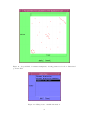
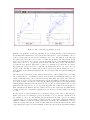
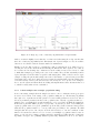
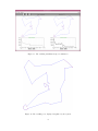
A first single run example: edge map recombination for the TSP . . . . . .
51
2.5.2
A first multiple runs example: population sizing . . . . . . . . . . . . . . .
56
2.5.3
Something less standard: crowding, preselection, deterministic crowding and
sharing schemes . . . . . . . . . . . . . . . . . . . . . . . . . . . . . . . . . .
63
A final and composite example: evolution strategies and elitist recombination/replacing . . . . . . . . . . . . . . . . . . . . . . . . . . . . . . . . . . .
76
Possible future extensions . . . . . . . . . . . . . . . . . . . . . . . . . . . . . . . .
79
2.5.4
2.6
iii
3 Recent optimization algorithms using a new approach to linkage learning
3.1
3.2
3.3
83
Linkage learning . . . . . . . . . . . . . . . . . . . . . . . . . . . . . . . . . . . . .
83
3.1.1
Laying the foundations and learning lessons: Genetic Algorithm
. . . . . .
84
3.1.2
Acknowledging the importance of linkage: Messy Genetic Algorithm . . . .
87
3.1.3
Taking shortcuts: Fast Messy Genetic Algorithm . . . . . . . . . . . . . . .
92
3.1.4
Neatly decomposing the search: Gene Expression Messy Genetic Algorithm
97
3.1.5
Not to put too fine a point on it: Linkage Learning Genetic Algorithm . . . 101
3.1.6
A different perspective: using a probability density estimator . . . . . . . . 104
3.1.7
Beyond linkage learning: scrutinizing the ways of natural evolution . . . . . 104
Linkage through explicit probability density estimators . . . . . . . . . . . . . . . . 105
3.2.1
In theory: MIMIC and beyond . . . . . . . . . . . . . . . . . . . . . . . . . 106
3.2.2
In practice: Implementing and using it in the EA Visualizer . . . . . . . . . 112
3.2.3
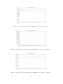
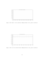
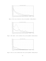
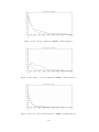
Running tests and analysing the results . . . . . . . . . . . . . . . . . . . . 114
3.2.4
Boundaries and differences . . . . . . . . . . . . . . . . . . . . . . . . . . . 142
3.2.5
Possible future extensions . . . . . . . . . . . . . . . . . . . . . . . . . . . . 154
Research conclusions . . . . . . . . . . . . . . . . . . . . . . . . . . . . . . . . . . . 155
4 Conclusions
157
A The EA Visualizer as an automated system
160
A.1 Creator classes . . . . . . . . . . . . . . . . . . . . . . . . . . . . . . . . . . . . . . 160
A.2 Name system . . . . . . . . . . . . . . . . . . . . . . . . . . . . . . . . . . . . . . . 170
A.3 The EA Visualizer editor . . . . . . . . . . . . . . . . . . . . . . . . . . . . . . . . 171
B Complexity of multiple runs EAs
175
B.1 Entering the settings . . . . . . . . . . . . . . . . . . . . . . . . . . . . . . . . . . . 176
B.2 Specifying the links . . . . . . . . . . . . . . . . . . . . . . . . . . . . . . . . . . . . 182
B.3 Enumerating the EAs and their settings . . . . . . . . . . . . . . . . . . . . . . . . 183
C EA Visualizer specifications, dimensions and history
iv
197
1
A general overview
In this introductory section we provide an overview of the contents of the remainder of the paper.
The preface at the beginning of the paper provided an introduction and pointed out what the
subject is that is adressed in this work. The actual elaboration is done in the sections that follow
the current one. As this elaboration is thorough and as a result rather large, it might be too much
to ask of an interested reader to continue and read the full contents of those sections. Giving
a good overview of what is presented or researched in those sections leaves it to the reader to
determine whether the full contents of the following sections is to be read and yet leaves him or
her with a good idea of what has been done in the light of this paper and what is discussed and
worked out further on. As such, this section extends the preface by starting from the subject of
interest introduced there and refrains from any type of detail that is used in the actual elaboration
that is done in subsequent sections, giving the reader a complete impression of the work in this
paper, without giving away the actual results.
The first and foremost point that this paper sets out to describe is the development of the EA
Visualizer. This includes the decisions on behalf of the contents of the system as well as implementation issues that concern establishing those contents. Setting up a large software system which
is what the EA Visualizer can become when set up right, requires a thorough investigation of the
requirements, followed by the design of a model and subsequently the actual implementation which
is in itself a cycle of validations and quality assesments that point back to more implementation
decisions and model descriptions. For each system, especially the lager ones, first a requirements
analysis needs to be conducted that tells us what is required from the resulting system, laying out
what we need to incorporate in the system model as well as the resulting implementation. It becomes clear that the requirements of the EA Visualizer are that the information can be visualized
both interactively and continuously, that the evolutionary algorithms in the system must be highly
expandable and component–wise reusable, that in order to be of any scientific value it requires to
have a multiple runs version that runs evolutionary algorithms a multiple of times independently
such that results can be combined to draw conclusions in the field of expected results, that the
system needs to be self–contained in that it has a help system that guides the user when needed,
that it must be easily expandable in more terms than just the algorithms themselves and that
Java applicability with respect to applets and thus usage directly over the web might be helpfull.
These requirements that follow from the analysis result in a number of constraints that the system
needs to constructed subject to, which is most important in the next phase of the engineering of
the software, being the construction of the model.
Before getting to that however, one point that resulted from the requirements analysis is of great
importance for what lies at the heart of the system, namely the EAs themselves. It becomes clear
that it is best to decompose EAs such that we get a component–wise description together with an
information flow through these components such that an EA is nothing more than a collection of
actual instances for each of the components in the decomposition. As such, the actual instances
for the different components need to be programmed only once and can then be used again
in every other EA. By doing this, we establish that the EAs in the system are very much so
expandable. As such, the first part in the modelling process is the decomposition of evolutionary
algorithms. Starting from a framework for EAs by Bäck [1], noting the shortcomings in both
detail and decomposition of EAs in this framework and subsequently expanding it to overcome
these problems, a decomposition is reached that holds great expressional power with respect to
evolutionary algorithms. The decomposition that thus results holds twelve components ranging
from obvious such as the Recombinator and the Genotype to perhaps more unexpected such as the
Similarity and the Mater. Based on this decomposition, the engine that lies at the heart of the EA
Visualizer is easily created in its most basic form by implementing the information flow through
the components and letting the components themselves do virtually all of the work. When the
actual instances that are to be used for the components in the decomposition are provided, such
an engine can be created by the system and started to actually run the EA. A mechanism using
1
information objects is then used to gather information about the algorithm and thereby we have
modelled (and almost implemented) the heart of the EA Visualizer.
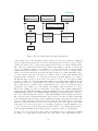
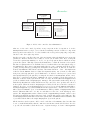
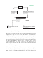
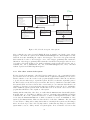
Looking toward the requirements of viewing the results from the EAs, an MVC type of model is
created for the system in which the model within the MVC is the engine just described, the viewer
is a new class that is a container for views which are fed with the information coming from the
model and the controller is the EAVisualizer class itself that is the main class and takes care of
data flow in the system, which is mainly from the engine to the views, but also directly from the
user to the system through mouse clicks and so on. Elaborating upon this MVC type of model
description of the system, a general name system is introduced that allows for unique naming in
the EA Visualizer and creator classes that are capable of creating instances for the components
in the decomposition and views to actually perform the visualization. By setting up these classes
as general and strictly according to rules as possible, the next step can be taken in creating a
fully–fledged system that automizes updating the system with respect to the data administration
required to notify the system of the presence of new instances or views. The actual result will
be an even more powerfull editor version of the system that is capable of expanding the system
in more ways than just mentioned, but such is found in the actual elaboration that is started in
section 2. The editor is a complex task and brings along a large model that also incorporates the
help system. Furthermore as many parts of the system are parameterized, a special structure for
parameter definitions is required that also allows for automatic expansion towards multiple runs
versions as such is to be facilitated by the system without extra requirements from the user.
Modelling the viewer brings along the definition of internal and external views that are mostly
used for direct graphical visualizations and numeric visualizations respectively although such is
not a constraint and thus it is possible to visualize information graphically in external views and
numerically in internal views. All views are updated as the EA runs. It must be possible to define
multiple runs and single runs views as different entities because running multiple runs or single
runs mostly results in visualizing information in a different way (averaging results over multiple
runs in graphs for instance or viewing the population contents for a single run). These different
type of views are then updated through a slightly different mechanism that distinguishes a normal
update from a termination update.
The implementation that follows brings along many details. Creating fully automated operations
such as offered through the editor version of the system and the facilitation of multiple runs is a
complex task and details to this end are placed in appendices A and B respectively. In this section
we wish to refrain from any implementation details and leave this for as much as is interesting
for the actual elaboration as found in section 2. That section closes with a demonstration of the
resulting system by guiding the reader through a number of examples of EAs, both in a single run
and over multiple runs.
The system that so results is ready to be used for testing evolutionary algorithms. Creating
the system to be ready for this is a very time–consuming task as we are referring to the actual
implementation which is greatly vast for the general framework constructed together with its
complex automated tasks. Also in order to demonstrate the system, a number of instances and
views need to be actually implemented in order to work with the system and visualize any results
at all. This requires even more time, not to mention writing the code comment in a proper fashion
during development as well as the help files in the system. To get an idea of the size and contents of
the resulting system, we refer the reader to appendix C. In any way, when all the implementations
are finally finished, we can indeed use the system to investigate the interesting new algorithms for
optimization that use a different approach to linkage learning. In order to do this, an overview of
what linkage learning is, where it came from and why it is required is given first. We refrain from
going over the descriptions of the algorithms described in the process of doing so and state only
that an historic overview is given which shows when the notion of tight linkage was introduced
and resulted in linkage learning approaches. In this historic overview, the classical GA is visited
as well as the mGA, the fmGA, the GEMGA and the LLGA. After thus having made clear what
linkage learning is about, the recent algorithms with a different approach to linkage learning are
2
introduced. Using the historic overview of the GAs that were evolved along the lines of the classic
GA, the new approaches can be put in perspective by the reader.
After the introduction and the description of what linkage itself means, tests are run to investigate
the competence of the recent new approaches. At first a couple of tests are run and compared to the
classic GA. Based on results so achieved, it becomes clear that a number of items are interesting
for further directed research. It is chosen to investigate the difference between the two recent
algorithms that are introduced and to hopefully along those lines also find information about the
boundaries of the approaches. As the main point however, we set out to find the implications of
the difference between the two approaches that are MIMIC [6] and an approach by Baluja and
Davies [3] that is supposedly an improvement over MIMIC. The results thus obtained are the final
research results within this paper and the reader can read them directly if desired in section 3.3 as
we shall refrain from duplicating those results here. Also as the time span in which the research
was to be conveyed was unfortunately not too great as a good and usefull implementation of the
EA Visualizer took a great deal of time. A number of topics are pointed out as a result from the
testing that are interesting to visit as future research.
The testing in both the undirected and directed way results in a good insights as to how the recent
new algorithms work. When relations are clearly required to be respected, the new approaches
show an improvement over the classical GA, however it is unclear yet to what extent the complexity
of the relations can be so that the new approaches are still capable of finding the right linkage to
solve the problem at all.
This paper closes by drawing conclusions on the full contents of the work that was done and is
described in the text that follows up on this overview section. As noted above, details of the system
are incorporated in appendices to give the reader an idea of the complexity of the implementation
and the convenience offered to the user by the automation that is thereby thus introduced. We
close this overview section by noting that the testing of the recent new approaches in the EA
Visualizer system is itself a test of the expressional power introduced by the decomposition as the
new approaches aren’t exactly standard GA material. However, they are evolutionary approaches
and the decomposition proves to indeed be a powerfull description of EAs in general as the new
approaches fit into the EA Visualizer without a problem, which is also the case for the different
GAs that were described along the historic line that is provided on behalf of the explanation of
linkage learning as even though they are not implemented, they are shown and explained how to
fit in the system through implementation of new instances for components in the decomposition
solely.
The remainder of this paper is organized as follows. A specification of the EA Visualizer system
is given in section 2. This specification includes both the model design as well as some implementation issues. In section 3 the notion of linkage learning is introduced as well as the two recent
optimization algorithms that use a different approach to linkage learning. Furthermore, the results
of the tests as mentioned above are presented and investigated so as to finally be able to draw
conclusions with respect to the competence of the new algorithms. In section 4 the final conclusions are drawn with respect to the material described in sections 3 and 2. In three appendices,
detailed information is incorporated with respect to the EA Visualizer system. In appendix A it
is explained how the system was made capable of being a fully automated system that includes an
editor. Appendix B contains a description of the complex implementation of multiple runs EAs.
Finally, in appendix C background information is given on the resulting system that is the EA
Visualizer.
3
2
The EA Visualizer
The creation of large software systems of whatever kind is a process that is always divided over
at least a few steps or layers. At the least it is very important to have a good model of the
system in order to build something solid. This section describes the complete engineering of the
EA Visualizer system. This ranges from analysing what the system should be capable of to the
specification of the integration of evolutionary algorithms to implementation details.
In section 2.1 a survey is done of what functionality it is exactly that we want the system to have.
It is decided what it is we want to use the system for and how broad our perspective should be
with respect to evolutionary algorithms. This latter aspect is made precise in section 2.2, where
according to the determined measure of granularity, the general framework of any evolutionary
algorithm within the system is specified. In order to establish this, the highly idealized description
of the evolution process that are evolutionary algorithms is divided over a certain amount of
evolutionary components. The modelling of the system in an object oriented fashion is done in
section 2.3. Some of the implementation details are discussed in section 2.4 and examples regarding
the usage of the system are given in section 2.5. Finally, in section 2.6 the resulting system is
evaluated in retrospective, glancing at options for future further enhancement.
2.1
Requirements analysis
In this section we describe what is required in order to establish a system as generally described in
the preface. We have seen that the system should have two important properties, namely that of
the interactive and continuous visualization of data and the expandability of the system through
modularity of the evolution process. It is these issues that we will examine closer.
2.1.1
Visualizing information
Starting with the visualization side, in order to establish a flexible and expandable system with
respect to the visualization/viewing part as well, this part of the system should be separated from
the evolution process as much as possible. Furthermore it should have a highly modular structure
so as to make it possible for the user to only define what it is that should be shown and how. The
user should not be bothered with applying changes to the system in order to utilize the new view.
This perspective leads to a MVC (Model–View–Controller) type of system in which the model
(the evolution process) is separated from the view (the visualization part) and the system itself is
controlled by the controller (the EA Visualizer ).
Establishing the continuity of the visualization means that the controller will have to transfer
information from the model to the controller after each generational step. Once the process has
reached the next generation, all views should be updated by the system with the new data. It is
then left to the views to decide if they need to provide the user with new information.
The other required aspect of the viewing system is for it to be interactive. We should be carefull
when stating what level of interaction we allow the user to have with the system. If we want to
have a direct influence on the evolution process through the views, the MVC separation as stated
before becomes harder to establish as working with the views can then hold that the model should
change directly. Furthermore if we are to create a modular setting for the evolutionary algorithms,
allowing a change in settings directly through interaction with the views at a metalevel has no
obvious or user–friendly definition. Next to that more problems arise when some combinations
of components are not allowed (fitness functions are defined for certain genotypes for instance).
This issue is not too difficult to resolve though because the viewing system should get all the
information from the model as we cannot know in advance what it is a new view is going to
visualize. This means that all instances of the components of the current evolution process will
4
be passed on to the viewing system along with all information on what the instances have done
the passed generation. As such any interactivity that is desired to alter parameters directly can
be implemented as desired in a new view, as long as the views are allowed to receive input. It
is therefore only required to make the system pass input information from the user to the views.
This should at least be established for a mouse pointing device. By doing this, we will create a
possibility of a far reaching form of interaction that extends from altering view characteristics to
having an influence on the current evolution process.
2.1.2
Expandability for EA’s
It is stated in the introduction in the preface that the system should allow for expandibility so
as to easily compose evolutionary algorithms. A modular decomposition of the evolution process
results in a description that consists of some components. The evolutionary algorithm uses these
components and passes the required data between them. By doing this, a high level of expandability is created as each component of this definition can have a multiple of instances. The user never
has to redefine the entire process. When for instance a new recombination operator is thought of
for genetic algorithms, this recombination operator can be implemented without having to implement the binary string genomes, the desired fitness function and so on. Merely the recombination
operator has to be defined. When using the system, the desired instances are selected to be part
of the evolutionary algorithm without any changes whatsoever to the structure of the system.
This approach also has a drawback. By specifying any general framework except that of total
freedom, the evolutionary algorithms that can be created are of a certain form. This implies
that in order to have a general applicable system, the expressional power must be great. This is
something of a problem though because evolutionary algorithms are subject to ideas and visions of
many people and are therefore increasingly not conform to a specified structure. Nevertheless, in
order to create a system that is easily utilized, it should be noted that the majority of evolutionary
algorithms can be described within a general framework and this framework need not even be all
too complex. Very specific evolutionary algorithms that go beyond the usage of single populations
are harder to place within such a framework, but by not making certain requirements too explicit,
even these types of evolutionary algorithms can be fit into one general framework.
By using such a structure, the evolutionary algorithm can be “clicked” together with ease. Furthermore, writing code for instances of components creates evolutionary utilities that can be used
within other evolutionary algorithms without having to incorporate them over and over again. As
the exact decomposition of the evolution process conform to which the evolutionary algorithms
within the EA Visualizer will be composed is a fundamental issue determining the final applicability of the system in this field, a seperate section is devoted to this issue (section 2.2).
2.1.3
Single run and multiple runs
Evolutionary algorithms belong to the class of probabilistic algorithms because of their random
aspect in applying operators with a specified chance, the creation of random genomes, etc. As
such we can never rely on these algorithms in one single run to provide us with information from
which we can then draw conclusions on how good or bad it is in any sense. It is for this reason that
all experiments with evolutionary algorithms are always (or at least should always be) performed
a multiple of times. The results over these runs are then combined (for instance by averaging).
The whole idea of setting up the EA Visualizer has been to create a new way to look at evolutionary algorithms, namely through interactive visualizations. As multiple runs are mostly conveyed
when the user is occupying him or herself with other activities because they take a lot of time,
these interactive visualizations imply the main utilization of the EA Visualizer be through the
usage of single runs.
5
Nevertheless, the position of these single runs and the interactive visualizations within the research
should be reviewed here. Not only are indeed continuous and interactive visualizations a great
tool to learn about and research evolutionary algorithms, they are also a way to quickly establish
satisfaction regarding intuitions. In order to then generate a thorough investigation, a multiple of
runs is still needed. Next to that, using the single run version on beforehand guards the user from
wasting a lot of time in computing results over a multiple of runs on wrong settings. Still in the
end, the user will want to be able to perform a multiple of runs with different settings in order
to compare results. It is important to realize that a general system for evolutionary algorithms is
not complete or even nearly worthless if in the end one is not capable of running an algorithm a
multiple of times and combining the results.
Furthermore, not only is it common practise (not only for evolutionary algorithms) to test an
algorithm a multiple of times, but also to test it on problems with a different size or with different
settings for the algorithm. As such, the availability of a multiple runs version that provides the
option for running algorithms with different settings of all kinds is always a valuable and almost
indispensable property.
2.1.4
Self contained systems
As is the case with an increasing amount of common systems these days, software distributions
are intendend to be self contained. This implies that the software is all that is needed to get
the system working and more importantly, to work with the system. Such is ofcourse a desirable
property because it releaves the author from the writing of large documents like user manuals.
As the whole structure of the EA Visualizer will be a modular one, conform to the issues discussed
above, a help system that contains information for every component in the system will allow
for the system to become self contained on the condition that extensions to the system in new
instances of the components can be and are documented properly within this help system. From
the implementation view this implies that the help system is user friendly, allowing the user to
click links to navigate between documents and so forth. Furthermore, the help system must be
easily extendable so as to not make it an unattractive job to write help documentation for newly
added instances. Finally, the help system must ofcourse be easily accessible from every part of
the system.
Setting up a help system as described allows the system to be expanded world wide in a uniform way, allowing users to swap implementations without problems together with documentation
within one system. This implies that all can be done electronically and without any overhead
which makes the system yet even more attractive.
2.1.5
Easily expandable systems
An important property of quality systems is expandability. It is desirable to have a good modelling
and a good implementation of some problem or algorithm within a larger system such that it offers
user friendly operations and levels of abstraction, but in the long run, expandability plays the most
important role.
So far we have seen that the EA Visualizer will be set up in a modular way with respect to many
parts of the system. This is a very strong fundamentation on which to base the achievement of
expandability. If we are capable of decomposing the system in such a way that parts are designed
by descriptions such that implementations can be made in whatever way desired as long as they
meet the demands of the description, we have a potentially expandable system. This is exactly
the case with the EA Visualizer as argued in sections 2.1.1 and 2.1.2.
By achieving this, the system is not yet easily expandable, because certain parts may be significant
within the system, as is the case with the EA Visualizer. This can imply that the system needs
6
information on beforehand in order to work with the instances. This information could for example
be a name that is administered in a name system to maintain consistency. The point is that
adding new instances to the system will be accompanied by some means of an announcement
to the system. This announcement becomes more difficult as separate systems or factories are
created that maintain system information with respect to these instances and their availability to
the system.
In order to once again make sure that extending the system does not become too unattractive
so that the expandability property is lost after all, the system administration should be made as
mechanical as possible so that extensions can easily and unambiguously be achieved. When we
push this into a mechanical form, we can even form this extension process into a protocol form
of action so that we can automate this as a system update operation. Such is a very desirable
property.
Creating the editor makes using and expanding the EA Visualizer system even more attractive
because just like taking away the overhead of the design and implementation of the complete
evolutionary algorithm, the data flow within it and the data flow to the view part of the system,
an editor takes away the overhead of updating and perhaps recompiling the system by hand, which
in turn increases the self containedness of the system.
2.1.6
JAVA applicability
As we are to develop the system in the object oriented language Java we should ask ourselves
the question what level of applicability we desire to have for the resulting program. Like most
programming languages, Java can be used for the creation of programs that work on a computer
under a certain operating system. In this respect it is no different from C or Pascal. One well
known important difference is ofcourse the fact that Java is platform independent so we do not
need to worry about which platform to choose to create the application for. Next to this great
property, Java also comes in two approaches. Next to the normal programming language, Java
also offers the option to create Applet classes that can be used in a WWW browser. As such,
the resulting program is easily brought amongst a wide public around the world. There is an
important sacrifice we must make though when choosing to develop the program so that it also
works as an Applet. The point is that Applets are not allowed to write to files as opposed to
a normal application. This means that any results from algorithms that are normally written to
disk or any settings that would be saved in some way can only be permanently stored if this is
done by some other program that is running on the computer after using some copy and paste
routine of the operating system. This latter type of operation is increasingly easy these days so
this doesn’t withold us from creating the option to not only distribute it over the web but also to
put it on–line so that users can directly use the program when surfing the Internet.
Before closing this section, we note that any editor version of the program cannot be supplied
as an Applet because we must be able to save in that program as that is the larger part of the
functionality of it. So in conclusion we can say that the final application will created without any
option to save data in whatever way with the exception of the editor version of the program.
2.1.7
Summary
In the above we have analysed what is required in order to build the system that was in a coarse
grained way stated in section 1. In order to actually design a system model and implement the
system based upon that model, we summarize the requirements.
1. The system should have a modular structure, decomposing the intended to be most flexible
parts to an extent that they are easily expanded. This means that
7
(a) visualizing the system is done by views that are implemented as seperate classes just
as
(b) the instances for the components of the evolutionary algorithm are implemented separately so that in working with the system a specific evolutionary algorithm is created
by selecting what implementations to use for the components.
2. The views should be capable of processing user input at the least by using a mouse pointing
device, making the visualization interactive.
3. The EA Visualizer as a controller should transfer information from the model to the views,
transferring everything that could be of interest and as such allowing every view to be
completely general or entirely specific as well as to offer an interaction that can indeed have
a direct influence on the evolutionary algorithm.
4. The evolutionary algorithms that can be constructed within the system should be described
by a general framework that is a decomposition of the evolutionary process. This decomposition should be made such that it holds a great amount of expressional power, but needs
not to be defined for all specific cases, making it inherently too complex.
5. The EA Visualizer should offer the possibility of running evolutionary algorithms a single
run as well as a multiple amount of runs in which in the latter a multiple of combinations of
parameters can be set as well as a multiple of runs for each combination of parameters (and
component instances).
6. The system should be self–contained through the containment of an easy to use extensive
help system. This help system must be expandable for every other part of the EA Visualizer
that is expandable.
7. The implementation of the EA Visualizer should be such that administration of all parts
that can be extended is done in a mechanical way so that it can be automated, leading to
the editor version of the system allowing for easy editing and expanding of the system.
8. The implementation should refrain from saving information to disk with the exception of
the editor version of the program. This should result in the possibility to create an Applet
version of the program that can be put on–line on the WWW.
2.2
Decomposition of evolutionary algorithms
In section 2.1 we have argued that the evolutionary algorithm should be decomposed. This means
that we are to create a general framework in which we identify the components that have a clear
and distinct functionality. As we shall implement the system in an object oriented language, a
class will be created for each such object. We have argued furthermore that these classes should
be a definition of what the components should be capable of. Instances of these classes will then
be components that can actually be used for the task defined. To be more exact and more with
respect to a Java implementation, these components will become abstract classes that cannot be
instantiated. The instances that can actually be used will be the instances of subclasses of these
components that specify how the functionality is exactly established.
2.2.1
Coarse grained decomposition
In order to create the decomposition, we distuingish two levels of precision. At the top level we
are not concerned with how the evolution exactly takes place. We can see this as a coarse grained
decomposition. At this level we define the most general framework which has become common in
all approaches within evolutionary computation and as such is found in every type of evolutionary
8
Initialize
(Generate population, evaluate genomes)
Terminator:
Should the EA
terminate now?
Yes
No
Terminate
Evolve
(Determine and/or create the genomes
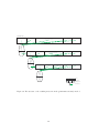
of the next generation and evaluate them)
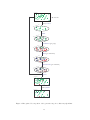
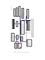
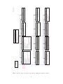
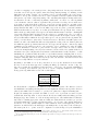
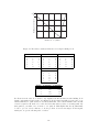
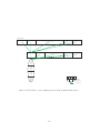
Figure 1: Coarse grained decomposition of evolutionary algorithms.
algorithm. This intersection of evolutionary algorithms is displayed in figure 1. Firstly, as is the
case in almost every algorithm in every discipline, we have an initialisation phase. We generate
the first generation genomes (most often at random) and evaluate their fitness values. Once this
is done, we can perfom the body of the algorithm. As can be seen in the figure, this amounts to
checking first whether the algorithm should be terminated on any behalf whatsoever (frequently
used conditions are the amount of the genomes and the diversity of the population members). If
this is the case, the algorithm halts and enters the terminated state. Otherwise, an evolution step
is performed, bringing the population to the next generation. At this precision level we make no
attempt as to specify further how this is established. All we require is that any new genomes in
the population be evaluated so as to establish the invariant that every member of the population
has been evaluated (so its fitness value is known) when the termination condition is to be checked.
After this evolution step, the algorithm has reached the next generation and the termination
condition is checked again.
From this top level model for evolutionary algorithms we can already derive a few components
that are part of the decomposition. In the figure, this has been insinuated by suggestively posing
the question “Should the EA terminate now?” to something named a Terminator. It is clear
that we can vary the termination condition that is to be used. A termination condition can be
based upon any information from the evolutionary algorithm. Modelling such a condition leads
to a separate component which is named Terminator. This component signals based upon all
information from the last generation step and the current state of the algorithm whether or not
the algorithm should terminate.
Continuing in this manner, we could argue that the initialization process can be modelled within a
component named Initializor. This component would then be requested to generate new offspring
at the beginning of the algorithm. However, if we take a step back and view upon the framework
from a global perspective instead of a component–wise one, we have already missed two of the most
important components that are implicitly present in every evolutionary algorithm. These are the
Genotype and the Population components. A subclass of the Genotype component is a description
of what genetic material is used. It is a description of the material that is available to code solutions
with. The Genotype component will therefore define access to fitness values and so forth for actual
genomes that will occur in the population during the run of an algorithm. It cannot define relations
with respect to the genetic material as this differs for each actual Genotype (like binary strings
9
or evolution strategies tuples). The Genotype component is closely related to the Population
component because the population consists of genomes. The Population component is therefore
some collection that will for instance allow for adding and removing genomes. This component
is also the component that holds information with respect to the global perspective in that it
possibly defines relations between the individual genomes (such as clusters or subpopulations).
It is important to see that these components are of the greatest of fundamental importance as
they allow for data storage. These components are never so obviously present in schematics or
algorithm descriptions because these mainly consist of the usage of operators, which are obviously
transformed to components according to our decomposition approach. We have identified the
Genotype and the Population as fundamental components however and are therefore indispensable.
We should also note that the fundamentality of these components could play an important role in
the implementation of the general framework conform this decomposition. If we now look again
at the part from figure 1 that lead to the definition of the two fundamental components Genotype
and Population, the “Initialize” step, we can argue that a separate Initializor is superfluous. We
can easily assign this functionality to the just discovered fundamental components. This implies
that we define the Population component to be such that it can renew the entire population.
This argument however is normally not strong enough to keep us from implementing that new
component as it provides us with a higher degree of freedom. However, it also increases the
complexity of the system as all these components are linked. Such is the case ofcourse for each
of the components. The most important point is that initialization is in almost every case done
at random, causing the addition of a new component to make the process more complex than
need be. In the few cases that random initialization is not favored, we should note that we have
not done away with the possibility of altering this phase of the evolutionary algorithm. We have
only reduced the number of degress of freedom in putting an evolutionary algorithm together by
selecting instances for its components. This reduction in amount of degrees of freedom has been
justified by the argument that the dispensed degree of freedom is hardly ever utilized.
Finally, the least obvious part of figure 1 is the explanatory text between brackets. In these texts,
it is twice mentioned that the genomes in the population need to be evaluated. Evaluation is always
done by using a fitness function. Just as much as the Genotype and Population components, the
Fitness Function is a fundamental component of every evolutionary algorithm. It is this part that
can provide us with the information whether one genome is in some sense better than another.
Moreover, the fitness function holds information regarding the domain. For instance, it contains
information regarding distances between cities for a TSP instance. As such, this component has
an important task beyond providing fitness values. It is also a holder of environment or domain
information.
2.2.2
Fine grained decomposition
The part from figure 1 that has not been discussed yet, is the Evolve step. We cannot derive
a new component from this, because it is a composite step. It is this step that we have argued
in section 2.1 to decompose resulting in a high expressional power for composing evolutionary
algorithms. In the light of the setting in this section, this is the second level of precision. We are
now to make exact how to transform the state of the evolutionary algorithm from one generation
to the next. This requires a fine grained decomposition.
In oder to obtain such a fine grained decomposition, we could regard general algorithm descriptions
that have already been made, such as the following that was posed by Bäck [1]:
t=0
initialize(P (t))
evaluate(P (t))
while not terminate(P (t)) do
t=t+1
10
P (t) = select(P (t − 1))
recombine(P (t))
mutate(P (t))
evaluate(P (t))
od
In this scheme, P (t) denotes the population in generation t. This framework certainly contains
essential operators such as selection and recombination. Furthermore, we recognise components
that we have already identified in the coarse grained decomposition. We shall look at each of the
operators from the above general framework by Bäck more closely (not in the same order) and
determine what components to define on behalf of them.
Recombine
Recombination is the most prominent operator in evolutionary algorithms. The combination of
genetic material that establishes the genetic exploration of the search space is classical and accepted
to be the most important together with selection. This operator needs no further introduction and
it is no less than required that it be a separate component in the decomposition. Just as we had
the Terminator for the termination condition, we now have a Recombinator for the recombination
operator.
It is important to determine what the input and output of the Recombinator component are. The
algorithm by Bäck refrains from any specific details as it merely states that recombination be
applied to the members of the population. More specific however, if we for instance look at the
classical one–point crossover operator from genetic algorithms, it takes two parent genomes and
generates either one or two offspring genomes. This is a better description of the recombination
operator and it is only a logical definition to state that the Recombinator component takes as
input a collection of parent genomes and returns a collection of offspring genomes. It is then up
the general framework to supply the Recombinator with the parent collections that it wants to
have recombined. It is this definition that we shall use.
While we are looking more precisely at the definition of the Recombinator component and having
achieved the definition by looking at the one–point crossover operator from genetic algorithms, we
could look a bit closer at this specific recombination operator. A fundamental issue in the definition
of this operator, is the selection of a crossoverpoint. This selection is done at random. This is a
good point to remember that evolutionary algorithms belong to the class of probabilistic algorithms
and as such make use of pseudo random number generators. In the case of evolutionary algorithms,
pseudo random number generators are even used many times during one run. It is therefore
important to note that a good pseudo random number generator is of the utmost importance.
Because of this, we should have a seperate Pseudo Random Number Generator component which
is just as the Genotype, Population and Fitness Function components a fundamental component.
Mutate
An other operator that is frequently used in evolutionary algorithms and was regarded an essential
operator in the early stages of evolutionary computation, is mutation. It is an operator that is
included within evolutionary algorithms to follow the Darwinistic approach of random mutations.
Just as the Recombinator component, this operator needs no further introduction as it is a classical
one. It follows that we will require a Mutator component in the decomposition. We have already
seen that random numbers are needed when we discussed the recombination operator. It is now
even more obvious that these are needed, as mutation is almost always implemented as an operator
that alters a genome in a random fashion.
Just as with recombination, the framework stated by Bäck refrains from filling in the details with
respect to the application of mutation to the genomes in the population. When we regard the
mutation operator by itself however, we should note that it is an operator that alters exactly one
genome. We therefore define the Mutator component to have as input one genome and to output
another genome which is a mutated version of the input. The general framework will then have
11
to specify how to mutate all genomes.
Select
Together with recombination, the selection operator is known to be the most essential to the
evolution process. Selecting in some way the better of the genomes in the population, this operator
provides the search with a drift. There are many ways to select genomes from a population, but
like can be seen from Bäck’s algorithm, selection takes place before recombination and mutation.
A more precise definition of the selection operator is that this operator selects the genomes that
will serve as parents to generate offspring. There is one problem with this definition, namely that
when we use the selection operator to, as it is stated in this definition, select genomes to serve as
parents and then use them to generate offspring through recombination and subsequent mutation,
there is no way of telling what genomes will be present in the next generation. Strictly speaking,
in the former sentence we have no new genomes in the population whatsoever, since we have only
made a selection from the old population and placed the results in a void. How then is this done
in the general framework by Bäck?
If we look closely, we see that the selection operator is used in such a way that the selected
parents replace the entire current population. From the looks of the remainder of the algorithm,
recombination and mutation then directly alter these genomes within the population, whereas
we have so far defined these two operators to create new genomes. Furthermore, the replacing
of the entire population with the selected genomes might very well not be a satisfactory way
to incorporate the genomes of the next generation. We could desire to in some way merge the
genomes in the current population with the offspring genomes. This leads to the definition of a new
component. It is a too strong requirement to state that based upon the selection on beforehand
we are to continue the rest of the evolution process, forgetting the contents of the population
at the current time. This would neither do justice to the definition of the traditional selection
operator as just stated above. So in order to offer the possibility of merging the genomes of the
current population with the offspring into the population of the next generation, we define to
have a Replacer component that implements a replacement strategy. The input to a Replacer is
the final collection of offspring genomes (after recombination, mutation, etc.) together with the
current population. The output is a void as the component is to replace the genomes of the current
population in some way, implying that the population is altered. So the Replacer component has
a side effect in that it alters the current population.
We should now ask ourselves if we are content with the degree to which we are capable to select
genomes either before or after creating offspring. The complete selection process now consists of
the selection of parent genomes before generating offspring and placing the offspring within the
current population after creating offspring. This is to a large extend satisfactory and contains
a great expressional power with respect to the selection mechanism. For instance, the standard
selection mechanism that allows us to clear the entire contents of the current population and replace
it with only the offspring genomes is now achieved by using a selection mechanism to select the
parents in any way that might be preferred (such as tournament or roulettewheel selection) and
using a replacement strategy that only keeps the offspring genomes. Special selection strategies
like for instance the (µ, λ) and (µ + λ) (µ parents, λ offspring) selection strategies from evolution
strategies can now be incorporated as well. For instance when we desire to have a (µ, λ) selection
mechanism (select surviving genomes from the λ offspring), we can implement the replacement
strategy to be such that like with the standard selection mechanism it only keeps the offspring
genomes, but it also applies some form of selection to those offspring. For (µ + λ), the replacement
strategy would do almost the same, but the selection would then be from the total of offspring
and parents.
Next to now being able to merge the genomes from the current population with the offspring,
the Replacer component also allows us to establish an invariant with respect to the population
size, which is a desirable property. We now need not to generate offspring and wait for the next
round to be able to apply selection again (perhaps even in two phases so as to first select the
surviving genomes and then the genomes that are to serve as parents). We can now use the
12
Replacer component to maintain the correct amount of genomes in the population. This means
we have a nice invariant and that we can terminate the algorithm after each generational step (the
Evolve step from figure 1.
Still there is one thing that is not satisfactory. This follows from the discussion above about
implementing (µ, λ) and (µ+λ) selection strategies. We have argued there that implementing these
strategies requires a selection functionality incorporated in the Replacer component. This implies
that the framework will have the undesirable property of a need for code duplication. It follows
from the discussion that we need to select genomes within the Replacer component. If we would
want this selection to be a tournament selection, we would have to redefine it within the Replacer
component as we ofcourse already have defined it for the selection operator. Such is very much
undesirable. If we look closer, we see that we have implictly defined a composite functionality for
the Replacer component. We had done this earlier with the Genotype and Population components
with respect to the initialisation phase in section 2.2.1. In that case, the composition was argued to
have no undesirable results at all. In this case however we need to factorize the current definition
of the Replacer. Better put, we need to specify the definition of the Replacer more exact and
introduce a new component.
If we are to remove the necessity for a selection part in some cases within the Replacer, we need
to put a another selection operator directly after it. Then there is no need for a replacement
strategy to have to select any genomes to survive, because this is done by the second selection
operator. The Replacer than remains the same as before with exactly the same input and output,
but without a possible selection property.
We have now come to the point where we can sum up the components that we shall use in the
general framework. According to Bäck’s framework we have a Selector component that selects from
the population a certain amount of genomes. Furthermore we have a Replacer component that
replaces the contents of the current population with a collection of offspring genomes according to
some strategy. The application of the Selector component is twofold, whereas the application of
the Replacer component is required once. The Selector component is used once at the beginning
of a generation step to select the genomes that will serve as parents. The Selector component is
then used again at the end of a generation step, directly after the Replacer component to select the
genomes that are to finally survive the current generation step. As these two selection strategies
need not be the same, we should facilitate in the definition of Selector components only once, but
utilize them in two different locations. As such, we have two new components, namely the Selector
and the Replacer, in which the Selector is defined once and used as a component twice, leading
actually to three new components.
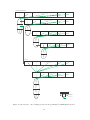
Putting the components together
We have now completely gone over the algorithm by Bäck that was stated at the beginning of this
subsection. We shall therefore now review what we have discussed so far. To do this in the most
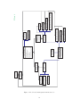
brief way, we extend the general framework:
t=0
initialize(P (t))
evaluate(P (t))
while not terminate(P (t)) do
sel = select(P (t))
rec = recombine(sel)
mut = mutate(rec)
rep = replace( mut, P (t) )
P (t + 1) = select(rep)
evaluate(P (t + 1 ))
t=t+1
od
13
We have been more precise in the framework by stating what happens with the genomes that were
selected, recombined and so on. We should note however that not everything is clear yet. For
instance, after the before selection, recombination is applied to the result of the Before Selector.
We have argued that the functionality of the Recombinator is defined with respect to a collection
of parent genomes. The result from the selection however is a merely a set of genomes that are
to serve as parents. It is most certainly not (always) the case that these genomes are all to be
parents, generating offspring together. In genetic algorithms with one–point crossover, two parent
genomes are required to apply the recombination operator. From a population of 100 members for
instance, we might select 100 genomes (selecting some genomes most likely twice or more often)
and make subsets of size two from this large set of genomes. These subsets can then be recombined
one by one. Indeed, to go from the selection of genomes for offspring generation to the sets of
parents that are actually recombined, we need some sort of mechanism.
Putting genomes togther is called a mating mechanism. It is therefore that we shall incorporate
a new component in the general framework, called the Mater. This component has as input a
collection of genomes and returns a set of sets of mated genomes, or in other words parents that
have been put together to undergo recombination.
Continuing the inspection of the extended algorithm, we find that the specification of the application of mutation is not exact enough. We have already defined however that mutation is an
operator that is to be applied to individual genomes. What we need to specify therefore within
the algorithm is that we mutate every genome independently. Other than that, the algorithm has
no unclear parts that lack detail.
An important property that has shown to improve the speed of evolutionary algorithms as well
as their results is the consideration of problem specific knowledge in terms of non–evolutionary
operators. These external approximation techniques that are mostly heuristics are applied to
evolutionary algorithms so as to speed up the search for meaningfull genomes. This is especially
desirable when the search space is rather large (for instance with N P complete problems). An
example is the incorporation of a two–opt heuristic for TSP instances or a first–fit heuristic for
bin–packing. Incorporating heuristics like these, makes an evolutionary algorithm be called hybrid.
Just as the mutation operator, this “operator” is applied to every genome individually. Therefore it
poses nothing new with respect to the framework, only an extension of what we have already seen.
Concluding, we will allow for hybrid evolutionary algorithms by incorporating a new component
called Hybrid Searcher.
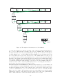
We could now say that we have a full decomposition with a general framework that does not
remain vague with respect to details and that holds a great expressiveness to define evolutionary
algorithms. There is only one thing that is important and not yet present in the decomposition.
One tends to easily forget about this component as it is rather invisible, even more than the
Genotype and the Fitness Function components. It is common practise to compare genomes in
some way, be it in a genotypic or phenotypic fashion. Moreover, when working on multimodal
optimization, a measure of similarity is a very important item. Note that the framework is already
complete in the sense that this type of information can be incorporated inside the components that
are already present. However, if we were to not separate this similarity functionality and make it
into a seperate component, we will once again have the situation we had before when we came to
the conclusion that a second selection operator is needed. Therefore, we define that a Similarity
component is part of the decomposition. It is nowhere visible in a framework description or figure,
but it is passed on to the components so they can use this component, just like the pseudo random
number generator. This component can be seen as fundamental as well, because it is used by other
components. Its fundamentality is less obvious, but under a different naming this will become clear
in the next section.
This concludes the decomposition of evolutionary algorithms. After inspecting evolutionary algorithms at two levels of granularity, we are now ready to state the resulting general framework
and its components, both visible and invisible within the general algorithm that is part of the
14
framework.
2.2.3
The final general framework conform the decomposition
In sections 2.2.1 and 2.2.2 we have deduced in a constructive way the components that need to
be part of a general framework for evolutionary algorithms. This decomposition has led to the
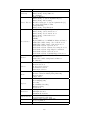
definition of the following components:
Name
Population
Fitness Function
Genotype
Hybrid Searcher
Mater
Description
A Population is a container for the genomes. When looked upon as a storage facility, the Population is nothing more than a collection of objects,
but in the evolutionary algorithm it can come to hold more information
than just such. For instance information on clusters or linkage between
genomes can also be incorporated here, making the Population vastly more
important than merely the holder of a collection of genomes. Like the Fitness Function, the Population serves as an environment. The difference is
that the environment induced by the Population regards information about
the structure and the linkage between genomes as opposed to information
regarding the search space of the optimization problem.
The Fitness Function rates the genomes and therefore the solutions according to their fitness. Very important alongside this definition is the fact that
the Fitness Function ofcourse also defines what a “better” fitness value is
(maximization or minimization for instance). Observing this definition in
terms of the algorithm, it is clear that the Fitness Function defines a mapping from the solution space to the real numbers. This points out that
the Fitness Function plays the role of the environment in the optimization
problem. It holds the information that is specific for the problem instance.
Finally, the Fitness Function implicitly defines a genotype-phenotype mapping. To be more precise, it denotes the exact location in the problem space
for each genome. It is clear that based on this location, the Fitness Function
computes its fitness values. Hence the Fitness Function can map a genome
onto it’s phenotypic equivalent.
A genome represents a potential solution to a problem. It codes the problem specific information that describes a point in the search space. How the
solution information is coded within a genome, is determined by the Genotype. Like in imparative programming languages, it designates the type of
a value container where in this case the value container is a genome instead
of a variable.
The Hybrid Searcher is an extension to the conventional evolutionary algorithm as it need not make use of evolutionary operators. It facilitates
the optimization of individual genomes outside the evolution process. After both the Recombinator and the Mutator have been applied, a Hybrid
Searcher is used to optimize every single offspring genome. The Hybrid
Searcher has no further knowledge on the execution of the evolutionary algorithm in the larger setting. The system will provide it with the genome
it needs to locally optimize when needed.
The Mater is an operator that puts together the parent genomes that were
selected by the before Selector in groups. These groups need not be disjoint,
but such is usually the case. The genomes that are placed together in a
group will produce offspring together, for it is the groups that result from
this operator that are transferred one by one to the Recombinator.
15
Name
Mutator
PRNG
Recombinator
Replacer
Selector
Description
The Mutator implements the operation where the coincedental exploration
of the search space takes place. The exploration is such because the mutation of a genome is mostly totally random. The Mutator has no further
knowledge on the execution of the evolutionary algorithm in the larger setting. The system will provide it with the genome it needs to mutate when
needed. These genomes are the offspring as resulting after the application
of the Recombinator to the mated parents.
In order to explore vast amounts of the search space (or at least to be
able to do so), the usage of a certain random number generator can have a
great effect. When using a random number generator that only generates so
many different combinations, the exploration of any evolutionary algorithm
is thereby inherently limited as well. In order to provide the user with
a degree of freedom as to be certain of a well implemented Pseudo Random Number Generator, this functionality has been placed into a seperate
component.
The Recombinator implements the operation where the inheritance of genetic material as found in nature takes place. This operator takes an amount
of parent genomes and by combining the information that is stored within
their genetic structure in some sense, creates new offspring. In this way an
exchange in solution information information takes place, causing a traversal
through the search space of a certain kind to take place . The Recombinator
has no further knowledge on the execution of the evolutionary algorithm in
the larger setting. The system will provide it with the parents it needs to
recombine when needed. These groups of parents were compiled prior to
the application of the Recombinator through usage of the Mater.
The Replacer determines (before any optional after selection operator)
which genomes will be in the population in the next generation. The replacement strategy implements a way to place the offspring back into the
population and thereby possibly replacing already present genomes. The
Replacer is provided with the current population as well as the offspring
and relation between these offspring genomes and the parents that created
them. Based on that information, a selection is made as to see what genomes
survive. As such, this operator is part of the selection process.
The Selector is an operator that is capable of selecting genomes from a
population. This selection process needs not to select any genome at most
once. Individual genomes can be selected multiple times. It is not said that
a Selector has to select the better genomes, but usually this will be the
case. In the evolutionary algorithm framework used, selection is applied
twice during the evolution of one generation. First, it is applied as the
before Selector, selecting the genomes that will act as parents during the
current generation. Who is to survive is not yet pointed out, as the Replacer
specifies which genomes will eventually be placed in the population. Second,
the selection operation is applied directly after replacement has taken place.
Here, as the after Selector, it does define exactly who is to survive, for only
the genomes that are selected this time are placed within the resulting
population.
16
Name
Similarity
Terminator
Description
In order to be able to compare genomes and using this information when
defining evolutionary operators, the Similarity component is part of an evolutionary algorithm in the general framework. A Similarity component
takes two genomes and determines to what rate they are equivalent. This
information can for instance be used when mating genomes to create offspring or when replacing genomes in the current population to find the best
or worst match.
Eventually we want the evolutionary algorithm to terminate. For this task,
a separate component has been created, being the Terminator. The component is provided with all the relevant information from the evolution process
during the last generation. The terminator then determines based on this
information whether or not the algorithm should terminate.
Starting from a general algorithm by Bäck [1], we have enhanced it by constructive development
of the sections and we can now pose the final algorithm in the same fashion as we have done this
before, yet now with all the details required. The graphic version of this algorithm consists of two
parts. The first part is the top–layered framework that we had already encountered in section 2.2.1
and can be seen in figure 1. The second part is the elaboration of the Evolute step that we had
not yet defined in figure 1 at the top layer. This part can be seen in figure 2. Combining these
two figures leads to the final algorithm:
t=0
initialize(P (t))
evaluate(P (t))
while not terminate(P (t)) do
sel = select(P (t))
mat = mate(sel )
rec = for each mated collection m ∈ mat do recombine(m)
mut = for each genome g in each recombined collection r ∈ rec do mutate(g)
hyb = for each mutated genome h in each collection m ∈ mut do hybrid (h)
rep = replace(hyb, P (t))
P (t + 1) = select(rep)
evaluate(P (t + 1 ))
t=t+1
od
2.2.4
A preliminary view on some implementation requirements
Even though we have now established a satisfactory general framework and have even set up a
general algorithm along with it, we are not yet able to come up with an exact implementation.
Firstly in order to set up a good piece of software, we need to create a model for the implementation
based upon the components in the decomposition. Secondly, there are some details that have
not been mentioned in the previous sections, but can already be noticed at this point. When
establishing the implementation itself, more details will come forward, but a few issues we can
already predict.
One detail is the fact that another form of approximation techniques named simulated annealing
defines a property that is desirable within evolutionary algorithms as well. In simulated annealing,
one solution is altered constantly. If an alteration results in a better solution, it is excepted. If
it isn’t better, it is accepted anyway with a certain chance. This chance becomes smaller as the
algorithm proceeds. The acceptence criterium is thus time dependent or in simulated annealing
terms temperature dependent. In evolutionary algorithms such time dependent operators could be
17
Population
12
12 = Genome
(Before) Selector
ion
ollect
ry C
pora
Tem
Mater
n
ry
pora
Tem
ectio
Coll
Recombinator (per group)
ion
ollect
ry C
pora
Tem
Mutator (per individual)
ion
ollect
ry C
pora
Tem
Hybrid Searcher (per individual)
ry C
pora
Tem
ion
ollect
Replacer
Population
(After) Selector
Population
Figure 2: Fine grained decomposition of the generation step in evolutionary algorithms.
18
desirable in for instance acceptence criteria of selection operators. Therefore we note in advance
that we should make the entire process generation counter dependent. Looking at the algorithm
as stated in section 2.2.3, this remark seems superfluous as the generation counter is stored in
variable t, but such will not be the case in our object oriented model in which the components all
become separate classes that will be utilized by the system. As such, the system will have to pass
generation counter information, making this remark important.
We have noted in the constructive deduction of the required components at several occasions
that some components are rather important and we called them fundamental. These components
are the Genotype, the Population, the Fitness Function, the Similarity and the Pseudo Random
Number Generator. Their fundamentality is implied through their usage by other components. All
these fundamental components hold information required by the other components. For instance,
a mutation operator cannot be implemented without receiving the currently installed Pseudo
Random Number Generator. This fundamentality aspect is interesting to know and leads to
some additional implementation details because other components need to be provided with the
currently installed instances of the fundamental components. More important though is that
the availability of operators can depend on what kind of fundamental component is installed
because it uses a fundamental component. This is ofcourse without meaning when we regard the
Pseudo Random Number Generator component, because no component should be dependent on
what kind of prng is used. This means that four out of the five fundamental components are
dependency imposing components. For instance, we can only select to use two–point crossover
as the Recombinator when we have selected binary strings as the Genotype for an evolutionary
algorithm. This is an important implementation detail with respect to the functionality offered to
the user in constructing evolutionary algorithms through selection of instances for each component
as specified in section 2.2.3. When this is done correctly, this aspect can be disregarded when
implementing the general algorithm. We can then simply assume that only correct combinations
can be selected and supplied to the general algorithm.
Finally, it should be noted that even though the most important details have been clarified in the
algorithm specified in section 2.2.3, the implementation details are most certainly not all layed
out yet. This is mostly the case because of the object oriented design in which each operator
will become a separate class. The system shall have to pass the information between the objects
in order to provide the required information for certain components. In the general algorithm
stated, all information appears to be globally available, but this will differ from the resulting
implementation. Without making any further speculations as to the extend of these details, we
merely predict that more details will have to be clarified and that for a good object oriented
implementation the general algorithm is not yet explicit enough.
2.3
Model design
In this section we create the model of the EA Visualizer. We have argued in previous sections what
elements should be part of the EA Visualizer, especially concerning the evolutionary algorithms
themselves. We have created a complete decomposition of them in section 2.2, thereby determining
the components that an evolutionary algorithm will consist of in the system. In order to build the
EA Visualizer, we need to describe how we intend to divide the functionality over some object
oriented structure. To achieve this, we shall briefly go over the aspects that were visited in previous
sections as to what the resulting system should contain or be able to do and elaborate on this.
The results will be summed up in UML (Unified Modelling Language) or OMT (Object Modelling
Technique) like diagrams to provide an easy reference and a clear overview. Our goal in this section
is to create a general overview and define the relations between the most promiment objects in the
system. More specific details are layed out in the implementation sections. Furthermore, the most
detailed description (which inherently fails to catch the larger picture of an overview) is found
in the documentation of the program in html as generated by javadoc. That documentation
describes the classes and all their methods in full detail. It is not contained within this paper,
19
but within the software package of the EA Visualizer. Finally, the specifications of classes in the
diagrams may not be complete with respect to the methods specified. We do not intend at all to
be complete in this, as this would convey too many details. The models presented in this section
are merely to give an impression of what the structure of the system is.
2.3.1
The main system
In section 2.1.7 we have summed up the requirements for the resulting system. In this section we
are concerned with the system at the top level. This implies that the interesting points from the
summary of the requirements section for this intend are 3 and 7. As we regard the editor version
of the system to be a system in itself, we surpass point 7 for the moment as well and concentrate
on point 3 for now.
As noted before, a good structure to base an application of this type on, is the MVC model in
which the model, the view and the controller are separated. MVC implementations have actually
a more fine grained structure that is worked out here, but the general idea of a MVC structure is a
desirable aspect. We can work on the different parts of the system in a modular way, implying that
we need not worry about making connections to the model from the view because this is already
completely taken care of by the controller. In the EA Visualizer data must be transported from
the evolutionary algorithm that is running to the viewing system that visualizes the information.
A way to establish this is by using three classes for the three parts of the MVC structure. The
main class is the controller, which is ofcourse the EA Visualizer system itself. This class is
denoted EAVisualizer. The evolutionary algorithms that are used in the system are composed
of different components as we have seen in section 2.2. The class that actually puts instances of
the components together to form an evolutionary algorithm and is capable of running it, is called
EARunner. Finally, the class that manages all the views and provides the system with a way to
transport information to all views and store them in some way, is denoted as EAViewer.
Starting with the EARunner, we should realize that once we start running an evolutionary algorithm, we want to be able to continue using the system. For instance we want to interact with the
algorithm as it proceeds, but we might also want it to stop at some point or otherwise influence the
system. In order to do that, the EARunner must be a subclass of Thread so we can both start and
stop it as well as do other things while it’s running. Because the settings for an evolutionary algorithm can be changed when it is not running, we do not want the thread to stop at any given point
when we feel like stopping the algorithm. Instead we want the algorithm to stop running after one
generational step. In order to achieve this, the EARunner should have methods brake() and gas()
because just like in driving a car, we can’t stop the algorithm just like that. Instead, we signal
that we want to stop. The algorithm will then stop as soon as the generational step is finished.
To (re)start the algorithm and run until the termination condition is satisfied, the method gas()
should be called (which is named such so that it is appropriate alongside the brake() method).
Furthermore to provide the user with a greater functionality so the algorithm can be observed in
“slow–motion”, a method runOnce() should be supplied so the evolutionary algorithm is run for
exactly one generational step. Finally, we have specified that the EAVisualizer should transfer
information regarding the running evolutionary algorithm from the EARunner to the EAViewer.
In order to do this, the system must be able to request the EARunner for information. A method
getInfo() must be specified that returns an EAInfo object that contains all required information
on the running evolutionary algorithm. The EARunner must be able to update the information
in this information object, so the EARunner is therefore assumed to be an implementation of an
EAInfoUpdater. This would not be required if we were to create a new EAInfo object every time
the information is needed. However, once we employ a multiple runs option, we must remember
that the installed components for the evolutionary algorithm and counters regarding how many
steps have been done yet all need to be set, which will result in the necessity to have only one
EAInfo object in the system which is referred to by both the EARunner and the EAVisualizer.
The latter class will be the class that alters the information regarding installed components and
20
so on and thus will be an implementation of the EAInfoSetter class that updates all the other
information stored in an EAInfo object that cannot be altered by the EAInfoUpdater and vice
versa. Once the EAInfo object is created, the EAInfoUpdater and the EAInfoSetter that have
been announced at the time of the creation will be called upon to register the locations to place
the updated information through methods setUpdateEnvironment and setSettingEnvironment
respectively. The details with respect to the contents of the EAInfo class are omitted here.
From the model design of the EARunner it becomes clear that the EAVisualizer class requires
methods that the EARunner can call upon when needed. For instance, a method will be needed so
as to notify the system that the evolutionary algorithm has reached the next generation and that
the views in the system should be supplied with the new available information. We name this
method signalGeneration(). Furthermore, when the EARunner has been asked to stop by calling
the method brake(), the EAVisualizer should be notified when the evolutionary algorithm has
actually been halted by the EARunner. This is done by calling the method signalSuspended().
Furthermore, the system needs to be notified when the evolutionary algorithm has stopped out of
itself because its termination condition has been satisfied. This notification is done by calling the
method signalTerminated() in the class EAVisualizer. Finally, it almost goes without saying
that the main( String [] ) method needs then to be placed within the EAVisualizer class as
it is the main class of the system.
The last class in the general MVC type overview, is the viewing part of the system. What
we require from the EAViewer is that views can be added and removed. This implies that we
have methods like add( EAView ), remove( EAView ) and removeAll(), where an EAView is
something that needs to be specified further. We refrain from that here and leave this for a later
section (see 2.3.4). As we want to have views that are directly incorporated within the system and
located together in one big window, we must be able to layout the views after we have for instance
added or removed a view. This requires for a method relayout() to be present in the EAViewer
class. Views may need to resize themselves when information changes or as a result of interaction
with the user. As such, the EAViewer needs to be relayouted as well. However, when we allow
for views to have a link to the EAViewer object, they are provided with too many possibilities
like adding a view. Therefore, we must provide make the EAViewer an implementation of the
EAViewsHolder class, that only contains the method relayout(). Nontheless, at some point in
the system outside the EAVisualizer we might require that we can quickly add views. Then
again we would not want to allow for removal so we need the EAViewer to be an implementation
of another class as well, namely the EAViewsAddingHolder that allows for adding views only.
We have incrementally specified the most prominent classes that are required to set up the system
(without the editor version) conform point 3 in the summary of the requirements (section 2.1.7).
The most important classes are the EAVisualizer as the controller of the system, the EARunner
as the model of the system and the EAViewer as the viewing part of the system. The requirements
and more specific details regarding these classes can be found in the subsequent sections. The
UML diagram that sums up the links and the functionality of the classes is given in figure 3.
2.3.2
The controller of the system
In section 2.3.1 we have argued that point 7 from the requirements summary in section 2.1.7 is
part of the main system with respect to the editor version. In order to allow for the creation of an
editor, the EA Visualizer should be designed so that any required administration with respect to
expandable parts of the system is set up in a mechanical way so that updating the administration
can be automated. This is stated in point 7 from the requirements summary as well as the desirable
property of having an editor. Once again we leave the actual definition of the editor open for a
later section, and now first concentrate on the design of the administration of the controller in
such a way that it has a mechanical structure. The resulting UML diagram is depicted in figure 4.
The classes that are designed to this end are therefore automatically generated by the EA Vi-
21
Main 1
void setUpdateEnvironment(
EAViewsHolder
EAInfoSetter
EAInfoUpdater
)
void setSettingEnvironment(
)
void reLayout()
EAViewsAddingHolder
Thread
void add(EAView)
EARunner
EAVisualizer
void brake()
void gas()
void runOnce()
EAInfo getInfo()
void
void
void
void
signalGeneration()
signalSuspended()
signalTerminated()
main(String [ ])
EAViewer
void
void
void
void
removeView(EAView)
add(EAView)
removeAll()
reLayout()
EAInfo
Figure 3: Model of main system, most important structure.
sualizer when needed. The data that is required will be stored in some format in a definitions
directory. This data is parsed and stored in some data structure that can then be updated. When
required, the classes can be generated and compiled and the data stored in the definitions files.
One of the most commonly used issues in all software is the naming of elements of a system. In
our case, we will have a name for every instance of a component from the decomposition (like
“Binary String Random Mutator”) as well as for every view and even more elements. These
names are used in user interfaces and in the help system. As they are required in multiple places,
we want a single location where the names are defined so that we cannot make mistakes when
typing the name of an instance of a component anew. Because any name will have to be retrieved
through this single repository, errors as those are rendered obsolete. To set up such a naming
system, we require to store the name information with some key that is unique within the system
and that is not subject to typing mistakes. For this, the Java runtime class system can be utilized. In this system, a Class is a class of which instances can be retrieved by using the method
getClass() on an existing object. The naming of the runtime Classes is unique so we can use
this as a key, defining a projection of Class names on used names. The resulting administration
class that provides this functionality is called the NameSystem. By providing methods such as
findActualName( Object ) and findActualName( String ) that return the name of the specified object (either through direct reference or through full runtime Class naming) as used in the
EA Visualizer System. Storing this information in two ways, we can allow for bidirectional traffic
in the NameSystem class through a method findClass( String ) that finds the runtime class
object for a name that is used in the EA Visualizer. This is required when the user is presented
with some names from which a selection can be made and we are then required to know what
classes have been selected by the user so we can make new instances of them. Finally, in order
to create an index page in the help system that holds a link to every element in the system, a
method getAllClassNames() that returns a Vector of names is required to list all names.
As argued before, the EA Visualizer will contain a general framework for evolutionary algorithms
according to a decomposition in components. For each of these components instances can be
22
created by the user. All these components can be selected to be part of an evolutionary algorithm in the system. This implies that these instances require to be administered in some way
so that they can be created when required. To this end the EAComponentCreator class is defined. This class holds all information regarding the instances for the components of evolutionary
algorithms in the EA Visualizer. The most important method that is incorporated here is the
create( String, Vector ) method that receives the name of the component to create along
with a list of values for the parameters of the component specified. This method returns an
EAComponent object that is the instance requested in which the parameters have been set. Once
a new instance is added to the system, this creator class will be regenerated and it will reconstruct the database on which the functionality of the create method is based. In section 2.2 it
became clear that four of the components in the decomposition are dependency imposing because
they are used by other components in the system. This will be made explicit in section 2.3.3.
For now, it is important to note that these dependency imposing components exist and that this
information should be administered in the EAComponentCreator as it holds all information regarding the components. To this end, for each dependency imposing component a method must
be defined that returns given the name of an instance a Vector of names of instances for a dependency imposing component that the specified instance is allowed to be selected along with. For
instance a method genotypes( String ) is defined that returns a Vector of genotypes that a
specified component is allowed to be selected with. For instance for the binary String Two–
Point Crossover recombination operator, the result will be a Vector of size 1 containing the
String Binary String. Analogously we have methods named fitnessfunctions( String ),
populations( String ) and similarities( String ). Furthermore in order to provide the
user with the names of the instances that are available within the system so that a selection can
be made, this information must be provided by the EAComponentCreator as well. This implies
that methods like genotypesEAComponentsStrings() are required that return a Vector of all
instances of components that are available (in this case Genotype components). Finally, when the
system is to indeed provide the user with these names, once a selection is made, the parameters
for the components must be filled in as well. In order to retrieve what parameters can be set for
the selected instance, the method parameterComponents( String ) can be called that returns a
Vector of ParameterComponents that denote the parameters that can be set for this component.
The definition of parameter components will be given later on in this section.
Next to the EAComponentCreator class that provides all information required to create instances
and provide the user with the correct combinations of all available instances for components of
the evolutionary algorithms, we should have the same type of class for the views of the system.
This implies that we must have a class named EAViewCreator with the same type of functionality of EAComponentCreator. Indeed, we need a method create( String, Vector ) that given
the name of a view and values for its parameters returns the actual EAView as a new object.
Furthermore we need a method EAViewStrings() that returns a Vector with the names of all
views that are available in the system. Because the views can be parameterized, just like in
the EAComponentCreator a method parameterComponents( String ) is required with the same
functionality. The two classes differ in the fact that we have twelve different types of components,
but only two different types of views. The views we can create can be defined for either a single
run or a multiple runs evolutionary algorithm. In a multiple runs view, information over a multiple of runs can be depicted. This could be a simple averaging of results, but could also convey a
visualization of a performance rate for two different strategies over an increasing population size
for instance. In any way, we can add single run views to multiple runs algorithms, but we must
prohibit the adding of multiple runs views to single run algorithms. In order to achieve this, a
method isMultipleRunsView( String ) is required that returns true if the specified view is a
multiple runs view and false otherwise. Finally, in the EAComponentCreator a certain amount
of methods is defined that allow for the handling of dependency imposing components. In the
EAViewCreator these special components have no extra meaning over the other components as
it is the views that we are selecting and not the components themselves. However, as we have
never specified (and never will) any restrictions as to what information may be visualized and
23
Controller 1
EA(see
Visual
izer
Main 1)
NameSystem
EAComponentCreator
String findActualName(Object)
String findActualName(String)
Class findClass(String)
Vector getAllClassNames()
EAComponent create(String,Vector)
Vector genotypes(String)
Vector fitnessfunctions(String)
Vector populations(String)
Vector similarities(String)
Vector fitnessEAComponentStrings()
Vector genotypesEAComponentStrings()
EAView create(String,Vector)
Vector genotypes(String)
Vector EAViewStrings()
Vector fitnessfunctions(String)
Vector populations(String)
Vector similarities(String)
Vector parameterComponents(String)
Vector parameterComponents(String)
boolean isMultipleRunsView(String)
EAViewCreator
Figure 4: Model of the controller, data administration.
what not, a view can be made dependent on any component in the decomposition. So in the
EAComponentCreator not only do we need methods returning a Vector of names of components
that a specified view is allowed to be selected with for the four dependency imposing components,
but also for the other eight components.
Another part of the controller is the part of the user interfaces through which the user can specify
parameters. All these interfaces are a window of some sort in Java terms. If we recall point
6 from the requirements summary, we need to set up a help system that is callable from any
point in the system. This help system should furthermore contain all elements of the system.
The latter requirement has been established as noted earlier in this section through the usage of
the NameSystem. The former requirement implies that we create a structure that allows for the
opening of a help window by pressing F1 from anywhere in the system. To this end, we define the
abstract class EAFrame. This class is a subclass of the Frame class from —Java— that implements
a window. In the EAFrame class we redefine the keyDown( Event, int ) method so that when
F1 is pressed, the help system is opened. Furthermore, we allow for other keys to be pressed and
subsequently handled by the system by creating the new method otherKeyDown( Event, int )
that can be overridden by subclasses of EAFrame. In order to actually open the help system, we
must first of all have such a system in the form of a class. We name this class HelpSystem and
provide it with the method displayTopic( String ). The system will contain a help directory
with the help files that have a name that is in some way connected to the topic that can be showed
in the system. When the method displayTopic is called, the file is read and the contents are
displayed. In order to access the HelpSystem object, we need to provide the EAFrame with a link to
the single HelpSystem object that is maintained in the system. It is too much control to allow for
full access from a EAFrame object, so in the EAFrame we will keep a link to a HelpSystemProvider
instead. This static link can be set only once and this is ofcourse done on the starting up of the
system. The HelpSystemProvider contains a method signalForHelp( Window ) that receives
the window in which the F1 button was pressed and opens the help system on the right page. The
actual HelpSystemProvider that is used in the system will be the EAVisualizer as it will be this
object that holds the link to the unique HelpSystem object in the system.
All the interfaces in the system could be made a subclass of the EAFrame class, but this class
does not contain all information that is common for user interfaces in the EA Visualizer. In order
to provide the user with feedback in the sense of system messages, we define a MessageFrame
24
to be part of the system. The MessageFrame is a subclass of EAFrame and is nothing more
than a window containing a text area to display messages on. One such object is created at the
initialization of the system and is passed around all throughout the system so it can be used to
display messages on. In order to alway have a link handy to such an object, this is contained in the
EAInterface. Furthermore, to establish uniformity in appearance for the interfaces in the system,
a VisualPackage class is created of which an instance is distributed throughout the system in
the same manner as the MessageFrame object. The VisualPackage has methods like getFont()
and getBackground() which provide the system with a one time specification of the colors and
other visual attributes. A link to this instance is provided in the EAInterface as well. Lastly,
the show() method is overridden so that any EAInterface is always displayed in the center of the
screen on first appearance.
We are now ready to define the user interfaces and make all of them a subclass of the abstract
EAInterface class. Already we had defined the HelpSystem, but we add the notion that it is a
subclass of the EAInterface class. A certain amount of obvious and almost trivial interfaces is
required to add and remove views from the system. Also, as the layouting of the views will be
done from top to bottom and from left to right, the user might want to alter the order in which
the views are registered within the system. To these ends, the following interfaces in the form of
subclasses of EAInterface are created:
Class
EAViewAddInterface
EAViewRemoveInterface
EAViewOrderSwitchInterface
Description
Facilitates the adding of views to the system.
Facilitates the removing of views from the system.
Facilitates the alternation of the order in which the views
are registered within the system.
Next to these almost trivial interfaces, we have yet to define interfaces for the two different types
of runs that the EA Visualizer is to offer according to the fifth point in the requirements summary
from section 2.1.7. This means that we have to create interfaces that provide the user with the
available instances of the components and allows him/her to make a selection either a single time or
a multiple of times for each component. In whatever way, note that a selection has to be valid with
respect to the dependency imposing components. This requires that whenever a selection is made
for a dependency imposing component, the other instances need to be filtered in order to only allow
for valid selections. As this is the case for both the single run and the multiple runs selections, we
create the abstract class DependencyImposingComponentsHandler that will be the superclass of
the selection classes that regard dependency imposing components. As those will be user interfaces,
the DependencyImposingComponentsHandler is made a subclass of EAInterface. The methods
required in this class are of the form filterImposersGens( Vector, Vector, Vector, Vector,
String ) which takes the available instances for the Genotype, FitnessFunction, Similarity
and Population components together with the selected Genotype and filters the supplied lists so
that only the allowed instances remain. It follows that we require three more of these methods.
Finally we require a method fiterAll that takes a Vector of instances for some component along
with the currently selected instance as well as the currently selected instances of the dependency
imposing components and filters that list.
Now that we have created the possibility to work with dependency imposing components so as
to force valid selections by the user, we can continue to define the user interfaces for the single
run and multiple runs evolutionary algorithms. Starting with the single run version, we define the
EASettingsInterface class that provides the user with a multiple of lists containing instances
for the components that are filtered when a selection is made amongst any dependency imposing
components. Futhermore the user will be able to specify a mutation chance as well as a recombination chance. Methods that are required for such a class are getMutChance() and getRecChance()
that allow us to retrieve the settings for the chances once all selections have been applied. For the
same reason we need methods such as getParameters( int ) and getSelection( int ) that
return the set values for the parameters as well as the instance name for the specified component.
25
We should realize that during the run of an evolutionary algorithm, the user might stop the run
and go to the settings window in order to apply some changes to the algorithm and then return
to continue the run with altered settings. We then need to know which components or parameter
settings have changed so these changes can actually be carried out in the model. This completes
our basic requirement for methods as we determine we need the methods hasChanged( int ),
parametersHaveChanged( int ) and hasModified() that specify whether a new instance has
been selected for a component, whether the parameter settings have changed for an instance of a
component and whether any changes have been made at all respectively.
Whereas we could suffice with one class in the single run version, we shall most definately not
be able to do so with the multiple runs version. We require an user interface that allows for
a selection of a multiple of instances for each component in the decomposition of evolutionary
algorithms. For each of these instances, a multiple of parameter values can be selected. The result
will be that for each combination of instances together with each combination of parameter values
an evolutionary algorithm is created that is run a specified amount of times. This comes close to
what we require, but is not totally satisfactory. First of all it is obvious that we don’t always want
to have a crossproduct of settings at all. For instance if we specify the population to have sizes
100 up to and including 1000 with a step size of 100 and we specify the same for the selection
size of a selector, we most definately are not looking for the 100 different combinations of these
settings, but only for the 10 different settings that result from an alternation in settings at the
same time for both instances. We then say that these parameter values for these instances are
linked. It follows that we require an interface that allows for a specification of such links so as to
have control over what settings are actually used. Such a functionality is not without complex
details as for instance we cannot have links within one component or links between subsets of
a different size. Even more difficult is the final utilization of these links in order to enumerate
the settings that result from the selection process by the user. The details of this complex task
have been moved to a class named EAMultipleSettingsEnumerator which makes use of a counter
system in which each set of instances as well as each set of parameters for each instance of each
component is assigned to a counter variable. This assignment respects the links that were defined
by the user and thereby creates the desired combinations of settings. The complete details of
this process are beyond this paper but can be found in the software package. Finally, before
we start defining the resulting user interfaces we should realize that the process of working with
dependency imposing components has become more difficult. Each addition of a depency imposing
component requires the filtering of lists that contain already added instances of components as
well as the lists that the user may select these instances from to add in the first place. Removal
of an instance for a dependency imposing component requires once again filtering of all lists that
the user is allowed to select from. And in all of this the most complex is the fact that we have
to ask ourselves what it means to have two different types of population instances selected for
instance that impose different dependencies on the other components. What instances may we
now select and what not? If we allow for neither instances that are specified by the dependencies
from the population component, we are cutting off too much, but if we do not we are allowing too
many settings which could result in an invalid combination of settings. In order to overcome such
difficulties, we should separate the selection of depency imposing components from the selection of
the instances for the other components, resulting in one combination of instances for dependency
imposing components for each multiple runs settings. In other words, when defining the settings
for a multiple runs evolutionary algorithm, we first choose which dependency imposing components
we desire to use just like when using the EASettingsInterface for a single run version. When
the user has selected these instances (one for each dependency imposing component), the other
instances and their parameters may be filled in according to the multiple runs settings as just
defined. It is important to note that it is only the selection of instances for the dependency
imposing components that brings along the too complex task of incorporating everything in one
selection phase. The parameters for the instances of these components have nothing to do with
it and therefore we should allow these parameters to be filled in together with the rest of the
settings after the selection of the dependency imposing components. In order to still provide the
26
user with the full functionality that allows for a multiple of settings with respect to the dependency
imposing components as well, we should allow for a multiple times of the complete settings process
to be carried out. This results in a multiple of multiple runs evolutionary algorithms. We are now
ready to define the user interfaces required for the multiple runs version of running evolutionary
algorithms in the EA Visualizer.
Contrary to opening a EASettingsInterface for a single run evolutionary algorithm, selecting
the settings multiple runs version starts with the EAMultipleMultipleRunsInterface. As argued
above we need a multiple of the restricted multiple runs evolutionary algorithms as defined above as
well. This interface allows for the user to manipulate such a multiple of multiple runs evolutionary
algorithms, defining both the settings and the links for it as well as the amount of times every
combination should be run. The complete result of settings must be returnable after all settings
have been applied, so we require to have a method getAllSelectedAndLinked() in this class. As
argued when defining the settings for multiple runs evolutionary algorithms, we require first to
select the instances for the dependency imposing components. This functionality is brought about
by the EAMultipleRunsDependencyImposingComponentsInterface. In order to retrieve what
selection has been made, we require the method getSelection( int ). Because in this interface
we have to select instances with respect to the dependency imposing components, this class needs
to be a subclass of the DependencyImposingComponentsHandler class that we specified earlier.
As noted, once this selection is done, the actual multiple of settings that is valid with respect
to the selection of dependency imposing components and conform the arguments above can be
selected. This is done by the multiple runs version of the EASettingsInterface class, namely
the EAMultipleSettingsInterface class. We have already mentioned what the functionality of
this class should be and this specification implies that we have methods getAllSelections(),
getSelectedInstances() and getSelectedParameters() in order to retrieve all information
with respect to the settings that have resulted from this interface. The functionality of the methods
needs no further explanation. Finally we require to define the links between the settings so as
to prohibit the system from taking the crossproduct. This information can be specified in an
interface that can be opened from the EAMultipleMultipleRunsInterface when desired. The
functionality of the interface has been layed out above and it has been argued that the process
is quite complex. We shall therefore refrain from going into the details in this paper and merely
note that the class is named EAMultipleRunsLinksInterface and has a method getAllLinks()
which provides us with the settings made in this interface with respect to the links between the
actual settings for the multiple runs evolutionary algorithm once the definition of the links has
been applied.
Before closing the constructive discussion regarding the user interfaces, we should note that we
have completely left out a very tricky detail that yet brings along a lot of work. This is the creation
of backups before opening any interface so that when the Cancel button is pressed, the old values
can be restored. As each user interface really holds a completely different structure, this needs to
be defined anew for every one of them. The resulting interface overview without these details is
depicted in figure 5.
As has become clear from the above, many parts of the EA Visualizer are parameterized. For
both the single run as well as the multiple runs version of the algorithms that can be used in the
system, parameters have to be set for instances of components. In many cases, these parameters
will all be of the same type but with a different name. For instance an integer number needs
to be entered to determine the string length or the population size. Furthermore, a multiple
of parameters is required for one instance. In order to prohibit from doing the same work over
and over again in defining parameters, it is best to define a specialized parameter structure that
can be utilized in an uniform way. Remembering the outset to make the structure of the EA
Visualizer as modular as possible and allowing for extensions, we define the ParameterComponent
class that models a parameter for which a value can be set. The type of value is determined
by the parameter component. If we have such a class, for each new instance that we create, we
define what parameter components are required to set all parameters for the instance. When
27
Figure 5: Model of the controller, user interfaces.
28
EAInterface
void show()
abstract
double getMutChance()
double getRecChance()
Vector getParameters(i nt)
String getSelection(int)
boolean hasChanged(int)
boolean hasModified(int)
boolean parametersHaveChanged(int)
void
void
void
void
void
Vector getAllSelections()
Vector getSelected Instances()
Vector getSelectedParameters()
EAMultipleSettingsInterface
filterImposersGens(Vector, Vector, Vector, Vector, String)
filterImposersFits(Vector, Vector, Vector, Vector, String)
filterImposersSims(Vector, Vector, Vector, Vector, String)
filterImposersPops(Vector, Vector, Vector, Vector, String)
filterAll(Vector, String, String, String, String, String)
DependencyImposingComponentsHandler
abstract
EA(see
Visual
izer
Main 1)
void signalForHelp(Window)
HelpSystemProvider
String getSelection(int)
EAMultipleRunsDependencyImposingComponentsInterface
void displayTopic(String)
HelpSystem
EASettingsInterface
Throughout the system
when needed
Font getFont()
Color getBackground()
VisualPackage
void addMessage(String)
MessageFrame
EAFrame
boolean keyDown(Event, int)
boolean otherKeyDown(Event, int)
$void setHelpSystemProvider(He lpSystemProvider)
abstract
Vector getAllLinks()
EAMultipleRunsLinksInterface
Vector getAllSelectedAndLinked()
EAMultipleMultipleRunsInterface
EAViewOrderSwitchInterface
EAViewRemoveInterface
EAViewAddInterface
Controller 2
the parameters are prompted to be actually set, the system opens an interface showing these
parameter components. This is the case for instance in the EASettingsInterface. The interface
showing the components does not worry about the physical structure of the parameter components
and defines a general way to display them so that the user can specify the required values. That
interface is named the ParameterInterface and it thus administers a set of ParameterComponent
objects. Methods that we require on such an interface are amountOfParameters() to find out
how many parameter components are contained in the interface, getName() to find out the name
of the interface as in Parameters for . . . and parameterName( int ) to return the name of
the parameter specified (for instance “String Length”). Any caller of the ParameterInterface
should hold links to the ParameterComponent objects provided so that the values can be retrieved
afterwards. As the ParameterInterface is an user interface for setting parameters, we shall
require an Apply button together with a Cancel button as is the case in almost every user interface
in the EA Visualizer. Furthermore, this interface will be a subclass of the EAInterface class that
was introduced earlier. Methods required in the ParameterComponent class are acceptInput()
which returns whether the component is satisfied with the current input, getActualComponent()
which returns the Java component that will be added to an interface, getSelectedValue() and
getCloneSelectedValue() so as to determine the resulting value as well as to retrieve a backup
value respectively, getName() to retrieve the parameter name and setValue() to complete the
required methods for creating a backup so that old values can be restored to the parameter
component.
It is at this point that we should realize that the structure we have now laid out is very much
suitable for the single run version of evolutionary algorithms in the system. For instance to
specify real numbers as parameters, we define a DoubleRangedParameterComponent that only
accepts double values in a specified range. We should remember though that we also have a
multiple runs version that requires a multiple of settings for the parameters. This requirement
is quite easily accomodated by creating a MultipleValuesParameterInterface that creates for
every parameter of an instance a list of ParameterComponent objects instead of just one. This
approach lacks ease of use however because we would like for instance to specify that we want
to run an evolutionary algorithm with population sizes between 100 and 200 with a step of 2.
It would render the system as uneasily incomplete when such an expression were to be absent.
In order to allow for this, we subdivide the ParameterComponent idea further over two abstract
classes: SingleValueParameterComponent and MultipleValuesParameterComponent. The first
class is actually the class for parameters we first set out to define. The second class is the new
class that allows for an ease in defining multiple values. Methods required in this new class are
amountOfSingleValues( Object ) and toSingleValues( Object ). These methods determine
for an Object that was returned by the parameter component out of how many single values
it consists without actually computing them and what these values exactly are (eg. actually
computing them) respectively. This is required as we should note that the values that are in the
end needed are single values as the evolutionary algorithm is provided with parameter settings just
as is the case in the single run version, with the only difference that now this is done a multiple
of times. To neatly finish up on the possibility of defining parameter components for multiple
values, we should note that this type of parameter component might still not be self sufficient. For
instance, the user might want to specify that all values between 100 and 200 be used and all values
between 200 and 1000 with a step size of 5. This cannot be specified with one multiple values ranged
number parameter component of some sort. However, for some parameter components we might
be able to define some multiple values parameter component that is self sufficient. In any way,
such needs to be facilitated in the model design. This results in the method isSelfSufficient()
that returns whether or not the parameter component holds enough expressional power to specify
a multiple of values in all possible ways or all possible desired ways. This information is used
in the multiple values parameter interface. When a parameter component is marked to be self
sufficient, it is not placed in an additional list to specify a multiple of values. The method is
placed in the ParameterComponent class and is overriden in the single value version and defined
to always return false.
29
Parameters
EAInterface
(see Controller 2)
ParameterInterface
MultipleValuesParameterInterface
i nt amountOfParameters()
String getName()
String parameterName(int)
i nt amountOfParameters()
String getName()
String parameterName(int)
int parameterInstances(int)
Vector getSelectedValues(int)
abstract
ParameterComponent
boolean acceptInput()
Component getActualComponent()
Object getSelectedValue()
Object getCloneSelectedValue()
void setValue(Object)
String getName()
boolean isSelfSufficient()
M u ltipleValuesParameterComponent M ultipleValuesVersion()
abstract
abstract
boolean isSelfSufficient()
int amountOfSingleValues(Object)
Vector toSingleValues(Object)
SingleValueParameterComponent
MultipleValuesParameterComponent
Figure 6: Model of the parameter structure in the EA Visualizer.
We have specified everything but for the contents of the MultipleValuesParameterInterface
class. It requires the same methods as in the single value version, but additionally it needs be
supplied with methods getSelectedValues( int ) and parameterInstances( int ) because
the task of retrieving the parameters that were actually set is no long trivial as in the single value
case. Here the ParameterComponent objects are used so that they can either be placed in a list
or not. In any way the task is not very complex but impossible to fullfill based solely upon the
ParameterComponent objects. The specified methods return all of the selected values and the
amount of selected values respectively for a specified parameter. This completes the modelling of
the controller from administration to the user interfaces to the parameter structure. The latter
topic is not directly related to the controller of the system but closely to the user interfaces and
is therefore placed in this section. The UML diagram that results for the parameter structure is
depicted in figure 6.
2.3.3
The model of the system
In the context of modelling the system in a MVC manner as we are doing in this modelling section,
the model of the system as denoted by the title of this subsection is the evolutionary algorithms
themselves. We have already determined through a thorough investigation in section 2.2 what the
components are that the definition of evolutionary algorithms in the EA Visualizer consists of.
Next to that we have also determined in general what the functionality of these components should
30
be. In this section we investigate these components closer, defining more precise their functionality
and establishing the object oriented model for the general framework. This will be done conform
point 1 from the requirements summary in section 2.1.7. This is actually not much more than
a logical extension of the decomposition that we have defined earlier, because there we already
introduced separate components. Now we establish the actual presence of these components in
the system by explicitly incorporating them in the model. The resulting UML diagram is shown
in figure 7.
The first thing that must obviously be incorporated into the model is the fact that the EARunner
class must have a link to each separate class that constitutes the decomposition of evolutionary algorithms. As the EARunner uses the components to actually run an evolutionary algorithm, this is a fundamental requirement. Secondly all components can be parameterized. This
has been emphasized in subsection 2.3.2 by defining a structural framework for parameters. In
general, all components will have something in general and as such we should define a superclass for all of the components and name it EAComponent. In this abstract class the method
setParameters( Vector ) is required to allow the system to set the parameters that were selected by a user. Furthermore, the names for the parameters might be required at a later stage,
so setParameterComponentNames( Vector ) is also a required method. In reverse, we should
ofcourse also be able to retrieve the data that we have set so it can be used. It follows that
we require methods getParameters() and getParameterComponentNames() that retrieve the parameters and the lastly set values for these parameters respectively. Finally, we will want to allow
the user to reset an algorithm so as to perform a run over again with exactly the same settings
without redefining the entire algorithm. Therefore we must have a method reset() that will be
called exactly when the algorithm is requested by the user to be reset.
Having specified the outset of the model, we are now ready to define in a more detailed manner
the functionality of the components that will appear as seperate abstract classes.
Genotype
This class codes the information of a solution in some way and as such it can be seen as a
datastructure in itself. Some general methods that we should have are cloneGenotype() and
equalsGenotype( Genotype ). These two methods facilitate the creation of an identical genome
and the inspection whether two genomes are identical. The latter method seems to be superfluous
as we have defined to have a Similarity component that expressed measures of simililarity. The
larger difference however is that a similarity component is defined to be more general as we can
express a measure of similarity in some range. This method only specifies when two genomes are
completely equal and it facilitates ease in programming for instance the oftenly used termination
condition that specifies that termination should occur when all genomes in the population are
identical. The cloneGenotype() method could also be regarded as superfluous because we could
always create a new genome since such must be facilitated in a Recombinator for instance and
then transfer all information. Once again, cloning genomes is a frequently used operation and
for ease of programming and speed of running an evolutionary algorithm, this method is defined.
A third more general method that we require is newGenome that receives a prng as a parameter
and randomly resets the genome. This method is needed in order to facilitate the initialization
process.
A more complicated question is that of where to store fitness values. In order to allow for efficient
execution, we require to store the fitness values so that they do not need to be recomputed unless
a genome has altered. The question is where to place this information. As all genomes are stored
in the Population class, this could be a good location to place this information. The drawback
of such a choice however is that the Population then needs to define another datastructure in
which the fitness values are kept. Furthermore a fitness value is something that is an attribute
of a genome like a price tag to a sound card in a computer store. Also, letting the Genotype
class hold the fitness information results in the possibility to keep the information consistent with
changes to a genome. Whenever changes are applied, this is marked in some internal structure so
that the Genotype can report that its current fitness value might not be valid anymore. From this
31
discussion it follows that we require methods getFitness() that returns the fitness value that is
currently stored with a genome, haveFitness() that reports whether the currently stored value
is valid for the contents of the genome and setFitness( double ) that sets a new fitness value.
It follows from the discussion above that the Genotype and the Population components are tightly
linked. This is ofcourse actually quite obvious since a Population is a container for multiple
Genotype objects. It is therefore most usefull to know what the physical position of a genome in
the population is. For instance, when using a replacer that determines that some parent genome
should be replaced by some offspring genome, this replacement cannot be carried out efficiently
unless we know where the genome is located in the population so that it can be replaced directly.
As such, we require to have the additional methods getPopulation() that returns the Population
object that a genome is stored in, getPosition() that returns the position of a genome in that
population, setPopulation() that sets a new Population object that a genome is stored in and
setPosition that sets a new position for a genome in the population.
Population
We have already seen in the discussion regarding the Genotype class that the Population class is
tightly linked to the Genotype because the Population class holds a multiple of genomes. This container functionality can be established by introducing methods such as addGenome( Genotype )
to add a genome, removeAllGenomes() to wipe the entire contents of the population and methods such as getGenome( int ) and setGenome( Genotype, int ) to retrieve a genome from a
specified position and to replace a genome at a specified position in the population by a new
genome respectively. Furthermore it is no less than obvious that a method popSize() is needed
that returns the current size of the population.
We have seen in the discussion regarding the Genotype class that the fitness values are stored directly with the genomes. The computing of these fitness values is called evaluation and is normally
performed after the evolution of one generation and directly after initialization. We have argued
that this evaluation is to be implemented with the use of both the Population and the Genotype
class in combination with the FitnessFunction class. We have therefore provided the Genotype
class with fitness manipulation methods. In order though to facilitate actual evaluation, we need
to provide the Population class with an evaluate( FitnessFunction, Similarity, long )
method that receives the fitness function to actually compute the fitness values, a similarity
component to compute information regarding linkage between genomes (such as clustering information) and the generation counter that as discussed earlier in section 2.2.4 may have an influence
on the evolution process. It might be required that at some point all the new genomes are to be
re–evaluated no matter what their internal state might be. To signal such a request, the method
invalidate() should be provided that states that the fitness values for all genomes need to be
recomputed (for instance when the fitness function has changed but not the genomes themselves).
In order to facilitate the resetting of only the population instead of all components of the evolutionary algorithm, we have to define a renewPopulation() method that randomly regenerates all
genomes in the population. In order to do this however, the EAComponentCreator class is needed
to actually generate genomes. This class might not be available when required, so a method should
be defined that is used to set a link to the used instance of that class. The same is true for the
PseudoRandomNumberGenerator. As such, a method setEnvironment is required that receives
both the name of the Genotype that is used as well as its parameters, the component creator
and the prng of the system. Finally, a method shuffle should be defined in order to facilitate a
mixing of the order of the genomes in the population. This can be needed quite often because we
need to make sure that we do not keep on having the same ordering. This might imply that we
keep on testing the same genomes together for some measurement for instance. As such, instances
of components may need to mix the ordering of the genomes. To facilitate this at the outset, we
define to have a method in the Population class that shuffles the genomes.
FitnessFunction
The fitness function defines a measure of performance for genomes and as discussed in section 2.2
32
also holds information regarding the environment of the problem as it contains problem instance
specific information. This second aspect needs no modelling in the sense that we need to define
extra methods that establish the containment of such information. This information is held within
the component and is used implicitly when computing fitness values. As such, the method that
must obviously be defined is fitness( Genotype, long ) that computes a fitness value for a
given genome. The second parameter is the generation counter. This method however is not
the only method required because in order use the fitness values we still need to know when
one fitness value is better than another (we could minimize or maximize for instance). So, in
order to complete the functionality of a fitness function component, we need to define a method
betterFitness( double, double, long ) that specifies exactly when one fitness value is better
than another (at a given “time”).
Similarity
The last of the dependency imposing components is the Similarity component through which a
measure of equality is expressed for genomes. We need to define only one method:
compare( Genotype, Genotype, FitnessFunction, long )
that compares two genomes and returns a value between 0 and 1 where 0 means that the two
genomes are totally different and 1 means they are completely identical (according to the measurement) because such is the only thing required from a similarity component. The fact that a
FitnessFunction is required is implied by the definition of the fitnessfunction to also hold problem instance specific information. For instance, we require information from a TSP fitnessfunction
for a measure of similarity when we base this information on the location of the cities. Finally the
generation counter is also specified as a parameter conform the discussion in section 2.2.4.
Selector
The four non–dependency imposing components are somewhat more complicated than the remaining components as will become clear from the remainder of this subsection. Especially the
Genotype and the Population classes require a great deal of administration so as to facilitate a
good information storage. The remaining components all have a specific meaning as has become
clear in section 2.2 and this specific meaning can be implemented in one method, making these
components at first glance contain less complexity. The first of these components is the Selector.
From the results from section 2.2 we deduce that the selector is to select an amount of genomes
directly from the Population. As such we can define the Selector has having one method:
Vector select( Population, FitnessFunction, Similarity,
PseudoRandomNumberGenerator, long )
The result of this method is a Vector of genomes that constitutes the result of the selection process.
These genomes were selected directly from the supplied Population. The FitnessFunction might
be required because of its problem specific information as well as the Similarity. Such will be
the case for each of the remaining components, so we shall not repeat such justifications anymore.
The same is true for the long variable that is the generation counter. In section 2.2.4 we have
already argued the necessity of this variable and we shall refrain from repeating the arguments here
or later in this section. Finally, the PseudoRandomNumberGenerator was already in section 2.2
denoted as a fundamental component, but we have disallowed it to be a dependency imposing
component because we do not want to have such dependencies as a prng should provide random
numbers as good as possible regardless of the problem. So in any of the following we shall disregard
the specification of the FitnessFunction, Similarity, PseudoRandomNumberGenerator and the
long (generation counter) parameters.
Mater
Before applying recombination, the Mater places the selected genomes together in groups. This is
the only functionality of this component and it can be facilitated by the following method:
33
Vector mate( Vector, FitnessFunction, Similarity,
PseudoRandomNumberGenerator, long )
The returned Vector contains a multiple of Vector objects that contain the actual Genotype
objects. The Vector objects that are contained in the resulting Vector are the mated groups.
The parameter Vector is the Vector that was returned by the before Selector.
Recombinator
The Recombinator class is slightly more complex in its definition because of the possibility that this
component might be surpassed in the running of evolutionary algorithms when the recombination
chance is less than 1. When this is the case, the system might decide at some point that a mated
group should not undergo crossover. In such a case the system must clone the original genomes in
some way. The problem is that the system cannot simply clone all genomes that are contained in
the mated group. This is because of the fact that a recombination operator might have more or
less parents than offspring. Because of this we require an additional method offspringArity()
that returns how many offspring a Recombinator generates. If this amount is to be variable, −1
should be returned, resulting in the cloning of all genomes in the mated parental group by the
system.
The actual functionality of the Recombinator can be facilitated by a method
Vector recombine( Vector, FitnessFunction, Similarity,
PseudoRandomNumberGenerator, long )
This method returns a Vector with the offspring genomes. The recombinator is supplied with
one mated group at a time. The system will make sure itself that the Recombinator is applied to
all mated groups and that the results are combined. The Vector that is provided as a parameter
contains the parent genomes. In order to actually generate offspring genomes, we should note that
to do this neatly, the EAComponentCreator should be passed on to the method1 . However, even
though the EAComponentCreator is one of the most neat and well structured classes, it also grows
in size and creation of components therefore becomes slower. As the creation of genomes is one
of the most prominent actions in an evolutionary algorithm because of the need for creation of
offspring, this action should be done as quick as possible. Therefore, the user should simply create
a new offspring by for instance stating new BinStringGenotype() and then using some means
of administration offered by the system that is normally done by the EAComponentCreator so as
to have the fastest way of creating genomes. It is for this reason that the EAComponentCreator
was removed from the method. The same is the case for the methods in the Mutator and the
HybridSearcher that are also classes that generate new genomes and therefore have the same
problem. The speedup gained after employing the new strategy was a factor 2.1. This factor
will only increase when the system expands. We therefore emphasize once more that for an
automated administration that allows for easy expansion of the system, the EAComponentCreator
is a completely great and high tech class. Its usage is very much so justified when the system
creates the components for an evolutionary algorithm once at the outset. However during the run
of the evolutionary algorithm, using the creator class to generate genomes ever so many times
results in a drawback and slows down the algorithm. Therefore we should not allow the user to
utilize the creator class when generating new genomes.
Mutator
The mutation operator has a functionality that allows it to mutate a single genome. As such we
must define the method that establishes mutation by receiving a single Genotype object that it
should mutate. The system will provide the component with all genomes that should be mutated
one after the other. This leads to the definition of the following method in this class:
Genotype mutate( Genotype, FitnessFunction, PseudoRandomNumberGenerator,
1 That
was the original implementation of the method.
34
double, long )
The resulting offspring should not be the mutated genome that was received, because of the
information that might be extracted for visualization later on. Mutation takes place with a
specified chance. Even though in the EA Visualizer it is possible for a Mutator to have its own
definition for such a chance, because the usage of it is classical, it is also defined at the outset
(but can ofcourse be eliminated by simply disregarding it). As opposed to the usage of chance
in combination with the Recombinator, the chance at mutation is not taken to be the chance
that mutation be applied to a genome in general, but as a chance that be used when mutating a
genome. As such the chance at mutation is supplied as a double parameter.
HybridSearcher
To a certain length the HybridSearcher is similar to the Mutator class because it receives a single
genome and returns the genome that results from searching in some way starting at the solution
specified by the genome to search. As such it alters a genome and returns the altered version
which is viewed in this way no different from the Mutator class. Therefore the definition of the
method required in the HybridSearcher is not much different:
Genotype search( Genotype, FitnessFunction, PseudoRandomNumberGenerator, long )
As with the mutate method from the Mutator, the resulting Genotype object should not be
the given Genotype objec that was altered, because of information that might be extracted (for
instance the performance of the hybrid searcher) at the visualization stage.
Replacer
The Replacer is really the point where all the results come together because at this point the
offspring need to be placed back in the population and therefore the results from the former
components need to be used, resulting in the definition of the following method in the Replacer
class:
void replace( Population, Vector, Vector, FitnessFunction, Similarity,
PseudoRandomNumberGenerator, long )
The Population parameter is the original population at the beginning of the evolution step.
The first Vector is the Vector of Vector objects with the mated parents that resulted from the
Mater. The second Vector is also a Vector of Vector objects, but the Vector objects in the
main Vector in this case contain the offspring genomes that resulted after the application of the
HybridSearcher component. In this we should note that the system should provide the Vector
parameters in such a way that Vector number x in the parent Vector gave Vector number x in
the offspring Vector.
Terminator
As specified before in section 2.2, the Terminator component specifies whether an evolutionary
algorithm should terminate given the state of the algorithm. This state has been defined in
subsection 2.3.1 to be contained in the EAInfo class. As such, the definition of the one method in
the Terminator becomes quite simple:
boolean terminate( EAInfo )
Through such a liberal definition we have no problems whatsoever regarding restrictions in expressional power. This is completely conform the definition of the Terminator component because we
cannot say in advance what it is that we want the algorithm to stop on behalf of.
PseudoRandomNumberGenerator
Finally, the least evolutionary but very much so fundamental of the components in the decomposition is the PseudoRandomNumberGenerator component. We mention again that evolutionary
35
algorithms belong to the class of probabilistic algorithms and as such rely on random numbers
for their performance. We must therefore note again that this component is very important even
though it is almost assumed to be a trivial thing and not obviously present in descriptions of
evolutionary algorithms. We require to have some standard ways of doing things “randomly”, be
they the determination of numbers or the execution of an event with a certain chance. Examples
of these methods are chanceEvent( double ) that returns true with the specified chance and
false with the complement of the specified chance, nextRandomNumber() that returns the next
random number from the cycle, randomNumber( long ) that returns a random integer number in
the range [0..x − 1] where x is the integer parameter received and setSeed( long ) that sets the
seed for the pseudo random number generator.
2.3.4
The viewing part of the system
We have specified in the requirements summary in section 2.1.7 in point 1b that the viewing system
needs to be set up in a modular way, creating separate classes for each new view. Furthermore
we have specified that the views should be capable of processing user input by at least using a
mouse pointing device. It is these requirements that we need to take into account in refining the
EAViewer class we introduced in subsection 2.3.1. Before defining what views look like, we must
ask ourselves how a visualization comes into being. Mostly this is done in some graphical way as
in drawing graphs. But the visualization could also be merely a list of numbers. Typically the
latter type of data is desired to be saved to a file. In point 8 of the requirements summary however
we have stated that we are not to save information in any way. Concluding we are now facing the
problem that we want to offer the option to create views that graphically visualize information
without much overhead in defining a new system in which a drawing of any type can be made, as
well as the option to easily create text–based output that can be copied and pasted to save the
information to a file after all. The solution exists in creating two types of views.
Using Java we can create a Canvas object which allows for unrestricted drawing. Therefore we
can supply the EA Visualizer with a large canvas to be the body of the system. On this canvas
we can then place views that can directly draw information on this Canvas using a Graphics
object. The EAViewer can assist in this process by managing a multiple of such views to be placed
on the Canvas. The EAViewer will layout the views as being rectangles and place them in rows
underneath each other. Each view is thereby assigned a location of the canvas and the EAViewer
signals the views to draw themselves when needed. This is done so that the Graphics point of
origin is translated to the left upper corner of the view so that the coordinates that the view
can be drawn in are totally free from the actual coordinates on the canvas, which allows for a
good separate development of the views. Every view should ofcourse in this setting provide its
dimensions so the layouting can be done properly. Any visualization should not go beyond these
bounds even though this cannot be forced. This type of view fullfills the first need for views and
allows for graphical visualizations without the creation of a new system or mechanism.
Establishing the other type of view that allows for easy output of text, we can provide a second
type of view. We could specify this to be some kind of text component, but a more liberate
definition seems to be more in place. If we regard the Canvas views we have just defined, all
these views have been stated to be placed on one large Canvas that is part of the system (the
main window). As such, we will call this type of view EAInternalView. It only seems to be
appropriate to therefore define the other type of view to be an EAExternalView and allow for
total freedom in the creation of these components. This total freedom is done by having a link to
an EAExternalViewFrame which is the window that is actually displayed as the external frame.
In order to make it so that the help system can be opened from this window as well, we make
it a subclass of the EAFrame class. In the EAExternalViewFrame class we actually only require
to redefine the paint( Graphics ) method so that is calls upon the draw() method from the
EAExternalView that it is linked with. This whole liberal specification does not stroke well with
the definition that we want to provide the user with an easy way to output text. In order to
36
Figure 7: Model of the model part of the system, defining the structure of EA’s.
37
Dependency
Imposing
Components
Genotype search(Genotype, FitnessFunction
PseudoRandomNumberGenerator,
long)
void replace(Population, Vector, Vector, FitnessFunction,
Similarity, PseudoRandomNumberGenerator,
long)
Replacer
abstract
abstract
HybridSearcher
Vector mate(Vector, FitnessFunction, Similarity,
PseudoRandomNumberGenerator, long)
Mater
Vector select(Population, FitnessFunction, Similarity,
PseudoRandomNumberGenerator, long)
Selector
abstract
Population
abstract
abstract
void addGenome(Genotype)
void evaluate(FitnessFunction, Similarity, long)
Genotype getGenome(int)
void invalidate()
int popSize()
void removeAllGenomes()
void renewPopulation()
void setEnvironment(String, Vector, EAComponentCreator,
PseudoRandomNumberGenerator)
void setGenome(Genotype, int)
void shuffle(PseudoRandomNumberGenerator)
Genotype
FitnessFunction
Recombinator
Terminator
boolean terminate(EAInfo)
abstract
i nt offspringArity()
Vector recombine(Vector, FitnessFunction, Similarity,
PseudoRandomNumberGenerator,
long)
abstract
double fitness(Genotype,long)
boolean betterFitness(double, double, long )
abstract
void setParameters(Vector)
void setParameterComponentNames(Vector)
void reset()
Vector getParameters()
Vector getParameterComponentNames()
EAComponent
void c loneGenotype()
boolean equalsGenotype(Genotype)
double getFitness()
Population getPopulation()
int getPosition()
boolean haveFitness()
void newGenome(PseudoRandomNumberGenerator)
void setFitness(double)
void setPopulation(Population)
void setPosition(int)
abstract
(see Main 1)
EARunner
abstract
Similarity
Mutator
boolean chanceEvent(double)
long nextRandomNumber()
long randomNumber(long)
void setSeed(long)
PseudoRandomNumberGenerator
abstract
Genotype mutate(Genotype, FitnessFunction,
PseudoRandomNumberGenerator,
double, long)
abstract
i nt compare(Genotype, Genotype, FitnessFunction, long)
abstract
Model
establish that as well, we define a class named EAExternalMessageFrame that is a subclass of the
abstract class EAExternalViewFrame and is a class that can actually be used as an external frame
(for clarity: the external frame is what the user sees, the external view defines the functionality of
the view). This class is nothing more than an external view frame analogon of the MessageFrame
class we saw earlier. It merely holds a text area on which messages can be placed and as such
allows exactly for the easy output of text that is required.
We are now ready to specify the structure of views in the system. At the top level, we define
the abstract class EAView. This class is the general definition of the functionality of a view in
the system. It contains methods such as setName( String ) that sets the name of the view
and setParameters( Vector ) that sets the parameters for the view that were set by the user
through the parameter structure of the EA Visualizer. Most importantly, it contains the method
updateInfo( EAInfo ) that is called upon by the system every generation to supply a view with
new information comming from the EARunner. This information is however not enough for a
multiple runs view as such a view requires to be notified when a run terminates as well. Mostly
it is the information at that point that is gathered and used in a multiple runs view anyway.
In order to account for this, the method runTerminated( EAInfo ) is placed in the class that
is called by the system exactly when a run terminates. As we have seen, we require to define
two different types of views, the internal and the external ones. Doing just this, we define a
class EAInternalView that denotes the kind of view that is placed on a large canvas in the EA
Visualizer itself. A required method is draw( Graphics ) that actually does the visualization
and draws the information in some way. This is automatically called by the system when needed.
Furthermore the class contains the method setEAViewsHolder( EAViewsHolder ) to specify the
object that is containing this view and the method size() that returns the dimensions of a
view. In order to establish the interactivity through the mouse pointing device, the methods
mouseDown( int, int ), mouseDrag( int, int ) and so forth are defined that are called by
the system if such an event occurs within this view. For the external views, we have the class
EAExternalView that contains the methods draw() and getView() that actually draw the view
(note the liberal definition) and return the window in which the visualization is done respectively.
The only thing left to define is the role the EAViewer plays in all this. It is obviously a class that
holds a multiple of EAView objects. Furthermore it will redefine the mouse event methods so as to
check in which internal view an event took place in order to notify that view of the event. Furthermore it contains methods like updateInfoAll( EAInfo ) and runTerminatedViews( EAInfo )
that pass on the information on events already specified above to all of the views in the system.
Other contents of this class were already given when the main system was discussed in section 2.3.1.
Even though we have now fully specified the general outset of the view system, we have skipped the
part of the layouting of the internal views. This part is rather tricky because we have to describe
in some way how to layout a collection of views neatly. Are we going to compute what is the best
fit to some measure or are we going to apply a simple first fit heuristic? The latter approach may
very well result in an undesirable layout. However, the latter approach also maintains the order in
which the views were added and it is the most simple to implement. Furthermore if we are to allow
the user to switch the order of the views in the management of the EAViewer, causing the layout
to change as well, we need not worry about any not so good looking layouts. If some ordering is
not satisfactory, the user can change it if desired. In order to employ a first fit heuristic however,
we are to place views in rows from top to bottom, layouting them with equal space on all sides in
one row. If a view does not fit on a row any longer, it is shipped to the next row. The row length
is taken to be the maximum of the width of the widest view and the width of the canvas that the
views are to be displayed upon. The layouting and the placing of the views is the easiest when all
views in one row are thought of to have the same height and a total width that equals the maximum
width. To this end the EAInternalViewWrapper class is defined. It implements a rectangle that
is larger than an actual view but is invisible to the user. This wrapper makes it easier to do the
layouting because we can at first determine what views will end up on what row, then determine
the sizes of their wrappers so that the views have an equal amount of spacing between them on all
38
View
EAInternalViewWrapper
void draw(Graphics)
Point getLocation()
Dimension getSize()
EAInternalView getView()
void setLocation(int, int)
void setSize(int, int)
boolean inThisView(int, int)
boolean inThisWrapper(int, int)
EAViewer
(see Main)
boolean mouseDown(int, int)
boolean mouseDrag(int, int)
boolean mouse
void updateInfoAll(EAInfo)
void runTerminatedViews(EAInfo)
abstract
EAInternalView
void draw(Graphics)
void setEAViewsHolder(EAViewsHolder)
Di mension size()
void mouseDown(int, int)
void mouseDrag(int, int)
void mouse
abstract
abstract
EAView
void
void
void
void
EAExternalView
void draw()
Frame getView()
EAFrame
setName(String)
setParameters(Vector)
updateInfo(EAInfo)
runTerminated(EAInfo)
(see Controller 2)
abstract
EAExternalViewFrame
void paint(Graphics)
EAExternalMessageFrame
void addMessage(String)
void setMessage(String)
Figure 8: Model of the view part of the system.
sides so that they are centered as well. Finally all views are simply located in the center of their
wrappers. The methods required in the EAInternalViewWrapper are draw( Graphics ) that
draws the view after translating the origin to the left upper corner of the view, getLocation()
that returns the location of the left upper corner of the wrapper, getSize() that returns the
dimensions of the wrapper, getView() that returns the view that is being wrapper and some more
obviously needed methods that need no further explanation such as setLocation( int, int ),
setSize( int, int ), inThisView( int, int ) and inThisWrapper( int, int ). The final
result is depicted in an UML diagram in figure 8.
2.3.5
The editor version of the system
We have described the structure of the EA Visualizer with respect to the operational side in the
previous subsections. We have however remarked in the requirements summary in section 2.1.7
that the existance of an editor version of the program is highly desirable. This editor would have
to provide the user with a way to expand the system. We have seen that the expandable parts of
the EA Visualizer are the EA Components and the EA Views by definition because this is what
the system is all about. Next to that we have created in the process a structure that allows for an
expansion of Parameter Components in the same way. In whatever way, the need to manipulate
classes within the system presents itself. In this subsection we model the editor version of the
program that will allow for the expansion of the system.
Starting with the main class of the editor, we realise that the EAVisualizer class is still by far the
most important one. Very likely we will have some sort of structure that is initialized regardless
of whether the editor or the operational version is to be started. This argument leads us to define
a new class, the EAVisualizerEditor of which one instance is created on initialization of the
system by the EAVisualizer. This new class should be a subclass of EAFrame. The editor will
ofcourse allow for editing and browsing classes that are currently in the system as well as images
after some selection procedure. It is very important to realize that any changes to classes in the
system must be saved to disk by means of a system update. If we for instance add a new class
39
to the system but do not regenerate the EAComponentCreator class, we have perhaps defined a
great new recombination operator, but the system will not know that it exists. To remedy this,
we require a method synchronizeSystem() that will save any required information to disk and
will regenerate the classes NameSystem, EAComponentCreator and EAViewCreator. Furthermore,
it is always convenient to directly view the results by running the program, so we should have a
method runEAVisualizer() that starts up the operational version of the system.
The editor is mainly a system that provides the user with an extensive collection of user interfaces
through which the system can be extended. In the end it is the user that defines the interesting
parts as he/she writes new pieces of Java code. Therefore we shall require a lot of interfaces,
for which the earlier defined class EAInterface comes in handy again. If we start off easy, we
note that the system will have a directory containing images that can be used within the system.
Images are required to clarify the working of the EA Visualizer from the help system, so such a
directory will most certainly be present. In such a case we should have interfaces that allow for
addition and removal of images from the system. When removing from the system, we should
not allow the user to select any images that are required by the system. The contents of these
interfaces are of no further importance and their functionality is apparent. The classes are called
AddImageInterface and RemoveImageInterface. A third interface that does not come as a
surprise and the contents of which are not very important here is the ClassSelectorInterface.
Through this user interface the user will be able to specify a class to edit, browse, remove or add.
The more interesting part comes into view now that we have defined most all important aspects
except for the most prominent operations supported by the editor. These operations are the
browsing and the editing of classes directly within the system. Before going further into this
aspect, we note that the help system can be incorporated in the exact same way as defined earlier
in subsection 2.3.2. This becomes even more apparent when we once again point out that we have
re–used the EAVisualizer class that acts as the provider of the help system.
Before defining an editor and a browser for class files that are part of the EA Visualizer, we note
that an editor and a browser have a lot in common. Both display the source code and have access
to all properties. The difference is that the editor is allowed to save, edit and compile the class
files and their properties. This suggests a general setup in which the editor and the browser are
a subclass of some higer form of a text manipulator. Realising that the main part that is edited
or browsed in a class file is the source code itself which is no more than text, we should create an
even cleaner structure that contains a general text browser and a text editor at a higer level than
the class browser and class editor. At the top level we shall require a text manipulator, to which
end we create the abstract class TextManipulator. In the construction of this class we can think
of a general text editor and incorporate a standard collection of methods allowing for functionality
issues that make text editing easier and more user friendly. These methods include canEdit()
which returns whether or not the manipulator can edit the text, displayMessage( String ) that
displays message on a message bar that is located below the menu bar, find( String, boolean )
that finds the next occurrence of a string and selects that string and either does this search case
sensitive or insensitive, replaceNext and replaceAll methods that are the replace analogon of
the find method, getText() that returns all the text that is being edited, gotoLine( int )
to jump to a line and handleClose() in which it can be specified what must be done before
the manipulator can be closed (close other windows first or such). In order to facilitate the well
known find and replace operations from text editors, we shall also need pop up windows that
allow for the user to specify what is to be found and replaced with and so forth, so links to a
FindFrame and a ReplaceFrame user interface will be required. Continuing in this fashion now
poses us with the requirement to define the TextBrowser and the TextEditor classes that are
the two types of text manipulators desired. Both classes are abstract and define some general
methods that can be overridden by subclasses. These methods will be called by the superclasses
when needed. The TextBrowser holds nothing more interesting that is mentionable here. The
TextEditor for instance requires extra methods such as canClose() that specifies if the editor
window can close (usually when all data has been saved), an overridden method handleClose()
40
and the method handleSave(). The classes that are actually used in the EAVisualizerEditor
are ofcourse the ClassBrowser and ClassEditor classes that are subclasses of TextBrowser and
TextEditor respectively. The definitions of these classes is not very complex, but as opposed
to that very extensive and not very interesting as such. We shall therefore refrain from further
specifications with respect to the contents of these classes but only mention what functionality
they should hold and what user interfaces are required to establish this functionality.
There are five things that can be of interest for a class in the EA Visualizer. These are the
help information, the name, the parameter components, the dependencies and most of all the
code. Not all of these items are always available for a class that can be edited or browsed. For
instance a parameter component will have nothing to do with parameters that can be set for it or
dependencies with respect to the dependency imposing components. Having mentioned this issue,
we do not elaborate on it any further. We have specified exactly the items that are of interest
and that are still to be defined in an user interface. As mentioned we require browsing and
inspection of dependencies. For editing we define to have a class named DependenciesEditor in
which these dependencies with respect to the dependency imposing components can be specified.
Likewise, we define to have a class named ParameterComponentsEditor through which the user
can specify by selection what parameters are required for an instance of a component of the
evolutionary algorithm decomposition or for a view. On the browsing side, we could define to
have similar classes but altered to have the suffix Browser instead of Editor, but the browsers
for these subjects are hardly interesting as all that needs to be displayed is a list of items. As
such, we define to have a ItemsBrowser that can display a list of items. The ClassBrowser will
thus have a multiple of these classes, namely two. An even simpler interface is the editor of the
name of the class (remember that names have a special administration in the EA Visualizer, see
subsection 2.3.2). The functionality of both the editor and the browser is trivial and we specify
no more than that we should have classes NameEditor and NameBrowser. The final interfaces
that are required are more interesting. They regard the help files for the classes. As stated in the
requirements summary in section 2.1.7, the help system must be expandable for every category of
classes that is expandable. This is ofcourse achieved by allowing the user to edit the help file for the
class that is being edited. This implies the editing of text and therefore we require a class named
HelpEditor that is a subclass of TextEditor and a link to which is held in the ClassEditor
class. Analogously, we require a HelpBrowser class that is a subclass of TextBrowser for the
ClassBrowser class.
The only thing we have not clearly specified in the definition of the editor version of the EA
Visualizer is the option to compile class files. The text editor will contain a mechanism to compile
files into the system and report any errors. As we will define a language similar to LATEX and
comparable to HTML in which to write the help files, such a mechanism will also be available to
the help editor as required. The required compiler or parser needs to be specified by a subclass
of the TextEditor. We refrain from further specifying the compile mechanism and leave its
specification at the mentioning of its availability. The implementation is not so much tricky as it
is quite analogous to the “Save file” mechanism that has already been specified quite clearly and
is very well known, implying that we need not spend more time on specifying any details. The
resulting UML diagram for the editor version of the EA Visualizer is shown in figure 9.
2.4
Implementation
In this section we briefly go over some low level implementation details. The model that was
presented in section 2.3 covers the fundaments of the EA Visualizer, but the actual implementation
brings along some extra details. This section is not intended to contain and be explanatory for all
details of the system, for such is not what this paper is meant for. Nevertheless, some fundamental
details that stand out are described. This shows that the system implementation is not trivial
once a model has been created.
41
Figure 9: Model of the main system in editor mode.
42
EAFrame
ItemsBrowser
NameBrowser
HelpBrowser
EAInterface
(see Controller 2)
(see Controller 2)
ClassBrowser
TextBrowser
abstract
TextManipulator
void synchronizeSystem()
void runEAVisualizerSystem()
EAVisualizerEditor
EAVisual
izer
(see Controller 2)
boolean canEdit()
void displayMessage(String)
i nt find(String, boolean)
String getText()
void gotoLine(i nt)
void handleClose()
i nt replaceNext(String, String, boolean)
i nt replaceAll(String, String, boolean)
abstract
ParameterComponentsEditor
RemoveImageInterface
AddImageInterface
NameEditor
HelpEditor
DependenciesEditor
ClassSelectorInterface
ClassEditor
boolean canClose()
void handleClose()
void handleSave()
TextEditor
abstract
ReplaceFrame
FindFrame
Main 2
In section 2.4.1 we discuss the implementation of the general framework. Sections 2.4.2 and 2.4.3
describe the viewing part of the system and the main system respectively. The resulting implementation contains many files. In order to easily find something back amongst all the files, they
are ordered according to what part of the system they belong to. This subdivision is made precise
in section 2.4.4 where the packages that contain the files according to some subdivision are introduced. Finally, the resulting system is briefly presented in section 2.5. In that final subsection
both the resulting system and its appearance are demonstrated and a description of how to use
it is given to give the reader a feel for what the system looks like and how all considerations have
come into being.
2.4.1
The evolutionary algorithms engine: EARunner.java
We have seen that the EARunner class is the class that implements the general framework for the
evolutionary algorithms. As such, it is of great importance since it is evolutionary algorithms that
we are essentially working with in the EA Visualizer. Because of this importance we have also
already seen its contents in quite some detail. We have already specified fully the components
the general framework should consist of in section 2.2 and have defined a model for it as well as
for its components in section 2.3.3. The flow of information through the evolutionary operators is
therefore already fully specified. What remains is to specify the creation of the EARunner and the
outflow of information through the EAInfo object that we have been vague on so far.
First of all, the EARunner is a class of which we create an instance with the correct parameters.
These parameters will mainly be the actual instances that should be used for the components in
the decomposition. Other than that some means of connection to the EAVisualizer is required so
as to notify the main system of termination for instance. Details like such shall not be observed any
closer. The more important thing is the multiple runs evolutionary algorithms. Over a multiple of
runs, the components and parameters change. This could imply the creation of a new EARunner
for each change in parameters. However we could do better (more efficient) if we were to only
change the components or parameters directly. This direct reference method is justified by the
fact that we wish to offer the user a way of resetting the algorithm anyway. This implies that we
can change the components and the parameters directly and then reset the algorithm just like the
user would do. This will then have resulted in a new evolutionary algorithm that is initialized. It
refrains us from holding a reference to all components that are currently installed together with
their parameters and installing all of them in a new algorithm. We can now use some enumeration
techinique to enumerate all the settings and make this enumeration work directly on the links that
are kept in the EARunner so that changes in settings are directly put through to the model. Then
as mentioned before, we can reset the algorithm and start it over.
The only thing that is therefore not specified as of yet, is how to neatly allow for direct access to
the links within the model. In section 2.3.1 the way for this information flow has already been
paved however. We have defined two interfaces EAInfoUpdater and EAInfoSetter. The exact
specification of the methods within these interfaces has been left out and we shall not provide such
information here either. Nevertheless, the solution to the implementation problem lies within the
definition of these interfaces. A crucial role in all of this ofcourse is the contents of the EAInfo
class. We have mentioned on several occasions that this class contains all information required to
visualize any information from the evolutionary algorithms in any way. As such amongst all of
this data the instances for the components from the general framework must be stored in this class
as well. The solution to the problem now lies in the making this class the global container for the
instances that are used in the evolutionary algorithms defined by the EARunner class. Global data
is however an undesirable aspect so we should prohibit ourselves from making access completely
global. But this is exactly what is established through the two interfaces EAInfoUpdater and
EAInfoSetter. The EAVisualizer sets the information for the EARunner and the EARunner
updates information coming from the algorithm. As such the information flow within the program
that we have argued for has been established.
43
2.4.2
View management: EAViewer.java
Managing the views in the system that visualize the information from the evolutionarry algorithms
is done as we have seen by the EAViewer class. This class contains methods to add and remove
views. Furthermore we have argued that we should have two types of views in the system, namely
internal and external views. The external views are quite simple as they leave the user with
the greatest of freedom in filling in the contents of such an external frame. The internal views
however need to be layouted on some large canvas. This has been noted earlier and we have already
described how to layout such views. Implementing such functionality in Java however leads to
some tricky details which in turn lead to the introduction of a new type of awt component, the
free component.
The EAViewer is defined to be subclass of a Panel as it must come to hold a multiple of views. As
we have mentioned earlier however, these will all be graphical views and as such we could suffice
with a Canvas on which we can draw. With an eye towards future extensions, we do not wish
to impose such a constraint. This in turn implies that the Canvas that we want to use for now
must be added to the Panel that is the EAViewer. Furthermore we need to have control over that
Canvas because we need to establish the interactivity and therefore need to reroute the mouse
events to the right view. This rerouting depends on the physical placing of the views on the canvas.
The normal way to solve such a problem is to create a new class that is a subclass of Canvas and
implement the functionality there. This does not rid ourselves of all problems however, because it
will be the other class that contains this new class that needs to handle the actions. This in turn
can be solved as well by transferring all information to the new class, but this leaves us with a new
sort of information rerouting. In the case of the EAViewer this problem could be solved by rudely
leaving the Panel thought aside, but the problem is not solved as we have defined the user to be
able to define ParameterComponent classes that hold Java awt components that are added to an
interface to actually display them to an user. These components can be composite (for instance a
geometric TSP problem that can be clicked together by a canvas and is presented with a button
that can clear the current contents) and hence we once again have the same problem because we
cannot make the actual parameter component a subclass of any awt component since it must be
defined as a subclass of ParameterComponent.
To solve such problems, we create free components when needed. For instance we now require
the FreeCanvas class. These free components catch the awt event flow and call methods of
users of these free components that will in turn handle these events. For instance, we have
a FreeCanvas class that contains a mouseDown( int, int ) method that is called automatically by Java as the FreeCanvas is a subclass of Canvas. The FreeCanvas then calls the
FreeCanvasMouseDown( int, int ) of the FreeCanvasUser that was defined for it. The most
important thing is ofcourse that the FreeCanvasUser entity is a Java interface. As such the
EAViewer has a class definition that looks like this:
public final class EAViewer extends Panel
implements EAViewsHolder, EAViewsAddingHolder, FreeCanvasUser,
FreeScrollbarUser
Hence when the mouse goes down in the Canvas that is contained in the main interface of the EA
Visualizer, the EAViewer is called upon because it is the FreeCanvasUser of that Canvas. This
allows us to in turn implement the desired interactivity because we can now put the events through
to the correct internal views. So in general we now have the option to define free components
together with their users that allow for the inclusion of awt components in a class and have
control over them without defining a new subclass of such an awt component.
Another quite crucial point is that of the displaying of information while the evolutionary algorithm
is still running. The visualization that is done by the views is such that at a certain point (mostly
after each generation) the information is gathered from the evolutionary algorithm and placed
44
in an EAInfo object. This object is then shipped to the EAViewer by the EAVisualizer. The
EAViewer in turn will ship this information to the views in the system, both internal and external.
At that point the views will update their internal state and are then asked to redraw themselves.
In the mean time, the EARunner continues to run the evolutionary algorithm and might place
update information again when the views are still updating their internal structure or are just
repainting some visualization based upon some link to the information within the EAInfo object.
Furthermore as the views might be drawn over again because of some Java update event (a
window that was blocking the view has been lowered for example), the view might have to be
redrawn as well which is even more likely to occur during an update from the EARunner. As
such, we require to have some means of mutual exclusive access to the information placed in the
EAInfo object. In order to achieve this, we must first determine the type of mutual exclusion
required. The views are allowed to read the information and the EARunner is allowed to write
the information. Reading and writing may not happen at the same time. Furthermore, as the
running of the algorithm has the highest priority, writing should have a preference over reading.
Finally, we have a multiple of views which are allowed to all read at the same time, but we have
a single EARunner that is capable of writing information. This is the description of the classical
readers/writer problem with writers preference. To facilitate the usage of such mutualy exclusive
access, we create a ReadersWriter class that contains methods requestRead(), releaseRead(),
requestWrite() and releaseWrite(), the functionality of which is obvious.
Continuing in this perspective, it might very well be the case that a view needs to redraw itself
because its interior state has changed not as a result of the updating of information from the
EARunner. For instance, the view might define some means of interaction that causes its shape to
change on clicking or dragging (3–D model rotating, checkbox clicking or multiple ways to view
information that can be toggled by clicking for instance). In such a case, the view needs to redraw
itself without the system asking it to redraw itself. The difference is that in the latter case the
system will ensure its mutually exclusive access with respect to the writing of information by the
EARunner. In the former case it follows that the view needs to request access so as to ensure mutual
exclusive access. To this end, we have ensured to provide each and every view with a link to an
EAViewsHolder, which is actually the EAViewer, but any holder of a link to a EAViewsHolder
cannot use the full functionality of the EAViewer. The functionality that can be used ofcourse is
the specially implemented methods requestGraphics( EAView ) and releaseGraphics() that
request reading access from the system and releases that resource respectively. These methods
must be called by any view when any update must be peformed that is not system initialized to
avoid problems, but it cannot be forced by the system that these methods are called.
Another important detail is the difference between single– and multiple runs views. We have
defined an explicit separation of these types of runs with the multiple runs version being the
most elaborate. The multiple runs algorithms therefore can also have different types of views
as visualization of data over a multiple of settings can be much more complex. The kind of
visualizations for multiple runs is mostly some aggregation over values. A lot of details come
forward from defining visualizations such as the mapping of evolutionary algorithms and their
settings to table entries, but the main thing is that we require to know when a view is defined for
multiple runs. This information is provided by the EAViewCreator, but the subject is not closed
with that statement. The point is that when using a single run version, the information we want
to see is the direct behaviour of the algorithm. When we use a multiple runs version, we are mostly
only interested in the final result that is computed over a large variety of settings during a long
night or so. The information flow we have discussed so far has been specified to move from the
EARunner to the EAViewer after every generational step. This is clearly too fine grained in most
cases as the information that we want to aggregate is mostly some value based upon the results
at the termination of a single run. As such we should provide the default setting for multiple runs
views that they are updated only on the termination of a run. Furthermore, the density issue of
shipping information from the evolutionary algorithms to the viewer can also be experienced as
being too often perhaps in some cases when running a single run version. The visualization brings
extra overhead because results need to be computed and visualized. As such, the actual algorithm
45
runs slower. When information coming from the algorithm every generational step is too often,
this must be changeable to shipping information every so many steps.
A final small detail is that for setting up the help system, we have already specified that the EA
Visualizer should be constructed so that in every user interface the user can press the F1 key for
help. This has been taken into account in the definition of the model in section 2.3.2. A not so very
user friendly item though is that because the instances of the components of the decomposition
of evolutionary algorithms as well as the instances of the internal views are not windows in the
system, we can in no way therefore ask for help on them directly. Such must always be done
through the index on the help page. This is acceptable for the instances of the components but
much less for the internal views, because they are very much so visible to the user on the large
canvas in the main window. But pressing F1 there leads according to the earlier definition to the
opening of the help system on the page for the EA Visualizer itself and not for the view that
the mouse pointing device is pointing at. This is a very desirable extra aspect and should not
be neglected. So we allow the user to point at a view with a mouse pointing device and request
for help on that view by pressing the F1 key together with the Ctrl key. This completes the
discussion of the most prominent details on the views in the EA Visualizer.
2.4.3
Putting things together: EAVisualizer.java
The main class of the system is the EAVisualizer class as it is this class that not only contains
the main( String ps[] ) method but also implements the main window of the system and is
the main point of data flow through the system. This is most prominent when regarding the
information flow from the EARunner to the EAViewer. The runner notifies the main class of the
fact that it has reached the next generation or that it has terminated. The main system then
requests the runner for information on the evolutionary algorithm if updating is required and puts
this information through to the viewer which in turn distributes this information to the views.
Furthermore the information regarding the settings for the single run or multiple runs evolutionary
algorithms is reported to the EAVisualizer class, which in turn processes this information to set
up the evolutionary algorithm or an entire environment for enumeration of different settings. We
note here that the views have an implicit link back to the model through the information that is
passed on to them. As discussed in subsection 2.4.1 the information is gathered in an EAInfo object
that also holds all instances of the components of the decomposition. As such, the views have
access to the parts of the model. We should also note that the views cannot alter what instances
are installed in some evolutionary algorithm because they are not defined to be an EAInfoSetter
and even if they were, the system would not use this property. This thus results in a desirable
connection between the views and the model and a complete freedom in the choice of visualization
of data.
Next to being the nerve system for data flow through the system, the EAVisualizer class also
implements the setting up of the system as we have defined it to also be the main user interface.
Thus the EAVisualizer sets up all required data structures in order to allow for data flow. The
main point we are trying to emphasize is that the EAVisualizer is an important class and by
placing most of the software aspects in this class we can disregard these scientificly uninteresting
details in other parts of the system. So here we will for once and for all denote some of the choices
that were made and some implementation issues that are stored in the EAVisualizer and are no
longer required at any other point.
First of all, we require some sort of protection for the system itself. We do not want any other
parties to alter parts of the internal system or to expand the system by not using the editor.
Furthermore the information required to generate the EAComponentCreator class and other automatically generated classes needs to be stored in some way. Lastly we want the files that belong
to the system and components that are contained in the default package of the EA Visualizer
not to be editable or removable through the editor. What we therefore require is some means
46
of cryptography on the data. We have chosen to implement some cryptography scheme and to
thereby encrypt the data. This data concerns the components that are available in the system
as well as the views and the naming of all components. This information is updated or extended
when using the editor. The information is completely read into memory where it is encrypted
and decrypted when needed. Ultimately we need to store the data on disk to be able to use it
next time the system is started. We have now protected the data that concerns the components
of the system and their naming. This implies that the user cannot expand the system because
the encrypted files cannot be altered in the right way except by using the system. This does not
however solve all our problems because we still wish to protect the system from being edited. To
prohibit the user from doing so, once we generate the program version of the system that can be
used for distribution, not all Java files are distributed. For instance all the more prominent files
are not included such as EAVisualizer.java and EARunner.java. Furthermore the contents of
the eavctrl.interf package is restricted to the .class files only. This does not save us yet from
any harm because the files can be reverse engineered even though this is illegal and is stated in
the readme.txt file to be just that. The user could reverse engineer the .class files and alter
the resulting .java file and recompile the system. To prohibit the user from doing this, upon
generation of the system checksums are computed over all system files. These files include all
.class files, the images and the help files. This information is stored in an encrypted file and
is read every time the system is started. All files are then checked to see if they still have the
same checksum value. Recompiling any part of the system after altering it results in alternation
of .class files and hence will give them a different checksum value2 . Any problems that occur
during startup that are not solvable (this even includes the creation of two NameSystem objects
for instance) causes a large red window to appear that notifies the user of a fatal error. In the
center of the window the problem is stated. Upon such an event the system will not continue the
startup sequence.
It is now clear that the EAVisualizer also serves as the startup class that builds the NameSystem,
the HelpSystem and the creator classes. This is done by decrypting the data stored on disk and
storing this data in some data structures. A problem therefore arises when implementing the editor
version of the program. Making a new program would then mean copying parts of the startup
information. This makes the system harder to update for ourselves however and also makes it
potentially weaker because we then have stored some crucial security information in two different
places. To overcome such problems, we create a new class EAVisualizerEditor conform the
model we saw earlier in section 2.3.5 but do not place the information regarding startup and such
in this class. This implies that the EAVisualizerEditor is not placed in the same physical place
as the EARunner and the EAVisualizer but rather in the eavctrl.interf package. We expand
the EAVisualizer in such a way that on starting it up an extra command line flag -editor can
be specified to start up the editor instead of the “normal” main system. The startup sequence
is then done just as in the case of the “normal” system with some exceptions. After that the
EAVisualizer creates the EAVisualizerEditor object, leaves the controls to that class and does
not show itself.
The most important details of implementing the main part of a software system like the EA
Visualizer have now been discussed. Next to the tasks specified for the EA Visualizer so far,
this class is rather large also because it is the holder of the main user interfaces for settings and
therefore has a lot of administration to process. Other than that the EA Visualizer is a well
known user interface type of program. With that remark we can close the discussion of the details
and the tasks of the main class of the system, the EAVisualizer class.
There remains one thing that one tends to forget easily but is essential to the system. We have
argued in several cases that the resulting system is self–contained through the extensive help sytem
that can be opened at any time by pressing the F1 button. The user however is expected to write
such help files for new instances of components that he or she defines. Furthermore the help files
are displayed within the help system through some mechanism. This mechanism typically involves
2 This
need not always be the case but the chances at this not being the case are extremely slim.
47
the reading of some structured text and the displaying of that text in some form. When at some
point for a new version we decide to have a new look for the help files or have a better way to
format the text, we do not wish to re–edit all the help files to adapt them to some structure, but
rather only to rewrite the displaying mechanism so that the same files can still be read. Such is the
case for instance with HTML documents for the WWW and with LATEX documents. To achieve
a desirable structure that allows for exactly the rewriting of only the displaying and formatting
mechanism, we have defined a LATEX kind of language in which text can be written with special
environments to format the text. As such we have defined a language in which the help files should
be written. The files are then parsed and subsequently formatted. To give some idea of what this
looks like, we specify the commands that can be used:
• Normal text.
• \emph{...} for emphasizing.
• \bold{...} for bold font.
• \color[r,g,b]{...} for colored text.
• \seealso[subject] for a crossreference (subject is fully specified classname).
• \image[filename] for an image.
• \\ for a forced newline.
• \backslash for a backslash symbol.
• \{ for a curly brace open symbol.
• \} for a curly brace close symbol.
2.4.4
Organizing the implementation neatly: packages
As the EA Visualizer is set up modularly by establishing functionality through generalization and
abstraction in seperate classes, the amount of classes that result for the final implementation is
rather large. Furthermore, the part of the system that is interesting and expandable for the user
consists of a multiple of separate classes. The complete implementation therefore contains some
structure and we should utilize this structure to divide the classes that constitute the implementation over packages that each stand for some distinct part of the system so as to organize the
implementation neatly and to build a good piece of software.
It has become clear from the discussions about the model of the system as well as the implementation so far that the EA Visualizer is built up according to a MVC structure in which model,
view and controller are separated. Hence, dividing the classes in the most general way gives us
the three packages eavmodel for the components of the evolutionary algorithms as determined in
section 2.2, eavview for the views of the system and eavctrl for the parts that constitute the
functionality of the system. A few classes however are not contained within these packages as they
are the true system classes. These are first of all the EAVisualizer for this class contains the
main class of the system and is therefore the leading controller class, second of all the EARunner
and the EAViewer as these are the leading model and viewer class respectively as has become clear
from the discussion about the model in section 2.3.1 and third of all the EAVisualizerApplet
which is a class we have not discussed so far. We have argued however in section 2.1 that we wish
to set up the EA Visualizer in such a way that it can be immediately used over the internet by
creating an applet version. In such a case it is not the EAVisualizer that we need to start, but the
EAVisualizerApplet. The latter class is not much more than a shell around the EAVisualizer
class to allow access to it through an appletviewer. We shall now inspect each of the three packages
closer in turn.
48
Evolutionary algorithm components: package eavmodel
In determining the model of the EA Visualizer that logically followed the results from the decomposition of evolutionary algorithms, we already saw the components that constitute this decomposition and their functionality through a specification of the methods in these components.
This package is set up just for these components and therefore contains the part that defines
what is being modelled in the EA Visualizer : evolutionary algorithms. The package itself consists out of two files and eleven more packages. The two classes it contains are EAComponent and
EAComponentCreator that have been defined in sections 2.3.3 and 2.3.1 respectively. These classes
contain a higher level of abstraction than the actual components of the decomposition which are
placed in the subpackages.
It is subpackages such as eavmodel.Genotype and eavmodel.Replacer that we are referring to.
It is clear that for each of the classes that can be seen in figure 7 (except for EAComponent and
EARunner) one of such packages is available, which sums up to a total of twelve packages. One
such package contains the abstract class that is the component that defines the functionality
of it in the general framework for evolutionary algorithms. In that same package the actual
instances are placed that can actually be used in the EA Visualizer. The editor will place any
new classes in the right package so that the organisation of the model components stays intact.
For example the package eavmodel.Selector contains the abstract class Selector which we have
seen in section 2.3.3 as well as classes such as TournamentSelector, RouletteWheelSelector and
TruncationSelector which are actual implementations of selection strategies.
Visualization of results through views: package eavview
We have seen that the views in the system through which the visualization of aspects of evolutionary algorithms is established are set up in a similar fashion with respect to the components
of the decomposition of evolutionary algorithms. We have internal and external views which are
defined through abstract classes. Actual views that can be used in the system are subclasses of
these classes. This package contains all that is required for defining the views and consists of two
classes and three subpackages. The two classes are analogous to the eavmodel package the EAView
and the EAViewCreator that have been introduced in sections 2.3.4 and 2.3.1 respectively. The
actual views are placed in the subpackages and just as is the case with the eavmodel package the
classes contain a higer level of abstraction.
The subpackages in package eavview are internal, external and viewutil. The internal views
are defined in package eavview.internal. The most important class found in this package with
respect to structure of the system itself is EAInternalView that defines the methods that are
available on any such view. Furthermore it contains the actual internal views that are thus
placed directly on the canvas and are graphical of nature. For instance the package contains the
StatisticsView class that is capable of drawing graphs concerning statistical information. The
package eavview.external contains the external views. Analogous to the internal counterpart
it contains the class EAExternalView that holds the methods for any such view. As an example,
this package contains the class ExternalStatisticsView that displays numbers instead of a graph
with statistical information. Finally, the package eavview.viewutil contains utilities that are
specifically required for the views. Here we for instance find the class MultipleRunsLegend that
provides a legend that can be used when visualizing an evolutionary algorithm over a multiple of
runs, combining information from different types of evolutionary algorithms in one graph.
System specific components: package eavctrl
The last of the packages is the package that contains classes that are required to build the system
or are just general utilities that could also be used outside the EA Visualizer. Mostly however it is
meant to contain classes that hold some functionality with respect to the system itself. This means
user interfaces, backup structures for data flow or algorithms for data processing and such. The
package itself contains no classes but is subdivided into four other packages, eavutil, genutil,
interf and pc.
The package eavctrl.eavutil contains those classes that have been developed as utilities espe-
49
cially for the EA Visualizer. All these classes have some information about the structure of the
system and can therefore not be seen as general utilities. It contains classes such as NameSystem
and MultipleSettingsEnumerator that define the system in which the naming of components of
the EA Visualizer is organized and the enumeration of the settings for the evolutionary algorithms
over a multiple of runs is defined respectively. All these classes constitute some larger part in the
system and are therefore denoted as specialized utilities. The package eavctrl.genutil contains
classes that are general utilities and could be used outside the EA Visualizer just as easily as they
hold no specific information on any system components. Classes in this package are for instance
Triple that defines a triple containing exactly three links to data items, BinaryStringDictionary
that defines a dictionary that can be built in O(n) time when the data is specified initially or in
O(n2 ) time incrementally and can be searched binary in O(log n) time. Furthermore it contains
for instance all Free components and their users which are classes that we have introduced in
section 2.4.2. The package eavctrl.pc contains all parameter components that can be used in
the system. We have introduced parameter components in section 2.3.2 as being part of a general framework for specifying parameters in the EA Visualizer. In this package, classes such as
LongRangedParameterComponent that allows the user to enter an integer number within bounds
are found. Finally, the package eavctrl.interf contains all the user interfaces in the system
with the exception of the main window of the EA Visualizer. All parameters and other settings
that can be entered are displayed to the user through a graphical user interface in a new window.
These windows are defined in this class. All these classes contain information about settings, have
backup procedures themselves and so on. This is the largest package in the system as the settings
that can be entered can sometimes be rather complex, especially when this also brings along some
type of backup procedure that is required to implement a Cancel button. Examples of classes
that are found here are EASettingsInterface and EAMultipleRunsLinksInterface that have
been introduced in section 2.3.2.
2.5
The resulting system and how to use it
Even though the system is self–contained, meaning that the software package in which the EA
Visualizer is distributed can be used without further documentation because it already contains
all the documentation it requires, we wish to provide some means of a user manual in order to
give the reader some idea of what the system looks like after reading all the theoretical definitions
and the modelling of the system to see how it all comes together in order to finally create the
system that is the EA Visualizer. This also makes this paper in itself rather self–contained and
it is our perspective that this paper would not be complete unless some means of system usage is
incorporated in it.
To establish some form of a system description with respect to its actual usage, we could provide
figures of the system and explain all components within it, describing all menu items and buttons
in the system. Such is however already done in the help system. This means that when the
user doesn’t understand something, by simply pressing F1 the required information is displayed.
Placing that information in this paper as well would result in a redundant information presentation
which is undesirable. However there is something that is not contained in the system as it is
hard to provide a place for it unless we create a commercial product and incorporate a lot of
external documentation in terms of short movies that explain how to use the system. What we
are referring to is some means of how to use the system by example. The system is provided
with information on every part of it, but it does not have some means of showing the user how
to typically run an algorithm and visualize the results. This addition is provided in this paper.
We describe four examples of visualizations done and algorithms run with the EA Visualizer.
As we have two distinct ways to use the system, namely trough a single run and a multiple
of runs, we provide an example for both cases. In section 2.5.1 we provide an example for a
single run evolutionary algorithm as we inspect some recombination operator for the TSP and
in section 2.5.2 we provide an example for a multiple runs evolutionary algorithm as we inspect
50
some more interesting theoretical problem that sheds some light on the requirements for genetic
algorithms. To illustrate the platform independence of the resulting system, the figures for the
single run example were grabbed on a SUN computer running UNIX and the figures for the
multiple runs example were grabbed on a PC running Windows 95. The program running
on the SUN computer was altered so that the background is white because the available Java
implementation was not entirely errorfree in the sense that the menubar was given the same color
as the background, making it black with black letters. Next to these two examples, we have
included some less standard examples to give an impression of the diversity of the program. In the
research section 3 an even greater diversity which incorporates deviating evolutionary algorithms
is either described in detail or actually implemented. The examples in this section are compared
to those more traditional. In section 2.5.3 we demonstrate the usage of crowding, preselection
and deterministic crowding (in this case specifically for multimodal function optimization) in the
EA Visualizer to show that such additions to classical GAs are easily incorporated in the system.
The last example is given in section 2.5.4, in which a different evolutionary algorithm is installed,
being the Evolution Strategies. Furthermore at the same time the use of an elitist mechanism
is demonstrated so as to show that truely any combination required for an EA is possible in the
system. The images for both these two additional examples were taken on a PC running Windows
95.
Before describing the settings in the EA Visualizer, we wish to note at this point that the examples
shown in the following subsections are not to prove anything or to achieve interesting results with
respect to evolutionary algorithms. They are merely meant to demonstrate the usage and the
capabilities of the resulting system. The program is used for interesting matters in section 3.
2.5.1
A first single run example: edge map recombination for the TSP
The standard package of the EA Visualizer contains a basic working set for the 2–dimensional
geometric travelling salesman problem. This problem states that we are to find the shortest path
between a given set of cities in the 2–dimensional plane in such a way that every city is visited
exactly once and the city where we start is also the city where we end. The distances between
the cities are the Eulerian distances. It follows that the resulting tour is a Hamilton cycle. The
2–dimensional geometric version of the TSP (Travelling Salesman Problem) was chosen because
easy visualizations that are both interesting and fun to see can be created. In this section we
see how to use the EA Visualizer to try to find an usefull approximation to the problem using
evolutionary algorithms.
At the outset we choose to use one of the better recombination operators for the numbered list
presentation of the solutions to the TSP3 . This recombination operator is the edge map recombination strategy. This is one of the better “blind” operators that stem from the first generation
of operators for the TSP. Blind operators do not utilize any domain specific information from
the problem at all. Only the information from the parents is used to generated new tours. The
edge map recombination operator has turned out to be one of the best of this kind. Mathias and
Whitley [28] have shown that the edge crossover can even be improved further, which resulted in
an edge–2 and an edge–3 crossover operator. The edge map recombinator uses a so called edge
map. This edge map is a table in which each city is stored. Behind each city a list is placed which
holds the cities that are neighbours to this city in the parent tours. These lists therefore all have
a length no larger than four cities. The recombination process is then performed as follows:
1. Select first city from one of both parents to be the current city.
2. Remove the curent city from the edge map lists.
3. If the current city has any remaining edges, go to step 4, otherwise go to step 5.
3 The
only representation for TSP tours in the current standard package of the EA Visualizer is the numbered
list.
51
4. Choose the new current city from the edge map list of the current city as the one with with
shortest edge map list
5. If there are any cities left, select the city with the shortest edge map list to be the current
city and go to step 2.
It follows that the operator according to the above definition creates 1 offspring genome for every
two parents. This means we have to select twice as many parents so as to get enough offspring
back to replace the current population and retain the invariant with respect to the population
size.
We are now ready to enter the settings of the evolutionary algorithm. By pressing F4 in the main
window or by selecting New Single Run EA from the EA menu, we open the settings window
and enter the settings as is depicted in figure 10. At the top of the window we select to use the
TSP Numbered List as the genotype. The similarity component is not interesting as we are not
concerned with niching or any other means of similarity usage. We therefore select the only thing
we are allowed to select: No Similarity. The fitness function is one of the most interesting parts
of the settings. We select the Geometric TSP Numbered List and notice that the Parameters
button on the right of it is enabled. By pressing that button we can specify the parameters for the
component which in this case is ofcourse the locations of the cities. As this is an unusual type of
parameter component, we show this situation in figure 11. At the top we can enter the coordinates
of the cities. We can also directly enter the cities by clicking them in the white rectangular area.
We specify some 50 cities in arbitrary configurations. By pressing Apply we select to go with the
entered settings.
We continue to enter the settings for the evolutionary algorithm by selecting that we wish to
use edge map recombination as the recombination operator and no mutation whatsoever as the
mutation operator. The outset of the evolutionary algorithm determines how we should select our
remaining components. We choose to select some classical configuration by installing a selector
on beforehand and using only the offspring genomes as the genomes of the next generation. This
leads to selecting tournament selection as the before selector. We enter to select 400 genomes from
the population with a tournament size of 2. Note that the tournament selection strategy is found
by scrolling down the list of available selectors. The after selector is set to no selection and the
mater to the simple mater that is to create mating groups of size 2 so as to achieve the classical
configuration as requested. Continuing on this note we select to have the New Offspring Only
as the replacement strategy which is once again located in the lower part of the list. Furthermore
we employ no hybrid searcher and select to use the standard population implementation, namely
the Vector Population. We specify to have 200 genomes in the population which is correct
with respect to the selection of 400 genomes by the before selector because the recombinator
creates one offspring genome for every two parents implying that the 400 selected genomes are
recombinated into 200 offspring. Finally we select to use the standard prng that is provided within
any Java distribution. We finish entering the settings for the evolutionary algorithm by pressing
the Create EA button, accepting the chance of 1 for recombination and 0 for mutation (of which
the latter is not of interest anyway because we have a non contributing mutation operator).
Once the evolutionary algorithm has been created, we press the F8 button or select Add View from
the Views menu to add views in order to visualize information about the evolutionary algorithm.
The window that appears resulting from this action is shown in figure 12. We select to add four
views. First of all we wish to see directly some of the solutions. The most interesting solutions
are the best and the worst genome. As we are approximating a 2–dimensional geometric TSP,
we add two Geometric TSP Tour views that show the best and the worst tour in the population.
Below these views we specify to have two statistics views to have some statistical feedback on the
evolution process over a multiple of runs. These views are both Fitness Statistics views that
display the fitness average of the population and the fitness variance. These numbers are displayed
as a function of the generation counter. After adding all these views, we press the Close button
in the Add View window and we are ready to run the evolutionary algorithm.
52
Figure 10: Entering the settings for a single run.
53
Figure 11: A special kind of ParameterComponent, entering parameters for the 2–dimensional
geometric TSP.
Figure 12: Adding views to visualize information.
54
Figure 13: The evolutionary algorithm in progress.
Running or stopping the evolutionary algorithm is done by using the three buttons underneath
the menubar in the main window of the system. The buttons have been chosen similar to those of
a CD or cassette player and are therefore intuitively easy to use. The leftmost of the buttons is
the “play” button and can be used to start or continue the algorithm. The button in the middle
is the “stop” button and can be used to stop the algorithm at some point. Finally the rightmost
button can be used to do one generational step and is called the “step” button. All buttons are
grey when they are disabled. They turn to a yellow–red combination color when they are enabled.
By pressing the “play” button, the evolutionary algorithm starts and we can observe the best
and the worst tours that it contains each generation as well as the fitness statistics we chose to
view. In figure 13 the situation is displayed after 118 generations while the system is running the
algorithm.
After these 118 generations we observe that the fitness average of the population is not decreasing
fast enough anymore to our satisfaction and the tours are far from something interesting yet. The
variance is still rather large, but seen the fitness average this tells us only we have some rather bad
and even worse tours. So after 119 generations we stop the algorithm by pressing the stop button
and edit the settings of the current evolutionary algorithm by pressing F5 or by selecting Settings
Current Single Run EA from the EA menu. We select to use the 2–Opt hybrid searcher for the
TSP and use the step button to do one step in the algorithm. The results are shown in figure 14.
This demonstrates the influence the user can have directly on the evolutionary algorithm and the
conclusions that can be drawn when applying some new strategy somewhere right in the middle
of a run.
Because we have no interest in this section to investigate any properties of the evolutionary algorithm or the selected recombination operator specifically, we do not draw any conclusions about
any results here. As we are demonstrating the system itself and we want to provide an example
of typical usage, we would for instance at this point like to just let the original algorithm run
until the termination condition is satisfied (all tours are identical). We establish this ofcourse by
editing the settings of the current evolutionary algorithm and removing the hybrid searcher. Then
by pressing the play button, we await termination. After 316 generations the algorithm terminates
55
Figure 14: A single step of the evolutionary algorithm with a 2–Opt heuristic.
with a tour that is slightly better than the one first found when using the 2–Opt searcher that
made the evolutionary algorithm hybrid. This situation is depicted in figure 15. Note how all the
buttons are now disabled and the status is marked as Terminated.
Finally, we use the EA Visualizer to magnify the result by enlarging the view. This is done by
selecting the view in the Views menu and altering its dimensions. Once again we note that we
are not interested in drawing any conclusions about the results for any reason, but we do wish
to finish this example by providing a nice view of the results. The tour that was finally found is
depicted in figure 16 and is a rather acceptable result at first glance. This concludes our stereotypic
example of using the system with a single run version. The number of options is far greater than
demonstrated here and can be made as great as required by implementing some interesting usage
of the interactivity offered by the EA Visualizer. We merely set out to provide some feeling for
how to use the system and what all the modelling and implementation issue discussions have led
to, which is exactly what we have established.
2.5.2
A first multiple runs example: population sizing
A more interesting example than the simple test run for some recombination strategy as given
in section 2.5.1 is that of the testing of the population sizing theory. Evolutionary algorithms
have quite a lot of parameters and the question ofcourse is what parameters are the best. One of
the most prominent parameters is that of the population size. Clearly a population that is too
small does not potentially hold enough information to solve a problem. G. Harik, E. Cantu-Paz,
D.E. Goldberg and B.L. Miller [17] wrote a paper that concernes the problem of determining the
required population size for a given optimization problem. They defined a function that predicts
what size the population must be to converge with some probability to the optimum. We shall
disregard that theory here but only use it in the EA Visualizer to test the soundness of that
function. For starters we therefore need to do tests over a multiple of population sizes because we
want to see the response for many population sizes (the empirical probability that the evolutionary
algorithm converges to the optimum) within a specific range. Furthermore as we do not wish to
56
Figure 15: The resulting visualizations upon termination.
Figure 16: The resulting tour, displayed magnified by the system.
57
Figure 17: Creating a new multiple runs evolutionary algorithm.
rely on a single run, we want to average the results over a multiple of runs. This implies we require
a multiple runs evolutionary algorithm in terms of the EA Visualizer. Because this is the case, we
can enhance the tests we are about to run and test different recombination strategies at the same
time.
The optimization problem that is inspected is known as trap functions. This fitness function has
parameters that allow it to be made an easy problem or a fully deceptive problem which tricks
the evolutionary algorithm into a suboptimum. The problem is defined especially for genetic
algorithms, which is the type of evolutionary algorithm we shall therefore inspect here. The
fitness function is parameterized with parameters k, n and d. The parameter d is called the
signal and is the difference between the optimum value 1 and the suboptimum value 1 − d. The
parameter n denotes the length of the problem and k denotes how many of these problems we
have. Therefore it implies that the trap functions fitness function is applied a multiple of times
on one binary string and all these applications are subproblems. Therefore the maximum fitness
for a total string equals k. The fitness function for one subproblem is as follows (o(x) denotes the
amount of ones in string x):
1−d
− n−1 o(x) + 1 − d if o(x) < n
f (x) =
1
if o(x) = n
Without inspecting this fitness function further because once again it is not our goal here to inspect
interesting aspects or to achieve scientific results, we continue the example by showing how to use
the EA Visualizer to do an interesting test run for the problem. By pressing F2 or by selecting
New Multiple Runs EA from the EA menu in the main window of the system, we select to work
with a multiple runs evolutionary algorithm. The window that appears requests from us that we
enter the amount of runs we wish to average over. We set this amount to 30. The buttons at the
top of the window indicate that we can create a multiple of multiple runs evolutionary algorithms.
This is conform the discussion of setting parameters for multiple runs evolutionary algorithms
and handling dependency imposing components (section 2.3.2). We shall only require one of such
multiple runs evolutionary algorithms because we will have only one combination of dependency
imposing components. The image of the current user interface is shown in figure 17.
By pressing the Add button in the current user interface, a new interface appears that allows
us to specify the dependency imposing components as can be seen in figure 18. We select to
use Binary String as the genotype, No Similarity as the similarity (which doesn’t matter for
the same reasons as the single run example), the trap functions as the fitness function and the
Vector Population as the population component. By pressing the Apply button we confirm these
settings after which the user interface from figure 19 appears. At the top of the interface four
58
buttons are located that allow us to enter the settings for the dependency imposing components.
We enter for the genotype to have 40 bits. The fitness function parameters are set to a signal
of 0.1, 8 subproblems and a length of 5 for each subproblem. The additional parameters that
can be set for the trapfunctions that are scaling constants deal with the scaling of the fitness
contribution of the blocks themselves. We are disregarding these options in this case and thus
leave the scaling type to uniform at a scale factor of 1.0 which does not alter the fitness response
of a single building block and thus gives us the fitness function as described. As presented in
section 2.3.2, the parameter structure of the EA Visualizer creates the multiple values parameter
structure itself. As an example in figure 20 the parameters for the trap functions are shown set.
As the original parameter components for the problem are numerical parameter components, they
specify that there exist multiple values versions of these components that are not self sufficient.
These versions are used here as can be seen for they all have an Increment field in which we can
specify with what stepsize we wish to step through some specified range. The non self sufficientness
returns in the addition of the buttons on the right side of each parameter component that allows
us to enter again a multiple of these perhaps multiple values (which is not needed in this case).
We specify the population sizes to come from a range of 2 to 500 members with a stepsize of 4.
Having specified the parameters for the dependency imposing components, we continue with the
remaining components and enter the recombinators we wish to use. By pressing Add on the right
side of a list, we can add a new instance to use. We select to use both one–point, two–point and
uniform crossover, the latter of which is deemed truly uniform crossover by employing a crossover
probability of 0.5. The mutator we set to be No Mutation as we do not wish to use mutation
anyhow (it causes the algorithm not to terminate based on the equality condition). The before
selector is chosen to be tournament selection. We must remark that the settings for the selection
size must be specified to be the same as the population size, namely from 2 to 500 with a stepsize
of 4. Furthermore we employ no after selection strategy, a simple mater that mates the parents in
groups of two, the new offspring only replacer to use the offspring only for the next generation, no
hybrid search and the standard Java prng. The termination condition is specified to be the point
when all genomes in the population are identical. We finish the specification of the parameters by
entering that the recombination chance is always 1 and the chance at mutation is always 0. The
resulting contents of the user interface can be seen in figure 19. By pressing Apply we once again
agree to go with the specified settings and we return to the first user interface that was displayed.
This interface now displays the selected four dependency imposing components for the multiple
runs evolutionary algorithm we are editing. We can select to add a new multiple runs evolutionary
algorithm, to edit the current one or to remove it. Finally we can select to edit the links. As we are
still to connect the population sizes to the selection sizes so as to let the evolutionary algorithms
select x genomes from a population of x members and not y genomes from a population of x
members for all combinations of y and x from the numbers between 2 and 500 with stepsize 4, we
select to edit the links by pressing the Edit Links button.
The complex user interface that appears allows us to specify the links between the components
and/or parameters that are not to be enumerated separately. From the instances list we therefore
select Vector Population (Population) and then select from the parameters list Population
size. We then press the Add Link button below that list and see that the rightmost list now
contains that parameter. The arity of the link is specified to be 125, which is the amount of
numbers in the range between 2 and 500 with a stepsize of 4 ( 500−2
4 ). All parameters and
components that do not have the same arity disappear when adding to a link for the first time.
The only parameter that remains is the Selection Size of the tournament selector. We add this
one to the link as well and end up with the configuration of the user interface as displayed in
figure 21. Pressing Apply once again confirms the settings and returns us to the first interface.
We can now press the Create EA button to finally create the evolutionary algorithm that was
requested.
As with the single run example, we have now reached the point where we are to decide what
views to add to visualize the information about the evolutionary algorithm. Continuing to work
analogously to the single run example, we wish to view some problem specific information along
59
Figure 18: Selecting the dependency imposing components for multiple runs.
Figure 19: Entering the settings for one multiple runs evolutionary algorithm.
60
Figure 20: Multiple values parameter components for the trap functions.
Figure 21: Linking the instances and the parameters to avoid crossproduct enumerations.
61
Figure 22: Entering the settings for a special multiple runs view for the trap functions.
with some statistical information. Starting with the problem specific information, a special view
has been developed that can be used to visualize the results and compare them with the population
sizing function from the paper that was specified earlier. This view is named Trap Functions
% BBS Correct. When we add this view, we are prompted with the parameters for the view as
always, but this time the parameters are quite complex. First of all we are to specify the size of the
view, which is nothing new. At the bottom of the parameter interface however, we are to specify
what to neglect in the environment. This is needed because we have a multiple runs evolutionary
algorithm and the results are gathered over runs with different settings. By selecting what to
neglect in some environment, we specify what runs belong to the same evolutionary algorithm. As
such we specify to neglect both the population size of the population and the selection size of the
tournament selector because we do not want an evolutionary algorithm with all the same settings
except for the population size to be seen as a different evolutionary algorithm, especially because
we are displaying the results as a function of the population size. The resulting settings can be
seen in figure 22.
Second of all we thus wish to add some information about statistics as we did for the single run
in which we inspected some evolutionary algorithm for the TSP. Such information can be added
through a view called Multiple Run Fitness Statistics. We want to display the resulting
numbers under the same cicumstances as with the specialized trap functions view, meaning we
want to display them in a graph as a function of the population size and mapped by selecting
what to neglect in the environment in the same way. The only thing that it is a little harder to
select is the right combination of statistics as we are prompted to make a selection for the kind
of Statistic we want to see and how we want to see it Over All Runs. We want to display the
average over a multiple of runs as well as the variance for we are doing the visualization analogous
to the single run example. Plotting the variance however is in this case rather superfluous as we do
62
not let the algorithm terminate untill all genomes are the same. They will therefore all have the
same fitness value, which will result in a variance value of 0 over the board. So the only variance
value we would want to display that is meaningfull is the variance value over the fitness averages
over the 30 runs per setting. We decide however to keep the amount of views for this example (it
is still merely an example) low to avoid clutter in the example. As such we will select to display
as the statistic type the Fitness Average. Over all runs we want to see this value Averaged.
Finally, because we are visualizing a multiple runs evolutionary algorithm that runs over a multiple
of settings a multiple times, we want to know how far the system has come yet in doing all
combinations when coming back to the computer at a certain time. This can be viewed by adding
a Progress Indicator that is specifically defined for a multiple runs evolutionary algorithm. This
indicator shows a bar that grows when more settings and combinations have been run. As such
this progress indicator cannot be used to extrapolate linearly how much more time the system
will require to finish the entire run because the settings may very well be such that the size of the
problem instance will increase or decrease making the process slower or faster respectively. Once
again we can press the “play” button when we have finished adding all the views. The system
starts to enumerate all settings and combine the results in the views. As we have specified a
very large number of combinations, the system will take some time before it completes the total
computation. The reader can try out this example and see the results upon termination. In this
example we present in figure 23 the system while it is still running after having computed a portion
of all combinations. The names of the views allow the reader to deduce what is displayed where.
We are once again not concerned with the implications of the (intermediate) results, but can see
that uniform crossover (the dotted–dashed line) can only reach the deceptive attractors, certainly
when the population size increases. When the population is small, the evolutionary algorithm
might get lucky and find some good building blocks in most relatively fit strings. Furthermore,
the solid line in the upper graph is the predictive function we discussed earlier. If it is to denote a
good prediction for the population size, experimental results should show that the actual results
must be above the solid line. The dotted line is one–point crossover and the dashed line is two–
point crossover in the upper graph. In the lower graph, the solid line is one–point crossover, the
dotted line is two–point crossover and the dashed line is uniform crossover. We can deduce that
the theory seems to be rather sound for one–point crossover, but the two–point crossover operator
is rather destructive after all as it seems to make the genetic algorithm perform worse and even
below the predicted value.
2.5.3
Something less standard: crowding, preselection, deterministic crowding and
sharing schemes
Crowding and preselection are two notions in the world of genetic algorithms that have been
around for some time. Both are meant to preserve the diversity in the population. It has been
shown however that in practice stochastic errors in the replacement of population members work
to create a significant amount of genetic drift, causing unsuccesfulness at preserving population
diversity as noted by Mahfoud [27]. At this point we are not going to take a closer look at reasons
or experimental explanations to confirm these results in a scientifically justified way. What we will
do however is briefly go over the crowding and the preselection scheme as well as the scheme that
was introduced by Mahfoud [27] to overcome problems introduced by crowding and preselection.
Subsequently we shall look at the most popular way in GA history to achieve multimodal function
optimization, which is sharing.
Crowding
The crowding strategy makes use of a crowding factor CF which is the number of genomes from
the current population that are grouped together. This group is randomly chosen from the entire
population. The genome from the next population to add then finds from this group the most
similar genome and replaces that one in the population. The implementation in the EA Visualizer
disregards the newly added genomes in the subsequent replacement of all the new genomes of
63
Figure 23: The multiple runs being run by the EA Visualizer.
the new generation. In order to find the most similar genome, the Similarity component is used.
The true crowding strategy also employs a generation gap G which is a percentage that specifies
the portion of the population that is to be selected and subsequently replaced in the population
through the crowding factor replacement.
Preselection
The preselection replacement strategy works directly on the offspring and the parents that created
the offspring through recombination. To place an offspring into the population, the worst parent
is found. If the offspring is better than that parent, it replaces that parent.
Deterministic Crowding
The deterministic crowding replacement strategy was presented as an improvement over crowding
and preselection. For each offspring, the nearest parent according to some distance measure is
found and if it’s better, it replaces that parent in the population. In order to find the most similar
genome, the Similarity component is used.
According to Mahfoud [27], his deterministic crowding mechanism would be an improvement over
normal crowding and preselection and he experimentally verified this through showing results using
the three strategies on multimodal function optimization. This form of optimization concerns the
finding of more peaks than just the optimal one. Peaks that stand out in general are required
to be found. The most extreme type of example in this field is maximizing the sin(x) function
with x ∈ [0, 8π] for instance. The maximum value is found for x = π(2k + 12 ) with k ∈ {0, 1, 2, 3}
and so there isn’t a single solution for x. An example of multimodal function optimization for
functions that do not have maxima all at the same value is the maximization of the polynome
4
5
4 5
9
7
3
1000 x + 1000 x − 5 x + 5x − 8x with x ∈ [−2.9, 2.9]. This function is depicted in figure 24.
The maximum value for the polynome is obtained for x ≈ −0.80145 and equals approximately
4.1. In the light of multimodal function optimization however it is not the goal to find only this
optimum, but also the other peaks which are local optima in terms of optimization. As crowding,
preselection and deterministic crowding are said to allow for preservation of population diversity,
this should result in the finding of all peaks. We shall now turn to installing the three different
algorithms in the EA Visualizer and running them to observe the results.
64
Figure 24: The polynome
4
9
1000 x
+
5
7
1000 x
− 45 x5 + 5x3 − 8x with x ∈ [−2.9, 2.9].
We start out with the crowding scheme. From the menubar in the EA Visualizer we select to create
a new single run EA. As we are to tackle the problem using genetic algorithms, we select to use the
Binary String as the Genotype and set the string length to 25 bits. The Similarity component
is of great importance now as it defines during the run to what extent two binary strings are
similar. We start out with the simplest of similarity measures, being the Bitwise Difference.
This difference measure is equal to the amount of bits that are matched, scaled to [0, 1]. In other
words, the Hamming distance is expressed through this Similarity component. The fitness function
is ofcourse set to be the polynome optimizer with its parameters set according to the specifications
above. The Recombinator is set to be the classical one–point crossover with two offspring. As we
do not wish to have mutation in the algorithm, we specify to use No Mutation as the Mutator.
The effect of this is the same as selecting any other mutator and keeping the mutation chance
at 0. The Before Selector is taken to be tournament selection with a selection size of 100 and a
tournament size of 2. The After Selector is not to be used so we set this to be verb—No Selection
(Select All)—. The Mater is to mate the selected genomes in groups of two so that they can be
sent in exactly these groups of two to the Recombinator. Therefore we install the Simple Mater
as the Mater and set the grouping size to 2. The simple mater does nothing more than go over
the population from top to bottom and mate the genomes in groups of the specified size. As such
this approach is the fastest. Only slightly slower (negligable speed reduction) is the random mater
that goes of the population in a random order until all genomes have been mated. We can however
suffice with the simple mater because the tournament selection mechanism shuffles the population
to go into a new tournament round. This indeed means that when no selection is used as the
Before Selector, the random mater must be used so as to make sure that there no restrictions
are introduced in what genomes can be mated. This is all explained in the help system as well
which can be reached by pressing F1 on the keyboard at any time. Continuing on the settings,
the Replacer is set to be the Crowding replacer with a crowding factor of three4 . If the crowding
mechanism indeed succeeds in maintaining the population diversity, it is no use to select to have
a Terminator that terminates when all genomes are equal because that will then never happen,
so we select to have the Maximum Generations instance for the Terminator component with 100
4 Note
that in the classical sense of crowding, we have a generation gap of 100%.
65
as the maximum of generations. We employ no hybrid searcher and set the population to be the
simple and standard Vector Population with a population size of 100 genomes. The prng is set
to be the standard Java prng with a seed of 902480582260, which is the time in milliseconds at
which the parameter component in which the seed can be specified was made. It doesn’t matter
what number it says here. The recombination chance is set to be 1.0 and the mutation chance
to be 0.0. When we presented the single run example in section 2.5.1, we already showed the
interface in which to enter the settings (the interface coded in the EASettingsInterface class) in
figure 10. The following table with the instances to select for the components and the parameters
to set for these instances should therefore suffice for the reader to try out the example him or
herself.
Component
Genotype
Similarity
Instance
Binary String
Binary String –
Bitwise Difference
Parameters
String length
—
Function
Fitness Function
Binary String –
Polynome Optimizer in
[a, b]
Mutator
Binary String –
One Point Crossover
No Mutation
Before Selector
Tournament Selection
After Selector
Mater
Replacer
Terminator
Hybrid Searcher
Population
PRNG
No Selection (Select All)
Simple Mater
Crowding
Maximum Generations
No Hybrid Search
Vector Population
Standard Java PRNG
Recombinator
25
Lower limit (a)
Upper limit (b)
Optimization
0.004x^9 + 0.005x^7 0.8x^5 + 5x^3 - 8x
−2.9
2.9
Maximize
Offspring Arity
2
—
Selection size
100
Tournament size 2
—
Grouping size 2
Crowding Factor 3
Maximum generations 100
—
Population size 100
Seed 902480582260
After the Apply button has been pressed, we are ready to add views to the system to observe the
events as they evolve. By pressing F8 we are presented with the views we can add. In the light
of what we set out to achieve, namely multimodal function optimization, it is no use to trace the
best and worst genome or the fitness average. It is more interesting to inspect things like cluster
analysis and replacement errors. These have not (yet) been implemented in the EA Visualizer
however, but if the reader finds it interesting, it is a good excercise to implement exactly this in a
view. For now, we select to add the Locations On Polynome view to actually see in a phenotypic
sense where the genomes are going over the generations. The maximum value for the graph is
set to 5 and the minimum to -5. The result is a graph in which a blue line is the polynome and
the red crosses are the locations of the genomes 5 . Furthermore to view what happens with the
genetic material in the population, we add a Binary String Population Dots view that will
show every bit in every genome in the population from top to bottom. As we have a string length
of 25 and 100 genomes in the population, the width/height ratio should be 14 to have every bit
to be a square instead of a non–square rectangle. We therefore set the width of the view to be
100 pixels and the height to be 400 pixels. The result is a view in which every red dot is a 1
symbol in the population and every blue dot a 0 symbol. The genomes themselves are the rows
in the block. At this point we are ready to start the algorithm to see what happens and so we
“press play” in the menubar. After only a few generations, we indeed see that the population
does not directly converge to the maximum value and that the suboptima are also kept populated
5 Note
that the polynome is completely point symmetric in (0, 0).
66
Figure 25: Polynome locations after 100 generations using crowding and genotypic similarity.
by genomes. However this is only shortlived and after some time only the largest peak is still
populated, however not all genomes are at the same position as crowding still keeps them apart.
The population dots view shows us indeed that in some sense the diversity is keept as the least
significant bits (the rightmost) are still quite random. This poses exactly the problem with the
approach because the observed diversity in in genotypic space, while we wish to keep the diversity
in phenotypic space ofcourse. The resulting polynome and the locations of the genomes on it is
depicted in figure 25 and the resulting population contents are shown in figure 26.
Even though we have at this point deduced that it will be much better to have a similarity measure
in phenotypic space, as this is only an example we will hold that thought for the moment and
first now try preselection with the same similarity measure. To do this, we press F5 or select
Settings Current Single Run EA from the EA menu. We alter the Replacer to be Preseletion
instead of Crowding and note how the Parameters button is immediately disabled because there
are no parameters to be set for preselection. It is at this point that we must realise that the
preselection operator in the EA Visualizer only accepts a single offspring genome to set back
amongst its parents. As such we need to alter the parameters of the one–point crossover operator
installed and set the amount of offspring it generates to one. After installing the new Replacer
and altering the parameters for the Recombinator, we press the Apply button and note in the
System Messages window how the system reports that a new Replacer has been installed and that
the views have been checked to still be valid for the altered contents of the evolutionary algorithm.
The EA remains however in the Terminated state and we must first reset the algorithm before we
can continue. At this point we point out that there are two ways of resetting the algorithm, namely
through F6 and F7 which represent the resetting of the entire algorithm and only the population
respectively. Resetting the entire algorithm means that the system notifies each instance that is
currently installed that it has to reset itself. This must be used when instances are installed that
have some sort of memory which must be reset when a new independent run is to be started.
In our case it sufficies to only reset the population which is done by pressing F7. Note how
the generation counter is also reset when we do so. This is done because in the Options menu
the Resetting Population option is set to also reset the generation counter upon resetting of
the population through the pressing of F7. We now have a completely reset EA but now with
preselection instead of crowding and we once again start the algorithm by clicking the play button.
The results are shown in figures 27 and 28. The results are even worse than for crowding because
the population has converged almost to a single point. Indeed if the other peaks could be populated
67
Figure 26: Population contents after 100 generations using crowding and genotypic similarity.
as well in a similar fashion, the preselection operator would work better here because the genomes
converge more to a single point in that optimum whereas crowding kept more diversity. Note that
the remark that preselection works better is ofcourse restricted to this problem. Also, during the
run with preselection, the diversity witnessed again was in the genotypic sense, providing us with
yet more assurance that a phenotypic distance measure is essential in this type of problem. On a
practical note, we mention at this point that the views here presented are directly captured from
the EA Visualizer. This has been done by using the copy and paste methods of Windows 95.
On the SUN machine used in section 2.5.1 this was done using the program xv.
Concluding the triple of crowding, preselection and deterministic crowding approaches, we wish to
test deterministic crowding. In order to do this, we select to edit the settings for the current single
run EA and set the Replacer to be the Deterministic Crowding replacer. As this operator can
handle again two offspring, we set the offpring arity for the one–point crossover operator back to
two. After pressing the Apply button and resetting the population, we are ready to press again
the play button to start the algorithm. Behaviour similar to that of preselection is observed and
rather quick convergence to the highest peak takes place. The deterministic crowding replacer
shows again results that point out that the genotypic matching is all wrong for problems such as
these. We shall not go into details further at this point since this is only an example. The results
upon termination after 100 generations are depicted in figures 29 and 30.
Even though at this point we have clearly demonstrated how easy it is to incorporate mechanisms
such as crowding, preselection and deterministic crowding, the feeling is rather unsatisfactory
as the results with respect to the problem of multimodal function optimization are very poor.
We noted before however that a phenotypic similarity measure is required for this problem and
so in figure 31 we present all the results for the three mechanisms anew, but now using the
Binary String - Range Difference similarity measure that uses the locations of the genomes
with respect to the x range to use as similarity measure, meaning that two genomes are said to
be more equal when their x coordinates are closer together. Indeed the results are much better
now as can be seen in figure 31.
To illustrate further how less standard items are easily incorporated in the EA Visualizer, we will
shortly describe and operationally introduce the most popular approach to multimodal function
optimization in genetic algorithms, which is called sharing, and should be able to achieve better
results than seen so far. The sharing scheme that we will test is an extended sharing scheme
68
Figure 27: Polynome locations after 100 generations using preselection and genotypic similarity.
Figure 28: Population contents after 100 generations using preselection and genotypic similarity.
69
Figure 29: Polynome locations after 100 generations using deterministic crowding and genotypic
similarity.
Figure 30: Population contents after 100 generations using deterministic crowding and genotypic
similarity.
70
Figure 31: Results after 100 generations for all replacers using phenotypic similarity.
71
that uses cluster analysis methods especially for multimodal function optimization. The general
idea is to divide the population in clusters that are adaptively formed and to degrade the fitness
of the members in a cluster by an amount that is dependent on the amount of genomes in the
cluster. This way the overpopulated clusters will have lower fitness values for their members and
subsequently we will more likely get a good spread over the suboptima as well as their fitness is
relatively better as the amount of individuals in a cluster at that point are less in number. To
implement this, we need a new kind of expansion for the EA Visualizer. We need to create a new
Population that acts as an environment with information on the whereabouts of the genomes. The
result is the Sharing Clustered Population which we shall introduce next.
The Sharing Clustered Population is an implementation based on a sharing scheme as proposed by X. Yin and N. Germay [30]. The additional information that this population holds over
the standard population (the Vector Population in the EA Visualizer ), is the clusters over which
the population is divided. Each genome is assigned to a cluster. To find these clusters, a distance
measure is needed, which is established through the usage of the Similarity component. The
clusters are determined with the Adaptive MacQueen’s KMEAN Algorithm. The implementation
of the clustering algorithm together with the sharing scheme is as follows (taken from the article
by Yin and Germay [30]):
After the reproduction and the crossover processes in each generation, the clustering
algorithm is applied to cluster all the individuals in the population into different niches.
The number of individuals in each niche are determined. Then, for individual i, its
potential fitness fi is divided by the approximated number of individuals in the niche
to which it belongs mi :
fi
fi = mi
with mi = nc − nc ∗ (dic /2 ∗ dmax )α for each xi in cluster c.
In the above nc is the amount of genomes in the cluster, dic the distance between individual i and
its niche’s centroid, dmax is the maximum distance between clusters (parameter for the Adaptive
MacQueen’s KMEAN Algorithm), and α is a constant. The KMEAN algorithm is an algorithm
that finds clusters amongst data entries based upon a distance measure between those data entries.
In our case the data entries are the genomes in the population and the distance measure is the
Similarity component. We set out to test the clustering sharing method on the same problem
using as many similar settings as possible. We initiate the example using the same views as before
and the following settings for the single run EA (the settings for the population were taken from
the paper by Yin and Germay [30], except for the maximal centroid distance, which was increased
specifically for this problem):
72
Component
Genotype
Similarity
Instance
Binary String
Binary String –
Bitwise Difference
Parameters
String length
—
Function
Fitness Function
Binary String –
Polynome Optimizer in
[a, b]
Mutator
Binary String –
One Point Crossover
No Mutation
Before Selector
Tournament Selection
After Selector
Mater
Replacer
Terminator
Hybrid Searcher
No Selection (Select All)
Simple Mater
New Offspring Only
Maximum Generations
No Hybrid Search
Population
Sharing Using
Adaptive Clustering
PRNG
Standard Java PRNG
Recombinator
25
Lower limit (a)
Upper limit (b)
Optimization
0.004x^9 + 0.005x^7 0.8x^5 + 5x^3 - 8x
−2.9
2.9
Maximize
Offspring Arity
2
—
Selection size
100
Tournament size 2
—
Grouping size 2
Report popsize warnings Yes
Maximum generations 100
—
Population size
100
Initial Number Of Clusters 10
Minimal Centroid Distance 0.05
Maximal Centroid Distance 0.5
Alpha
1
Seed 902480582260
Note that we have again started out using a genotypic similiarity measure. We have seen above in
the examples for crowding, preselection and deterministic crowding that such a similarity measure
leads to unsatisfactory results as the similarity measure does not allow for clusters to form in a
space that we want the clusters to form, namely the phenotypic space which for this problem is
the range of the x axis. Now using this explicit clustering mechanism it is even more obvious
that a phenotypic similarity measure is required, because that is the only logical space to base the
cluster creation on. The results of both the genotypic and the phenotypic similarity measure are
depicted in figure 32 and from the results for the genotypic similarity only it is already obvious
that the search for clusters is more powerful in the sharing scheme as can be observed from both
the resulting population contents as well as the locations on the polynome.
Finally, the article by Yin and Germay closes with the introduction of a mating restriction. This
mating restriction implies that only genomes that come from the same cluster are allowed to be
mated together and thus to produce offspring. This encourages the forming of tight clusters even
further. Unfortunately however, as can be seen from the results in figure 33, the restriction is
just a little too tight for the settings that we entered and the amount of clusters is reduced to
exactly one, being far from the desired result. To remedy the too fast selection, we can introduce
a mild random mutation. Doing this in itself shows the diversity and ease in use of the EA
Visualizer because after the 100 generations that resulted in the undesired effect, we simply
select the Binary String Random Mutation as the mutator and set the mutation chance to 0.01.
Furthermore we alter the termination condition to have a maximum of 1000 generations just to
be able to continue evolving with the current result. After these changes, we start the algorithm
again and witness that after another 100 generations, the diversity is already a lot greater, even
with the slight mutation rate. These results are shown in figure 33.
73
Figure 32: Results after 100 generations for the clustering sharing scheme using genotypic and
phenotypic similarity.
74
Figure 33: Results after adding a mating restriction and subsequently mutation.
75
2.5.4
A final and composite example: evolution strategies and elitist recombination/replacing
To once again show the diversity of the resulting system that is the EA Visualizer, we briefly
go over an example that goes over the evolutionary algorithm known to be well suitable for real
function optimization, being Evolution Strategies. The evolution strategies are reviewed in an
article by Bäck [2]. The main difference with the genetic algorithm is the representation which
in the case of evolution strategies (ES) a vector (x1 , . . . , xn , σ1 , . . . , σn ), consisting of n object
variables and their corresponding n standard deviations for individual mutations. The mentioned
standard deviations for individual mutations are commonly referred to as the meta–parameters.
The coding of the problem is done through the xi parameters. Mutation is done as follows:
xi = xi + zi
The xi parameters are thus adapted through the addition of a variable zi . The zi variables are
2
normally distributed with zi ∼ N (0, σ ). The meta–parameters themselves are mutated as well:
σi = σi · es · esi
In this expression, s is chosen once for every individual and is normally distributed with s ∼
2
N (0, τ ). Furthermore, the si variables are chosen for every xi in every individual anew and are
2
normally distributed with si ∼ N (0, τi ). The values for τ and τi have been suggested based on experimental and theoretical research and have found to best be set at τ = √12n and τi = √ 1√ . The
2 n
mutation operator is the main operator for evolution strategies as opposed to genetic algorithms.
General recombinators have been specified in the past of which the classical are intermediate and
discrete crossover. Discrete crossover acts as uniform crossover and determines per entry in the
string from which of the two parents the entry must be inherited. Intermediate crossover takes
the average value for the entries in the chromosomes. Both crossover operators can directly be
used to support more than two parents. Research has shown that the best results are achieved
when discrete recombination is used for the object variables and intermediate recombination for
the meta parameters.
Next to the specialized mutation and recombination mechanisms, the selection operator is also of
a special form in evolution strategies. For the sake of showing the diversity of the EA Visualizer,
we shall restrict ourselves to the (µ + λ) selection mechanism. This mechanism states that there
are µ parents and λ offspring. The µ genomes selected to survive are in the (µ + λ) selection
mechanism chosen from the both the parents and the offspring (hence the + in the name). How
this selection is done is in the strictest of senses unspecified, but normally this is achieved by
simple truncation selection that selects the µ best genomes.
Incorporating evolution strategies in the EA Visualizer means that a new Genotype needs to be
created, along with a new Mutator and a Recombinator. This is exactly what has been done alongside the expansion of the polynome optimization component to also allow for evolution strategies
genomes. The requirements to thus install a classic ES in the EA Visualizer that optimizes the
same polynome as we used for multimodal function optimization in section 2.5.3 are now clear
and the following table shows how to actually configure the EA Visualizer :
76
Component
Instance
Genotype
Evolution Strategies
Similarity
No Similarity
Fitness Function
Evolution Strategies –
Polynome Optimizer in
[a, b]
Recombinator
ES Crossover
Mutator
ES Mutation
Before Selector
No Selection (Select All)
After Selector
Truncation Selection
Mater
Random Mater
Add Offspring To
Population
All Equal Genomes
No Hybrid Search
Vector Population
Standard Java PRNG
Replacer
Terminator
Hybrid Searcher
Population
PRNG
Parameters
Length
1
Min. init range values
-2.9
Max. init range values
2.9
Min. init range meta–parameters 0
Max. init range meta–parameters 1
—
Function
0.004x^9 + 0.005x^7 0.8x^5 + 5x^3 - 8x
Lower limit (a) −2.9
Upper limit (b) 2.9
Optimization
Maximize
Crossover type for values
Discrete
Crossover type for meta– Intermediate
parameters
General Tau
0.7071067811865
Individual tau 0.7071067811865
—
Selection size
100
Percentage
50
Which To Use Selection size
Grouping size 2
—
—
—
Population size 100
Seed 902497035020
The recombination chance and mutation chance are both set to 1.0. After creating the EA by
pressing the Create EA button, views can once again be added to the system. As we are looking
for the optimum value, we are interested in the best and worst value so far in the system. Therefore, we add a Best & Worst Evolution Strategies Genome to the views. Next, we add two
Fitness Statistics views that show us the average and the variance in fitness values over the
population. Lastly, a locations on polynome view is added to actually see where the individuals
in the population are located on the polynome. Using all standard sizes however, we have now
created a clumsy ordering of the views. With the 1024x768 pixels as the screen resolution that
is used to write this example alongside, the two statistics views are situated next to each other
and just fit in the width of the window, separating the best and worst view from the locations
on the polynome view. Putting these latter two views next to each other would save height and
perhaps save us from having to use the scrollbar as is now required because the total height of the
view is larger than the available viewing space height. To remedy this, we select from the Views
menu the option Change Order Of Views and move the polynome locations view all the way to
the top. When we apply the view order switching, the system relayouts the views and indeed we
save a lot of height, but we can yet not see everything without scrolling vertically. To this end
we change the dimensions of the polynome locations view by selecting it from the Views menu.
We set the Width to be 400 pixels because we seem to have some width left in the first row of the
views and for the sake of the example would like to use that width. Furthermore we reduce the
height to 250 pixels. After applying the results, finally everything fits on screen and we are ready
to start the algorithm by pressing the play button.
After fifteen generations the optimum has already been found to a very high precision as can
be seen in figure 34 and can be compared with the maximum value for the polynome that was
stated in the previous example section (section 2.5.3). However, the algorithm can proceed beyond
77
Figure 34: The results of running the ES after 15 generations.
the fifteen generations because not all genomes are totally equal yet. This is ofcourse a problem
in evolution strategies because the mechanism takes very long to terminate as the offspring are
always mutated and it takes a long time to get a population with 100 members without finding
any better ones at all under the circumstances of the precision offered by the ES genotype. After
300 generations we decide to stop the algorithm ourselves.
In order to speed up the termination of the algorithm that uses the ES genotype, we could
introduce the elitist recombination strategy. Elitist recombination is an augmented recombination
operator that creates offspring and then uses elitist behaviour to see which of the parents and
offspring will survive into the next generation. This truncation selection kind of behaviour is
thus done in a local fashion for each pair parents and offspring. What the elitist recombination
operator is thus actually doing is performing replacement. In the EA Visualizer to this end a
special Replacer component has been created. Indeed, the elitist recombination specification is a
composite one and is therefore not a neatly one. The elitist behaviour described is a replacement
strategy as it selects which of the parents and offspring that were involved in a single Recombinator
application are to be placed in the population to go into the next generation. Therefore the name
elitist recombination is wrong and it should be elitist replacing and indeed in the EA Visualizer a
Replacer component instance is created called Elitist Replacing that is the implementation of
the elitist behaviour as stated.
Incorporating the Elitist Replacing replacement operator at the expense of the currently installed operator (Add Offspring To Population) will generally make an evolutionary algorithm
terminate much faster as offspring are directly not selected if a recombination and subsequent mutation has resulted in a lesser offspring than the parent. So instead of global behaviour, the elitist
replacement strategy is much strickter and has local behaviour that speeds up convergence, but
also very easily causes premature convergence because of quick loss of diversity in the population.
We do not address the theory of that further at this point as we only serve to provide the reader
with the example. The resulting algorithm is thus a composite algorithm that uses both the evolution strategies approach but without the truncation selection globally on both the parents and
the offspring afterwards but with the elitist replacing that is actually truncation selection locally
on both the parents and the offspring. The only parameter for the Elitist Replacing instance
78
Figure 35: The results of running the adapted ES with tournament selection and elitist replacing.
of the Replacer component is the Selection Size which specifies how many genomes should be
selected from both the parents and the offspring that are concerned with a single application of
the Recombinator operator. To set the correct value for this parameter, at this point it should be
noted that the ES Crossover Recombinator takes n parents and creates only a single offspring
because of the possible intermediate crossover which obviously allows only for a single different
offspring to be generated. Concluding, in order to keep the population at a size of 100 every
generation, the local elitist replacing strategy should select 2 out of the 3 genomes involved in the
recombination process because the Mater creates 50 groups of 2 genomes from the 100 population members, so from each of these groups 2 genomes should again be selected. Setting these
parameters however seems to make the altered ES converge even slower and easily go over 300
generations again. To really speed up the convergence process and to see how easy it is to alter
settings and incorporate new strategies and make new combinations, we select to have tournament
selection as the Before Selector that selects 100 genomes instead of the selection mechanism that
simply selects all genomes. Now we have a two fold selection scheme actually and the pressure is
very high, leading to much quicker convergence. Indeed, after 48 generations the so constructed
new EA terminates with a near optimal solution as can be seen in figure 35. The best and worst
view for the ES shows the best and worst string upon termination which are ofcourse the same
because of the termination condition that signals termination upon equality of all genomes. The
strings are indeed of length 2 as we require for this one–dimensional problem only a single object
parameter x1 and thus we have also a single meta parameter σ1 , which are exactly the entries in
the string that can be seen in the best and worst view (meaning that the first number in the string
found there is the value for x in optimizing the polynome p(x)). Behind the strings the fitness
value (which equals the polynome response value p(x)) is stated.
2.6
Possible future extensions
In this section we look at the EA Visualizer in retrospective and glance ahead toward things that
could be done to extend the system. In the case of a program such as the EA Visualizer, extensions
can be made in many ways and the program in itself is never finished. The software package that
79
has come into being now however is to some degree complete. It is a system specifically designed
for evolutionary algorithms that contains a development environment for extending it as well.
Hence in some sense it is a self–contained and self–sufficient software system. Furthermore we can
say that what we have set out to accomplish as written in section 2.1, has actually been achieved
and the current system is at least as extensive as described in that section. This implies that we
can only glance forward and describe in what ways the EA Visualizer can yet be extended. In the
following we shall propose extensions to the system, ranging from obvious to very pretentious.
The first and most trivial way in which the system can be expanded is through the creation of
new instances for the components in the decomposition of evolutionary algorithms as defined in
section 2.2 as well as new views that (interactively) visualize information. This is what the EA
Visualizer is built for next to the actual working with evolutionary algorithms and so this option
for expansion does not come as an unexpected surprise. However, the way in which the expansion
takes place could make a difference in that expectation. We refer to the actual performing of such
expansions by the user. To be more precise, to what extend will the expansions be done and who
will do them? The possibilities of this system are very great and as such this system could come
to serve as an important software repository for evolutionary algorithms. We shall come back to
this later in this section.
The only expansions or better said adaptions to the system that do not involve a direct extension
of the system is the restoration of the applet version of the EA Visualizer. In section 2.1 we
noted that we wanted the system to work as an applet as well. Stricktly speaking this is the
case, for an appletviewer that is provided with any Java implementation can be used to start the
applet version of the system. However, the general structure of the system has become such that
the creator classes have a very neatly organised structure to store methods for the classes in the
system so that the classes can be regenerated when required by the system. This requires however
using the Java runtime system to inspect classes and such has been found to not be allowed
within browsers for the WWW such as Netscape. This renders the applet version for its original
intention useless. There can therefore not be a place where the applet is provided for anyone on
the Internet, making it much less accessible and making popularity chances as well as chances at
growth in interest in evolutionary computation both at an amateur as well as at a professional
level a great deal more slim. Therefore the restoration of the applet version of the EA Visualizer
could very well be an important extension of the system.
One of the reasons why reading and writing of settings and/or results to disk has been banned at
the outset was the availability of an applet version that could be used over the Internet. Applets
are not allowed to write data and therefore such functionality has been factored out of the system.
Nevertheless, it is a desirable aspect to be able to save work to continue it at a later stage.
Furthermore, entering settings can be an extensive exercise when this has to be done over and
over. As such it would be a definite addition to the system if such would be possible. Furthermore
the writing of results from views directly to disk would also be a great addition as images need
then no longer be grabbed from the screen or numerical results be copied through the operating
system. Such writing however does not stroke with the applet version of the system, which implies
that the writing of data must be disabled when the system is run as an applet.
We have in section 2.2 made an extensive decomposition of evolutionary algorithms as we have
determined in section 2.1 that such a decomposition would lead to the most usefull framework.
However, we are aware of the fact that some evolutionary algorithms that are more recent of date
contain exotic variations to evolutionary algorithms and tend to not fit well into our decomposition. The most prominent of such variations to the “standard” evolutionary algorithm are the
evolutionary algorithms in which multiple populations are used. These populations themselves
mostly are evolved according to some evolutionary algorithm with some stategy. The populations
interact through migration schemes and competitions for limited resources. Even though this still
fits in the decomposition, defining a new Population instance that holds information with respect
to what population every genome is actually assigned to, this is not the natural definition that
strokes well with the idea of a multiple of populations. What fits that idea better is an EARunner
80
for each separate population and a new mechansim to define interactivity between the populations.
This is a whole new scheme and it could be added to the system. The visualization mechanism
through the EAVisualizer class need not change in such a case, only the model.
It is known that evolutionary algorithms are surprisingly easy to parallelize. The power of computing grows when algorithms can be parallelized because more computing power can then be applied,
allowing for greater instances of problems to be solved. In the case of evolutionary algorithms such
is not less true. Because of this, a very intensive but interesting extension of the system would be
to prepare it for networking. Selecting one computer to be the main machine where the results
are visualized and deeming the rest (either computers or processors in a system) to be slaves,
the evolution process can be performed much more extensive and much faster. Moreover, once
the applet version of the program is restored, any number of machines over the entire Internet
can be used. This requires some caution because the parallelization should then be such that the
communication time is drastically minimized, otherwise the speed of computation is quickly lost.
At least the usage percentage of processors involved will be very low, leading to a higer phone bill
than incoming funding for the results achieved. In any way, networking or parallelization by some
means is a very at least interesting extension for the EA Visualizer system.
Even though it is exterior to any reviews on the EA Visualizer, it is totally in place to make some
remarks about Java since this is the language in which the EA Visualizer has been written. The
platform independent language Java is developed by SUN and distributed freely as a development
toolkit also known as the JDK. Commercial versions are also available from companies such as
Symantec and Microsoft. The EA Visualizer was developed with the JDK verions 1.1.4
and at a later stage 1.1.6 by SUN. This development toolkit software is available free of charge
and can be downloaded from the WWW site of SUN6 . Eventhough the newer versions of Java versions 1.1.x - offer better utilities and a better implementation to many parts, very efficient and
good Java implementations are not yet satisfactory created to our perspective. The development
of the EA Visualizer was initiated using a 1.0.x version that showed to have enough bugs to
render a good software system nearly impossible to create. The newer Java version turned out
to work quite well, but the trajectory leads us to place the remark here that even though not all
parts of the EA Visualizer might seem satisfactory, this need not be a problem caused by the
software that is the EA Visualizer. Furthermore, the speed is an important thing to note. It is
well known that C implementations are the most common because compilers exists for most any
platform that are highly advanced and generate code that runs quickly. The EA Visualizer runs in
a Java runtime enviroment which means that the software runs within another framework and is
therefore interpreted by the virtual machine that is Java. The main point to note is that running
evolutionary algorithms (or any algorithm for that matter) in Java, especially in a system as large
as the EA Visualizer, makes the runs take a lot more time as computation is done slower. A quick
and all too easy decision is to conclude that the EA Visualizer is a bad piece of software because
it runs relatively slow at first sight. We must emphasize though that as Java implementations
become better and more efficient, the system will run faster. We must also note that the speedup
will never allow the implementation to result in the same execution times as for instance when
written in C, but the situation will definately still improve. Furthermore, the EA Visualizer is now
portable without any alterations whatsoever which makes it accessable to people from all levels of
profession ranging from an amateur on a PC to a professional with a superior Silicon Graphics
machine. We conclude this discussion by repeating the argument that Java implementations will
yet improve and make the EA Visualizer system more efficient and faster so one should not judge
the system on its speed of performance compared to some specific C or assembler implementation.
We wish to conclude this section on future prospects for the EA Visualizer by continuing on
the arguments started above with respect to seeing the EA Visualizer as an important software
repository for evolutionary algorithms. The EA Visualizer is a system that is self contained and
allows for easy extensions in both visualizations and instances for components. Furthermore the
system allows for documenting these additions through the help system. Therefore the system
6 http://www.sun.com/java
81
is one that can be extended anywhere around the world and implementations can be transferred
between users of the system on different computers easily. The modular structure of the EA
Visualizer results in the property that anything that is once coded can be used over and over
again in many combinations. Once defined, any code for an instance of a component in the
decomposition of evolutionary algorithms needs never be duplicated anymore as is the case with
many specifically developed implementations. Furthermore the standard package that is the EA
Visualizer (which tends to grow over the years) contains basic items so that any new people in the
field of evolutionary computation can directly get a feel for the contents, the power, the pros, the
cons and the ease of evolutionary algorithms. As such, the EA Visualizer is very much suitable
for educational purposes. Furthermore for all the arguments as noted before, the EA Visualizer
is very suitable for scientific research. Easy visualizations which can be made interactive allow for
quick and efficient research and once many people over the world use the system, implementations
are easily transferred. Concluding, the EA Visualizer is potentially a very strong, efficient and
extensive central scientific research library and software repository for evolutionary algorithms
which in the future could be exactly its role and place in the world of evolutionary computation
or more generally in computer science.
82
3
Recent optimization algorithms using a new approach to
linkage learning
In the history of evolutionary computation and more specifically genetic algorithms, research has
led to the acknowledgement of the importance of linkage. In general, the notion of linkage concerns
the relations that genes (bits in a genetic algorithm) in a problem coding string have amongst
each other. Acknowledging these relations and not violating them will aid the EA in the quest for
optimization especially for problems in which blocks of bits are necessarily related. In the last ten
years, GAs have evolved along the lines of linkage learning to incorporate the notion of linkage
to achieve competent algorithms in optimization. Of late a new flow of algorithms that uses a
more statistical approach to learning relations and constructing new individuals in accordance
with these relations has been introduced. In this section a survey with respect to the capabilities
of these new approaches is described.
In section 3.1 an extensive overview on what linkage learning is about is given as well as what
progress along the lines of the GA has been made in the field of linkage learning in the past decade.
In section 3.2 the recent algorithms with a different approach to linkage learning are introduced
and investigated. Finally, section 3.3 closes the linkage part of this paper by summarizing and
drawing conclusions on behalf of the research on the new algorithms.
3.1
Linkage learning
Evolutionary computation is a relatively new field in the world of optimization techniques. The
contents of the field with respect to the algorithms has grown rapidly over the more recent time.
Evolutionary algorithms are becoming vastly more competent in solving difficult and large optimization problems reliably (meaning that the results of a single run are always “good”). This
has caused a lot of applications to have emerged in both the scientific and the commercial world.
Without asking questions about as to why things actually work, many programmers have implemented evolutionary algorithms for their purpose. With a large portion of the implementations
thus created being implemented and used by people that had no understanding of the dynamics
of what was created and used, the results were not always as good as hoped for. Especially in the
case of the the earliest algorithm in the world of evolutionary computation (the genetic algorithm
invented by John Holland [19, 20]) that is so easy to implement, the results from the many implementations were of a precarious form. A good understanding of the dynamics of the sytem at
hand was (and an integrated theory still is) required to know in what cases optimization would
be succesfull.
To this end, scientific research has been active since the very beginning of evolutionary computation. John Holland’s pioneering work [20] provided good ideas about the information processing
by genetic algorithms in optimization. Of late, more thorough investigations have provided results
that have brought both insights in the the shortcomings of (standard) genetic algorithms as well
as new algorithms that cut off some of these shortcomings. All the research is part of designing
competent evolutionary algorithms that rapidly and accurately solve difficult and large optimization problems. Most of the research has been directed toward some form of linkage learning,
which is what is investigated in this paper to a certain extent. In the following we shall provide
a chronological overview of the progress in research with respect to this subject. Analysing the
quest for competent evolutionary algorithms, we shall see how the term linkage learning has come
into being, what it stands for, why it is deemed important, what new work it has led to and
where we stand today in theoretical evolutionary computation with respect to linkage learning.
The progress in research is accompanied by the introduction of new algorithms. For each of these
algorithms we shall also give an operational summary and show how they could be incorporated
in the EA Visualizer, showing again that it is an extremely competent general framework.
In the section that follows up on the introduction given in this section we contribute to the research
83
in the field of linkage learning as we investigate a new evolutionary type of algorithm that attempts
a form of linkage learning in a more direct statistical manner. This new perspective on linkage
learning is also part of the historic overview that follows. As the results have heavily tended toward
coding solutions with binary strings, we shall only concern ourselves with just those codings. This
tendency is the direct result of the search for an integrated theory on the working of the classical
genetic algorithm. To first find answers in this field is to create the fundaments for good results in
all evolutionary computation, which is why researchers have mostly narrowed down their problem
coding of interest to only chromosomes consisting of 0 and 1 symbols. As such, the reader can for
the remainder of this paper restrict his or her view on evolutionary computation to the field in
which binary strings are used. In the remainder of this section we now behold the past, the present
and the future of linkage learning or whatever it is that lies beyond that interesting concept.
3.1.1
Laying the foundations and learning lessons: Genetic Algorithm
Genetic algorithms are found to be the cradle of evolutionary computation. The work by John
Holland [19, 20] brought about a new optimization algorithm which is based upon the natural
mechanics of selection and recombination. For many years, with results for the better as well
as for the worse, the genetic algorithm (GA) was the most prominent algorithm in evolutionary
computation. With results sometimes being remarkably good, implementations relatively easy,
but explanations and theories for the reasons that GAs work seemingly unfindable, this breed of
algorithm received a good deal of attention by both end users as well as researchers.
The genetic algorithm in its classical form is best explained by presenting the algorithm itself.
For this algorithm as well as the subsequent ones in this section however, we shall be very brief
in providing this operational description as we assume that the reader is at least to some extend
familiar with the fact that evolutionary algorithms work with populations that contain individuals
that code solutions in some search space and are assigned fitness values that denote their value–
“goodness” in this search space and that the individuals are combined over subsequent generations
to find new solutions from which in some way members are selected to survive. Have made the
reader realise this, we can now provide the operational description of the classical GA:
t=0
initialize(P (t))
evaluate(P (t))
while not terminate(P (t)) do
sel = select proportionally(P (t))
mat = mate in groups of two(sel )
rec = for each mated collection m ∈ mat do recombine(m)
mut = for each genome in each recombined collection r ∈ rec do mutate(g)
P (t + 1) = each mutated genome h in each collection m ∈ mut
evaluate(P (t + 1))
t=t+1
od
In this algorithm, recombination is one of one–point, two–point or uniform crossover, where one–
point is the true classical recombinator that recombines material from two parents in order to
generate two offspring:
11111111 | 11111
11111111 | 00000
→
00000000 | 00000
00000000 | 11111
For every subsequent pair of genomes in the population, recombination (by crossover) is performed
with a specified chance pc . This implies that some parents may yet survive unharmed the recombination phase. All offspring (and perhaps unharmed parents) are then put through the mutation
84
phase in which every bit in every string is negated with a specified chance pm . Termination occurs
when some termination condition is satisfied. This is no different from later algorithms, but in the
most classical sense the termination condition has either been the point at which the population
has converged (all equal genomes) or when a specified maximum amount of generations has been
reached. To be complete, we note that initialization is the creation of a certain amount of random
binary strings and that evaluation denotes the assigning of fitness values to the different strings
in the population.
With respect to the working of GAs, John Holland [20] took some first steps to investigating the
dynamics of the genetic algorithm. Before stating his results, we shortly introduce the notion of
schemata for binary strings. A schema is a string consisting of symbols from a slightly larger
alphabet that the binary strings themselves. Next to ’0’ and ’1’ symbols, a schema may also
contain asterisks: ’*’. Such a symbol is called a don’t care symbol and it informally means that
it doesn’t matter what kind of a symbol is placed at that position. We say that schemas match
binary strings. The strings that a schema matches are the strings that have exactly the same
symbols as in the schema, except for the ’*’ symbols, for which we don’t care whether the actual
string has a ’1’ or a ’0’ symbol. For instance, the schema 0**1 matches the string 0111, but also
the string 0101, but not the string 1001 since the first symbol in the string does not match with
the first symbol in the schema. Furthermore we introduce the notion of schema fitness, which is
defined as the average fitness of all the binary strings that match a given schema. Finally the
order of a schema is equal to the amount of fixed symbols it contains. By fixed symbols we mean
all symbols except the don’t care symbols.
We define δ(S) to be the defining length of a schema, being the amount of possible crossover
positions between the outer two fixed bitpositions. So δ(01 ∗ ∗ ∗ 10 ∗ 1 ∗ ∗) = 8 and δ(1 ∗ 1) = 2.
Next to that, we denote the order of a schema S by o(S). The population size is denoted with
POP-SIZE and we denote the fitness of the entire population by f (t). This implies that we have
POP-SIZE
fi (t), with fi (t) being the fitness of the i–th individual in the population at
f (t) = i=1
f (t)
.
time t. Furthermore the average fitness is written ft , implying that we have that ft = POP-SIZE
Continuing, we define the amount of individuals that match schema S at time t in the population
as ξ(S, t). The chance at applying crossover is denoted pc and the chance at applying mutation
is denoted pm . Finally we use eval (S, t) to denote the average fitness of the individuals that are
matched within the population by schema S.
Given all these definitions, John Holland showed that the behaviour of a genetic algorithm can
to some extend be written out mathematically. The total fitness of the matched individuals at
time t equals ξ(S, t) · eval (S, t). Because proportionate selection is used, the part that the schema
contributes to reproduction equals ξ(S, t) · eval (S, t)/f (t). The amount of matched individuals in
the next generation now becomes equal to ξ(S, t + 1) = ξ(S, t) · POP-SIZE · eval (S, t)/f (t), which is
the same as ξ(S, t) · eval (S, t)/ft . We now still have to regard crossover and mutation. These two
operators can cause an individual that was matched by a schema to no longer match that schema
after the application of the operator. An individual remains matched when its fixed positions
remain unharmed. Regarding mutation only, we get (1 − pm )o(S) . Given the fact that normally
pm 1, we can estimate this chance to be 1 − o(S) · pm . The crossover operator is taken to be
one–point crossover. The chance at destruction by crossover disregarding possible reconstruction
by the inherited part from the other parent becomes pc · δ(S)
l−1 with l the string length. Combining
all of these results, the schema growth equation can finally be stated:
ξ(S, t + 1) ≥ ξ(S, t)
δ(S)
eval (S, t)
− o(S)pm ]
[1 − pc
l−1
ft
This equation shows that if the part behind the term ξ(S, t) is greater or equal to one, there will be
an exponential growth that looks like of ξ(S, t+1) = ξ(S, t)·(1+ε)t . The term eval (S, t)/ft denotes
the ratio between the average fitness of the matched individuals with respect to the average fitness
of the entire population. The part that is derived from the chances shows that the exponential
growth will be achieved sooner when both δ(S) and o(S) are small and the schema is thus short
85
and is of a low order. This is exactly what is stated in the so called schema theorem:
Schema Theorem: Short, low–order, above–average schemata receive exponentially
increasing trials in subsequent generations of a genetic algorithm.
An hypothesis that is directly derived from this theorem is the following:
Building Block Hypothesis: A genetic algorithm seeks near–optimal performance
through the juxtaposition of short, low–order, high–performance schemata, called the
building blocks.
From the above schema theorem and the building block hypotesis, it follows that we must realise
what the GA processes: building blocks. It has also become apparent however that the building
blocks that are processed are those that have bitpositions that belong to building blocks close
together. This is where the requirement of tight linkage comes in. The representation (binary
strings) allows for codings that contain building blocks not coded as blocks of adjacent alleles. As
Kargupta [23] mentioned:
One–point crossover also fails to generate samples for the intersection set of two equivalence classes in which fixed bits are widely separated. For example, in a 20–bit problem,
single point crossover is very unlikely to generate a sample from the intersection set of
1# . . . # (first bit is fixed) and # . . . #1 (last bit is fixed). In biological jargon, this is
called the linkage problem.
It is thus clear that the coding of problems in binary strings is an important issue when we wish to
work with these classic genetic algorithms solely. Any coding that does not have the crisp building
block structure that is required, will most surely not give satisfying results. What is required is
thus linkage, or in other terms: knowledge about the cohesion of the bits in the coding string
with respect to the fitness landscape (search space). Interesting to note is that even though the
research towards linkage learning has really only come into reality some nine years before this
writing, Holland [20] already called for tight linkage in 1975 after his investigations that led to the
results in the processing of building blocks by GAs.
The reason why classical genetic algorithms fail is thus the fact that the ordering of the bits in the
string is important. The coding is such within the genetic algorithm that items are coded at fixed
positions in the string. There are two things that can be done to resolve this problem. On the one
hand, we could code the problem in such a way that we know for sure that the genetic algorithm
will have clear building blocks that can be processed which are set up so that bits within a building
block are adjacent or at least in close vicinity of each other. Knowing so much however is usually
a sign that we know already much more about the problem we are investigating. In other words,
on beforehand it is usually unkown what bits make up a building block. Another solution has
been proposed by Holland as he introduced the inversion operator. It has been shown however
[10] that eventually the use of this operator does not come soon enough and the population will
have already converged before any goals can be accomplished by the inversion operator.
Even though we have in the above made it clear that linkage learning is an aspect that is missing
in GAs and that optimization will be for the better when acknowledging the importance of linkage
and taking appropriate steps in algorithms to utilize this knowledge, the extent of the devastiation
with respect to the performance of the classical GA because of this negligence has not been made
clear. How bad is it that there is no room for tight linkage? Research by Goldberg and Thierens
([14, 15]) with respect to the mixing of building blocks has provided answers in that direction. A
mixing model determined two times tx and ts for mixing and selection respectively. The model
imposes that tx < ts in order to have a succesfull GA. Otherwise, the genetic algorithm will not
have enough time to mix the building blocks and selection will (most likely) drive the algorithm
86
to the wrong answer. The exact constraint that follows by deriving expressions for tx and ts is
pc < (el/n ln(s))/(nln(n)) where pc is chance at applying crossover, s is the selection rate7 and n
is the population size. Furthermore, Goldberg and Thierens made explicit [15] that the sample
complexity grows exponentially with the problem size for solving bounded deceptive problems
using a simple GA with uniform crossover. They showed that the precise detection of schemata
and mixing of schemata takes exponential time for a simple GA using uniform crossover.
So we conclude that the classical GA even though complex in its dynamics and sometimes powerfull
in optimization capabilities, has shortcomings that have to be acknowledged. Ensuring tight
linkage and juxtaposition of bits that make up building blocks pave the way for a GA to solve a
problem efficiently. So in order to make that possible, the classical GA had to be expanded to
somehow include the evolution the position of the bits in the strings that the GA processes.
3.1.2
Acknowledging the importance of linkage: Messy Genetic Algorithm
Before Goldberg and Thierens made their statement on the mixing of building blocks, providing
a better understanding in that field, studies were already being undertaken toward the inclusion
of linkage information as it had already been established that linkage was something that would
add to the power of the GA. The result of this work was the messy Genetic Algorithm [13]. The
addition messy to the GA comes from the fact that the messy genetic algorithm (mGA) allows for
strings that are variable in length and may over– or underspecify the contents of the true coding
string. In other words, the true binary string still exists in mGAs as the coding of the problem, but
the strings that are being evolved are no longer directly those strings, but a new brand of strings
that specify the contents of the coding strings. The specification can thus be complete, incomplete
or overcomplete. We shall discuss the contents of the mGA and then provide an algorithm outline
just as we did earlier for the classical GA.
To allow for linkage information to be processed, it followed from the research with respect to
the working of the genetic algorithm, information about the location of the bits should be taken
into the evolve process in order to form tightly linked building blocks. This is exactly what is
done in the mGA. The strings that the mGA works on contain tuples instead of bits. The tuples
contain two values that specify the locus of the bit and the value for the bit and are stored as
pairs (locus, value). The string thus specified is still a binary string just as was explicitly used in
the GA, but that structure is now only regarded when the solution that is coded is required, for
instance when evaluation of the string is required. The following example should serve to make
the notion of the new coding clear:
mGA string
((1,1)(0,0)(2,1))
((1,1)(2,1)(0,0))
((2,0)(0,0)(1,1))
((0,1)(1,1)(2,1))
Binary string to match
011
011
010
111
Note that the first two strings in the example are in the problem space identical since they denote
the same problem coding string. For the mGA however, the two codings have different meanings
as the locations are placed in a different order, implying different relations. The above examples
are examples of complete and exact specified strings. In mGAs however, during the runnning of
the algorithm, such is not required to be the case. We already noted that strings may be under–
or overspecified. This implies that for a five bit problem, we are allowed to have strings such as
((1,1)(3,1)) and ((0,0)) which only partly tell us how to fill in the problem coding string, as well
as strings such as ((1,1)(1,0)(1,1)(2,1)) and ((0,0)(1,1)(2,1)(0,2)(3,0)(4,1)) that contain more than
7 To
be exact, s is the tournament size where in binary probabilistic tournament selection where the better
individual is selected with probability pt .
87
one specification for values at the same position. Overspecification is dealt with by scanning from
left to right and taking the first entry found for any position (locus). This implies that in the
string ((1,1)(1,0)(1,1)(2,1)) only the first and the last tuple are actually used when finding the
problem coding string and we thus find 11### where the # symbols denote undefined entries as
a result of underspecification. The underspecification is resolved by introducing templates. One
template is maintained as global data which fills in the gaps introduced by underspecified strings.
A template is no more than a fully specified binary string such as 10011 for our five bit problem.
Any undefined entries are taken directly from this template, so our incomplete string 11### is
filled up with the entries from the template to get 11011 as the string that codes a solution to the
problem. The templates themselves are altered in a wise way as we shall see shortly.
Important to note from the way the problem coding strings are coded is that because both the
locus and the value are contained, building blocks may now achieve tight linkage because the
alleles that are part of a building block can now be placed closed together in the coding that
is used by the algorithm, contrary to what was the case for the classical GA as the positions of
the bits could not be altered8 . This variable locus coding was introduced especially to tackle the
linkage problem. Kargupta [23] mentioned that every member of the mGA population represents
an equivalence class of a certain order. He points out that where the GA uses individuals that
are only order–l classes with l the problem coding string length, the mGA strings can be of any
arbitrary non–zero order. Kargupta’s work on BBO (Black Box Optimization) and his SEARCH
framework [23] poses a new perspective toward BBO based on relations and classes in which he
points out that BBO optimization algorithms should separate sample, class and relation space
where sample space stands for the problem coding strings themselves, class space stands for the
way in which the samples can be grouped in classes (according to relations) and relation space
stands for the relations between the alleles in the problem coding strings. In this light, Kargupta
thus points out that the mGA decomposes the search space into the sample space and the class and
relation space, but not into all three spaces separately. Concluding, he points out that because of
this decomposition, better decisions can be made by the algorithm than is the case for the classical
GA.
We continue our description of the mGA by discussing the operators that are used to combine the
mGA strings. The one–point crossover operator used in the classical genetic algorithm cannot be
directly used by the mGA since the strings are not required to be of the same length. The mGA
variant is therefore slightly different. The recombination operator in messy genetic algorithms is
called Cut and Splice and takes two parent strings and produces two offspring strings. In each
of the parents a cutpoint is randomly selected and the parts starting from those cutpoints are
swapped between the parents to thus generate the offspring. Actually the only difference with
the one–point crossover recombination in GAs is the fact that because of the variable length
strings there are now two cutpoints instead of one. The cut operation is performed with chance
pc = (λ − 1)pκ where λ is the length of the messy string. The splice operation is directly after the
cutting performed with chance ps . In other words, after parts have been cut off, these parts need
not always be put back. We present an example in which both cut and splice are performed:
((0, 1)(1, 1)(1, 0)(3, 1) | (5, 1)(4, 1)(7, 1))
((0, 1)(1, 1)(1, 0)(3, 1) | (5, 0)(1, 0)(4, 0))
→
((6, 0) | (5, 0)(1, 0)(4, 0))
((6, 0) | (5, 1)(4, 1)(7, 1))
Next to this recombination method, a special variant of tournament selection is employed especially
for the messy strings. The tournament selection is always taken to be binary (selection size equals
two) but the selection isn’t always applied given a pair to select from. Selection is permitted to be
performed when the two strings subjected to the selection mechanism share at least a threshold
θ of genes. The amount of genes shared is equal to the amount of loci that are contained in both
strings. For instance the strings ((0,1)(4,1)(3,1)) and ((3,1)(0,0)(0,1)(2,2)) share two genes since
the loci 0 and 3 occur in both strings. Given length l1 of the first string and length l2 of the second
8 Note that still the positions of the bits are actually not altered, only the new coding that trough indirection
forms the old coding allows for position changes.
88
string, the threshold θ is set to be θ = l1ll2 where l is the length of the problem coding string.
This value is chosen because the expected number of genes in common between two randomly
chosed strings of length l1 and l2 is hypergeometrically distributed and the value of θ is exactly
that expected number, as is described by Deb and Goldberg [8].
A mutation operator is in the description [8, 9, 23, 13] of the messy genetic algorithm mostly not
mentioned. However, a mutation operator is no more difficult that it is in the classical GA. With
a specified chance at mutation pm , a bit in a messy genetic string can be flipped. Alternatively,
a mutation operator could adapt either randomly or like is done in evolution strategies based on
proximity the locus of a bit with a specified chance at mutation. However, if we regard the way in
which the cut and splice operator, the threshold selection and the three phases of the algorithm
that are discussed below are used, it is understandable that mutation is something that is better
not used as the whole setup is a more exact way that enforces the dynamics as specified. In other
words, the setup is meant not to include a mutation operator.
The tools for the mGA have now been described and we can now state the bigger picture of the
algorithm itself. Basically the mGA works in three phases, being the initialization, primordial
and juxtapositional phase. In the initialization phase a population is created with a single copy
of all substrings of length k. This causes the population to contain all building blocks of the
desired length. If the genetic processing then respects the good building blocks and recombines
k
them, good solutions can be expected
to
be formed. The problem is however that there are 2
l
strings of length k and we can select
combinations of k loci out of a total of l available loci,
k
l
implying that2k
strings are created and evaluated in the initialization phase. Furthermore it
k
is often unkown in advance what value of k is required to solve the problem and taking k = l is
no option as we are then better off enumerating all possible solutions. Finding the right value for
k is therefore done differently as we will see shortly.
The second phase is the primordial phase and it constitutes the selection of the better strings
that were made in the initialization phase. The above thresholding selection mechanism is applied
here. No evaluation takes place because such is not required as no new strings are introduced.
It is furthermore common practice to adjust the population size to be appropriate for the next
phase. The population size is namelyquite
large at the beginning of the primordial phase, since
l
k
strings. The reduction of the population size is usually
initialization left us with a total of 2
k
done by halving the population size at a priori set intervals.
The third and final phase is the juxtapositional phase which is meant to recombine the material.
During this phase just as in the classical GA selection and recombination are performed, be they
for the mGA thresholding tournament selectiond cut and splice recombination respectively. In this
phase evaluation evidently needs to take place again as opposed to the primordial phase, since
new strings are introduced as a result of applying the recombination operator.
As mentioned before the value for k in the initialization phase is unkown at the outset and some
means of finding the appropriate value is required. As Goldberg, Deb, Kargupta and Harik describe
[9], the initial tests with the mGA were indeed performed with a preset value for k, but the need
for a competitive template that is optimal with respect to the previous level recommended the idea
of level–wise processing. In other words, we should remember the fact that we need templates to
resolve the problem of underspecification in the messy strings. It has not been made clear yet how
these templates are created. The idea of competitive templates provides the solution. Competitive
templates are strings that are locally optimal to the previous level denoted by the building block
length k in the initialization phase. Strings that are fitter than the template must by definition
contain building blocks at the next level or higher. The idea for level–wise processing to find
the required template thus implies starting the mGA at level k = 1 and an order–zero template
which is any random string. Upon termination of the three phases, the resulting structure should
89
be optimzal to order–one and thus we can update the template with the optimal string found.
This process is iterated until the time to terminate has come. Termination is hard to specify
under these conditions, but a maximum in level processing can ofcourse be specified or termation
could be signalled when no improvement over the values are found after some specified amount of
subsequent levels. The whole of the mGA is thus the three phases looped, starting with k = 1 and
continuing until some termination condition is met. We are now ready to provide the operational
description of the mGA:
level = 0
template = random binary string
while not terminate(P (t), level ) do
t=0
initialize(P (t), level )
evaluate(P (t), template)
while not terminate primoridal phase(P (t)) do
P (t + 1) = select by thresholding tournament(P (t))
t=t+1
od
P (0) = P (t)
t=0
while not terminate juxtapositional phase(P (t)) do
sel = select by thresholding tournament(P (t))
mat = mate in groups of two(sel )
rec = for each mated collection m ∈ mat do cut and splice(m)
mut = for each genome in each recombined collection r ∈ rec do mutate(g)
P (t + 1) = each mutated genome h in each collection m ∈ mut
t=t+1
od
template = best string(P (t), template)
level = level +1
od
An interesting sidestep at this point is to advert our attention from the history of linkage learning
and specifically the role of the mGA in that history and think about implementing the above
scheme in the EA Visualizer. We posed that the decomposition of evolutionary algorithms is
general enough to incorporate virtually any evolutionary algorithm, so surely it should be able
to incorporate this algorithm. It seems however that the structure of the algorithm as outlined
above differs fundamentally from the algorithm that uses the decomposition that was stated in
subsection 2.2.3. However we should guard ourselves from being too fast in drawing conclusions to
this end. We should not forget that the idea behind the creation of the general framework in the
EA Visualizer is defined at a meta level that should be seen as very general to the fact that it poses
some way of generating new samples or selecting from old samples to have more or less samples in
the next step of the algorithm. Acknowledging this, we see that the primordial phase in itself fits
in the framework perfectly, with the Before Selector a new selector that should be implemented
(something named like Messy Threshold Binary Tournament Selector) and a noncontributing
Recombinator, Mutator, Hybrid Searcher and After Selector. The replacing mechanism can be
based on whatever strategy is required. To this end we should remember that it is common to
reduce the size of the population, which is easily done with the help of the Truncation Selection
component as the After Selector. But most likely a new component named Messy After Selector
will be used as after selector. In a similar fashion we note that the juxtapositional phase can be
easily implemented in the EA Visualizer with new component implementations for the Mutator
and the Recombinator. Furthermore, the evaluation now depends on templates and a messy string
90
can have no mapping to the actual problem coding string without it. In any way it should be
clear that a new Genotype is required, named the Messy Binary String or something of such
kind that is the string of tuples. As a template must be globally available, the new genotype
will have to incorporate a static reference to such a template as well as a public method that
will generate a problem coding binary string9 . The only thing that might seem impossible is the
fact that there are three evolutionary algorithms combined into one, where one of the algorithms
even contains the other two that are sequential. The problem is not as large as it seems however
as we must recognise that all the really new operators we are introducing are especially for the
mGA anyway. As such we can specify for instance that the Cut And Splice recombinator and the
Messy Mutator that will be created for the mGA, respect the two phase operational semantics.
This means that when we specify to store this global information in a global (in Java: static)
fashion in the specially designed Genotype for the mGA, this information can help to distuinguish
between the different phases and trigger the Recombinator to actually work or not. So really we
require only a single new recombination operator10 that performs cut and splice but also respects
the global information within the Genotype with respect to the two phases in the algorithm. The
same goes for the Mutator, After Selector and the Terminator. The latter class will require a new
instance as well for the mGA that will internally signal the ending of the two distinct phases in
the mGA through the global information in the Genotype and through the common way signal
termination for the mGA as a whole to the system in order to terminate the entire algorithm.
The level information could also be placed in the Genotype class because it seems to refrain
ourselves from implementing a new Population instance, but it would be more justified if the level
information were placed in just such a new instance as this information really only has to do with
initializing the population which in itself is of a specialized structure, implying that we need a
new Population class anyway. Concluding, we can say that the mGA even though at first glance
perhaps looking impossible, indeed fits very nicely so into the structure of the EA Visualizer and
when done neatly will have a very nice structure.
Returning to the mGA, we are at the point where we close up the discussion about the mGA.
We have seen how the first approach to tackling the linkage problem has come into being. We
have also seen that the algorithm probably takes far too long seen to the extensive initialization
phase. Goldberg, Deb and Korb [12] even wrote out the complexity estimates for the original
messy genetic algorithm when executed in a serial fashion:
Phase
Initialization
Primordial
Juxtapositional
Overall mGA
Serial
O(lk )
0
O(l log l)
O(lk )
It follows that the computation is dominated by the initialization phase. The difference between
the initialization and juxtapositional phase is even so significant, that the next step in the direction
taken by the mGA would obviously be to get these two phases more aligned in running time.
Despite the running time problems, the mGA does solve a lot of problems encountered by the
classical GA. Most important ofcourse is that it directly succesfully tackles the linkage problem.
Kargupta [23] points out that one of the most important aspects of the mGA is that it realizes the
importance for finding appropriate relations. Unlike the classical GA, the search for proper relations in the mGA is more accurate and less susceptible to error because of the explicit enumeration
and the use of a locally optimal template for class evaluations. However, Kargupta also points out
that there are still deficits to the mGA approach, mainly in the decomposition of the search space.
The main point he too points out is the computation bottleneck imposed by the initialization
9 Both the template and the result of the required public method can be a Java BitSet, which is indeed also
used by the BinStringGenotype class that implements the binary strings for GAs.
10 If we implement this neatly we create an abstract superclass for messy recombinators that respects the two
phase structure.
91
phase. Whereas the classical GA had the advantage of implicit parallelism as Holland [20] pointed
out, the mGA no longer posesses this quality. The implicit paralellism stems from the fact that
parallel evaluation of different equivalence relations can be done at the cost of evaluating a single
relation. The work of Kargupta resulting in the SEARCH framework [23] makes this explicit.
The mGA enumerates all the order–k equivalence classes however as they are all generated and
evaluated in the initialization phase. This implies that for problems that require even moderate
values of k (order of decomposability in building blocks), the population size in the initialization
phase and moreover the running time renders the mGA no longer practically applicable.
3.1.3
Taking shortcuts: Fast Messy Genetic Algorithm
Even though the mGA overcame most of the problems imposed by the classical GA and succesfully tackled the linkage problem, the main downside to the algorithm is its running time. The
initialization phase takes far too long for it to be of any practical use when larger building blocks
require detection. In order to dispose of this problem, a new version of the mGA has been created
by Goldberg, Deb, Kargupta and Hark [9] as a direct extension to the mGA, called the fast messy
genetic algorithm.
During the research on the mGA, the inventors already realized the computational bottleneck
imposed by the initialization phase because of its enumerative method and tests were run with
smaller populations and longer strings. This was done so to try and capture more building blocks
within a single string to get some means of implicit parallel processing to vastly speed up the
running time. Eventhough the first tests deemed the approach unsuccesfull, later rigorous investigation and further expansion came up with results similar to that of the mGA, but at a much
lower time complexity.
The most direct difference is the way in which the initialization phase takes place. Instead of full
enumeration of order k building blocks over all possible loci assignments from l loci, the population
is initialized so as to be probabilistically complete. Furthermore the idea of the longer strings is
incorporated so as to try and achieve implicit parallellism. However, the first tests that failed
using the longer strings did so because of the fact that those longers strings were directly used
in the mGA. Recall however that the mGA initialization method left the mGA with only strings
of length k and no longer. To merge these two approaches, building blocks are filtered during
the primordial phase. Instead of only applying selection to find the better building blocks and
ensuring more copies of the strings carrying those blocks, the strings that are now thus initialized
at a greater length are during the primordial phase reduced in length in such a way that the better
blocks are at the end still found in strings of length k or close to length k. The juxtapositional
phase is altered as well in the sense that the thresholding selection operator is altered (implying
another chance in the primordial phase as well since this operator is used there too). We shall
now discuss the altered contents of the different phases and operators.
First and foremost, the initialization of the population is now thus done so as to create a population
that is probabilistically complete. In order to do this, we must understand what this means. In
the original mGA, the population created was simply complete because all possible combinations
existed and for each good building block we most certainly had at least one entry in the population.
The probabilistic approach dictates that we have in the initialized population one single entry of
each building block on average. To achieve this, it should first be recognised that the string length
l for each individual in the initial population (the population created in the initialization phase)
has at least length k and at most length l, where k is the same as in the mGA and l is the length
creatable
when only regarding
of the problem coding string. The amount of strings of length l l
the locus information when we have l options is ofcourse equal to as we are selecting l loci
l
out of a total of l possible. So we have hereby specified how many different strings we can create
of length l . Recall that in order to specify the total amount of possible messy strings of this
length, we should multiple this number by 2l as this is the amount of value combinations for the
92
l positions, which would bring us back to the amount we had before. We shall turn to the value
combinations shortly. On the other hand we wish to take a string of length l and determine in
how many ways a combination of loci of length k can occur in such a string because ultimately
we are interested in supplying enough building blocks of length k no different than in the mGA.
To compute this value, we state that the k loci too have to come from the l available loci, just the
string of
same as the total of l values for one string. In other words, if we fix the k loci in the l−k
length l , we have l − k loci to choose from a total of l − k loci, which gives a number of l −k
combinations. Combining these results gives the probability of randomly selecting a combination
of size k of loci in a string of length l that is constructed as a subset of a total of l available
loci {1 . . . l} [9] as we have specified the amount of combinations required and the total amount of
combinations possible:
l−k
l − k
p(l , k, l) = l
l
As the above probability expresses the chance at the existance of a required building block of
length k with respect to the loci, it is basic mathematics that states that a population of size
ng = 1/p(l , k, l) with random created strings contains on average one instance of the required
locus combination. It can be shown that for large values of l and l ng ≈ (l/l )k . Furthermore it
is obvious that for l = l , ng = 1 and that for l ≈ l , ng is a constant that
not depend on
does
l−k
becomes much
l. We should also not forget that for larger values of k, the expression l −k
greater, implying that the required population size ng increases drastically. So even though we are
halfway through to ensuring a faster running time than the mGA, we are still looking at possible
drawbacks due to very large populations.
The part not yet included in the probabilistic complete population initialization is the assignment
of values to the initialization strings. Recall that every entry in the messy string is a (locus, value)
pair and so far we have only discussed the probabilistic completeness for the locus part of the pair.
The inclusion of the value part requires a population sizing equation that accounts for building
block evaluation under the influence of noise. In other words, a model is needed that predicts how
large the population requires to be in order to make the right decisions among building blocks given
a random initialization. For classical genetic algorithms, Goldberg, Deb and Clark [11] provided
such a model and Goldberg, Deb, Kargupta and Harik improved upon that model in creating a
more accurate prediction [17]. The original model is however used in the original fmGA and gives
us na = 2c(α)β 2 (m − 1)2k . In this expression, k stands for the building block length just as it
has before. Furthermore, m stands for the amount of building blocks in a string, implying that
mk = l. Continuing, β stands for the squared root–mean–squared subfunction inverse signal–to–
2
σ2
σM
2
ratio or rms
d2 , where σrms = m−1 and σM is the variance of the average order–k schema which is
2
2
2
in turn computed as the variance of two competing schemata H1 and H2 : σM
= (σH
+ σH
)/2.
1
2
d2
Finally, c(α) stands for the value such that z(α) = c(α) = 2σM with d being the signal difference
between the two schemata: d = fH1 − fH2 and z(α) is the ordinate of a unit, one–sided normal
deviate. Perhaps not all of these terms are directly clear, but the main thing to notice is that
there exists an expression that tells us how large to take the population size based on the values
for the messy string tuples in order to be able to make the right decisions when choosing between
building blocks. The only problem with this approach is that we require some prior information
with respect to the fitness function to actually compute the values of the variables in the formula
to find na . This is however not possible in most practical applications and in such a case we are
back to guessing the population size, but this is no different than was the case for the classic GA.
If we just observe the expression na = 2c(α)β 2 (m − 1)2k , we see that it’s a factor γ2k where 2k is
thus the same value as we had in the mGA
to account for the different value combinations.
before
l
k
to compute the total amount of strings required to
We multiplied the value of 2 there with
k
93
generate to
get
all possible combinations of building blocks of length k. We now have a different
l
value for
, but also introduce noise when deciding amonst the strings we introduce instead of
k
l
the enumerative
. The population sizing formula predicts how many individuals are required
k
l
to overcome this problem. So where we actually had ng =
and na = 2k and wrote n = ng na
k
to get the total amount of strings to generate enumeratively and thus deterministically in the
initialization phase of the mGA, we now have two new expressions for ng and na and find a new
formula that specifies the total amount of strings to generate randomly in the initialization phase:
l
l
2c(α)β 2 (m − 1)2k
n= l−k
l − k
The only open parameter left at this point is what value to choose for l , the length of strings
in the initialization phase. Increasing l makes ng decrease quickly, but also increases the error
probability since additional noise is introduced by additional bits. However, decreasing l quickly
increases dramatically the population size and setting l = k will bring us back to the same running
time as in the initialization phase of the mGA. So values close to l seem to be appropriate and
the original fmGA used a value of l = l − k. With this choice, it has been shown that assuming
problems of bounded difficulty, na is O(l) [11]. This implies that the population sizing becomes
O(l) overall as it was stated before that for l ≈ l ng is a constant that does not depend on l. The
result is thus a very large difference with respect to the mGA in favor of the fmGA.
Now that the initialization phase is complete, the primordial phase initiates as we recall from the
mGA. The algorithm is now left however with strings of length l instead of k with l being close
to l. In order to start the juxtapositional phase, the strings have to be decreased in size to become
close to k because that will make the mGA function properly. The only way to get strings of
this length is by deleting entries from the strings, which is exactly what is done in the primordial
phase of the fmGA in addition to the primordial phase of the mGA. If we state that the initial
length l is equal to l(0) and we have successive lengths l(1) , l(2) , . . . , l(n) ≈ k such that l(i−1) > l(i) ,
we can define the reduction ratio as ρi = l(i) /l(i−1) . It is clear that during stage i, l(i−1) − l(i)
genes (entries) are deleted from every string. To be more precise, the fmGA deletes these genes at
random. After the deletion, the selection is invoked some number of generations. In other words,
every so many generations next to selection also deletion takes place. The selection rounds are
meant to give more copies to the strings containing the better building blocks so as to get more
copies of the best building blocks. This is required since as the deletion is performed every so
many generations, building blocks disappear.
It is clear that the deleting of the building blocks must not overrule the selection because otherwise
the required building blocks are gone before we can make more of them. To see how much deletion
can be performed, the same approach can be taken as in the initialization phase. As before it is
required to have building blocks of length k, but now we have strings of length l(i) to place them
in and strings of length
l(i−1)
(i−1)
to chose the loci from. In other words, the total amount of possible
l
combinations equals
as we have l(i) loci to choose from and furthermore the number of
l(i)
ways a string of size l(i) can contain a loci combinationof size k where
the loci are selected from
l(i−1) − k
(i−1)
l
options after analogy of the initialization equals
. Combining these results, it
l(i) − k
follows once again that the amount of strings required to have one expected copy of the desired
94
building block (which we call the building block repetition factor γ here) equals:
(i−1) l
l(i)
γ = (i−1)
−k
l
l(i) − k
Once again, we have that for large values of l(i−1) and l(i) compared to k, γ varies as (l(i−1) /l(i) )k .
This implies that we are able to set l(i) to any value such that γ is smaller than the amount
of duplicates generated by the selection operator. If the amount of duplicates generated by the
selection operator is less than γ, this implies that we expect less than one copy of the desired
building block to survive the disruption as the formula expresses exactly how large the population
size must be in order to after the random deletion have one expected building block left. It remains
ofcourse to set an exact value for the reduction factors ρi so that it is clear how many genes must
be deleted each generation. The inventors of the fmGA (Goldberg, Deb, Kargupta and Harik,
[9]) posed to assume to have a fixed repetition factor γ. They pose that if ts is taken to be the
amount of selection repetitions per length reduction, γ should be fixed to a value less than 2ts
as it is expected that the binary tournament selection will roughly double the proportion of best
individuals during each selection repetition. Noting that γ ≈ (l(i−1) /l(i) )k = ρ−k
i , it follows that
the assumed fixed γ roughly imlies a fixed reduction ratio per deletion round ρ = ρi , ∀i . Now it is
possible to compute the number of deletion rounds required to reduce the string length to O(k).
The authors do this by taking a value ζ ≥ 1 such that the final string length equals ζk. It then
follows that the amount of deletion rounds tr with reduction ratio ρ follows from tlr = ζk and is
thus equal to tr = log(l/ζk)
log ρ . Thus, accepting a constant factor ρ and recalling that the population
size is of O(l), the initialization phase and primordial phase together take no more than O(l log l).
The final adaptation of the mGA to create the fmGA lies in the chance of the thresholding selection
operator. Kargupta [23] mentions that ideally we would want to set θ to the string length so as
to only let classes that belong to a particular relation compete with each other. He also mentions
that the search for appropriate relations which needs to filter the bad relations that are introduced
because of the probabilistic complete initialization however, requires to have a smaller value of θ
so that competition among classes that share some instead of all common genes will occur. The
amount that θ should be decreased is based on the work of Deb [7], who set the original value
of θ for the mGA to be l1ll2 . From experiments it showed that for the fmGA this value was too
much of a decrease from the stringlength. A more conservative value was posed by Goldberg,
Deb, Kargupta and Harik [9] as they suggested using θ = ll12 + c (α )σ where σ is the standard
deviation of the number of genes that two randomly chosen strings of possibly differing lengths
have in common and c (α ) is once again the ordinate of a one–sided normal distribution with tail
probability α. Deb [7] also stated the variance of the hypergeometric distribution that is required:
1 )l2 (l−l2 )
. The selection is implemented to select a string for the tournament and then
σ 2 = l1 (l−l
l2 (l−1)
to check other strings to see if they meet the threshold requirement with a limit to the amount of
strings checked. This completes the adaptation of the mGA to become what is called the fmGA
and we are now ready to provide its operational description:
template = a template
t=0
initialize(P (t))
evaluate(P (t), template)
while not terminate primoridal phase(P (t)) do
if ts mod t = 0 ∧ t > 0
then del = delete genes(P (t))
P (t + 1) = select by (new θ) thresholding tournament(del)
95
else P (t + 1) = select by (new θ) thresholding tournament(P (t))
t=t+1
od
P (0) = P (t)
t=0
while not terminate juxtapositional phase(P (t)) do
sel = select by (new θ) thresholding tournament(P (t))
mat = mate in groups of two(sel )
rec = for each mated collection m ∈ mat do cut and splice(m)
mut = for each genome in each recombined collection r ∈ rec do mutate(g)
P (t + 1) = each mutated genome h in each collection m ∈ mut
t=t+1
od
Note how the level wise processing has been left out of the process. The initiators of the fmGA
suggested that for practical purposes level wise processing should be employed, which was in turn
one of the two modifications suggested by Kargupta [23] to improve on the fmGA. The extension
of the above algorithm however to include such level–wise processing should be clear from the
mGA operational description given earlier. Next to that, how to incorporate the fmGA into the
EA Visualizer should also be clear at this point as the operational requirements with respect to
the system are not much different than those of the mGA.
Results for the first fmGA showed amongst other things that for a deceptive trapfunction problem,
the function evaluations required to solve the problem by the mGA are of O(l5 ) with l the problem
length, whereas the fmGA appeared to be subquadratic. So we can conclude that the fmGA took
the next step in the direction taken by the mGA and both made the messy search algorithm of
more practical applicability as well as improved on the relation search and thus stood stronger yet
in tackling the linkage problem. In all modifications, the search for good relations was of central
importance and the importance of linkage was thus acknowledged once again. Furthermore, given
even more attention to this end improved the results further as the deletion phases and the adapted
thresholding that weren’t in the mGA made the fmGA score even better.
However, the fmGA was not the endpoint of the search for competent GAs. For starters, Kargupta
[23] pointed out both two modifications as well as shortcomings the fmGA still has. The one
modification as the level–wise processing that the initiators of the fmGA themselves also already
pointed out. Kargupta also posed an alternative approach to the building block filtering or deletion
phase. He showed that the filtering schedule as contained in the fmGA that is based on the
assumption that binary thresholding selection continues to evenly grow all the building blocks is
not correct. Test runs showed that during the late stages of the primordial phase, one of five
building blocks started to grow at a much higher rate, leading three other building blocks to the
verge of extinction. Kargupta mentioned that the thresholding selection works to create niches
in which two strings are members of the same niche if they can compete with each other in the
thresholding selection. Thresholding selection allows for comparisons between strings of the same
class but also allows for some cross competition to get rid of the bad relations. Now if a niche for
string is too small, the growth of the string is restricted, but if the niche is too large, the cross
competition will be very high and the string will be able to compete much more, possibly giving it
many more copies. Therefore, one possible design objective for choosing a filtering schedule is to
minimize drastic changes in the size of the niche, which is what Kargupta stated and implemented.
This change improves further on the fmGA since the relations are now better balanced so that the
algorithm can process them better. Once again, a closer look to relations led to better results.
Still not everything is perfect in the fmGA, even after the extensions provided. The first and
foremost point as stated by Kargupta [23] is that the fmGA only adequately adresses one problem
96
of the mGA, which is the lack of implicit parallelism. The other problems of the mGA are therefore
still present in the fmGA. The main problem is that maintaining all the good building blocks
during the filtering stages may become difficult because of cross competition amongst classes of
good relations because of the way thresholding selection works. Also, the use of a single template
might impose problems as gaps are always filled in from the same and single template which seems
to be very narrow minded.
3.1.4
Neatly decomposing the search: Gene Expression Messy Genetic Algorithm
After the first two generations of messy genetic algorithms and gaining insight in the points where
they are not fully competent, a new generation of messy GAs emerged, initiated by Hillol Kargupta
[23, 21, 4]. Kargupta founded the framework named SEARCH wich offers a new perspective to
BBO (Black Box Optimization) which concerns the optimization problems in which nothing is
known about the structure of the problem on beforehand. In other words, all that is conceptually
available is a black box which can be fed points from the domain to receive a function response.
The goal then is ofcourse to find the point that when fed to the black box will either result in
the maximum or the minimum value that the black box can return. This type of optimization
problem implies that the search for the optimal solution has to be an inductive process that draws
conclusions about the results gathered along the way. Kargupta [23] also noted that without any
relation among the members of the search space, induction is no better than enumeration, which
is exactly what we wish to prevent ofcourse, since the search space can be astronomically large.
This calls for the search to find relations and this in a way confirms the need for linkage learning
as already found in the early days of the classical GA.
In the history of the messy GAs, the relations sought really have been the type that help solve
order k delineable problems. These type of problems are the ones that can be solved by observing
no higher than order k relations. Even though the original mGA and the fmGA had a new
representation that allowed a search for tight linkage, the linkage itself was not explicit enough
and as witnessed, a lot of cross competition was introduced between strings from different classes.
As such, the decisions made in class and relation space often interfered. Linkage was expressed
by the juxtaposition of genes and the comparing of strings was allowed or not allowed following
some threshold mechanism that observed the amount of common genes, which is exactly where the
problems arise. To overcome this, a new representation is required in which the linkage is made
even more explicit and handled more explicit. In the first good relation search performance version
of the new messy GA [21], the GEMGA, that was created to this end, a more explicit search was
done to find the order k relations. A first transcription phase sought for the appropriate order k
relations and a second transcription phase determined the clusters of genes precisely defining the
relations among those instances of genes. After in such a way creating the linkage sets, selection
and recombination were used to make more instances of the better classes and to swap material
respecting the linkage constraints respectively. The resulting algorithm is an O(2k (l2 + k)) sample
complexity algorithm that has been shown to indeed work properly for order k delineable problems.
The reason that we do not further describe this algorithm however is the fact that the GEMGA
is liable to quite frequent changes as its initiator Kargupta looks more closely for the equivalence
with natural evolution. We therefore wish to only discuss the latest version of the GEMGA that
is described by Bandyapadhyay, Kargupta and Wang [4].
Before describing this algorithm, we should give a brief review of the things Kargupta found when
investigating more thoroughly the results found in biology about genetics and evolution. As we
shall see later this section, the way natural evolution actually works might show that the creation
of algorithms in evolutionary computation have yet been too narrow minded. The main point
emphasized in the work of Kargupta is the importance of search space symmetries. A definition
symmetry is the way in which a certain pattern does not change when some transformation is
applied to it. The pattern under observation in the case of BBO is the objective function value
since how good a certain class of solutions within the search space is, is determined by the objective
97
function values of the members of the class. For instance, a class with only good members (all
high fitness values for maximization) has a symmetry in a qualitative sense since the fitness value
remains high under the transformation that turns one member of that class into another member
of that class. It thus follows that a set of symmetries defines a set of different classes, which in
turn define a relation. There are a lot of details that follow this important notion and can be
read in the work of Kargupta [22]. We shall only report the result which notes that the search for
relations really exists in two steps, being on the one side the search for the appropriate functions
using some basis that captures the local symmetries or in other words not more than the idea of
linkage learning so far. On the other side, there is the notion of finding a basis over which to find
the symmetries or in other words, chancing the representation in such a way that the symmetries
can be captured. The ideas this is based on are found later in this section. As a summary, we
note that the foundation to this idea is what has been called gene expression in biology.
The notion of gene expression is the transformation of the information coded in DNA to the
proteins which are responsible for almost every activity of a living being. Thus, gene expression
constructs representation in natural evolution, whereas all current attempts in evolutionary computation work on no more than a priori defined representations. The new messy GA, called the
GEMGA or the Gene Expression Messy Genetic Algorithm, is no exception to that unwritten (and
in the future to be broken) rule. Really, the GEMGA pays better attention to linkage than did
the mGA and the fmGA and as such is a novel algorithm. It searches for the set of symmetries in
the search space to make the right decisions in defining relations and classes for order k delineable
problems. Once again we point out however, that the GEMGA uses a fixed representation just as
do the other GAs so far, even though the gene expression term in the name suggests otherwise.
Given this background on the GEMGA, we shall now introduce the parts that make up this new
messy genetic algorithm based upon the latest known version of the GEMGA [4] at the writing of
this paper.
The representation that the GEMGA works on is just as much a redirection to a binary string as
was the case for the original mGA and the fmGA. In other words, the GEMGA uses a coding that
defines values and loci which together tell us how to make up the problem coding string that is
represented. Whereas the mGA had a pair for every entry in the string, the GEMGA has a triple
which contains the locus, value and capacity for the entry, which is really called a gene. The locus
and value are no different than they were in the mGA, but the capacity is a new notion which is
no more than a positive real value. The string is however not restricted to genes only as has been
the case for the GA, mGA and fmGA. Strings in the GEMGA also contain a linkage set which is
a set of weighted linkage lists. Each of such lists contains a list of loci that determine which genes
are related. Furthermore for each such list a weight, goodness and trails field is reserved. The
weight of a list measures the number of times that the genes in that list are found to be related
in the population. The goodness is a value that indicates how good the linkage of the genes is in
terms of its contribution to the fitness and the trial field indicates how many times the linkage
list has been tried so far. The complete linkage set defines the relation space of the GEMGA and
is thus completely separated from the sample space as opposed to earlier (m)GAs. Finally, the
string has to be completely and precisely specified, implying that we need to templates to fill in
the gaps and that we do not have multiple genes with the same locus (overspecification). Note how
the explicit linkage sets are different from the mGA and removes the need for some thresholding
selection scheme which was deemed a problem.
The size of the population in GEMGA is dependent on the value for k, just as was the case for
the mGA and the fmGA. As the GEMGA searches for symmetries using schemata, it requires to
have at least one instance of the optimal order k schemata in the population. This implies that
the population must be of size 2k at the least to expect to have one instance of an optimal order
k schema. Not knowing the value of k on beforehand and setting the population size to some
constant times 2k , it must be noted that the order of relations processed equals k = log(n/c)
log(2) .
The first phase in the GEMGA is the transcription phase, the name of which stems from the
98
transcription operator that is found in nature which forms mRNA from DNA and thus translates
strings in one code into strings in another code. As was stated before, the GEMGA uses only
one representation and thus transcription is restricted to a transformation over the given basis to
detect search space symmetries. What happens is that for every string, each bit is flipped and
the change in fitness is observed. If the change results in an improvement of the fitness value, the
original gene value does not belong to the instance of the best schema because the fitness value
can be further improved. The capacity of the gene is then set to one, indicating that the gene
has a capacity to change by one. Otherwise, the capacity is set to zero. The original bit value is
restored to the gene. If the capacity was reduced to zero, the bit is placed in the initial linkage
list, which is the first list in the linkage set. This list is assigned values 1, 0 and 0 for the weight,
goodness and trial factors respectively. What thus has happened is that all bits that by flipping
only their value alter the fitness value for the better, receive a capacity value of one and are said
to be linked initially.
The transcription phase is followed by a phase in which solely a new operator is applied, being
the recombinationexpression operator. The operator deviates from most of the recombination
operators seen in many GAs for the fact that a lot of time is spent on the investigation of the
linkage information. In other words, whereas the most recombination operators in the history
of GAs directly swapped information, the recombinationexpression operator of the GEMGA is a
more composite operator that does more explicit searching and exploration. To be more precise,
the recombinationexpression operator consists of two phases, the prerecombinationexpression and
the actual recombination phase. The prerecombinationexpression operator takes two strings and
investigates the initial linkage list (recall this is the first list in the linkage set of the string as
created in the transcription phase). For each locus in the initial linkage list, if both the value and
the capacity of the gene indicated by the locus are the same for both strings, the locus is added
to a new temporary linkage list. When all loci in the initial linkage list have been iterated, the
algorithm checks to see if the thus created temporary linkage list is already present in the linkage
set of the first string. If this is so, the weight of that list in the linkage set is increased, otherwise
the temporary list is included as a new linkage list in the linkage set of the first chromosome.
When a certain amount of times this prerecombination operation has been undertaken, a matrix
is constructed with conditional chances p(Xi |Xj ) for entries (i, j) that indicates the chance that
gene i occurs in a linkage list of a chromosome that already contains gene j. Based on this matrix,
the final linkage is computed. This is done by iterating the rows of the matrix and for each row
i finding the maximum value. Every gene j that has its probability value p(Xi |Xj ) within some
value ε of the maximum value is included in a new linkage list that also includes gene i which
receives the average probability of every gene in the set as its weight. If the list is not already
present in the linkage set, it’s added to the set. The construction of the matrix and the gathering
of the final linkage is done for every string in the population anew. After all of this, the actual
recombination takes place iteratively on pairs of chromosomes. This is exactly what is written
down in the original presentation of the new GEMGA [4] and it is unclear (as are many factors in
this unfortunately very blurred and unprecise description of the GEMGA) how many times the
recombination is applied, but we expect this to be n2 with n the population size as it is stated that
the pairs are taken iteratively, leaving it to the imagination that from the entire population two
strings are picked until there are no strings left to pick. In any way, the recombination operator
that handles exactly two strings selects from the first string one of the linkage lists based on a linear
combination of goodness and weight. All linkage lists that are disrupted in the other chromosome
because of possible swapping of the genes in the selected list are iterated and the maximum weight,
maximum goodness and maximum trials are found among them. A linkage list is disrupted if the
selected list contains loci that are not contained in the linkage list. Any swapping then violates
the linkage relations in that linkage list. If the maximum goodness found among those disrupted
lists is smaller than the goodness of the selected list, the gene swapping is actually performed by
swapping the values at the loci in the selected list. The linkage sets are adjusted accordingly as
is stated by Bandyopadhyay, Kargupta and Wang but it is nowhere mentioned how and why this
is done. The fitness values of the two adapted strings are determined and if the new string from
99
which the linkage list was not selected is better than its old version, the selected list is good and its
goodness is increased in the new string and the old string from which the linkage list was selected.
Otherwise, the goodness value is decreased. Finally, two strings are selected to be retained at the
end of the recombination phase. Concluding, once again the operator pays direct attention and
respect to the linkage information contained in the strings in an explicit manner. It is expected
that the relations sought should very well be found in this way. We are now ready to provide the
operational description of the GEMGA:
t=0
initialize(P (t), k)
for each genome g in P (t) do
for each locus i in g do
transcription(g,i)
t=0
while t = tmax do
repeat NoOfLinkageExpt times
preRecombinationExpression( randomMember ( P (t) ), randomMember ( P (t) ) )
for each genome g in P (t) do
m = computeMatrix ( g )
getFinalLinkage( g, m )
for n2 random unique genome pairs (g1, g2) from P (t)do
recombination( g1, g2 )
t=t+1
od
Incorporating the above framework in the EA Visualizer is really quite simple when a new Population object is created especially for the GEMGA, which takes care of the initialization and
transcription phase as the complete initialization phase. Furthermore it is obvious that a new
Genotype will need to be created to store all the extra data required. Finally, the whole of precombination and recombination can be seen as one Recombinator, making the GEMGA really
a very limited algorithm in terms of requirements from the EA Visualizer and as such easy to
implement.
The GEMGA algorithm above has a sample complexity of O(2k l) with k the order of relations
to still be detected and l the problem coding string length. It is clear that the initialization
takes already that complexity as there are O(2k ) population members of length l to be randomly
initialized. The transcription phase loops over all the population members as well as their positions
again with an O(1) function call, making that phase not violate the running complexity bound.
As the maximum of generations as well as the amount of times the prerecombinationexpression
function is called, are regarded as constants, the entire complexity to run the algorithm is still
O(2k l) as the complexity to compute the matrix as well together with getting the final linkage
is O(l) and is performed for every genome in the population and finally recombination is applied
O(2k ) times and takes O(l) sample complexity. The running time for this however seems to be
l
O(l2 ), minded that the total length of the linkage sets can become up to i=1 O(l) = O(l2 ).
This is however nowhere mentioned in the work of Bandyopadhyay, Kargupta and Wang [4] that
introduced this version of the GEMGA. Experiments show that indeed the GEMGA scales up
perfectly linear with the amount of function evaluations for test problems and that it always finds
the optimal value.
The GEMGA as we have seen is thus a logical step in the direction of linkage learning and
actually even calls for goals beyond that type of relation learning. These larger goals have not
been adressed so far, but the set up and the background against which the GEMGA was created
holds an interesting thought for the future. The linkage problem is now adressed with almost full
100
explicitness as the linkage is kept completely separate from the rest of the genetic material. The
way in which the linkage information is processed shows that the GEMGA acknowledges the class
space and the search for symmetries to find relations which in turn account for solving the linkage
learning problem. This all is accounted for by trying out bit flips and witnessing their influence
in the fitness landscape to in such a way determine the symmeteries that make out the classes.
Concluding, the GEMGA cleanly decomposes the search in class, relation and sample space just
as proposed in the SEARCH framework and does away the linkage learning problem completely,
albeit with a restriction to the order of relations that can be detected, namely those of order k or
less.
3.1.5
Not to put too fine a point on it: Linkage Learning Genetic Algorithm
The latest algorithm in the quest for solving linkage learning or in the larger picture in the quest
for finding competent GAs, is the linkage learning algorithm invented by Georges Harik [16].
Beholding the name of the new GA, we ofcourse expect that the linkage problem is solved by this
algorithm as there is not put too fine a point on it that this algorithm is designed especially to tackle
this problem. Having learned from problems imposed by the first and subsequent attempts to
tackle the linkage problem and all the interesting theories that followed from it, the linkage learning
GA (LLGA) overcame once again problems of previous attempts just as did the predecessors. After
first employing investigation to a new approach to linkage learning [18], the LLGA was initiated
[16] and subsequently improved upon to allow for a larger variety of problems to be solved efficiently
[25]. The work described here is the most recent in the field of linkage learning published at the
time of writing of this paper.
The strings that the LLGA works on are no different from the ones used in the mGA. In other
words, a string contains entries which are (locus, value) pairs that specify what value (0 or 1) the
problem coding string has at what locus (binary string index). There are however three differences
in using the string. First of all there is a conceptual difference in interpretation. Whereas strings
in the past have always been handled as the equivalent of a line with a starting and an end point,
the string in the LLGA is extended with an interpretation point from which the string should be
read to the right until the interpretation point is found again, starting at the head of the string
when the end is reached. In other words, the string is the equivalent of a circle instead of a line.
The genes are located in a circle, meaning that there normally is no beginning and no end, which
is why the interpretation point is introduced, from which the string is read in a clockwise fashion.
There should actually be no need to read the string in any direction if the string were to be precise
and complete in its representation, but overspecification is once again allowed as was the case for
the mGA, justifying the need for a reading direction along the circle. The form of specification is
the second difference with the mGA strings. The strings are not allowed any underspecification,
which does away with the need for templates. However, overspecifications are allowed. To be
more precise, for every locus it is allowed to have one entry for the expressed allele and at most
two (and at least one) entries for the unexpressed allele. In other words, when the string is read
clockwise and starting from the interpretation point, the first time any locus i with i ∈ {1 . . . l}
and l the problem coding string length is found, this is called the expressed allele as this value
is place in the problem coding string that is represented by the LLGA string. Any other entries
in the LLGA string found with the same locus i furtheron in the string is just as was the case
for the mGA neglected in constructing the problem coding string but thus is also only allowed
to have the opposite of the bitvalue the first entry with locus i had. Furthermore, only two of
such extra entries with locus i are allowed. This is called the extended probabilistic expression
(EPE–2) introduced by Harik [16]. The third difference with the mGA string (which is really not
a difference with the string but with the way they are used by the algorithm) is that non–coding
genes are allowed. This means that the string is allowed to have genes that contain loci that do
not contribute to the problem coding string. For instance, if the problem coding string has length
l, the amount of different loci to choose from could for instance be set to 3l, meaning that all
101
loci l + 1, l + 2, . . . , 3l point to problem coding string positions that are not present. The EPE–2
expression for the coding does apply as well to these non–coding genes however, implying that
the problem coding string length in our example could yet be seen as having length 3l but when
computing fitness, the extra bits are discarded after all.
The idea of incorporating non–coding material stems from research in biological systems in which
it is found that about 97% of human DNA is non–coding for instance. These non–coding genes
are sometimes called introns in the evolutionary computation community. It should be noted at
this point that the inclusion of genetic material as is done in the LLGA allows for maintenance of
diversity of building blocks because of the EPE–2 expression mechanism which always holds every
complement value at each locus at least once in the string. The interpretation point changes the
actual problem coding string that is represented. The problem that was introduced by the use
of the thresholding selection that was required for the underspecified strings of the mGA is no
longer needed here because underspecification is not allowed. Also, a single copy of the desired
building block had to be present either for sure (mGA) or probabilisticly (fmGA). In the case of
the LLGA, all building blocks are actually present in all strings because every problem coding
string is a combination of the material in the LLGA string as for every locus, both the binary
values 0 and 1 are present. So a recombination operator working on the juxtaposition of loci that
make up building blocks, just as was the case for the mGA should always have enough material
present to work with.
The recombination operator indeed is one that once again makes the algorithm look for tight
linkage through the juxtaposition of loci that make up building blocks as was the case with the
mGA and the fmGA. The improvement made by the GEMGA by removing this less explicit form
of linkage was one way to solve the problem really introduced by thresholding selection. The
new representation in the LLGA with the always overspecified and never underspecified string
however is a solution as well because thresholding selection that introduced cross competition in
the search in the class space is eliminated. The recombination operator shares much with the
two–point crossover operator from the classical GA. For every two parents a single offspring is
generated. One parent is marked the donor and one parent is marked the recipient. In the donor
string two cross points are selected which make up the part of the circle that will be transferred
to the recipient. The part chosen from the circle is the part found by traversing the circle–string
direction used when constructing the problem coding string, namely clockwise. In the recipient
string a single grafting point is selected where the material will be injected. This point will also be
the new interpretation point (starting point for finding the problem coding string) for the offspring.
After the injection of the donor material in the recipient string, the so constructed offspring is
traversed starting from the interpretation point in clockwise direction so as to delete genes that
make the new offspring no longer be a legal EPE–2 string.
Research has been done with respect to the implications of the usage of this exchange operator.
An important issue is ofcourse whether the learning of linkage can be done fast enough with
this operator to outrun the selection operator because in the case of the classical GA and the
proposed solution to the linkage problem, the inversion operator, it showed that selection was
too fast for the linkage to be learned. Harik [16] showed that when the selection rate is chosen
properly, the crossover operator above brings the genes that constitue a building block closer
together. Harik also showed that the LLGA is very efficient in the solving of problems with
exponentially scaled building blocks, just as much as it doesn’t perform that good on uniformly
scaled problems. Results showed that a requirement for solving these problems efficiently is an
exponentially growing amount (with the amount of building blocks) of non–coding genes. To
remedy this, the latest addition to the LLGA is the coding of compressed introns.
The introns themselves are hardly interesting as they will never have an impact when finding the
problem coding string that is represented. Therefore the information contained in them is really
superfluous and the only thing that is interesting is the fact that they are there. Minor detail
in this is that the introns do obey the EPE–2 coding, making it slightly more interesting than
just to know that they are there. Neglecting this latter detail however, subsequent introns can
102
be compressed into a single compressed intron that does no longer code (locus, value) pairs but
only the amount of introns it replaces. This implies that the string will never be longer than
6l with l the problem coding string length because every expressed allele appears exactly once,
meaning l genes, every opposite of the expressed allele appears at most twice, meaning at most
2l genes and in between every of these 3l genes placed in a circle a compressed intron can be
placed, meaning another 3l (non–coding) genes. In other words, the LLGA string length is O(l)
and no longer exponential in size with the increasing amount of building blocks or for that matter
dependent of the amount of building blocks at all. Working with the compressed introns is not
much more difficult. The only adaptation is the recombination operator since the introns had
nothing to do with the problem coding string anyhow. Choosing crossover points can however still
be done as if there were so many genes, splicing compressed introns when necessary to make the
transferred substring to the recipient. As before, no genes are deleted from the transferred (also
called grafted) material and coding genes that destroy the EPE–2 coding are deleted from the rest
of the material. This was before also done with the non–coding genes, which is now impossible
as the exact information about the contents of the introns is lost within the compressed introns.
To remedy this and thus to simulate the deletion of non–coding material according to the EPE–2
scheme, n introns are removed uniformly from the compressed introns where n is the amount of
introns represented in the grafted material. All of this is no more than a logical and not difficult
extension to the original LLGA with explicit introns. Results [25] show no problems and virtually
the exact same performance of the LLGA with and without the compressed version of the introns
on the exponential problems. We shall therefore regard the compressed introns version of the
LLGA as the LLGA as it was introduced to remedy certain problems and it didn’t degrade the
performance in other fields and we can now provide the operational description of the LLGA:
t=0
initialize(P (t))
evaluate(P (t))
while not terminate(P (t)) do
sel = select by tournament(P (t))
mat = mate in groups of two(sel )
rec = for each mated collection m ∈ mat do recombine(m)
P (t + 1) = each offspring genome g in rec
evaluate(P (t + 1))
t=t+1
od
The initialization phase is done at random and as is clear from above, tournament selection is
used as a standard. The similarity with the classical GA is very much so apparent and the only
thing missing really is a mutation operator. This mutation operator has been left out on purpose
however since it does not stroke with the learning of linkage that has been made rather explicit
in the setup of the LLGA. The selection round might have to select twice as many individuals
as was the case for the classical GA because the recombination operator for the LLGA has only
a single offspring genome. This information is nowhere found however in the description of the
compressed introns LLGA [25]. The above outline algorithm for the LLGA is so greatly similar
to the classical GA and bears certainly no more complexity than the mGA and the fmGA which
we already showed to fit within the EA Visualizer, that we really must conclude that fitting the
LLGA into the EA Visualizer is almost trivial and that it should be clear to the reader how this
is done.
The results of the LLGA are quite interesting. An interesting fact to note is that it is nowhere
mentioned what building block sizes can be processed given what size of the population which was
the case for the messy GAs as described earlier. The population sizing issue is actually mentioned
nowhere in the work that this summary was based on, but some means of this factor must really
be present. It is stated however [25] that for the type of problems tested (crips building blocks
103
introduced in artificial problems) the initial supply of building blocks dominates the population
sizing as correct decision making is secondary since there is almost no noise coming from the other
partitions.
Concluding, this last breed of linkage learning algorithms has together with the GEMGA a great
potential for finding that breakthrough GA that will efficiently and robustly solve problems both
easy and hard (under certain conditions). Using the right instruments and codings, the potential
of the new GA that directly supports the learning of linkage is indeed very large.
3.1.6
A different perspective: using a probability density estimator
Of late, new approaches to GA like problem optimization have come into being that can be placed
in the history of linkage learning. Linkage learning is a term that has come forward out of the
classical GA history and is therefore deemed to be tackled by a GA that allows for finding relations
to aid its selection and recombination of material. However the notion of linkage learning can be
taken in a much more general fashion just as was stated at the introduction of linkage learning,
namely as the cohesion of the bits in the coding string with respect to the fitness landscape (search
space). The important thing is thus finding structure amongst the bits and exploiting the thus
found structure. In terms of GAs the idea was to find the building blocks and respect the building
block borders in the exchange of material between strings. However, this is not the only way
in which the linkage information can be processed. When the linkage information is made more
explicit in terms of statistics, one might be able to say things such as bit i is set to 1 with chance
0.9 when bit j is set to 0 implying that a certain linkage has been found between bit j and bit i.
This is exactly the new perspective that has been employed by De Bonet, Isbell and Viola in the
creation of MIMIC [6] and in an extended version by Baluja and Davies [3].
The exact contents of this novel approach initiated in 1996 and extended in 1997 are in a detailed
manner set out in section 3.2.1, so we shall refrain from that here. In a historic overview of
processing linkage information however, we need to note this new approach and therefore we thus
present this notion here. Even though the GA approach has a much richer history through the
mGA, fmGA, GEMGA and LLGA over the past ten years, the new approach is interesting and
prooves that we should not fall into a closed world assumption. Incorporating explicit statistics
is actually something that the GEMGA was already making use of as it computes a conditional
probability matrix based on information found in the individuals. The GEMGA prooved to be a
good algorithm so it is natural to question ourselves how much better the new approach is in which
the concept of explicit statistics is fundamental and the more random GA approach is disposed
of. Furthermore, it is very interesting to note that no restrictions are posed a priori with respect
to the order of building blocks in the problems that can be solved. If only for these reasons it is
already interesting to investigate this approach more closely and perhaps to find if GA history can
be dispensed of or that the new approach is really lacking insight and can never be compentent
enough. As in this section we are only interested in the history of linkage learning, we refrain from
further expedition along these lines and refer to section 3.2.1 for a detailed description of the new
approaches and to section 3.2 in general for an investigation of their competence.
3.1.7
Beyond linkage learning: scrutinizing the ways of natural evolution
The field of evolutionary computation received its name because of the attempted equivalence
in operational dynamics with behaviour observed in nature. It is hypothesized that nature has
constructed through evolution highly advanced, complex and efficient structures such as mankind
and plantlife. Under this hypothesis it is important to understand the ways of nature as close as
possible. Many things in natural evolution as well as the biology of current life however are not
understood yet. On the other hand, this real–life research equivalent of evolutionary computation
has also undergone progress over the years just as well and gradually more of nature is understood.
104
As researching the ways of nature and subsequently drawing parallels to evolutionary algorithms
incorporating equivalences of behavioural observations of nature is the way in which evolutionary
algorithms will be lead into new generations and hold technologically innovative methods, a closer
look at the natural evolution is of the essence.
Whereas we shall refrain at this point from introducing novel discussions or ideas to this end, the
future will most certainly hold investigations thereof. To give an idea of the impact this approach
may have, we shortly go over the work of Kargupta and Stafford [24] and earlier by Kargupta alone
[22] so as to take a closer look at the coding in real life, which is DNA, and how life comes into
being from that coding. The work was done in the line of the SEARCH framework by Kargupta
[23] that already brought forward ideas about relations and classes in a more general setting than
simple gene linkage as well as led to introducing the GEMGA which we discussed earlier.
As we are discussing the past, present and future of linkage learning and at this point actually
only the future part, it is interesting to note that linkage learning in its basic concept has after
some ten years perhaps come to its end. The basic concept of linkage learning is the identification
of equivalence relations between gene loci. Kargupta and Stafford [24] mention that this is a
restricted form of finding patterns in the search space as there are symmeteries in the search
space that are not to be captured by only similarity subsets such as the pattern induced by
two strings 1111 and 0000 in which thus the building blocks are not important but the patterns
themselves. Looking toward the way nature works with codings and search spaces, the sought
equivalent might very well be found in the concept of DNA. The coding that is DNA is the
carrier of genetic information, which is the equivalent of the problem coding strings in genetic
algorithms. Information flow in evolution is taken to be two–fold, namely extra–cellular and intra–
cellular where extra–cellular is the storage, exploration and transmission of genetic information
over generations or in other words the recombination and mutation as found in GAs over the years.
The intra–cellular flow of information however is little observed so far. In nature, proteins are
responsible for almost every activity of a living being. Proteins are created through a process called
gene expression of which not all stages are understood, but it involves the transcription of DNA into
mRNA and the transformation of mRNA into proteins. Without going into details, Kargupta and
Stafford [24] noted that transformations from mRNA into proteins are fitness invariant symmetry
transformations with interesting characteristics. The transformations seem to define relations that
define fitness invariant patterns (that thus define classes) of the search space. These patterns are
not restricted to the restrictive linkage learning that has so far been sought to incorporate in GAs.
Summarizing, the concept of linkage learning as the detection of related genes is quite restrictive
as noted by Kargupta and Stafford [24]. Intra–cellular flow is something hardly adressed by
GAs so far (with the exception of the GEMGA which contains mediocre equivalences to this
issue) and might yet be capable of capturing important relations that lay out the structure of
the search space to subsequently allow for fast optimization. The main conclusion should be
here that where GAs were initiated with as the underlying metaphore natural evolution and was
subsequently scrutinized to find shortcomings and to address these to amongst other things find
more shortcomings, remembering that the parallel is natural evolution and acknowledging that
through observing progess in biology and drawing parallels with that field of science is an important
aspect in finding efficient methods and ways to perform optimization that have yet been missed
in evolutionary computation but are of such fundamental importance, implying that the future of
evolutionary computation and the broader aspect of linkage learning is still open and holds still
to bestow upon us more interesting features for finding competent GAs.
3.2
Linkage through explicit probability density estimators
In section 3.1 we gave an history overview of the efforts towards linkage learning. It became clear
in that section how the notion of linkage has come into being and why it was and is deemed
important. We have also seen a subsequent amount of trials to tackle the linkage problem so as
105
to construct a competent GA or at least one that distuinguishes itself from the classical GA in
performance because of the acknowledgement and usage of linkage information. In section 3.1.6 we
briefly introduced a special type of algorithm that has a different approach to processing linkage
information. We refrained ourselves from specifying the details of the algorithms in the new field
but provided a notion of how these algorithms work.
The new approach consists of the incorporation of explicit statistical information with respect
to linked bits in the problem coding string. Unlike the classical GA or any of the subsequent
linkage variants, there is no recombination operator in the classical sense that swaps genetic
material between parent strings. Rather there is a mechanism for generating samples (problem
coding strings) and a way to extract explicit statistics from them, which are subsequently used
to generate more samples. This novel approach to finding relations amongst bits is interesting to
further investigate as the GAs adapted for linkage learning have been well tested and understood
in what they can and can’t do. The new approaches however are merely introduced and hardly
put to the test. The introductory tests by the authors showed interesting results and we question
ourselves therefore what the competence of this novel approach is and whether the evolutionary
approach that has been with us for some 25 years has been surpassed by explicit statistics that
have much less to do with nature and evolution.
It is therefore interesting to see what makes the algorithms under the new scheme work and to
what extend they are capable of solving problems that contain building blocks both uniformly
and exponentially scaled which are the problems tested by all the for linkage learning adapted
GAs. It follows that there are many interesting questions to be answered through investigation.
Such investigation we shall employ in the remainder of this section in an experimental fashion,
using the EA Visualizer to help us in establishing both insights in the competence of the new
algorithms as well as a futher confirmation of rudimentariness of the system as these from more
classical evolutionary algorithms deviating algorithms are fit into the EA Visualizer.
In section 3.2.1, a detailed description of the new frameworks that incorporate the explicit statistics
is given. In the following section, section 3.2.2, we show how the new algorithms fit into the
EA Visualizer. This is a more extensive description than we gave for the algorithms in the
description of the history of linkage learning as we want to show here more precisely how the
incorporation is done to provide the user with yet more a feel for the system. As the frameworks
are actually implemented, the detailed description is yet more called for as well as very precise.
Section 3.2.3 describes the running of tests for the first time on the new frameworks and observing
their behaviour. Conclusions are drawn as to why things go right or wrong. In section 3.2.4 we
attempt to find out what makes one algorithm better than the other under the new framework as
we investigate the influence of differences between them. Finally, in section 3.2.5 topics for future
research are summed up that have not been adressed here but are interesting in the light of what
was found in section 3.2.
3.2.1
In theory: MIMIC and beyond
In this subsection we present two frameworks that attempt optimization through the direct usage
of probability density estimators. The most fundamental of the two is named MIMIC, which we
shall discuss first. The other framework is based upon MIMIC and extends it by using a less
restricted way for the generation of probability distributions. We present the theory for both
frameworks by giving background information as well as actual algorithms.
MIMIC
The framework known as MIMIC [6] is the first to attempt to find optima by estimating probability
densities. MIMIC stands for Mutual Information Maximizing Input Clustering which expresses
the general idea of the framework: trying to find clusters in the coding structure by maximizing
the linkage information between pairs of bits. Before going into details that specify how this is
106
achieved within MIMIC, we should think about what this means. To this end we picture binary
strings like in genetic algorithms. Finding linkage information between pairs of bits would then
mean that we find for every bit some other bit that it is linked to according to some measure.
This measure should be the implementation of something like the following expression:
When bit a is linked to bit b, this means that there is a meaningfull relation specifying
that when bit b is set to 1, bit a is set to 1 with a certain chance.
In more mathematical terms, this would mean that there is a conditional chance p(a = 1|b = 1)
that “makes sense” when we link bit a to bit b. Now since we work with pairs of bits, for every bit
there is exactly one other bit that it will be related to when we wish to create a full probability
distribution. To keep the distribution connected, we do not wish to generate subcycles and we
will get some form of a tree in which each bit has at most one parent bit in the tree. In the light
of what we just noted above, the child bit is then bit a and the parent bit is bit b. Note that
indeed linking bits is in this way a one–way relation. If the relation was not one–way we could get
direct subcycles and we would not get a connected distribution. Both MIMIC and the framework
in the next paragraph work with such restricted models, which is why we introduce this notion.
As we shall see, MIMIC further restricts the form of probability distribution to a specialized tree:
the chain. The more recent framework in the next paragraph removes this restriction. We shall
now move to more specific and mathematical terms to make precise the MIMIC framework. In
the following, parts and fragments from the introductionary paper for MIMIC [6] are repeated.
The joint probability distribution over a set of random variables X = Xi is
p(X) = p(X1 |X2 . . . Xn )p(X2 |X3 . . . Xn ) . . . p(Xn−1 |Xn )p(Xn )
From a practical and engineering point of view this reads from right to left something like:
We can set bit n to 1 with a certain chance p(Xn ). Once we do such, we can set bit
n-1 to 1 with a certain chance because we have been given the value for bit n and we
know the conditional chance p(Xn−1 |Xn ) which tells us with what chance to set bit
n-1 given the fact that bit n is valued either 0 or 1. The remainder of the expression
to the left is analogous.
Ofcourse what the expression says is that the chance at X having some value, or to be more
precise the chance at every Xi having some value ai , is equal to the chance that Xn has value an
multiplied by the chance that Xn−1 has value an−1 given the fact that Xn has value an and so
on. Why this is true is explained in the following simple general example with n = 3:
p(X)
=
=
=
=
=
p(X1 = a1 |X2 = a2 ∧ X3 = a3)p(X2 = a2 |X3 = a3 )p(X3 = a3 )
=a2 ∧X3 =a3 )
p(X1 = a1 |X2 = a2 ∧ X3 = a3) p(X2p(X
p(X3 = a3 )
3 =a3 )
p(X1 = a1 |X2 = a2 ∧ X3 = a3)p(X2 = a2 ∧ X3 = a3 )
p(X1 =a1 ∧X2 =a2 ∧X3 =a3 )
p(X2 = a2 ∧ X3 = a3 )
p(X2 =a2 ∧X3 =a3 )
p(X1 = a1 ∧ X2 = a2 ∧ X3 = a3 )
The last expression in the above derivation is trivial and something we all agree on being the
expression for stating the chance that each random variable has a certain value.
So what we have now is a different expression for the same thing. The only difference is that
we now use conditional probabilities. These conditional probabilities however are exactly what
we described above in the intuitive description of finding linkage between pairs of bits. The only
thing is that we were merely to use pairs of bits. This means that we cannot have subexpressions
such as p(X1 |X2 . . . Xn ) as each bit was only allowed to be linked to one other bit11 . This implies
11 So
actually we are only regarding second order statistical information.
107
6
2
13
1
5
7
22
21
20
9
10
11
12
15
18
4
3
8
14
16
17
19
Figure 36: An example of the chain of dependencies generated by MIMIC.
that we can only create distributions of the following kind:
p̂π (X) = p(Xi1 |Xi2 )p(Xi2 |Xi3 ) . . . p(Xin−1 |Xin )p(Xin )
In this expression π stands for a permutation of the numbers between 1 and n, π = i1 i2 . . . in .
The distribution p̂π (X) uses π as an ordering for the pairwise conditional probabilities. The goal
is then to find the permutation π that maximizes the agreement between p̂π (X) and the true
distribution p(X). This agreement is measured in the paper on MIMIC [6] by using the Kullback–
Liebler divergence, which is a nonnegative distance measure which is zero when two distributions
are identical. When written out, it becomes clear that the optimal π is the one that minimizes
the following expression:
Jπ (X) = h(Xi1 |Xi2 ) + h(Xi2 |Xi3 ) + . . . + h(Xin−1 |Xin ) + h(Xin )
The fact that we have already chosen to use a permutation of 1 . . . n to approximate the true
joint distribution, leads to the fact that the resulting tree of dependencies will be a chain as can
be seen in figure 36. To find the optimal permutation π, all n! permutations could be searched.
When n becomes even but medium large however, the amount of permutations to search is already
intractably high. So in the interests of computational efficiency, the creators of MIMIC employ a
straightforward greedy algorithm to pick a permutation:
1. in = arg minj ĥ(Xj ).
2. ik = arg minj ĥ(Xj |Xik+1 ), where
j = ik+1 . . . in and k = n − 1, n − 2, . . . , 2, 1.
In this algorithm, ĥ() is the empirical entropy. Given a discrete random variable X over an
alphabet α, the entropy h(X) is defined as follows:
p(X = a) log p(X = a)
h(X) = −
a∈α
The algorithm also uses the notion of conditional entropy h(Y |X) where in the algorithm ĥ(Y |X)
is used to denote once again empirical entropy instead of true entropy. To work with the algorithm,
we must provide the definition of conditional entropy first when we are additionally given a discrete
random variable Y over an alphabet α :
p(X = a ∧ Y = b) log p(X = a ∧ Y = b) − h(X)
h(Y |X) = h(X, Y ) − h(X) = −
a∈α b∈α
The only factor that is now unclear is the term empirical. This means no more however than the
fact that the information on which the chances p(x) are based, is computed from the information
at hand. In the case of the MIMIC framework, this means that the required chances are computed
108
from the individuals in the population. For instance, in the first line of the algorithm, the index
of the variable with the lowest entropy is determined. We have seen that to compute the entropy
h(X) however, we need chances p(X = a) for each a ∈ α. We will be working with binary strings,
so our alphabet α will be none other than {0, 1}. This means that we need to have p(Xj = 0) and
p(Xj = 1), where the Xj are the random variables that represent the bit at the j–th position in
the binary string. So we determine the empirical chance p̂(Xj = 1) by regarding every individual
in the population, looking at the bit at position j in each such individual and counting the amount
of 1 symbols we encounter. If we have counted m1 ones at position j over the population which
1
holds m individuals, we have p̂(Xj = 1) = m
m and ofcourse p̂(Xj = 0) = 1 − p̂(Xj = 1), since our
alphabet α has size 2. The computation is analogous for finding the values for p̂(X = a ∧ Y = b).
To compute all these empirical probabilities, we require for each string a running time of O(n2 )
where n is taken to be the length of the binary strings in the population. Over the entire population
this implies a running time of O(mn2 ), which is the running time for the greedy algorithm presented
above for finding the permutation.
What has been established so far is the creation of a probability distribution. A search component
is still required, as we have only seen what to do given a number of samples to update the
distribution but not the population. Given that distribution however, we can generate new samples
in a straightforward manner as is described in the paper on MIMIC [6]:
1. Choose a value for Xin based on its empirical probability p̂(Xin ).
2. For k = n − 1, n − 2, ..., 2, 1 choose element Xik based on the empirical
conditional probability p̂(Xik |Xik+1 ).
There is nothing new here anymore since we have already shown how to compute the empirical
probabilities that are required. The only thing that isn’t directly clear from the algorithm is
something that has been clarifed above already when we gave an engineering view on the joint
probability distribution over a set of random variables X = {Xi }. The first step of the algorithm is
clear, but the second step leaves it to the user to understand that once the value for Xik has been
chosen to be aik , the value for Xik−1 is equal to a ∈ α with chance p̂(Xik−1 = a|Xik = aik ) which
is what we explained in words earlier. It means that to create a new sample, the string should be
built up dynamically, from the right to the left with respect to the permutation π, incorporating
the decisions made along the way.
The full MIMIC framework can now be specified:
1. Generate a random population of m candidates chosen uniformly from the input space.
Extract the medium fitness and denote it θ0 .
2. Update the parameters of the density estimator of pθi (x).
3. Generate more samples from the distribution pθi (x).
4. Set θi+1 equal to the Nth percentile of the data. Retain only the points less than θi+1 (in
case of minimization).
5. If the values of C(x) have ceased to improve, stop. Otherwise go to step 2.
Steps 2 and 3 in the algorithmic framework above are the algorithms we saw earlier in this
paragraph. Concluding, we can state that MIMIC attempts optimization by subtracting second
order statistics from the better part of a population, using these statistics to pairwise relate bits
and then to generate more samples from the established probabilistic relations, hoping that these
samples will be better the the ones seen previously as the evidence for the linkage that was used
to generate the new samples was subtracted directly from the better genomes in the population.
109
Baluja and Davies optimal dependency trees
In 1997 Baluja and Davies came forward with an extension [3] to the MIMIC framework. The
idea at the outset is the same as with MIMIC. The approach is to try to learn the structure of
the search space through the usage of a density estimator based on second order statistics. At
first glance the only restriction dropped with respect to MIMIC is the form of the graph that is
allowed for the linkage relations. Whereas MIMIC allowed only one chain of relations to exist to
express the linkage between pairs of bits, the framework of Baluja and Davies (which has not been
given a name) allows for probability distributions where each random variable is linked to exactly
one other variable. The restriction is thus dropped that each bit also is allowed to be linked to by
exactly one other variable. This means that the structure that can be used to estimate the true
joint probability distribution of the set of random variables as introduced in the former paragraph,
is now a tree in which each node is thus allowed exactly one parent but multiple children. Any
bit that is now a node in the tree is linked to its parent. Just as with MIMIC there is one bit that
is not linked, which is in this case ofcourse the root of the tree. How the structure of the tree is
actually determined we shall see later on in this paragraph.
Even though the new structure for the probability distribution is the most obvious difference
between MIMIC and the framework by Baluja and Davies, there are more nuances that just might
make the approach fundamentally different after all. Just as with MIMIC, the framework by
Baluja and Davies generates samples at each generation and just as with MIMIC the better few
are chosen. However, this selection is now done from the generated samples only, whereas MIMIC
retained the best samples selected from both the generated samples and the best samples seen so
far. In other words, MIMIC has an elitist component that the framework by Baluja and Davies
does not contain. This might just make the approach to be fundamentally different.
We shall now move again to more specific and mathematical terms to make precise the framework.
In the following, parts and fragments from the introductionary paper for the framework [3] are
repeated.
Even though MIMIC is the one that “remembers” the better individuals from the past, the framework by Baluja and Davies does not completely “forget” them. In the new framework an estimator
array is maintained that holds for every (i, j, a, b) with i ∈ {1..n}, j ∈ {1..n}, a ∈ α, b ∈ α a value
that is an estimate of how many recently generated “good” bit strings have had bit i set to a and
bit j set to b. To stress the influence of recently generated strings, the array is multiplied by a
decay factor (a real value between 0 and 1) every generation. Just as with MIMIC, unconditional
and conditional probabilities are determined empirically every generation. These values are however now computed directly from the estimator array. The array itself is updated every generation
by looping over all strings in the population and incrementing the array at (i, j, a, b) when bit i
has value a and bit j has value b. Based upon the mutual information measure I(Xi , Xj ) between
all pairs of variablies Xi and Xj the tree is then generated. The mutual information measure is
somewhat similar to the entropy measure used in MIMIC:
I(Xi , Xj ) =
p(Xi = a ∧ Xj = b) log
a,b∈α
p(Xi = a ∧ Xj = b)
p(Xi = a)p(Xj = b)
The mutual information measure is a measure for how closely two parameters are linked. The
higher the mutual information, the greater the linkage. So in any algorithm that searches for the
tree of dependencies we will want to find pairs that maximize the mutual information measure12 .
The final part missing in the description of this new framework is the creation of the tree. The
authors have used a method for finding the optimal model within the restrictions posed for the
probability distributions that was presented by Chow and Liu [5] in 1968. We shall not repeat that
algorithm here, as it is part of the framework and is therefore part of the algorithm found at the
end of this paragraph. The results are that the tree constructed minimizes the Kullback–Liebler
12 This is contrary to the approach in MIMIC where the goal was to minimize the entropy. Note that the idea is
the same, only the measures differ.
110
19
5
18
9
14
10
17
11
8
3
16
12
4
20
21
7
2
15
22
6
1
13
Figure 37: An example of the tree of dependencies generated by the framework by Baluja and
Davies.
divergence posed in the paragraph on MIMIC that we sought out to minimize in the first place.
An example of the tree structure that can now be found for the pairwise linkage between bits can
be seen in figure 37.
The full framework by Baluja and Davies can now be specified (the following algorithm is a quote
from the original paper [3] that introduced the framework):
INITIALIZATION:
For all bits i and j and all binary assignments to a and b, initialize A[Xi = a, Xj = b] to Cinit .
MAIN LOOP: Repeat until Termination Condition is met.
1. Generate a dependency tree
• Set the root to an arbitrary bit Xroot .
• For all other bits Xi , set bestMatchingBitInTree[Xi ] to Xroot .
• While not all bits have been added to the tree:
– Out of all the bits not yet in the tree, pick the bit Xadd with the maximum mutual
information I(Xadd , bestMatchingBitInTree[Xadd ]), using A to estimate the relevant
probability distributions.
– Add Xadd to the tree, with bestMatchingBitInTree[Xadd ] as its parent.
– For each bit Xout still not in the tree, compare I(Xout , bestMatchingBitInTree[Xout ])
with I(Xout , Xadd ). If I(Xout , Xadd ) is greater, set bestMatchingBitInTree[Xout ] =
Xadd .
2.Generate K bit–strings based on the joint probability encoded by the dependency tree generated in the previous step. Evaluate these bit–strings.
3.Multiply all of the entries in A by a decay factor α between 0 and 1.
111
4.Choose the best M of the K bit–strings generated in step 2. For each bit–string S of these
M, add 1.0 to every A[Xi = a, Xj = b] such that S has Xi = a and Xj = b.
Concluding, we can state that the framework by Baluja and Davies attempts optimization in a
way very similar to MIMIC. In fact, we could just as well call this second framework MIMIC as
the difference is not all that much except for a greater expressional power in the same (limited)
space of second order statistics. The fact that the two approaches are quite alike already becomes
clear from the fact that the general introduction in the paragraph on MIMIC already really poses
the natural result of the tree for the probability distribution. The tree could just as well have
been taken as the chain, which would have caused MIMIC to be even closer to the framework by
Baluja and Davies than it is now. Once again we state that the one difference that we wish to
remain sceptic on at this point is the fact that MIMIC retains samples from previous generations
and the framework by Baluja and Davies does not.
3.2.2
In practice: Implementing and using it in the EA Visualizer
In subsection 3.2.1 we have in detail described both theoretically and to some extend operationally
to clarify the methodology, two evolutionary frameworks that attempt to perform optimization
through pairwise linkage between bits. The theory brings a novel approach and it differs in some
ways from evolutionary algorithms seen so far. For instance, classical genetic algorithms contain
recombination and mutation operators that work on subsets of two individuals from the population
and single individuals respectively. Furthermore with the whole structure that admits selectors,
replacers and terminators, the classical genetic algorithm fits perfectly in the structure of the EA
Visualizer. One could even say that the EA Visualizer was to a large extent fine tuned to work
perfectly for such algorithms. How then do we incorporate a different framework such as MIMIC?
Certainly it is an evolutionary framework as it uses old samples, learns from these samples and
generates new samples that are again evaluated, but there is not an obvious operator such as
recombination that directly swaps information between parents. However, we claimed the EA
Visualizer to be a most general framework and part of the proof is ofcourse given in putting it
to the test by implementing such alternative evolutionary frameworks as MIMIC. We shall first
explain how MIMIC fits into the structure of the EA Visualizer. It is clear from the similarities
between MIMIC and the approach by Baluja and Davies that the latter will most definately fit as
well if we can make MIMIC fit into the EA Visualizer. We shall therefore concentrate on MIMIC
and then briefly show how the other framework has been implemented as well.
MIMIC
To see how MIMIC can be incorporated in the EA Visualizer we should first reconsider the notion
of Recombinator the way it was introduced when we set up the EA Visualizer. We should not
be focused on wanting to have some direct mechanism that swaps alleles between two parents
for instance. This is rather tempting ofcourse since such is the approach of many evolutionary
algorithms, especially the classic ones. In general however, as we stated before, the Recombinator
is an operator that simply receives parent genomes from the system and is required to generate
offspring genomes. As such it is obvious what part of MIMIC this applies to. In MIMIC, all
genomes are treated at the same time as information is extracted from the entire population.
Therefore we require the Recombinator (which we will also call MIMIC in the EA Visualizer )
to receive one group of parents per generation where this group is nothing less than the entire
contents of the population. To ensure this, we require a new Mater that will mate all the parents
into a single group.
We have now insured that every generation all the genomes from the population are passed on
to the MIMIC Recombinator. It should be clear that this new operator implements most of
the algorithmic contents of the MIMIC framework. The MIMIC Recombinator will generate the
distribution (the linkage chain, see figure 36), generate the samples and return these samples as the
112
offspring. The generation of the distribution and of the samples are exactly the two algorithms we
saw in the paragraph on MIMIC in section 3.2.1. This however does not complete our incorporation
of MIMIC in the EA Visualizer. The MIMIC framework also has its own way of retaining genomes.
It generates more samples and then retains the Nth percentile as is written in the paper on MIMIC
[6]. This is however something we can incorporate easily as we made the EA Visualizer capable of
handling extensive selection mechanisms. We simply take as the Before Selector the selector that
selects all genomes (which is really hardly any selection at all) so that all parents are preserved
when shipping the contents to the Mater. The resulting parents from the Recombinator are then
put through to the Mutator which we set to be the mutator that doesn’t mutate any genomes
at all. The thus resulting genomes are replaced into the population through the Replacer and it
should be clear by now that we need to use the replacer that adds the offspring to the population
so that the After Selector that is set to truncate the population at the Nth percentile will select
the better genomes from both the old parents as well as the newly generated offspring.
The requirements for the settings of the other components is trivial, except for that of the Terminator. The termination condition is something that in the description of the MIMIC framework
has not been made completely clear. Termination is supposed to occur “when values of C(x) cease
to improve”. This could mean for instance that the average fitness does no longer improve, but it
could also mean that the best fitness does not seem to improve. However, for as long as the genetic
material within the population is not equal for every genome, the MIMIC framework might yet
induce a new probability distribution that generates even after some time of no improving fitness
values, better offspring. When we look more precise, what we are saying is that as long as the
probability vector does not seem to have stabilized, we could yet find better values. Still yet, even
when the probability vector has stabilized, we could still generate offspring we haven’t seen before,
unless it has stabilized with chances only set to 0 or 1. Under the assumption that the latter will
happen, the Terminator that terminates when all genomes are equal can indeed be employed. To
save ourselves from the situations in which the framework has problems with coming up with only
equal genomes (for instance the probability for the last bit in the distribution is not 1 or 0 and all
others are, resulting in two genomes that dominate the population), a maximum of generations is
set.
The following table contains the settings that need to be employed to install the MIMIC framework
in the EA Visualizer :
Component
Genotype
Similarity
Fitness Function
Recombinator
Mutator
Before Selector
After Selector
Mater
Replacer
Terminator
Hybrid Searcher
Population
PRNG
Instance
Binary String
Any
Any
MIMIC
No Mutation
No Selection (Select All)
Truncation Selection
Mate All Genomes In One Group
Add Offspring To Population
All Equal Genomes And Maximum Generations
Any
Vector Population
Any
Baluja and Davies optimal dependency trees
It should now be clear how the framework by Baluja and Davies can be implemented and installed in the EA Visualizer. In the following we shall briefly describe how this has actually been
established.
113
Just as with MIMIC, a new recombinator is generated that does most of the mathematics that was
introduced in the paper [3] that introduced the framework. This new recombinator prepares the
estimate array by multiplying it by α, updates the estimate array from the samples by counting
the different combinations for pairs of bits, generates the dependency tree from the estimate array
and returns the newly generated samples as offspring. The selection mechanism for the framework
is slightly different as the parents are not retained. This means no more than that we use as
the Replacer the replacer that places only the offspring in the population. Just as was the case
with MIMIC we decide to simply select to install the terminator that signals termination when
all genomes in the population are identical or a maximum of generations is reached. The rest
of the settings remain unaltered with respect to MIMIC (Note that all that had to be added to
the system is the implementation of the Recombinator for the new framework, all other parts
were allready present in the system and could simply be selected to be part of the evolutionary
algorithm when running the EA Visualizer ):
Component
Genotype
Similarity
Fitness Function
Recombinator
Mutator
Before Selector
After Selector
Mater
Replacer
Terminator
Hybrid Searcher
Population
PRNG
3.2.3
Instance
Binary String
Any
Any
Baluja And Davies Optimal Dependency Trees
No Mutation
No Selection (Select All)
Truncation Selection
Mate All Genomes In One Group
New Offspring Only
All Equal Genomes And Maximum Generations
Any
Vector Population
Any
Running tests and analysing the results
In this section we run tests on the frameworks introduced in section 3.2.1. We compare the tests
to the results from classical genetic algorithms and draw conclusions. We shall introduce the
different testfunctions one at a time and investigate the results thoroughly. For each test we will
provide the settings that were used for the different algorithms. In the following we shall first
present the test functions that were used, followed by a report on the results and explanations for
the observed behaviour, moving from the simplest test function to the trickiest one.
The test functions
The simplest of the three test functions is the maximization of the polynome p(x) = 0.007x5 −x3 +
25x with x ∈ [−10, 10]. The polynome in the given range is depicted in figure 38. This function
obtains its maximum value at x ≈ −8.73842738 with p(x) = 92.13837146. A suboptimum is found
for x ≈ 3.05845883 with p(x) = 49.72544247. Finally there are is a suboptimum at the boundary
for x = 10 with the value of 50. The maximization of the polynome is fairly simple as the peaks
in the search space are scarce, continuous and have nice gradient properties (eg. no needle in a
haystack type of function). Any random population most likely already has some samples that
are in the range of largest peak of the polynome and by recombining these, the greater peak will
quickly be climbed. Only for very small population sizes the problem will probably not be solved.
So on beforehand we note that this fitness function should be rather easy.
Coding solutions for the polynome means the coding of real values with binary strings. To this
end we require a mapping from real values to values in binary coding. This mapping is obvious
114
Figure 38: The polynome 0.007x5 − x3 + 25x with x ∈ [−10, 10].
if we denote d(x) to be the decimal value for a binary number x. Given the string length l, we
can map any binary number onto a range in the real domain as we know that there are exactly
2l values codeable with a binary string of length l. The mapping m(x, a, b) for any binary string
x onto a range [a, b] becomes:
b−a
m(x) = d(x) l
2 −1
Note that we are very much so discretising the real space that we are truly searching. To remedy
this, we can use more bits to increase the precision. We employ a length of 20 bits as this shall grant
us enough precision to approximate the solution close enough (if any solution is found ofcourse).
The second function is also a continuous function, but one that consists first and foremost of
multiple variables. The function maps n real numbers to a single real number, in other words,
the function mapping is mathematically defined as: Rn → R. The function is known as Ackleys
function and its exact definition is the following:
−
f (→
x ) = −20e
−0.2
n
x2
i=1 i
n
−e
n
i=1 cos(2πxi )
n
+ 20 + e
In this expression we have that xi ∈ [−30, 30] (∀i∈1...n ). The goal is to minimize the function.
The mimimum value is obtained when all variables are 0. The function then evaluates to −20 −
e + 20 + e = 0.
Coding solutions in binary strings implies the coding of all the variables. In the case of the
polynome, this is not so difficult as we have a standard mapping for real values from a certain
range onto a binary string which we gave above when we discussed the polynome fitness function.
All we do is put the coding for every variable one after the other in a longer string. This implies that
if we work for instance with a precision of 16 bits and 30 dimensions, the amount of bits required
is 480. The amount of 30 dimensions is the amount that is generally used for Ackleys function.
However, as the framework of MIMIC and that of Baluja and Davies has a complexity of O(mn2 )
where n is the amount of bits in the string, a large amount of bits becomes rather intractable
in terms of computability. As such we shall drastically reduce the amount of dimensions as well
as the precision for the different variables. To be precise we use merely 5 dimensions and code
each variable with 10 bits. We must not only remember the fact that we are dealing with a less
difficult function, but also that we are discretising the search space more than in the case of the
115
Figure 39: Ackleys function in one dimension with xi ∈ [−30, 30].
polynome fitness function. Ackleys function has many suboptima, but it must be realized that
when we discretize the search space, we might just discretize to such an extent that we remove
these suboptima. So even though less bits might seem a disadvantage because the precision of the
search is diminished, less bits can also make the problem much easier as we perhaps take steps
around the suboptima. For the purpose sought, the restrictions implied by our choices however
will not forsake the integrity of the test. We have a precision of 260
10 ≈ 0.0585937 for every variable
xi , which should not diminish the difficulty of the problem.
To gain a little more insight into the contents of Ackleys function, a plot is provided in figure 39.
It shows that this function contains a lot of suboptima and is therefore more difficult to minimize
than the polynome fitness function, even when we would only use a single dimension as shown
in the graph. However, Ackleys function normally subscribes thirty dimensions and we have just
chosen to use only five dimensions, which is still more than just one. To get an idea of how much
more difficult the problem gets, in figure 40 Ackleys function in two dimensions is plotted. The
domain has been narrowed down to [−10, 10] for the two variables in the plot to keep the overview
in the graph, because otherwise too many suboptima would clutter a good impression of the two
dimensional view. Next to having many more suboptima, we now have blocks that are separately
meaningfull, which further increases the difficulty of the function.
The most difficult of the test functions is the so called trap functions fitness function. Its name
is in plural as the function has a fully deceptive characteristic (so it’s meant to trap the genetic
algorithm) for certain values for the parameters of the function. For other values of the parameters,
the function can be easy. Since there are thus many flavours to this function, it’s really a collection
of functions, which is the reason for the plural aspect in the name of the function.
The function works on binary strings that are split up in building blocks of equal size, just as is
the case with Ackleys function described above. Each of these building blocks however in this case
contribute a fitness values themselves, separate of the other values. For every block the fitness
can be computed in the same way (when uniformly scaled). When we set n to be the length of a
building block, m the amount of building blocks in one string (thus the length of one binary string
is mn), o(x) the amount of ones in a given string x, d the so–called signal (a real value between 0
116
Figure 40: Ackleys function in two dimensions with xi ∈ [−10, 10].
and 1), the fitness evaluation of a single building block x is the following:
1−d
− n−1 o(x) + 1 − d if o(x) < n
f (x) =
1
if o(x) = n
It follows that the maximum fitness value is equal to m, which occurs when all bits are set to ’1’
and thus all m building blocks have a fitness contribution of 1. The fitness function for a single
building block is thus dependent on the amount of ’1’ symbols in the input and not on some real
mapping we had for the other two test functions. The fitness evaluation of a single building block
is depicted in figure 41.
To close the introduction of the last test function, being the trapfunctions, we want to present some
interesting information up front. The information concerns the earlier noted variable difficulty in
optimizing the function. To be more precise, we want to add some information regarding the
deceptiveness of a fitness function. Before providing this information, we refer to section 3.1.1 as
a notion of schemata is required, which is given in that section.
When a fitness function is said to be fully deceptive, there is really only proof of the fact that a
suboptimum should be the optimum for the function, except for when we have given explicitly the
suboptimum and the optimum, in which case we can ofcourse distinguish the optimum from the
suboptimum. Formally spoken with respect to the trapfunctions, when we regard schemata, we
find that when we look at a schema for a building block of length k with only one ’0’ symbol, the
schema–fitness will be higher than a similar schema with only one ’1’ symbol. When this is the
case for all schemata of orders 1 up to and including k − 1, the fitness function is said to be fully
deceptive. Thus, deceptiveness regards the fact that based on the schemata, it can be expected
that the optimum the schemata point to is not the absolute optimum. To give an example, we
look at the trapfunctions that have building block length 5 and signal d = 0.2. When we regard a
single block only in the given problem, it doesn’t matter where the don’t care symbols are in the
string, all that matters is that they are in the string somewhere. The data we thus achieve can be
tabulated as follows:
117
{
1
Building block fitness
d
0
n-1
Number of '1' symbols
n
Figure 41: The fitness contribution function for a single building block.
#1
0
1
2
3
4
5
0****
1
4
6
4
1
0
1****
0
1
4
6
4
1
Order
1
2
3
4
#1
0
1
2
3
4
5
#1
0
1
2
3
4
5
00***
1
3
3
1
0
0
0000*
1
1
0
0
0
0
0–Schema
0.4
0.5
0.6
0.7
1****
0
0
1
3
3
1
1111*
0
0
0
0
1
1
#1
0
1
2
3
4
5
000**
1
2
1
0
0
0
111**
0
0
0
1
2
1
1–Schema
0.275
0.25
0.3
0.5
It follows from the table above that for any trapfunctions fitness function with building block
length 5 and signal 0.2 (and exactly one building block), the function is fully deceptive since every
schema with fixed ’1’ symbols has a lower fitness than that of the schema with the same amount
of fixed ’0’ symbols. From the above table it follows that unless you have seen strings with only
fixed symbols, you will not choose in favor of ’1’ symbols. This implies that the algorithm must
be able to process order k relations to solve the problem. Now if we investigate another signal,
namely 0.8, we get the following table of values:
118
Order
1
2
3
4
0–Schema
0.1
0.125
0.15
0.175
1–Schema
0.115625
0.15625
0.2625
0.5
In this case it follows not only that the function will not be fully deceptive but also that the
function will be ’easy’ as the values pose exactly the opposite situation of that in which the signal
equals 0.2, so everything is in favor of ’1’ symbols. Seen to this aspect, we choose to employ two
instances for the tests, namely the instance in which we have a signal of 0.2 and the instance in
which we have a signal of 0.8. In both cases we will have a building block length of 5 and we
shall take 4 building blocks to come to a string length of 20 bits. This will cause the optimization
algorithm to have to acknowledge the existance of building blocks, which further troubles the
search.
Before going to the tests, we close the introduction of the test functions by noting that especially
the last test function requires a mechanism that can actually process building blocks, otherwise
the search will not be powerfull enough to acknowledge that the fitness function is composite and
will not most likely not find the optimum. In other words, if the linkage is learned as well as it is
stated in MIMIC and the framework by Baluja and Davies, the results should be that the building
block borders are acknowledged by linking bits within a single building block to mark that those
bits are related.
We now investigate the results from running the tests on three different types of algorithms. For
every test function, we used three different genetic algorithms. The algorithms differ only in the use
of the recombination operator. The operators are the classical one–point, two–point and uniform
crossover (the latter with an allele swapping probability of 0.5) and as such we are really testing
classical GAs, with the only exception that we use tournament selection with a selection size
of 2 instead of proportional selection, since the latter selection mechanism has some undesirable
disadvantages. Furthermore we tested the use of MIMIC in three different variations as well. The
difference exists in the amount of samples generated every generation. We tried generating 100,
200 and 400 samples each generation. The same has been done for the framework by Baluja and
Davies. In this latter framework, we also employed a value of 1000 for cinit and we set the decay
factor α to 0.99. These values were suggested in the paper that introduced the framework [3].
All algorithms were tested over different population sizes. It is known from genetic algorithm
theory that GAs perform better when the population size increases as the initial supply of good
building blocks increases and there is more good genetic material that can be directly processed.
It is interesing to see in this first round of tests whether the statistical linkage frameworks are
also influenced by this factor. All results are computed from values gathered over 30 runs. In the
following we investigate the results per test function, going from easy to difficult in optimization
level, just as we introduced them above.
The polynome p(x) = 0.007x5 − x3 + 25x
The polynome to optimize with the optimum value around 92.138 has been submitted to tests run
with genetic algorithms. The results are displayed in figures 42, 43 and 44. The graph with average
values shows the average fitness of the best individual found at the termination of each run out of
the total of 30 runs. This value is equal to the average of the average value found at termination
since the termination criterium used for the genetic algorithm has always been the equality of all
genomes in the population. In other words, only when the population had completely converged
did the algorithm stop. The variance value has also been computed over the 30 values from the
best individuals. Finally, the graph displaying the best value (figure 44) shows the best fitness
found at termination in all of the 30 runs. All graphs are drawn as a function of the population
size (which is thus drawn along the horizontal axis). This general information is set out here at
the beginning for now and for the remainder of the text, so we state some more global information
119
Figure 42: The average best fitness for the genetic algorithms on the polynome test function.
Figure 43: The variance over the best fitness for the genetic algorithms on the polynome test
function.
here, making this the analysis of the first test function perhaps a bit longer than required.
Viewing the results in the graph, we can draw conclusions about the behaviour of the optimization
strategy. The average values tell us how good the expected performance of the algorithm is in terms
of optimization value (not in speed). The closer the value to the optimum, the more likely that a
single run with those settings will always provide good results. The variance value is closely related
to this however and we should take into account the results seen there. These values show us how
much the fluctuation is with respect to the optimization results. What we strive for is to find an
algorithm ofcourse that averages over 30 runs close to the optimum value and has a variance close
to 0. When the variance value is 0, this means that the value found was always the same over
the 30 runs. The variance value for a random variable X is computed as E(X 2 ) − [E(X)]2 . The
well known measure standard deviation is the root of this value. This means that when we have
a variance value of 625, the standard deviation is 25 with respect to the average value, indicating
that it can be expected that any result is most likely to deviate somewhere from 0 to 25 units from
the average value found, either in a positive or a negative manner. Such precise conclusions do
not interest us normally however, since we are only interested to see what the characteristic of the
graph is and when the variance values are either low or high. The exact value is less interesting at
this time. With all of this preliminary information, presenting the legends for the graphs in this
section with results for genetic algorithms, MIMIC and the framework by Baluja and Davies in
graphs 45, 46 and 47 respectively, we can now actually investigate the results.
120
Figure 44: The best of the best fitness values for the genetic algorithms on the polynome test
function.
Figure 45: The legend for the graphs for genetic algorithms.
Figure 46: The legend for the graphs for MIMIC.
Figure 47: The legend for the graphs for Baluja and Davies.
121
Figures 42, 43 and 44 respectively show us the average, variance and best values over the best
values for the genetic algorithms upon termination over 30 runs. The graphs show results that
were to be expected. As the population size increases, the algorithm becomes more steadfast
in finding the optimum value in all of the 30 runs. It also shows that population sizes that are
very small will not result in a genetic algorithm that will be any good. The results from one
run are then unreliable as the variance graph tells us that the results tend to deviate from the
average value found quite a bit. As more material to sample and work with comes around, the
search will provide better results. Given the fact that the genetic algorithm removes all solutions
after generating new ones, this means that the search is bought more time to investigate more
points in the sample space as more room for recombination is created by increasing the amount
of samples maintained at any time during the algorithm. As no mutation is used, once a bit at a
certain position disappears from the entire population because of selection or because it’s simply
not there in the beginning because of the limitation in random initial sampling because of a small
population size, it can’t be introduced again. Because of the tournament selection that is used,
worse individuals tend to quickly disappear, even if they have material in them that could be of
great importance.
It also shows that there is a slight difference in the choice of recombination operator. The best
results are achieved when uniform crossover is applied. This was once again to be expected, since
building blocks are not obviously apparent in this function. What we are trying to express is
the fact that there are no building blocks of adjacent members that need to be maintained. We
cannot say that the building block length is equal to 1 however, since such would imply that
every bit has its own fitness contribution (which is the case for instance in bitcounting). This is
not the case here, but it can’t be said either that certain combinations of bits are tightly linked.
When the building block length would be 1, the use of uniform crossover would directly swap
information across the borders of the building blocks, making it obviously the best recombination
mechanism. In this case, all recombination mechanisms more of the same reliability. There is
however definately a difference in performance. With smaller populations, the speed at which
genetic material disappears as just noted ealier is much higher. Therefore uniform crossover
especially performs better for smaller populations because it mixes that genetic material faster as
well, making mixing time more in favor over pressure pushing selection. As the building blocks
are however not clearly of length 1, or in other words the individual bits in the string are not
unrelated, the other crossover operators quickly catch up with the performance measure.
Finally, we note how the genetic algorithm over the 30 runs is capable of finding the optimum (to
within its precision) at least once already at the earliest stages of the algorithm. We should not
forget however that even for a population size of ten members, 30 · 10 = 300 random strings have
been generated over 30 runs. This means that by expectation we have seen at least 1 time all
strings of length log2 300 = 8 bits. This implies that when regarding these bits to the first eight
bits of the total string of length 20, we have seen strings over the domain space with precision
220−8
−8
· 20 = 0.078125. So we have already been able to determine the optimum
220 (10 − −10) = 2
to at most within a precision of 0.078125. So it is not surprising that populations that have at
least ten members are already showing best results over thirty runs equal to the optimum value.
We conclude that for the genetic algorithms this problem is fairly easy and the results show almost
linear behaviour in the required size of the population to solve the problem adequately. Due to the
coding there are no linkage problems and the algorithm has no problem propagating the required
information in order to find the optimum value, given at least a “decent” population size.
In figures 48, 49 and 50 the performance of the MIMIC framework can be seen with respect to the
polynome maximization problem. Before any comparison to the results of the genetic algorithm are
made directly when looking at the graphs, the difference in the horizontal scale (population size)
should be noted. The MIMIC framework was tested with population sizes 5 up to and including
25 in steps of 5 and subsequently population sizes of 50 and 100, which is much larger than the
maximum size of 30 that has been tested for the genetic algorithms. The larger population sizes
have been selected because of the fact that this is the first real test done with MIMIC and we
122
Figure 48: The average best fitness for MIMIC on the polynome test function.
Figure 49: The variance over the best fitness for MIMIC on the polynome test function.
Figure 50: The best of the best fitness values for MIMIC on the polynome test function.
123
are better to be safe as we do not completely know what to expect. Perhaps a larger population
size could even be desastrous. For genetic algorithms this will certainly not be the case. With
MIMIC, the probability distribution is based upon the members of the population and as such
larger populations pose also interesting test beds.
At first glance it can be noted that MIMIC seems to have little difficulty in maximizing the
polynome, given however enough samples in the population to base the probability distribution
on. Although the results for the average best fitness only seem to be slightly better than those in
case of the best genetic algorithm, the best fitness found over the thirty runs is almost always the
maximum value. We should note that at the same time the variance for small population sizes is
very high, indicating that the results tend to be of a varying form in those cases. Furthermore
we must not forget that MIMIC generates 100, 200 or 400 new samples every generation, which
is a lot more than the genetic algorithm does. These new samples are ofcourse taken from some
restricted space that should still contain the optimum, but the fact alone that so many samples are
generated indicates that with the given derivation earlier about the precision achieved in finding
the optimum by random sampling we should find anything close to the optimum already with
population sizes greater than 10. Unlike with genetic algorithms, best individuals are maintained,
so now the sampling really has a direct influence on the end results.
A very important note is the role of the population in the optimization algorithm. In the genetic
algorithm, the population size denotes how many solutions we maintain at any given time and
implicitly how many new offspring we have to evaluate each generation. This implies that for
larger population sizes the running time of the GA will go up linearly with the population size. In
the case of MIMIC however, the population size is of no influence to how many offspring13 need
to be evaluated each generation. The amount of samples that are evaluated each generation is
determined directly by the amount of samples generated each generation. As this is always 100, 200
or 400, which make up our three instances of MIMIC, this remains constant over the population
size. Any test results that would however plot only function evaluations as a performance term
would be somewhat misleading because the function evaluations alone do not make up the running
time for MIMIC. As shown before in section 3.2.1, the running time each generation is still O(mn2 )
with m the population size and n the string length, implying that a growing population size means
also a growing running time. The running time will grow less however since indeed the amount
of function evaluations will be less once the genetic algorithm population exceeds the amount
of samples generated every generation. The difference will however only be a constant, unless
ofcourse the amount of samples used to update the density estimator is chosen a constant itself,
which would bring back the running time to O(n2 ). In any way, an increase in population size
is somewhat less dramatic for MIMIC than it is for the genetic algorithm and it is clear that at
least for the polynome problem, the MIMIC framework provides very reliable results provided a
not too small population size is selected.
A burning question at this point is ofcourse whether or not MIMIC is better for this optimization
problem. Given the results it’s safe to say that in reliable performance (provided a large enough
population size) there is no difference. An important factor is ofcourse the running time, on which
there is no data provided here. However, based upon the experience of the writer, MIMIC has
been seen to converge much faster to the optimum than the genetic algorithm does. The amount
of generations needed is much less and the discrepancy in running time per generation is not small
enough for the GA to make up for the difference.
We now look at the influence of the population size on the performance by MIMIC. It is clear
from the results that a larger population benefits the MIMIC framework for this problem. As we
have no further data as to be more rigorous about this (as we shall be able to with results of more
difficult test functions), we can only analyse why the algorithm does not work good for smaller
population sizes. The answer is not hard to find when one realizes that the new samples that are
generated each generation are based on a probability density estimator which is itself in turn based
13 To
avoid confusion in the current discussion, offspring are called new samples in the MIMIC framework.
124
Figure 51: The average best fitness for Baluja and Davies on the polynome test function.
on only the samples in the population. A small population leaves little room for much diversity in
the derivation of relations in the genetic material as it tends to be quickly overtaken by samples
that are only mediocre. Furthermore, a history of better individuals is not properly maintained
as there is not much room for such in a small population. All this leads to premature convergence
because relations could not be properly found. In a way, this points to the same problem as found
in GAs. The population must be large enough so to have enough time to process the required
relations. We can therefore only conclude at this point that larger populations will slow down
MIMIC, but can only benefit its performance. This must ofcourse be related to the problem type
at hand, being a simple one.
The factor of the amount of samples generated each generation remains as the last issue to be
discussed in the analysis of the results for the MIMIC framework and we shall turn our attention
to this issue now. By merely inspecting the results in the graphs, we can derive that the results for
the three variants are even closer to one another than was the case for the GAs. When thinking of
the MIMIC framework in this light, it becomes clear that to some extend there will indeed be no
difference in results for more or less samples per generations. From these samples the better ones
are picked and put into the population. Since the creation of the samples is based on a probability
density estimator, creating more samples will most likely result only in more of the same material
(save for the first few generations). For instance, when the probabilities have become totally
secure, or in other words the chance to set a bit conditionally is one or zero, generating one,
two, five hundred or one million samples makes no difference as there can only be one string
that results from these chances. It is different however in the case of a probability vector of only
entries with chance 0.5 (initial phase), in which a generation of 2n strings would only justify in
full diversity this probability vector, which is intractable as enumeration is what we want to avoid
in optimization. However, a collection of two genomes also justifies this probability vector (only
ones and only zeros) and furthermore after only one or two generations, the probability vector will
start to get a distinct form and generating 100 or 200 samples will most likely make not much of a
difference anymore, especially when the probability vector is assumed to chance at a slower rate in
the case of 100 samples, since two generations of 100 samples will then be somewhat equal to one
generation with 200 samples. Concluding, even though it can’t be denied that there is a difference
in generating 100, 200 or 400 samples every generation, the perceivable results of applying these
different settings will most likely be negligable for easy problems.
The results for the framework by Baluja and Davies for the polynome optimization problem are
displayed in figures 51, 52 and 53. Actually there is not much to say about these results as they
quite show the perfect results (to within the scope of the selected measures in the graphs). For
every population size from 5 up to and including 50, the framework always finds the optimum,
which can be determined by noting that the the average value is no less than the optimum value
125
Figure 52: The variance over the best fitness for Baluja and Davies on the polynome test function.
Figure 53: The best of the best fitness values for Baluja and Davies on the polynome test function.
126
or that the best value is the optimum and that the variance is zero. It is clear that the framework
by Baluja and Davies is strong enough to solve a problem as simple as this and we shall therefore
needfully postpone the drawing of any conclusions about the framework to the point where we
discuss more difficult test functions. The only thing we wish to point out at this time is that
the amount of time required to achieve the results is substantially greater than that of the other
two approaches. The amount of generations required to terminate a single run in the case of a
population size of 5 members and the generation of 100 samples per run is on average about 300.
It should be noted however that the algorithm has been observed to spend a lot of time finetuning
the results, even beyond the point where finetuning was no longer required. Also we glance a little
forward in perspective a note that even though the required time seems unacceptably large, the
same amount of time was required for the other test functions, with the results in all cases being
virtually always the finding of the optimum with a variance of zero over thirty runs. . .
Ackleys function
Before we start going over the results obtained for Ackleys function, we must point out that because
of the discretization applied to the search space, the best result obtainable by any algorithm is the
value of 0.163 instead of 0. With this information provided on beforehand, we can now investigate
the results.
First we again look at the results obtained by the classical GA. The different fitness measures are
depicted in figures 54, 55 and 56. The population size range was increased because of the fact that
the problem is more difficult and the GA requires time to process the building blocks that are now
introduced. As was the case for the polynome optimization function, the nature of each subfunction
is a real function. As such, the crossover operator that works best on such a subfunction is the
uniform crossover operator. The material is then mixed the best and even though the mixing is
very destructive, the exploration of the search space is done properly because the structure of the
subfunctions is best explored by just taking many different samples which is best done through
uniform crossover. The fact that there are multiple building blocks that require processing is
not as the structure of these building blocks are all of the same type and are all explored well
under uniform crossover. Hence uniform crossover works the best on the whole problem. The GA
requires time to process the different subfunctions, but when provided a larger population, indeed
the optimum value is found always as the variance becomes zero over thirty runs. The amount of
function evaluations required can be computed as the population size times the expected amount
of generations the algorithm runs with that population size before termination. Experiments have
shown out that somewhat 50 generations are required on average with a population size of 140
and uniform crossover, implying that some 7000 function evaluations are required for the GA in
order to solve the problem.
We can only conclude that for the genetic algorithms this problem is only slightly more difficult
that the polynome optimization problem. The fact that building blocks are now playing a part in
the fitness function even though we argued they are of lesser importance in the current setting,
contributes to a non–linear behaviour in the required population size to solve the problem. Still,
when provided a large enough population, the GA can solve the problem with any crossover
operator.
Switching to MIMIC and thus the results displayed in figures 57, 58 and 59, in the line of what we
saw for the polynome problem one could say that there is hardly any difference between the three
approaches that generate a different amount of samples each generation. It does seem that indeed
generating more samples is more advantageous, which to some extend as explained is ofcourse to
be expected, but there is not much of a difference. We have already provided arguments as to why
this could be the case and we shall therefore disregard the three different entries in the graph and
see them as one.
Just as was the case with the polynome maximization problem, MIMIC succeeds in finding the
optimum value at population sizes smaller than the GA. Also, we must again not forget that the
127
Figure 54: The average best fitness for the genetic algorithms on Ackleys function.
Figure 55: The variance over the best fitness for the genetic algorithms on Ackleys function.
Figure 56: The best of the best fitness values for the genetic algorithms on Ackleys function.
128
Figure 57: The average best fitness for MIMIC on Ackleys function.
Figure 58: The variance over the best fitness for MIMIC on Ackleys function.
Figure 59: The best of the best fitness values for MIMIC on Ackleys function.
129
amount of samples generated each generation is different from the GA and the whole structure
of MIMIC makes it rather unfair or meaningless to compare population sizes with the GA. The
main thing to note is that once again increasing the population size is advantageous for MIMIC.
For Ackleys function this becomes more apparent as the problem is more difficult and requires a
larger population size in order to be solved properly and with certainty. Increasing the amount of
samples per generation does not seem to help MIMIC much for this problem, but increasing the
population size does. This has to do with the fact that in a larger population there is more room for
deducing relations. Furthermore, the best strings yet are maintained, allowing the hopefully good
relations so far to stay around and aid the search for the relations that lead to the optimum value.
We can only question ourselves at this point what happens when the better strings are deceptive
attractors and increasing the population size together with retaining the better individuals only
brings deceptive members in the beginning and the relations deduced might be wrong? It seems
that nothing will then be able to help MIMIC to still be able to find the optimum. Results to
confirm or contradict this notion will most likely come from the trap functions that we shall visit
shortly.
We can state that the limited version of the distribution learning structure that is the chain
in MIMIC does not pose a problem for the minimization of Ackleys function. The problem is
easy enough to determine the required relations adequately with such a structure. Even though
the unrestrictive version incorporated in the framework by Baluja and Davies will most likely
work even better, the fact that the restrictive version used in MIMIC is capable of capturing
the structure also when the population size increases implies that there is no deceptive material
that can misguide the creation of the chain of dependencies. Even though the population size
required is greater than for the polynome optimization function, MIMIC is very much so capable
of minimizing Ackleys function and thus of identifying the different variables codes as blocks of
strings that determine the fitness value.
To have some means of comparison against the genetic algorithm, the amount of function evaluations needed to achieve these results is round and about 6000 as it took about 15 generations on
average until termination at 400 samples per generation and a population size of 50, which taken
from the graphs resulted in a succesfull minimization of Ackleys function.
It remains to observe the results obtained by the approach of Baluja and Davies. Figures 60, 61
and 62 show that the approach leaves no little doubt about what it feels to be the optimum value
for the test function. Indeed, the minimum attainable value within the coding of 0.163 (rounded
on 3 decimals) is obtained for every test in thirty runs with population sizes of 5, 10 and 15 with
all of 100, 200 and 400 samples per generation, just as was the case for the polynome function.
We can therefore based on the graphs only conclude that this approach works the best. We must
however make a very strong statement at this point. The results in the graphs show now tests
for population sizes over 15, which leaves doubt about the influence of the population size. The
fact that no larger population sizes were tested lies within the problem of time shortage. The
graphs shown are the results of tests run over seven consequtive days and nights14 . It would take
at least that long to test three more population sizes of 20, 25 and 50. Unfortunately that time
was unavailable with respect to the release date of this paper. The fact that the tests took so
long is mainly a result from the amount of generations required by the algorithm. Preliminary
tests showed that the approach indeed was capable of finding the optimum to within the precision
supplied, but because of the symmetry around the optimum value, no convergence took place. To
be more precise, for a single block of 10 bits, there is no difference in fitness response between
10000000 and 0111111111 as they are evenly far away from the origin since the binary value
is scaled to [−30, 30] and ackley’s function is symmetric around the origin as can been seen in
figure 39. Therefore it was empirically established that 1000 generations suffices for the algorithm
to find the optimum value and this was subsequently the maximum amount of generations allowed
in the running of the tests of which we are discussing the results here. As the algorithm never
terminated before reaching the 1000 generations, the time to run all the tests was as a result very
14 The
tests were run on a 120MHz Pentium with 32 Mb of RAM and no other processes than the EA Visualizer.
130
Figure 60: The average best fitness for Baluja and Davies on Ackleys function.
Figure 61: The variance over the best fitness for Baluja and Davies on Ackleys function.
long. Note that in the case of 200 samples per generation, the amount of function evaluations
thus performed is 200000, which is over 28 times more than the GA required. As we can draw no
conclusions about the results in the graphs, we shall make a note on the settings.
As proposed in the work of Baluja and Davies [3], the tests were run with a value of cinit of 1000 and
a value of α of 0.99. At this point we should note what impact these values have on the algorithm.
The two values just mentioned have a relation to the estimator array used by the framework.
They represent the initial entry values and the decay factor by which the entries are multiplied
every generation respectively. The cinit is meant to refrain the algorithm from directly drawing
conclusions from the population members that are no more than randomly generated strings.
This is because all entries in the estimator array are initialized to this value and the relations
are based on this array through division. Information from the population is added to the array
and subsequently the array is used to draw conclusions about relations through determination of
conditional chances. Now when we have two entries x0 and x1 that we must divide and we have
counted information for x0 ten times and for x1 four times, dividing to get simple chances for
occurrence (assuming x0 and x1 are the only values possible) gives a chance of 10
14 ≈ 0.7142847.
When the information is initially cluttered by some initialization value, the counted information
is added to that initial value. For instance, using the value of cinit = 1000, the values would be
x0 = 1010 and x1 = 1004 and the chance at x0 would be much more conservative (closer to 0.5):
1010
2014 ≈ 0.5014895. So in fact there is a simulated annealing type of approach that will gradually
move towards a distribution, giving the chance of recovering from bad choices by not directly
131
Figure 62: The best of the best fitness values for Baluja and Davies on Ackleys function.
basing all information on what is present in the population, which is the way MIMIC works.
This raises the question of how important the estimator array is. Would we namely disable the
estimator array by employing a decay factor α = 0, this simulated annealing type of approach is
done away with and we would be closer to the way MIMIC works, which we have seen to perform
less on this problem.
Assuming that the estimator array is important, the values for cinit and α are of the essence.
Furthermore they determine how many generations the algorithm will move along before coming
close to termination because the array has become a direct estimate based on the population
members. The greater cinit , the longer it will take before the cluttering influence of that value is
undone. Also, the closer α is to one, the more time the algorithm is bought to go over decisions as
the decay is much slower. With smaller values for α but larger values for cinit , the algorithm will
more quickly move to relying on only recent population information, and thus will only shortly
allow for recovering from bad decisions. In the longer view, the smaller the value for α, the less
information is kept about recent generations. So indeed the parameters for the framework of
Baluja and Davies seem to be very important. In the coming tests on the harder functions, we
shall try out some of these settings. We should also note at this point that it is to be expected
that for hard problems, the algorithm will be more likely to fail when we increase the population
size. The population size is in this algorithm equal to the amount of samples used the update the
estimator array. Hence, the larger the population size, the less the influence of the initial clutter
value cinit . Therefore it would have been interesting to see what happens when the population size
increases. With the settings copied from the work by Baluja and Davies [3] however, the tests took
too long to investigate this for Ackleys function because of the greater string length. The tests for
the harder funtions were only 20 bits, so there we were able to do tests with larger population sizes.
To close the discussion, we should note that perhaps for Ackleys function the larger population
size would not have mattered all too much since the problem is perhaps too easy and it is possible
to solve the problem without a history in the estimator array. Finally, a larger population can in
turn be remedied ofcourse by increasing the value of cinit . It seems therefore futile to try larger
population sizes, since they will only cause the time between successive generations to increase
without a decrease in required generations.
We close the discussion of the test results for Ackleys function by noting that there is a substantial
difference between a GA approach and the probability density estimator approach in that the
time required to step through a single generation is significantly longer. The quadratic order in
computation time is not remedied by better performance on larger problems, implying that there
is a substantial drawback in the new approach. Even though the approach by Baluja and Davies
seems to not require a larger population size, increasing the problem length makes computation
time increase much more for the density approach than for the classical GA. We must therefore
132
also note that computation times stated in function evaluations or generations can be misleading
because the actual running time depends also on the complexity per generation that is required
before evaluation can yet take place. Furthermore, even though we have not yet tested influences
of parameters on the approach by Baluja and Davies, we are still convinced there is a problem with
the running time when the string length increases. Dropping the initial value for the estimator
array as well as reducing the decay factor α will lead to quicker convergence. We have yet to
see how much faster the process will go and what the implications are for the fitness results, but
because the larger complexity is hidden in finding the relations, we expect the approach not to
scale up tractably for larger problems.
Trap functions
After observing the results from the first two test functions and deducing information with respect
to the dynamics of the probability density estimator approaches, we expect to find the most
interesting results in running the trap functions as they are harder and will hopefully give us more
information on the cans and can’ts of the Baluja and Davies approach. Also, results seen here
will lead to confirmation on phenomena witnessed earlier and hunches about the dynamics that
resulted from them. After going over the results we will set out our interests to continue the
investigation with directed testing on behalf of features we wish the research further. We have
posed to use two instances of the trap functions for testing and we shall therefore go over the
results again by first visiting the GA, followed by MIMIC and then finally the approach by Baluja
and Davies, but we shall discuss both trap functions at the same time for every algorithm to learn
from the differences in performance for an easy instance and a fully deceptive instance.
Starting off by looking at the results from the genetic algorithm, figures 63 and 64 show that the
genetic algorithm has more trouble optimizing these functions that was the case in the previous
examples. The graphs show the percentile of building blocks correct in the population upon
termination, averaged over thirty runs. A building block is correct when it has achieved the
contents of 11111. It is very obvious now that the type of crossover operator makes a difference,
espcially when regarding the trap function with a signal of 0.2. It is clear that uniform crossover
is unsuitable for the problem, even when the population size increases. The problem is the fact
that the GA must be able to respect the building block boundaries. As uniform crossover is
always applied to the parents and the chance at uniform crossover introducing a building block
that is optimal is very small, the optimum substrings 11111 will very quickly disappear from the
population and selection will then only drive the algorithm toward suboptima. The fact that
uniform crossover has some good building blocks at all for the smallest of tested population sizes
is in the most likely case a result of sheer luck that an initial population contained more than
one copy of the optimal building block in one position and selection put those building blocks up
against each other because of the higher fitness values they had, thus allowing the building block
to survive and perhaps indeed increase its copies in the population. It is obvious that one–point
and two–point crossover have more success in making the GA respect building block boundaries
as the chance at disruptive crossover is much more slim. The results of the GA are almost classical
and the one–point crossover variant even follows tightly the prediction model presented by Harik,
Cantu–Paz, Goldberg and Miller [17].
Indeed, the GA has more trouble optimizing the trap function with the fully deceptive subfunctions
as a population size of 200 does not completely suffice yet to always bring the GA to the optimal
solution. We wish at this point to make no further remarks with respect to the GA dynamics
as we are mainly interested in the results achieved by MIMIC and the framework by Baluja and
Davies. Holding the results from the GA as comparison material, we continue to do just that.
Starting with MIMIC, figures 65, 67 and 66 show results that confirm most of the conclusions
drawn on the performance of MIMIC so far. When the population size increases, the performance
of MIMIC increases accordingly. Note that the population size to adequately solve the problem
is just over 100, where the GA required a population of at least 160. Once again, the amount of
samples per generation is rather irrelevant although for the greater populations a better difference
133
Figure 63: The percentile building blocks correct for the genetic algorithms on the trap functions
with d = 0.8.
Figure 64: The percentile building blocks correct for the genetic algorithms on the trap functions
with d = 0.2.
134
Figure 65: The percentile building blocks correct for MIMIC on the trap functions with d = 0.8.
Figure 66: The variance over the best fitness for MIMIC on the trap functions with d = 0.8.
is shown that points to a preference for larger amounts of samples per generation. For each
subfunction then as we have seen, the schema fitness for every order with 1 symbols is higher than
the corresponding schema with 0 symbols. As a result, MIMIC is capable of defining relations with
conditional chances that enfavor the 1 symbols even though the substrings with more 0 symbols
are fitter than the ones with more 1 strings, save for the optimal one.
The results are somewhat the opposite when applying the three MIMIC algorithms to the deceptive
version of the trap functions with signal d = 0.2 as shown in figures 68, 70 and 69. From the
building blocks graph is it clear that the MIMIC approach fails to find the optimum value. The
best fitness graph shows that because of the little variance and the low average of correct building
blocks the algorithm is sometimes lucky and finds the optimum when the population size is small.
Because of the very small percentage of building blocks correct, we can hardly say the algorithm
is under those conditions reliable or competent. It would almost seem from the results that
everything seen about MIMIC so far is reversed. First of all it seems that generating more samples
each generation is benefitial to the algorithm and second of all an increase in the population size
does in the long run not aid the algorithm, but destroys its chances completely. This behaviour
tells us a lot about the MIMIC approach.
The fact that generating more samples each generation appears to benefitial to MIMIC for this
test function is really nothing more than a result of the fact that when generating more samples,
the amount of optimum building blocks will by expectation increase. With a smaller population
135
Figure 67: The best of the best fitness values for MIMIC on the trap functions with d = 0.8.
Figure 68: The percentile building blocks correct for MIMIC on the trap functions with d = 0.2.
Figure 69: The variance over the best fitness for MIMIC on the trap functions with d = 0.2.
136
Figure 70: The best of the best fitness values for MIMIC on the trap functions with d = 0.2.
size, it then follows further that relatively more strings will have that optimum building block.
As from an optimal building block MIMIC will learn nothing more than to make more of those
optimal building blocks, the algorithm seemingly performs better by generating more samples at
a very small population size. Fact of the matter is unfortunately that MIMIC is incompetent in
learning the required relations with the right chances. It seems that MIMIC runs out of time to
learn these relations. The population contains many blocks that aren’t optimal and from those
blocks, MIMIC will only learn relations that will state that it is more likely to have a 0 than
a 1 symbol at a certain position, resulting in already the generation of strings that will tend to
suboptimal strings. Larger populations will contain more blocks with non optimal building blocks
as the selection mechanism allows more strings from the generated 100, 200 or 400 to survive in
the population. The fact that things did not go wrong with the function with signal d = 0.8 is
the fact that a large signal makes the suboptimum have a lower value. This implies again that a
string with a single copy of a good building block has at least a fitness value of 1, which is never
topped by a completely suboptimal string because its fitness equals 4 · 0.2 = 0.8 < 1. Thus, the
selection mechanism will retain the better building blocks if they are there and will thus allow
MIMIC the time to learn the right relations. As the strategy of MIMIC is to retain the best
individuals, the better building blocks are preserved during the learning process and this is only
stimulated in larger populations. For the trap functions with d = 0.2 however, a fully suboptimal
string has a fitness value of 4 · 0.8 = 3.2 which is higher than many strings with one, two or even
three building blocks correct. As such, retaining the better individuals is almost equal to digging
a grave for MIMIC as information is kept that will only lead to bad relation deduction. Together
with the fact that the learning of the relations does not happen fast enough, problems such as
these cannot be solved by MIMIC.
We could thus say that MIMIC seems to run out of time in determining the required relations
because the selection mechanism and the retaining of the better individuals which are mostly
bad relation imposing unfortunately drives the good material out of the population too quickly
as the new samples generated will only scarcely have optimal building blocks as the distribution
is after the first generation equal to a random distribution. After a single generation however,
consequences of the above result in a population from which relations are deduced that will result
in strings with more 0 symbols, and subsequently there is no stopping the demise of the algorithm.
As such, the increase in the population size will not help at all and will only make matters worse.
Therefore it is very likely that a very critical aspect in the approach by Baluja and Davies is the
use of their estimate array. The fact that they use an optimal dependency tree is ofcourse very
interesting and less restrictive than the chain used by MIMIC, but because of the estimator array
and the means of updating it, time can very well be bought to be able to assess the relations
correctly. It would therefore be very interesting to see what the consequences are of extending
137
Figure 71: The percentile building blocks correct for Baluja and Davies on the trap functions with
d = 0.8.
MIMIC with an estimator array. To place this research in a justifyable position, we should first
see whether the chain that MIMIC does not impose too many restrictions. In other words, before
researching the influence of the estimator array as the heart of the improvement over the MIMIC
approach and determining its limitations, we should first see how the approach by Baluja and
Davies performs once the estimator array is disabled there. This can very easily be established
by setting α = 0 since every generation the estimator array will be completely wiped and the
relations thus based on the estimator array will stem from the filling of the array directly after the
multiplication with the decay factor α, which is only the information from the current population.
If we then use the EA Visualizer to install the same Selector and Replacer strategies as required
for MIMIC, we have only the optimal dependency tree left as an improvement over MIMIC, save
for the different measure in determining this relation graph which are the empirical entropies for
MIMIC and the mutual information for the approach by Baluja and Davies. Having now assessed
the shortcomings of MIMIC, we can conclude the batch of first round tests runs by shifting our
attention towards the framework by Baluja and Davies and observing the results there obtained.
Looking first at the results for the trap functions with a signal of d = 0.8, figure 71 shows a
difference over the previous test results as the approach fails on the test where the population
size equals fifty. Figure 72 shows that the failure is complete in the sense that the approach is
always led to the suboptimum, but such was pretty much clear because any average value that
is at a maximum or minimum must have a variance of 0. The population sizes tested were once
again 5, 10, 15, 20, 25 and 50. Even though it cannot be seen from the graph, it is known that
only the variant generating 100 samples fails when the population size reaches 50. The variants
generating 200 and 400 samples maintain finding the optimum value. As noted before, because
of the way the framework by Baluja and Davies works, an increase in population size will not aid
the algorithm, but more likely cause problems, especially when the nature of the problem is more
difficult. The problem is that the population will contain more of the deceptive material because
there is simply more of it. Basing relations on a majority of deceptive material will be the domise
of the algorithm because in subsequent generations more 0 symbols are generated and the problem
can no longer be overcome. Only generating more samples and thus generating more samples with
correct building blocks that will replace that deceptive material in the population can remedy the
problem. This is exactly what we see as a result.
Turning our attention to the deceptive version of the test function, figures 74, 75 and 73 show
most interesting results that continue the trend set by the results found for the non–deceptive test
function. First of all, the algorithm generating 100 samples does not always find the optimum
solution anymore and cannot find anything else but the suboptimum once again when the population increases, only this time the population needs only be sized 25. The version generating 200
138
Figure 72: The variance over the best fitness for Baluja and Davies on the trap functions with
d = 0.8.
Figure 73: The variance over the best fitness for Baluja and Davies on the trap functions with
d = 0.8.
139
Figure 74: The percentile building blocks correct for Baluja and Davies on the trap functions with
d = 0.2.
Figure 75: The variance over the best fitness for Baluja and Davies on the trap functions with
d = 0.2.
samples is now seen to show the same problems as the version generating 100 samples already did
on the trap function with d = 0.8 as when the population size reaches 50 it cannot find anything
better than the suboptimum value. The version generating 400 samples each generation does
not seem to be affected yet, but lies within the line of expectancy that when the population size
reaches 100 that that variant will fail as well.
The fact that the approach fails when the population size increases we have explained and it
follows from our discussion above about the performance of MIMIC on the trap functions with
d = 0.2 that the failure does indeed come earlier at lower population sizes because of the signal.
The failing of the approach at greater population sizes might very well be a problem because
what happens when we have a problem that in GA terms requires a larger population size to be
solved? Increasing the population does very much so not help as we have seen. For instance,
increasing the problem length and thus adding building blocks might very well pose a problem
that the variant generating 100 samples each generation cannot overcome when the problem length
perhaps reaches already five or six building blocks. Moreover, when we scale the building blocks
exponentially, meaning that the building blocks from left to right (or from right to left, depends on
the implementation) have a contributing fitness that is multiplied by a number that is exponentially
scaled in the building block number in the string (for instance when the base is taken to be 2,
the leftmost building block is multiplied by 1 and the rightmost building block is multiplied by
140
Figure 76: The best of the best fitness values for Baluja and Davies on the trap functions with
d = 0.2.
2m with m the amount of building blocks in a string), the significance of the rightmost building
block is so strong that selection will quickly disregard the information the lesser scaled blocks.
This problem can be overcome by increasing the population size so that the required material in
those blocks is longer maintained and can be searched as soon as the most significant building
block has converged. If increasing the population size doesn’t help, such problems may very well
be unsolvable by probability density estimator approaches. The only remedy might be increasing
the amount of samples generated every generations, but this is likely not to be a solution either.
Topics for further directed research
After the research on the first results on the presented test functions and gaining essential insight
on the dynamics of the new approaches, we can now state what the interesting topics are for further
research that can now be directed toward a goal. The topics fall into three different categories:
1. What makes the approach work when it works
2. What is the influence of the parameter settings and what parameter settings are required to
solve what problems
3. What are the limitations of the approach
Topics in the line of point 1 are twofold and have been pointed out during the research of the
results earlier at some point. The idea is that it follows from the test results that the approaches
work for some test functions. We have also seen cases in which one of the two approaches works
better than the other or when the one of the two doesn’t work at all (Ackleys function, trap
functions with d = 0.2). The approaches differ in two things, namely the usage of an estimator
array and the structure of the dependency tree. Finding out what makes the most important
difference and thus what makes the approach actually work is then finding out what the results
are when employing only one of those differences at a time. This means that we can either degrade
the framework by Baluja and Davies to remove parts or add them to MIMIC. Having done this,
we know what the most important ingredients are for the probability density estimator approach.
In section 3.2.4 we will investigate exactly this.
Regarding point 2, the research in that direction is more that of the classical research done on
GAs as well, trying to figure out what parameters are required for what problems and how the
parameters influence the quality of the solution and the running time. We have given some insights
for both the frameworks during the discussion of the results above and even though research in
141
this field is interesting and important to gain insight into the strength of the approach and its
computationability, we shall refrain from doing so because of limitations in time with respect to
the release of this paper. As such, this topic can be stated as possible future research.
The final point stated as a topic for further directed research is directly in the line of the remarks
made about the framework by Baluja and Davies and its results of the trap functions with d = 0.2.
It would be interesting to see if indeed the approach fails when the problems are such that an
increase in population size is really required, but such a remedy only means the domise of the
algorithm because of its nature and dynamics. Thus, this would amount to finding the limitations
of the approach and then concluding that even though there is certain power in the new approach,
there is also a boundary to its applicability. Again because of time restrictions we shall not
elaborate on this topic further.
3.2.4
Boundaries and differences
After the first round of tests of which the results were discussed in section 3.2.3, in this section
we continue running tests, but now move on to a more specific level of testing so as to investigate
only a certain part of the probability density estimator approach. As mentioned at the end of
section 3.2.3, one of the things that is interesting to take a closer look at is finding out what makes
the approach by Baluja and Davies better than the approach that is MIMIC. The approach by
Baluja and Davies differs in some points from MIMIC. By looking at hybrid forms that employ
parts from both strategies we are able to find out what the influences are of what parts that are
different in the two approaches. Using results of this type, the opposite of this research being the
part this is similar in both approaches can then be investigated in the light of what works and what
advantages it gives in an investigation with respect to the limitations of the probability density
estimator approach. Even though the latter subject is most interesting, we shall refrain from that
in this section as well as the remainder of this paper because of unfortunate time restrictions.
However, in the research that follows we shall see that we can yet to some extent draw conclusions
about what the boundaries are of the probability density estimator approach.
The main point in this section is thus the pointing out of the differences between the approach
suggested by Baluja and Davies and MIMIC. The framework by Baluja and Davies was posed to
be an improvement over MIMIC and from the results seen in section 3.2.3 we can say that on the
functions tested indeed its results are better. There are however three differences between the two
frameworks, making it difficult to see what the influence is of which difference. It is therefore our
goal in this section to investigate the influence of some of the differences individually to see how
they make the framework by Baluja and Davies be an improvement over MIMIC. To this end we
first point out what the three differences are:
1. The framework by Baluja and Davies uses a less restricted form for the probability distribution and in fact uses a structure that actually minimizes the Kullback–Liebler divergence
that is in MIMIC only approximately minimized through a greedy algorithm
2. The framework by Baluja and Davies uses an estimator array to base the probability distribution on. This estimator array is updated by a selection of the samples generated based
on the contents of the estimator array in the previous generation. In MIMIC the contents
of a population is used to find the probability distribution in which the best n individuals
are kept choosing from the new samples and the contents of the population in the previous
generation.
3. The framework by Baluja and Davies uses a different measure for expressing the relation
between individual bits. The measure used in MIMIC is based on conditional entropies,
which is a non–symmetrical measure whereas the framework by Baluja and Davies uses the
mutual information measure which is a symmetrical measure15 .
15 A
symmetrical measure means that M (X, Y ) = M (Y, X) with M () the measure function and X and Y the
142
As was noted when going over the results of the first round of tests in section 3.2.3, the estimator array is most likely a very important difference as it poses a different approach to learning
information because of the difference in storing information from previous generations. Also the
less restricted form for finding the second order probability distribution might be very important
because of the fact that learning relations might be quick and strong enough to overcome the quick
loss of good blocks in the population. The item of using a different measure for finding related bits
seems not too much of a point because the measures are fairly identical. As noted however, the
measure used in the framework by Baluja and Davies in symmetrical, which might very well be
an important difference with respect to the non–symmtrical measure used in MIMIC. In the light
of achievable results in the time that remains to write this section, we restrict ourselves mainly
to the first two points as we shall see that testing them together is no more difficult than one of
them.
To investigate the influence of the difference in probability distribution structure as well as of
the estimator array, we implement a new type of Recombinator in the EA Visualizer that is
of a hybrid form. To be precise, the new Recombinator is restricted to the chain structure as
used in MIMIC, but also has the estimator array as well as the symmetrical measure used in the
framework by Baluja and Davies. In this way we can actually take along the influence of the
relation measure as well. To see this, we note that disabling the estimator array by employing
a decay factor α = 0 and using the Add Offspring To Population Replacer, we have the same
structure of basing the probability distribution on the population and updating that population
through taking the better individuals from the population from the previous generation and the
new samples of this generation, as is used in MIMIC. This means that using just these settings in
the new hybrid operator, we actually have MIMIC save for the symmetrical relation measure16 .
Also, we have all differences except for the estimator array by using again those settings but now
with the Recombinator that implements the approach by Baluja and Davies. Thus, if we test the
hybrid approach with the estimator array disabled as well as enabled and the approach by Baluja
and Davies with a disabled estimator array, we have all the differences layed out separately as
we have given the results for MIMIC and Baluja and Davies in section 3.2.3. The graphs for the
different approaches in this section show again three lines, namely one solid, one dotted and one
striped line. These once again stand for 100, 200 and 400 samples per generation respectively.
The whole setup with respect to the tests we have just discussed to be using does ofcourse imply
that we use a subset of the same test functions as used in section 3.2.3. As we have seen that the
two most interesting test functions are the two instances of the trap functions we shall only use
these to investigate the differences and come to conclusions in the following.
We start off by inspecting the results obtained by the hybrid approach with the same parameter
values as used in the tests in the first round in section 3.2.3, meaning a decay factor of α = 0.99 and
an estimator initialization of cinit = 1000. The results with respect to the percentile of building
blocks correct over 30 runs for the trap functions with signals d = 0.8 and d = 0.2 are depicted
in figures 77 and 78 respectively. The characteristic decay that occurs when the population size
increases is found here as well as with the original approach by Baluja and Davies. On a first note
this tells us that the structure of the probability distribution is of no influence on the behaviour
that for problems such as these trapfunctions an increasing population size is desastrous. At this
point it is ofcourse interesting to search for the reason why this decay is observed. We shall do
so shortly, but first we extract from the graphs what we set out to extract, namely the influence
of the difference between the approach by Baluja and Davies and the hybrid approach, that thus
only differs in the structure of the probability distribution. Comparing the results in percentile
building blocks correct, the difference is best noticable for the trap functions with d = 0.2. As
noted, the occurence of the decay is a fact for both approaches, but for the hybrid approach the
decay comes earlier. This implies that indeed the chain structure is more restrictive and this shows
in practice. Using the chain finds the relations at a slower rate. The tree structure is capable
discrete variables. Non–symmetrical measures have M (X, Y ) = M (Y, X) in the general case.
16 A minor detail is that MIMIC uses the minimal unconditional entropy to find the tail of the chain, whereas the
hybrid form just as the framework by Baluja and Davies uses a random bit.
143
Figure 77: The percentile building blocks correct for the hybrid approach on the trap functions
with d = 0.8.
Figure 78: The percentile building blocks correct for the hybrid approach on the trap functions
with d = 0.2.
of learning the relations faster, which results in finding the optimum at greater populations than
the chain structure when the search is apparently more difficult. A first conclusion at this point
could be that using the chain structure for probability distributions is less powerful than using
the tree structure, but we have only seen its advantage coming from the approach by Baluja and
Davies and narrowing that down. We shall be confident about this conclusion no sooner than that
we observe that when augmenting MIMIC to incorporate the tree structure instead of the chain
structure leads to better (and quicker learning) results as well. This will become apparent from
the next tests, but first we turn to finding an answer so as to why the Baluja and Davies approach
with the estimator array fails when the population size increases for the trapfunctions and what
implications this has.
In order to find the explanation, we should first realise what increasing the population size means
for the approaches. Both approaches use the estimator array but differ in probability distribution
structure. The genomes in the population are used to update that array. Thus increasing the
population size means increasing the amount of genomes that is used each generation to update
the estimator array upon which the probability distribution, the conditional chances and the
mutual information measure are based. To make thinking about the issue easier, imagine the
fitness function to be only a single building block and not four placed one after the other. There
are 25 = 32 different combinations of bits for one such block, out of which only one is optimal.
144
This means that a random population of 32 members is expected to have one copy of the optimal
1
. At this point we should remember
block as the chance at that block appearing is obviously 32
that the new samples each generation are created and have nothing to do with the population
size. The population size is merely the amount of genomes that is used from the total amount
of samples generated each generation to update the array. In other words, we have for instance
tested with 100 samples per generation. This means that in such a population, we have on average
1
32 · 100 ≈ 3 optimal blocks when we are generating them at random which is initially the case.
Now if we select the five best strings of the population the update the array, we expect to update
that array with three strings containing the optimal block of only ones and two strings containing
the suboptimal block of only zeros. These are the two fitmost strings and we expect to have just
about three copies of both of them when generating 100 samples at random. Relations learned
from this will most likely be of the form that specifies that when a bit is 1, every bit that is linked
to it must also be 1 and when a bit is 0, every bit that is linked to it must be 0 as such is the
only evidence in the population. Furthermore, in this constructed example, the chance at a 1
symbol is greater as we have three strings with only ones and only two strings with only zeros,
so the algorithm will most definately be driven to generate more strings with only 1 symbols and
the solution is easily found. Now imagine having a population of size 50 on the same problem.
Intially once again nothing else than random strings are generated and thus there we expect again
to have the three optimal strings and the three suboptimal strings. Ofcourse, these are once again
placed in the population. However, we now still have 50 − 6 = 44 population members left to
choose from the randomly generated strings. As the 44 remaining best are selected, there will
be more strings with zero symbols than we have strings with one symbols because those have a
5
,
higher fitness. As the chance for instance at generating a block with a single 1 symbol is 32
5
· 100 ≈ 15 of such strings which are all fitter than strings with more one
we expect to have 32
symbols and thus these will be in the population as well. Thus the population is filled with more
information that leads to the suboptimum and any learned relation will most likely generate strings
for which the root bit is more likely to be a zero symbol and thus make linked bits most likely
be more zero symbols. Pushing the population size further, we get to the cases in which we have
a larger population size than we generate samples, which in turn is larger than the search space.
This will make the population contain by expectancy the same amount of one symbols as zero
symbols in the same type of combinations. The outcome is then expected to be undefined as the
relations extracted will be nothing more than random since the conditional chances are themselves
identical to the unconditional chances and equal to 12 . We must not forget that even though we
have clearly explained why failure occurs when the population increases for a problem with only
a single building block, we must not forget we are working with a multiple of building blocks.
Counting the amount of optimal blocks generated on expectation does not change however for
each block seperately when generating at random. For each block we expect to have three optimal
copies when generating 100 samples. It is now however not definative that they will be selected
to be part of the population because for instance a single optimal block with the remainder of the
string only blocks that contribute a fitness value of 0 loses over a string that has two blocks that
contain three zeros and two ones and two blocks that contain two zeros and three ones in the case
that d = 0.2 as the fitness of such a string is then is then 0.2 · 2 + 0.4 · 1.2 > 1. This is not the
case when d = 0.8 which explains why a larger population size is destructive for larger values than
for the trap functions with d = 0.2 because such strings (which are most common in a randomly
generated population) are then not fitter and optimal building blocks will be selected, allowing the
algorithm to perhaps yet learn the required relations. It would be interesting to mathematically
establish the amount of individuals in the population beyond which the framework fails, but we
shall leave this for further investigation at this point. We shall note however that when we generate
more samples, for instance twice as many, we have by expectance twice as many good (and bad)
building blocks, making it twice as easy to learn the right relations, postponing the decay by a
factor of two. This is indeed the behaviour seen in the graphs for d = 0.2. Note that the population
sizes tested where 5, 10, 15, 20, 25 and 50, so the graph for 200 samples will probably have shown
that the hybrid approach completely fails at a population size of 30 already, being exactly twice
as large as the population size of 15 that was required for the 100 samples per generation variant
145
to fail.
The amount of samples generated was for these test functions always more than the search space
of a single building block as the lenghts of the blocks was no more than 5, implying a search
space of 25 = 32 for a single block. Even though such problems are amongst the special class of
order k delineable problems with k = 5 here and assumed to be the type of problem we are likely
to encounter in optimization where groups of k bits at most are important blocks in the search
space, it is most interesting to see what will happen when k increases. In order to create a similar
situation, we must generate an amount of samples in the same ratio to the population size as
before. This would imply however an increase in the amount of samples per generation growing
as O(2k ), which is exponential. However, this is the case for every linkage learning algorithm we
have seen so far as can be read in section 3.1. It is to be expected that the framework will in such
cases still find the optimum in the same manner as is the case here for smaller values of k, so this
is not a boundary for the approach.
Increasing the amount of blocks is another factor that makes the problem more difficult. We have
not investigated anything to this end. To only thing we can mention is the fact that the running
time increases because the string length increases. However, this running time is very much so
dependent on the amount of strings that is used every generation to update the estimate array. As
we have seen that this amount is best to be small, the increase should be of a lesser concern. For
very large string lengths then again, problems might very well occur because of the n2 component
in the running time that depends on the string length.
We close the discussion of the hybrid approach as a downfall seen from the Baluja and Davies
framework by noting that we have not included the influence of the estimator array together with
its decay factor and initialization value at all. As mentioned before, increasing the decay factor
makes the decision making with respect to relation finding less direct as strings from previous
generations have a more of an impact. Relation finding is therefore slower but also less prone
to coincedental behaviour. Furthermore increasing the initialization value for the estimator array
makes the process have a more random like behaviour in the beginning, allowing it to slowly
stabilize with respect to relations found instead of finding relations only from population material
directly from the start. In the light of the arguments placed above, these values are very important,
but most likely the greatest impact lies within those arguments. We shall shortly see what the
results are of totally disabling the estimator array and leave its impact in the light of the arguments
above for later research. Also, the boundaries imposed because of the increase in population that
results in destructive behaviour are are topic of later research, especially since it can be placed
in a much better light once more mathematically and precise the above notions are layed out.
We now continue with investigating further the impact of the differences between MIMIC and the
approach by Baluja and Davies.
Having seen an approach similar to Baluja and Davies in that the results are of the same form,
an approach more similar to MIMIC will be found when the estimator array is disabled in the
hybrid approach. The only difference then left between such a hybrid approach and MIMIC is
the measure used to find the probability distribution. The structure for the distribution is in
both cases the chain, only the root of the chain is selected at random in the hybrid approach and
taken to be the bit with the lowest entropy in the population in MIMIC. We expect the results of
the two approaches to be similar. Figures 79, 80 and 81 show the results of the hybrid approach
with the same selection structure as MIMIC and no estimator array on the trap functions with
d = 0.8. Comparing these with the results by MIMIC in figures 65, 66 and 67 from section 3.2.3,
we indeed see very similar results. Even the variance values show the same form. If any preference
on one of the two algorithms is to be pronounced, it would be in favor of MIMIC as for smaller
population sizes it seems to slightly outperform the hybrid approach in both correct building
blocks upon termination as well as variance values and finding the optimum at all at least once
over thirty runs. Furthermore it seems that the results for MIMIC are slightly worse than those
of the hybrid approach for larger population sizes when inspecting the variants that produce 100
and 200 samples per generation. We can however draw no conclusions at this point other than
146
Figure 79: The percentile building blocks correct for the hybrid approach without estimator array
on the trap functions with d = 0.8.
Figure 80: The variance over the best fitness for the hybrid approach without estimator array on
the trap functions with d = 0.8.
that any difference is negligable. We must remember however that this function is the easy variant
and we shall therefore before actually stating that we are sure of this argument first look at the
results for the harder version of the problem where the signal equals d = 0.2.
Looking at the results for the hybrid approach with disabled estimator array on the trap functions
as depicted in the graphs in figures 82, 83 and 84 and comparing them to the results obtained by
MIMIC as depicted in the graphs in figures 68, 69 and 70 respectively in section 3.2.3, a completely
different result in the field of the difference between the two approaches is to be observed.
Whereas MIMIC fails to be a competent approach that finds the optimum value at an increasing
population size as is obvious from figure 68 that shows how the MIMIC approach declines in
performance at an increasing population size, the hybrid approach with disabled estimator array
that is thus analogous to MIMIC does not decline in performance as is depicted in figure 82. Even
when the population sizes are further increased, no decline is noted further along the way. Even
though there are no graph results, additional tests have shown the percentile of correct building
blocks to increase over increasing population sizes. The values measured over 30 runs at 200
samples per generation are as follows:
147
Figure 81: The best of the best fitness values for the hybrid approach without estimator array on
the trap functions with d = 0.8.
Figure 82: The percentile building blocks correct for the hybrid approach without estimator array
on the trap functions with d = 0.2.
Figure 83: The variance over the best fitness for the hybrid approach without estimator array on
the trap functions with d = 0.2.
148
Figure 84: The best of the best fitness values for the hybrid approach without estimator array on
the trap functions with d = 0.2.
Population size
200
300
400
500
Percentile
0.5
0.51
0.59
0.71
These results show that it is to be expected that eventually the optimum value will be found at
a good confidence factor. Extrapolating however based solely on the results for population sizes
from 200 to 500, results in a population of some 1400 genomes to find the optimum solution for
sure. The problem is that termination doesn’t happen very quickly at such large population sizes
and 500 generations are easily required, leading to 100000 function evaluations, which is much
larger than the somewhat 10000 function evaluations required by the GA. We can therefore only
conclude that the MIMIC approach is inferior to the approach by Baluja and Davies which uses
the estimator array. Furthermore, based on the difference that we are actually inspecting here,
namely the influence of the measure and the slight variant of the greedy algorithm that determine
the probability distribution, we can not say that the impact is negligable.
The only aspect in which the hybrid approach differs from MIMIC is the greedy algorithm that
determines the chain. The bit in is not determined as being the bit that minimizes the entropy
value but chosed at random. Furthermore, the measure used to find the bit ik that is linked to ik+1
is the mutual information measure which is symmetrical as opposed to the conditional entropy
measure used by MIMIC which is non–symmetrical. Even though unfortunately a precise analysis
of the impact of the difference that caused this discrepancy violates our time bounds for this paper
and is thus moved to further research, the EA Visualizer has given insight in the dynamics of the
approaches and as such what we can do at this point is give a clue so as to where to look when
this is to be investigated at a later point in time. To this end, we first describe how the general
approach has been found to be by the selection–replacement strategy as found in MIMIC and does
not use an estimator array. First the relations are established fully and then the population is
flooded to all equal genomes according the those relations. For the current problem this means
that MIMIC finds a chain of probabilities saying that when a bit is 1, the bit linked to it must
also be 1 and when a bit is 0 the bit linked to it must also be 0. For large enough populations,
these relations are unmistakeable and correct over all bits. For smaller populations the results are
that for some bits those chances are exactly the opposite and it is only true for a subset of the
bits. As the combinations of 0 bits are suboptimal and are thus the next best thing under the
combinations of 1 bits and because of the majority of 0 bits in direct selection as follows from the
above discussion on the working with the estimator array, the population mostly first works up to
149
a content that has only few entries that contain the optimal building blocks and the remainder of
the population contains strings with only 0 symbols. Because of the fact that the best genomes
are selected from both the current population and the new samples, the string with some good
building blocks never leaves such a population unless a better string is found. Such will not be
the case however based upon the population contents just described. What will happen is that the
population will gradually be flooded with the right material for as much as it is available in those
few strings with the good blocks. Lets say there is exactly one such string with the first two blocks
optimal and the rest suboptimal. As this is the only string in the entire population with these
blocks (all other strings contain only suboptimal blocks), the chance at generating a 1 symbol is
very small as the probabilities that are used for generating new samples are based on the current
material in the population. The chance is however not zero and thus there will come a time when
indeed a 1 symbol is generated, causing the new sample to have the same remaining structure
as that one string with more good material. This string is then immediately incorporated in the
population and the result is more of the strings with the good material, as they are never lost until
something better comes along. The chance at generating a 1 in subsequent generations ofcourse
then increases in a monotone fashion, growing more rapidly each step as more strings with that
good material (and the exact same material) are generated. The algorithm should then terminate
when the entire contents has thus driven out the suboptimal strings and left us with the better
strings only.
For the hybrid approach and the approach by Baluja and Davies, both in which the estimator
array is disabled, the above dynamics work out properly. However, for MIMIC there is a slight
problem as the approach seems to learn relations less proper. Whereas the other approaches are
indeed capable of isolating and indentifying the blocks still at larger population sizes, MIMIC has
trouble doing this neatly. The approach is seen to have more clutter in the population during
evolving stages to the point where there are more bits left here and there along with the bits that
make up a few optimal blocks. These bits just here and there are a result from learning not good
enough the relations and finding the blocks that really cohere in better solutions. Not being able to
do so unfortunately is destructive with respect to the given function as for instance having a string
with a single optimal block and two blocks that are suboptimal save for a single bit, such a string
has a lesser fitness than a fully suboptimal string. In such a case, the string is pushed from the
population by the forces of selection and the above final stage cannot be commenced. In greater
populations more of this clutter is introduced and more often the good blocks completely disappear
from the population, which is why MIMIC fails on this harder test function. The only way to
overcome the problem is to increase the amount of samples per generation, but this will probably
not scale up with the problem size. The reason why MIMIC didn’t fail on the easier problems and
seemingly even outperformed the hybrid approach is that those problems were simply not difficult
enough to cause these problems. For instance, when d = 0.8 for the trap functions, the above
situation does not turn into a problem because of the fact that the string with the good block is
more fit than a fully suboptimal string and therefore the good material can be propagated yet.
To give the reader a feel for the arguments described above, the population contents over typical
runs for both the hybrid approach and the approach by Baluja and Davies, both with disabled
estimator array and MIMIC are depicted in figure 85. The snapshots from the population contents
were taken every generation, the amount of samples per generation was 200 and the population
size was also 200. Every red dot means a 1 symbol in the population and every blue dot means
a 0 symbol. We can only conclude from the results seen that the measure that determines the
probability distribution is yet of importance for properly learning the relations. What causes the
more clutter to stay behind in MIMIC and subsequently makes it fail on deceptive functions such
as the trap functions with d = 0.2 is yet to be established in a more formal fashion in the future.
It remains to investigate the influence the difference in tree structure has with respect to the
chain structure when starting from MIMIC and expanding that framework by employing the tree
structure instead of the chain structure. This is the opposite from what we did in the beginning
of this section where we degraded the approach by Baluja and Davies by dropping out the tree
150
Figure 85: Population contents in typical runs for the three approaches on the trap functions with
d = 0.2. At the top is MIMIC, the center shows the hybrid approach and the bottom Baluja and
Davies (the latter two without estimator array.)
151
Figure 86: The percentile building blocks correct for the Baluja and Davies approach with disabled
estimator array on the trap functions with d = 0.8.
Figure 87: The best of the best fitness values for the Baluja and Davies approach with disabled
estimator array on the trap functions with d = 0.8.
and incorporating the chain. To make sure the tree is an improvement over the chain, the results
will have to point out exactly that under these circumstances as well. As noted in section 3.2.3,
in order to get the tree in the MIMIC approach, we simply employ the same selection–replacing
strategy that is used in MIMIC, but use the Baluja and Davies Recombinator in which we set α
to 0 and thereby disable the estimator array, just as we did for the new hybrid Recombinator in
the tests just discussed.
Figures 86 and 87 show the results for the adapted Baluja and Davies approach on the trap
functions with d = 0.8. There are no noticable improvements over the results by MIMIC or the
hybrid approach with disabled estimator array. This could imply that chain is sufficient to capture
the required structure as the good material is present in large enough quantities and that thus the
tree cannot impose an advantage here. It could also mean that the tree is less of an advantage
than expected based on the results with the estimator array at the beginning of this section. To
find out which of these two options is the right one, we take a look at the results from the deceptive
version of the test function with d = 0.2.
Figures 88 and 89 show the results for the trap functions with d = 0.2. As the hybrid approach had
shown to require larger populations, the approach was tested directly with larger populations, up
to and including 500. The sizes tested were 5, 10, 15, 20, 25, 50, 75, 100, 200, 300, 400 and 500. Up
152
Figure 88: The percentile building blocks correct for the Baluja and Davies approach with disabled
estimator array on the trap functions with d = 0.2.
Figure 89: The best of the best fitness values for the Baluja and Davies approach with disabled
estimator array on the trap functions with d = 0.2.
to population sizes of 100 again no improvements are found for the tree approach over the hybrid
approach that uses only the chain, but judging from the larger populations, the graph entry for
200 samples per generation shows a clear improvement over the tabulated data of the additional
testing for the hybrid approach. Even though it is clear that the dynamics of the algorithm are
identical, indeed the tree makes the relation learning quicker and thus it outperforms the chain
and finds the optimum sooner with increasing population sizes. We therefore conclude that the
tree approach that actually minimized the Kullback–Liebler divergence is indeed an improvement
over the chain based approach.
The last thing that is very interesting to note at this point is that the graph entries in figure 88
lie very close together at the larger population sizes. It is therefore most likely that an increase
in the amount of samples per generation is much more benefitial for the algorithm, keeping the
population size stable and relatively small, than is increasing the population size as the influence
of the latter is seemingly too small to solve the problem adequately. A final conclusion is therefore
that on the one side generating more samples is benefitial to MIMIC like approaches but on the
other side the exact influence of this on the performance as well as its comparison to the influence
of an increasing population size requires further research.
153
3.2.5
Possible future extensions
In section 3.2.4 we have investigated in a specific manner subjects on the probability density
estimator approaches that are MIMIC and the framework by Baluja and Davies. These subjects
followed from initial research found in section 3.2.3. Even though some sides of the new approaches
have been researched, many topics can yet be further investigated as they can unfortunately in
the light of this work be no more looked into. We state some of these topics in the following.
We have noted in section 3.2.4 that we can go quite far in using mathematical terms to describe
the dynamics of the new approaches. By doing so, the limitations and requirements will become
much more evident and the required settings will then become clearer. At this point the settings
that are required to solve a certain problem are unclear and a relation is needed that specifies in
some way how the parameters should change when the characteristics and difficulty of the problem
change. By forming a mathematical description of the dynamics of the approaches, points such as
these are most likely made clearer.
Tests with approaches using the estimator array showed that for the trap functions an increasing
population size meant a downfall in performance when using an estimator array. The implications
of this must be investigated so that it becomes whether there are limitations to the type of
function that can be optimized. Testing functions that in GA terms require larger populations in
order to solve them (such as exponentially scaled trap functions) might point out that there is a
bottleneck in the approaches. A natural question is then whether these problems can be overcome
by increasing the amount of samples per generation.
Directly in the light of this, it is most interesting to research how large the influence is of using more
samples per generation and whether there are limitations to its goodness as influence. Furthermore,
we have seen in the approaches that do no use an estimator array that the increasing population
size does make the algorithm perform better, but the progress is very slight in this. Inrementing
the amount of samples per generation seems to have a greater effect on the performance. As this
is not enlightened enough and is an important topic, this is a seperate topic of research. Finding
that mathematical framework however will already aid very much so in researching this topic.
So far we have only compared the result to a classical GA and to variants of the same type of
approach. We gave an overview of the history of linkage learning and the GAs that followed from
research to this aspect. As they are the more GA like approach to relation processing, direct
comparisons to results from these methods (such as fmGA, GEMGA and LLGA) would tells us
much more about the advantages and disadvantages of the new approaches.
The amount of test functions used is very limited, even though we have theoretic grounds which
make it possible to draw conclusions on as we did in the progress of the research in section 3.2.4.
Different types of test functions would however only broaden information on performance and
dynamics of the new approaches and serve to improve our confidence and stress our theories that
we have come up with so far. As MIMIC and the approach by Baluja and Davies use second
order statistics and a second order probability distribution to find the optimum, it would be very
interesting to see what happens when we have higher forms of interaction between bits in test
functions, specifying that the value for certain bits is dependent on more bits than just one other.
It cannot be denied that there is a difference because of the information measure used together
with the greedy algorithm (more likely the latter) for finding the chain that is the probability
distribution. As seen, the results are less clean identifications of the structures amongst the bits
for the MIMIC approach that uses conditional entropies. Further research can point out the exact
influence this difference has and a more formal framework can make this explicit.
As MIMIC for has been seen to under certain circumstances not be quick enough in learning
relations and as a result has to do with less clean blocks which are its domise in more difficult test
functions, it would be interesting to see what type of effect the addition of crowding would have
on such an approach that allows to keep the diversity longer and in that way buy more time to
154
learn the relations. Perhaps a scheme in which crowding is used for some time and then gradually
or immediately taken out allows for much better relation processing.
Finally, but certainly not the least important, nothing of the research so far has been directed
towards an investigation of the scalability of the approaches. We have at several occasions noted
that the new approaches have a running time that is of a higher order in the amount of bits than
does the classical GA for instance and it would be interesting to see whether running times and
performances scale up for larger problems.
Summarizing the above, the following topics require further research directly in the light of the
research done so far in this paper:
• A mathematical approach that lays out the fundamental parts both for the MIMIC type of
approach as well as the Baluja and Davies type of approach that uses an estimator array
• Boundaries in the approach because of a downfall in performance with increasing population
sizes when using an estimator array and possible solutions by increasing the amount of
samples per generation
• The advantages of more samples per generation and its relation to the performances under
an increasing population size
• Direct comparison to linkage learning type of GAs
• Using test functions that require higher forms of linkage and might not be fit by second order
statistics only
• Explicit difference in information measure used for the probability distribution
• The influence of crowding like schemes that maintain the population diversity longer so as
to perhaps have more time to learn relations
• Scalability of the approaches
3.3
Research conclusions
Even though the research on the recent algorithms MIMIC and the framework by Baluja and
Davies has not been very deep, the EA Visualizer aided in getting good insights in their dynamics.
It is based on these insights that we summarize in a conclusive manner the result found in the
research.
Frameworks such as MIMIC that base probability distributions on genomes in the current population and update this population through truncation selection on the newly generated samples
and the current population contents together, can only benefit from larger populations when the
problem is easy even though it will slow the algorithm down. The notion of easy is perceived as
problems that may be difficult to the extend in which blocks have to be processed, but the optimal
blocks that are thus to be found must not be require a strict notion of presence in that a good
building block together with some noise on the other building blocks has a worse fitness than a
string with more suboptimal blocks, as the MIMIC approach has been found to be a bit noisy and
thereby being unable to optimize problems that have this characteristic. MIMIC runs out of time
to learn the correct relations with respect to the pressure of selection.
For easy problems again the the difference in generating more or much more samples is negligable
whereas generating more samples for difficult problems is more advantageous to both of the new
approaches.
For the approaches using the estimator array as introduced by Baluja and Davies [3], for larger
values of cinit it will take longer before the randomization like influence is undone whereas the
155
close the decay factor α is to one, the more time the algorithm is bought to go over decisions as
the decay is slower. A larger population should be accompanied by a larger value of cinit when
the random like behaviour the beginning of the algorithm is required.
The structure of the probability distribution and the algorithm used to fill in that distribution
is important and the tree approach by Baluja and Davies with the optimal algorithm for that
structure is stronger than the chain approach used in MIMIC. However, for problems such as
the trapfunctions with a deceptive characteristic, the structure of the probability distribution is
of no influence on the bahaviour that for these problems an increasing population size leads the
algorithm to a suboptimum.
The measure used to find the probability distribution is of importance for the properness and the
speed at which relations are learned. The mutual information measure used in the approach by
Baluja and Davies has been found to work better than the conditional entropies used in MIMIC.
156
4
Conclusions
In this graduation paper an extensive description of a new system for evolutionary algorithms
that has been implemented in Java. The modelling of the system has been such that decisions
have been made in the first place to enfavor expressional power with respect to the evolutionary
algorithms that can be composed and run. Directly in second place, the design has been set up so
that the entire process of visualizing information after installing an EA is user friendly through the
use of graphical user interfaces and the presence of a system–complete help system. Furthermore,
the user is guarded from direct contact with unnecessary details in the implementation structure
of the EA Visualizer, even when the system has to be extended.
The resulting system has been automated and the release version (version 1.3) is completely
self–contained and ready to be used in different types of applications, be they educational or in
research. Insight in dynamics of evolutionary algorithms is stimulated by the powerfull tool that
is the EA Visualizer because of its interactive visualization mechanism.
The possibilities of the system and strength of the decomposition have been found to be great.
Every algorithm encountered both in a more classical sense of evolutionary algorithms as well as
new type of approaches have either been implemented using the decomposition or shown how to
fit in the system according to the decomposition. All of these fittings have been explained to be
of a natural form as long as the general meaning of the components is understood.
Within the restricted amount of time, the insight gained in recent algorithms in the evolutionary
field as researched in this paper has been vast. On the one side, the implementation of the new
algorithms is proof of the competence of the system and on the other side the insight quickly gained
is proof of the value of the tool that is the EA Visualizer in using it in evolutionary computation.
Concluding, the EA Visualizer is a program built that fullfills the requirements made at the
outset and has even gone beyond those requirements to become a complete system that can
withstand the test of time because of its expandability and unique interactive mechnanism for
visualizing information on evolutionary algorithms that can for any person interested in the field
of evolutionary computation be a most valuable asset.
157
References
[1] T. Bäck. Evolutionary Algorithms. ACM SIGBIO Newsletter, 1992, pp. 26–31.
[2] T. Bäck, M. Schütz, S. Khuri. Evolution Strategies: An Alternative Evolutionary Algorithm. In: Artificial Evolution (J.M. Alliot, E. Lutton, E. Ronald, M. Schoenhauer, D.
Snyers, eds.), Springer–Verlag, Berlin, 1996, pp. 3–20.
[3] S. Baluja, S. Davies. Using Optimal Dependency-Trees for Combinatorial Optimization:
Learning the Structure of the Search Space. In: Proceedings of the 1997 International
Conference on Machine Learning (D.H. Fisher, ed.), Morgan Kauffman Publishers, 1997.
Tech Report: CMU-CS-97-107.
[4] S. Bandyopadhyay, H. Kargupta, G. Wang. Revisiting The GEMGA: Scalable Evolutionary Optimization Through Linkage Learning. Accepted in: International Conference on
Evolutionary Computation, Anchorage, 1998. Techincal Report EECS–97–004, Washington
State University, Pullman.
[5] C. Chow, C. Liu. Approximating discrete probability distributions with dependence trees
in: IEEE Transactions on Information Theory, Volume 14, 1968, pp. 462-467.
[6] J. S. De Bonet, C. Isbell, P. Viola. MIMIC: Finding Optima by Estimating Probability
Densities. In: Advances in Neural Information Processing volume 9 (M. Jordan, M. Mozer,
M. Perrone, eds.), MIT Press, Cambridge, Denver 1996.
[7] K. Deb. Binary and Floating–point function optimization using messy genetic algorithms.
IlliGAL Report 91004, University of Illinois, Urbana, 1991.
[8] K. Deb, D.E. Goldberg. mGA in C: A messy genetic algorithm in C. IlliGAL Report 91008,
University of Illinois, Urbana, 1991.
[9] D.E. Goldberg, K. Deb, H. Kargupta, G. Harik. Rapid, Accurate Optimization Of Difficult
Problems Using Fast Messy Genetic Algorithms. In: Proceedings of the Fifth International
Conference on Genetic Algorithms (S. Forrest, ed.), Morgan Kauffman publishers, San
Mateo, 1993, pp. 56–64.
[10] D.E. Goldberg, C.L. Bridges. An Analysis of a Reordering Operator on a GA–hard Problem. In: Biological Cybernetics, Volume 62, 1990, pp. 397–405. (TCGA report 88005)
[11] D.E. Goldberg, K. Deb, J.H. Clark. Genetic Algorithms, Noise and the Sizing of Populations. In: Complex Systems, Volume 6, 1992, pp. 333–362.
[12] D.E. Goldberg, K. Deb, B. Korb. Don’t Worry, Be Messy. In: Proceedings of the Fourth
International Conference on Genetic Algorithms and their Applications (R. K. Belew and
L. B. Booker, eds.), Morgan Kauffman publishers, San Mateo, 1991, pp. 24-30.
[13] D.E. Goldberg, K. Deb, B. Korb. Messy Genetic Algorithms: Motivation, Analysis and
First Results. In: Complex Systems, 3(5), 1989, pp. 493–530. (TCGA report 89003)
[14] D.E. Goldberg, K. Deb, D. Thierens. Toward a better understanding of mixing in genetic
algorithms. IlliGAL Report 92009, University of Illinois, Urbana, 1992.
[15] D.E. Goldberg, D. Thierens. Mixing in Genetic Algorithms. In: Proceedings of the Fifth
International Conference on Genetic Algorithms, (S. Forrest, ed.), Morgan Kauffman publishers, San Mateo, 1993, pp. 38–45.
[16] G. Harik. Learning Gene Linkage To Efficiently Solve Problems of Bounded Difficulty
Using Genetic Algorithms. PhD thesis, University of Michigan at Ann Arbor, Department
of Computer Science, 1995. IlliGAL Report 97005.
158
[17] G. Harik, E. Cantu-Paz, D.E. Goldberg, B.L. Miller. The Gambler’s Ruin Problem. Genetic
Algorithms and the Sizing of Populations. IlliGAL Report 96004, 1996.
[18] G. Harik, D.E. Goldberg. Learning Linkage. IlliGAL Report 96006, University of Illinois,
Urbana, 1996.
[19] J.H. Holland. Outline for a logical theory of adaptive systems. In: Journal of the Association for Computing Macherinery, Volume 3, 1962, pp. 297–314.
[20] J.H. Holland. Adaptation in natural and artificial systems. Ann Arbor: University of
Michigan Press, 1975.
[21] H. Kargupta. The Gene Expression Messy Genetic Algorithm. In: Proceedings of the 1996
IEEE International Conference on Evolutionary Computation, Computer Society Press,
1996, pp. 814–819.
[22] H. Kargupta. Gene Expression: The Missing Link In Evolutionary Computation. To be
published in: Genetic Algorithms in Engineering and Computer Science., Chapter 4 ( D.
Quagliarella, J. Periaux, C. Poloni, G. Winter, eds.). John Wiley & Sons Ltd. pp. 59–83.
[23] H. Kargupta. Search, Polynomial Complexity, And The Fast Messy Genetic Algorithm.
PhD thesis, University of Illinois at Urbana–Champaign, Department of Computer Science,
1995. IlliGAL Report 95008.
[24] H. Kargupta, B.Stafford. From DNA To Protein: Transformations And Their Possible
Role In Linkage Learning. To be published in: Proceedings of the International Conference
On Genetic Algorithms, Michigan, Morgan Kaufmann Publishers.
[25] F.G. Lobo, K. Deb, D.E. Goldberg, G.R. Harik, L. Wang. Compressed Introns In A Linkage
Learning Genetic Algorithm. In: Genetic Programming 1998: Proceedings of the Third
Annual Conference (W. Banzhaf, K. Chellapilla, K. Deb, M. Dorigo, D.B. Fogel, M.H.
Garzon, D.E. Goldberg, H. Iba, R. Riolo, eds.), Morgan Kauffmann publishers, Madison,
1998, pp. 551–558.
[26] F.G. Lobo, G. Harik and D.E. Goldberg. Linkage Learning Genetic Algorithm in C++.
IlliGAL Report 98006, University of Illinois, Urbana, 1998.
[27] S. Mahfoud. Crowding And Preselection Revisited. In: Parallel Problem Solving From
Nature II – PPSN II (R. Männer, B. Manderick, eds.), Springer–Verlag, Berlin, 1992, pp.
27–36.
[28] K. Mathias, D. Whitley. Genetic Operators, The Fitness Landscape And The Traveling
Salesman Problem. In: Parallel Problem Solving From Nature II – PPSN II (R. Männer,
B. Manderick, eds.), Springer–Verlag, Berlin, 1992, pp. 221–230.
[29] M. Wall. GALib: A C++ Library Of Genetic Algorithm Components. Software source
code and description to be found at: http://lancet.mit.edu/ga/
[30] X. Yin, N. Germay. A Fast Genetic Algorithm With Sharing Scheme Using Cluster Analysis
Methods In Multimodal Function Optimization. In: Proceedings of the Artificial Neural
Nets and Genetic Algorithms Conference – ANNGA 93 (R.F. Albrecht, C.R. Reeves, N.C.
Steele, eds.), Springer–Verlag, Wien, 1993, pp. 450–457.
159
A
The EA Visualizer as an automated system
In section 2.3.5 the model of the editor version of the system was presented. Furthermore in
section 2.3.2 insights were given to the automation of the system through the usage of a central
name system and creator classes. The original setup of the EA Visualizer did not account for an
editor that would make the system easily expandable. As a result, any user that wanted to expand
the system would have to understand the structure of the system and know how and where to add
lines of code in order to notify the system of the fact that additions have been made. Steps to
this end included adding methods to creator classes in accordance with rules set so as to keep the
contents of the creator class neat. Whereas there first was no name system either, names had to
be stored directly within the creator classes as well as in the added components or views, which
accounted for further problems and lack of transparancy. Defining parameter components and
dependencies had to be done according to strict rules which only required more of a programmers
guide type of description which made expansion of the system not too much fun. The main point
to note is that this approach only calls for problems as the user can only forget stages in the
expansion process or perform them wrongly or in a slob fashion which would make subsequent
expansions more difficult.
Thus an editor version makes a big difference because all the administrative operations are taken
care of by the system. The fact that most things had to be done according to strict rules only
confirms the idea that creating an editor is feasible as addition of code has a clear structure. This
doesn’t mean however that such automation of the system that makes the system easier to use
and to keep on using, is easy. An automated structure requires tight rules that specify how which
parts of the system are read and written and where what information can be found. Furthermore,
with the structure of the EA Visualizer that allows for highly parametrized algorithms and the
specification of dependencies, actually implementing this struture is not trivial. In this appendix
we go into full detail (including low level source code excerpts) to show how this is done in the
EA Visualizer to give the reader an impression of the complexity as well as a more thorough
understanding of the implementation of the system. Even though the system contains many
more details, this part has been selected to be described in more detail as it is more away from
evolutionary algorithms and it shows that more is required than just a simple implementation of
evolutionary dynamics. Before we continue with the details we note that parts of source code
that are incorporated here are directly taken from the actual program. At some points additional
newlines might have been introduced however to make the code fit on the page.
A.1
Creator classes
In section 2.3.2 we already noted the need for creator classes in the system. We also shortly
described their contents. We now take a closer look at these special classes, starting with the
component creator. The component creator, which is the class EAComponentCreator in the system,
creates the EAComponent objects that are used for the evolutionary algorithms. This creator
class is especially designed for the data administration of components in the system and is thus
automatically generated:
/**
* Automatically Generated File By The EA Visualizer Editor<BR>
* Created on: Wed Jul 22 19:47:59 CEST 1998
The above is a part of the comment in the file EAComponentCreator.java that is automatically
generated by the editor every time the system is synchronized. All the information about the
structure of the system that is in the administration of the editor is then written out amongst
others to this file. As this file is automatically generated, the contents of it must be of a strict
structure so it can be generated according to rules. We shall take a look at how this is established
160
and how every component is incorporated separately into the component creator so that the system
can call upon the creator to provide an instance (object) of the component.
The following variables are used in the creator class:
public final class EAComponentCreator
{
private MessageFrame
mf;
private VisualPackage
vp;
private NameSystem
ns;
private BinaryDictionary dict;
private String
name;
private Vector
gen, sim, rec, fit, mut, sel, mat, rep,
hyb, ter, pop, prn;
private static boolean first = true;
The variables are all declared private because no other class should be able to touch these
variables. The class is declared final because we do not wish anyone to create subclasses of this
specialized class. For the first time, we see here the actual appearance of the MessageFrame and
VisualPackage objects that were introduced in section 2.3.2. The NameSystem is included so as
to establish the uniformity in the usage of names. As the creator class will have be able to tell
the system what components are present and will have to call the components by name, the name
system is required to find out what these names are. A binary dictionary is used for method access
as we shall see later. The name of the component creator is known by the name system as all
names are stored there, so we want to find out the name of the component creator and then store
this information for once and for all. A number of Vector objects are declared which will contain
the names of the components that are present in the system so that these names can be provided
when needed in O(1) time, implying we use memory in favor of running time here. Finally, a
static boolean variable is declared that will help the component creator to make sure that only
one instance is created by the system so that no addition to the system will hack in such a way
that the creator can be used in places in shouldn’t be usable.
The latter statement implies that on construction of the component creator, we require to fill all
the vectors with the names. This is exactly what is done in the constructor of the class as we shall
see.
public EAComponentCreator( MessageFrame mf, VisualPackage vp, NameSystem ns )
{
int
i, sz;
Method methods[];
Vector dummy;
The constructor of the component creator is executed using the variables declared above. The only
interesting part is the methods variable which is an array of Method objects. The Method class is
the Java runtime equivalent of the method as written out when defining a class. This means that
methods like public double getX() for a Point class are just as dynamically available as the
object that results after instantiating a class using the new operation. As new creates a new object
that is an instance of a class, every object is a subclass of Object which supports the method
getClass() which returns the runtime equivalent of the class that you have written out. This
means that the class that is thus returned is a Class object which inherently must again be an
Object. For any Class object, there is a method named getDeclaredMethods() that returns an
array of methods as objects being the runtime equivalent Method as mentioned. These methods
are required because we want to dynamically be able to find the right method that will during the
running of the system create a new object. Indeed, the Method objects can be invoked, implying
that we can actually pass methods as objects and invoke them just as is the case in C for instance
where adresses of functions can be passed on. This implies that if we construct a data structure on
161
beforehand with all the methods of the current class in it and we have made sure on beforehand
that the names of the methods are created systematically, we can find the desired method by
querying this data structure and we can then invoke the method. Why this is what we require
follows from the fact that for every component in the system we need to be able to create a new
instance for it, return its parameter components and its dependencies. Whereas we would still be
able to perform some of the former with the exception of the creation by placing the results in the
data structure directly (in other words Vector objects that contain strings or other unalterable
objects), for others would not be able to do so. For instance the creation of new instances of
components would require to have an object that can be cloned as whenever a new instance is
created, it is done so to be used and altered in the future (imagine for instance the binary string
genotype which is subsequently constantly altered). The same goes for the parameter components
which contain the values that are entered in them and are thus also changed after they have been
returned by the creator. The latter would imply that we are only capable of using a data structure
with only objects as data hooked to keys, when we ensure that a cloning mechanism is available.
The fact of the matter is that Java indeed has such a mechanism, but using this would imply
that the user always has to define a cloning method for every new object he or she creates. This
problem is directly undone by using the indirection through method access as described above
as we are actually taking care of writing every possible clone() method. It has proven however
that this is exactly what makes the browser version as an applet fail as the SecurityManager in
Java prohibits the invoking of methods that have to do with runtime classes, methods and so
on. This is ofcourse done so that code is protected over the web and so that classes cannot be
taken apart by a simple Java program on the WWW. On the other hand, it renders a very usefull
tool obsolete. In the following we shall show how the usage of Method and Class runtime objects
allows for the systematic structure of the component creator.
The constructor of the component creator starts by checking if any one but the EA Visualizer is
attempting to create an instance of this class:
if( !first )
Halter.halt( "Attempt to create second EAComponentCreator." );
The Halter is a special class that is capable of stopping the system. The user sees this as a large
red window that appears informing the user of the nature of the problem that has caused the
system to halt. The initialization then continues:
first
this.mf
this.vp
this.ns
name
=
=
=
=
=
false;
mf;
vp;
ns;
ns.findActualName( this );
The administration of the MessageFrame and the VisualPackage is done so that in the future
these objects can be used. The same is done for the NameSystem object. As mentioned, the name
system contains all names for all parts of the EA Visualizer, so also for the component creator,
so the component creator requests its name from the name system. This name is required so that
when warning or error message need to be reported on the message frame, the name of the creator
can be specified so that the user will know where the problem originated. Then follows the actual
administration of the methods of the class:
methods = (this.getClass()).getDeclaredMethods();
dummy
= new Vector( methods.length );
for( i = 0; i < methods.length; i++ )
dummy.addElement( new Pair( ""+methods[i], methods[i] ) );
dict = new BinaryDictionary( dummy );
162
As noted before, the runtime versions of all methods in the class are collectable in an array of
Method objects by using the method getDeclaredMethods(). A new Vector is then created to
store (name, object) pairs for every Method object and thus for every method in the component
creator class. This vector is after the collecting of all these pairs used to create a new binary
dictionary. When we discussed the class variables, we mentioned that this data structure was
used for method access. We now know the intention of this data structure. A dictionary contains
(key, value) pairs. The idea is that when given a key, the value is retrieved as quickly as possible.
In this case, the keys are the unique runtime method strings and the objects are the runtime
methods themselves. This implies that when we require a method, we use the dictionary by
specifying the string of the method we require and requesting the value entry for the thus given
key. The dictionary will return the Method object and we are able to use the runtime system of
Java to actually invoke the method dynamically as we shall see shortly. The binary dictionary is
a data structure that allows for querying in O(log n) time with n the amount of data entries in
the dictionary. This query time is achieved by keeping the data entries sorted and using binary
search for querying. Incrementally constructing the data structure costs O(n2 ) time, which is
exactly why in the above piece of code the pairs are constructed first and not directly added to the
dictionary. Constructing the dictionary given the n entries on beforehand namely costs O(n log n)
time.
The constructor method of the component creator finishes with the creation of the name vectors
for the different components:
createGenotype();
createSimilarity();
createRecombinator();
createFitness();
createMutator();
createSelector();
createMater();
createReplacer();
createHybrid();
createTerminator();
createPopulation();
createPrng();
}
All these methods have the exact same functionality. They differ in the fact that they take care
of different components. A single example is therefore enough:
private void createGenotype()
{
BinaryDictionary dummy;
Vector
dummy2;
dummy2 = new Vector();
dummy2.addElement( new Pair( ns.findActualName(
"eavmodel.genotype.BinStringGenotype" ), null ) );
dummy2.addElement( new Pair( ns.findActualName(
"eavmodel.genotype.ESGenotype" ), null ) );
dummy2.addElement( new Pair( ns.findActualName(
"eavmodel.genotype.TSPNumberedListGenotype" ), null ) );
dummy2.addElement( new Pair( ns.findActualName(
"eavmodel.genotype.MultiValuedAlleleStringGenotype" ), null ) );
dummy = new BinaryDictionary( dummy2 );
gen = dummy.getAllKeys();
}
To create the name vector, all the components in the form of classes that are known to the system
are written out in complete and unique class name form and then submitted to the name system
163
to find the actual name for the class such as "Binary String". All these entries are put in a
temporary binary dictionary, from which all keys are subsequently subtracted. This is actually
nothing more than a way to sort the keys as the binary dictionary will sort the pairs provided on
the keys in O(n log n) time. Collecting all keys from the dictionary then thus results in a sorted
sequence of the actual names so that the user in the end is presented with a sorted list which
makes it easier to find entries.
It is now clear that the available genotypes for instance can be collected from the component
creator through a method as simple as the following:
public Vector genotypeEAComponentStrings()
{
return( (Vector) gen.clone() );
}
The main functionality of the component creator is however the creation of components. Given
the actual name for a component17 and instances for the parameters for the component, an
EAComponent object needs to be returned. The parameters can be filled in since the user is required
to fill in the parameters through the parameter components in the system (see section 2.3.2). We
shall see later on how the parameter components for a component can be collected through the
component creator as well as the dependencies, right now we concentrate on the actual creation
of components which is thus done when parameter components and dependencies have already
been retrieved and used elsewhere to make sure the settings are done by the user without system
violations. The creation of a new EAComponent is established as follows:
public EAComponent create( String str, Vector parameters )
{
EAComponent eacomponent;
eacomponent = construct( str );
if( eacomponent != null )
{
if( parameters != null )
eacomponent.setParameters( parameters );
eacomponent.setParameterComponentNames( parameterComponentsNames( str ) );
eacomponent.setMessageFrame( mf );
eacomponent.setName( str );
}
else
{
mf.addMessage( name + ": Requested EAComponent " + str + " not found for creation.");
mf.addMessage( AdditionalString.spacesInstead( name ) + " null returned.");
}
return( eacomponent );
}
The component object is first actually created by calling the method construct() that we shall
see shortly. If the requested component was creatable, the eacomponent will not be a null
reference and the parameters for that component can be set. The EAComponent class has a method
setParameters to establish this. Other administrative goals are carried out subsequently such as
the setting of the parameter component names for which a final method is incorporated in the
EAComponent class. As a result of this, the system can get the parameter components names and in
a similar fashion it has been established that the system can get the actual parameter components
for every component in the system so that at any time the parameters can be investigated (in for
instance a view that provides an overview of all settings for all installed components). Finally,
17 The
actual name is used since the users selects from a list of actual names.
164
the message frame is set as well as the name for the component. If the component was not
creatable, the component creator places a message that will appear in the system messages window
below the main window of the EA Visualizer. All of the former is really not much more than
data administration and the question remains how the components are actually created. This is
established through the construct method:
private EAComponent construct( String str )
{
Class
clazz;
EAComponent result;
clazz = ns.findClass( str );
result = null;
if( clazz != null )
try
{
result = (EAComponent) clazz.newInstance();
}
catch( Exception e )
{
mf.addMessage( name + ": Requested EAComponent " + str +
" not creatable, Internal Error!!!");
mf.addMessage( AdditionalString.spacesInstead( name ) + "
}
null returned.");
return( result );
}
The name system is first consulted to find the runtime Class object for the component specified through the string which is the actual name for the component. As we shall see later, the
namesystem holds two binary dictionaries that allow for O(log n) querying with an actual name
as well as a classname or object. In this case, the string is an actual name and we use the method
findClass() to find the actual Class runtime object that was stored when the NameSystem object
was created. If the entry is known to the name system, the result will not be a null reference
and we create a new instance of the class as normally would be done by using the new construction. We are now writing dynamic code however and using runtime classes, so we shall have to
use the runtime equivalent which is the method newInstance(). This method throws a number
of exceptions however which have to with security and other aspects in the creatability of the
new instance. If anything goes wrong, a message is displayed to the user in the system messages
window.
Now we know how the new components can be created, which is essential to the creation of a new
evolutionary algorithm in the system, we still require to know how we can find the parameter components for a component so that before the actual creation of a component occurs the parameters
for that component can be set. Returning the parameter components is done in two phases just
as was the case for the creation of the components. First the parameter components are actually
created and then the names for the parameter components are retrieved. These results are then
zipped together, meaning that every parameter component is assigned its name. Subsequently,
data such as the message frame and the visual package is transferred to every parameter component. Requesting the parameter components from the component creator is done by using the
following method:
public Vector parameterComponents( String str )
The string str is once again the actual name of the component to retrieve the information for.
As noted, this method first calls another method to actually retrieve the objects that are the
parameter components and then administers data for each and every one of them. The method
called is getParameterComponents() which is a private method and can thus only be called by
the component creator itself:
165
private Vector getParameterComponents( String str )
{
return( invoker( "ParameterComponents", str ) );
}
As is obvious, the above method is not too complicated as the method only calls yet another
method. The idea is that the invoker contains the functionality required as other methods will
require the same structure. An example is the internal retrieval of the names for the parameter
components:
private Vector getParameterComponentsNames( String str )
{
return( invoker( "ParameterComponentsNames", str ) );
}
The same structure is required for the four methods that return the names of the dependency
imposing components for a specified component. The main idea is that for every component that
can be created through the component creator a few methods are created with names that are based
on the full class name of the component. For instance, the class that implements the trap functions
is placed in the package eavmodel.fitness and is called TrapFunctionsFitnessFunction. As a
result, the following methods are written in the component creator by the system:
private
private
private
private
private
private
Vector
Vector
Vector
Vector
Vector
Vector
eavmodelfitnessTrapFunctionsFitnessFunctionParameterComponentsNames()
eavmodelfitnessTrapFunctionsFitnessFunctionParameterComponents()
eavmodelfitnessTrapFunctionsFitnessFunctionGenotypes()
eavmodelfitnessTrapFunctionsFitnessFunctionFitnessFunctions()
eavmodelfitnessTrapFunctionsFitnessFunctionSimilarities()
eavmodelfitnessTrapFunctionsFitnessFunctionPopulations()
The prefix to every method is the full class name without dots as dots are not allowed in method
names. Note that because the dots are always placed in the same position, removing the dots does
not harm the uniqueness of the names used. For every EAComponent that is creatable in the system,
these private methods are incorporated in the component creator. The contents of these methods
is based on what the user enters in the editor. For instance the ParameterComponentsNames
variant of the above methods returns a vector with the names for the parameter components
that were entered in the editor. Note that thus the specification of the method names is very
systematic:
1. The methods are private
2. The methods return a Vector
3. The methods have the full classname without dots as a prefix to the method name
4. The suffix of the method name is one of the following:
(a) ParameterComponentsNames
(b) ParameterComponents
(c) Genotypes
(d) FitnessFunctions
(e) Similarities
(f) Populations
5. The methods have no parameters
166
This list of characteristics for the methods implies that when given the string that specifies the
suffix of the method name and the string that specifies which class is to be used, a string can be
created that is exactly the header of the method required. Recall at this point that the global and
private class variable dict was a binary dictionary created when the component creator itself
was created and contains as keys the string representations of the methods and values the Method
runtime objects. The string representations of the methods are indeed exactly the headers (be
it specified slightly more exact as we shall see below), implying that we can create the header
of the method required and find through the binary dictionary dict the runtime Method object
that is exactly the method we wish to invoke. This is exactly what the invoker method in the
component creator does:
private Vector invoker( String type, String str )
{
Class clazz;
Method method;
String cname;
Vector result;
clazz = ns.findClass( str );
if( clazz != null )
{
cname = "private java.util.Vector eavmodel.EAComponentCreator." +
AdditionalString.toStrippedString( clazz.getName() ) + type + "()";
method = (Method) ((Pair) dict.find( cname )).getFirst();
if( method == null )
{
mf.addMessage( name + ": Can’t find method for " + type + ", Internal Error!!!");
mf.addMessage( AdditionalString.spacesInstead( name ) + " Not found: " + cname );
mf.addMessage( AdditionalString.spacesInstead( name ) + " null returned.");
}
else
{
result = null;
try
{
result = (Vector) method.invoke( this, null );
}
catch( Exception e )
{
mf.addMessage( name + ": Error at invoking method for " + type + ", Internal Error!!!");
mf.addMessage( AdditionalString.spacesInstead( name ) + " Method: " + cname );
mf.addMessage( AdditionalString.spacesInstead( name ) + " null returned.");
}
return( result );
}
}
else
{
mf.addMessage( name + ": Requested EAComponent " + str + " not found for " + type + ".");
mf.addMessage( AdditionalString.spacesInstead( name ) + " null returned.");
}
return( null );
}
The above method has as its parameters the type of method that is to be invoked or in other
words the suffix to the method name and the actual name of the component that the method is
to refer to. The name system is used to find the runtime Class object for the component referred
to by the string containing the actual name for the component. If the component string is valid,
the returned object is not a null reference and the exact header for the method sought can be
constructed. In the actual header used by the Java runtime environment, all classes are referred
to through the unique name that results from specifying the complete package reference. As noted
167
before, the dictionary dict can then be used to find the Method required and when all is right, the
reference will not be null reference, allowing us to use the invoke method of the Java runtime
environment to actually run the method and gather the results which we know to be a Vector.
The Java invoke method on the runtime Method requires as parameters the object to invoke the
method on, which is ofcourse the component creator itself, along with instances for the parameters
which is ofcourse null because we saw earlier that all the methods we automatically constructed
have no parameters.
It now follows that when we create the editor in such a way that the required methods for
every component are written out properly to the source code file of the component creator
(EAComponentCreator.java), the invoker in the component creator will be able to find the
required methods and the automation is complete for the components. It should be clear at this
point that the way in which dependency imposing components are handled is the same in which the
parameter components are taken care of. When the genotype dependency imposing components
for a certain component are required, the method genotypes() is called with the actual name for
the component in a string as a parameter as we already saw in section 2.3.2. The implementation
of this in the component creator is ofcourse nothing other than the following:
public Vector genotypes( String str )
{
return( invoker( "Genotypes", str ) );
}
We have now specified the complete structure of the component creator and it should be clear at
this point how the view creator is constructed as there are many things similar to the component
creator. The general idea is exactly the same with methods that are constructed according to some
standard form, the usage of a binary dictionary to store the method names, the using of the runtime
environment to create new instances of views and an invoker to allow for method invocations
for methods in the view creator class EAViewCreator. There is only one fundamental difference
however, which has to do with matters discussed in appendix B. The multiple runs evolutionary
algorithms are of a complex nature because of the fact that they allow for multiple settings for
the parameters of the components and the fact that some of these settings might be linked so
as to prohibit unwanted crossproduct enumerations. Information to this end is however not only
important in the internal structure of the system that is used to enumerate the settings in the
proper way as is discussed in appendix B, it can also be of crucial importance to the multiple runs
views or more precisely the environment that is especially constructed to be able to create a table
that contain entries for different EAs and their settings. The environment we are referring to is the
EAInfoEnvironment which can be used to distuinguish between different EAs and their settings as
the environment creates a table based on the components and the settings for these components in
an EA based on the information in an EAInfo object. It might be so however that the environment
should neglect differences in different settings. For instance, it might be desirable to not distinguish
between two EAs based on their population size because we want to make a plot as a function of
the population size. The environment should then map EAs with only a different population size to
the same table entry, whereas other differences (such as for instance different recombinator) should
map to another table entry. In order to specify what it is that should be neglected, a parameter
component named the EAInfoEnvironmentParameterComponent is created in which these settings
can be made. However, these settings are dependent on the settings made when the multiple runs
EA was created. We cannot specify what parameters of what recombinators to neglect if we don’t
know what recombinators have been installed. To this end the vector AllSelLin, which stands
for All Selected & Linked, that results from the EAMultipleMultipleRunsInterface and contains
all information about the selected and linked components and parameters is passed on through
the invoker in the view creator as an addition to what we saw in the component creator above
because the parameter components might need this vector. Furthermore in just a general fashion
as the parameter components and the dependency components, recall from section 2.3.2 that a
method isMultipleRunsView() is required to find out whether a view is a multiple runs view.
168
Creating methods for this all over the view creator implies that the result of the methods is not
always a Vector as the result of isMultipleRunsView() clearly has to be a boolean and it would
be a waste of space to use a Vector to wrap the Boolean wrapper class in that in turn wraps
the actually required value. So the result of the invoker method can either be a Boolean or a
Vector, which alters the invoker method in the view creator further. All in all, calling the invoker
now thus requires specifying the result type of the method required, the vector allSelLin and as
before the suffix for the method as well as the actual name for the view. Here’s an example from
the EAViewCreator class:
private Vector getParameterComponents( String str, Vector allSelLin )
{
return( (Vector) invoker( "java.util.Vector", "ParameterComponents", str, allSelLin ) );
}
To make the discussion complete, the invoker in the EAViewCreator is the following:
private Object invoker( String restype, String type, String str, Vector allSelLin )
{
Class clazz;
Method method;
String cname;
Object result, params[];
clazz = ns.findClass( str );
if( clazz != null )
{
cname = "private " + restype + " eavview.EAViewCreator." +
AdditionalString.toStrippedString( clazz.getName() ) + type;
if( type.equals( "ParameterComponents" ) )
cname += "(java.util.Vector)";
else
cname += "()";
method = (Method) ((Pair) dict.find( cname )).getFirst();
if( method == null )
{
mf.addMessage( name + ": Can’t find method for " + type + ", Internal Error!!!");
mf.addMessage( AdditionalString.spacesInstead( name ) + " Not found: " + cname );
mf.addMessage( AdditionalString.spacesInstead( name ) + " null returned.");
}
else
{
result = null;
try
{
if( type.equals( "ParameterComponents" ) )
{
params
= new Object[1];
params[0] = allSelLin;
result
= method.invoke( this, params );
}
else
result = method.invoke( this, null );
}
catch( Exception e )
{
mf.addMessage( name + ": Error at invoking method for " + type + ", Internal Error!!!");
mf.addMessage( AdditionalString.spacesInstead( name ) + " Method: " + cname );
mf.addMessage( AdditionalString.spacesInstead( name ) + " null returned.");
}
return( result );
}
}
else
{
169
mf.addMessage( name + ": Requested EAView " + str + " not found for " + type + ".");
mf.addMessage( AdditionalString.spacesInstead( name ) + " null returned.");
}
return( null );
}
A.2
Name system
The third and final automated class in the system is the name system. As noted in section 2.3.2
having a single class that defines the actual names for the components prohibits errors when a
name has be repeated somewhere and any changes to the actual name only have to be taken care
of in a single place, allowing for the editor to update the name system without any harm done
to the rest of the system. As noted earlier in this appendix, the name system is not much more
than a binary dictionary. In fact it holds two binary dictionaries to allow to find the class that
belongs to a certain actual name but also to find the actual name for a class. The contents of the
name system is determined by the editor as it generates the name system. In turn, the editor is
dependent on the user. As a result anything the user specifies for names ends up neatly in the
name system in a proper fashion. Creating the name system is not so difficult:
public NameSystem( MessageFrame mf )
{
Vector classToNamesVector, namesToClassVector;
if( !first )
Halter.halt( "Attempt to create second NameSystem." );
first
= false;
this.mf
= mf;
classToNamesVector = new Vector();
namesToClassVector = new Vector();
create( classToNamesVector, namesToClassVector );
classToNames
namesToClass
= new BinaryDictionary( classToNamesVector );
= new BinaryDictionary( namesToClassVector );
}
Just as was the case for the creator classes, only a single copy of the name system is allowed
to be created in the system. Two vectors are created by the name system that store in the one
case the class names as the key and the actual names as the value in the dictionary and in the
other case the other way around. The contents of these vectors are then subsequently used to
in O(n log n) time generate the binary dictionaries. The actual contents of the dictionaries is
determined by the method create() that fills the vectors that are subsequently used to generate
the dictionaries. This method contains nothing more than a whole lot of lines that fill the vectors
will all the components in the system, both for the EAComponent classes as well as the EAView
classes, but also interfaces in the system and all other parts that may be of interest to the user
so that they placed in the help system. Furthermore, the NameSystem class contains the required
query methods:
public String findActualName( Object obj )
public String findActualName( String str )
public Class findClass( String str )
The first two methods are actually the same and the first is even redundant as for any object obj
the first method call could be replaced by a method call using the second method:
findActualName( (obj.getClass()).getName() );
170
So actually all the functionality expressed by the three methods above is exactly what is required,
namely the finding of the runtime Class object for each actual name and the finding of the actual
name given the full string specification of the class. Especially for the help system, the name
system contains a method that returns all names in the system so that an index page can be made
in the help system:
public Vector getAllClassNames()
Thus the name system really holds no new interesting items or complexity that requires explanation. What is still very much so interesting at this point however is how the three above classes
are actually generated and kept updated. This requires a closer look at the editor version of the
system.
A.3
The EA Visualizer editor
Observing the editor however is not a very fascinating experience as it is really only a lot of mambo
jambo–ing with interfaces and the handling of data that belongs to those interfaces. For instance
the name of a component is controlled through either a NameEditor or a NameBrowser interface,
depending on whether we are editing or browsing a class. Any changes in the name through the
editor are put through to the system by looking up an entry in some data structure and changing
the field for the name. Even though the implementation is far from trivial, it is more of the same
and only complex because of its size. Incorporating details to this end here would however add
too much to still be of interest to the reader. The part of the editor that is interesting and that
we are looking for is the creation of the three classes above which is what we shall adress in the
following.
First and foremost, upon creating the editor version of the program, three data files are read,
decrypted and parsed:
startup.addMessage(" Reading encrypted file with EAComponent definitions.");
components = readComponents();
if( components == null )
Halter.halt( "Error reading definitions for EA Components" );
startup.addMessage(" Reading encrypted file with EAView definitions.");
views = readViews();
if( views == null )
Halter.halt( "Error reading definitions for EA Views" );
startup.addMessage(" Reading encrypted file with NameSystem definitions.");
names = readNames();
if( names == null )
Halter.halt( "Error reading definitions for names" );
For each of the files it is first checked if the result is okay, otherwise the system is halted. The
reading of one file consists of decrypting it and subsequently parsing the results:
private Vector readComponents()
{
DynIntValues string;
string = definitions.readFile( "components" );
if( string != null )
return( parseComponents( string ) );
return( null );
}
171
The definitions variable is an RSA object that allows us to deal with encrypted files. A file
is seen as subsequent characters which are in the EA Visualizer interpreted as int values. The
DynIntValues is an equivalent of the Vector in Java, only there are no wrapper classes required as
the array that the DynIntValues class works on is an integer array. The parsing of the components
is done according to the structure of the file. The structure is not specified here to ensure the
safety of the data in the encrypted files but what is in these files is ofcourse the data required for
components, views and names such as name of a component or view, the parameter components
and their names and the dependency imposing components for a component or view. Once the
results are parsed and stored in some way in a Vector, the EAVisualizerEditor maintains this
information as the current system data. Any changes in these Vector objects will cause the user
to have to synchronize the system in order to keep what is on disk consistent with what is in
memory.
As mentioned earlier, the handling of the data is really a very extensive juggling with interfaces
and data wich in the end all leads back to the information in the tree Vector objects that are
exactly used for the component creator, view creator and name system. The main idea is thus
that the data required is stored in an encrypted version on disk and is read into the EA Visualizer
when the editor is started up and maintained in memory as the current version of the system.
When then requested after editing, the editor is capable of writing the information to disk to
synchronize the system:
private void synchronizeSystem()
{
disableMenus();
modified = false;
addMessage("Updating system files, please wait...");
plusMessage(" Generating EAComponentCreator.java...");
writeComponents();
addMessage(" Compiling...");
compile( "eavmodel/EAComponentCreator.java" );
plusMessage(" Generating EAViewCreator.java...");
writeViews();
addMessage(" Compiling...");
compile( "eavview/EAViewCreator.java" );
plusMessage(" Generating NameSystem.java...");
writeNames();
addMessage(" Compiling...");
compile( "eavview/EAViewCreator.java" );
addMessage(" Writing encrypted file with EAComponent definitions.");
writeComponentsDefinitions();
addMessage(" Writing encrypted file with EAView definitions.");
writeViewsDefinitions();
addMessage(" Writing encrypted file with NameSystem definitions.");
writeNamesDefinitions();
if( !modified )
{
setTitle( normalTitle );
((menubar.getMenu( 2 )).getItem( 3 )).disable();
}
addMessage("System synchronized.");
enableMenus();
}
172
From the above it is clear how the system is synchronized. First of all the three classes are
generated based on the current information in the memory of the editor. Generating the classes
is however ofcourse not enough because the source code has to be compiled in order to be used
by the system the next time it is started. To this end the method compile is called to use the
javac executable in the operating system to compile the files. When this is done, the information
in memory is written to disk in the encrypted files to not only synchronize the system itself with
the latest changes, but also the editor so the latest changes by the user are not lost after all. We
shall not go into the writing of the files just as much as we didn’t specify how the contents of the
encrypted files are parsed as this will harm the security of the data. It is really of no importance
anyhow. The only thing that matters is the fact that the required data is somehow formatted
and written to disk in encrypted form. The thing that is ofcourse important to complete the
description of the creator classes and the basis of the automation of the system, is the actual
creation of the three classes described above. The basic idea is that the file is formatted in text in
a neat way or in other words pretty printed in blocks. The header information comes first which is
always the same, followed by the variable data, followed by the footer information which is again
always the same.
For the component creator for instance, the vectors that contain the information about the different
component classes are created in methods such as createGenotype() which thus have to be
generated anew with information about all classes that are genotypes as is stored in the internal
memory of the editor. The creation of these methods is thus done as follows:
private void writeComponentsCreators()
{
int
i, j, sz, sz2;
char
c;
Vector vector, vector2, names;
Triple t;
String name, name2;
vector
names
sz
for( i
{
name
c
=
=
=
=
compdict.getAllValues();
compdict.getAllKeys();
vector.size();
0; i < sz; i++ )
= (String) names.elementAt( i );
= (char) (name.charAt( 0 ) - ’a’ + ’A’);
writeString(
writeString(
writeString(
writeString(
writeString(
writeString(
writeString(
writeString(
writeString(
writeString(
""
"
"
"
"
"
"
"
""
"
);
/**" );
* Sets up information for creating." );
*/" );
private void create" + c + name.substring( 1, name.length() ) + "()" );
{" );
BinaryDictionary dummy;" );
Vector
dummy2;" );
);
dummy2 = new Vector();" );
vector2 = (Vector) vector.elementAt( i );
sz2
= vector2.size();
for( j = 0; j < sz2; j++ )
{
t
= (Triple) vector2.elementAt( j );
name2 = (String) t.getFirst();
writeString( "
dummy2.addElement( new Pair( ns.findActualName( \"" +
name2 + "\" ),
null ) );" );
}
writeString( "" );
writeString( "
dummy = new BinaryDictionary( dummy2 );" );
writeString( "
" + name.substring( 0, 3 ) + " = dummy.getAllKeys();" );
173
writeString( "
}" );
}
}
The writing of code is done for every component type that is known to the system and is stored
in the compdict vector. These types are exactly the types introduced in the decomposition in
section 2.2. First the header of the method is written using a few writeString statements that
are caught by the editor and prepared for encryption. Next, all actual components are looped
and written to be added to the Vector in the component creator that is used to build the binary
dictionary and subsequently used to get all the keys out of to be stored in the especially used
Vector that we saw earlier to contain all components on creation, which are vectors that are
named following the first three letters of the component type that is being processed. In a similar
matter methods are written for each component according to the method headers we discussed
earlier. To give an example, we show an excerpt from the method that writes this information to
disk:
/* ParameterComponents */
writeString( "" );
writeString( " private Vector " + name + "ParameterComponents()" );
writeString( " {" );
sz3 = pcs.size();
if( sz3 == 0 )
writeString( "
return( null );" );
else
{
writeString( "
Vector result;" );
writeString( "" );
writeString( "
result = new Vector(" + sz3 + ");" );
for( k = 0; k < sz3; k++ )
writeString( "
result.addElement( new " + ((Pair) pcs.elementAt( k )).getFirst() +
" );" );
writeString( "" );
writeString( "
return( result );" );
}
writeString( " }" );
The parameter components method is written by the above code. First the header of the method
that is being written is stated. Then depending on the size of the parameter components vector,
either null is returned or a Vector is constructed with all the parameter components which is
subsequently returned. Note that the larger difficulty in writing and understanding code such as
this is to realize that you are writing (or reading) a Java program that is itself writing a Java
program. So actually you are programming two Java programs at the same time in the same file.
The only thing that is left worth looking at in this appendix is how the files are actually compiled
into the system so as to complete the update making the user able to use the new or altered
components the next time the EA Visualizer is started. This is done as noted before through a
compile method that compiles a Java file:
private void compile( String filename )
{
Process
p;
DynIntValues values;
String
input, toExec;
input = filename.replace( ’/’, File.separatorChar );
toExec = "javac -nowarn " + input;
try
{
p = (Runtime.getRuntime()).exec( toExec );
try
174
{
p.waitFor();
values = readInputStream( p.getErrorStream() );
if( values != null )
{
if( values.size() > 0 )
{
addMessage("Compile unsuccesfull:");
addMessage( values.toString() );
modified = true;
}
}
}
catch( InterruptedException e )
{
p.destroy();
addMessage( "Compile interrupted. " + e);
}
}
catch( IOException e )
{
addMessage( "Can’t run compiler javac, I/O error." + e);
addMessage( "Did nothing.");
}
}
As is clear from the above, the operating system is utilized to compile the file that was created.
A new process is started for the system call and once again the runtime environment of Java is
used. This time it is used in a different fashion however, reaching out to the OS instead of digging
into the structure of the Java program itself. The system is instructed to wait for the compilation
to finish and once this is done, the results are gathered by reading the input stream that is the
output of the process. Finally, if there is any of such output, it means that the compiler had errors
during compile, making the editor not set itself into synchronized mode, but remember that the
synchronization is not complete and has to be performed again. Such compile failure can occur
when for instance the user spells a parameter component wrong because the name of the parameter
component is used as direct Java code in the creator classes. A further advanced editor could
try to catch the parameter component structure in such a way that the specification of parameter
components by name is no longer required either, which in turn would avoid occurence of this
type of error. It is also clear at this point how the EA Visualizer can be started in the editor in
such a way that the results are visible to the user. An updated system needs to be restarted in
order to see the results, so the system will have to be restarted anew. In order to avoid having
to close down the editor or to have to go about very difficult structures to redo the construction
of the editor datastructures while keeping all interfaces open, the Java runtime system is simply
used again to fork another process that starts the operational version of the EA Visualizer that
as a result is initialized with the in the editor altered settings.
The main point to note and to conclude this appendix with is that because of the clear structure
introduced in the three classes EAComponentCreator, EAViewCreator and NameSystem that are
the fundaments of the automation in the EA Visualizer, the editor version could be constructed
and automation could become a fact. Working systematically is therefore the key issue. Even
though the editor code is complex because of its size and double Java program structure, the
code that is actually created in the three classes is the more ingenuitive.
B
Complexity of multiple runs EAs
Out of all parts in the EA Visualizer, the facilitation of running a multiple of runs with different
evolutionary algorithms or different settings in a completely parametrized and automated fashion,
is by far the most tedious and complex part of the system. It is therefore that we shed some light
175
on the implementation of this issue in this appendix. The multiple runs EAs as they are called
in the EA Visualizer, do not require any new programming from the user with respect to the
“normal” EAs in the system. In other words, if we forget about multiple runs EAs for a second
and think of the EA Visualizer solely based upon its decomposition, interactive visualization
technique, parameter settings mechanism and so forth in the light of constructing and running
a single evolutionary algorithm, what is required from the user is implementations for views,
evolutionary and perhaps also parameter components. Based on all that is thus created by the
user and the mechanisms within the EA Visualizer, the multiple runs EA is created completely
by the system and is thus fully automated. In appendix A it has already been shown that full
automation is tedious to implement and requires strict structure. As this is supposedly the case
given the setup of the system that is the EA Visualizer, it is indeed possible to perform the
automation. In section 2.3.2 a very brief description of the requirements for the implementation
of the multiple runs EAs is given. The complexity of the matter has led to the not including
of further details there as it would only clutter the storyline. Right here and now however we
do proceed into describing the process in detail to show how this complex automation has been
achieved.
The implementation of the multiple runs EAs consists basically of three different parts. The first
two parts are subject to the users influence and deal with the entering of parameters as well as the
specification of the links between the parameters. The last part is contained within the system and
concerns the running of the multiple runs EAs. It is clear how a single evolutionary algorithm is
to be run, as that is what is at the heart of the EA Visualizer and is performed by the EARunner.
We are now however faced with a multiple of parameters for a multiple of components, of which
we might yet again have a multiple, which can be run a multiple of times and most importantly,
of which the parameters might be linked to ensure synchronized enumeration. This last part thus
deals with the enumeration of the different evolutionary algorithms and their settings. A fourth
part could be seen as the gathering of the results and the visualizing of the data. Even though
writing visualizations for multiple runs EAs is likely to be difficult, this part is left out as the main
lines are described in the main part of this paper in section 2.4.3 properly. To actually write code
for a new view, the source code can be consulted to find examples. Here we are concerned with
how the multiple runs have been facilitated within the EA Visualizer and we shall in the following
discuss the three parts. Before we continue with the details we note that parts of source code
that are incorporated here are directly taken from the actual program. At some points additional
newlines might have been introduced however to make the code fit on the page.
B.1
Entering the settings
As has already become clear from section 2.3.2, the specification of settings for a multiple runs
EA must be done in two steps because the dependency imposing components have to be separated from the other components as the dependency imposing components cannot be specified
to have multiple instances together with multiple instances of non–dependency imposing components. To remedy this, a multiple of these restricted multiple runs EAs can be created through the
EAMultipleMultipleRunsEAInterface class, which results in the two steps process. As the specification of each of these separate multiple runs EAs is identical, we restrict ourselves to describing
only such a single restricted multiple runs EA, to be called an rmrEA in the following.
The specification of an rmrEA is done by first selecting an instance for the four dependency imposing components. This is done in a similar fashion as is done in the EASettingsInterface and
includes the filtering of lists of components that depend on the other components. This functionality is taken care of in the EAMultipleRunsDependencyImposingComponentsInterface class. The
parameters for the instances that are selected for the dependency imposing components are not
specified here as these parameters are indeed allowed to varied contrary to the instances themselves.
So the larger part of the functionality offer is done through the EAMultipleSettingsInterface
class, where the actual parameter settings for the instances is done. As is described in section 2.3.2,
176
the instances required for the non–dependency imposing components can be a multiple. For instance, for the Recombinator we can select to have both one–point and two–point crossover and in
the mean time also have a multiple of instances for the Selector such as tournament, roulettewheel
and truncation selection. Checking which component instances are allowed and which are not,
is the same procedure as was the case in the single run version, so no additional complexity is
required to that end. For each of the instances selected for the non–dependency imposing components, which count at least one per component, the parameters can be set. These parameters
may however be a multiple of parameters as parameters can be varied. In section 2.3.2 the parameter component model to this end was described and we shall not repeat it here. We shall
however at this point take a look at how the model is actually used in the implementation. To
this end, we observe what happens when the Parameters button is pressed for an instance of the
non–dependency imposing components:
private void handleOtherParameterButton( Button b )
{
int
i, index;
String
str;
List
l;
Vector
v;
MultipleValuesParameterInterface pi;
b.disable();
for( i = 0; i < AMOUNT; i++ )
if( b == options[i] )
break;
l
= components[i].getList();
str
= l.getSelectedItem();
index = l.getSelectedIndex();
v
= (Vector) parameters[i].elementAt( index );
pi
= (MultipleValuesParameterInterface) interfaces[i].elementAt( index );
if( pi != null )
currentInterfaces[i] = pi;
else
{
currentInterfaces[i] = new MultipleValuesParameterInterface( this, v, str, vp, mf );
interfaces[i].setElementAt( currentInterfaces[i], index );
}
currentInterfaces[i].show();
backups.setElementAt( currentInterfaces[i].makeBackup(), i );
}
The implementation shows that first the button that was pressed is disabled. Second, it is looked
up for what component the button was pressed. To this end, the buttons are stored upon creation
in a global array options. The index i that denotes the button index is then used to index the
components array that contains the list of instances for each non–dependency imposing component.
The index of the instance that is at the point of pressing the button selected in that list is
determined and used subsequently to find the parameters for that selected instance. Also, the
multiple values parameter interface as introduced in section 2.3.2 is determined by in the same
fashion indexing the interfaces array that holds all these parameter interfaces for the rmrEA.
If it is the first time the parameters are set for the selected instance, the variable pi will be a
null reference and a new interface is created and stored in the currentInterfaces array that
holds all interfaces that are belong to the currently selected instance for each non–dependency
imposing component as well as the interfaces array of all parameter interfaces for each non–
dependency imposing component. The resulting interface is shown and a backup of the contents
of the interface is created so as be able to set the values back when the Cancel button is pressed
in the parameters interface. It follows that the interesting part of this matter is done when the
parameters array is filled with the parameters for the instance, because that is where the structure
of the parameter components as introduced in section 2.3.2 is utilized. The parameters array is
177
ofcourse filled upon the moment that an instance is added to the list of a certain component.
When the index of the component is once again determined in the int variable i, the actual name
of the instance to add is stored in the String variable str, added to the right component list
and the EAComponentCreator which is described in detail in appendix A is consulted to find the
parameter components for the instance, which are directly stored in the parameters array:
(components[i].getList()).add( str );
parameters[i].addElement( creator.parameterComponents( str ) );
The parameter components are ofcourse those that describe the settable parameters only and not in
a multiple runs fashion. These matters are handled in the MultipleValuesParameterInterface
class. Upon creation of such a new interface, the parameter components passed in the Vector
named parameters. When the parameter components are actually added to the interface, it is first
checked to see if there exists a multiple runs version for the parameter component (see section 2.3.2
for a description of the parameter component structure):
for( i = 0; i < sz; i++ )
{
...
comp
= (SingleValueParameterComponent) parameters.elementAt(i);
mvpc
= comp.multipleValuesVersion();
comp
= mvpc != null ? mvpc : comp;
...
comp.setParent( this );
comp.setVisualPackage( vp );
comp.setMessageFrame( mf );
...
if( comp.isSelfSufficient() )
{
prevs[i].disable();
adding[i].disable();
removing[i].disable();
nexts[i].disable();
counts[i].setText("
");
}
...
}
The ... parts are left out as they convey no interesting details. As seen from above, for each
parameter component that is as mentioned a parameter component for the single value only, it is
checked if there is a multiple values version for it. If there is, the parameter component taken is
the multiple values version instead of the single value version. Subsequently, administration data
is set for the parameter component. Finally, when the component is found to be self sufficient for
the specification of a multiple of parameters, the buttons for adding and removing a multiple of
the parameter components that always guarantee the possibility of entering multiple settings, are
disabled.
So far, we have seen how the parameters are set for the instances of the non–dependency components and we have described how a multiple of instances can be added for each of those components.
The parameters for the dependency imposing components are not much different. On beforehand
to opening the interface defined in the EAMultipleSettingsInterface class, the dependency imposing components are selected as we noted before. The parameters are thus all that can be varied
a multiple of times and therefore the interface from the EAMultipleSettingsInterface class only
holds four Parameters buttons an no instances lists for the dependency imposing components.
When a Parameters button is pressed, it is first determined what kind of a component the button
is for and then the correct parameter interface is displayed. The same is the case for the recombination and mutation chances as these can be varied as well ofcourse. The implementation of this
is not much different from what has been discussed so far and we shall therefore refrain from this
178
here as more difficult and interesting things lie ahead. Before going into those things however, we
note that at all times, backups need to be created to allow for the Cancel button to be pressed.
This involves creating data structures and storing and restoring data when required. Even though
this job is very tedious and leads to a nice addition to the amount of lines of code, we do not
specify the exact contents of this mechanism but note that this is definately required and makes
the process quite a bit more annoying to implement.
Before being able to close this subsection of the appendix and thus round up the description
of the entering of the settings, it is important to know how we can retrieve these settings elsewhere to work with them. This is required because in the next part of the process of the creation of a rmrEA, we need to have these settings in order to allow for the user to specify links
between exactly these settings. To this end a method getAllSelections() is written in the
EAMultipleSettingsInterface that returns a combination of values for all the parameter components18 . To be exact, the result of the method is a Vector of Vector objects that contain
the selected parameter values as String objects for each instance of a component as well as its
name, for both the dependency imposing as well as the non–dependency imposing as well as the
recombination and mutation chances components19 . The resulting Vector is named result and
is filled by first placing the dependency imposing components in it:
for( i = 0; i < 4; i++ )
{
vector3 = null;
if( depInterfaces[i] != null )
{
sz
= depInterfaces[i].amountOfParameters();
vector3 = new Vector( sz );
for( j = 0; j < sz; j++ )
vector3.addElement( new Pair( depInterfaces[i].parameterName( j ),
depInterfaces[i].getSelectedValues( j ) ) );
}
else
vector3 = new Vector(0);
vector2 = new Vector( 1 );
vector2.addElement( new Pair( depend.elementAt( i ), vector3 ) );
result.addElement( new Pair( labels[i].getText(), vector2 ) );
}
For each dependency imposing component i a new Vector is created the size of the amount of
parameters for the instance of the dependency imposing component. For each of these parameters
j a (name, value) pair is stored with the name being the name of the parameter and the value
being the Vector of selected values for the j–th multiple values parameter component. The name
for the instance of the i–th dependency imposing component which is stored in the global vector
depend is then paired with the thus created Vector of parameters. The resulting pair is placed in
a Vector (which thus has only a single element), which in turn is paired with the name of the i–th
dependency imposing component, which is stored in the array labels. Next, the non–dependency
imposing components are added to result in a similar fashion:
for( i =
{
l
sz
vector
0; i < AMOUNT; i++ )
= components[i].getList();
= l.countItems();
= new Vector( sz );
18 Actually this method is not even used by the next part, but only used as the final result when all selected and linked information is stored. However, the contents of this method is a combination of the methods
getSelectedInstances() and getSelectedParameters() that are used by the interface of the next part.
19 Even though the method getAllSelections() might seem rather involved, we note that the creation of a backup
for the interface as well as a restore method is even more involved as more position information and such is yet
required.
179
for( j = 0; j < sz; j++ )
{
pi
= (MultipleValuesParameterInterface)
interfaces[i].elementAt( j );
vector2 = null;
if( pi != null )
{
sz2
= pi.amountOfParameters();
vector2 = new Vector( sz2 );
for( k = 0; k < sz2; k++ )
vector2.addElement( new Pair( pi.parameterName( k ),
pi.getSelectedValues( k ) ) );
}
else
vector2 = new Vector( 0 );
vector.addElement( new Pair( l.getItem( j ), vector2 ) );
}
result.addElement( new Pair( components[i].getName(), vector ) );
}
For each non–dependency imposing component i and each instance j of that component that
is added, all the multiple values parameter components are looped and transformed into (name,
value) pairs, which are all added to a Vector. Each thus constructed Vector that thus belongs
to instance j of component i is paired with the name of instance j of component i and added to
another Vector. Each of these Vector objects thus created for each component i is paired with
the name of the non–dependency imposing component and added to the result Vector. Finally,
the recombination and mutation chances are added:
/* Add Recombination */
vector = new Vector( 1 );
vector2 = new Vector( 1 );
vector3 = recChancesInterface.getSelectedValues( 0 );
vector2.addElement( new Pair( "Recombination Chance", vector3 ) );
vector.addElement( new Pair( "Recombination Chance", vector2 ) );
result.addElement( new Pair( "Recombination Chance", vector ) );
/* Add Mutation */
vector = new Vector( 1 );
vector2 = new Vector( 1 );
vector3 = mutChancesInterface.getSelectedValues( 0 );
vector2.addElement( new Pair( "Mutation Chance", vector3 ) );
vector.addElement( new Pair( "Mutation Chance", vector2 ) );
result.addElement( new Pair( "Mutation Chance", vector ) );
Adding chances for recombination in the same structure as we did the components before, comes
down to adding a Vector that contains a single pair with the name Recombination Chance and
a Vector that contains a single pair with the name Recombination Chance and a Vector that
contains a single pair with the name Recombination Chance and a Vector that contains only
the result of the multiple values parameter component for the recombination chances. This latter
sentence is probably more difficult yet to understand than the code above, but it follows that
the structure in the Vector that results from the getAllSelections() method is the same for
the mutation and recombination chances so that the entries Vector can be treated in a uniform
fashion. The structure of the resulting Vector is depicted in figure 90. We conclude this section
and thus the description of the entering of the instances and the parameters for a single rmrEA
by concluding the method getAllSelections(), which is done by returning the result:
return( result );
}
180
getAllSelected()
.............
Component
Name
.............
Instance
Actual Name
.............
Parameter
Name
Parameter
Values
........
Vector
Pair, Triple,
Quadruple, etc.
Cell contains ...
Figure 90: The structure of the resulting Vector from the getAllSelections() method.
181
B.2
Specifying the links
The next step in creating an rmrEA is the specification of the links. This part can ofcourse be
skipped by the user, implying that all parameters will enumerated in a composite way, meaning
that the crossproduct of all settings is actually taken and the resulting set of parameter combinations is used to equip a single run EA with for every combination in the set. What we mean to
describe in this subsection is how the facilitation of the specification of such links is established.
The implementation must be general because it should be made possible that all that is variable
in an rmrEA can be linked together. For instance, as parameters can clearly be linked, it should
be possible to link the population size parameters to the parameters of the selection size of the
Before Selector. Also the instances for the Recombinator must be linkable for example with the
instances of the Terminator to establish algorithms with different termination conditions with the
Recombinator operator and moreover only three combinations instead of nine which result from
the crossproduct. Also however, parameters must be linkable to instances because we might very
well want to try one–point crossover with a tournament size of two, two–point crossover with a
tournament size of four and uniform crossover with a tournament size of ten for instance. Then
again, it is impossible to link the recombination instances with the parameters for one of the
instances of the recombination operator as this has no meaning. Furthermore, it is meaningless
to link the parameters of one instance to the parameters of another instance when the two instances belong to the same component as all instances for the components are always installed
subsequently and never at the same time. This implies that indeed all combinations of linking
are allowed except for links within a single component. Furthermore it is trivial but required for
completeness to note that all participants in a link should have the same arity. In other words,
five population sizes can only be linked to five selection sizes and not ten.
To establish this, the instances and their parameters are separated so that the lists thus created
can be filtered. The parameters are identified by a string that specifies the name of the instance,
the name of the component and the name of the parameter. The instances are simply identified by
the name of the component. The contents of the class that is created for the links are highly tricky
and we would only do justice to describe its contents if we were to describe all of its contents,
otherwise it would be too vague to understand what is happening in what part. As we find it
more interesting to see how the results are combined to actually enumerate the settings in the
third phase and wish to elaborate more on that, we shorten the description of the functionality
behind the interface for the links implemented in the class EAMultipleRunsLinksInterface. We
shall however provide a description of how the structure in the latter class works.
The class holds a doubly linked list for all links that are defined. Every link holds information
with respect to the arity as well as the contents of the link. The doubly linked list fits the way
in which the different links can be viewed in the interface through the use of Prev and Next
buttons. When a link is still empty, its arity is 0. Adding something to the link triggers filtering
to take place on the remaining candidates for the link. First and foremost, all candidates that do
not have the same arity as the candidate thus added to the link are removed from the candidate
list. Furthermore, everything that belongs to the component that the candidate is related to, is
removed as well. This latter filtering is the implementation of the requirement that links are not
allowed within a single component. This filtering is done as well when a candidate is removed
from the link. Note that this filtering must be performed not upon the current list of candidates
but on the total list of candidates because otherwise candidates that were filtered out because
of their relation to a component are not put back20 . It all gets another step more complex
when more than one link is defined. Candidates that were added to another link are namely not
allowed to reappear in a list of candidates for the current link. Not to forget in all of this that
all of these relations and filterings should be recomputed dynamically when the list is browsed
through using the Prev and Next buttons. Indeed, the administration of data is tricky in the
20 The actual implemention does filter the list of current candidates, but uses a method putBackAllOfComponent
that puts back component related candidates first.
182
EAMultipleRunsLinksInterface, let alone the creation of and the restoring from backups. It is
for this reason that (at this time) the contents of the link defining interface are reset at the point
when the settings in the EAMultipleSettingsInterface are altered because checking what links
are still valid and subsequently possibly restoring links or destroying them is very complicated.
To conclude the description of the specifications of the links for an rmrEA, we need to look at
how to distuinguish between the different entries of a link because once the instances of a non–
dependency imposing component or the values for some parameter are added, they are must be
identifyable in order for them to be set back in the right place when required and to be used
properly by the enumerator which we describe in the next and final section. To this end, just
as was the case for the setting of the parameters, a method is required that returns all link
information in some Vector so that this information can be used at a later stage. The information
will be heterogeneous just as was the case for the Vector that resulted in the previous section, so
a good and tight description is required to distuinguish between the instances and the parameters.
The method getAllLinks() returns exactly this information. To be exact, the resulting Vector
contains Vector objects that represent the different links that have been specified by the user. One
such Vector specifies the contents of a link through a quadruple which holds exactly four objects,
just as a pair holds two. The first item in the quadruple is the name of the non–dependency
imposing component that entry is related with. For both the parameters as well as the instances,
it is clear that such a relation always exists. The second item is the instance name that the entry
is related with. When the instances of a component are to be linked, there is not relation with
one such instance and thus this reference is made null in that case. Otherwise, the name is
that of the instance of the non–dependency imposing component defined in the first item of the
quadruple for which the parameter values are the current entry to the link. The third item is the
name of the parameter, which is null again in the case of an instances entry to the link. The final
item in the quadruple is an integer index which points to an entry in the parameters Vector that
resulted from the EAMultipleSettingsInterface. The entry pointed to is the entry that refers
to the instance entry in the link for the parameter. This way the parameter is uniquely defined.
If the index was not specified, this might have not been the case because when for instance the
one–point crossover operator was added twice, the triple (recombinator, one–point, offspring arity)
does not uniquely define which of the two one–point crossover instances is added to the link. We
end the link defining discussing with depicting the structure of the Vector that results from the
getAllLinks() method in figure 91.
B.3
Enumerating the EAs and their settings
In order to enumerate the settings a multiple runs EA, it should be noted again at this point that
a multiple runs EA is nothing more than a multiple of rmrEAs. This implies that when we are able
to enumerate the settings for a single rmrEA, we can do this n times for the n rmrEAs that make
up the multiple runs EA. All of the above was directed towards the rmrEA and we shall continue
to do that here, but not before we now first describe how the system can run a multiple runs EA
when we supposedly have an enumerator class EAMultipleSettingsEnumerator that when given
the proper information will enumerate the settings in an rmrEA for us.
As the running of a single EA is done by the EARunner and is initiated and controlled by the
EAVisualizer class itself, the running of the different rmrEAs that make up a multiple runs EA
is done within the EAVisualizer class. Basically, whenever the EARunner signals termination
and the runcounter has reached the total of runs the user specified to run for each combination
of settings, the enumerator is asked to go to the next setting. As explained in section 2.3.2, the
enumerator will directly alter these settings in the algorithm as it is an EAInfoSetter. When the
settings are altered, the EARunner is signalled to reset itself and the new run is initiated. If the
enumerator can no longer go to the next setting because all parameter combinations have been run,
a new EAMultipleSettingsEnumerator is created for the next rmrEA if there is one to enumerate
through the new combination of settings. Here is an excerpt from the actual implementation:
183
getAllLinked()
.............
.............
Component
Instance
Actual Name
Name
Parameter
Name
Parameters
Vector Index
........
Vector
Pair, Triple,
Quadruple, etc.
Cell contains ...
Figure 91: The structure of the resulting Vector from the getAllLinks() method.
184
if( runcount < (earunner.getInfo()).getRuns() )
{
...
earunner.reset();
}
else
{
if( eamse.hasNext() )
{
...
eamse.setNext();
...
earunner.reset();
}
else
{
count = (earunner.getInfo()).getAllCounter();
if( count < (earunner.getInfo()).getAllTotal() )
{
...
t
= (Triple) allSelLin.elementAt( count );
eamse = new EAMultipleSettingsEnumerator( (Vector) t.getFirst(),
(Vector) t.getSecond(), creator, combCount,
combTotal, mf );
...
earunner.reset();
}
else
{
actualTermination();
return( true );
}
}
}
In the above code, emse is the EAMultipleSettingsEnumerator. The code exactly implements
what we just described in words. The only thing that is unclear in the above is where the vector
allSelLin came from. This vector is the result of the method getAllSelectedAndLinked() from
the EAMultipleMultipleRunsInterface class. In the former we have already seen the methods
getAllSelected() and getAllLinks() for one rmrEA. The vector allSelLin is a combination
of the vectors returned by the latter two methods taken over all rmrEAs that constitute a multiple
runs EA. To be precise, the vector allSelLin contains triples of which the first item is the result of
the getAllSelected() method, the second item is the result of the getAllLinked() method and
the third and last item is the amount of runs that the rmrEA should be run (note that an rmrEA
is thus defined through the two vectors that are the first two items of a triple in the Vector that
is returned by the getAllSelectedAndLinked() method). In figure 92 the complete structure of
this very important Vector is depicted.
It remains to describe how the settings for one rmrEA are enumerated in the class which we turn
to now, the EAMultipleSettingsEnumerator class. In general, all the settings are appointed to
a certain counter variabele, respecting the links that were made. These counter variables are then
enumerated. Each state of these counter variables corresponds to a new combination of settings
for the EA, which can be retrieved through the counter relations with the settings. The creation
of a new enumerator consists of two phases. The first phase deals with the setup of the data
structure required for the enumeration and the second phase is a short phase that sets up the
so called fast counters. This second phase is not really part of the creation phase as it is used a
multiple of times during the enumeration, but the first time it is executed is indeed during the
creation phase. We shall go over the two phases separately.
The first phase in the creation of the enumerator consists out of five passes over a certain data
structure that is generated in the first pass. In the following we describe the different passes in
detail and at the end of the fifth pass, the enumerator will be set and ready direct after the setup
185
getAllSelectedAndLinked()
.............
getAllSelected()
.............
Component
Name
Amount
Of Runs
.............
Instance
Actual Name
....
Parameter
Name
Parameter
Values
getAllLinked()
.............
.............
Component
Instance
Actual Name
Name
Parameter
Name
........
Vector
Parameters
Vector Index
Pair, Triple,
Quadruple, etc.
Cell contains ...
Figure 92: The structure of the resulting Vector from the getAllSelectedAndLinked() method.
186
of the fast counters.
First Pass: Augment the received datastructure to incorporate counters
As mentioned before, the general idea is to map every part of the settings that is enumerable
to a counter and to subsequently trivially iterate the counters. After a counter update, the data
structure is then traversed to see what settings have to be altered by looking at the counter a certain
setting is mapped to. If the counter has changed, the setting should change. Since all the selections
for the rmrEA are contained in the Vector that resulted from the method getAllSelections()
we saw in the first section of this appendix and is known under the variable selections here,
that data structure is the place to incorporate the counters. For every component there should
be a counter that is meant to enumerate the different instances and for every parameter for every
instance for every component there should be a counter that is meant to enumerate the different
settings for the parameter. The first pass is meant to go over the data structure that is that Vector
with all the selections and augment it so that the counters just mentioned can be incorporated.
The meaning of the counters is at this point still irrelevant and therefore they are all set to −1:
private void makeEnumDataFirstPass( Vector selections )
{
Integer counter;
int
i, j, k, l, sz, sz2, sz3, sz4;
Vector vector, cvector, vector2, cvector2, vector3, cvector3;
Pair
p, p2, p3;
counter = new Integer( -1 );
sz
= selections.size();
enumData = new Vector( sz );
for( i = 0; i < sz; i++ )
{
p
= (Pair) selections.elementAt( i );
vector = (Vector) p.getSecond();
sz2
= vector.size();
cvector = new Vector( sz2 );
for( j = 0; j < sz2; j++ )
{
p2
= (Pair) vector.elementAt( j );
vector2 = (Vector) p2.getSecond();
sz3
= vector2.size();
cvector2 = new Vector( sz3 );
for( k = 0; k < sz3; k++ )
{
p3
= (Pair) vector2.elementAt( k );
vector3 = (Vector) p3.getSecond();
sz4
= vector3.size();
cvector3 = new Vector( sz4 );
for( l = 0; l < sz4; l++ )
cvector3.addElement( vector3.elementAt( l ) );
cvector2.addElement( new Triple( p3.getFirst(), counter, cvector3 ) );
}
cvector.addElement( new Pair( p2.getFirst(), cvector2 ) );
}
enumData.addElement( new Triple( p.getFirst(), counter, cvector ) );
}
}
As is clear from the above code, the augmented data structure is stored in the variable enumData.
The augmentation is nothing more than a walk over the given data structure and copying the
data, incorporating the counters at the required levels and thereby making pairs into triples.
Furthermore, in order to not adapt the given datastructure, new Vector objects need to be
created. In the above code this is done by creating additional Vector variables cvectori for
every vectori where the addition of the character c insinuates the idea of a “copy”. Indeed, at
the top level counters are incorporated as noted because for every component a counter is needed
to enumerate its selected instances. The first for loop (over i) starts with getting the i–th pair
187
enumData
.............
Component
Name
Counter
Reference
.............
Instance
Actual Name
.............
Parameter
Name
Counter
Reference
........
Vector
Parameter
Values
Pair, Triple,
Quadruple, etc.
Cell contains ...
Figure 93: The augmented data structure stored in enumData.
out of the selections vector. The incorporation of the counter is seen in the last statement of
the code above, which adds the i–th triple to the new vector enumData where the first item of
the triple is the first item of the pair (an unchangable String), the second item of the triple is
a counter which is set to −1 and the third item is an augmented copy of the Vector stored as
the second item in the i–th pair of the selected vector. In a similar fashion, the other vectors
are copied and at the level of the actual parameters more counters are incorporated. All in all,
this leads to the augmented data structure that is depicted in figure 93 and which is thus realized
in the variable enumData with copied information from the selected vector. Note that all data
objects that are unchangable (such as String objects) are not cloned into enumData, which is done
because we cannot do those objects any harm anyway and so we are saving time and memory.
Second Pass: Deal out counters according to links
Now that the data stored in enumData has room for the counter variables or better said indirections
to counter variables, we can start assigning the counters to the entries in the Vector by going over
the links and assigning the entries of those links the same counter indexes. This required going
over the two datastructures looped over each other. First of all we need to enumerate the links.
This we can do according to the specification given before as the links are stored in the variable
links and the structure of that Vector was given earlier as the result of the getAllLinks()
method. Thus, enumeration of that data structure initiates the second pass:
188
private void makeEnumDataSecondPass( Vector links )
{
Integer
counter;
int
i, j, k, l, m, sz, sz2, sz3, sz4, sz5, pos;
Vector
vector, vector2, vector3;
Pair
p;
Triple
t2, t3;
Quadruple q;
String
cname, iname, pname;
sz = links.size();
for( i = 0; i < sz; i++ )
{
counter = new Integer( i );
vector = (Vector) links.elementAt( i );
sz2
= vector.size();
for( j = 0; j < sz2; j++ )
{
q
= (Quadruple) vector.elementAt( j );
cname
= (String) q.getFirst();
iname
= (String) q.getSecond();
pname
= (String) q.getThird();
pos
= ((Integer) q.getFourth()).intValue();
Recall that one entry of a link is a quadruple as can also be seen in the above code. We also
specified that when the link involved the instances of a component to be linked (such as crossover
operators for the Recombinator ), the instance name which is stored as the second item in the
quadruple would be a null reference. This allows us to check for the type of link entry we have.
If the link entry is indeed the instances of a component, we only have to enumerate the top layer
of the enumData vector as the counter we are looking for is stored within the triples that are the
direct entries of enumData as described above. This means we enumerate the triples in enumData
and when we find the component that matches the name of the component whose instances are
part of the link, we set the counter reference to be the link number i which is indeed exactly the
iteration variable used in the outer for loop to iterate the links:
if( iname == null ) /* Instances of a component */
{
sz3 = enumData.size();
for( k = 0; k < sz3; k++ )
{
t2 = (Triple) enumData.elementAt( k );
if( cname.equals( (String) t2.getFirst() ) )
{
t2.setSecond( counter );
break;
}
}
}
If the name of the instance is not a null reference, it is a parameter entry in the link meaning
that the parameters for some instance of some component need to be added to the link. This
requires a deeper enumeration of the data stored in enumData however, since the counters we are
now looking for are stored amongst the parameters themselves which are so to speak two levels
deeper. However, the index position for the data stored in pos can now directly be used to skip
over the different Vectors and only iterate the required Vector to find the counter entry. This
is possible because the definition of the index number was the number that indexed the instance
entry in an unfolded list of all (instance, component) pairs that are placed in substructures in
enumData. Once the required Vector is located, it is iterated until the right parameter is found
and then the counter indicator is placed:
else /* Parameters */
189
{
sz3 = enumData.size();
for( k = 0; k < sz3; k++ )
{
t2
= (Triple) enumData.elementAt( k );
vector2 = (Vector) t2.getThird();
sz4
= vector2.size();
if( sz4 <= pos )
pos -= sz4;
else
{
p
= (Pair) vector2.elementAt( pos );
vector3 = (Vector) p.getSecond();
sz5
= vector3.size();
for( m = 0; m < sz5; m++ )
{
t3 = (Triple) vector3.elementAt( m );
if( pname.equals( (String) t3.getFirst() ) )
{
t3.setSecond( counter );
break;
}
}
break;
}
}
}
}
}
}
Third Pass: Deal out counters only for components
Now that we have processed all the link data, we could iterate the entire enumData structure and
set all remaining counters. This would however result in an undesirable counter setting because
the counters for the instances of the components would be mixed with the counters that are for
the parameters only. This would mean that new instances for components would just as frequently
be required as the setting new parameters for already installed components. The creation of new
components takes significantly longer time21 however and when this has to be done often, the
delay is noticable. Therefore, the counters for the parameters are best assigned to the “fasted
running counters”, which would be comparable to the most significant bits in a binary string
when counting from 0 to 2l−1 with l the string length. Concluding, it is more efficient in the
result to first assign counters to all the components (thus on behalf of the enumeration of their
instances) that are assigned counters yet or in other words still have their counter set as −1. The
counter indirections to deal out start ofcourse at the amount of links processed in the second pass:
private void makeEnumDataThirdPass( Vector selections, Vector links )
{
int
i, j, k, sz, sz2, sz3, index;
Vector vector, vector2;
Triple t, t2;
Pair
p;
count = links.size();
sz
= enumData.size();
for( i = 0; i < sz; i++ )
{
t
= (Triple) enumData.elementAt( i );
index = ((Integer) t.getSecond()).intValue();
if( index < 0 )
{
21 In fact it doesn’t take long at all and the time for a single creation operation is negligible, but over a multiple
operations it shows.
190
t.setSecond( new Integer( count ) );
count++;
}
}
}
Fourth Pass: Deal out counters for the rest
It is obvious that at this point, the remainder of the counters are to be set. We also know that
the only counters left to be set are those of the parameters, so the data in enumData is to be
completely iterated to get to the level that contains the counters for the parameters. In order
to remember what counters are assigned to the non–linked parameters and are thus to run the
fastest as explained at the third pass, the global variable count that has been used in the third
pass to count what counter indirection to use next is frozen and another global variable is used to
continue the count. This new global variable is named total, meaning that at the end counters
0..count-1 are used for the links (which enumerate slowest) and the remainder of the components
on behalf of their instances and counters count..total-1 are used for the parameters that aren’t
linked and should thus be iterated fastest. The implementation is straight forward and no more
difficult that that of the third pass:
private void makeEnumDataFourthPass( Vector selections )
{
int
i, j, k, sz, sz2, sz3, index;
Vector vector, vector2;
Triple t, t2;
Pair
p;
total = count;
sz
= enumData.size();
for( i = 0; i < sz; i++ )
{
t
= (Triple) enumData.elementAt( i );
vector = (Vector) t.getThird();
sz2
= vector.size();
for( j = 0; j < sz2; j++ )
{
p
= (Pair) vector.elementAt( j );
vector2 = (Vector) p.getSecond();
sz3
= vector2.size();
for( k = 0; k < sz3; k++ )
{
t2
= (Triple) vector2.elementAt( k );
index = ((Integer) t2.getSecond()).intValue();
if( index < 0 )
{
t2.setSecond( new Integer( total ) );
total++;
}
}
}
}
}
Fifth Pass: Set up the counter arrays and count the amount of combinations
All settings have been assigned a counter variable now, implying that we are ready to set up
the counters and finish the creation phase by counting the amount of combinations that this
enumerator is to run according the counters. For each counter, its range must be determined
so that a counter array can be constructed that is similar to a binary or decimal string. The
counter array differs in the fact that every counter that is part of the string has its own range,
thus causing the effect known as carry to occur when a counter exceeds its own maximum range
and not some radix range as is the case for the binary string (radix of two) and the decimal string
(radix of ten) which is the way in which we write our numbers. Before we can simply create these
191
counters however, we must note at this point the difference between the fast counters and the
normal counters.
The fast counters are given to the parameters that are not linked. As noted at the third pass,
it is more efficient to differentiate between the instances of the components and the parameters
for the instances as enumerable items. Above that however, the fast counters have now a special
meaning since they are solely associated with the unlinked parameters and vice versa. The unlinked
parameters are namely the source of a complication in enumeration. Imagine for instance having
both one–point and two–point crossover added as the Recombinator. Both these instances of the
Recombinator component have parameters. However, only one of the two operators is active at
any given time in the enumeration. This implies that enumerating the parameters of instances of
components is not allowed when the instance is not installed at the current time. This implies
that whenever the components are changed, the fast counters will have fully run their cycle and
must at that point be determined over since they might have changed. Note that the fast counters
could have been left out and the normal counters could have been used, even with this problem,
but implementing it would have become extermely tricky without any gain in computation time
or easy in programming. Concluding, we can only set up the normal counters at this time and
need to redetermine and reset the fast counters every time they have completely run through all
their combinations.
The only thing that remains to be discussed at this point is due to the recognition of this problem.
What if two parameters of instances are linked but there are a multiple of instances (note that
this cannot occur within a single component as this was prohibited in the link specification). To
understand the impliciations of such a selection, the meaning of it should first be questioned. It
actually doesn’t make a lot of sense to make such a setting as what it expresses on behalf of
the user is:“I want the settings for parameter px for instance iy of component cz to be linked to
parameter pu for instance iv of component cw with z = w and y ∈ {1, . . . n} and v ∈ {1, . . . m}
with n ≥ 2 and m ≥ 2 but only for the combination of y and v, for the other combinations it
doesn’t matter to me. . . ”. To imagine such a setting, we would for instance want to have one–
point and two–point crossover for the Recombinator and tournament and roulettewheel selection
for the Before Selector and then link the parameters of one–point crossover to those of tournament
selection so that when they are selected together, their parameters will be enumerated together
and for the other combinations there will be crossproducts. It is highly likely that the instances
for the components themselves need to be linked too, in which case such a scenario becomes very
understandable again. Indeed, if the former is required anyway even though it’s highly unlikely, a
problem exists in that when in the former example two–point crossover and roulettewheel selection
are selected, they will be run for as many times as the arity of the linked parameter between one–
point crossover and tournament selection. This entire problem would have occurred many times as
well when the fast counters are not investigated seperately each time a new component is installed,
which is exactly what we set out to prevent as described above.
We are now ready to present the final pass in the first phase of the construction process. First
of all, the arrays for the counters are made. From the previous passes it is clear that we require
count positions for the normal counters, total - count positions for the fast counters and total
positions for the mapping of the fast indexes to the right array indices since the fast counters are
numbers above count and have to be redirected to numbers below total - count (note that only
total values are required to do this in a straightforward manner). For each counter array there
is also a prev version which is required to find out what counters have changed after one step in
the iteration process that updates the counter array(s).
private void makeEnumDataFifthPass()
{
int
i, j, k, sz, sz2, sz3, sz4, index, index2;
Vector vector, vector2, vector3, vector4;
Triple t, t2;
Pair
p;
192
prevCounters
counters
maxVals
fastCounters
fastPrevCounters
fastMaxVals
fastMap
=
=
=
=
=
=
=
new
new
new
new
new
new
new
int[count];
int[count];
int[count];
int[total-count];
int[total-count];
int[total-count];
int[total];
Next, we require to determine the maximum values for the counters so that they can be properly iterated. Furthermore, at this point we create and fill an array of Vector objects named
parameters that shall in a later stage be used to put the current actual parameters in so that
they can be actually set in the current EA in a straightforward manner. All entries of that array
are now set to null references as the parameters are unkown at this point. Finally, we only set
the normal counters at this point as the functionality for setting the fast counters will be required
more often during the enumeration process, implying that we best make a seperate method for
the settings of these counters. This means that only the parameter entries that have their counter
redirection smaller than count may be used to retrieve the maximum value of the normal counter
that is pointed to by their counter redirection. The maximum value for a normal counter is either
the amount of instances for a component, which equals the size of the vector that contains these
instances, or the amount of parameter instances for a parameter for an instance for a component,
which then equals the size of the parameter instances vector:
sz
= enumData.size();
parameters = new Vector[sz];
for( i = 0; i < sz; i++ )
{
t
= (Triple) enumData.elementAt( i );
index
= ((Integer) t.getSecond()).intValue();
vector
= (Vector) t.getThird();
sz2
= vector.size();
parameters[i] = new Vector( sz2 );
maxVals[index] = sz2;
for( j = 0; j < sz2; j++ )
{
p
= (Pair) vector.elementAt( j );
vector2 = (Vector) p.getSecond();
sz3
= vector2.size();
vector3 = new Vector( sz3 );
parameters[i].addElement( vector3 );
for( k = 0; k < sz3; k++ )
{
vector3.addElement( null );
t2
= (Triple) vector2.elementAt( k );
index2 = ((Integer) t2.getSecond()).intValue();
vector4 = (Vector) t2.getThird();
sz4
= vector4.size();
if( index2 < count )
maxVals[index2] = sz4;
}
}
}
The method continues by initializing the normal counter arrays themselves. The prev counters
are all set to −1 and the normal counters to 0. Note that since these values are different, the
method setting the components will think all counters have changed with respect to the previous
setting and will thus install all new components as required:
for( i = 0; i < count; i++ )
{
prevCounters[i] = -1;
counters[i]
= 0;
}
193
The method finishes by counting the amount of combinations and setting this information in
a neat and global fashion (according to the mechanism provided because the enumerator is an
implementation of EAInfoSetter). Following this count, the system–global22 combination counter
is set to 0 and all counters are again reset as the counting of the combinations alters the counters.
Indeed, the counting of the combinations is done by sheer iteration because the process is quite
complicated and difficult to mathematically compute because of the changing assignments of the
fast counters. The fast counters are therefore created but not fully iterated because once the fast
counters are determined, the amount of combinations they make is easily computed. This implies
that the normal counters are completely iterated, which is why the they need to be reset after the
counting of the combinations.
countCombinations();
combCount.setFirst( new Long( 0 ) );
for( i = 0; i < count; i++ )
{
prevCounters[i] = -1;
counters[i]
= 0;
}
}
The second phase in the creation of the enumerator is the setting of the fast counters. At this point
it should be understood by the reader why the creation phase is divided in two phases because
of the functionality of the fast counters as explained above. As noted there, the fast counters are
subject to changes in the installed instances for the components as they make parameters switch
between active and non–active, making fast counters required or illegal respectively, implying
in turn that the fast counters are dynamic in size since different instances may have a different
amount of parameters. As a result, a variable fastInUse is used next to the fastCounters array
that determines just how many of the counters in that array are actually in use. It follows that
we require to enumerate the Vector that is enumData to reach the level of the parameters and for
each parameter that isn’t linked and thus has its counter redirection larger or equal to count set
the fast counters information analogously to the normal counters as seen above:
private void makeFastCounters()
{
int
i, j, sz, sz2, index;
Vector vector;
Triple t, t2;
fastInUse = 0;
sz
= enumData.size();
for( i = 0; i < sz; i++ )
{
t
= (Triple) enumData.elementAt( i );
index = ((Integer) t.getSecond()).intValue();
vector = (Vector) t.getThird();
vector = (Vector) ((Pair) vector.elementAt( counters[index] )).getSecond();
sz2
= vector.size();
for( j = 0; j < sz2; j++ )
{
t2
= (Triple) vector.elementAt( j );
index = ((Integer) t2.getSecond()).intValue();
if( index >= count ) /* Not a linked item */
{
fastMap[index]
= fastInUse;
fastMaxVals[fastInUse] = ((Vector) t2.getThird()).size();
fastInUse++;
}
}
}
22 Only
global to those system classes that need it.
194
After this setting of the fast counters, the amount of combinations is stored in the variable
fastTotalAmount by simply multiplying all maximum values for the fast counters and once again
analogously to the normal counters, the fast counter array entries and the prev fast counter array
entries are initialized to 0 and −1 respectively:
fastAmountDone = 0;
fastTotalAmount = 1;
for( i = 0; i < fastInUse; i++ )
{
fastPrevCounters[i] = -1;
fastCounters[i]
= 0;
fastTotalAmount
*= fastMaxVals[i];
}
}
Even though we have gone over a complex structure and have taken a lot of time explaining
how to set up a structure for the enumeration of the settings of an rmrEA, we have indeed not
done more than that yet. In other words, the actual enumeration is not even described yet. The
general idea how to achieve this is at this point probably clear, so we shall be brief in describing
this. We already showed how the system itself actually uses the enumerator to enumerate the
different settings. It therefore suffices to describe the contents of the methods called by the
system, which are hasNext() and setNext(). The method hasNext() returns whether there are
yet more settings to enumerate and thus whether the system can call setNext() to make the
enumerator install the new settings after updating the counters. As we have shown, the amount
of combinations that result in the enumerator is computed in the fifth pass of the creation. As
this information stored “gobally” through the structure offered through the EAInfoSetter Java
interface, writing the hasNext() is really easy as the counter for the enumerations is updated
and stored in the same way as the total amount of combinations:
public boolean hasNext()
{
return( getLong( combCount ) < getLong( combTotal ) - 1 );
}
It remains to describe how to establish the setNext() method. First of all, the method should
protect the system in that an unfortunate additional call to this method when there are actually
no more settings to enumerate should not result in an attempt to enumerate further anyhow.
When there are more setting to enumerate however, there are two cases. When the fast counters
can still be iterated further, this should be done by one step. Otherwise, the normal counters
should be iterated one step and the fast counters recomputed as explained earlier. The updating
of the fast counters is completely analogous to the updating of the normal counters, so the code
that shortly follows should suffice as a description for that as well. When the iteration of the
counters is completed, the updates should be transferred to the evolutionary algorithm that is to
be run, which is done by calling the method setEAInfoForCurrent() that installs instances for
the components and updates the settings according to the current contents of the counters and
their previous values. After that, the enumeration has been brought one step further and thus the
variable combCount that we just saw used in the method hasNext() should be updated:
public void setNext()
{
int i;
if( hasNext() )
{
if( hasNextFast() )
setNextFastCounters();
else
195
{
for( i = 0; i < count; i++ )
prevCounters[i] = counters[i];
i = count - 1;
counters[i]++;
while( i > 0 && counters[i] == maxVals[i] )
{
counters[i] = 0;
counters[i-1]++;
i--;
}
makeFastCounters();
}
setEAInfoForCurrent();
combCount.setFirst( new Long( getLong( combCount ) + 1 ) );
}
}
The only part that is not clear at this point is how the contents of the current evolutionary
algorithm that runs on behalf of the rmrEA that is run in turn on behalf of the multiple runs EA
that the user specified, are actually set. This is done in the method setEAInfoForCurrent() as
described above. The details of the enumerator have been exposed to quite some great detail in
the above and at this point the reader should quite be able to write the contents of such a method
or at least have a feel for what the contents should be like. It contains a lot of redirection using
counters as the contents of the normal and fast counters needs to be redirected towards the data
structures that hold the actual values for the evolutionary algorithm. To this end, the enumData
vector must be enumerated and for each component (which lie at the top level of enumData) the
actually installed instance should be regarded. This instance is to found by looking at the counter
value that the component is directed to. When that instance is thus collected through indexing
directly in the Vector of instances for the component, the parameters for that instance should
be enumerated. For each parameter, if it is a linked parameter the normal counters should be
observed and otherwise the fast counters. If the counter at the specified position in the counters
array that is to be observed has changed, a new value should be installed. This can be done through
a method installNewValue() of which we shall leave the details behind here. This method does
nothing more than update the parameters array we saw earlier. After the enumeration of the
parameters, it should be checked if the counter that is reserved for the instances of the current
component has changed. If that is the case, a whole new component will need to be created and
installed, to which end the method installNewComponent() can be called of which we shall also
leave the details behind here. This method does nothing more than go over all components to
see what global placeholder to update and use the component creator to actually create the new
component. If a new component needed not be installed, if new values had to be installed for the
component, this is actually done by calling the method actuallyInstallNewValues() that goes
over all global component holders again but now retreives the current installed component and sets
its parameters according to the parameters array. This actual installment is done separately from
the parameter selection installment done through the installNewValue() method because the
actualy installment is not required when a whole new component is created as the new parameters
are then immediately used to initialize the new component. The resulting method for setting
the current information within the EA with the tricky counter redirections is the ending of this
appendix and looks like this:
private void setEAInfoForCurrent()
{
int
i, j, sz, sz2, index, index2;
Vector vector;
Triple t, t2;
196
boolean changed;
sz = enumData.size();
for( i = 0; i < sz; i++ )
{
t
= (Triple) enumData.elementAt( i );
index
= ((Integer) t.getSecond()).intValue();
vector = (Vector) t.getThird();
vector = (Vector) ((Pair) vector.elementAt( counters[index] )).getSecond();
changed = false;
sz2
= vector.size();
for( j = 0; j < sz2; j++ )
{
t2
= (Triple) vector.elementAt( j );
index2 = ((Integer) t2.getSecond()).intValue();
if( index2 < count )
{
if( prevCounters[index2] != counters[index2] )
{
installNewValue( t2, true, i, j, index, index2 );
changed = true;
}
}
else
{
if( fastPrevCounters[fastMap[index2]] != fastCounters[fastMap[index2]] )
{
installNewValue( t2, false, i, j, index, index2 );
changed = true;
}
}
}
if( prevCounters[index] != counters[index] )
installNewComponent( t, i, index );
else if( changed )
actuallyInstallNewValues( t, i, index );
}
}
C
EA Visualizer specifications, dimensions and history
In this appendix we give an idea of the size of the resulting system and what it actually took to
create and test it. This no theoretic information of any sort and is only meant as nice–to–know
background information that is usually indicated in system descriptions by the words for your
information. . .
Specifications
The EA Visualizer is both a general framework and a development environment for interactive
visualisations of evolutionary algorithms and is written in Java. A general framework for evolutionary algorithms is defined by breaking the algorithm up into 12 components. All these
components are more parts that can be edited separately using the editor version of the program.
Composing evolutionary algorithms and viewing results is completely interactive. Working with
the EA Visualizer (without expanding it) requires no knowledge of any kind of Java or any other
programming language. Single runs in which components are directly used or multiple runs that
are based upon these single runs and are automatically made available by the system can be run
both. The system is highly expandable in evolutionary components as well as views, parameter
components and utilities in an automated fashion as system updates are done by the system itself
and require no additional operations by the user. The EA Visualizer can be expanded to contain
many more instances for the twelve different components, but the following tables show the already
available instances in the system as well as the readily available views and parameter components:
197
Component
Genotype
Instances
Binary String
Evolution Strategies
Multi Valued Allele String
TSP Numbered List
198
Component
Similarity
Fitness Function
Recombinator
Mutator
Selector
Mater
Replacer
Terminator
Hybrid Searcher
Population
PRNG
Instances
Binary String - Bitwise Difference
Binary String - Range Difference
No Similarity
Ackley’s Function
Binary String - Polynome Optimizer In [a,b]
Binary String - Bit Counting
Evolution Strategies - Polynome Optimizer In [a,b]
Geometric TSP Numbered List
String Matching
Binary String - Trap Functions
Baluja & Davies Optimal Dependency-Trees
Binary String - One Point Crossover
Binary String - Two Point Crossover
Binary String - Uniform Crossover
ES Crossover
MIMIC
Hybrid PDE based on MIMIC & Baluja and Davies
Multi Valued Allele String - Two Point Crossover
Multi Valued Allele String - Uniform Crossover
TSP Numbered List - Cycle Crossover
TSP Numbered List - Distance Preserving Crossover
TSP Numbered List - Edge Map Recombination
TSP Numbered List - Order Crossover
TSP Numbered List - Partially Mapped Crossover
Binary String Random Mutation
ES Mutation
Multi Valued Allele String Random Mutator
No Mutation
No Selection (Select All)
Random Selection
Roulettewheel Selection
Tournament Selection
Truncation Selection
Mate all genomes in one group
Restricted Random Mating Using Clustering
Random Mater
Simple Mater
Add Offspring To Population
New Offspring Only
Crowding
Deterministic Crowding
Elitist Replacing
Preselection
All Equal Genomes And Maximum Generations
All Equal Genomes
Maximum Generations
No Hybrid Search
2 Opt Heuristic For The TSP
Sharing Using Adaptive Clustering
Vector Population
Standard Java PRNG
199
View
Internal
External
Instances
Best & Worst Binary String Genome
Geometric TSP Tour
Progress Indicator For Multiple Runs
Locations On Polynome
Multiple Run Fitness Statistics
Fitness Statistics
Trap Functions % BBS Correct
Trap Functions: Correct Building Blocks
Best & Worst Evolution Strategies Genome
Best & Worst Multi Valued Allele String Genome
Binary String Population Dots
External Multiple Runs Overview
External Multiple Runs Statistics
Fitness Statistics Numbers
Trap Functions: Correct Building Blocks Numbers
MIMIC Distribution Numbers
Optimal Dependency Tree For Baluja & Davies Optimal Dependency Trees
Parameter Components
Specifying A Polynome
Multiple Choices Using Checkboxes
A Real Number Within Bounds
An Integer Number Within Bounds
Multiple Choices Using A List
Specifying The Cities For A 2-D Geometric TSP
Multiple Integers Within Bounds
Multiple Real Numbers Within Bounds
An Environment To Differentiate Between Different Settings In A Multiple Runs EA
A String Without Restrictions
A Color In RGB Space
An Interval With Real Bounds
Requirements
All that is required is a system that runs Java 1.1 and a harddrive that has at least 6 Mb of
free hard drive space. The EA Visualizer will run on any such system as the implementation is
completely portable over all types of systems as long as Java is available. To run the program as
an applet, an appletviewer has to be incorporated in the system, but this cannot be used to start
up the editor.
Even though these are the only requirements for running the EA Visualizer, the recommendations
are more specific. The EA Visualizer was developed mainly on a pentium 120 Mhz system with
32 Mb of internal memory. This makes the system run neatly, but ofcourse not fast enough. . . Less
memory makes the system harder to handle as the operating system is more than likely going to
swap data from and to a harddrive. It is therefore in the eyes of the author a minimum requirement
to have a system comparable to a 120 Mhz pentium with 32 Mb of internal memory, 6 Mb of free
harddrive space, a Java 1.1 system and a mouse pointing device.
Dimensions, history and system up–time
The original implementation that resides in the source directory of the author is different from
the files that will be distributed once the system is ready for shipment as the main system Java
files are not incorporated in such a version but only their compiled class equivalents. The source
directory contains 235 .java files that each contain a single class. This means that the EA
Visualizer consists of 235 different classes over three top level packages. The total size of these
200
files is in the final version generated right before the writing of this text 2058152 bytes on a DOS
based system and thus in general over 2 Mb in text files only. An estimate based on extrapolation
tells us this is about 65000 lines of code (but this latter measure is very much so subject to the
style of the programmer). The help system is an additional 185761 Kb over 135 help files in text
files only. The development root directory in total is over 9.4 Mb in size, whereas the program
directory that is thus available for shipping is over 5 Mb in size. This latter size also contains the
automatically generated html documentation files as generated by javadoc. A zipfile that could
be used for distribution of the program only is standard just over 2 Mb. Without the html files
such a zipfile is just over 1.4 Mb and fits (almost precisely) on a single 1.44 Mb diskette.
The history in development of the EA Visualizer beside the just mentioned 120 Mhz pentium
PC running Windows 95 is filled with many tests on silicon graphics, hewlett packard and SUN
machines running UNIX variants. On these different platforms the EA Visualizer was initiated
using Java 1.0.2 and subsequently developed using versions 1.1.4 and 1.1.6. The first working
version of the EA Visualizer was version 1.0, was a straightforward implementation of the initial
model that followed from the requirements analysis, contained a specific component generator for
each component and didn’t use packages yet. Version 1.1 still didn’t have the single component
creator and the editor version but offered multiple runs and used packages. In the first full version
the structure as described in this paper was implemented and thus adapted for automation through
the editor version of the program and used only a single component creator and view creator.
The help system came on–line in this version 1.2 as well as the editor itself. The final version,
version 1.3, resolved some bugs reported in version 1.2, incorporated the hybrid approach for the
probability density estimators and a general graph drawer that can be used for many applications
in the future of the system. Also some efficiency means were introduced by offering the user more
freedom in selecting when the views are to be updated and separate from that when they are to
be redrawn.
On all these machines, the EA Visualizer has an estimated up–time (time that the system was
running) of about 5000 hours during both days and nights initiated by both the author as well as
students taking the course Evolutionaire Algoritmen by Dr. Ir. Dirk Thierens during the spring
semester of 1998 at the Utrecht University.
Project dimensions
The total time required to finish the project is estimated to be at least 1600 hours, out of which
some 850 hours were used for the initial development of the program that led to version 1.2 some
250 hours were used to update the system and create the final version that is known as version 1.3,
some 50 hours were used to read about and create the historic overview of linkage learning, some
additional 250 hours were used to write the remainder of this paper and create the illustrations
and the remaining (at the very least) 200 hours were used for investigating and gathering results
for the linkage issues, reading miscellaneous papers, writing help files, writing material for the
closing talk of this graduation project, etc. Finally, the resulting graduation project directory
has come to be over 125 Mb in size, starting from scratch almost completely one year ago as the
graduation project was started (on a part–time basis) in september of 1997.
201