Download Darwin Optimization User Manual

Darwin Optimization
Darwin Optimization User Manual
Applied Research
Bentley Systems, Incorporated
Watertown, CT06795, USA
1
Darwin Optimization
I.
ACKNOWLEDGEMENT
Darwin optimization has been incrementally developed and improved since 2009. A few
research interns worked on the project. I’d like to acknowledge the contribution made
by Swaroop Butala, Qiben Wang, Tian Mi and Yuan Song who have worked on the
project from 2009 to 2012 respectively. The project has been under the direction and
supervision of Zheng Yi Wu at Bentley Systems, Incorporated, Watertown CT office. It is
much appreciated that you cite our work in the project, presentation and publication for
using the framework.
Citation can be made as follows.
Wu, Z. Y., Wang, Q, Butala, S., Mi T. and Song Y. (2012). “Darwin Optimization User
Manual.” Bentley Systems, Incorporated, Watertown, CT 06795, USA.
II.
EXECUTIVE SUMMARY
Darwin optimization framework is designed and developed as the general tool for rapid
implementation of optimization applications. The framework encapsulates the search
algorithms, parallel computing/evaluating possible solutions and constraint handling
methods. The core search engines are generalized from three Bentley products Darwin
Calibrator and Darwin Designer and Darwin Scheduler as embedded and released as
optimization modeling tools of Bentley Water Solution. Darwin framework allows
parallel optimization on a single many-core machine and a cluster of many-core
machines. It enables user to solve single and multi objective optimization problems with
linear, nonlinear, inequity and equity constraints.
The framework relives developers from implementing and integrating the optimization
algorithm with an analysis solver, and thus allows developers to focus on defining,
formulating and implementing the domain applications. The framework works with the
optimization application that is formulated with objective function(s) and constraints.
They are implemented in a class library project, which is built as an independent DLL
dynamically loaded at run time. Therefore, Darwin optimization framework enables
rapid prototype and implementation of optimization projects.
2
Darwin Optimization
Table of Contents
I.
ACKNOWLEDGEMENT .................................................................................................................... 2
II.
EXECUTIVE SUMMARY................................................................................................................... 2
1.
INTRODUCTION ................................................................................................................................ 5
2.
DAWRIN FRAMEWORK OVERVIEW ............................................................................................. 5
3.
4.
5.
6.
2.1.
Optimization Problem Formulation .............................................................................................. 6
2.2.
Constraint Handling ...................................................................................................................... 7
INSTALLATION AND QUICK START ............................................................................................. 7
3.1.
Prerequisite ................................................................................................................................... 7
3.2.
Installation..................................................................................................................................... 7
3.3.
Make a Quick Run ........................................................................................................................ 8
IMPLEMENT DARWIN APPLICATION ......................................................................................... 10
4.1.
Define Decision Variables .......................................................................................................... 11
4.2.
Steps for Creating Darwin Application with C# ......................................................................... 11
4.3.
Steps for Creating Darwin Application with C++ ...................................................................... 13
RUN DARWIN OPTIMIZATION ..................................................................................................... 14
5.1.
Prepare Darwin Configuration File ............................................................................................. 14
5.2.
Run Darwin ................................................................................................................................. 15
5.3
Darwin Options ........................................................................................................................... 16
5.4
Start Darwin Using Command .................................................................................................... 18
5.5
Debug Darwin Applications........................................................................................................ 19
EXAMPLES ....................................................................................................................................... 19
6.1.
Single Objective Optimization Fitness Code (C#) ...................................................................... 19
6.2.
Single Objective Optimization Fitness Code (C++) ................................................................... 20
6.3.
Multiple Objective Optimization (using fast messy GA) ........................................................... 21
6.4.
Engineering Application Example: Water Distribution System Optimization ........................... 24
TECHNIQUE REFERENCE: DARWIN OPTIMIZATION METHOD .................................................... 30
6.5.
Simple Genetic Algorithm .......................................................................................................... 30
6.6.
Fast Messy Genetic Algorithm Key Features ............................................................................. 32
6.7.
Parallelism Paradigms ................................................................................................................. 32
3
Darwin Optimization
6.7.1.
Task parallelism ...................................................................................................................... 33
6.7.2.
Data parallelism ...................................................................................................................... 34
6.7.3.
Hybrid parallelism................................................................................................................... 34
6.8.
Darwin Optimization Architecture.............................................................................................. 35
6.8.1.
Parallel computation model .................................................................................................... 36
6.8.2.
Framework Architecture ......................................................................................................... 37
6.9.
6.10.
Summary ..................................................................................................................................... 39
References ............................................................................................................................... 39
4
Darwin Optimization
1. INTRODUCTION
This document is a detailed user or developer manual on how to use Darwin framework to
solve an optimization problem. It elaborates on how to apply Darwin framework, specifically on
what input files are needed, how to link those files to Darwin framework, how to run Darwin
optimization, and how to check results.
The manual covers the essential steps for using Darwin framework as follows.
1) Define optimization decision variables
2) Implement Darwin fitness application (objective and constraint functions) as
Dynamically Linked Library (DLL)
3) Prepare the configuration file in XML format to specify DLL file’s path, namespace, class
name, and fitness function name
4) Prepare Darwin parameters for Genetic Algorithm optimization
5) Perform Darwin optimization runs (sequential and parallel)
6) Examples in C# and C++ for single and multiple objective optimization
2. DAWRIN FRAMEWORK OVERVIEW
In general, solving an optimization problem is to search for a set of optimal or near-optimal
values of decision variables to minimize and/or maximize the predefined objective function(s)
while meeting the constraints. During the optimization process, each decision variable is taking
the values within its prescribed range with specified increment, and the objective function (or
multiple objective functions) and constraint functions are evaluated for each possible solution.
Darwin optimization framework is developed as an effective and scalable tool to solve highly
generalized optimization problems with Genetic Algorithm (GA). It has the following features
including:
1)
2)
3)
4)
Solve for linear and nonlinear optimization problems;
Handle linear, nonlinear equality and inequality constraints;
Solve Single and multiple objective optimization problems;
Enable parallel optimization on a single many-core machine and a cluster of many-core
machines;
5) Enable quick optimization implementation by decoupling optimization solvers from
optimization applications;
6) Provide GUI for running Darwin optimization, it can also be embedded in an application;
5
Darwin Optimization
7) Offer dynamic runtime of optimization convergence rate for both single and multi
objective optimization runs.
2.1. Optimization Problem Formulation
Before applying Darwin optimization framework, it is expected that users or developers
should carefully analyze their problem and formulate the optimization problem. This
includes:
1) Definition of decision variables. For each variable, the lower and upper bounds must be
specified as the minimum and maximum values for the variable.
2) Definition of objective functions. It is objective functions that quantify the optimality of
a solution. There can be single or multiple objective functions. In case multiple objective
functions are required for evaluating each solution, they must be conflict objectives.
Otherwise simply add them to one single objective function.
3) Definition of constraints. It is constraints that govern the feasibility of a solution. All the
constraints will be evaluated for each possible solution during optimization process. If
one constraint is violated, the amount of violation will be used to deteriorate the
optimality of the solution.
In general, an optimization problem can be represented or formulated as follows.
Search for:
Minimize:
and/or
Minimize:
Subject to:
In applying Darwin optimization framework, decision variables (k = 1, 2, 3, …, N), the
upper limit and lower limit together with the increment for each decision variable are
specified in decision file. The objective function(s)
,
, constraints
and
are implemented in a user defined Darwin application, a dynamically linked library
(DLL). The optimization problem is solved by using genetic algorithms (GA). Two genetic
algorithms, namely simple GA and fast messy GA, have been implemented in Darwin
optimization engines.
6
Darwin Optimization
2.2. Constraint Handling
Two methods including penalty method and violation-based selection have been
implemented in Darwin optimization for handling constraints.
1) Penalty method. For each solution, every constraint is evaluated in user defined fitness
DLL. Constraint violations are calculated and passed back to Darwin. A penalty is
obtained by multiplying the sum of the violations with the specified penalty factor. In
case of single objective optimization using GA. The final fitness value is the sum of the
objective value and the penalty. For the solution that meets all the constraints, the
penalty is zero, otherwise a positive term.
2) Violation-based selection. This method is implemented in fast messy GA. In this
approach, no penalty factor is required. The constraints are handled by the violation.
The following rules are used for GA selection when two solutions are selected for
producing new solutions (offspring).
a. If they are feasible (meeting all constraints), the solution with better fitness
value is selected.
b. If they are infeasible, the solution with smaller violation is selected.
c. If one is feasible and the other is infeasible, the feasible solution is selected.
3. INSTALLATION AND QUICK START
3.1. Prerequisite
Darwin optimization framework has been developed by using Microsoft message passing interface
(MS-MPI). In order to run Darwin, Microsoft MPI library must be installed. It can be downloaded at
the following link.
http://www.microsoft.com/download/en/details.aspx?id=14737
Please download and install the corresponding component for your system of 32-bit or 64-bit
machine.
3.2. Installation
To facilitate the application of Darwin application, an installation file is created for users for quick
installation. Click on the setup file Bentley.Darwin.Setup.exe and simply follow the on-screen steps
to install Darwin Optimization version 0.91, which include library files, executable files, configuration
file and parameter files.
7
Darwin Optimization
Darwin optimization framework can be installed at any specified folder. For easy reference, let’s
assume it be installed at the default folder C:\Program Files (x86)\Bentley\DarwinOptimization\, as
shown above. After successful installation, Darwin Optimization icon
desktop.
will be placed on the
3.3. Make a Quick Run
After successfully installing the prerequisite component and Darwin, follow the steps below to make
a quick run of Darwin with the installed example.
1) Open Windows Explorer, make a new folder “C:\DarwinWorkshop”.
2) Copy Examples folder from C:\Program Files (x86)\Bentley\DarwinOptimization to
C:\DarwinWorkshop.
3) Copy Configuration.xml from C:\Program Files (x86)\Bentley\DarwinOptimization\bin to
C:\DarwinWorkshop\Examples\SingleObjective
4) Double click on Darwin Optimization icon
on the desktop, it will open Darwin Optimization
0.91 dialog form, which contains three Tabs Problem Definition, Run Optimization and Options
on the top.
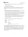
5) Click on Problem Definition Tab, within Decision Variable File section, click on Browse button to
browse to the following folder:
C:\DarwinWorkshop\Examples\SingleObjective
6) Load the file DecisionVariables.txt from the folder as shown below.
8
Darwin Optimization
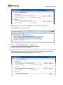
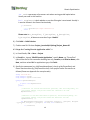
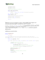
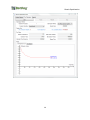
7) Within Configuration section, Click on Edit button, it opens the configuration file
Configuration.xml in Notepad as follows.
8)
Replace “Your\Path\To\FitnessDLL” as highlighted with
“C:\DarwinWorkshop\Examples\SingleObjective\Fitness.dll”
9) Save the configuration file and close the file.
10) By default, Output Directory is set to your local user folder. To change it, click on Change button
within Output Directory section, it will allow you to change the output folder as desired, e.g.
C:\DarwinWorkshop\Examples\SingleObjective, as shown below.
9
Darwin Optimization
11) Click on Run Optimization tab, and then simply click on Start button to make a run. At the run
time, you can pause by click on Pause button, resume the run by clicking on Resume button, or
stop the run by clicking on Stop button.
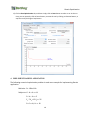
4. IMPLEMENT DARWIN APPLICATION
The following numerical optimization problem is used as an example for implementing Darwin
application.
Minimize: O1: 10X0+11X1
Subject to: C1: X0 + X1 >= 11
C2: X0 – X1 <= 5
C3: 7 X0 + 12 X1 >= 35
C4: 0 <= X0, X1 <= 10
10
Darwin Optimization
Decision file (decisionTest.txt) is created to define the options for the optimization variables as
follows.
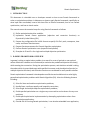
4.1. Define Decision Variables
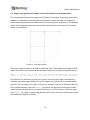
Optimization variables are specified in a text file. It follows the format as in figure below.
Definition of optimization variables
Decision variables are defined with a header [DECISIONVARIABLES] and followed by
minimum, maximum and increment for each variable. Darwin optimization is to search for
the near-optimal value in between the upper and lower limits with the specified increment.
The file can be named as Decision.txt or any desired name. It is suggested that the file be
saved in the same folder as Output Directory.
The primary task for developing and prototyping Darwin optimization application is to
implement the objective and constraint functions. The implementation can proceed with C#
and C++.
4.2. Steps for Creating Darwin Application with C#
1) In Microsoft Visual Studio, File -> New -> Project
2) In Visual C#, under Windows, choose “Class Library”, specify Name e.g. “FitnessTest”
(this will be the DLL file name after building later on), Location, and Solution Name, click
OK.
3) Fitness function must be specified as the prototype as follows.
int MyFitnessFuntion(ArrayList, ArrayList, ArrayList, ArrayList, int, bool)
4) Specify the namespace (e.g. MyFitnessNameSpace), class (e.g. MyFitnessClass) and
fitness function name (e.g. MyFitnessFunction). Your project source file contains as
follows.
using System;
using System.Collections;
namespace MyFitnessNameSpace
11
Darwin Optimization
{
public class MyFitnessClass
{
#region Fitness Calculation method
public int MyFitnessFunction(ArrayList x_ArrayList, ArrayList f_ArrayList,
ArrayList g_ArrayList, ArrayList h_ArrayList, int rank, bool terminated)
{
//TODO your implementation; example code is provided in section 6.1
//Alternatively, the code in section 6.1 or from file FitnessCodes.cs can be
//copied and pasted here
return 1;
}
#endregion
}
}
5) Implement fitness function as follows (Please see the sample code Section 6).
a. Definition of fitness function
Following the example is provided with Darwin optimization framework, the
definition of the fitness function is as follows.
public int MyFitnessFunction(ArrayList x_ArrayList, ArrayList
f_ArrayList, ArrayList g_ArrayList, ArrayList h_ArrayList, int
rank, bool terminated)
b. Parameters and return value of fitness function
ArrayList x_ArrayList: current solution (decision variable values) passed
from Darwin Framework. The size of x_ArrayList is the same as the number of
variables in the decision file.
ArrayList f_ArrayList: store objective function value(s) to be calculated for
the current solution stored in x_ArrayList. After objective value is calculated for
the solution, it is added to f_ArrayList, which returns it to Darwin Framework.
The size of the f_ArrayList is the same as the number of objective function(s).
ArrayList g_ArrayList: store the violation of inequality constraint functions,
which are calculated for the current solution (decision values) in x_ArrayList.
The violation is added to g_ArrayList, which returns the violation to Darwin
Framework. The size of the g_ArrayList is the same as the number of inequality
constraint functions. Value of 0 indicates the constraint is satisfied. The larger the
values, the worse violated the current trial solution is.
ArrayList h_ArrayList: store the violation of equality constraint functions,
which are calculated for the current solution in x_ArrayList. The violation is
added to h_ArrayList, which return the violation to Darwin Framework.
12
Darwin Optimization
int rank: a parameter of processor rank when running parallel optimizaiton.
Usually not used in this function.
bool terminated: check whether or not the GA engine is terminated. Usually it
is used as follows in the fitness function body.
if (terminated)
{
Console.WriteLine("GA engine terminated.");
return 1;
}
Please note: In x_ArrayList, f_ArrayList, g_ArrayList,
h_ArrayList, all elements must be of type “double”.
6) Click Build -> Build Solution
7) Find the new DLL file here: Project_Location\bin\Debug\Project_Name.dll
4.3. Steps for Creating Darwin Application with C++
1) In Visual Studio, File -> New -> Project
2) In Visual C++, choose “Win32 Console Application”, specify Name e.g. “FitnessTest”
(this will be the DLL file name after building later on), Location, and Solution Name, click
Next, and then select DLL for application type, click Finish.
3) Specify the namespace (e.g. MyFitnessNameSpace), class (e.g. MyFitnessClass) and
fitness function name (e.g. MyFitnessFunction). Your project source file contains as
follows (Please see Appendix for a sample code).
#using <mscorlib.dll>
using namespace System;
using namespace System::Collections;
namespace MyFitnessNameSpace
{
__gc public class MyFitnessClass
{
public:
//constructor for one-time initialization operations, like allocating memory, etc.
//in parallel running, each process invokes the constructor one time.
MyFitnessClass() { }
//destructor for one-time finialization operations, like delocating memory, etc.
//in parallel running, each process invokes the destructor one time.
~MyFitnessClass() { }
int MyFitnessFunction(ArrayList * x_ArrayList, ArrayList * f_ArrayList, ArrayList
* g_ArrayList, ArrayList * h_ArrayList, int rank, bool terminated)
{
if (terminated)
13
Darwin Optimization
{
Console::WriteLine("GA engine terminated.");
return 0;
}
//TODO your implementation
return 1;
}
};
}
4) Right click the project in the Solution Explorer, choose Property to open property
pages.
5) Configuration Properties -> General, in Configuration Type choose Dynamic Library
(.dll) in the dropdown menu, and in Common Language Runtime support choose
Common Language Runtime Support, Old Syntax (/clr:oldSyntax).
6) Click Build -> Build Solution.
7) Find the new DLL file here: Project_Location\Debug\Project_Name.dll
5. RUN DARWIN OPTIMIZATION
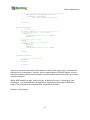
5.1. Prepare Darwin Configuration File
Darwin configuration file is a XML file for specifying the path of the application fitness
DLL file as well as the namespace, class name and fitness function name. Darwin
framework uses “Configuration.xml” (please note this file name is fixed) file to locate
the fitness function DLL and exact fitness function for the run. For a new application,
you can edit the sample configuration file with corresponding path, name space, class
name and fitness function name, and save the edited file in the same folder as decision
variable file. A sample Configuration.xml file is shown below.
The above sample shows that the fitness function is named “MyFitnessFunction” as a method
of class “MyFitnessClass”, under namespace “MyFitnessNameSpace”, and in the file of
“C:\DarwinWorkshop\Examples\SingleObjective\Bentley.Darwin.Fitness.dll”.
14
Darwin Optimization
Before running Darwin, make sure that (1) fitness DLL file is created for the application; (2)
decision file (.txt) is created for the runs and (3) configuration file is edited and saved in the
same folder as decision.
5.2. Run Darwin
Using GUI, simply click on the desktop icon
. Basic steps for running Darwin are below.
Click on Problem Definition tab, and
1) Load decision variable file;
2) Load configuration file;
3) Change the output folder as desired.
Click on Run Optimization tab
After decision variable file and configuration files are loaded, the problem information,
including No. of Decision Variables, No. of Objectives and No. of Possible solutions, is calculated
and displayed within the section of Problem Size.
You can run Darwin in sequential optimization when Number of Process is 1 or in parallel
optimization when Number of Process is greater than 1. Choose the desired optimization
method and constraint handling technique, click on Start button to run Darwin. To pause the
run, click on Pause button, to resume the run, click on Resume button. To terminate the run,
click on Stop button.
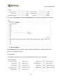
Darwin run time status is updated during the run as below.
15
Darwin Optimization
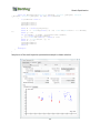
The results of Convergence Curve and Top Solutions are also dynamically updated as follows.
5.3 Darwin Options
Under Options tab, three sections of data including GA Parameters, Stopping Criteria and
Options, are specified as below.
GA Parameters
If simple GA is selected for the run, the following GA parameters are used below.
16
Darwin Optimization
If the fmGA is selected for the run, the GA parameters are as follows.
Hot Start with Exported Template: if checked, the best chromosome exported from previous
run using fmGA will be used as template for the current run. The template serves as hot start
and speed up the convergence to the near optimal solutions.
Stopping Criteria
1) Maximum Running Time: Darwin run will be terminated after the specified time is used
up.
2) Maximum Trials: Darwin run will be terminated after reaching the maximum number of
trial solutions.
3) Max Non Improve Gens: Darwin run will be terminated if the best solution is not
improved after the maximum number of non-improvement generations.
4) Maximum Generations: If simple GA is used, Darwin will be terminated if the number of
generation reaches the maximum generations.
Options
17
Darwin Optimization
1) Top Solution to Keep: specify the number of near-optimal solutions to save for the single
objective optimization. For Multi-objective solution, all Pareto solutions are saved for
the run.
2) Random Seed: specify the seed for generating initial population of solution.
3) Save a Batch File: if checked, a batch file will be created to run Darwin in console
prompt. Simply click the batch file to run Darwin in Console. A sample batch file for
parallel optimization run is created and listed below.
@echo off
mpiexec.exe -n 3 C:\PROGRA~2\Bentley\DARWIN~1\Bin\Bentley.Darwin.Console.exe FastMessyGA
C:\DARWIN~1\Examples\SINGLE~1\DECISI~1.TXT C:\Users\zheng.wu\AppData\Local\DARWIN~2\GA_parameters.txt violation
C:\Users\zheng.wu\AppData\Local\DARWIN~2\TopSolution.txt
pause
5.4 Start Darwin Using Command
Apart from running Darwin in console using batch file created by GUI, in general, Darwin can be
run with the following command and arguments.
1) Start Darwin GUI using command line:
Open console prompt and change directory to the folder where decision variable file
and configuration file are located, use the following command to start Darwin GUI:
[Darwin bin path]\Bentley.Darwin.GUI2.exe decision_file.txt
C:\PROGRA~2\Bentley\DARWIN~1\Bin\Bentley.Darwin.GUI2.exe C:\DARWIN~1\Examples\SINGLE~1\DECISI~1.TXT
2) Sequential optimization run command (use the same folder with .exe to eliminate
[path+]):
Bentley.Darwin.Console.exe type_of_GA [path+]decision_file.txt
[path+]parameter_file.txt [type_of_constrant_handling_method] [path+]log_file.txt
3) Parallel optimization command (use the same folder with .exe to eliminate [path+]):
Mpiexec –n 4 Bentley.Darwin.Console.exe type_of_GA [path+]decision_file.txt
[path+]parameter_file.txt [type_of_constrant_handling_method]
[path+]TopSolution_file.txt
a. MPI should be installed and is need to start the parallel application.
b. type_of_GA: “FastMessyGA” for fast messy Genetic Algorithm; “SimpleGA” for
simple Genetic Algorithm.
18
Darwin Optimization
c.
Constraint handling methods. For “FastMessyGA”, two methods are available
for handling constraints, “penalty” or “violation”. For “SimpleGA”, this argument
is eliminated, which uses “penalty” to handle constraints.
d. TopSolution_file.txt: result file that contains the top solutions found by Darwin
optimization engine.
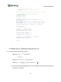
5.5 Debug Darwin Applications
It is important to be able to debug the fitness implementation. In order to do so, Darwin needs
to be launched in console. Simply add DEBUG to the end of command line or in the batch file,
such as:
When running Darwin in console with DEBUG argument, the run process will pause as below.
Darwin run process can be then attached with the fitness project for debugging.
6. EXAMPLES
6.1. Single Objective Optimization Fitness Code (C#)
using System;
using System.Collections;
namespace MyFitnessNameSpace
{
public class MyFitnessClass
{
//constructor for one-time initialization operations, like allocating memory, etc.
//in parallel running, each process invokes the constructor one time.
MyFitnessClass() { }
//destructor for one-time finialization operations, like delocating memory, etc.
//in parallel running, each process invokes the destructor one time.
~MyFitnessClass() { }
#region Fitness Calculation method
public int MyFitnessFunction(ArrayList x_ArrayList, ArrayList f_ArrayList,
ArrayList g_ArrayList, ArrayList h_ArrayList, int rank, bool terminated)
19
Darwin Optimization
{
if (terminated)
{
Console.WriteLine("GA engine terminated.");
return 0;
}
//Console.WriteLine("x_ArrayList come form rank = " + rank);
//TODO: Implement the function- User defined
f_ArrayList.Clear();
g_ArrayList.Clear();
h_ArrayList.Clear();
/* objective function */
f_ArrayList.Add(10.0 * (double)x_ArrayList[0] + 11.0 *
(double)x_ArrayList[1]);
double g_value;
/* constraints g<=0 */
g_value = 11 - ((double)x_ArrayList[0] + (double)x_ArrayList[1]);
if (g_value <= 0) g_value = 0;
g_ArrayList.Add(g_value);
g_value = (double)x_ArrayList[0] - (double)x_ArrayList[1] - 5;
if (g_value <= 0) g_value = 0;
g_ArrayList.Add(g_value);
g_value = 35 - (7.0 * (double)x_ArrayList[0] + 12.0 *
(double)x_ArrayList[1]);
if (g_value <= 0) g_value = 0;
g_ArrayList.Add(g_value);
return 1;
}
#endregion
}
}
6.2. Single Objective Optimization Fitness Code (C++)
#using <mscorlib.dll>
using namespace System;
using namespace System::Collections;
namespace MyFitnessNameSpace
{
__gc public class MyFitnessClass
{
public:
//constructor for one-time initialization operations, like allocating memory, etc.
//in parallel running, each process invokes the constructor one time.
MyFitnessClass() { }
//destructor for one-time finialization operations, like delocating memory, etc.
//in parallel running, each process invokes the destructor one time.
~MyFitnessClass() { }
int MyFitnessFunction(ArrayList * x_ArrayList, ArrayList * f_ArrayList, ArrayList
* g_ArrayList, ArrayList * h_ArrayList, int rank, bool terminated)
{
if (terminated)
{
20
Darwin Optimization
Console::WriteLine("GA engine terminated.");
return 0;
}
//Console.WriteLine("x_ArrayList come form rank = " + rank);
//TODO: Implement the function- User defined
f_ArrayList->Clear();
g_ArrayList->Clear();
h_ArrayList->Clear();
/* objective function */
IEnumerator * temp = x_ArrayList->GetEnumerator(0,2);
temp ->MoveNext();
double tempx0 = *dynamic_cast<__box Double*>(temp->Current);
temp ->MoveNext();
double tempx1 = *dynamic_cast<__box Double*>(temp->Current);
f_ArrayList->Add(__box(10.0 * tempx0 + 11.0 * tempx1));
double g_value;
/* constraints g<=0 */
g_value = 11 - (tempx0 + tempx1);
if (g_value <= 0) g_value = 0;
g_ArrayList->Add(__box(g_value));
g_value = tempx0 - tempx1 - 5;
if (g_value <= 0) g_value = 0;
g_ArrayList->Add(__box(g_value));
g_value = 35 - (7.0 * tempx0 + 12.0 * tempx1);
if (g_value <= 0) g_value = 0;
g_ArrayList->Add(__box(g_value));
return 1;
}
};
}
6.3. Multiple Objective Optimization (using fast messy GA)
This example problem is formulated as follows.
Minimize:
:
:g*h
Subject to:
Where:
, and
.
1) Create decision file (MultiOjbDecision.txt) of variables to be determined and capture
constraint C4 as follows:
21
Darwin Optimization
2) Create new DLL file of the fitness as stated in the section of Implement Darwin
Fitness Application. C# sample codes are in the next section.
3) Create “Configuration.xml” file as follows (it is recommended to move the decision
file, parameter file, and DLL file to a folder of convenience before this step). Replace
[PathToDLLFile\] accordingly.
<?xml version="1.0" encoding="UTF-8" ?>
<FitnessDLLConfiguration>
<FitnessDllFilePath>[PathToDLLFile\]MultiObjFitness.dll</FitnessDllFilePath>
<FitnessDllNamespace>MyFitnessNameSpace</FitnessDllNamespace>
<FitnessDllClassName>MyFitnessClass</FitnessDllClassName>
<FitnessFunctionName>MultiObjective</FitnessFunctionName>
</FitnessDLLConfiguration>
4) Place “Configuration.xml” under the same folder as the decision variable file.
5) Start Darwin, load the corresponding decision file and configuration file, and make
sure to select Fast Messy Genetic Algorithm for the run.
6) Top (Pareto) solutions will be plotted at run time and also saved in the
TopSolutions.txt.
The C# code for this example is listed below.
using
using
using
using
System;
System.Collections;
System.Linq;
System.Text;
namespace MyFitnessNameSpace
{
public class MyFitnessClass
{
#region Fitness Calculation method
22
Darwin Optimization
public int MultiObjective(ArrayList x_ArrayList, ArrayList f_ArrayList, ArrayList
g_ArrayList, ArrayList h_ArrayList, int rank, bool terminated)
{
if (terminated) return 1;
f_ArrayList.Clear();
g_ArrayList.Clear();
h_ArrayList.Clear();
double x1 = (double)x_ArrayList[0];
double f1 = 1 - Math.Exp((double)(-4) * x1) * Math.Pow(Math.Sin(x1 * 6 * 3.1415926),
6);
double g = 0.0F;
for (int nIndex = 1; nIndex < x_ArrayList.Count; nIndex++)
g += (double)x_ArrayList[nIndex];
g = 1 + 9 * Math.Pow((double)g / (double)9, 0.25);
double h = 1 - Math.Pow((f1 / g), 2);
double f2 = g * h;
f_ArrayList.Add(f1);
f_ArrayList.Add(f2);
return 1;
}
#endregion
}
}
Sample run of the multi objective optimization example is shown as below.
23
Darwin Optimization
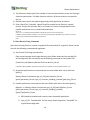
6.4. Engineering Application Example: Water Distribution System Optimization
This example demonstrates then application of Darwin to solving an engineering optimization
problem. It is specified to optimize pipe sizes (diameters) so that the total cost of design is
minimized and the pressures at nodes meet the minimum pressure requirement. The example
system used is Twoloop network the benchmark example used in the literature. The system
layout is shown below.
Layout of Twoloop Network
The system contains 8 pipes to be sized or optimized, each of the 8 pipes with length of 1000
meters can take a size from the available possible diameters (14 of them) as specified below.
diam[]
= {25.4,50.8,76.2,101.6,152.4,203.2,254.0,304.8,355.6,406.4,457.2,508.0,558.8,609.0};
unitcost[] = {2.0, 5.0, 8.0,11.0, 16.0, 23.0, 32.0, 50.0, 60.0, 90.0, 130.0,170.0, 300.0,550.0};
The objective is to minimize the total cost of pipes. The cost for each pipe is calculated by
multiplying the pipe length (1000) with the unit-length cost ($/meter) for the corresponding
pipe size. The unit-length cost is given in unitcost[ ] as above. Each pipe is allowed to take any
of 14 possible diameter sizes from diam[]. To optimize the pipe sizes, the diameter index is
used as decision variable, which can take a value from 0 to 13, for instance, 0 diameter index
from diam[] for a pipe is representing diameter of 25.4 mm. Therefore, the decision variable
file is defined for 8 pipes as follows.
24
Darwin Optimization
The constraint for this example is to satisfy the minimum pressure head of 30.0 meters at the
junctions (6 of them). EPANET2 toolkit is used for the implementation. The toolkit contains a set
of APIs for executing analysis runs, updating and retrieving model attributes.
As installed with Darwin, this example is implemented in WDSOptimizaiton solution, which
contains two projects, including WDSFitness and WDSEvaluation.
WDSFitness project is implemented as follows.
#using <mscorlib.dll>
#include "interface.h"
using namespace System;
using namespace System::Collections;
using namespace System::Runtime::InteropServices;
namespace MyFitnessNameSpace
{
__gc public class MyFitnessClass
{
public:
MyFitnessClass()
{
OpenEngine();
}
~MyFitnessClass()
{
//close epanet engine
CloseEngine();
}
int TwoLoopFitnessFunction(ArrayList * x_ArrayList, ArrayList * f_ArrayList, ArrayList *
g_ArrayList, ArrayList * h_ArrayList, int rank, bool terminated)
{
if (terminated)
{
Console::WriteLine("Darwin is terminated.");
return 0;
}
// clear array lists
25
Darwin Optimization
f_ArrayList->Clear();
g_ArrayList->Clear();
h_ArrayList->Clear();
//preparing new solution for evaluation
int nx = x_ArrayList->Count;
Int32 index[] = new Int32[nx];
for(int i=0;i<nx;++i)
index[i] = *dynamic_cast<__box double*>(x_ArrayList->get_Item(i));
int __pin* xList = &index[0];
double violation = 0.0;
double totalcost = 0.0;
objFunction(xList,nx,&violation,&totalcost);
f_ArrayList->Add(__box(totalcost));
g_ArrayList->Add(__box(violation));
return 1;
}
}
}
WDSFitness is set up as a managed C++ project. It opens EPANET analysis engine in the
constructor and close the engine in the destructor. The fitness function
TwoLoopFitnessFunction(ArrayList * x_ArrayList, ArrayList * f_ArrayList, ArrayList * g_ArrayList,
ArrayList * h_ArrayList, int rank, bool terminated)
is implemented to receive the new solution
from Darwin and evaluate it in the function objFunction(xList,nx,&violation,&totalcost)
, which is implemented along with OpenEngine() and CloseEngine() in the C/C++ project of
WDSEvaluation.
WDSEvaluation.cpp code is below.
#define LPLIBRARY_EXPORT
#include "interface.h"
#include "epanet2.h"
float diam[] =
{25.4,50.8,76.2,101.6,152.4,203.2,254.0,304.8,355.6,406.4,457.2,508.0,558.8,609.0};
float unitcost[] = {2.0, 5.0, 8.0,11.0, 16.0, 23.0, 32.0, 50.0, 60.0, 90.0, 130.0,170.0,
300.0,550.0};
static float pipelength = 1000.0;
static float minpressure = 30.0;
double LPAPI objFunction(int *xList, int xListSize, double *violation, double *objvalue)
{
//calculate cost objective function;
*objvalue = 0.0;
for (int i = 0; i < xListSize; i++){
*objvalue +=pipelength*unitcost[xList[i]];
int linkindex = i+1;
//set new diameters (new solution) to the analysis engine
ENsetlinkvalue(linkindex, EN_DIAMETER,diam[xList[i]]);
};
//run epanet analysis engine
ENsetstatusreport(0);
ENsetreport("MESSAGES NO");
ENinitH(0);
ENsolveH();
//check constraint(nodal pressure) violation
float pressure;
*violation = 0.0;
26
Darwin Optimization
for (int i = 1; i <= 6; i++){ //6 junctions in twoloop model
ENgetnodevalue(i, EN_PRESSURE, &pressure);
if (pressure < minpressure){
*violation += minpressure - pressure;
};
};
return(1.0);
}
int LPAPI OpenEngine()
{
// open model files
int errNum = ENopen("twoloop.inp", "twoloop.rpt", "");
//printf("ENopen errNum = %d \n", errNum);
if (errNum != 0){
printf("ENopen errNum = %d \n", errNum);
ENclose();
};
//open epanet analysis solver
ENopenH();
//printf("\n openH err = %i", errNum);
if (errNum != 0){
ENcloseH();
ENclose();
printf("ENopen errNum = %d \n", errNum);
};
return(1);
}
int LPAPI CloseEngine()
{
//close epanet analysis engine
ENcloseH();
ENclose();
return(1);
}
objFunction( ) receives new solution (new diameter index for each pipe) in xList, calculates the
total pipe cost ( as assigned to *objvalue), sets the new diameters to EPANET engine, runs the
hydraulic simulation with the new diameters, retrieves nodal pressure and checks for pressure
constraint violation.
Within WDSEvaluation project, three functions, including objFunction( ) , OpenEngine( ) and
CloseEngine( ) are implemednted and published or exported for being used in WDSFitness
project. The prototype of the published APIs is specified in interface.h.
Interface.h code is below.
27
Darwin Optimization
#pragma once
#if defined(LPLIBRARY_EXPORT) // inside DLL
#
define LPAPI
__declspec(dllexport)
#else // outside DLL
#
define LPAPI
__declspec(dllimport)
#endif // LPLIBRARY_EXPORT
#include <stdio.h>
extern "C"{
double LPAPI objFunction(int *,int, double *, double *);
int LPAPI OpenEngine();
int LPAPI CloseEngine();
}
To run this example, follow the steps below:
1) Open MS VS (2008 or newer version), and load the solution WDSOptimization from
folder C:\DarwinWorkshop\Examples\WDSOptimization (or the folder where the
Examples are copied to).
2) Click on Build->Build Solution, the solution will be built with two DLLs created in folder
..\Examples\WDSOptimization\Release, or debug folder if build in debug mode.
3) Copy WDSEvalution.dll and WDSFitness.dll into C:\DarwinWorkshop
\Examples\WDSObjective
4) Click Darwin icon on desktop to start Darwin.
5) Load decision variable file TwoloopDecisionVariables.txt from
C:\DarwinWorkshop\Examples\WDSObjective, the configuration file in the same folder
will be automatically loaded, make sure the path and fitness dll file name are correct.
6) Change the output folder as desired, then you can run the application as shown below.
28
Darwin Optimization
29
Darwin Optimization
TECHNIQUE REFERENCE: DARWIN OPTIMIZATION METHOD
The framework encapsulates the core methodology for solving single and multiple objective
optimization problems, the techniques for handling equality and inequality constraints, and also
provides the options for executing solution evaluation/fitness in multiple processes as needed. It
decouples the parallel optimization solver from domain applications and enables rapid implementation
of infrastructure optimization projects with thin-client architecture. The parallel optimization is based on
the competent genetic algorithm that has successfully applied to water distribution optimization
problems including model calibration, network design and pump scheduling. The framework has
recently been applied to geometry design optimization, building energy performance-based design
optimization, finite element analysis model updating (calibration) and damage detection for civil
infrastructure health monitoring (Wu, Wang, Butala, & Mi, 2011) [1]. The generalized Darwin framework
contains both simple GA and fast messy GA as optimization solvers.
6.5. Simple Genetic Algorithm
A genetic algorithm is a search method that emulates the principles of genetic reproduction operations
such as crossover and mutation. It is a branch of evolutionary computation and formally introduced by
Holland in 1975 (Holland 1975) [2]. Since then, genetic algorithm has been one of the most active
research fields in artificial intelligence. Many successful applications have been made in engineering,
science, economy, finance, business and management. There are many variations of GA, but basic idea is
as follows.
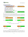
GA represents a solution as a string, for instance a binary string as shown in Figure 7.1. It can be any
other type of strings. The string is referred to as phenotype or chromosome. One segment of string is
assigned to represent one decision variable (e.g. one leak) and thus one completed solution (e.g. a
number of leaks for a water distribution system) is encoded onto one string as shown in Figure 7.1.
Figure 7.1 An example of genetic algorithm solution representation
Initially, a population of strings or solutions is randomly created. Each of the solutions is evaluated by
performing the corresponding hydraulic simulation (either steady state or transient analysis). A fitness
value can be calculated by the objective function and assigned to the solution or string. By emulating the
principle of Darwin’s survival-of-fittest, the better solution is selected as parent to reproduce next
generation of solution. Figure 7.2 illustrates operation of selecting two parents.
30
Darwin Optimization
Figure 7.2 Example GA population solutions and selection operation
The selected parent strings are to reproduce offspring namely the child solutions. Two operations of
crossover and mutation are mimicked for the reproduction. As shown in Figure 7.3, crossover is to first
cut two strings at a randomly selected crossover point and then exchanges partial chromosomes to form
two new child solutions.
Figure 7.3 Genetic algorithm crossover operations
Figure 7.4 Genetic algorithm mutation operations
After crossover, a new solution may be mutated by changing the bit value. As illustrated in Figure 7.4, a
bit may be selected as highlights and its value is flipped from 0 to 1 (or1 to 0). Both crossover and
mutation are applied by performing a probabilistic test and when its probability is greater than the
31
Darwin Optimization
prescribed probability. Repetitively applying selection, crossover and mutation, a new population of
solutions can be reproduced, and each of them is evaluated with a fitness value. This far, one generation
is completed. Generation after generation, the population of strings are expected to evolve to optimal
or near-optimal solution.
This is the basic procedure of simple GA. There are different variations based on the principles of the
simple genetic algorithm. The improvement of the existing GA methods and new GAs have been
constantly developed and reported in literature every year. Overall, many advantages are identified for
GA search for good solutions (Goldberg 1989). The primary merit is its capability of solving nonlinear
optimization problems. Model-based leakage detection is a typical implicit nonlinear optimization
problem.
6.6. Fast Messy Genetic Algorithm Key Features
Similar to simple GA, but fast messy GA (fmGA) is different with the key features including flexible string
length, gene filtering and multi-era search process. It is originally developed as one of the competent
genetic algorithms (Goldberg 2001) [3] for solving the hard-problems more efficiently and effectively.
With fmGA, a flexible scheme is employed to represent a calibration solution with strings
(chromosomes) of variable lengths. The length of strings changes from one string to another. Short
strings namely partial solutions are generated and evaluated during the early stage of GA optimization.
The short strings with better fitness value above the average are considered to retain “building blocks”
that form the good solutions. The fmGA starts with an initial population of full-length strings and follows
by a building block filtering process. It identifies the better fit short strings by randomly deleting genes
from the initial strings. The identified short strings are used to generate new solutions. A solution is
formed by “cut” and “splice” operations instead of standard GA crossover. “Cut” divides one string into
two strings while “splice” link two strings to create one individual string. Both genetic operations are
purposely designed to effectively exchange the building blocks for generating good solutions.
The fmGA combines building block identification and solution reproduction phases into one artificial
evolution process and proceeds over a number of outer iterations or so-called eras. Each era consists of
solution initialization, building block filtering and reproduction. The eras continue until good solutions
are found or computation resources reach the maximum limit. The fmGA is employed as a competent
optimizer for evolving effective water distribution models and embedded into a multi-tier modeling
software System (Bentley 2006 [4] and Haestad 2002 [5]).
6.7. Parallelism Paradigms
The software world has been very active part of the evolution of parallel computing. As multi-core
processors bring parallel computing to mainstream customers, the key challenge in computing today is
to transition the software industry to parallel programming. Parallel programs have been harder to write
than sequential ones. A program that is divided into multiple concurrent tasks is more difficult to
32
Darwin Optimization
implement, due to the necessary synchronization and communication that needs to take place between
those tasks. Some standards have emerged. There are two types of computation parallelism at
instruction level, data parallelism and task parallelism. Both data and task parallelisms can be achieved
by different programming languages, libraries and application programming interfaces (APIs). Message
passing interface (MPI) [6] and Open Multi-Processor (OpenMP) [7] are among the most commonly-used
libraries for task parallelism and data parallelism.
6.7.1. Task parallelism
Task parallelism is a parallel computing program that a computing problem is divided into many
computing tasks and that different calculations can be performed on different computing processes
(CPUs or nodes). Each of the computing tasks can be performed with either the same or different sets of
data. Task parallelism usually scales with the number of computing nodes. There are various methods
for achieving task parallelism computing, a message passing communication is usually employed for a
scalable and portable implementation.
Message Passing Interface is a specification of the application programming interface (API) that allows
many computers to communicate with one another. It is used for parallelizing computing task over a
cluster of machines or on supercomputers, where each of the CPU is representing a computing node or
process. It is a language-independent communications protocol supporting both point-to-point and
collective communication. MPI is designed for developing high performance computing applications
with scalability and portability. It is one of the popular models used in high-performance computing.
MPI consists of more than 115 functions [8]. Various MPI implementations are as follows.
1) DeinoMPI [9] is an implementation of MPI-2 for Microsoft Windows. This is the release version
1.1.0 with downloads for both Win32 and Win64 machines.
2) PureMPI.NET [10] is a completely managed implementation of the message passing
interface. The object-oriented API is simple, and easy to use for parallel programming. It has
been developed based on the latest .NET technologies, including Windows Communication
Foundation (WCF). This allows you to declaratively specify the binding and endpoint
configuration for your environment, and performance needs. When using the SDK, a
programmer will definitely see the MPI'ness of the interfaces come through, and will enjoy
taking full advantage of .NET features - including generics, delegates, asynchronous results,
exception handling, and extensibility points.
3) MPI.NET [11] is a high-performance, easy-to-use implementation of the Message Passing
Interface (MPI) for Microsoft's .NET environment. MPI is the de facto standard for writing
parallel programs running on a distributed memory system, such as a compute cluster, and is
widely implemented. Most MPI implementations provide support for writing MPI programs in C,
C++, and FORTRAN. MPI.NET provides support for all of the .NET languages (especially C#), and
includes significant extensions (such as automatic serialization of objects) that make it far easier
to build parallel programs that run on clusters.
4) MPICH2 is a high-performance and widely portable implementation of the Message Passing
Interface (MPI) standard (both MPI-1 and MPI-2). The goals of MPICH2 is to provide an MPI
33
Darwin Optimization
implementation that efficiently supports different computation and communication platforms
including commodity clusters, high-speed networks and proprietary high-end computing
systems.
5) MSMPI [12] is the Microsoft’s implementation of MPICH2 for Windows Compute Cluster Server
and High Performance Computing Server [13].
6.7.2.
Data parallelism
Data parallelism is inherent in program loops, which focuses on distributing the data across different
computing nodes to be processed in parallel. Parallelizing loops often leads to similar operation
sequences or functions being performed on elements of a large data structure. Many scientific and
engineering applications exhibit data parallelism. The most commonly adopted programming language
for data parallelism is Open Multi-Processors (OpenMP).
The OpenMP is a set of APIs that support multi-platform shared memory multiprocessing programming
in C/C++ and FORTRAN on UNIX and Microsoft Windows platforms. It consists of a set of compiler
directives, library routines, and environment variables that influence run-time behaviour. Jointly defined
by a group of major computer hardware and software vendors, OpenMP is a portable, scalable model
that gives programmers a simple and flexible interface for developing parallel applications for platforms
ranging from the desktop to the supercomputer. An application built with the hybrid model of parallel
programming can run on a computer cluster using both OpenMP and Message Passing Interface (MPI).
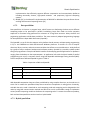
A brief comparison of MPI and OpenMP is given in Table 1.
Table 1 Comparison of MPI and OpenMP
Criteria
OpenMP
MPI
Platform
Symmetric Multiprocessing(SMP)
Both SMP and Clusters
Parallelism
Fine grain parallelism
Coarse grain parallelism
Performance
Better on SMP
Better on Cluster
With OpenMP computation loops are often parallelized by using compiler directives, so the code runs in
serial until it reaches the parallelized loop where concurrent computation is taking place. Conversely,
with MPI the entire code is launched on each computing node and computing task is designated to the
node by using MPI communication methods and APIs that are rich and flexible enough to implement
various parallel computing models to distribute the computing tasks. To ensure the maximum speedup,
both task and data parallelism can be mixed in a hybrid model.
6.7.3. Hybrid parallelism
34
Darwin Optimization
A hybrid parallelism is to implement both task and data parallel computation in the same application to
obtain the maximum speedup. A number of hybrid computation models [14] have been compared and
summarized as follows.
1) Pure MPI: Task and data parallelisms are achieved by just using MPI library. The
communications within one task process and across multiple task processes are implemented
as a flat massively parallel processing (MPP) system.
2) MPI and OpenMP: Task parallelism is implemented by calling MPI communication methods
across several computing nodes. Within each parallel task process, OpenMP is used for data
parallelism.
3) Pure OpenMP: Based on virtual distributed shared memory systems (DSM), the application is
parallelized only with shared memory directives of OpenMP.
The hybrid parallelism models offer advantages for the clusters of SMP computing nodes, but have some
serious disadvantages based on mismatch problems between the hybrid programming scheme and the
hybrid architecture, including:
1) With pure MPI, minimizing the inter-node communication requires that the applicationdomain’s neighborhood-topology matches with the hardware technology. Otherwise, more data
is shipped over the inner-node network instead of using the shared memory based
communication within nodes. On the other hand, Pure MPI also introduces intra-node
communication on the SMP nodes that can be omitted with hybrid programming.
2) With MPI and OpenMP programming, the intra-node communication overhead, introduced by
pure MPI method, can be substitute by direct access to the application data structure in the
shared memory. However, this programming style is not able to achieve full inter-node
bandwidth on all platforms for any subset of inter-communicating threads. For instance, with
manager only style, all non-communicating threads are idling. CPU time is also wasted, if all
CPUs are already able to saturate the inter-node bandwidth. With hybrid manager only
programming, additional overhead is induced by all OpenMP synchronization, but also by
additional cache flushing between the generation of data in parallel regions and the
consumption in subsequent message passing routines and calculations in subsequent parallel
sections.
3) Overlapping of communication and computation is a chance for an optimal usage of the
hardware, but it causes serious programming effort in the application itself, in OpenMP
parallelization and load balancing.
4) Although pure OpenMP is simple and runs efficiently in shared-memory multiprocessor
platforms, its scalability is limited by memory architecture.
Different programming schemes on clusters of SMPs show different performance benefits or penalties
on the hardware platform. In order to obtain the best performance results, we have to choose the
schemes bases on both the hardware and computer algorithm. In the project of pump scheduling
optimization, we choose the latest release of MPICH2 as our parallel computation interface. It is also
readily compatible with MSMPI supported by Microsoft Window Server 2008 and its High Performance
Computing Server.
6.8. Darwin Optimization Architecture
35
Darwin Optimization
Darwin optimization framework is based on fast messy Genetic Algorithm (fmGA) [15], [16] solver, which
has been developed and applied to a number of optimization modeling tools including Darwin Calibrator
[17], Darwin Designer [18] and Darwin Scheduler [19] for water distribution optimization. These
applications employ the same solver of fmGA and share the similar architecture. fmGA optimization
solver is decoupled from the specific applications and developed as a generic, scalable and extensible
optimization solver. The common optimization solver is further generalized and implemented as parallel
optimization framework.
The optimization framework is developed to meet the following criteria.
1) Generic Framework: The framework provides an architecture which has a strong decoupling
between the problem definition and the framework. The framework can be used to solve any
optimization problem.
2) Parallel Architecture: The framework provides application independent from the parallel
optimization framework. All the parallel computation is done inside the framework. User needs
minimum knowledge about parallel computing.
3) Framework User Interface: In addition a generic parallel framework, it also has a generic user
interface which allows a user to set all the optimization controls. The user interface also
provides a runtime optimization updates to the user.
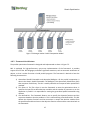
6.8.1. Parallel computation model
A manager/worker model, as shown in Figure 7.5, is implemented for parallel genetic optimization. After
GA initialization, manager process sends chromosomes to worker processes where EPS and fitness
calculation is performed for solution evaluation. Then manager process collects the fitness value of
chromosomes from worker processes. The manager process is also responsible for GA operations
(selection and reproduction) to search for the optimal chromosome based on the searching criteria. A
task parallelism model is implemented over a cluster of computers or processes so that we can greatly
enhance our computation capability while making the best use of computer resources. MPI is employed
as the communication API among computers. The communication and computation scope for
manager/worker task parallelism is as follows.
1)
2)
3)
4)
Manager process sends chromosomes to worker processes for evaluation.
Worker process performs solution evaluation.
Worker processes sends the fitness value back to manager process.
Manager process searches for the optimal chromosome based on fitness value.
36
Darwin Optimization
Figure 7.5 Manager-worker Parallel Computation Model
6.8.2. Framework Architecture
The parallel optimization framework is designed and implemented as shown in Figure 7.5.
MPI is employed for high-performance, easy-to-use implementation of the framework. It provides
support for all of the .NET languages, and offers significant extensions, such as automatic serialization of
objects, so that it makes far easier to build parallel programs. The framework is desired to have the
following characteristics.
1) Generalized Parallel Executable and decoupled GAEngine. All the parallel computation is
done in the Generic Parallel Executable. The GAEngine is the dynamically linked library (DLL)
that comprises fmGA library. The DLL is readily extensible to incorporate other optimization
methods.
2) Thin Client UI. The Thin client UI uses the framework to start the optimization solver. It
specifies the input file to define decision variables and the number of processes to run the
application in parallel. It is responsible for starting the generalized parallel executable using
mpiexec.
3) User defined DLL. The framework allows a user to specify the objective functions and the
constraints based on what the problem is. This is achieved using a user defined DLL. This DLL
defines the objective functions and the constraints. It accepts the decision variables from
the parallel executable and returns the objective function values and the constraints back to
the framework.
37
Darwin Optimization
4) Highly decoupled architecture. As depicted in the Figure 7.6, there is a clear decoupling
between the client application and the framework. It is separated mainly using the input for
problem definition and the User Defined DLL for objectives and the constraints.
Figure 7.6 Architecture overview of parallel optimization framework
MPI is employed for high-performance, easy-to-use implementation of the framework. It provides
support for all of the .NET languages, and offers significant extensions, such as automatic serialization of
objects, so that it makes far easier to build parallel programs. The framework is desired to have the
following characteristics.
5) Generalized Parallel Executable and decoupled GAEngine. All the parallel computation is
done in the Generic Parallel Executable. The GAEngine is the dynamically linked library (DLL)
that comprises fmGA library. The DLL is readily extensible to incorporate other optimization
methods.
6) Thin Client UI. The Thin client UI uses the framework to start the optimization solver. It
specifies the input file to define decision variables and the number of processes to run the
application in parallel. It is responsible for starting the generalized parallel executable using
mpiexec.
7) User defined DLL. The framework allows a user to specify the objective functions and the
constraints based on what the problem is. This is achieved using a user defined DLL. This DLL
defines the objective functions and the constraints. It accepts the decision variables from
38
Darwin Optimization
the parallel executable and returns the objective function values and the constraints back to
the framework.
8) Highly decoupled architecture. As depicted in the Figure 7.6, there is a clear decoupling
between the client application and the framework. It is separated mainly using the input for
problem definition and the User Defined DLL for objectives and the constraints.
The optimization framework is carefully designed and implemented in sequential and parallel computing
platform for high performance analysis. It is highly decoupled from application domains and enables
developers to rapidly implementing their optimization problems.
6.9. Summary
The parallel optimization framework was first applied to pump scheduling for water distribution system.
Wu and Zhu [20] demonstrated significant speedup of computation time when comparing the
sequential and parallel optimization of pump operation. Subsequently, the parallel optimization
framework has been applied to a number of areas including architectural geometry design optimization
[21], finite element model identification or calibration and structural damage detection for structure
health monitoring [22], [23], and building performance-based design optimization [24]. Finally, the
parallel optimization framework also serves as backbone computation engine for high performance
cloud computing platform [25]. Various applications illustrate that the parallel optimization framework
is robust and effective at high performance analysis for civil infrastructure system analysis.
6.10. References
[1] Z. Y. Wu, Q. Wang, S. Butala and T. Mi, “Generalized framework for high performance
infrastructure system optimization,” CCWI2011, Sept. 5 – 7, 2011, Exeter, UK
[2] J. Holland, Adaptation in natural and artificial systems, University of Michigan Press, Ann
Arbor, Michigan, USA, 1975.
[3] D. Goldberg, The Design of Innovation: lessons from and for Competent Genetic Algorithms.
Addison-Wesley, Reading, MA, 2002.
[4] Bentley Systems, Inc., WaterGEMS v8i user manual. 2006.
[5] Haestad Methods, Inc., WaterGEMS v1 user manual. 2002.
[6] Message passing Interface (MPI) Forum, http://mpi-forum.org/, June, 2008.
[7] OpenMP, http://openmp.org, June 2008.
[8] W. Gropp, E. Lusk & A. Skjellum, Using MPI: Portable Parallel Programming with the MessagePassing Interface. MIT Press, 1999.
[9] DeinoMPI, http://mpi.deino.net, June, 2008.
[10] PureMPI.net. http://www.purempi.net/, June 2008.
[11] MPI.net, http://www.osl.iu.edu/research/mpi.net/, June, 2008.
[12] MSMPI, http://msdn.microsoft.com/en-us/library, June 2008.
[13] Microsoft HPC Server 2008, http://www.microsoft.com/hpc/en/us/default.aspx, June 2009.
[14] R. Rabenseifner (2003) “Hybrid Parallel Programming: Performance Problems and Chances.” In
proceeding of the 45th CUG Conference 2003, Columbus, Ohio, USA.
39
Darwin Optimization
[15] D. E. Goldberg, K. Deb, H. Kargupta & G. Harik, “Rapid, accurate optimization of difficult problems
using fast messy genetic algorithms,” IlliGAL Report No. 93004, 1993, Illinois Genetic Algorithms
Laboratory, University of Illinois at Urbana-Champaign, Urbana, IL 61801, USA.
[16] Z. Y. Wu and Simpson A. R., “Competent genetic algorithm optimization of water distribution
systems,” Journal of Computing in Civil Engineering, ASCE, 15(2), 89-101, 2001.
[17] Z. Y. Wu, “Darwin Calibrator methodology”, Haestad Methods, Inc., Waterbury, CT, USA, 2002.
[18] Z. Y. Wu, “Darwin Designer methodology”, Haestad Methods, Inc. Waterbury, CT, USA, 2002.
[19] Z. Y. Wu. “Darwin Scheduler methodology”, Haestad Methods, Inc. Waterbury, CT, USA, 2003.
[20] Z. Y. Wu and Q. Zhu, “Scalable parallel computing framework for pump scheduling optimization,”
ASCE, Proc. of EWRI2009, 2009.
[21] Z. Y. Wu and P. Katta, “Applying genetic algorithm to geometry design optimization,” Technical
Report, Bentley Systems, Incorporated, Watertown, CT 06795, USA, 2009.
[22] G. Q. Xu and Z. Y. Wu, “Finite element model identification approach for structure health
monitoring,” Technical Report, Bentley Systems, Incorporated, Watertown, CT 06795, USA, 2009.
[23] Z. Y. Wu and G. Xu, “Integrated evolutionary optimization framework for finite element model
identification,” First Middle East Conference on Smart Monitoring, Assessment and Rehabilitation of
Civil Structures, Feb. 8 - 10, 2011, Dubai, United Arab Emirates.
[24] Z. Y. Wu, P. Deb, S. Chakraborty, Q. Gao and D. Crawley, “Parallel optimization of structural design
and building energy performance,” ASCE Structure Congress 2011, March 16 – 21, 2011, Las Vegas,
Nevada.
[25] Z. Y. Wu, S. Butala and X. Yan, “High Performance cloud computing for optimizing water distribution
pump operation,” the 9th international conference on hydroinfortmatics, August, 26-28, 2010,
Tainjin, China.
40