1
XPETS Module 2 Summary and User’s Manual By Grant Buster May 27, 2015 XPETS Module 2 Calibration Geometry Solver UCB Nuclear Engineering Thermal Hydraulics Lab XPETS Module 2 Summary and User’s Manual 2 Geometry Assumptions • Your system geometry is only defined by your x-ray point source, detector and turntable, NOT the test section • The detector is assumed to be a perfectly vertical plane • The detector is assumed not to be rotated in the xz plane (LEVEL IT!) • The origin is set as (0,0,0) – The xy origin is set at the turntable rotational axis – The z origin coordinate is set at the plane intersecting the x-ray point source and perpendicular to the detector plane (the z-origin plane is horizontal) z Turntable Rotation Axis Set as Origin y O _z O _x O_ y UCB Nuclear Engineering Thermal Hydraulics Lab x X-Ray Point Source Y _ of XPETS Module 2 Summary and User’s Manual 3 Importance of Geometry • An accurate 3D reconstruction is impossible without a good geometry solution • What does this mean? • 4 key geometric parameters need to be defined: – – – – Y_of (y axis distance from origin to focal/source point) O_x (x axis distance from right hand side of detector to origin) O_y (y axis distance from detector plane to origin) O_z (z axis distance from top of detector to origin) z Turntable Rotation Axis Set as Origin y O _z O _x O_ y UCB Nuclear Engineering Thermal Hydraulics Lab x X-Ray Point Source Y _ of XPETS Module 2 Summary and User’s Manual 4 O_y and Y_of • O_y and Y_of have been defined using a machined reference geometry and Solidworks geometry solver – O_y = 0.2283 (m) – Y_of = 1.8453 (m) • These values should be considered constant unless: – The turntable is moved – The columnator or detector are moved in the y-direction (but vertical shifts should not affect O_y and Y_of) Machined Reference Piece SolidWorks Geo Solver (Top Down View, XY Plane) B) Detector Plane Radius of Rotation A) B) C) C) A) Reference Piece Diameter Reference Piece Diameter UCB Nuclear Engineering Thermal Hydraulics Lab XPETS Module 2 Summary and User’s Manual 5 Defining O_x • We define O_x using an x-ray image set of a single point (usually a thumb screw) rotated through 360 degrees. NOTE: the screw should be placed as far off-center as possible (away from the center of the detector in z and x directions). • The angle and the i,j tip location (in pixels) (i=column#, j=row#) for each image need to be entered in the format: – Ox_DATA(:,:,1)=[ [angle;nan] , [ j ; i ] ]; • Into the code: XPREX_20141029_Full_Geo_Solver.m • Example: XPREX_20141029_Full_Geo_Solver.m UCB Nuclear Engineering Thermal Hydraulics Lab XPETS Module 2 Summary and User’s Manual 6 Defining O_x • XPREX_20141029_Full_Geo_Solver.m then utilizes the fact that the horizontal location of the screw tip will move in a sinusoidal path: • XPREX_20141029_Full_Geo_Solver.m will automatically calculate any angle offset and O_x – Angle offset is caused by the screw not being placed perfectly at 0degees when the turntable is at 0-degrees. This is accounted for and it is okay to place the screw at a random angle. UCB Nuclear Engineering Thermal Hydraulics Lab XPETS Module 2 Summary and User’s Manual 7 Defining O_z • This is the (algebraically) difficult part • Start from a top-down view, in order to calculate the radius of rotation of the thumb screw tip • Radius of rotation is calculated by the following equation: Rrot Y _ of Y _ of abs i O _ x O _ y cos abs i O _ x sin • Where i is the horizontal pixel location (column index) of the thumbscrew tip in one image. This is usually taken when the screw is far right or far left. Theta in the above equation is theta of the turntable plus the theta offset x Turntable Rotation Axis Set as Origin Thumb-Screw Radius of Rotation Detector Plane y O_ y UCB Nuclear Engineering Thermal Hydraulics Lab X-Ray Point Source Y _ of XPETS Module 2 Summary and User’s Manual 8 Defining O_z • We move to a side-view, in order to calculate O_z • Two images are picked, usually the two where the thumbscrew tip is highest and lowest in the image • R1 and R2 are calculated using R_rot*sin(theta), such that: R1 0 R2 0 • O_z is calculated as follows: K 2 Y _ of K 2 R 2 K1Y _ of K1 R1 O _z R 2 R1 z K2 R2 K1 R1 O_z X-Ray Point Source Detector Plane y O_ y UCB Nuclear Engineering Thermal Hydraulics Lab Y _ of XPETS Module 2 Summary and User’s Manual 9 Geometry Solved! • The geo.mat file should now be good to go! • Two other important parameters: – The detector has 6993 pixels per meter (PPM) – A pin/pebble diameter is 0.01257 (m) • The geo.mat file should be placed in the active directory, and loaded before module2 starts to run UCB Nuclear Engineering Thermal Hydraulics Lab XPETS Module 2 Summary and User’s Manual 10 XPETS Module 2 3D Bed Reconstruction UCB Nuclear Engineering Thermal Hydraulics Lab XPETS Module 2 Summary and User’s Manual 11 Module 2 Code Architecture Output file RUN_2015MMDD.m Geo onetwo3D_script.m Validator.m Render_Pebbles.m Place3D.m Phase1_Parallel_Find.m Find2_W_Verify.m Phase2_Eliminate_Outsiders.m Thresholds Phase3_Eliminate_Overlaps.m Find_Contrast_1pin.m Contrast Data Geo TopDownIntersection.m Thresholds TriangleIntersection.m UCB Nuclear Engineering Thermal Hydraulics Lab XPETS Module 2 Summary and User’s Manual 12 RUN_2015MMDD.m • This file will execute the following: – Setup parallel toolbox – Iterate through study timesteps » Import module1 data » Take user selected threshold values » Load geometry file » Save output file – Iterate through post processing » Validator » Render • This file is intended to hold all of the user inputs and setup parameters. High level organization. UCB Nuclear Engineering Thermal Hydraulics Lab XPETS Module 2 Summary and User’s Manual 13 onetwo3D_script.m • This file will execute the following: – (Optional) pre select a region of module1 data » This is good for prototyping code » Selects a small region of interest for faster runtime – Place3D.m – Phase1_Parallel_Find.m – Phase2_Eliminate_Outsiders.m – Phase3_Eliminate_Overlaps.m • This file is largely organizational in nature • See details on each phase in later slides UCB Nuclear Engineering Thermal Hydraulics Lab XPETS Module 2 Summary and User’s Manual 14 Place3D.m • This file is responsible for taking module 1 data and placing the endpoints on their respective detector planes in 3-dimensional space • Highly geometry dependent • Input (module1) (in pixels): X(:,:,n)= RowIndex_1 RowIndex_2 ColIndex_1 ColIndex_2 • Output (3D in meters): point1_x point2_x source_x X :,:, n point1_y point2_y source_y point1_z point2_z source_z • Where point 1 and point 2 should be the endpoints of a pin in an x-ray image projected onto the detector plane in 3D space UCB Nuclear Engineering Thermal Hydraulics Lab XPETS Module 2 Summary and User’s Manual 15 Place3D.m • Looks like this: UCB Nuclear Engineering Thermal Hydraulics Lab XPETS Module 2 Summary and User’s Manual 16 Phase1_Parallel_Find.m • This phase sets up the parallel processing inputs in a way that MATLAB will accept • This phase iterates through possible comparisons of module 1 data, running the Find2_W_Verify.m algorithm – For example, module 1 will return endpoints for 5 different detector angles » The find2_w_verify algorithm will take data sets from 2 detector angles and compare them for possible 3D results » Phase1_parallel_find.m iterates through possible input pairs for find2_w_verify.m • Phase1_Parallel_Find.m is organizational and is mostly meant to setup the parallel processing structure • Parallel processing can be easily swapped with serial by replacing the PARFOR loop with a FOR loop – Everything else should be kept the same… setup is for parallel but can also work for serial, not the other way around UCB Nuclear Engineering Thermal Hydraulics Lab XPETS Module 2 Summary and User’s Manual 17 Find2_W_Verify.m • This is the main reconstruction algorithm • The function takes in two sets of pairs of endpoints • The function iterates through both sets, trying all possible comparisons between two pairs of endpoints • An initial midpoint vector calculation is done to see if they are at all close vertically (easy way to eliminate possibilities) • If pairs of endpoints are close, run intersection algorithms – TriangleIntersection.m – TopDownIntersection.m • If intersection algorithms find a solution (within set thresholds) use a contrast verification algorithm to check solution against contrast data for all five images • If contrast data is verified, add solution to output UCB Nuclear Engineering Thermal Hydraulics Lab XPETS Module 2 Summary and User’s Manual 18 TriangleIntersection.m • A endpoints belonging to the same pin in an image form a triangle with the third point being the x-ray point source • Vector calculus can be used to compare two triangles and find their linear intersection • A good vector calculus reference can be found here: http://geomalgorithms.com/a06-_intersect-2.html • The algorithm results in two line segment solutions: – Endpoints1 as a triangle intersecting endpoints2 as a plane – Endpoints2 as a triangle intersecting endpoints1 as a plane • Thresholds used to eliminate: – Normalized length: are the linear solutions the same length as the pin’s true length (pebble diameter)? – Metric spatial similarity: are the midpoints of the two linear solutions close together? • The two linear solutions will always be perfectly parallel UCB Nuclear Engineering Thermal Hydraulics Lab XPETS Module 2 Summary and User’s Manual 19 TriangleIntersection.m • This is what a triangle solutions look like: Endpoint Pair 1 Endpoint Pair 2 Possible solutions • Note: In this case, the solution is valid so the two possible line solutions overlap perfectly UCB Nuclear Engineering Thermal Hydraulics Lab XPETS Module 2 Summary and User’s Manual 20 TopDownIntersection.m • As the pin approaches a horizontal orientation in the actual system, the triangle intersection method approaches massive uncertainty (think about the intersection of two near-horizontal planes) • The top down method addresses this issue by examining the intersection of the XY vector components, and then examining where these projected intersections actually lie in the 3-space • The thresholds are: – Normalized length: are the linear solutions the same length as the pin’s true length (pebble diameter)? – Metric spatial similarity: are there consistent solutions in 3-space? • This method returns more possible results than the triangle intersection method (see next slide) UCB Nuclear Engineering Thermal Hydraulics Lab XPETS Module 2 Summary and User’s Manual 21 TopDownIntersection.m • The possible solutions look like this: Top-down Intersections Actual Solution Top-down Intersections (possible solutions) Top-Down View • Actual Solution Side View Note: in this example, the pin is likely found by the triangle intersection method as well. UCB Nuclear Engineering Thermal Hydraulics Lab XPETS Module 2 Summary and User’s Manual 22 Find_Contrast_1pin.m • Every possible solution is projected onto the x-ray contrast data for every detector angle (usually 5 angles) so that it can be verified that this is indeed a pin in each image • Vector math is used for the projections – Similar to intersection algorithms • An average contrast threshold is set for each image angle (set in the run file) • 5 pixels of “slop” is considered and factored into an quantitative uncertainty (in the output) • This function is called the most times, and is therefore the most computationally expensive function to run… It is, on the other hand, incredibly useful in making sure you actually found a solution UCB Nuclear Engineering Thermal Hydraulics Lab XPETS Module 2 Summary and User’s Manual 23 Find_Contrast_1pin.m • The contrast projection looks like this: 0-degree 22.5-degree 45-degree • The output contrast for the 5 images: UCB Nuclear Engineering Thermal Hydraulics Lab 67.5-degree 90-degree 3.48 2.21 Contrast= 1.69 1.12 2.27 XPETS Module 2 Summary and User’s Manual 24 Find_Contrast_1pin.m • Detailed view: Multiple contrast samples account for uncertainty UCB Nuclear Engineering Thermal Hydraulics Lab XPETS Module 2 Summary and User’s Manual 25 PHASE1 Summary • In summary, phase 1 looks like this: UCB Nuclear Engineering Thermal Hydraulics Lab XPETS Module 2 Summary and User’s Manual 26 Phase2_Eliminate_Outsiders.m • This phase eliminates any possible solutions that may have been incorrectly identified as correct solutions outside of the physical silo • It uses max and min endpoints from module 1 to set silo boundaries in the 5 different views • It also uses two custom set silo boundaries at custom set angles (user input in the RUN.m file) • It only eliminates horizontal outliers using vertical boundaries UCB Nuclear Engineering Thermal Hydraulics Lab XPETS Module 2 Summary and User’s Manual 27 Phase2_Eliminate_Outsiders.m • Looks like this: • Note: this image was created with very liberal thresholds and the result is therefore considerably more messy than it should be. Red lines are eliminated for being outside of the silo, blue lines are solutions, pink circles are module 1 results. UCB Nuclear Engineering Thermal Hydraulics Lab XPETS Module 2 Summary and User’s Manual 28 Phase3_Eliminate_Overlaps.m • This module uses the physical constraint that pebbles should contact but not overlap • An overlap threshold is set (normalized to a pebble diameter) in the RUN.m file • If any two solutions overlap more than the threshold, one is eliminated based on the uncertainty set forth by the find contrast function UCB Nuclear Engineering Thermal Hydraulics Lab XPETS Module 2 Summary and User’s Manual 29 Phase3_Eliminate_Overlaps.m Before Overlap Elimination UCB Nuclear Engineering Thermal Hydraulics Lab After Overlap Elimination XPETS Module 2 Summary and User’s Manual 30 Validator.m • This simply projects the solutions onto the x-ray image so the user can visually verify the results • Various options can be found in the code for labels, image saving, module1 plotting and other “accessories” UCB Nuclear Engineering Thermal Hydraulics Lab XPETS Module 2 Summary and User’s Manual 31 Render_Pebbles.m • This function plots pebbles with the option to plot the pebble equator, color and transparency • Very helpful for post-processing modules UCB Nuclear Engineering Thermal Hydraulics Lab XPETS Module 2 Summary and User’s Manual 32 XPETS Module 2 Summary UCB Nuclear Engineering Thermal Hydraulics Lab XPETS Module 2 Summary and User’s Manual 33 User Input Summary • Inputs found in the RUN.m file: – TriangleIntersection Thresholds » Normalized Length • 0 to 1, how close to the true pin length is the possible solution? 1 is exactly the correct length » Metric Spatial • In meters. How close are the possible solutions in 3D metric coordinates? Perfectly close together (threshold=0) is a better solution. – TopDownIntersection Thresholds (also uses normalized length) » Similar Z (metric) • In meters. How close are possible solutions in the z-direction? Perfectly close together (threshold=0) is a better solution. UCB Nuclear Engineering Thermal Hydraulics Lab XPETS Module 2 Summary and User’s Manual 34 User Input Summary • Inputs found in the RUN.m file: – Elimination Thresholds » Silo Boundary (Theta, Max, Min) • If you were to take an x-ray image at the specified theta (degrees), the min and the max values (in pixels) specify left and right silo boundaries. Any solutions found to be left of min and right of max will be eliminated » Contrast Threshold • Average contrast of solution projected onto the image must be greater than the contrast threshold » Number of Valid images • The solution must have contrast greater than the contrast threshold in the specified number of images. 5 signifies that the solution must be validated in all 5 images » Normalized overlap • Fraction of a pebble diameter that two pins can overlap. 1 means two pebbles cannot overlap at all (centroids must be 1 diameter apart). 0.5 means that centroids can be 1 radius apart and not be eliminated. UCB Nuclear Engineering Thermal Hydraulics Lab XPETS Module 2 Summary and User’s Manual 35 Output Summary • Module 2 saves output files with outputs from each phase (1,2,3) as well as the related diagnostics files. Phase3 is the final output • The output data structure is as follows: X1 X2 PHASE3_OUT :,:, n = Y1 Y2 Z1 Z2 • Where the 1 and 2 signify the two endpoints of a physical pin in 3-dimensions for n number of pins • And the corresponding diagnostics data structure is: Length P1 X1 PHASE3_DIAGNOSTICS :,:,n = Colinearity P1Y1 Spatial_Similarity P Z 1 1 P1 X 2 S1 X P2 X1 P2 X 2 S2 X P1Y2 S1 Y P2 Y1 P2 Y2 S2 Y C 2 P1 Z 2 S1 Z P2 Z1 P2 Z 2 S2 Z C1 C3 C4 C5 U • Diagnostics definitions on the next slide UCB Nuclear Engineering Thermal Hydraulics Lab XPETS Module 2 Summary and User’s Manual 36 Output Diagnostics Format Details Length P1 X1 PHASE3_DIAGNOSTICS :,:,n = Colinearity P1Y1 Spatial_Similarity P Z 1 1 P1 X 2 S1 X P2 X1 P2 X 2 S2 X P1Y2 S1 Y P2 Y1 P2 Y2 S2 Y C 2 P1 Z 2 S1 Z P2 Z1 P2 Z 2 S2 Z C1 C3 C4 C5 U • Length, colinearity and spatial similarity are all threshold-type variables set by the intersection algorithms • P is the 3D module 1 point (from Place3D.m) that the solution originated from • S is the 3D source point corresponding to P • C is the average contrast of the solution in each image (1-5) • U is an uncertainty parameter set by the find contrast algorithm UCB Nuclear Engineering Thermal Hydraulics Lab XPETS Module 2 Summary and User’s Manual 37 DON’T PANIC Always feel free to call 720-495-6245 or email [email protected] UCB Nuclear Engineering Thermal Hydraulics Lab XPETS Module 2 Summary and User’s Manual 38