Download Helium system manual

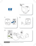
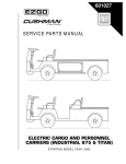
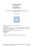
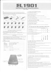
OctoNus Software Ltd
Helium Polish - system for scanning of diamonds
User manual
Please read carefully this manual before starting to work with Helium system.
Contents
page
1. FUNCTIONS AND POSSIBILITIES....................................................................................... 3
2. COPYRIGHT. ........................................................................................................................ 4
3. SAFETY REGULATIONS...................................................................................................... 4
4. HELIUM SYSTEM SET. ........................................................................................................ 5
5. DESCRIPTION OF FUNCTIONAL PARTS OF HELIUM SYSTEM....................................... 6
6. HELIUM SYSTEM CONNECTION. ....................................................................................... 7
6.1. Computer requirements.................................................................................................................................................7
6.2. Connection to computer and software installation. ...............................................................................................7
7. START AND FIRST STEPS. ................................................................................................. 8
7.1. Switching on and system verification........................................................................................................................8
7.2. Scanning and building of model. ..............................................................................................................................11
7.3. Working with model, possibility of using. ..............................................................................................................14
7.4. Reports and their contents. ........................................................................................................................................17
7.4.1. Description and calculation of the report parameters. ...........................................................................27
7.5. Verification of system settings with help of gauges............................................................................................37
7.6. Helium system tuning. (Temporarily option is unavaible!). ...............................................................................39
8. ENRICHED FUNCTIONALITY OF HELIUM SYSTEM (UNDER CONSTRUCTION!). ........ 40
9. TROUBLESHOOTING. ....................................................................................................... 41
10. SPECIFICATION. .............................................................................................................. 42
2
1. Functions and possibilities
Helium scanner is new device for cutting factories, gemological laboratories and distributors. Scanner is
assigned for scanning of diamonds and semipolished diamonds, and for creation of its 3d-models by angles of
inclines and azimuths of facets.
Possibilities:
1. This time scanner allows to create perfect models with high accuracy of round diamonds and fancy cuts
“Oval”, “Pear”, “Marquise”.
2. Exact building and visualization of model allow to determine big and small deviations of symmetry.
3. Possibility to estimate diamond proportions by different Cut Grading Systems.
4. Helium scanner allows to measure azimuths of facets inline of the diamond. Existent scanners measure
angles of facets incline using “silhouette” method. But each facet has not only angle of incline; it has its
own azimuth of incline which is shown on the model built by Helium scanner.
5. Helium software creates Reports with structure and content defined by user. Reports include various
information about diamond parameters. In particular, it is possible to create full detailed Report of scanned
stone (see item 7.4).
6. Helium scanner identifies naturals and extra facets on the diamond and creates the model with additional
facets in the case if these additional facets exist on the diamond.
7. Helium system allows to create accurate 3D-models of semipolished diamonds and control angles and
sizes of diamonds on intermediate stages of cutting manufactures.
8. Software has option which allows to model recutting of diamonds for the improvement of proportions and
symmetry.
Helium scanner is the most accurate scanner for scanning and building of 3d-models, which is necessary
for modern diamonds manufacturers and laboratories making appraisal of cut quality.
Fig. 1. The photo of Helium system. At the foreground there is scanner, on the left – computer, at
the background – monitor with interface image of Helium software.
3
2. Copyright
Technology of Helium scanner is protected by copyright and intellectual property laws. All rights of
manufacturing of this device are owned to OctoNus Ltd. This device is assigned for using at cutting factories,
gemological laboratories and for other similar purposes, if it is not prohibited by OctoNus Ltd. Unapproved
technical changes, disassemble of the device and change of software are prohibited.
3. Safety regulations
Carefully study these regulations before starting of scanner using.
1. Don’t locate the device to places with critical temperatures (more than 400С and less than -200С). Avoid
temperature excursions: if the scanner was fast transported from the cold place to the warm one, drops of
moisture can appear on its surface or inside. In this case keep it at the room temperature for minimum 1
hour before switching on.
2. Avoid moisture and dust. Don’t use the scanner in dust-laden places, in places with high moisture, avoid
water falling. It can lead to the malfunction of the device.
3. It is prohibited to subject the scanner to careless handling, shaking and sharp blows during transportation.
Otherwise it will lead to irregularity of alignment of components inside the device. Don’t turn the scanner
upside-down. Place the device to horizontal position, don’t put heavy objects on the scanner.
4. Use smooth dry fabric or cotton-wool spirit tampon to wipe outside components of the scanner and rotating
support-holder. Use special tools for caring and cleaning for optical parts of the device. Don’t use liquid
chemical cleaners and compressed air to remove the dust.
5. Don’t use force to any part of the scanner. Don’t disassemble and don’t try to repair it independently.
6. If any outside objects are felt into scanner, stop scanner using and contact to Support Service.
7. Don’t touch internal parts of the scanner by hands or by other objects.
8. At the first switching on of system and also at cases of “switching off – switching on” of system after
switching on it is necessary to wait about 1-2 hours before start of work to get correct results of camera
work.
9. It is recommend to don’t switch off Helium system absolutely and connect it to the power by the
uninterrupted power supply.
4
4. Helium system set
№
1
2
3
4
5
6
7
8
9
10
Name
Main block
Frame grabber Matrox Meteor-II /Standard
Video-cable (coaxial)
Power cord
Software CD
HASP key
Vacuum pump Nitto VP0125
USB-cable A-B
Silicon tube
User manual
Quantity
1
1
1
2
1
1
1
1
1
1
Fig. 2. Helium system set.
5
5. Description of functional parts of Helium system
Fig. 3. Description of functional parts of Helium system.
1.
2.
3.
4.
5.
6.
7.
8.
9.
10.
11.
12.
13.
14.
15.
16.
17.
18.
19.
Object for scanning
Camera aperture
Laser aperture (Attention! – laser is not provide for this model of system)
Label with the name of manufacturer and scanner serial number
Video out (to connect with framegrabber)
Vacuum connector (to connect with pump)
Service connector (is not using for this model)
USB-connector (to connect with computer)
Cover (to isolate superfluous light during scanning)
Support-holder with aperture for air extraction
Main block of Helium system
Vents (hold them opened)
Socket (220V/110V, to connect power supply to pump)
Switch of the scanner
Socket (220V/110V, to connect power cable to scanner)
Vacuum pump
Pump switch
Socket (220V/110V, to connect power supply from main block)
Silicon tube (connection between pump and scanner).
6
6. Helium system connection
6.1. Computer requirements
- Pentium 4
- HDD 60 Gb
- RAM 256 Mb
- 1 small PCI port for Matrox framegrabber (see compatibility list of motherboards here
ftp://ftp.matrox.com/pub/imaging/pccompat/Meteor2.pdf. In the case if you can’t find newer motherboard model,
contact with Matrox)
- 2 USB ports for HASP key and system control
- Windows 98/2000/XP
- Microsoft Word for printing reports.
6.2. Connection to computer and software installation.
Attention! In the case of sudden change of temperature/humidity conditions (for example, transportation of system
from cold to well-warming room) moisture is accumulated on optic parts of scanner. Therefore don’t switch on
scanner during 1-2 hours after transportation. Wait for a 1-2 hours after every switching on of system. It is
necessary for correct results of camera work and stability of Helium system work.
1. Pull out the scanner and component parts from packing.
2. Insert the frame grabber “2” (see Fig. 2, here and hereinafter in this chapter) into the PCI slot of computer
motherboard
Attention! – it is necessary to shut down computer before operation to avoid electrical shock hazard.
Switch on computer and log on to computer as “Administrator” (permissions of administrator are necessary
to install programs and drivers). After loading, the operating system automatically will offer you the
installation of driver for the frame grabber. In this case it is necessary to press Cancel and launch program
CD-ROM drive (D:):\Matrox\Setup.bat from Compact Disk “5” and follow instructions of wizard:
- After query of wizard “Select the board driver(s) that you want to install, Meteor-II /Digital or Meteor-II
/Standard” choose Meteor-II /Standard.
- Follow wizard and don’t change default directions.
- Restart computer after wizard finished work.
3. Insert HASP-key “6” into USB port and launch program CD-ROM drive (D:):\hdd32.exe from CD. Follow
instructions of wizard and install driver of HASP-key. In the case of successful installation a red lamp on
the key is turned on.
4. Connect the power cable “4(1)” to the main block of scanner “1”.
5. Connect main block “1” and vacuum pump “7” with help of power cable “4(2)” using transformer.
6. Connect the frame grabber “2” and main block of scanner “1” with help of the coaxial video-cable “3”.
7. Connect vacuum pump “7” and main block “1” with help of silicon tube “9”.
8. Connect computer and main block “1” with help of USB-cable A-B “8”.
9. Switch on the scanner (the switch is on the main block “1”) and vacuum pump “7”.
10. After switching on, the operating system will find new hardware and launch wizard. Choose manual search
of driver and indicate the path to CD-ROM drive (D:):\HeliumBoard\. Click OK. In the case of appearing
of inscription on the screen about absent of digital signature: “The software you are installing for this
hardware: … has not passed Windows Logo testing to verify its compatibility with this version of Windows
and etc.” click “Continue anyway”.
11. To install HeliumPolish software, launch CD-ROM drive (D:):\setup.exe and follow instructions of wizard.
7
7. Start and first steps. Main Helium functions
7.1. Switching on and system verification
1. Open Device Manager of your computer - by right button of the mouse click on My computer, choose
Properties from menu, in opened panel choose bookmark Hardware and press on the Device manager.
2. Make sure that all installed devices work properly:
2.1. Matrox Imaging Adapter/Meteor_II PCI Frame Grabber
2.2. Universal Serial Bus Controllers/Aladdin USB Key
2.3. Universal Serial Bus Controllers/OctoNus Helium Device.
Devices work properly if on the icons corresponding to them, during Device manager starting there are no
“red cross” or “yellow question-mark”.
If there are any problems with new installed devices (it is disconnect – “red cross”, or there are no driver “yellow question-mark”, or it is not installed and there are no such device in the list), try to repeat all steps
described in previous chapter thoroughly. If faults were not corrected, apply to Service Centre.
3. Switch on main block of scanner, pump and start file Helium.exe from the Folder you installed software (by
default it is C:\Program Files\OctoNus Software\Helium), or with help of commands “Start-ProgramsHelium-OctoNus Helium 3.5”.
Fig. 4. Image of software screen.
1 – free region of software (background)
2 – Display panel
3 – Scan polished diamond panel
4 – Main menu of Scan polished diamond panel
5 – Scene
8
Fig. 5.
1 - main menu of the program
2 - image of scene after pressing Camera button
4. Press by right button of the mouse on free region of software (free region is background as blue ornament,
see 1 at Fig. 4), choose Restore, and then choose Display (see Fig. 4). At the window Display (see 2 at
Fig. 4) next inscriptions will appear: “Photo device was loaded successfully”, “Engine device loading
successfully”. If there are another inscriptions, then:
4.1. Exit program: point mouse to upper part of window, and press Exit button in pop-up window (see 1 at
Fig. 5)
4.2. Check connection of scanner to computer and framegrabber (by USB and coaxial cables)
4.3. Start software again. If faults are still presenting, contact to Service Centre.
If necessary inscriptions are presenting, fold the window Display. To make it, press the button with image
of “tick” at the upper right corner of the screen (To unfold this window, click on free region by the right
button of the mouse, choose Restore, choose Display illuminated with green color!).
! You can move and change the dimension of panels the same way as in Windows operating system. To
move panel, drag it by upper part with pressed left button of the mouse. To change its dimension, point the
will appear. Change dimensions of the panel holding pressed left
mouse on the corner, the icon
button of the mouse.
5. Checking camera availability.
After starting the program, Scan polished diamond panel (see 3 at Fig. 4) will appear. At the panel Build in
main menu of Scan polished diamond panel on the right part of the window (see 4 at Fig. 4), press the
button Camera (
) or press F12 on the keyboard. The icon will become as colored (
). Then
check is there image on the scene (see 5 at Fig. 4), which there exists at Fig. 5 (2). Positive result means
that camera and framegrabber work properly.
6. Checking of motor availability.
Open the cover of the scanner (see 9 at Fig. 3). At Build panel of main menu of Scan polished diamond
panel (see 4 at Fig. 4), press buttons Right (
) and Left (
) for several times. Make sure that
9
support-holder is rotating during pressing of these buttons. If motor is not working, open Motor panel,
choose Other bookmark and press the button Go near inscription InitRx (to initialize axe of rotation Rx).
Initializing of motors will happen – the support-holder is rotating. If motor is not rotating after you pressed
Go button, check connection of scanner to computer and switching on of the scanner. If anyone of above
procedure is not successful, contact to Service Centre.
7. Checking of vacuum pump availability.
Open Motor panel, choose Motor bookmark and press Pump button
(or press Ctrl+F9 on the
keyboard). You should hear the sound of working pump. Check if the air is drawing from support-holder. If
the air is not drawing from support-holder, check switching on of the pump, correctness of connection of
silicon tube. If it doesn’t help, contact to Service Centre.
8. After you made above tests, you can start to work.
10
7.2. Scanning and building of the model
The first stage of working with scanner is scanning and building of the model. Use gauge (sample round
stone which is applied to delivery set) as first object for scanning. It is necessary by two reasons:
- It is easier to study scanning, to build the model and to get first results on the object, which is passed tests
already.
- Gauge will be used in future to align Helium system. It is necessary stage before starting to work. With help of this
gauge you can check the level of alignment of Helium system, to control the possible fault or changes of alignment
after transportation.
The starting of the work
1. Switch on the scanner, enter the program and check system availability (see previous chapter).
2. Open Motor panel, choose Motor bookmark and press Pump button (
), or only press Ctrl+F9 on the
keyboard. When pump will switch on and work, go to the next item.
3. Take object for scanning.
4. Thoroughly wipe object for scanning by dry cotton rag (it is better to use special rag for diamond cleaning).
5. Open cover “9” (Fig. 3) of main block “11” (Fig. 3) of the scanner.
6. Take object with tweezers by girdle and put it to the center of support-holder.
7. Check the location of object on the support-holder. To do it, slightly press Camera button
or key F12
on the keyboard. Now you see image of object on the scene of the program. It is necessary borders of
object will not exceed of scene frame (see 1 at Fig. 6). Using buttons for motor rotating in Build panel of
main menu of Scan polished diamond panel (Right
and Left
), turn the support-holder with
object on 180 degrees and make sure that image is not exceed of scene frame in every position (you can
change motor step using button
panel.
(see 2 at Fig. 6), which is near Step for motor inscription at Build
NOTE! The buttons like this
which are presented in the program in different panels have following principle of
operation:
1. Field with text or digital value is situated near the button. You can change value of field by pressing mouse
button on upper or lower part of button
.
2. Single pressing of right mouse button on the upper part
increases value fast, on the lower part
decreases value fast,
text values are changed by pressing.
3. Pressing and holding of right mouse button changes value with high velocity up to limit.
4. Single pressing of left mouse button changes value on one step..
5. Pressing and holding of left mouse button changes value progressively with increasing velocity up to limit.
11
Fig. 6. Image of screen after placing of object for scanning.
1 – image of correct placing of object on support-holder on the scene
2 – button to change the step of motor
3 – Start button
8. After you correctly place object for scanning, it is necessary to make sure of its clearance. Check the
absence of visible dust using buttons to control the motor and the image on the scene (the best way is: to
set the step of motor equals 22.5 degrees and to rotate the object on 180 degrees, every time checking
object clearance with help of image). If there is some dust on the object, take it with tweezers, wipe it again
and set on support-holder. Check the absence of dust. Also it is possible to wipe object not taking it away
the support-holder. To do it, take cotton-wool tampon and spirit, wet tampon and carefully wipe accessible
parts of the object (Don’t press the object!).
9. Close scanner cover. Make sure one more time of the object clearance using buttons for motor rotation.
Also check the clearance of visible part of support-holder. If there is dust on it, remove this dust using
tampon wet with spirit.
10. Press Start button (see 3 at Fig. 6) at Build panel of main menu of Scan polished diamond panel and wait
for about 1 minute while object is scanning and model is building (you will see image of “hour-glass” near
cursor during work of program – don’t make any actions till the image of “hour-glass” disappear). After
finishing of scanning and building of the model, image of model, matching with object photo, will appear on
the scene of the program (see 1 at Fig. 7); Model (see 2 at Fig. 7) and Parameters (see 3 at Fig. 7) panels
will be opened in main menu of Scan polished diamond panel; name of scanned object as Simple and
information about its model (diagram of diameter values, girdle shape, angles of pavilion and crown for
each facet, will appear under the scene – see 5 at Fig. 7).
11. The clearance of the object is very important for correct building of the model, so there is automatic
checking of object clearance. This procedure is realized by analysis of inscriptions at Model panel after
model is built. At the first stage it is necessary to check inscription at upper line of Model panel. Inscriptions
of green color such as Model was built correctly or Model has noncritical errors mean that model was built
satisfactorily for further work. Inscriptions of red color such as Model was built very bad or Model was not
built mean that it is necessary to rebuild the model. Try to clear the object one more time and scan it again
by pressing Start and OK buttons.
(Attention! Model can be built incorrectly by another reasons not depended on object clearance. If you can’t
build model correctly by object clearance, follow instructions of chapter “Troubleshooting” or contact to Service
Centre).
12
Fig. 7. Image of the screen after scanning and building of model of object.
1 – model of object matching with photo at the scene
2 – Model panel
3 – Parameters panel
4 – Panel of objects
5 – Panel with information about scanned object
6 – Scene menu of Scan polished diamond panel
7 – Compare scans button
12. If you see green inscription, we congratulate you with correct building of the model. After it we recommend
you to save project.
Note! Saving of the project. In main menu of the program with help of mouse press “Start” button and choose
point “Save project as…”. The window “Save project data” will be opened. Similar way you work with Windows
operating system, choose folder where you want to save the project (by default it is folder where Helium software
was installed – C:\Program Files\OctoNus Software\Helium) and name the file at field “File name”. Then press
“Save” button.
Note! Opening of the project. To open saved project, press “Start” button of main menu of the program and
choose point “Open project…”. Choose the file you want to open.
Note! Exit of the program. To exit from the program, save project and press “Exit” button. If you didn’t save
project, but changed it, program asks you to save changes in the project or exit without save.
13
7.3. Working with model, possibilities of its using
Edge model built by software with help of scanning, has its own parametrical characteristics. Partially these
characteristics are shown in Parameters panel of main menu of Scan polished diamond panel (see 3 at Fig. 7) and
in panel of object information (see 5 at Fig. 7). Here we say “partially” because full information includes very big
content and is contained in separate report, generated by program (you can read about it below).
Panel of object information
1. In first line there is information about stone diameter and diagram of its values distribution on circle of
scanned stone. Red color is for minimum value, green color is for maximum value, gray color is for
medium value.
2. Further there is girdle figure by circle of the stone.
3. Further there is information about pavilion angle. You see values of incline angle of each facet of pavilion.
Colors are distributed similarly colors for diameter (see point 1).
4. In last line there is information about crown angles. You see values of incline angles for each facet of
crown. Colors are distributed similarly colors for diameter (see point 1).
In panel all data of every line are coordinated each other, e.g. indication of values and girdle image start
from the same initial point and further along the circle. There are small sections between values of angles of
pavilion and crown, which are passed from values. These sections mean coordination of facets of pavilion and
crown (or rather speaking, this is difference between values of azimuths for facets). Because pavilion facet and
corresponding crown facet can have different azimuths (they can be slightly turned relatively each other), then
sections passing from values of pavilion and crown, may not converge together.
“Parameters” panel
In this panel there is the following information (top-down):
1. In first line there is weight (Weight, ct) of scanned stone (based on dimensions of the model) – first value is
rounded to two digits, second value is rounded to four digits. Is it customary in Cut Grading System, roundoff to two digits is made in the following way: if the weight of the stone A.BCDE less than A.BC85, then we
write A.BC; if it is greater than A.BC85, then we write A.B(C+1).
2. Next line is value of total height (Total height, mm) of the stone, rounded to third digit and the value in
percents from medium value of diameter, rounded to first digit.
3. Values of diameter (Diameter, mm) are Avg (average), Min (minimum) and Max (maximum)
correspondingly.
4. Values of pavilion angle – Pavilion angle, 0.
5. Values of pavilion depth in percents from medium diameter – Pavilion depth, %.
6. Values of crown angles – Crown angle, 0.
7. Values of crown height in percents from medium diameter – Crown height, %.
8. Values of table diameter in percents from medium diameter - Table, %.
9. Values of girdle thickness in percents from medium diameter (Girdle thickness, %). These measurements
are made at wide place of girdle (Bezel), medium place (Bone) and narrow place (Narrow).
10. Value of culet in percents from medium diameter (Culet, %).
11. Further there is section named OctoNus measurements (measurements of OctoNus Ltd.) with values of
pavilion (Pavilion angle, 0), and crown (Crown angle, 0) angles, measured by different way than values in
above points. You can read about these measurements in details in chapter “Reports and its contents”.
12. In last line there is total difference between azimuth values of facets of crown and pavilion (Twist, 0).
You can read about calculation of data values and other parameters in chapter “Reports and its contents”.
There is field Weight at the bottom of Scan polished diamond panel where user can set weight of the stone
manually (measured it on the scale).
After scanning in scene window of Scan polished diamond panel, user can work with the model, using mouse and
panel of object under the scene (see 4 at Fig. 7).
Control of mouse in scene window
Point cursor of the mouse at the scene window. Pressing and holding left button of the mouse, move cursor along
the scene. Model is moving or rotating. Rotating or moving of the model is determined by pressing of keyboard
keys combination:
Note! System axes disposition is: X axis is directed from us (into scene), Y axis is directed to the left (horizontal
axis), Z axis is vertical axis.
14
Shift+1 - moving of cursor to the left-right is moving of object along Y axis, moving of cursor to up-down is moving
of object along Z axis;
Shift+2 - moving of cursor to the left-right is moving of object along Y axis, moving of cursor to up-down is moving
of object along X axis;
Shift+3 - moving of cursor to the left-right is moving of object along X axis, moving of cursor to up-down is moving
of object along Z axis;
Shift+4 - moving of cursor to the left-right is rotating of object around Z axis, moving of cursor to up-down is
rotating of object around Y axis;
Shift+5 - moving of cursor to the left-right is rotating of object around Z axis, moving of cursor to up-down is
rotating of object around X axis;
Shift+6 - moving of cursor to the left-right is rotating of object around X axis, moving of cursor to up-down is
rotating of object around Y axis;
Shift+7 - moving of cursor to the left-right and up-down is increasing-decreasing of object dimensions;
Shift+8 - moving of cursor to the left-right is increasing-decreasing of object dimensions; moving of cursor up-down
is moving of object along Z axis;
Shift+9 - moving of cursor to the left-right is decreasing of sensitivity of mouse moving;
Shift+0 - moving of cursor to the left-right is increasing of sensitivity of mouse moving.
Besides mouse control, you can control moving of objects with help of Movement panel (see Fig. 8), which is
opened by pressing button
in main menu of the program. In this panel in field Angle you can set step for
rotation angle of object and near there are buttons which rotate object. In field Factor you can set coefficient of
dimension change.
is decreasing of dimension,
is increasing of dimension. In field Dist you can set
the step for object moving, and near there are buttons to move object in some direction.
is moving to us,
is moving from us.
Fig. 8. Panel of moving of object.
If you point mouse cursor on certain facet during the work with model in scene window, then near mouse
pointer will appear “cross” image; and in upper part of scene window will appear inscription like as: Simple: Side
(21), @ 102.130:41.650, which includes information about incline angle and facet azimuth. Simple is model name,
Side (21) is its facet and number, @ 102.130 is facet azimuth, 41.650 is incline angle of facet.
15
Panel of objects
Panel of object is located under the scene and you can its image below
Fig. 9. Panel of objects. From the left to the right: field with object name, button of
object visualization in the scene, button of model activity, button for deleting the object
from scene, button to call panel with object properties, button of visualization of
inclusions (last button is workable after creating of object inclusions).
In this panel you can change the name of object. Press by left button of the mouse on field with the name
of object and print new name. There are five buttons at the right from the name of object. Usually for work first four
buttons are used. The last one is necessary to work with inclusions in rough diamonds. Below you see description
of the action when you press left (not right!) button of the mouse on each button of the panel of objects.
First button allows to enable and to hide visualization of object at the scene (note that if the object remains
in the scene when the button is turned off, then user can’t see it).
Next button is for turning on-turning off of object activity. If the button is turned on, then during changing,
moving or rotating of object by the mouse or by panel of object (see further), position of object is changed at scene
basis. At the same time the link of object with photo is lost and after you turn off the button, its new position is
saving relatively to basis, photo and motor position. At turned off button when you move mouse, you change
positions of scene basis. Object position is fixed relatively to basis and the link with photo and motors position is
saved.
Third button deletes object from the scene (it is important that object is not deleted from the project, it is
deleted only from the scene). All objects of the project are saved in Figures panel, which you can open by left
button of the mouse in main menu of the program. To place object, which exists in project, to the scene again, it is
necessary to mark this object in Figures panel by the mouse. The name of object will appear in the button at the
bottom of panel (
). Press this button with the name of object and holding it move object on
the scene, release mouse button. Object will appear in the scene again.
Forth button opens panel of object properties.
Fifth button is for visualization of inclusions.
Above you saw short information panel of objects. More detailed information see in chapter “Enriched
functionality of Helium system”.
Next step to work with model is opening of Report from MS Word and its printing.
16
7.4. Reports and its contents
The section concerning Reports is located in the menu of scene of Scan polished diamond panel (see 6 at
Fig. 7) in Report submenu. Press Report by the mouse, following available options will be accessible (see fig. 10):
•
•
•
•
•
•
•
“Set default menu for cutting” – you can choose default action which will be realized after you push button
“Report” (near button “Scan” in right block of panel “Scan polished diamond”) – you can choose operation
of printing or opening of any type of report. Last button is for printing of labels (Label Printer device is
necessary).
“Automatically print report” – if you mark this action then immediately after scanning and building of model
program automatically will execute default operation (see above) without intermediate operations.
“Print Report” and next menu “Open Report”. You can print and open in MS Word any type of report. If you
work with semipolished diamond then choose action “Full color report for semi-polished brilliant” or “Full
B&W report for semi-polished brilliant”. If you work with rounded fancy cuts (Marquise, Oval or Pear) then
choose “…report for rounded fancies”. If you work with rectangular cuts then choose “…for rectangular
fancies”. Please don’t forget to choose necessary cutting in Build bookmark of main menu of panel “Scan
polished diamond” before scanning.
“Export report Data” is necessary for export data in application which was choosed by user.
“Export report Data for compare” is option for test of Helium system alignment and checking of
repeatability of results. See detailed information in chapter 7.5. Checking of alignment of the system with
help of gauge is point 3 of chapter 7.5.
“Print Label”. You can print label if you have installed device “Dymo Label Printer” on your computer.
“Export model…”. After you press this button program open panel “Write side information for Simple”
where you can export model to one of 3 formats (see fig. 11). Please enter file name (Model1 by default)
and press right button of mouse on the free field near inscription “Save as type” (“OctoNus scanner file
(*.osf)” by default) and choose necessary format: “OctoNus scanner file (*.osf)” or “Pacor export data
format (*.mmd)” or “Diamond calculator diamond format (*.dmc)”. If you choose *.dmc you can open saved
model in program DiamCalc 2.3.1 or later version. Press “Save”.
Fig. 10. Report submenu.
17
Fig. 11. Panel “Write side information for Simple”.
Helium Standard Report for polished diamond.
HELIUM STANDARD REPORT
Polished Brilliant
4.776 mm (4.763 - 4.792)
100.0%
General information
Model
Expert name
Report date
Real weight, ct
Calculated weight, ct
Total height
Total height quality
Appraiser title
Overall cut quality
Overall symmetry
quality
63.8%
KB-7
Savrasov S.
08.12.2004
0.3760
0.37, 0.3763
2.722 mm, 56.99 %
N/A
GIA
G
PR
11.4%
32.23°
Star
Ratio
58.8%
2.9%
40.65°
42.7%
57.0%
2.722 mm
Length
Girdle
Facet
83.5%
Depth
Girdle
Facet
84.8%
0.6%
Main parameters
Parameter
Diameter
Crown angle
Crown height
Pavilion angle
Pavilion height
Pavilion halves angle
Upper facets angle
Star facets angle
Star :
Upper ratio
Table
Culet
Twist
Girdle thickness: Bezel
Girdle thickness: Bone
Girdle thickness: Valley
Average value, mm
mm
°
%
°
%
°
°
°
%
%
%
°
%
%
%
C-Height
0.545
Avg
4.776
32.23
11.41
40.65
42.67
41.55
39.87
18.78
58.83 :
41.17
63.76
0.56
1.39
2.86
3.33
1.56
P-Height
2.038
Min
4.763
31.06
10.66
39.67
41.68
40.59
38.94
17.46
54.56 :
45.44
63.62
0.38
0.03
2.38
2.99
1.23
Table
3.046
Max
4.792
32.56
12.40
41.48
43.73
42.46
40.98
19.82
63.44:
36.56
63.83
0.67
3.68
3.43
3.76
2.02
Culet
0.027
Dev
0.61 %
1.51
1.75
1.80
2.04
1.87
2.04
2.36
Cut
E-VG
G
N/A
N/A
G
-
Sym
EX
VG
VG
VG
GD
VG
GD
GD
8.88
-
PR
0.20
0.29
3.65
1.05
0.77
0.79
G
N/A
N/A
EX
EX
VG
EX
EX
EX
G-Bezel
0.136
N/A
G-Bone
0.159
G-Value
0.075
18
There is the following information in this report (by lines):
- Name of the model;
- Name of expert which you can set in the program in main menu of Scan polished diamond panel in Info
bookmark in Expert field. Here you can also change date if it is incorrect;
- Date of Report;
- Real weight of the stone if it is entered to the program (see chapter “Working with model, possibilities of its
using”, the section concerning work with Parameters panel);
- Weight of stone model;
- Total height of stone model in mm and in %;
- Estimation of total height quality by appraiser;
- Name of appraiser. You can choose necessary appraiser in the program in main menu of Scan polished
diamond panel in Bookmark Recutting in field Grading;
- Total cut quality of whole stone model by choosed appraiser;
- Total symmetry quality;
- Table with indications of parameters; its measure units; average, minimum and maximum values;
difference in percents between maximum and minimum values. Further there is appraising of parameter by
preliminary chosen Cut Grading System, and appraising of symmetry of parameter (by difference between
maximum and minimum values).
- Table with parameters values in mm.
Detailed description of parameters and the way of its measuring see at the end of this chapter.
1.1. Illustrated B&W report. This report is for internal using in gemological laboratories. It can be delivered to
user is necessary be cause it has more detailed structure and has more information.
Here there are values of parameters for each facet of the model, pictures of the model with signed
parameters values, there are diagrams of girdle shape, distribution of diameters values, distribution of
radius values. This information is necessary for detailed studying of the stone.
1.2. Illustrated color report. This report is similar to previous one but with colored pictures.
1.3. Full B&W report. This is most detailed and informative type of report is for cutting factories, to trace the
shape of cut and for recutting of stones. Here there are tables with most full set of different parameters,
and further there are pictures of the model from different directions with indication of data necessary at this
factory.
1.4. Full color report. This report is similar to previous report with colored pictures.
1.5. 8-Facet report for round brilliant. This is report which contains information about all facets of brilliant.
If you use any report and you have questions concerning its information, please contact Service Centre.
19
HELIUM ILLUSTRATED REPORT
Polished Brilliant
KB-7
Savrasov S.
08.12.2004
0.3760
0.37, 0.3763
0.03 ct, 8.34%
4.776 (4.763-4.792) x 2.722 /0.017
0.136
0.159
0.075
4.776 mm (4.763 - 4.792)
100.0%
63.8%
11.4%
32.23°
Star
Ratio
58.8%
2.9%
40.65°
42.7%
57.0%
2.722 mm
Length
Girdle
Facet
83.5%
Depth
Girdle
Facet
84.8%
0.6%
55.0°
90°
0°
0°
180°
202.0° 4.792mm (max)
270°
12.40
43.73
63.83
1.75
2.04
0.20
EX
VG
VG
VG
GD
EX
Upper girdle angle, ° 39.87
38.94
40.98
2.04
-
GD
Star angle, °
Lower girdle angle /
Halves angle, °
Star:
Upper ratio, %
Culet, %
Twist, °
18.78
17.46
19.82
2.36
-
GD
41.55
40.59
42.46
1.87
-
VG
58.83:
41.17
0.56
1.39
54.56:
45.44
0.38
0.03
63.44:
36.56
0.67
3.68
8.88
-
-
0.29
3.65
N/A
-
Girdle Bezel, %
2.86
2.38
3.43
1.05
Girdle Bone, %
3.33
2.99
3.76
0.77
Girdle Valley, %
1.56
Total height, mm
Crown height, mm
Pavilion depth, mm
Table, mm
Culet, mm
Girdle Bezel, mm
Girdle Bone, mm
2.722
0.545
2.038
3.046
0.027
0.136
0.159
1.23
2.02
0.509
1.991
3.039
0.018
0.114
0.143
Girdle Valley, mm
0.075
EX
VG
0.10
0.57
0.71
N/A
EX
2.91
2.38
3.43
-
EX
3.07
3.59
3.41
3.12
3.76
2.99
3.58
3.11
1.46
1.63
1.24
1.38
1.42
1.27
2.02
1.23
1.98
1.43
1.76
1.70
1.67
1.79
1.40
1.60
0.592
1.991
3.047
0.583
2.019
3.049
0.554
2.006
3.048
0.518
2.051
3.039
0.509
2.079
0.509
2.089
0.537
2.057
0.560
2.015
0.139
0.147
0.070
0.078
0.114
0.171
0.059
0.066
0.164
0.163
0.068
0.061
0.152
0.149
0.096
0.059
0.131
0.180
0.095
0.068
0.120
0.143
0.084
0.081
0.124
0.171
0.080
0.085
0.147
0.149
0.067
0.076
-
-
24.93
270°
235.0° 4.763mm (min)
Azimuths deviation from ideal
1
2
3
4
Pavilion, °
Lower girdle facets / Pavilion
Halves, °
Crown, °
0.00
-0.26
1.17
-0.10
-1.45
-3.77
-1.36
0.10
2.08
1.46
0.66
2.14
5.28
-1.90
0.18
-1.39
1.14
-0.53
-1.37
0.39
-0.40
1.35
0.73
0.58
-0.56
0.13
2.94
-2.09
Upper girdle facets, °
Star facets, °
40.65°
32.46°
40.31°
40.59°
41.03°
GIA
10.66
43.53
10.66
43.73
11.24
43.07
11.73
42.19
40.16
40.98
17.46
40.65
42.24
63.44:
36.56
39.56
39.52
18.27
41.03
42.04
60.82:
39.18
39.22
39.37
18.06
41.38
41.77
58.13:
41.87
39.84
39.79
19.82
41.56
41.34
54.56:
45.44
1.91
3.68
0.94
0.03
3.20
3.18
2.75
2.52
2.59
3.08
Girdle to MIC, mm
0.017
6
1.32
0.93
0.13
-2.36
-1.56
-0.33
0.04
7
0.20
1.70
0.27
1.14
0.57
5.03
1.28
8
-0.01
1.73
-0.23
0.02
-1.38
1.48
0.81
-0.15
1.56
-0.22
3.04
0.51
0.33
1.35
39.56°
31.06°
39.55°
18.55°
19.32°
41.09°
41.56°
-888.88°
40.34°
19.82°
17.46°
39.37°
40.86°
38.94°
42.04°
42.41°
42.46°
18.06°
42.24°
41.04°
41.39°
32.56°
Girdle center
0.125
0.119 MIC
0.000
Pavilion
0.0° 22.5° 45.0° 67.5° 90.0° 112.5° 135.0° 157.5° 180.0° 202.5° 225.0° 247.5° 270.0° 292.5° 315.0° 337.5° 360.0°
Diameter, mm
4.792 max
4.776 avg
4.763 min
4.746 MIC
0.000
-0.025
22.0°
55.0°
202.0°
235.0°
0.0° 22.5° 45.0° 67.5° 90.0° 112.5° 135.0° 157.5° 180.0° 202.5° 225.0° 247.5° 270.0° 292.5° 315.0° 337.5° 360.0°
39.52°
Radius deviation, mm
0.100
Radius, mm
0.075
0.050
2.406 max
0.025
18.27°
40.98°
40.98°
-888.88°
41.48°
40.10°
32.25°
2.373 MIC
0.000
0.0° 22.5° 45.0° 67.5° 90.0° 112.5° 135.0° 157.5° 180.0° 202.5° 225.0° 247.5° 270.0° 292.5° 315.0° 337.5° 360.0°
-888.88°
32.54°
Culet center
0.358
0.239
2.50
0.00
Girdle thickness, mm
0.478
-888.88°
32.41°
41.77°
42.23°
5.00
0.025
39.84°
32.41°
-888.88°
41.34°
41.83°
Crown
0.050
39.22°
41.10°
-888.88°
40.75°
7.50
0.075
19.24°
19.50°
Girdle thickness, %
10.00
Diameter deviation, mm
0.100
40.16°
39.60°
41.08°
39.79°
Symmetry
Polish
Color
Clarity
Fluorescence
32.56
41.04
E-VG
39.27°
G
PR
32.54
41.48
G
-
32.10°
-888.88°
41.38°
Overall symmetry quality
32.25
41.39
31.81
40.61
Yes (2)
5
39.67°
-888.88°
40.17°
Overall cut quality
32.41
40.75
32.41
32.35 32.32
40.55
40.85 40.57
Extra Facet / Nat
-
40.22°
Appraiser title
8
10.83
42.93
63.62
40.22
40.10
18.55
40.59
42.46
59.24:
40.76
-
Culet through Crown Bezel, °
7
11.59
42.00
63.81
39.60
40.98
19.24
41.08
42.41
60.87:
39.13
0.083
0.098
0.010
0.014
0.050
0.037
0.30
0.60
6
12.21
42.26
63.83
39.27
38.94
19.50
41.10
42.23
58.50:
41.50
0.592
2.089
3.049
0.032
0.164
0.180
40.85
32.41
3.64
5
12.40
41.68
63.79
39.55
40.86
19.32
41.09
41.83
55.04:
44.96
EX
0.038
4
4.776
31.06
40.17
N/A
0.096
3
4.775
32.10
39.67
N/A
-
0.059
2
4.772
32.46
40.31
0.79
Measurement as per OctoNus theory:
Crown angle, °
40.65
40.55
Pavilion angle, °
32.23
31.81
Fish eye effect, °
1
4.783
32.41
40.34
90°
22.0°
180°
10.66
41.68
63.62
E-VG
G
N/A
N/A
N/A
G
G
val=1.2%
0.027
0.61%
1.51
1.80
bone=3.0%
3.046
Valley
4.792
32.56
41.48
bone=3.8%
2.038
Bezel
4.763
31.06
39.67
bzl=3.4%
0.545
Culet
Girdle
Bone
Sym
4.776
32.23
40.65
56.99
11.41
42.67
63.76
val=2.0%
Average values, mm
Crown
Pavilion Table
height
depth
Avg Min Max Dev Cut
Diameter, mm
Crown angle, °
Pavilion angle, °
Total height, %
Crown height, %
Pavilion depth, %
Table, %
bzl=2.4%
Model
Expert name
Report date
Real weight, ct
Calculated weight, ct
Spread
Measurements, mm
Parameter
Тable center
Girdle-Culet offset
Girdle-Table Offset
Table-Culet Offset
(by table axis)
(by table axis)
(by table axis)
1.46 ± 0.26, %
0.070 ± 0.012, mm
1.21 ± 0.23, %
0.058 ± 0.011, mm
1.83 ± 0.27, %
0.087 ± 0.013, mm
Classical asymmetric
Girdle type
-0.47, %
-0.023, mm
HELIUM FULL REPORT
Polished Brilliant
4.776 mm (4.763 - 4.792)
100.0%
General information
Model
Expert name
Report date
Real weight, ct
Calculated weight, ct
Spread
Total height
Total height quality
Appraiser title
Overall cut quality:
Overall symmetry quality:
Girdle-Culet offset (by table axis)
Girdle-Table offset (by table axis)
Culet-Table offset (by table axis)
Girdle to table-culet line offset
Girdle type
Girdle type
EF / Nat:
63.8%
KB-7
Savrasov S.
08.12.2004
0.3760
0.37, 0.3763
0.03 ct, -8.34%
2.722 mm, 56.99 %
N/A
GIA
G
PR
1.46 ± 0.26 %, 0.058 ± 0.011 mm
1.21 ± 0.23 %, 0.070 ± 0.012 mm
1.83 ± 0.27 %, 0.087 ± 0.013 mm
1.02 %, 0.049 mm
Classical asymmetric
-0.47 %, -0.023 mm
Yes (2)
11.4%
32.23°
2.9%
40.65°
42.7%
57.0%
2.722 mm
Length
Girdle
Facet
83.5%
Depth
Girdle
Facet
84.8%
0.6%
Main parameters
Parameter
Diameter
Crown angle
Crown height
Crown height
Crown height at girdle minima
Crown height at girdle minima
Pavilion angle
Pavilion height
Pavilion height
Pavilion height at girdle minima
Pavilion height at girdle minima
Pavilion halves angle
Pavilion halves height
Pavilion halves height
Depth Girdle Facet
Length Girdle Facet
Upper facets angle
Upper facets height
Upper facets height
Star facets angle
Star :
Upper ratio
Table
Table
Culet
Culet
Twist
Girdle thickness: Bezel
Girdle thickness: Bone
Girdle thickness: Valley
Girdle thickness: Bezel
Girdle thickness: Bone
Girdle thickness: Valley
Min
4.763
31.06
10.66
0.509
11.00
0.525
39.67
41.68
1.991
42.40
2.025
40.59
35.61
1.701
82.85
81.44
38.94
6.94
0.331
17.46
54.56 :
45.44
63.62
3.039
0.38
0.018
0.03
2.38
2.99
1.23
0.114
0.143
0.059
Max
4.792
32.56
12.40
0.592
13.10
0.626
41.48
43.73
2.089
44.70
2.135
42.46
38.30
1.830
86.79
85.38
40.98
8.89
0.425
19.82
63.44:
36.56
63.83
3.049
0.67
0.032
3.68
3.43
3.76
2.02
0.164
0.180
0.096
Dev
0.61 %
1.51
1.75
0.083
2.10
0.100
1.80
2.04
0.098
2.30
0.110
1.87
2.69
0.129
3.94
3.94
2.04
1.95
0.093
2.36
%
mm
%
mm
°
%
%
%
mm
mm
mm
Avg
4.776
32.23
11.41
0.545
12.01
0.574
40.65
42.67
2.038
43.44
2.075
41.55
37.12
1.773
84.82
83.50
39.87
7.90
0.377
18.78
58.83 :
41.17
63.76
3.046
0.56
0.027
1.39
2.86
3.33
1.56
0.136
0.159
0.075
°
°
°
°
mm
40.65
32.23
24.93
3.64
0.017
40.55
31.81
40.85
32.41
mm
°
%
mm
%
mm
°
%
mm
%
mm
°
%
mm
%
%
°
%
mm
°
%
Cut
E-VG
G
N/A
N/A
N/A
G
N/A
N/A
-
Sym
EX
VG
VG
VG
GD
VG
GD
GD
GD
8.88
-
PR
0.20
0.010
0.29
0.014
3.65
1.05
0.77
0.79
0.050
0.037
0.038
G
N/A
N/A
N/A
EX
EX
VG
EX
EX
EX
0.30
0.60
E-VG
G
-
-
Measurement as per OctoNus theory:
Pavilion angle
Crown angle
Culet through bezel
Fish eye effect
Girdle to MIC
Star
Ratio
58.8%
Detailed parameters
Parameter
Diameter
Crown angle
Crown height
Crown height
mm
°
%
mm
Crown height at girdle minima
%
Crown height at girdle minima
mm
Crown azimuth
Crown azimuth deviation from ideal
Pavilion angle
Pavilion height
Pavilion height
°
°
°
%
mm
Pavilion height at girdle minima
%
Pavilion height at girdle minima
mm
Pavilion azimuth
Pavilion azimuth deviation from ideal
°
°
Pavilion halves angle
°
Pavilion halves height
%
Pavilion halves height
mm
Pavilion halves azimuth
°
Pavilion halves azimuth deviation from
ideal
°
Depth Girdle Facet
%
Length Girdle Facet
%
Upper facets angle
°
Upper facets height
%
Upper facets height
mm
Upper facets azimuth
°
Upper facets azimuth deviation from ideal
°
Star facets angle
°
Star :
Upper ratio
%
Star facets azimuth
Star facets azimuth deviation from ideal
Table
Table
Twist
Girdle Bezel
Girdle Bone
°
°
%
mm
°
%
%
Girdle Valley
%
Girdle Bezel
Girdle Bone
mm
mm
Girdle Valley
mm
1
4.783
32.41
12.40
0.592
13.10
11.04
0.626
0.527
359.9
N/A
40.34
41.68
1.991
42.45
44.41
2.027
2.121
0.0
N/A
41.09
41.83
36.49
37.52
1.743
1.792
11.0
192.4
N/A
N/A
85.38
83.92
84.19
82.73
39.55
40.86
8.89
7.13
0.425
0.341
9.8
187.5
-1.45
-3.77
19.32
55.04
:
44.96
21.1
-1.36
63.79
3.047
0.10
2.91
3.07
1.46
1.63
0.139
0.147
0.070
0.078
2
4.772
32.46
12.21
0.583
12.88
11.00
0.615
0.525
45.7
N/A
40.31
42.26
2.019
42.88
44.70
2.048
2.135
45.1
N/A
41.10
42.23
36.58
38.20
1.747
1.825
35.8
215.2
N/A
N/A
84.56
84.82
83.36
83.64
39.27
38.94
8.73
6.94
0.417
0.331
35.9
219.0
2.14
5.28
19.50
58.50
:
41.50
65.6
-1.90
63.83
3.049
0.57
2.38
3.59
1.24
1.38
0.114
0.171
0.059
0.066
3
4.775
32.10
11.59
0.554
12.65
11.36
0.604
0.542
89.5
N/A
39.67
42.00
2.006
42.92
44.38
2.050
2.120
90.2
N/A
41.08
42.41
36.26
38.30
1.732
1.829
54.9
237.4
N/A
N/A
83.71
85.64
82.51
84.32
39.60
40.98
8.24
7.41
0.394
0.354
54.9
236.6
-1.37
0.39
19.24
60.87
:
39.13
112.1
-0.40
63.81
3.048
0.71
3.43
3.41
1.42
1.27
0.164
0.163
0.068
0.061
4
4.776
31.06
10.83
0.518
12.36
11.74
0.591
0.561
134.4
N/A
40.17
42.93
2.051
42.62
44.07
2.036
2.105
136.3
N/A
40.59
42.46
35.61
38.30
1.701
1.830
79.5
259.3
N/A
N/A
82.90
86.36
81.68
85.06
40.22
40.10
7.92
7.69
0.378
0.367
78.9
261.7
0.13
2.94
18.55
59.24
:
40.76
155.4
-2.09
63.62
3.039
1.91
3.18
3.12
2.02
1.23
0.152
0.149
0.096
0.059
40.55
32.41
40.85
32.35
40.57
32.32
40.61
31.81
5
6
7
8
32.41
10.66
0.509
12.14
11.90
0.580
0.569
177.6
-2.36
40.75
43.53
2.079
42.89
43.66
2.049
2.085
181.3
N/A
40.65
42.24
35.99
38.08
1.719
1.819
102.2
281.4
N/A
N/A
83.36
86.58
81.96
85.13
40.16
40.98
7.80
8.06
0.372
0.385
99.7
280.9
-1.56
-0.33
17.46
63.44
:
36.56
202.5
0.04
32.25
10.66
0.509
11.68
12.15
0.558
0.580
226.1
1.14
41.39
43.73
2.089
43.56
43.22
2.081
2.065
225.2
N/A
41.03
42.04
36.44
37.44
1.741
1.788
125.4
304.0
N/A
N/A
82.85
86.09
81.44
84.63
39.56
39.52
7.34
8.25
0.351
0.394
124.3
308.8
0.57
5.03
18.27
60.82
:
39.18
248.8
1.28
32.54
11.24
0.537
11.37
12.48
0.543
0.596
270.0
0.02
41.48
43.07
2.057
43.99
42.74
2.101
2.041
270.0
N/A
41.38
41.77
37.24
37.24
1.779
1.779
148.0
326.0
N/A
N/A
84.08
86.46
82.71
85.05
39.22
39.37
7.45
8.31
0.356
0.397
144.9
327.7
-1.38
1.48
18.06
58.13
:
41.87
293.3
0.81
32.56
11.73
0.560
11.38
13.00
0.543
0.621
318.0
3.04
41.04
42.19
2.015
44.21
42.40
2.112
2.025
314.8
N/A
41.56
41.34
37.25
37.04
1.779
1.769
170.3
348.5
N/A
N/A
83.58
86.79
82.21
85.38
39.84
39.79
7.42
8.82
0.354
0.421
169.3
349.1
0.51
0.33
19.82
54.56
:
45.44
338.8
1.35
3.68
2.75
3.76
1.98
1.43
0.131
0.180
0.095
0.068
0.94
2.52
2.99
1.76
1.70
0.120
0.143
0.084
0.081
0.03
2.59
3.58
1.67
1.79
0.124
0.171
0.080
0.085
3.20
3.08
3.11
1.40
1.60
0.147
0.149
0.067
0.076
Measurement as per OctoNus theory:
Pavilion angle
Crown angle
°
°
22
Crown and pavilion views of the diamond with indication of the diameter
minimum and maximum
55.0°
90°
90°
22.0°
Invisible edges are
hidden
180°
0°
0°
180°
202.0° 4.792mm (max)
270°
235.0° 4.763mm (min)
270°
55.0°
90°
90°
22.0°
Invisible edges are
drawn taking refraction
into account
180°
0°
0°
180°
202.0° 4.792mm (max)
270°
235.0° 4.763mm (min)
270°
Girdle thickness plot
val=1.2%
bone=3.0%
Crown
bone=3.8%
bzl=3.4%
7.50
val=2.0%
Girdle thickness, %
10.00
bzl=2.4%
Plots
Girdle thickness, mm
0.478
0.358
5.00
0.239
2.50
0.125
0.119 MIC
0.00
0.000
Pavilion
0.0° 22.5° 45.0° 67.5° 90.0° 112.5° 135.0° 157.5° 180.0° 202.5° 225.0° 247.5° 270.0° 292.5° 315.0° 337.5° 360.0°
Diameter deviation, mm
0.100
Diameter, mm
0.075
0.050
Diameter variation plot
0.025
0.000
-0.025
4.792 max
4.776 avg
4.763 min
4.746 MIC
22.0°
55.0°
202.0°
235.0°
0.0° 22.5° 45.0° 67.5° 90.0° 112.5° 135.0° 157.5° 180.0° 202.5° 225.0° 247.5° 270.0° 292.5° 315.0° 337.5° 360.0°
Radius deviation, mm
0.100
Radius, mm
0.075
Radius variation plot
0.050
0.025
0.000
2.406 max
2.373 MIC
0.0° 22.5° 45.0° 67.5° 90.0° 112.5° 135.0° 157.5° 180.0° 202.5° 225.0° 247.5° 270.0° 292.5° 315.0° 337.5° 360.0°
23
Facets' azimuths and slope angles
39.67°
-888.88°
32.10°
-888.88°
40.17°
32.46°
40.31°
-888.88°
40.75°
-888.88°
40.34°
32.41°
-888.88°
41.04°
41.39°
31.06°
-888.88°
32.41°
32.25°
32.56°
-888.88°
41.48°
-888.88°
32.54°
Pavilion and crown views of the diamond with indication of main facets' slope angles.
Invisible edges are drawn taking refraction into account.
39.67°
-888.88°
32.10°
-888.88°
40.22°
40.17°
40.65°
40.59°
41.03°
32.46°
40.31°
40.16°
39.60°
39.56°
19.50°
41.08°
39.27°
41.38°
31.06°
19.24°
39.22°
41.10°
39.55°
41.56°
41.09°
41.83°
41.34°
-888.88°
40.75°
-888.88°
40.34°
18.55°
19.32°
39.84°
32.41°
-888.88°
-888.88°
32.41°
39.79°
19.82°
17.46°
40.86°
41.77°
42.23°
39.37°
38.94°
42.04°
42.41°
42.46°
18.27°
18.06°
42.24°
41.04°
41.39°
32.56°
39.52°
40.98°
40.98°
-888.88°
41.48°
32.25°
40.10°
-888.88°
32.54°
Pavilion and crown views of the diamond with indication of facets' slope angles.
-0.97°
-888.88°
-0.12°
-888.88°
0.34°
-0.47°
-0.90°
-0.96°
-0.52°
0.23°
-0.34°
0.28°
-0.27°
-0.31°
0.72°
-0.47°
-0.60°
-0.17°
-1.17°
0.46°
-0.66°
-0.45°
-0.32°
0.01°
-0.46°
0.28°
-0.21°
-888.88°
0.11°
-888.88°
-0.30°
-0.23°
0.55°
-0.03°
0.19°
-888.88°
-888.88°
0.18°
-0.08°
1.05°
-1.32°
0.99°
0.22°
0.68°
-0.51°
-0.93°
0.49°
0.86°
0.91°
0.69°
0.75°
-0.51°
-0.71°
0.40°
0.34°
-0.35°
1.11°
1.11°
-888.88°
0.83°
0.03°
0.23°
-888.88°
0.32°
Pavilion and crown views of the diamond with indication of deviation of facets' slope angles
from the average values.
24
90.18°
-888.88°
89.47°
-888.88°
78.88°
136.35°
102.18°
45.66°
45.10°
79.48°
125.45°
99.69°
54.88°
54.86°
124.32°
112.10°
65.60°
35.89°
147.98°
134.44°
144.87°
35.83°
155.41° 169.26°
21.14°
9.80°
10.99°
170.31°
-888.88°
181.32°
-888.88°
0.00°
359.90°
-888.88°
-888.88°
177.64°
348.53°
192.42°
349.08°
202.54° 187.48°
338.85°
326.02°
215.21°
327.73°
219.03°
304.02°
237.39°
259.33°
248.78°
293.31°
281.38°
318.04°
314.85°
225.20°
308.78°
236.64°
280.92°
226.14°
261.69°
-888.88°
270.02°
-888.88°
269.99°
Pavilion and crown views of the diamond with indication of facets' azimuth angles
0.18°
-888.88°
-0.53°
-888.88°
0.13°
1.35°
0.93°
0.73°
1.70°
0.66°
0.10°
-1.56°
-1.37°
0.57°
-1.39°
2.14°
1.73°
-0.56°
-0.40°
-1.90°
-1.38°
2.08°
-1.45°
1.56°
-0.26°
1.17°
-0.22°
-888.88°
1.32°
-888.88°
0.00°
-2.09°
-1.36°
0.51°
-0.10°
-888.88°
-888.88°
-2.36°
0.33°
1.35°
0.04°
-3.77°
-0.23°
1.46°
1.48°
5.28°
0.27°
1.14°
0.58°
0.13°
0.20°
1.28°
0.81°
-0.15°
3.04°
5.03°
0.39°
-0.33°
-888.88°
-0.01°
1.14°
2.94°
-888.88°
0.02°
Pavilion and crown views of the diamond with indication of deviation of facets' azimuth
angles
from their ideal positions for the round brilliant.
25
Addition Illustrations
39.67°
-888.88°
40.17°
32.10°
-888.88°
32.46°
40.31°
-888.88°
40.75°
-888.88°
40.34°
41.04°
41.39°
31.06°
32.41°
-888.88°
-888.88°
32.41°
32.25°
32.56°
-888.88°
41.48°
-888.88°
32.54°
Pavilion and crown views of the diamond with indication of the maximum circle that
may be inscribed (MIC) in the girdle outline along with the section of the model in the circle's
plane.
Pavilion and crown views of the diamond with indication of invisible edges without refraction.
Girdle center
Culet center
Тable center
26
7.4.1. Description and calculation of the report parameters.
Before estimation of the cut parameters the position of the stone is normalized. The stone is rotated in
such a way that the normal to the table facet becomes vertical, thus the table facet is placed strictly horizontal.
Then the azimuth of the main pavilion facets is normalized. The stone is rotated around the vertical axis to make
the azimuth of one of the pavilion facets equal to zero. The facet with the azimuth most close to the azimuth of the
minimum diameter becomes the facet with the zero azimuth.
Diameter
The stone diameter is measured in 360 directions with the step of 0.5 degrees (because opposite
directions apply to the same diameter). The diameter of the stone in some given direction is measured as a
distance between two parallel vertical planes placed perpendicularly to the given direction as close to each other
as possible, so that all vertexes of the cut lay between these planes [Fig.Diameter]. The minimum, maximum and
average diameters are calculated using this array of values.
90°
90°
157.0° 4.791m m (m ax)
180°
7.5°
0°
0°
180°
187.5° 4.762m m (m in)
337.0°
270°
270°
Fig. Diameter. Measurement of the diameter along the given direction
100.0%
bone=3.7%
Girdle thickness, mm
0.478
5.00
63.8%
0.127
0.119 MIC
32.33°
0.000
Pavil ion
0.0°
Star
Ratio
58.5%
22.5°
45.0°
67.5°
90.0° 112.5° 135.0° 157.5° 180.0° 202.5° 225.0° 247.5° 270.0° 292.5° 315.0° 337.5° 360.0°
Diameter devi ation, mm
0.100
Diameter, mm
0.075
0.050
4.791 max
4.776 avg
4.762 min
0.025
0.000
2.8%
0.358
0.239
2.50
0.00
11.6%
bzl=3.3%
Crown
val=1.2%
bone=2.8%
7.50
bzl=2.4%
Girdl e thickness, %
10.00
4.776 mm (4.762 - 4.791)
val=1.9%
Girdle thickness
The coordinates of the upper and lower girdle edges are measured in 720 directions with the step of 0.5
degrees. The coordinates of the girdle in some given direction is measured by intersecting the vertical plane that
defines the direction and facets that constitute the girdle. This procedure is done twice – for the original cut and for
the virtual cut that does not have “knife” facets. Thus we can see what shape would have the girdle without knife
facets and compare it with the real girdle shape.
The bezel girdle thicknesses are measured as local maxima of the girdle thickness near the azimuths of the main
facets. The bone girdle thicknesses are measured as local maxima of the girdle thickness near the azimuths
between main facets. The valley girdle thicknesses are measured as local minima of the girdle thickness
[Fig.Girdle].
-0.025
4.734 MIC
-0.050
7.5°
0.0° 22.5°
40.61°
45.0°
67.5°
157.0°
187.5°
337.0°
90.0° 112.5° 135.0° 157.5° 180.0° 202.5° 225.0° 247.5° 270.0° 292.5° 315.0° 337.5° 360.0°
Radius deviation, m m
0.100
Radius, mm
0.075
0.050
2.402 max
0.025
42.8%
57.1%
2.725 mm
Length
Girdle
Facet
83.4%
0.000
2.367 MIC
0.0°
22.5°
45.0°
67.5°
90.0° 112.5° 135.0° 157.5° 180.0° 202.5° 225.0° 247.5° 270.0° 292.5° 315.0° 337.5° 360.0°
Depth
Girdle
Facet
84.8%
0.4%
Fig.Girdle. Measurement of the girdle thicknesses
27
Total height
The total height is measured along the vertical axis after normalization of the stone position [Fig.TotalHeight].
4.776 m m (4.762 - 4.791)
100.0%
63.8%
11.6%
Star
Ratio
58.5%
32.33°
2.8%
40.61°
42.8%
57.1%
2.725 m m
Length
Girdle
Facet
83.4%
Depth
Girdle
Facet
84.8%
0.4%
Fig.TotalHeight. Measurement of the total height of the stone
Facets’ slope and azimuth
Facets of each layer are sorted by azimuth, then the slope and azimuth of each facet is estimated. The
azimuth is measured in the range from 0 to 360 degrees. The slope is measured in the range from 0 to 90 degrees.
Table facet has zero slope [Fig.Angles].
41.20°
32.46°
39.62°
41.95°
40.33°
42.27°
41.42°
41.70°
39.52°
40.07°
32.49° 40.95°
42.49°
19.77°
18.03°
39.84°
40.26°
41.07°
32.47°
42.68°
40.96°
40.11°
42.35°
39.73°
41.08°
41.52°
40.85°
19.42°
18.25°
42.61°
32.78°
32.07°
39.93°
39.13°
19.60°
17.51°
41.84°
40.35°
40.96°
41.49°
40.40°
39.38°
41.02°
40.77°
41.20°
19.43°
18.76°
40.71°
40.63°
32.41° 40.35°
39.71°
39.94°
32.51°
40.18°
31.47°
Fig.AnglesSlope. Sample slope angles of the pavilion and crown facets
28
89.06°
92.00°
82.58°
133.98°
100.28°
78.34°
122.72°
101.80°
123.04°
43.60° 54.77°
44.32°
55.75°
112.65°
66.54°
143.88°
35.32°
145.21°
133.92°
33.91°
155.18°
21.30°
12.02°
170.06°
179.31°
0.00°
189.09°
169.69°
10.33°
179.50°
359.44°
352.64°
350.04°
188.65°
199.20°
334.87°
327.20°
213.94°
212.54°
320.87°
225.04°
287.80°
305.21°
236.72°
260.20°
282.65°
245.13°
316.24°
310.73°
233.27°
302.69°
223.14°
258.01°
278.40°
267.80°
271.20°
Fig.AnglesAzimuth. Sample azimuth angles of the pavilion and crown facets
Heights
The height of pavilion and crown is measured 8 times using 8 main facets. For each main facet the highest
and lowest vertexes are determined. If the facet reaches the girdle, the height of the facet is the height between the
highest and lowest vertexes [Fig.PavHeight1]. If the main facet does not meet the girdle, the corresponding vertex
is substituted by the edge of the girdle measured at the azimuth of the analyzed main facet [Fig.PavHeight2].
4.776 m m (4.762 - 4.791)
4.776 mm (4.762 - 4.791)
100.0%
100.0%
63.8%
11.6%
63.8%
32.33°
Star
Ratio
58.5%
2.8%
11.6%
32.33°
Star
Ratio
58.5%
2.8%
40.61°
42.8%
57.1%
2.725 m m
Length
Girdle
Facet
83.4%
Depth
Girdle
Facet
84.8%
0.4%
40.61°
42.8%
57.1%
2.725 mm
Length
Girdle
Facet
83.4%
Depth
Girdle
Facet
84.8%
0.4%
Fig.PavHeight. Measurement of the pavilion (crown) height.
The height of pavilion halves and crown upper facets is determined by the same scheme. The height of the
facet is the height between the highest and lowest vertexes.
Pavilion and crown height at girdle minima is determined as a height between the highest or lowest point of the
girdle and culet or table respectfully [Fig.HeightAtMinima]. The vertical position of culet and table is determined as
an average of vertical position of all vertexes that belong to culet or table.
29
4.776 m m (4.762 - 4.791)
100.0%
63.8%
11.6%
32.33°
Star
Ratio
58.5%
2.8%
40.61°
42.8%
57.1%
2.725 m m
Length
Girdle
Facet
83.4%
Depth
Girdle
Facet
84.8%
0.4%
Fig.HeightAtMinima. Measurement of pavilion (crown) height at girdle minima
The definition of star/upper ratio is shown on Fig.StarRatio.
90°
90°
157.0° 4.791m m (m ax)
180°
0°
7.5°
0°
180°
187.5° 4.762m m (m in)
337.0°
270°
270°
Fig.StarRatio. Measurement of the star/upper ratio.
30
Lower girdle facets or halves
The lower girdle facet length is usually given relative to pavilion main facets length. This parameter is
measured in two ways that produce slightly different parameters: depth girdle facet and length girdle facet.
Depth girdle facet parameter is measured using the side view of the cut [Fig.DGF]. Length girdle facet parameter is
measured using the pavilion view of the cut [Fig.LGF]. These parameters are measured 16 times – for each halves
facet. During the measurement of these parameters the three points on the cut are taken into consideration. First
(A) point is the virtual pin of the pavilion. The culet facet is discarded and the A point is the lowest point, which
would have the pavilion without culet. Thus the culet does not affect the parameter. The second (B) point is the
lowest vertex of the analyzed halves facet. Take note that these points on the adjacent facets may not coincide on
the non-ideal cut (B1, B2). Thus the values of the parameter may differ for adjacent facets. The third point (C) is
the highest point that lies on the edge between adjacent halves.
The depth girdle facet parameter takes into consideration only Z coordinates of the A, B and C points. It is the ratio
between BC height and AC height. The length girdle facet parameter is the ratio between distances BC and AC,
where the distances are measured in the horizontal projection.
Fig.DGF, LGF (http://www.cutstudy.com/octonus/english/diamcalc/help/cut_par/lower.htm)
Measurement
of
the
depth
girdle
facet
parameter
and
length
girdle
facet
parameter
Main diameters and table diameters
There are 4 main diameters of the whole cut and 4 main diameters of the table. These diameters are
measured as usual using the main pavilion facets for determining the directions of measurement. Azimuths of two
opposite main pavilion facets define the direction, in which the diameters are measured. The diameter of the table
in some given direction is measured as a distance between two parallel vertical planes placed perpendicularly to
the given direction as close to each other as possible, so that all vertexes of the table lay between these planes
(similarly to usual diameter). The minimum, maximum and average main diameters are calculated using the large
array of values that was measured with 0.5 degree step. The minimum, maximum and average diameters of the
table are calculated using only these 4 values.
31
Culet
Culet diameters are measured in 360 directions with the step of 0.5 degrees (because opposite directions
apply to the same diameter). The diameter of the culet in some given direction is measured as a distance between
two parallel vertical planes placed perpendicularly to the given direction as close to each other as possible, so that
all vertexes of the culet lay between these planes (similarly to usual diameter). The minimum, maximum and
average culet diameters are calculated using this array of values.
Twist
Twist is the absolute difference between azimuths of the corresponding main crown and main pavilion
facets. It shows how crown facets are rotated relative to pavilion facets.
Measurement as per OctoNus theory
The OctoNus technology of angles measurement is the following: the operator calculates the average
angle between angles of two opposite sides and writes result.
Statistical values
For all parameters that are measured several times (like 8 main crown angles) there are calculated 4
statistical values: minimum, maximum, average and deviation.
Deviation of all parameters except diameter is a mere difference between the maximum and minimum
values of the parameter. In addition to this deviation, there is a relative diameter deviation parameter that is
⎞
⎛ Dmax
− 1⎟⎟ ⋅ 100% .
⎠
⎝ Dmin
calculated by the following formula: ⎜⎜
Description of pictures in report
This picture contains the side view of the model with major parameters shown. The main pavilion facet with the
zero azimuth looks to the observer.
4.776 m m (4.762 - 4.791)
100.0%
63.8%
11.6%
32.33°
Star
Ratio
58.5%
2.8%
40.61°
42.8%
57.1%
2.725 m m
Length
Girdle
Facet
83.4%
Depth
Girdle
Facet
84.8%
0.4%
32
These pictures show visible edges of pavilion and crown in black color. The invisible edges are drawn in pale color
taking into account the refraction of the light within the stone. Numbers indicate slope angles of the main facets.
41.20°
32.46°
41.70°
40.33°
40.11°
32.49°
41.52°
32.78°
32.07°
32.51°
40.71°
39.38°
32.47°
32.41°
39.94°
31.47°
These pictures show pavilion and crown views of the cut with the slope angles of all visible facets. Maximum and
minimum values in each layer are indicated by bold font. Minima are underlined, maxima are overlined.
41.20°
32.46°
39.62°
41.95°
40.33°
42.27°
41.42°
41.70°
39.52°
40.07°
32.49° 40.95°
42.49°
39.84°
40.26°
41.07°
32.47°
19.77°
18.03°
42.68°
40.96°
40.11°
42.35°
39.73°
41.08°
41.52°
40.85°
19.42°
18.25°
42.61°
32.78°
32.07°
39.93°
39.13°
19.60°
17.51°
41.84°
40.35°
40.96°
40.40°
39.38°
41.02°
41.49°
40.77°
41.20°
18.76°
40.71°
40.63°
32.41° 40.35°
39.71°
39.94°
19.43°
32.51°
40.18°
31.47°
33
These pictures show pavilion and crown views of the cut with the deviation of slope angles of all visible facets. The
numbers indicate deviation of the slope angle of each facet from the average slope angle of the corresponding
layer. Maximum and minimum values in each layer are indicated by bold font. Minima are underlined, maxima are
overlined.
0.59°
0.13°
-0.56°
0.41°
-0.28°
0.73°
-0.12°
1.09°
0.16°
-0.66°
-0.12°
0.76°
0.95°
-0.34°
0.07°
-0.47°
0.13°
0.92°
-0.81°
1.13°
-0.58°
-0.50°
-0.46°
0.90°
0.91°
-0.70°
0.58°
-0.59°
1.06°
0.45°
-0.27°
-0.26°
-1.06°
0.81°
0.75°
-1.34°
0.30°
-1.19°
0.78°
-0.05°
-1.14°
-1.23°
0.83°
-0.78°
0.58°
-0.09°
0.10°
-0.35°
0.08°
0.18°
0.45°
0.16°
-0.01°
-0.48°
-0.86°
-0.68°
These pictures show pavilion and crown views of the cut with the azimuth angles of all visible facets.
89.06°
92.00°
82.58°
133.98°
100.28°
78.34°
122.72°
101.80°
123.04°
43.60° 54.77°
44.32°
55.75°
112.65°
66.54°
143.88°
35.32°
145.21°
133.92°
33.91°
155.18°
21.30°
12.02°
170.06°
179.31°
0.00°
189.09°
350.04°
169.69°
10.33°
179.50°
359.44°
352.64°
188.65°
199.20°
334.87°
327.20°
213.94°
212.54°
320.87°
225.04°
287.80°
305.21°
236.72°
260.20°
282.65°
245.13°
316.24°
310.73°
233.27°
302.69°
278.40°
271.20°
223.14°
258.01°
267.80°
34
These pictures show pavilion and crown views of the cut with the deviation of azimuth angles of all visible facets.
The numbers indicate deviation of the azimuth angle of each facet from the ideal azimuth angle that the facet
should have. For example, 8 main pavilion facets in ideal cut should have the following azimuths: 0, 45, 90, 135,
180, 225, 270 and 315. Maximum and minimum values in each layer are indicated by bold font. Minima are
underlined, maxima are overlined.
-0.94°
2.00°
3.83°
-0.97°
-1.02°
-0.41°
-1.03°
-1.40°
-0.68°
0.55°
-0.71°
-1.48°
-0.50°
0.15°
-0.96°
-2.37°
1.57°
-1.04°
-1.08°
0.16°
-2.32°
-1.20°
0.77°
1.31°
-0.69°
0.00°
-2.16°
1.29°
0.94°
-0.92°
-0.50°
-0.56°
-2.60°
3.89°
-3.30°
-2.63°
0.95°
0.19°
-1.21°
-5.38°
-4.70°
1.46°
0.47°
0.04°
1.24°
1.40°
1.45°
-4.27°
-2.37°
-2.98°
-1.06°
-1.86°
-0.74°
-2.85°
-2.20°
1.20°
Diameter report
The graph shows the difference between diameter at a given azimuth and minimum diameter. The levels of
minimum, average and maximum diameters are indicated by horizontal lines. Vertical lines indicate the azimuths of
the minimum and maximum diameters. The graph is drawn for all 360 degrees to maintain the same scale for all
graphs, though it is repeated after 180 degrees. The areas close to minimum and maximum diameter values are
indicated in different color. If diameter at some azimuth falls within 10% difference from the minimum or maximum
it is depicted in different color. The left vertical axis shows the difference between the current and minimum
diameters. The right vertical axis shows exact values of the minimum, average and maximum diameters. This
graph also shows the diameter of the inscribed circle with the maximum radius (MIC - maximum inscribed circle).
Diam eter deviation, m m
0.100
Diam eter, m m
0.075
0.050
0.000
4.791 m ax
4.776 avg
4.762 m in
-0.025
4.734 M IC
0.025
-0.050
7.5°
0.0° 22.5°
45.0°
67.5°
157.0°
187.5°
337.0°
90.0° 112.5° 135.0° 157.5° 180.0° 202.5° 225.0° 247.5° 270.0° 292.5° 315.0° 337.5° 360.0°
Girdle thickness, m m
0.478
bone=3.7%
bzl=3.3%
Crown
val=1.2%
bone=2.8%
7.50
bzl=2.4%
Girdle thickness, %
10.00
val=1.9%
Girdle report
The graph shows the girdle evolvent – the thickness and position of the girdle for all azimuths. The top
edge of the graph represent the crown edge of the girdle, the bottom edge of the graph represent the pavilion edge
of the girdle. Vertical lines indicate positions of minimum and maximum bezel, bone and valley girdle thicknesses.
This graph shows the real girdle in light color and the dark spots represent the shape of the virtual girdle, which it
would have without knife facets. The horizontal line shows the position of the plane, in which lies the inscribed
circle with the maximum radius (MIC - maximum inscribed circle). The left vertical axis shows the scale in percents,
the right vertical axis shows the scale in millimeters.
0.358
5.00
0.239
2.50
0.127
0.119 M IC
0.00
Pavilion
0.0°
22.5°
45.0°
67.5°
0.000
90.0° 112.5° 135.0° 157.5° 180.0° 202.5° 225.0° 247.5° 270.0° 292.5° 315.0° 337.5° 360.0°
35
Deviation of girdle from maximum inscribed circle
The maximum inscribed circle is the circle with the maximum radius that may be inscribed into the cut
(when the plane, in which the circle lies, is horizontal). The graph with the filled area shows the difference between
the radius of the model and the circle radius. The radius of the model is measured taking the center of the circle as
the point of origin. So, this graph displays the deviation of the model from the ideal circle.
The curve that lies within the filled area is the difference between the radius of the section and the circle radius.
The section is determined by intersecting the plane, in which lies the circle, with the whole model. Using it we can
see why the circle could not be enlarged.
Radius deviation, m m
0.100
Radius, m m
0.075
0.050
2.402 m ax
0.025
0.000
2.367 M IC
0.0°
22.5°
45.0°
67.5°
90.0° 112.5° 135.0° 157.5° 180.0° 202.5° 225.0° 247.5° 270.0° 292.5° 315.0° 337.5° 360.0°
The following reports show the outline of the girdle, inscribed circle with the maximum radius and the
section of the model with the plane in which lies the circle. On the ideal cut all three curves will coincide. This
report allows to see the areas of the girdle that deviate from the ideal circle. The cross in the center of the figure
shows the center of the circle and the point of origin for measuring radiuses.
41.20°
32.46°
41.70°
40.33°
40.11°
32.49°
41.52°
40.71°
39.38°
39.94°
32.47°
32.78°
32.07°
32.51°
32.41°
31.47°
36
7.5. Verification of system settings with help of gauges
Before start to work with natural diamonds, diamonds and semipolished diamonds, it is necessary
to check alignment of the scanner. Possibly that after transportation aliments could were changed. The
checking is made with help of gauge which is included to delivery set. It is well cut diamond of round
shape. If tests with gauge will show that alignments were changed, it is necessary to align system (see
chapter 7.6). The process of checking of system alignment is:
• To build 5 models of gauge (Important! – it is necessary to change gauge position after
each scanning).
• To save models data (each model is saved in separate file and it is created txt file to
compare values of models parameters – see further).
• To compare data of 5 built models with data of manufacturer with the same gauge.
Manufacturer data are in CD-ROM drive (D:):\Tests\Etalon\.
Now let’s investigate all steps of calibration process in details:
1. According to instruction from previous chapter, build model of gauge (Attention! – Gauge must be clear
for successful checking of alignment – in another case the manufacturer doesn’t give guarantee of tests
quality).
2. Save the project.
3. In menu of the scene of Scan polished diamond panel (see 6 at Fig.7) which is in upper side of panel,
click by mouse button on Report, choose point Export Report Data for compare and press Compare scans
button in opened panel (see 7 at Fig.7). As a result of this operation the program adds values of model
parameters (which are in Parameters panel of main menu of Scan polished diamond panel) to file
CompareValues.txt (it is in C:\Program Files\OctoNus Software\Helium\Report).
Note! If the file CompareValues.txt is not exist in C:\Program Files\OctoNus Software\Helium\Report,
program creates this file and adds values; if this file is already exist and there are data in it, then program
adds new information without deleting old information. Separator # is used in file to separate information
about specific model. To avoid confusing in information, we recommend you to delete this file before each
test.
4. Further open scanner cover, take the gauge with tweezers, turn it at any angle and stand it again on
support-holder. Repeat operations 1-3 saving the project with different name.
5. Repeat operation 4 another 3 times. As a result you will have 5 projects with data of model and
scannings, and the file CompareValues.txt where there are values of parameters of all 5 scannings.
6. We recommend you to use MS Excel program to process CompareValues.txt file (open it with MS Excel
using # as separator).
7. Further it is necessary to compare values of all 5 scannings between each other and with values of
manufacturer’s
test.
To
make
it
is
necessary
to
open
file
CD-ROM
drive
(D:):\Tests\Etalon\9scans_CompareValues_etalon.xls. Further you can see table 1 in which is indicated
what parameters it is desirable to save, and maximum deviation between values of each parameter. These
values determined the stability of work of the system. Maximum deviation between values of each
parameter of different scannings of etalon (sample stone) shouldn’t be greater than these values.
37
Table 1. Permissible deviations between values of parameter during test of alignment of Helium system
Parameter
Mass, ct
Diameter avg, mm
Diameter min, mm
Diameter max, mm
Pavilion angle (avg)
Pavilion angle (min)
Pavilion angle (max)
Pavilion angle 1
Pavilion angle 2
Pavilion angle 3
Pavilion angle 4
Pavilion angle 5
Pavilion angle 6
Pavilion angle 7
Pavilion angle 8
Crown angle (avg)
Crown angle (min)
Crown angle (max)
Crown angle 1
Crown angle 2
Crown angle 3
Crown angle 4
Crown angle 5
Crown angle 6
Crown angle 7
Crown angle 8
Permissible
deviations
between
values of
parameter
0,001
0,002
0,003
0,003
0,02
0,1
0,1
0,1
0,1
0,1
0,1
0,1
0,1
0,1
0,1
0,02
0,1
0,1
0,1
0,1
0,1
0,1
0,1
0,1
0,1
0,1
Parameter
Pav angle by OctoNus (avg)
Pav angle by OctoNus (min)
Pav angle by OctoNus (max)
Pav angle by OctoNus 1
Pav angle by OctoNus 2
Pav angle by OctoNus 3
Pav angle by OctoNus 4
Crn angle by OctoNus (avg)
Crn angle by OctoNus (min)
Crn angle by OctoNus (max)
Crn angle by OctoNus 1
Crn angle by OctoNus 2
Crn angle by OctoNus 3
Crn angle by OctoNus 4
Total depth, mm
Diameter 1, mm
Diameter 2, mm
Diameter 3, mm
Diameter 4, mm
Permissible
deviations
between
values of
parameter
0,02
0,05
0,05
0,05
0,05
0,05
0,05
0,02
0,05
0,05
0,05
0,05
0,05
0,05
0,005
0,003
0,003
0,003
0,003
If the difference between values of your test and manufacturer’s test is not worse than accuracy
indicated above, then you can suppose system is aligned correctly. If there are greater deviations, then:
Investigate where there is the problem:
1. Difference between values of your different scannings is greater than pointed out accuracy;
2. Difference between values of your test and manufacturer’s test is greater than pointed out accuracy.
In 1st case try to clear thoroughly the stone, the support-holder and make the test again. If the problem still
appears, go to the chapter 7.6.
In 2nd case go to chapter 7.6.
38
7.6. Helium system tuning. (Temporarily option is unavailable!)
This moment there are no user settings and alignment in program. We hope that in future this
option will be available. If you have some problems during system tests, contact to Service Centre, and our
consultants will try to help you.
39
8. Enriched functionality of Helium system (under construction!)
40
9. Troubleshooting
If there are any troubles with system, and you couldn’t correct them with this manual, contact to Service
Centre or to Technical Support. Our consultants will be glad to help you. Please send a message
http://www.octonus.com/oct/support/SubmitTicket.phtml
41
10. Specification
Helium specification
Field of view
Diamond types
3D-model accuracy
ReCut option
Print reports
Warranty
6.4-8.4 mm
Round cut and semipolished
Better than 10 microns
Available
Available, very detailed + user-defined
12 months
Processing time for diamonds
Method (precision)
Quick
Accuracy
Hi accuracy
Quantity of
contours
100
400
800
Time of scan mode,
sec
12
47
92
Time of build
mode, sec*
3
11
30
Total time,
sec
15
58
122
* Time of work is measured with help of diamonds: symmetrical RBC 0.55 ct, asymmetrical RBC 0.37 ct (Quick and
Accuracy) and Marquise 0.32 ct (Hi accuracy). Time of build mode depends on quantity of dust on the stone
surface and mass and cutting form of stones, it can change from time to time within the limits of 5 sec.
Computer: CPU 2.6 GHz, RAM 512 Mb.
Hardware specification
Lens
CCD camera
Computer requirements
Operating Systems
Weight
Dimensions L x W x H
Power consumption
1:1
Analog, 768 x 576, 2/3”
Pentium IV, RAM 256 Mb, HDD 60 Gb, 17” Monitor
Windows 98 / 2000 / XP
15 kg
70 cm x 16 cm x 21 cm
220V/110V 50Hz/60Hz 100W
42