Download Bayesian Analysis for Stellar Evolution with Nine Parameters

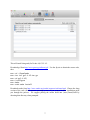
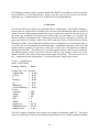
Bayesian Analysis for Stellar Evolution with Nine Parameters (BASE-9)
v9.4.3
User’s Manual
Ted von Hippel1, Elliot Robinson2, Elizabeth Jeffery3, Rachel Wagner-Kaiser4,
Steven DeGennaro5, Nathan Stein6, David Stenning7, William H Jefferys8, and
David van Dyk9
1
Embry-Riddle Aeronautical University, Daytona Beach, FL, USA; [email protected]
Argiope Technical Solutions, Ft White, FL, USA; [email protected]
3
Brigham Young University, Provo, UT, USA; [email protected]
4
University of Florida, Gainesville, FL, USA; [email protected]
5
Studio 42, Austin, TX, USA; [email protected]
6
University of Pennsylvania, Philadelphia, PA, USA; [email protected]
7
University of California, Irvine, CA, USA; [email protected]
8
University of Texas, Austin, TX, USA and University of Vermont, Burlington, VT, USA;
[email protected]
9
Imperial College London, London, UK; [email protected]
2
BASE-9 is a Bayesian software suite that recovers star cluster and stellar parameters from
photometry. BASE-9 is useful for analyzing single-age, single-metallicity star clusters, binaries,
or single stars, and for simulating such systems. BASE-9 uses Markov chain Monte Carlo and
brute-force numerical integration techniques to estimate the posterior probability distributions for
the age, metallicity, helium abundance, distance modulus, and line-of-sight absorption for a
cluster, and the mass, binary mass ratio, and cluster membership probability for every stellar
object. BASE-9 is provided as open source code on a version-controlled web server. The
executables are also available as Amazon Elastic Compute Cloud images. This manual provides
potential users with an overview of BASE-9, including instructions for installation and use.
Table of Contents I. Introduction ....................................................................................................................................... 3 II. Skip the install and go to the cloud ........................................................................................... 5 III. Installation ....................................................................................................................................... 6 A. Installing gcc, gsl, and cmake on a Mac running OS X 10.7 – 10.9 .............................................. 6 B. Installing gcc, gsl, and cmake on a Linux machine .......................................................................... 8 C. Unpacking BASE-­‐9 ...................................................................................................................................... 8 E. Installing BASE-­‐9 ........................................................................................................................................ 9 IV. Running BASE-­‐9 .............................................................................................................................. 9 A. simCluster .................................................................................................................................................. 10 B. scatterCluster ............................................................................................................................................ 11 C. singlePopMcmc ......................................................................................................................................... 13 D. sampleMass and sampleWDMass ....................................................................................................... 15 E. makeCMD .................................................................................................................................................... 16 F. Hyades Test ................................................................................................................................................ 17 G. How long does all of this take? ............................................................................................................ 17 V. Diagnostics of run quality ........................................................................................................... 18 VI. Example uses of BASE-­‐9 ............................................................................................................. 19 VII. Modifying the code to extend its capabilities ................................................................... 22 2 I. Introduction
Bayesian Analysis for Stellar Evolution with Nine Parameters (BASE-9) is a Bayesian software
suite that recovers star cluster and stellar parameters from photometry. BASE-9 is useful for
analyzing single-age, single-metallicity star clusters, binaries, or single stars, and for simulating
such systems. This document assumes you are working with base 9.4.3. We will endeavor to
update this manual as we update the code or as libraries or operating systems meaningfully
change.
BASE-9 uses a Markov chain Monte Carlo (MCMC) technique along with brute-force numerical
integration to estimate the posterior probability distribution for up to six cluster and three stellar
properties. The cluster properties are age, metallicity, helium abundance, distance modulus, lineof-sight absorption, and parameters of the initial-final mass relation (IFMR). The stellar
properties are primary mass, secondary mass (if a binary), and cluster membership probability.
The MCMC technique is used for the cluster quantities and numerical integration is used for the
stellar quantities. BASE-9 is freely available source code that you may use as is or modify for
your own research and educational purposes.
BASE-9 may be the code for you if
1. you are dissatisfied with deriving cluster-level parameters by over-plotting isochrones on
your data and iteratively adjusting parameters,
2. you wish to recover more than just an average and error bar for each parameter, and
instead wish to characterize the probability distributions for these parameters,
3. you wish to take fuller advantage of ancillary data, such as proper motion membership
probabilities, spectroscopic mass estimates, or distances from trigonometric parallaxes.
This manual is designed to help you install and run BASE-9. If you use BASE-9 in your
research, please cite
von Hippel, T., Jefferys, W. H., Scott, J., Stein, N., Winget, D. E., DeGennaro, S., Dam, A.,
& Jeffery, E. 2006, Inverting Color-Magnitude Diagrams to Access Precise Star Cluster
Parameters: A Bayesian Approach, ApJ, 645, 1436
and if you find the following helpful, please also cite
DeGennaro, S., von Hippel, T., Jefferys, W. H., Stein, N., van Dyk, D. A., & Jeffery, E.
2009, Inverting Color-Magnitude Diagrams to Access Precise Star Cluster Parameters: A
New White Dwarf Age for the Hyades, ApJ, 696, 12
van Dyk, D. A., DeGennaro, S., Stein, N., Jefferys, W. H., & von Hippel, T. 2009, Statistical
Analysis of Stellar Evolution, Annals of Applied Statistics, 3, 117
Depending on how you use BASE-9 (this part is under your control), the software also relies on
the stellar evolution models of
Dotter, A., Chaboyer, B., Jevremovic, D., Kostov, V., Baron, E., & Ferguson, J. W. 2008,
The Dartmouth Stellar Evolution Database, ApJS, 178, 89
3 Girardi, L., Bressan, A., Bertelli, G., & Chiosi, C. 2000, Evolutionary tracks and isochrones
for low- and intermediate-mass stars: From 0.15 to 7 Msun, and from Z=0.0004 to 0.03,
A&AS, 141, 371
Yi, S., Demarque, P., Kim, Y.-C., Lee, Y.-W., Ree, C. H., Lejeune, T., & Barnes, S. 2001,
Toward Better Age Estimates for Stellar Populations: The Y2 Isochrones for Solar Mixture,
ApJS, 136, 417
the white dwarf atmosphere models of
Bergeron, P., Wesemael, F., & Beauchamp, A. 1995, Photometric Calibration of Hydrogenand Helium-Rich White Dwarf Models, PASP, 107, 1047
(as updated and made available at http://www.astro.umontreal.ca/~bergeron/CoolingModels/)
the white dwarf interior models of
Althaus, L. G. & Benvenuto, O. G. 1998, Evolution of DA white dwarfs in the context of a
new theory of convection, MNRAS, 296, 206
Montgomery, M. H., Klumpe, E. W., Winget, D. E., & Wood, M. A. 1999, Evolutionary
Calculations of Phase Separation in Crystallizing White Dwarf Stars, ApJ, 525, 482
(The paper describes the stellar evolution code that M. Montgomery used in 2012 to calculate
the WD sequences specifically for use with BASE-9.)
Renedo, I., Althaus, L. G., Miller Bertolami, M. M., Romero, A. D., Corsico, A. H.,
Rohrmann, R. D., & Garcia-Berro, E. 2010, New Cooling Sequences for Old White Dwarfs,
ApJ, 717, 183
Wood, M. A. 1992, Constraints on the age and evolution of the Galaxy from the white dwarf
luminosity function, ApJ, 386, 539
the Initial Mass Function of
Miller, G. E., & Scalo, J. M. 1979, The initial mass function and stellar birthrate in the solar
neighborhood, ApJS, 41, 513
and the Initial-Final Mass Relations of
Salaris, Salaris, Maurizio; Serenelli, Aldo; Weiss, Achim; Miller Bertolami, Marcelo. 2009,
Semi-empirical White Dwarf Initial-Final Mass Relationships: A Thorough Analysis of
Systematic Uncertainties Due to Stellar Evolution Models, ApJ, 692, 1013
Weidemann, V. 2000, Revision of the initial-to-final mass relation, A&A, 363, 647
4 Williams, K. A., Bolte, M., & Koester, D. 2009, Probing the Lower Mass Limit for
Supernova Progenitors and the High-Mass End of the Initial-Final Mass Relation from White
Dwarfs in the Open Cluster M35 (NGC 2168), ApJ, 693, 355
or a fitted IFMR parameterized as lines, broken lines, or low-order polynomials as described by
Stein, N. M., van Dyk, D. A., von Hippel, T., DeGennaro, S., Jeffery, E. J., & Jefferys, W. H.
2013, Combining Computer Models in a Principled Bayesian Analysis: From Normal Stars
to White Dwarf Cinders, Statistical Analysis and Data Mining, 6, 34
For a further discussion of what BASE-9 and its precursor, BASE-8, has been used for to date
and some indications of how it might be useful in your research, see also the following papers:
Jeffery, E. J., von Hippel, T., Jefferys, W. H., Winget, D. E., Stein, N., & DeGennaro, S.,
2007, New Techniques to Determine Ages of Open Clusters Using White Dwarfs, ApJ, 658,
391
Jeffery, E. J., von Hippel, T., DeGennaro, S., Stein, N, Jefferys, W.H., & van Dyk, D. 2011,
The White Dwarf Age of NGC 2477, ApJ, 730, 35
II. Skip the install and go to the cloud
BASE-9 executables are available as Amazon Elastic Compute Cloud (EC2) images. Up-to-date
instance IDs are listed in the release descriptions at http://github.com/argiopetech/base/releases.
An Amazon Web Services (AWS) account is required to use these instances.
To run your code on EC2, 1. Log in to your AWS account 2. Navigate to EC2 3. Navigate to the “Instances” pane 4. Click “Launch Instance” 5. Choose “Community AMIs” 6. Enter the AMI code for the version of BASE-9 you would like to run 7. Select “Review and Launch”, then “Launch” 8. Wait for the instance to launch 9. use rsync/scp to copy your data to the public IP of the instance 10. Login to your instance with SSH The default user name is ec2-­‐user. There is no root password by default. BASE-9 executables are in /usr/local/bin (should be in the path). Current models
(appropriate for the installed version of BASE-9) are in /usr/local/share/base-­‐models. The instance operating system is the newest release of FreeBSD 10. The tcsh, csh, sh, and bash
shells are available. VI, VIM, Emacs, and nano are pre-installed. 5 III. Installation
BASE-9 is written in C++ and designed to run on a variety of UNIX- and Linux-based operating
systems. It is currently tested on
•
•
•
•
•
Mac OS X 10.7 through 10.9
Ubuntu 10.04 through 12.04
RHEL 5 and 6
Gentoo 13.0
FreeBSD 9 and 10
To compile the code you will need gcc 4.7+ or clang 3.2+ (C/C++ language compilers), gsl (the
gnu science library), cmake (a cross-platform build system), and Boost (a peer-reviewed,
portable C++ library). To install these software packages, you may need help from your system
administrator, though we provide some guidance here.
The best place to put all of this code is in the /usr/local/bin directory. If you don’t have that
directory on your machine already, you can create it as follows:
> sudo mkdir /usr/local > sudo mkdir /usr/local/bin
Note that the sudo command gives you super-user or root permission for that one command
(after you enter your password at the prompt), assuming that your account has been allowed to
invoke the command.
A. Installing gcc, gsl, and cmake on a Mac running OS X 10.7 – 10.9
Download the compiler. One way to do that is via downloading Xcode 4.6 or later from
http://connect.apple.com. This requires that you have a developer account, but you can register
for that for free. Also, it will give you 1+ GB of code and tools, most of which you will only
need if you intend to develop for iPhones, Mac OS, etc. If you do follow this route, after
installing Xcode, you will need to specifically install the command line tools with a window that
will look similar to the one below. Click on the install button to the right of “command line
tools” and it will appear as follows when done.
6 This will install clang and (for Xcode 4.6) GCC 4.2.
Download gsl from http://www.gnu.org/software/gsl/. Use the ftp site to obtain the source code,
then
mac> cd ~/Downloads mac> tar xzf gsl-­‐1.15.tar.gz mac> cd gsl-­‐1.15/ mac>./configure mac> make mac> sudo make install
Download cmake from http://www.cmake.org/cmake/resources/software.html. Choose the .dmg
version of the code (for the correct operating system) if you want to let Mac installation guide
you through the process. We suggest placing the cmake build into /usr/local/bin by
choosing that directory when prompted.
7 B. Installing gcc, gsl, and cmake on a Linux machine
The simplest way to install on Ubuntu is via the apt-get tool.
linux> sudo apt-­‐get install gcc linux> sudo apt-­‐get install cmake cmake-­‐curses-­‐gui linux> sudo apt-­‐get install libgsl0-­‐dev libgsl0ldbl
A similar process will work with the yum tool on Fedora / RHEL* :
linux> sudo yum install gcc gcc-­‐c++ cmake git linux> sudo yum install gsl gsl-­‐devel boost boost-­‐devel *RHEL 5 & 6 repositories have an old gcc version. The devtoolset package will install an
alternate, up to date build environment at /opt/<distro>/devtoolset-2/
linux> sudo yum install devtoolset-­‐2-­‐toolchain The scl utility can create a shell referencing these alternate build tools where BASE-9 can be
built:
linux> scl enable devtoolset-­‐2 'bash' C. Unpacking BASE-9
Create a directory where you wish to install and run the software, then download the newest code
release from https://github.com/argiopetech/base/tags and the newest stellar evolution files from
https://github.com/argiopetech/base-models/tags, and extract them to the appropriate directory,
e.g.
> tar xzf base-­‐9.4.2.tar.gz > cd base-­‐9.4.2/
Note that your computer may uncompress the .gz file for you on download, in which case the
above command would instead be
> tar xvf base-­‐9.4.2.tar > cd base-­‐9.4.2/
8 D. Installing Boost
BASE-9 has an included script to install Boost. The install location can be changed by modifying
the CMAKE_INSTALL_PREFIX variable.
linux> cd contrib linux> cmake –DCMAKE_INSTALL_PREFIX=”/usr/local” . linux> sudo make
Ubuntu users can save some time on this step by running
linux> sudo apt-­‐get install libboost-­‐dev E. Installing BASE-9
Once you have all of the above software in place, you are ready to install BASE-9. The
following instructions should work identically for all platforms.
Change directories into the BASE-9 source directory and simply run build.sh
> sudo ./build.sh This will (if you have properly installed all libraries) build and install the BASE-9 executables
and install them in the default location (generally /usr/local/bin)
Alternatively, if you do not have the ability to run `sudo` on your machine, you may use
> ./build_local.sh to build and install the executables locally. The executables will be installed in the BUILD/bin
directory.
IV. Running BASE-9
In the following subsections, we describe how to run stand-alone portions of the BASE-9
modules from the command line. There are various reasons why you might want to run one or
another of these, or some, but not all, so we detail how to run each one. As of BASE-9.2.0, all
settings have been moved into a YAML-format configuration file. A sample configuration file
with reasonable initial settings can be found in the base-­‐9.4.2/conf directory under the name
base9.yaml. A sample cshell script can be found at scripts/hyades.csh. Individual
settings can be changed on a run-by-run basis via the command line options. Run any of the
BASE-9 applications with the command line flag “--help” to view a description of available
settings.
9 The following examples assume you have installed the BASE-9 executables in a directory that is
in your PATH (e.g., /usr/local/bin). If this is not the case, you may need to use absolute
pathnames (e.g., /home/me/base-­‐9.4.2/BUILD/bin/singlePopMcmc).
A. simCluster
The first tool that you are likely to use within BASE-9 is simCluster. This module simulates a
stellar cluster for a particular set of models (see references in the Introduction) and user-specified
values of various cluster parameters that have been set in the base9.yaml file: the base-10 log of
the cluster age, metallicity, the helium mass fraction (only for some Dotter et al. models), the
distance modulus, absorption in the V-band, the percent of cluster stars that are binaries, the
upper mass limit for creating a white dwarf (WD), and the fraction of WDs that have helium
atmospheres (DBs). We recommend leaving these last two parameters at 8 solar masses and 0%,
as we have not yet fully implemented and tested them. An additional parameter, the seed to the
random number generator, is necessary as the mass of each star is determined by randomly
drawing from the IMF. This allows you to specify multiple clusters with the same parameters
but different random seeds if you wish to test the effects of, for instance, cluster size on the
number of WDs or the clarity of the main sequence turn-off (MSTO). This seed can be set via
the -­‐-­‐seed option in the command line. To run simCluster, simply type its name:
linux> ./simCluster Seed: 1559729633 Reading models... Done. Properties for cluster: logClusAge = 8.796 [Fe/H] = 0.07 Y = 0.29 modulus = 0.00 Av = 0.01 WDMassUp = 8.0 fractionBinary = 0.00 Totals: nSystems = 100 nStars = 100 nMSRG = 98 nWD = 2 nNSBH = 0 massTotal = 62.72 MSRGMassTotal = 55.10 wdMassTotal = 1.66 The above output is diagnostic and reiterates the settings in the base9.yaml file. The stored
output of simCluster is placed in a filename specified by the user with the outputFileBase
10 option in the base9.yaml file. The file contents from the output of simCluster should look
like the following:
linux>head -­‐2 hyades.sim.out id U B V R I J H K sigU sigB sigV sigR sigI sigJ sigH sigK mass1 massRatio stage Cmprior useDBI 1 3.061 3.031 2.694 2.501 2.320 2.127 1.983 1.965 0.000 0.000 0.000 0.000 0.000 0.000 0.000 0.000 1.555 0.000 1 0.999 1 There are more columns than can be presented cleanly on a page, but hopefully this is clear
enough. The first column lists identification numbers for each star system (single star or binary).
This is meant to be useful in tracking down particular stars. The next eight columns list the Uthrough K-band magnitudes (or ugriz through K) of the primary star. Columns 10 through 17
give the photometric uncertainties for each filter entry (for a simulated cluster, these are zero).
The 18th and 19th columns give the mass of the primary star and the mass of its companion (if
applicable). The 20th column lists the stage of stellar evolution for that particular star (1 = MS
or RG, 3 = WD, >3 for evolved stars above the WD mass limit). The final two columns are the
cluster membership prior (which is essentially ~1 for simulated stars) and the flag (0 or 1)
whether to use the star during the burn-in stage. With these final columns, the output file is
formatted for input into scatterCluster. You should be able to plot reasonable looking
CMDs/isochrones from this file for a wide range of cluster parameters, stellar models, and filters.
B. scatterCluster
The scatterCluster module adds Gaussian random errors to the photometry output created
by simCluster. To specify the appropriate amount of error to add for your particular
simulation, adjust the virtual exposure time in the base9.yaml file.
We use exposure times of 1 hour in each filter to generate a scattered cluster with the above file.
The algorithm for adding noise to the cluster photometry is rudimentary and only meant for
simple purposes such as preparing for an observing proposal or for creating test files for the
Markov chain Monte Carlos (singlePopMcmc) routine. The algorithm is an approximation to
the results one would obtain in one hour with the KPNO 4m + Mosaic (UBVRI) or Flamingos
(JHK), assuming dark time, seeing=1.1 arcsec, airmass=1.2. Signal-to-noise for the Spitzer
bands, if included, are naively set to be the same as for the K-band. For departures from a onehour exposure the S/N is scaled by sqrt(exptime). These exposure times can be set in the
base9.yaml file under exposures for each individual filter.
Additional options for scatterCluster are available in the yaml file. The bright and faint end
cut-off mags allow you to narrow the portion of the CMD that you wish to retain. The
relevantFilt option specifies which band is the reference filter (in this case, 0=U, 1=B, etc.).
The base9.yaml options brightLimit and faintLimit refer to the bright and faint end cut 11 off magnitudes for the reference filter indicated. You can also clip on S/N with limitS2N and
decide to cut out field stars, if they were simulated by simCluster. Additionally,
scatterCluster will determine which filters you are using based on the header in the
simCluster output file. Again, the integer seed may be set at the command line to allow you
to start from the same input file, but create multiple simulated observations of that file with
different initial seed values.
linux> scatterCluster Seed: 1564704505 The output file of scatterCluster looks like
linux> head -­‐2 hyades/hyades.scatter.out id U B V R I J H K sigU sigB sigV sigR sigI sigJ sigH sigK mass1 massRatio stage Cmprior useDBI 1 3.065 3.016 2.691 2.509 2.328 2.128 1.985 1.977 0.010 0.010 0.010 0.010 0.010 0.010 0.010 0.010 1.555 0.000 1 0.999 1 Notice now that the output includes the estimated errors for each band (sig-­‐). The format of the
output file is otherwise the same as the input file for scatterCluster.
In this case, only the id, mass1, and stage1 values are kept from the output of simCluster.
The photometry values (here UBVRIJHK) are derived from the photometry values in the
simCluster output file, but are different in that they are scattered by adding a Gaussian random
deviate with sigma = sigU, sigB, etc. This section of the output file is all one needs to plot
realistic CMDs for proposals and possibly to prepare for observing projects.
The
scatterCluster output file contains additional information, however, and is formatted to be
ingested by singlePopMcmc, so that it can be used to test singlePopMcmc and so that you can
test the precision and accuracy that you would expect to recover from real data based on a given
set of cluster parameters, observational errors, and the number of stars available. The
massRatio column lists the ratio by mass of the secondary to primary stars, which in these
examples are both 0 since there were no secondaries. The CMprior column is set by default in
scatterCluster to 0.99, but the file can easily be edited to set a different prior probability
that any particular star is a cluster member. The final column is just a 0 or 1 switch (off or on) of
whether to use a particular star during the burnin process. (See DeGennaro et al. 2009 and van
Dyk et al. 2009 for a discussion of what the burnin entails and why it is used.) To make it easiest
for singlePopMcmc to converge, it is helpful to have this parameter set to 1 for stars that are
likely to be cluster members and if there are many field stars, it is helpful if the bulk of them can
be set to 0 at this point.
12 C. singlePopMcmc
The singlePopMcmc module is the workhorse of our software suite. This routine, along with
its many subroutines, runs a Markov chain Monte Carlo sampler using a variety of standard
Bayesian techniques as well as a few techniques newly developed by us. The approach and
mathematics are presented by DeGennaro et al. (2009), van Dyk et al. (2009), and Stein et al.
(2013). This code was designed to run on photometry formatted in the same manner as the
output of scatterCluster. It can also be run just as easily on the simulated photometry from
simCluster + scatterCluster.
The singlePopMcmc module has a variety of values and options set in the base9.yaml file.
Under the singlePopMcmc group, the stage2IterMax and stage3Iter set the length of the
burnin for singlePopMcmc. The runIter option lets you choose the number of iterations of
the Markov chain Monte Carlo. The rule-of-thumb is that one typically wants 10,000 wellsampled points from a Markov chain Monte Carlo in order to draw robust inferences on the
posterior distribution. At the other extreme, the Central Limit Theorem dictates that
approximately 30 uncorrelated samples are sufficient for a normal distribution. Before running a
particular dataset against a specific set of models, you do not know if the posterior distributions
will be Gaussian shaped or more complex, so we suggest you take the conservative approach and
initially assume complex posterior distributions and run BASE-9 for 10,000 uncorrelated
iterations. The parameter thin sets the increment between saved iterations. We recommend
that this parameter be left equal to 1 to keep the adaptive sampling routine efficient. If the output
of singlePopMcmc is correlated (see below), then each new iteration or step is not independent
and you need substantially more than 10,000 iterations to draw robust inferences. In situations
like this, we recommend that the output file be thinned afterwards, i.e. that the user uses every nth
record where n is large enough to keep the output uncorrelated.
Under the cluster options, there are five parameters for which means and standard deviations
can be set: the metallicity prior (Fe_H), the distance modulus prior (distMod), the absorption
prior (Av), the helium prior (Y), and the carbon fraction prior for a C+O WD (carbonicity).
Note that carbonicity only works with the Montgomery models and is not yet supported
because we are currently testing it. If you only have weak priors, that is fine. If you do not want
to sample on one or more of these parameters, you can set the sigma for that parameter to 0.0
and this will turn of sampling for that parameter. Under starting, the parameter logClusAge
is a starting value for the log of the age in years (e.g. 9.0 for a 1 billion year old cluster). This is
not a prior, but just tells singlePopMcmc where to start searching for a fit. We have found that
although convergence may depend on starting with a roughly reasonable age, the actual posterior
age distribution does not depend on what that value is, assuming it does converge.
The msRgbModel lets you choose which set of models to use with your data (the filters available
in the models must match the filters of your observed or simulated/scattered cluster). This
allows you to derive cluster parameters for a range of models as well as to create simulated
clusters under one set of models and use singlePopMcmc to derive the cluster and stellar
parameters under another set of models. The latter experiments might be useful, for instance, if
you wanted to test the sensitivity of basic cluster or stellar parameters to a given model
13 ingredient. With ancillary data for cluster or stellar parameters this might allow you to constrain
model ingredients.
Again we mention that the seed can be set inline with -­‐-­‐seed when singlePopMcmc is called.
If singlePopMcmc appears to be unable to converge on reasonable cluster values, rerun it with
a different initial seed. Changing the seed also allows you to start a new MCMC chain if you ran
a prior calculation with too few iterations.
To run singlePopMcmc, using a properly prepared input base9.yaml file, type the following:
linux> singlePopMcmc -­‐-­‐verbose Bayesian Analysis of Stellar Evolution Seed: 1570065938 Reading models... Done. Model boundaries are (7.800, 10.250) log years. Binaries are OFF Running Stage 1 burnin... Complete (acceptanceRatio = 0.090) Running Stage 2 (adaptive) burnin... Acceptance ratio: 0.350. Trying for trend. Acceptance ratio: 0.600. Retrying. Acceptance ratio: 0.380. Trying for trend. Acceptance ratio: 0.520. Retrying. Acceptance ratio: 0.280. Trying for trend. Acceptance ratio: 0.180. Retrying. Acceptance ratio: 0.400. Trying for trend. Acceptance ratio: 0.440. Retrying. Acceptance ratio: 0.320. Trying for trend. Acceptance ratio: 0.500. Retrying. Acceptance ratio: 0.240. Trying for trend. Leaving adaptive burnin early with an acceptance ratio of 0.220 (iteration 1300) Starting adaptive run... Preliminary acceptanceRatio = 0.300 The singlePopMcmc routine creates multiple output files. In this case, it created:
-­‐rw-­‐r-­‐-­‐r-­‐-­‐ 1 comp staff 57955 Nov 3 17:27 hyades/hyades.res -­‐rw-­‐r-­‐-­‐r-­‐-­‐ 1 comp staff 50317 Nov 3 17:25 hyades/hyades.res.burnin The .burnin files provide the sampling patterns during the burnin process and may be useful
for diagnostic purposes, especially if singlePopMcmc is not sampling well (see below). The
.res.burnin files look like:
14 linux> head -­‐2 hyades/hyades.res.burnin logAge Y FeH modulus absorption logPost 8.821886 0.280626 0.086646 -­‐0.010790 0.011206 -­‐174.520334 And the .res files have the same format: linux> head -­‐2 hyades/hyades.res logAge Y FeH modulus absorption logPost 8.843553 0.288468 0.016795 -­‐0.180626 0.013647 -­‐198.263339 After the column headers, there is one record for each iteration of each of the cluster parameters
of interest.
If everything goes well, all you really need to do is plot histograms for any column of interest.
These are the posterior parameter distributions. You can also calculate moments of these
columns if you’d like, and look at correlations among the columns, e.g. by plotting logAge vs.
modulus.
D. sampleMass and sampleWDMass
These modules are useful for anyone interested in the masses of some or all of the stars in their
database. Running them is unnecessary if you are only interested in the cluster parameters. The
module sampleMass reports the primary mass and secondary mass ratio at all iterations for
every star in the database, and sampleWDMass reports the primary mass for the subset of
database stars that are being fit as WDs.
Running these programs is quite simple:
linux> sampleWDMass Seed: 1690745648 Warming up generator… Done. Generated 10000 values. Reading models… Done. sampledPars.at(0).age = 8.78411 sampledPars.at(last).age = 8.74765 Part 2 completed successfully Running sampleMass is effectively identical.
These output files names end with .wdMassSamples, .wdMassSamples.membership,
.massSamples, and .massSamples.membership. These correspond to the WD mass
outputs from sampleWDMass, the membership likelihood of those masses, the mass and
secondary mass ratio outputs from sampleMass, and the membership likelihood of those pairs.
15 sampleWDMass output files consist of the same number of columns as there are WDs, and the
same number of rows as there are in the results (.res) file. Each item in a row corresponds to
the mass of a WD (ordered as in the database) given the sampled parameters in the results file.
The membership file shares this format, though the values correspond to the likelihood that the
given star is a member of a cluster with the given parameters.
sampleMass output files are similar to sampleWDMass output files but have two columns per
star in the database. For every 0-indexed star 𝑘 in the database, column 2𝑘 corresponds to that
star’s primary mass, and 2𝑘 + 1 to that star’s secondary mass ratio. The membership file is
identical to that of sampleWDMass, though the values correspond to the likelihood that the given
unresolved binary is a cluster member.
sampleWDMass has no configurable parameters.
sampleMass takes two parameters in the YAML file: deltaMass and deltaMassRatio.
These values are used as starting step sizes for the adaptive MCMC process used to obtain mass
and mass ratio. We recommended that you change these parameters only if you are manipulating
the code for diagnostic purposes.
E. makeCMD
The final module of our software suite, makeCMD, is a small module that calculates a mean fit
isochrone. This is helpful for runs that do not converge as well as for situations where the
posterior distribution of some key parameter may be multimodal. To run makeCMD
linux> makeCMD Seed: 1574116425 Reading models... Done. ***Warning: "F435W" is not available in the selected WD Atmosphere model This is non-­‐fatal if you aren't using the WD models The output of makeCMD looks like
linux> head -­‐2 hyades/hyades.cmd Mass U B V R I J H K F435W F475W F550M F555W F606W F625W F775W F814W 0.150000 16.170454 14.623905 13.035403 11.950929 10.490719 9.196773 8.640356 8.386555 14.666132 13.907510 12.768529 13.128038 12.587469 12.243942 10.744691 10.477001 Because makeCMD uses the values of means under cluster in the base9.yaml, one can enter
the mean or median values from the singlePopMcmc posterior distributions into the yaml file
16 prior to running makeCMD. The output file from makeCMD can then be used to overplot what
essentially amounts to the average fit isochrone from among the posterior parameter
distributions. Note that this is not a best-fit isochrone, but rather a representative example drawn
from that distribution. In fact, isochrones created from summary statistics such as mean or
median parameters may not be truly representative if the distributions are substantially nonGaussian because that simultaneous combination of parameters may fit the data with low
probability.
F. Hyades Test
We have created a script, hyades.csh, which is set up to run on a Hyades data set
(Hyades.UBV.testphot). It is a cshell script. If you have problems with this script, you may
be using a shell other than the cshell or tshell, e.g. the Bourne shell. You can invoke the cshell as
follows:
Bourne shell> csh New prompt indicating you are now running csh> hyades.csh This will allow you to test your code installation and plot results, then compare to the
DeGennaro et al. results. Note that you will not obtain an exact correspondence to the results of
DeGennaro et al. because we have updated the Hyades data set since that publication. Because
of the relative depth of the Hyades, which is significant compared to its distance, we have now
corrected the cluster stars to lie at the mean cluster distance using individual proper motions
from Hipparcos and the cluster converging point method. Because of the way we have corrected
distances, this data set is converted to absolute magnitude space (we otherwise always use
apparent magnitudes) and for this one test case, you will find a distance modulus of
approximately 0.0.
G. How long does all of this take?
In our tests, it took 147 minutes to run hyades.csh, which in turn ran singlePopMcmc for 152
Hyades stars in three photometric bands for 10,000 iterations on a early 2011 Macbook Pro (2.3
GHz Intel with 8 GB RAM) laptop computer. Increasing the number of filters or number of stars
will increase the computation time linearly. Increasing the number of MCMC iterations will
increase the run time, but somewhat less than linearly because some of the time is spent during
the burnin. You will see substantial increases in runtime if you have much larger data sets and/or
if you have to increase the total number of calculated iterations.
17 V. Diagnostics of run quality
The following two plots show examples of poor and good sampling. In the first (extreme) case,
the age sampling is highly correlated and one would need to use post-run thinning, probably by a
factor of ~100. This means that one would need to run the code for 100x as many interations.
The metallicity sampling displays only minor correlation, and if all other parameters looked this
uncorrelated then this run would be sufficient. In this particular case, both plots were generated
from the same singlePopMcmc run and because no single parameter is reliable until all
parameters are essentially uncorrelated, this run did not reliably determine the metallicity (or any
other) posterior distribution.
18 VI. Example uses of BASE-9
In Section IV we outlined how to use the outputs of BASE-9. Here we provide additional
examples from our papers and on-going work.
The first figure of this section, taken from DeGennaro et al. (2009), shows Hyades CMDs with
three sets of stellar evolution models placed at their average fit values as determined by a
previous version of the code, BASE-8. Because these stellar models do not provide good fits to
the lower main sequence, the following figure shows the derived age from BASE-8 for each of
the three input models and for a range of lower main sequence cut-offs. In this way DeGennaro
et al. were able to argue that their derived parameters were stable over an appropriate range of
data and were able to quantitatively point to where problems emerged in the models.
19 This next figure, taken from Jeffery, E. J. (2009, Ph.D. Dissertation, University of Texas at
Austin) compare the age information resident in just the main sequence turn-off stars (black
dashed line) compared to that resident in the white dwarfs. Data from the main sequence was
included in both BASE-8 runs, and this provides the primary constraints on metallicity, distance,
and reddening. This is useful for studying the information content in the MSTO vs. WD regions.
20 The next figure, also from Jeffery (2009), indicates how one can study the sensitivity of a given
result to the observations of an individual star. For the open cluster NGC 2360, the posterior age
distribution is given by the black line. During some iterations, however, a particular WD is fit as
a field star and the remaining WDs yield the posterior age distribution indicated in red. During
the iterations when this particular WD is included in the fit, the posterior age distribution is as
indicated in blue. The final age posterior distribution is a linear combination of these two
distributions based on the fraction of time this particular WD was included in the fit.
The next figure shows unpublished work based on applying BASE-8 to an individual WD. In
this particular case, we know that the WD has a hydrogen atmosphere (type DA), yet for
demonstration purposes we analyze it both as a DA and as a DB (helium atmosphere). We also
try two different initial-final mass relations (from Salaris et al. 2009 and Williams, Bolte, &
Koester 2009). The clouds of points show acceptable fits and the error bars indicate the mean
and standard deviation for each of the four cases. Clearly these distributions are non-Gaussian
and publishing just the means and standard deviations could lead readers to misunderstand the
results. This kind of analysis can also point the way toward future observational work. For this
star a trigonometric parallax could potentially rule out much of the age range, yielding a precise
age. If this star were a DB a much more accurate trig parallax would be required to
meaningfully constrain the age. This is not a general statement about WDs, but a result for this
star with the available photometry (grizJHK).
21 VII. Modifying the code to extend its capabilities
We continue to upgrade BASE-9 for our on-going projects. If you wish to add capability to
BASE-9, we will be happy to suggest to you how best to go about this and try to estimate the
work involved. Here is an example list of how involved a variety of tasks are likely to be.
Less than 2 hours: Modifying the IFMR. You can do this by editing or adding a few lines of
code in ifmr.cpp.
Less than 8 hours: Change the IMF. You will need to create a subroutine where a random mass
value can be drawn from your IMF distribution.
This currently takes place in
drawFromIMF.cpp. Note that you will also have to normalize the IMF for the Bayesian routine
to work properly and that this takes place in densities.cpp and is stored in logMassNorm.
Less than 16 hours: Incorporating another set of stellar evolution models – see instructions at the
top of msRgbEvol.cpp and possibly wdCooling.cpp and/or gBergMag.cpp.
Less than a week: Sampling a new variable (e.g. stellar rotation, alpha-element enhancement).
This takes place primarily in singlePopMcmc/MpiMcmcApplication.cpp and
base9/densities.cpp.
22