Download Entanglement and Bell`s Inequalities

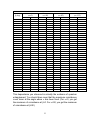
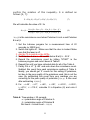
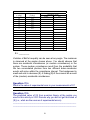
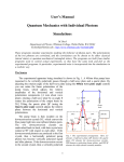
UNIVERSITY OF ROCHESTER
THE INSTITUTE OF OPTICS
OPT 453, OPT 253, PHY 434
Lab. 1. Entanglement and
Bell’s Inequalities
Instructor: Dr. Svetlana G. Lukishova
[email protected]
Fall 2008
“I cannot seriously believe in quantum theory because it cannot be reconciled with the idea that
physics should represent a reality in time and space, free from spooky actions at a distance." Albert Einstein
Summary of this Lab
•
Entanglement is the most exciting and mysterious property of some
quantum mechanical systems when property of one particle depends on
the property of the other. It does not matter how far apart such entangled
particles are located. Among the best known applications of entanglement
are quantum communication and quantum state teleportation.
•
Bell’s inequality is a classical relation. For entangled particles it is violated.
•
In this lab you will obtain an entangled state of two photons and will
calculate Bell’s inequality using measurements of the coincidence counts
between two single-photon detectors. You will work on modern, cutting
edge photon counting instrumentation widely used in quantum information
science and engineering. The table below shows its other applications.
Photon counting applications
bioluminescence
single molecule
detection
detector
calibration
primary
radiometric
scales
quantum
standards
quantum
cryptography
hyper-spectral
imaging
medical imaging
Metrology
lighting
photon
count
Electronics
quantum
computing
Quantum
Information
Processing
Biotechnology
displays
quantum
imaging
single photon
sources
Medical
Physics
medical / non
interactive
imaging
entertainment
neutrino/
cherenkov/ dark
matter detection
Space
Applications
radioactivity
Military
Meteorology
nuclear
night vision
IR detectors
robust imaging
devices
lidar
remote sensing
environmental monitoring
security
chemical – bio agent detection
Areas of applications of photon counting instrumentation (prepared by organizers of
second international workshop “Single Photon: Sources, Detectors, Applications and
Measurements Methods” (Teddington, UK, 24-26 October 2005))
2
IMPORTANT SAFETY TIPS
A. LASER SAFETY
The argon ion laser BeamLok 2060 emits laser radiation that can permanently
damage eyes and skin. To minimize the risk of injury or expensive repairs,
carefully follow these instructions.
PRECAUTIONS FOR THE SAFE OPERATION
OF CLASS IV-HIGH POWER LASERS
•
Wear protective eyewear at all times; selection depends on the wavelength
and intensity of the radiation, the conditions of use, and the visual function
required. During the alignment of your setup you can reduce the power of the
laser.
•
Avoid looking at the output beam; even diffuse reflections are hazardous.
•
Avoid blocking the output beam or its reflection with any part of your body.
•
Try to maintain a high ambient light level in the laser operation area. This
keeps the eye’s pupil constricted, thus reducing the possibility of eye damage.
•
Laser safety issue arises also from the high voltage applied to the tube
with the argon.
B. EQUIPMENT SAFETY
For the safety of the equipment,
•
NEVER TURN ON THE ROOM LIGHTS WHILE THE APDs AND EMCCD-CAMERA ARE ON.
•
(1) After turning off the power switch always unplug the APD’s before
turning on the lights for the long period of time. (2) Also, make sure your
Lab View program is turned off before turning on the lights.
•
If APD count rate will exceed 200,000 counts/sec, reduce laser
power or put the screen in front of APD.
DON’T SWITCH OFF APD UNDER A HIGH COUNT RATE!!!!
•
Don’t turn on the BeamLok 2060 argon ion laser without water cooling
(see instructions in Appendix I of this Manual).
•
Keep water running during ~15 min after the laser turning off.
3
PREPARATORY QUESTIONS
You should answer two sets of questions:
(1) before your first laboratory session and
(2) after each section of this Manual. All questions have a blue-color
font.
Answer these questions before your first
laboratory session
1. What is entanglement? How will you create polarization
entangled photons in this experiment?
2. How will you prove in your experiment that you have entangled
photons?
3. What is spontaneous parametric down conversion?
4. Make a sketch of your experimental setup and describe its main
components.
5. For what purpose do you need a quartz plate?
6. What are single photon counting avalanche photodiode
modules? How to work with them without damaging these
detectors?
7. What are Bell’s inequalities? Can you calculate them for some
classical objects?
4
References and recommended literature:
1. M. Fox, Quantum Optics: An Introduction, Oxford University Press, 2006.
2. A. I. M. Rae, Quantum Mechanics, IoP Publ., 2002.
3. G. Greenstein and A.G. Zajonc, The Quantum Challenge, Jones and
Bartlett Publ., Boston, 2006.
4. P.G. Kwiat, K. Mattle, H. Weinfurter, A. Zeilinger, “New high-intensity
source of polarization-entangled photon pairs”, Phys. Rev. Lett., 75, 4337
(1995).
5. D.N. Klyshko, Photons and Nonlinear Optics, New York, Gordon and
Breach, 1988.
6. P.G. Kwiat, E. Waks, A.G. White, I. Appelbaum, P.H. Eberhand,
”Ultrabright source of polarization-entangled photons”, Phys. Rev. A. 60,
R773 (1999).
7. D. Dehlinger and M.W. Mitchell, “ Entangled photons, nonlocality, and Bell
inequalities in the undergraduate laboratory”, Am. J. Phys, 70,903 (2002).
8. D. Dehlinger and M.W. Mitchell, “Entangled photon apparatus for the
undergraduate laboratory,” Am. J. Phys, 70, 898 (2002).
9. J.S. Bell, Speakable and Unspeakable in Quantum Mechanics, Cambridge
University Press, 2004.
10. J. Eberly, “Bell inequalities and quantum mechanics”, Amer. J. Phys., 70
(3), 286, March (2002).
11. M.A. Nielsen, I.L. Chuang, Quantum Computation and Quantum
Information, Cambridge University Press, 2000, pp. 111-117.y
12. N. Boeuf, D. Branning, I. Chaperot, E. Dauler, S. Guérin, G. Jaeger, A.
Muller, A. Migdall, “Calculating characteristics of noncollinear phase
matching in uniaxial and biaxial crystals”, Opt. Eng. 39(4), 1016-1024
(April 2000).
http://physics.nist.gov/Divisions/Div844/facilities/cprad/index.html#contents
13. BeamLok 2060 and 2080 Ion Lasers, User’s Manual, Spectra-Physics.
14. Model 587 Z-Lok Etalon and Model 5870 Controller, User’s Manual,
Spectra-Physics.
5
1. INTRODUCTION
The purpose of this laboratory work is to introduce students to
entanglement, one of the key concepts of quantum mechanics. While
the concept of entanglement defies the classical intuition, in this lab
you will gain a better understanding of entangled particles and
experimentally verify the predictions of quantum theory.
If two particles (A and B) are entangled, their wave functions cannot
be separated. The particles cannot be represented or talked about
individually. Any measurement performed on A would change the
state of B (and vice-versa), no matter how far apart A and B may be.
The idea is illustrated in the cartoon below. There is no classical
explanation for this phenomenon.
Entangled
Entangled
A
A
B
B
Figure 1. Cartoon of A.K. Jha and L. Elgin illustrating entanglement.
Entanglement between particles is always through some physical
property. For example, the quantum mechanical state describing
particles’ momentum, spin or polarization may be entangled. You can
read about entanglement in the books [1-3] for advanced
undergraduate and graduate students.
In this laboratory two different photons whose polarization states are
entangled will be investigated. These entangled photons are
produced in a BBO crystal [4] through a process called Spontaneous
6
Parametric Down-Conversion [5]. This lab experiment was reported
in 1999 as a research paper in Ref. 6 and developped for the
students’ lab by the authors of Refs. 7 and 8. Ref. 7 contains also
some useful historical background.
Bell’s Inequality [9-11] is a mathematical equation. “Inequalities of the
Bell type by themselves have nothing to do with quantum theory.
Contexts as different as downhill skiers and laundered socks have
been used by Meystre and Bell to demonstrate this. Although Bell
inequalities are almost tautological expressions, they have attracted
much attention because they allow one to see the experimental
consequences of alternative views of physical reality which are
conveniently labeled classical and quantum mechanics” [10].
In this lab you will calculate Bell’s Inequality predicting the maximum
value of a sum of probabilities. The probabilities involved assume a
classical correlation between two particles, whose polarization states
are measured. Violating this inequality means that these particles do,
in fact, have a quantum relationship that cannot be explained by
classical mechanics.
2. EXPERIMENTAL SET UP
As shown in the schematic diagram in Figure 2, light from a ~100 mW
pump argon ion laser with a wavelength λ = 363.8 nm and a vertical
polarization passes through a blue filter and then a quartz plate. The
blue filter removes parasite fluorescence from an argon plasma tube
that may be present in the laser beam. Quartz is a birefringent
material. When light passes through the quartz plate, a phase
difference is introduced between two polarization components. This
phase difference can be adjusted by rotating the quartz plate.
A mirror re-directs the beam through a pair of BBO crystals that are
mounted back-to-back, at 90º with respect to each other. The majority
of the laser light passes through the BBO crystals and is collected at
the beam stop or rejected by the interference filters. The downconverted photons from the BBO crystals are emitted in cones [a
horizontal and a vertical polarization cone for a beam with 45o
incident polarization (relative to the BBO optical axis)]. Down7
converted photons from the BBO crystals with wavelength 2λ = 727.6
nm are detected by a pair of single-photon counting avalanche
photodiodes (APDs) modules. The x-y position of the APDs can be
adjusted using the x-y translator. APDs are single photon detectors
that give rise to an electronic signal TTL pulse when a photon is
incident on them.
APD B
APD A
Beam
Stop
Polarizer B
Polarizer A
BBO Crystals
Mirror
Laser
Quartz
Plate
Blue
Filter
Figure 2. Schematics of experimental setup.
The APDs are kept at the same height as that of the BBO crystals.
The APDs’ positions are equidistant from the center of the crystal.
This enables these two APDs to be on two diametrically opposite
points of the downconverted cone. Data from the APDs are collected
using a Lab View interface on a computer with a counter-timer board
inside.
The interference filters with 10 nm bandwidth should be placed in
front of each APD, so that only light near 730 nm (i.e. the downconverted photons) will reach the detectors. Additionally, polarizers
are located in front of each APD, so that the polarization state of
photons reaching the detectors can be selected.
8
3. BBO CRYSTALS AND PARAMETRIC DOWNCONVERSION
Beta Barium Borate (BBO) is a negative uniaxial nonlinear crystal
with some very interesting and useful properties [12]. Crystals can be
cut for the different types of nonlinear interactions. For a type I crystal
cut, when a horizontally (vertically) polarized photon of wavelength λ
is incident on the crystal, two photons of wavelength 2λ emerge from
the crystal with vertical (horizontal) polarization (Figure 3). This
process is called spontaneous parametric down-conversion and is a
standard method used to produce polarization-entangled photons [4,
6]. The down-converted photons are emitted in a cone from the
crystal. The efficiency of this down-conversion process is only 10-10
(out of 1010 incident photons only one photon would get downconverted). For details in noncolinear phase matching conditions in
parametric down conversion (Figs. 3, 4) see paper 12.
Figure 3. Down-conversion of photon with a horizontal polarization. (For
this orientation of the crystal, photons with a vertical polarization pass
straight through).
Figure 4. Down-conversion of photon with a vertical polarization. (For this
orientation of the crystal, photons with a horizontal polarization pass
straight through).
9
Since the majority of the laser light simply passes straight through the
BBO crystals, the intensity of the down-converted photons is very low
(you will not be able to see a down-converted light with naked eye).
We will use single-photon counting avalanche photodiodes (APDs)
sensitive to observe the down-converted photons
4. PRODUCTION OF POLARIZATION ENTANGLED
PHOTONS: THEORY
The production of a polarization-entangled quantum state using type I
BBO crystals with a 45o incident polarization is explained below. The
first crystal’s optic axis and the pump beam define the vertical plane.
Due to Type-I phase matching, a vertically polarized photon going
through these crystals would get down-converted in first crystal
producing two horizontally polarized photons (Figure 5).
Signal
|V>
|H H >
s
i
Idler
Figure 5: Production of two horizontally polarized photons from one
vertically polarized photon.
Mathematically it can be represented as:
V → HsHi
Here V and H represent a horizontally- or a vertically-polarized
photon. For historic reasons, photons of a down-converted pair are
called “signal” and “idler” photons, denoted by subscripts “s” and “i,”
respectively.
10
On the other hand, a horizontally-polarized photon going through
these crystals would get down-converted in the second crystal
producing two vertical photons (Figure 6).
Signal
|VsVi>
|H>
Idler
Figure 6. Production of two vertically polarized photons from one
horizontally polarized photon.
Mathematically it can be represented as:
H → V s Vi
Now what happens if photons with 45˚ polarization are incident on a
pair of BBO crystals, as shown in Figure 7 below?
H-polarized cone
|H>+|V>
|VsVi>+|HsHi>
1 2
V-polarized cone
Figure 7. Production of polarization entangled photon pairs.
A stream of 45˚-polarized photons can be considered as a beam with
half vertically and half horizontally polarized photons. So half of the
time these photons would get down-converted in the first crystal,
producing pairs of photons with horizontal polarization, and half of the
11
time they would pass through the first crystal and would get downconverted in the second crystal, producing pairs of photons with
vertical polarization. Hence, for an incident beam of 45˚-polarized
photons, the same number of photon pairs having vertical and
horizontal polarizations will be emitted from the two BBO crystals.
Mathematically this can be represented as:
H + V
→
2
Here,
H +V
2
V sV i + H s H i
2
≡ Ψent
(1)
represents a 45˚ polarized photon.
Notice that the state Ψ cannot be factored into states purely
dependent on the signal and idler photons, i.e.: Ψ ≠ 1 s 2 i , for any
choice of 1 s and 2 i . This means that the state of one particle cannot
be specified without making reference to the other particle. Particles
related thusly are called entangled, and Ψent is called an
entangled quantum state.
If we measure the polarizations of signal and idler photons in the H,
V basis, there are two possible outcomes: both vertical and both
horizontal. Each occurs half of the time. We could instead measure
the polarizations with polarizers rotated by an angle α. We use the
rotated polarization basis
(2)
Vα = cos α V − sin α H ,
H α = sin α V + cos α H
Here Vα
describes a state with polarization rotated by α from the
vertical, while H α describes a state with polarization rotated by α
from the horizontal. In this basis the entangled state is
ψ ent=
1
2
(Vα
s
Vα i + H α
s
Hα
i
(3)
Clearly, if we measure in this rotated basis, we obtain the same
results: half of the time both are Vα and half of the time both are
H ε . Knowing this, we can measure the signal polarization and infer
with certainty the idler polarization.
12
From Figure 7 you can see that a horizontal photon travels a larger
distance inside the BBO crystals than a vertical photon before getting
down-converted. This difference in distances traveled introduces a
phase difference, φ , between the two polarization states, resulting in
a quantum state:
Ψ = V sVi
+
e iφ H s H i
(4)
If the incident (pump) laser beam has a polarization angle θ from the
vertical (see Figure 8 in which the crystal optical axis is parallel to the
vertical direction), in general case the downconverted photons
emerge in the state
ψ DC = cos θ H
s
H
i
+ exp[iφ ] sin θ V
s
V
i
(5)
Figure 8. Geometry of a downconversion process.
By placing polarizers rotated to angles α and β in the signal and idler
paths, respectively, we measure the polarization of the
downconverted photons.
For a pair produced in the downconverted state ψ DC , the probability
of coincidence detection is
PVV (α , β ) = Vε s V β ψ DC 2 ,
(6)
i
The VV subscripts on P indicate the measurements outcome Vα V β ,
both photons vertical in the bases of their respective polarizers. More
13
generally, for any pair of polarizer angles α and β there are four
possible outcomes, Vα V β , H α H β , H αV β , and H α H β .
Using the basis of Eq (2), we find after some trivial calculations
PVV (α , β ) = (sin 2 α sin 2 β cos 2 θ
+ cos 2 α cos 2 β sin 2 θ
1
+ sin 2α sin 2 β sin 2θ cos φ )
4
(7)
A special case occurs when ψ DC = ψ ent , that is, when θ = π/4 and
φ = 0. In this case
P VV (α , β ) =
1
cos 2 ( β − α ) .
2
(8)
In this lab, you will obtain a relation (8) in your experiment
selecting: (1) an optimal angle θ of crystal rotation relative to the
incident laser polarization (which is fixed) and (2) an optimal angle of
rotation of a quartz plate to compensate phase φ .
In the experiment you will measure a coincidence count rate N (α , β )
choosing a fixed interval of data acquisition (0.5-20 s). Assuming a
constanf flux of photon pairs, the number of N (α , β ) will be
N (α , β ) = A(sin 2 α sin 2 β cos 2 θ
,
+ cos 2 α cos 2 β sin 2 θ
1
+ sin 2α sin 2 β sin 2θ cos φ ) + C
4
(9)
where A is the total number of entangled pairs produced, and C is an
offset to account for imperfections in the polarizers and alignment of
the crystals. This offset is necessary to account for the fact that some
coincidences are observed even when the polarizers are set to α = 0,
β=90o.
In an ideal case (C = 0), if θ is fixed as 45° and φ is determined to be
minimized by rotating the quartz plate:
14
A
(sin 2 α sin 2 β + cos 2 α cos 2 β + 2 sin α cos α sin β cos β )
2
A
= (cos α cos β + sin α sin β ) 2
(10)
2
A
= cos 2 (α − β )
2
N (α , β ) =
QUESTION 4.1. How will a count rate of APD detector A (singles’
count rate) depend on the angle α of a polarizer A and on the angle
β of a polarizer B?
QUESTION 4.2. What are the conditions for maximum and
minimum coincidence count rates for setup with two polarizers in front
of each APD?
5. EXPERIMENT 1: ALIGNMENT PROCEDURE
FOR PREPARING AN ENTANGLED STATE
(Caution: never switch the APD or EM-CCD-camera on in
room light !) ALL YOUR EXPERIMENTS SHOULD BE
CARRIED OUT IN ABSOLUTE DARKNESS!!!
As it was described in Section 4, in this lab you will produce the
quantum entangled state Ψ = H s H i + VsVi by adjusting both the
quartz plate and the BBO crystal set. Your first actions will be as
follows:
• Because the laser has a vertical polarization, you need to rotate
the optical axes of a BBO crystal set which direction for one of
the crystal is marked on the crystal mount. Rotation angle
around a horizontal axis perpendicular to the mount surface
15
should be near 45o from the vertical (incident laser polarization
direction).
• By rotating the BBO crystals around two other axes and using
an EM-CCD camera you should maximize the brightness of the
image of the cone of the downconverted photons.
• You need to maximize singles’ counts of APD detectors A and
B as well as the coincidence count. APD detectors in the two
arms are kept at an angle of several degrees where maximum
counts are observed (see photo of the old setup shown in
Figure 9).
Figure 9. Photograph of the old setup of entanglement lab.
5.1. Observing the down-converted light cone by an
EM-CCD camera
Using the imaging lens and two or three interference filters with 10
nm transmission bandwidth at 730 nm in front of the EM-CCD
camera, obtain the images of the cones of downconverted photons.
Select an optimum cone angle for your setup by rotating a BBO
crystal. One of the interference filters should be placed at the camera
16
entrance (see Figure 10). You will observe a light cone similar to the
image in Figure 10, right, but with more smeared edges because of
much smaller thickness of the crystals in a current lab experiment (~
100 μm).
Figure 10. Left: setup for the observation of a cone of downconverted light.
Right: image of a downconverted light cone for a 2mm thick type I single
BBO crystal.
5.2. Adjusting APDs for maximum counts:
If APD count rate will exceed 200,000 counts/sec, reduce the laser
power or put the screen in front of the APDs.
DON’T SWITCH OFF APD UNDER A HIGH COUNT RATE!!!!
Recall that Count A and Count B in the Labview program refer to the
counts in APD-A and APD-B, respectively. Coincidence Count
measures the number of photon pairs simultaneously reaching the
two detectors. The term “singles count” refers to either Count A or
Count B.
1. Make the time window in a LabView program to be 0.5 seconds (or
500 ms). Hit the run
button and then “START”. Check that you
have “0” counts when APDs are off. If the program is running
continuously leave it like that. Otherwise, stop the LabView
program by hitting
. Right click on “START”. Go to
‘mechanical action’. Select ‘switch when pressed’. Hit the run
17
(
) button and then “START”. Make sure that it is running
continuously.
2. Switch the lights off. Make sure that the door is locked. Make
sure that the laser is off.
3. Switch on the APDs in a presence of TA.
4. Record the counts when the laser is off and APDs are covered by
the dark tissue. These are dark counts. Record the counts when
the laser is on but the output from the BBO crystals is blocked by
the screen. These are background counts.
Background Count A: ______, Background Count B: ______,
Background Coincidence Count: ______
(Background counts should not be more than 500).
5.
6.
7.
8.
Switch the laser off
Remove Polarizers A and B.
Switch the laser on. Work at the laser output power ~ 10-30 mW.
The counts should now have increased. Maximize the counts by
adjusting the ‘X-Y’ translator and after that the angle of the APD’s
direction to the BBO crystals. Once you have maximized the
counts you should have at least a couple of hundred coincidences.
9. Switch the laser off.
10. Switch the APDs off.
11.
Stop the Labview program by hitting
Right click on the
“START” button. Go to ‘mechanical action’ and select ‘latch when
pressed’.
12.
Put Polarizers A and B at 0˚.
Next step:
1. Set the time window to be 5 seconds (or 5000 ms). Hit the run
button and then “START”
2. Switch the lights off. Make sure that the door is locked. Make
sure that the laser is off.
3. Switch the APDs on in the presence of TA.
4. Hit “START” in the labview program. That is the background
count. Note background for singles in Table 1 and that for
coincidence in Table 2.
18
5. Switch the laser on. While Polarizers A and B are at 0˚, record
the singles count by clicking “START” in the labview program
and note it in Table 1(column II and III )..
6. Next put the polarizers at 10˚, 20˚,…..360˚ and each time
record Count A and Count B and note them in Table 1.
7. Remove the Polarizer A and put Polarizer B at 0˚ and hit the
“START” button and note down the coincidence count in Table
2.
8. Next put the Polarizer B at 10˚,20˚,…….360˚ and each time
record the coincidence count and note it down in Table 2.
9. Plot Count A, Count B and Coincidence count versus the
polarization angle of Detector B.
Table 1: Time window = 5 seconds,
α = polarization angle of Polarizer A
β = polarization angle of Polarizer B
Net count = Actual count – background count
α=β (deg)
Background Count A:
Count A
Actual
Net
Background Count B:
Count B
Actual
0
10
20
30
40
50
60
70
80
90
100
110
120
130
140
150
160
170
180
190
200
210
19
Net
220
230
240
250
260
270
280
290
300
310
320
330
340
350
Table 2: Time window = 5 seconds,
α = polarization angle of Polarizer A
β = polarization angle of Polarizer B
Net count = Actual count – background count
Background Coincidence Count:
β (deg)
(Polarizer A
removed)
β (deg)
(Polarizer A
removed)
Coincidence Count
Actual
Net
0
10
20
30
40
50
60
70
80
90
100
110
120
130
140
150
160
170
180
170
180
190
200
210
220
230
240
250
260
270
280
290
300
310
320
330
340
350
20
Coincidence Count
Actual
Net
The plots for the singles counts are not exactly flat, as you should
have predicted. The plots seem to have some sinusoidal
characteristic. We define a quantity called Visibility (V) to check the
flatness of a curve.
V =
Max − Min
× 100%
Max + Min
Here ' Max' and ' Min' are the maximum and minimum counts.
Find the ' Max' and ' Min' of your data and calculate the visibility.
Max: __________, Min: ____________, Visibility: _________________
QUESTION 5.1:
You know that you have the quantum state Ψ = H s H i + VsVi . How do
you expect Count B to change as you rotate Polarizer B from 0˚ to
360˚, but Polarizer A is set for a fixed angle α?
QUESTION 5.2:
If Polarizer A was removed how would you expect the coincidence
count to change as you rotate Polarizer B form 0˚ to 360˚ ?
QUESTION 5.3:
What would you expect the visibility to be for a perfectly flat curve?
QUESTION 5.4:
What does it mean to have a 100% visibility?
21
6.
EXPERIMENT
ENTANGLEMENT
2:
LOOKING
AT
THE
In this activity we will see how photons in two arms are entangled and
how this entanglement affects the properties of one photon when a
measurement is performed on the other photon.
QUESTION BEFORE STARTING:
What would you expect for the Coincidence Count if you put Polarizer
A at α = 0˚, 45˚, 90˚, 135˚ and in each case rotate Polarizer B from
β=0˚ to 360˚? Show the mathematical basis for your prediction. (Hint:
fixing α at some angle is like making a measurement in that basis).
Next steps to check your suggestions:
1. Set the Labview program for a measurement time of 5 seconds
(or 5000 ms)
2. Fix α = 0 and put β =0. Switch the lights off. Make sure that the
door is locked. Make sure that the laser is off.
3. Ask the TA to switch on the APD.
4. Record the coincidence count by clicking “START” in the
Labview program. Note the results in Table 3 (Column II).
5. Next put the Polarizer B at β = 10˚, 20˚, ……..360˚. Record the
coincidence count and note the results in Table 3 (Column II).
6. Repeat steps 5 and 6 for α = 45˚, 90˚, 135˚ and note down the
counts in Table 3 (Column III, Column IV and Column V,
respectively).
7. Plot Coincidence Counts for the different α values versus the
angle of polarization β. (There should be four plots, one for
each value of α).
Table 3: Time window = 5 seconds,
α = polarization angle of Polarizer A
β = polarization angle of Polarizer B
Net count = Actual count – background count
22
Coincidence Count
β (deg)
(α=0)
Background Coincidence Count:
Coincidence Count
Coincidence Count
(α=90)
(α=45)
Coincidence Count
(α=135)
0
10
20
30
40
50
60
70
80
90
100
110
120
130
140
150
160
170
180
190
200
210
220
230
240
250
260
270
280
290
300
310
320
330
340
350
This dependence you observed is actually the evidence of quantum
entanglement. You should have seen that the maximum coincidence
count occur at the angle where α has been fixed. (For α=0, you get
the maximum of coincidence at β=0. For α=90, you get the maximum
of coincidence at β=90.)
23
Question 6.1:
What equation of the section 4 matches the experimental results
proving the entanglement?
Question 6.2:
Compare the coincidence plot with Polarizer A removed to the plots
at different values of α. What is the difference between coincidence
plot with no polarizer and coincidence plot with the polarizer at α=0?
Question 6.3:
How does choosing different values of α change the coincidence
plots than β is fixed?
7. EXPERIMENT 3: TESTING QUANTUM THEORY
BY BELL’S INEQUALITY VIOLATION
In this activity, we will mathematically check if quantum
theory is correct by calculating Bell’s Inequality in a form of
Clauser, Horne, Shimony, and Holt [4, 7]. In the previous activity,
we saw evidence of entanglement. In this activity we will try
to perform a mathematical check by violating Bell’s
Inequality. (Look at the Refs 7, 9-11 for an explanation of
Bell’s inequality.) The maximum possible value of S in Bell’s
Inequality is always less than |2|, for any classical
correlation. Getting a value greater than |2| for S would
24
confirm the violation of this inequality. S is defined as
follows [4, 7]:
S = E ( a , b) − E ( a, b ' ) + E ( a ' , b ) + E ( a ' , b' )
(7)
We will calculate the value of S for
E (α , β ) =
N (α , β ) + N (α ⊥ , β ⊥ ) − N (α , β ⊥ ) − N (α ⊥ , β )
N (α , β ) + N (α ⊥ , β ⊥ ) + N (α , β ⊥ ) + N (α ⊥ , β )
(8)
N (α , β ) is the coincidence count when Polarizer A is at α and Polarizer
B is at β.
1. Set the Labview program for a measurement time of 20
seconds (or 20000 ms).
2. Switch the lights off. Make sure that the door is locked. Make
sure that the laser is off.
3. Ask the TA to switch on the APDs.
4. Put Polarizer A at α = - 45˚ and Polarizer B at β = - 22.5˚.
5. Record the coincidence count by hitting “START” in the
Labview program and note it down in Table 4.
6. Repeat this until you have collected data for all of the Table 4.
7. Finally Put α =0˚, β =90˚ and note down the coincidence count.
Subtract this count from each coincidence reading of Table 4.
Ideally, you should get ‘0’ counts for this setting of polarizers,
but due to the poor quality of the polarizers used, this is not the
case. By subtracting this count from your readings you are
correcting for the poor quality of polarizers [ N (α , β ) is the count
after subtracting N (0,90) ].
8. For a =-45˚, a' =0o, a ⊥ =45˚, a' ⊥ =90˚, b =-22.5˚, b' =22.5˚,
b⊥ =67.5˚, b' ⊥ =112.5˚, calculate S in Equation (8) and note it
down.
Table 4: Time window = 20 seconds
α = polarization angle of Polarizer A
β = polarization angle of Polarizer B
Net count = Actual count – N (0,90)
25
N (0,90) =
α (deg)
β (deg)
-45
-45
-45
-45
0
0
0
0
45
45
45
45
90
90
90
90
-22.5
22.5
67.5
112.5
-22.5
22.5
67.5
112.5
-22.5
22.5
67.5
112.5
-22.5
22.5
67.5
112.5
Coincidence Count
Actual
Net
S = _________
Violation of Bell’s Inequality can be seen at any angle. The maximum
is observed at the angles chosen above. You should observe that
there are accidental coincidences (or random coincidences) in the
system. These random coincidences result from the probability that
the two uncorrelated photons from two different down-conversion
events will arrive within the coincidence interval. This background is
small and acts to decrease |S|. A finding |S|>2 thus cannot be a result
of the (random) accidental coincidences.
Question 7.1:
What is the value of experimental error in your measurements of S?
Question 7.2:
The predicted value of |S| from quantum theory at the angles you
used in this activity is 2.82. Discuss why you did not get this value of
|S| (i.e., what are the sources of experimental errors).
_______________________________________________________
_______________________________________________________
26
APPENDIX 1
Beam-Lok Laser
Operation
a) Startup Procedure [13,14]
The output beam of this laser is a safety and fire hazard. Avoid
directly viewing the beam and its reflection or blocking it with clothing
or parts of the body.
1. Place a beam block or power meter in the beam path, clear the
beam path of reflective objects, and open the shutter.
2. Turn on the cooling water supply. The FLOW indicator should
turn off within a few seconds. Water flow rate should be 3.0
gal/min (11.3 l/min), water pressure should be 25 psig (172
kPa), water temperature should be 10 – 35oC (50 – 95oF).
3. Turn on the main power. The P.S. STATUS indicator on the
power supply should turn on. Input power should be 3-phase
with ground; input voltage should be 208 Vac + 10%, - 5%;
maximum current is 60 A per phase at 208 V; power
consumption is 21 kW.
4. Turn on the key switch and wait for 5-10 min. Using the left
knob on a power supply control box, increase the current, but
don’t exceed 50 A. To control the power, press the right black
button into the power mode (depending on a switching order,
the value of current, power or voltage will appear on a display).
5. The emission indicator turns on, and after a 15 second delay,
the plasma discharge starts and the laser beam emerges if
current will exceed ~ 40A.
During routine start-up, start the system with BeamLok enabled
with the laser output aperture in open position. This keeps the
output beam aligned while the laser is warming up.
27
b) BeamLok system [13,14]
The BeamLok system provides an automatic means of holding
the output beam on a fixed reference point. The system consists
of an actuator, beam position detector, and a remote control
module.
When BeamLok is on, the beam position detector senses any change
in beam position and adjusts the output coupler to compensate.
When the laser is in power mode, BeamLok actively controls both
output power and beam position.
BeamLok will disengage when there is insufficient laser output
power to drive it. Simply increase output power to relock it onto
the beam.
Beam Lok is controlled through the Model 2474 remote control
module. The remote controle module has a push-button and an
indicator, a low signal indicator and a x-y display. The push-button in
the lower left corner of the remote module has been included for
future system enhancements. It is not functional at this time.
c) Shutdown procedure [13,14]
1. Turn off the key switch.
2. Remove the key.
Do not leave the laser accessible to people who are untrained
in laser safety or operation.
If you leave the main power on, the laser will return to the
operating condition it was in before shutdown.
3. After allowing the unit to cool down for 15 minutes, turn off the
water.
4. If the unit is not to be used for some time, turn off the main
power at the circuit breaker.
28