Download GAMMA Users Guide

GAMMA
Users Guide
Γ
Author:
Date:
Dr. Scott A. Smith, Tilo Levante
May 22, 1998
Users Guide
Chapters
1
2
3
4
5
Introduction ..............................................................................................5
Classes ....................................................................................................10
Magnetic Resoance Library ...................................................................25
Plotting ...................................................................................................28
NMR Simulations ..................................................................................48
GAMMA
Users Guide
Table of Contents
ii
Users Guide
Table of Contents
1
Introduction ..................................................................... 5
1.1
1.1.1
1.1.2
1.1.3
2
Basics of C++ Programs ........................................................................ 5
Basic C++ Program: Hello Cruel World ......................................................... 5
Basic C++ Program: Comments, Spacing, Executable Name ........................ 6
Basic C++ Program: Includes, Subroutines, Running Interactive .................. 7
Classes ........................................................................... 10
2.1
2.1.1
2.2
2.2.1
2.3
2.3.1
2.3.2
2.3.3
2.4
2.4.1
2.5
2.5.1
2.5.2
2.6
2.6.1
3
Double Precision Numbers .................................................................. 10
Basic C++ Program Using Doubles
.............................................................. 10
Matrices and Vectors ........................................................................... 12
Basic GAMMA Program Using Matrices & Vectors
................................... 12
Basic Spin Systems .............................................................................. 13
GAMMA Base Spin System: Primitive Construction, Standard Output ...... 13
GAMMA Base Spin System: Member Functions, Info Access, File Input .. 14
GAMMA Base Spin System: Interactive ...................................................... 15
Spin Operators ..................................................................................... 17
GAMMA Spin Operators: Construction, Functions, Output
........................ 17
Isotropic Spin Systems ......................................................................... 18
GAMMA Isotropic Spin System: Interactive, NMR Hamiltonian ............... 20
GAMMA Isotropic Spin System: Access Functions .................................... 22
General Operators ................................................................................ 23
GAMMA Operators: Hamiltonians, Propagators, Density Operators
.......... 23
Magnetic Resoance Library .......................................... 25
3.1
3.1.1
3.2
4
Hamiltonians ........................................................................................ 25
Isotropic NMR
.............................................................................................. 25
Ideal Pulses .......................................................................................... 26
Plotting .......................................................................... 28
4.1
Plotting Sections .................................................................................. 28
May 22, 1998
GAMMA
Users Guide
4.2
4.3
4.4
Description .................................................................................................... 31
1D - Plots ...................................................................................................... 31
4.5
FrameMaker ......................................................................................... 33
4.5.1
4.5.2
4.5.3
4.5.4
4.5.5
4.5.6
4.5.7
4.5.8
4.5.9
4.5.10
4.5.11
4.6.1
5
iii
Plotting Figures .................................................................................... 28
Overview .............................................................................................. 29
Gnuplot ................................................................................................ 31
4.4.1
4.4.2
4.6
Table of Contents
Description ....................................................................................................
1D Plots .........................................................................................................
Multiple 1D - Plots .......................................................................................
xy-Plane Plots ...............................................................................................
Scatter Plots ..................................................................................................
2D Contour Plots ..........................................................................................
2D Stack Plots ...............................................................................................
3D Sphere Plots .............................................................................................
Histograms ....................................................................................................
Matrix Output ................................................................................................
Matrix Plots ...................................................................................................
33
33
35
36
37
38
40
42
43
44
45
Felix ..................................................................................................... 47
Description
.................................................................................................... 47
NMR Simulations .......................................................... 48
5.1
5.2
5.3
5.4
NMR Simulation Sections ................................................................... 48
NMR Simulation Figures ..................................................................... 48
Single Pulse, Acquisition Simulations ................................................. 48
Ideal 90 Pulse - 4,8,(N) Homonuclear Spin Systems ........................... 50
5.4.1
5.4.2
5.4.3
5.4.4
5.4.5
5.4.6
Program .........................................................................................................
Discussion .....................................................................................................
Example Data - 4 Spin System .....................................................................
Results - 4 Spin System ................................................................................
Example Data - 8 Spin System .....................................................................
Results - 8 Spin System ................................................................................
5.5
One Ideal Pulse - Homonuclear Spin System ...................................... 54
5.5.1
5.5.2
5.5.3
5.5.4
Program .........................................................................................................
Discussion .....................................................................................................
Data - 5 Spin System ....................................................................................
Results ...........................................................................................................
5.6
One Pulse - General ............................................................................. 64
5.6.1
5.6.2
50
51
52
52
53
54
55
59
59
60
Description .................................................................................................... 64
Program ......................................................................................................... 65
May 22, 1998
GAMMA
Users Guide
5.6.3
5.6.4
5.6.5
5.7
5.8
5.8.1
5.8.2
5.8.3
Table of Contents
iv
Discussion ..................................................................................................... 68
Data - 5 Spin System .................................................................................... 69
Results ........................................................................................................... 70
One RF-Pulse ....................................................................................... 74
One Pulse - Finite Length .................................................................... 74
Program ......................................................................................................... 75
Discussion ..................................................................................................... 76
Results ........................................................................................................... 76
May 22, 1998
GAMMA
Users Manual
1
Introduction
Basics of C++ Programs
5
1.1
Introduction
THIS DOCUMENT ASSUMES THAT THE READER HAS A WORKING VERSION OF Γ.
GAMMA is a computational environment designed to simplify the simulation of magnetic resonance (MR) phenomena. It accomplishes this by allowing users to write C++ programs using the
objects that are commonly used to describe MR. Thus GAMMA programs are C++ programs buth
they make use of quantities such as spin systems, pulses, delays, Hamiltonians, and the like. This
document describes the basics of using GAMMA and writing GAMMA programs. It will be biased
towards simulations of nuclear magnetic resonance (NMR) problems as well as towards use in a
Unix environment. It also assumes that the reader is familiar with some editor and that the GAMMA platform has been successfully installed.
1.1
Basics of C++ Programs
The purpose of GAMMA is to allow you, the user, to write your own programs easily and efficiently. In this regard it is similar to programs such as MATLAB, Mathematica, MAPLE, etc. However
GAMMA programs are C++ programs, and that implies that
1
You have a full computer language at your disposal with all its flexibility and added libraries.
2
You will have to gain some rudimentary knowledge of programming1 in C++.
There is a learning curve associated with GAMMA but we hope you will find that small relative to
what you will gain in ability.
1.1.1
Basic C++ Program: Hello Cruel World
We begin by writing a “GAMMA” (actually a C++) program. A simple program would be the following:
#include <gamma.h>
main()
{
cout << “\n\tHello World\n”;
}
The first line is a compiler directive to include the GAMMA platform. You can have several lines
such as this to include more libraries as desired. In this program GAMMA isn’t providing anything
so the line could be left out.
1. The author was a steadfast FORTRAN user until the GAMMA project began. Some can argue that he still
doesn’t know how to program in C (and barely manages in C++), but he now avoids FORTRAN unless its
shoved in his face. Given that a slow learner such as him can manage in C++, you should be able to as well.
Scott Smith
Copyright S.A. Smith
May 22, 1998
GAMMA
Users Manual
Introduction
Basics of C++ Programs
6
1.1
The next line declares that the main part of the program is following, enclosed by the brackets
{.......}. These brackets must both be present and any code associated with main must reside between them.
The only line of code is just to write “Hello World” to standard output. A few things to note.
1
Standard output (your screen by default) is called cout.
2
The operator << is one that the object itself (the stuff enclosed in ““, a String) knows all
about.
3
The special combinations, \n and \t, are a page break and tab respectively when in a String.
4
Every code line must end with a semicolon, ; (except things enclosed in {}).
Now we must convert this program code into an executable. That is done by using the “gamma”
script which invokes the C++ compiler, links any C++ libraries and links to the GAMMA platform.
We sill use noesy> to be the prompt that the computer we are working on uses, and we will assume
the program is called hello.cc (note that the .cc is often mandatory when using the C++ compiler!).
Here we go.
noesy> gamma hello.cc
G A M M A
[Other Messages]
noesy>
Your actual response may vary depending on your GAMMA version and your computer type. The
command gamma acting on hello.cc (or any C++ program) will produce an executable that has a
default name1 called a.out. To run the program,
noesy> a.out
Hello World
noesy>
That’s it, if this worked you have completed compilation of your first C++ program and compilation your GAMMA programs will be very similar.
1.1.2
Basic C++ Program: Comments, Spacing, Executable Name
We’ll will cover a few of the basics of C++ programming before using GAMMA for anything interesting. A few key points to remember:
1. On Intel based PC’s running Windows the executable file is a.exe rather than a.out.
Scott Smith
Copyright S.A. Smith
May 22, 1998
GAMMA
Users Manual
Introduction
Basics of C++ Programs
7
1.1
1
Blank spaces are ignored, it doesn’t matter if there is 1 or 20 or none. Thus, there is no column alignment of code, code may span multiple lines (i.e. multiple lines before a “;”), or
there may be multiple “;’s” on a single line.
2
Comments in C++ may be either in the typical C fashion (i.e. anything between /* and */
is taken as a comment) or by use of a // (anything past // on that line is a comment).
3
The output executable can be named anything you like by using “-o outfile” during compilation of your program.
Now, we can start by writing a “GAMMA” (actually a C++) program. A simple program would be
the following:
#include <gamma.h>
// Include the GAMMA library
/*******************************
** Here’s the same program again **
*******************************/
main()
{ cout << “\n\tHello World\n”; } // Output the message
Assuming that this file is named hello1.cc, we shall compile and name the output executable
“again”.
noesy> gamma hello1.cc -o again
G A M M A
[Other Messages]
noesy>
To run the program,
noesy> again
Hello World
noesy>
1.1.3
Basic C++ Program: Includes, Subroutines, Running Interactive
Three more basic areas and then we’ll do something with GAMMA.
1
Include statements are used to tell the C++ compiler about specific files it should know
about. These may be header files (filename.h), files that indicate how to interface with various functions and data types whose code has already been compiled and will be included
in a library, or they may be files of C++ code (filename.cc). Include statements begin with
Scott Smith
Copyright S.A. Smith
May 22, 1998
GAMMA
Users Manual
Introduction
Basics of C++ Programs
8
1.1
a # and the filename will be encased either with brackets to indicate it is in a searched directory (e.g. # include <filename.h>) or in quotes indicating it is in the local directory (e.g.
# include “filename.cc”).
2
Subroutines, or functions, which are in the file containing the main source code will normally reside after the include statements but before the main program. The main program
will see only routines which are above it in the file. Functions and subroutine may also exist
in separate files, included as indicated in the previous paragraph.
3
Interactive programs may be written either by allowing the main “function” to accept arguments or by use of standard input.
Our simple programs have already used the “#include” statement so that they have been able to use
GAMMA (but haven’t). If you wish to include other programs and modules you will have to experiment, that’s really beyond the level of this section. However, here is a small modification that
uses a function. The function precedes the main part of the program but is included in the same file.
#include <gamma.h>
String evenworse(int i)
{
if(i<=0) return String(“Cruel”);
else if(i==1) return String(“Very Cruel”);
return String(“Extremely Cruel”);
}
main()
{
cout << “\n\tJust How Cruel [0,1,2]? “;
int i=0;
cin >> i;
cout << “\n\tHello “ << evenworse(i) << “ World\n”;
}
Assuming that this file is named hello2.cc, we shall compile and name the output executable
“onemore”.
noesy> gamma hello2.cc -o onemore
G A M M A
[Other Messages]
Scott Smith
Copyright S.A. Smith
May 22, 1998
GAMMA
Users Manual
Introduction
Basics of C++ Programs
9
1.1
noesy>
To run the program,
noesy> onemore
Just How Cruel [0,1,2]? 2
Hello Extremely Cruel World
noesy>
We could have added more functions that take different arguments and we could have put the function codes in external files. You’ll have to learn as you go. This covers the very basics of C++ programming. If you wish to become versed in C++ buy a nice book on that subject and look at other
programs. The reset of this document will teach you some C++ as we make GAMMA programs
and you can look at the GAMMA sources for other ways to do things.
Scott Smith
Copyright S.A. Smith
May 22, 1998
GAMMA
Users Manual
2
Classes
Double Precision Numbers
10
2.1
Classes
In the previous chapter of this document you learned the basics of constructing and compiling simple C++ programs. In this chapter we shall start writing simple programs which use the objects
which are defined both in C++ and in GAMMA. The programs herein will highlight some of the
features of using GAMMA classes ****BUT**** to take full advantage of them you should look
at the GAMMA CLASS DOCUMENTATION. There will be a chapter for each class type and a
full list of the functions and operators defined for them.
2.1
Double Precision Numbers
Consider the data type double, intrinsic in C++. Such variables are used to track floating point
numbers with double precision accuracy. We bring this up here so that those who are new to C++
can see how to utilize double precision numbers in their programs. Subsequently, data types supplied by GAMMA will be used with similar lines of code.
Variables of type double have the following data type properties:
1
A double precision number may be declared anywhere in a program.
2
An array of double precision numbers can be readily declared and accessed with [].
3
Double precision numbers come with their own functions (exp, <<).
4
Double precision numbers have a defined algebra (+, *, /, ...).
5
Double precision number have the ability to interact with other data types (int + double).
Other intrinsic data types - such as integers, strings - have similar characteristics. In GAMMA still
more data types are defined and also have such features (matrices, operators, tensors...). In the next
sections we’ll look at some simple programs with double, then simple programs using GAMMA
defined (non-intrinsic) data types.
2.1.1
Basic C++ Program Using Doubles
We begin by writing a “GAMMA” (actually a C++) program. A simple program would be the following:
#include <gamma.h>
main()
{
double x;
double y = 5.0;
cout << “\nValue y is “ << y << “\n”;
x = 12.4/y + exp(1.07);
xarr[10];
Scott Smith
// This is an empty double
// This is double y of value 5
// Print value of y to standard out
// Set double x to some value
// This is an array of doubles
Copyright S.A. Smith
May 22, 1998
GAMMA
Users Manual
Classes
Double Precision Numbers
for(int i=0; i<10; i++)
xarr[i] = x - i*y;
cout << “\nThe 1st array value is “
<< xarr[0];
cout << “\nThe last array value is “
<< xarr[9];
double tanx = tan(x);
}
11
2.1
// A loop to fill up xarr
// Print the first array value
// Print the last array value
// Here is the tangent of x
Again we’ll emphasize what the intrinsic class double means:
1
All doubles have a well defined interface. Not to much worry about multiplying and adding
them, one knows exactly what to expect.
2
They have a set of functions which apply to them and perhaps to other types as well. Thus
the operator << is known to both doubles and Strings, the operator log will be known to
both integers and doubles, and so on.
Now we must convert this program code into an executable. That is done by using the “gamma”
script which invokes the C++ compiler, links any required C++ libraries, and links to the GAMMA
platform. We still use noesy> to be the prompt that the computer we are working on uses, and we
will assume the file containing this program code is called dbl.cc (note that the .cc is often mandatory when using the C++ compiler!). Here we go.
noesy> gamma dbl.cc
G A M M A
[Other Messages]
noesy>
Your actual response may vary depending on your GAMMA version and your computer type. The
command gamma acting on dbl.cc (or any C++ program) will produce an executable that has a
default name called a.out. To run the program,
noesy> a.out
[Output From Program]
noesy>
I won’t include the output of this run, the program isn’t meant to do anything constructive. It is only
to show what a simple C++ program using doubles will look like,
Scott Smith
Copyright S.A. Smith
May 22, 1998
GAMMA
Users Manual
2.2
Classes
Matrices and Vectors
12
2.2
Matrices and Vectors
Let us now jump up a level in abstraction yet remain focused on mathematical manipulations.
GAMMA provides data types matrix, row_vector, and col_vector to handle matrices, row vectors
and column vectors respectively. What does that mean? It means that you are free to manipulate
these objects in your GAMMA programs just as you freely manipulated double precision numbers
in the last example.
Variables of type matrix, row_vector, and col_vector have the following data type properties:
1
Matrices and vectors may be declared anywhere in a program.
2
An array of matrices and or vectors can be readily declared and accessed with [].
3
Matrices and Vectors come with their own functions (exp, <<).
4
Matrices and Vectors have a defined algebra (+, *, ...).
2.2.1
Basic GAMMA Program Using Matrices & Vectors
Have a look at the following code.
#include <gamma.h>
main()
{
double x;
matrix mx;
row_vector rv;
col_vector cvs[10];
matrix mx1(2,3, 7);
complex z(2,-1.3);
matrix mx2(3,5,z);
mx2.put(complex(2,2),0,1);
rv = row_vector(3,-1);
matrix mx3 = exp(x)*rv*mx2/complexi;
cout << mx3;
}
// This is an empty double
// This is an empty matrix
// This is an empty row vector
// These are 10 empty column vectors
// A 2x3 matrix filled with 7’s
// A complex number 2-1.3i
// A3x5 matrix filled with z
// Set <1|mx|2> to be 2+2i
// Now rv’s a row vector of length 3 with -1’s
// What the heck, just playing around.
// Let’s have a look at mx3....isn’t it 1x5?
In GAMMA programs you can build up any vectors and matrices you need and then you may manipulate them as readily as you would a double precision number! Make arrays of matrices, take
their exponentials, do whatever you like within reason... they are objects for you to wield to your
hearts content, much in the same way you can do in MATLAB.
I’ll no longer bother with the compilation step, just look to the previous examples. Here is the result
of running the above program:
Scott Smith
Copyright S.A. Smith
May 22, 1998
GAMMA
Users Manual
Classes
Basic Spin Systems
13
2.3
GAMMA 1 x 5 Full Matrix
( 3.90, 6.00) ( 0.60, 6.00) ( 3.90, 6.00) ( 3.90, 6.00) ( 3.90, 6.00)
Note that the strength of GAMMA in NOT in it matrix and vector manipulations! That is a powerful feature, but it is shared by other types of programs to some extent. (Yes, GAMMA can read and
write matrices to and from MATLAB...) The wonderful thing about GAMMA for those working
in magnetic resonance will be demonstrated through use of the MR tailored classes.
2.3
Basic Spin Systems
At this point we will depart from the “mathematical” classes and switch our focus to a GAMMA
provided class spin_sys. This is a data type which embodies a fundamental entity in magnetic resonance, namely a collection of spins and associated spin quantum numbers. I will not continue emphasizing the flexibility one has when working with data types. (Yes you can make an array of spin
systems if you wish).
2.3.1
GAMMA Base Spin System: Primitive Construction, Standard Output
Heres a simple program which is very much like the original “Hello World” program.
#include <gamma.h>
main()
{
spin_sys sys(3);
cout << “\n\tA Default Three Spin System\n”
<< sys;
}
// System “sys”, 3 spins
// Write sys to standard output
The program just declares a spin system and then the system writes itself to standard output. We’ll
compile and run the program, taking sys1.cc to be the name of the file containing the above code.
noesy> gamma sysl.cc
G A M M A
[Other Messages]
noesy> a.out
A Default Three Spin System
System
:
Spin
:
0
1
2
Scott Smith
Copyright S.A. Smith
May 22, 1998
GAMMA
Users Manual
Isotope
:
Momentum :
Classes
Basic Spin Systems
1H
1/2
1H
1/2
14
2.3
1H
1/2
noesy>
Because we have not specified any details other than that the system contains 3 spins, GAMMA
automatically uses a default isotope of 1H. Also, note that there is a standard output function, “<<“
defined for a spin system. In effect, the system knows how to display itself to the screen (as do doubles, integers, matrices, and most of the data types in GAMMA).
2.3.2
GAMMA Base Spin System: Member Functions, Info Access, File Input
Now we’ll get a bit more fancy with our basic spin system. Since in C++ we have control over what
functions are available to these type of variables, lets consider some that might be useful.
1
Set./Retrieve the number of spins
2
Set/Retrieve a spin’s particular isotope type
3
Read/Write spin system to disk
4
Get the system Hilbert space dimension.
5
Obtains a spins angular momentum and/or gyromagnetic ratio
6
............
All of these are intrinsic properties of any spin system and therefore available to GAMMA programs at any time. Have a look at the following variation of the previous program. I’m gonna make
it more sophisticated now that you know a bit of C++ and GAMMA....
#include <gamma.h>
main()
{
spin_sys sys;
sys.read(“test.sys”);
cout << sys;
cout << “\n2nd spin Iz: “ << sys.qn(1);
cout << “\n1st spin is “ << sys.element(0);
cout << “\nSystem Hilbert space is “ << sys.HS();
if(sys.homonuclear())
cout << “\nSystem is Homonuclear”;
else
cout << “\nSystem is Heteronuclear”;
}
// System “sys”
// System reads itself from file test.sys
// Have a look at the system.
// Here is Iz of the 2nd spin
// This is the 1st spin type
// This is the spin Hilbert space
// Tell us if it homo/hetero nuclear
The above code may seem cryptic to those used C and FORTRAN programs because it makes use
of member functions. Rather that making use of the function sin on the variable x via sin(x), the
Scott Smith
Copyright S.A. Smith
May 22, 1998
GAMMA
Users Manual
Classes
Basic Spin Systems
15
2.3
member function use of sine might be written x.sin(), i.e. the function is attached to the data type
by a single period “.”. In the above code, the spin_sys member functions read, qn, element, HS, and
homonuclear are used. It’ll take some getting used to but once you familiarize yourself with this
syntax you’ll start to like it. However, there may be both member and non-member functions defined for a particular data type - but that is simple - you just need to look up the function and its
usage.
Pay particular attention to the fact that this program DOES NOT contain any information about the
spin system, it is system independent (although I do ask for information on the 1st two spins, so
the program would give an error if the system doesn’t have at least two spins...).
When the program is run it will look for a file “test.sys” that contains information that defines the
system. Here is an example of such a file:
This is a Example of A File Containing A Basic GAMMA Spin System
SysName (2) : CDV
NSpins (0) : 3
Iso(0) (2) : 13C
Iso(1) (2) : 2H
Iso(2) (2) : 51V
- Name of the Spin System
- Number of Spins in the System
- Spin Isotope Type
- Spin Isotope Type
- Spin Isotope Type
If I compile the program and the above system information is in a file “test.sys” here will be the
program output:
System : CDV
Spin :
0
1
2
Isotope :
13C
2H
51V
Momentum :
1/2
1
7/2
2nd spin Iz: 1
1st spin is C
System Hilbert space is 48
If you use a different “test.sys” file you will of course get different results.
2.3.3
GAMMA Base Spin System: Interactive
Suppose now that you like the above program very much but, rather than having it always read the
file “test.sys” to get the spin system you would like it to ask you for which file to read the system
from. That can be done crudely by use of code such as
spin_sys sys;
String filename;
cout << “\n\n\tWhich file? “;
cin >> filename;
Scott Smith
// System “sys”
// A string for the filename
// Ask the user for a filename
// Get the filename from user
Copyright S.A. Smith
May 22, 1998
GAMMA
Users Manual
Classes
Basic Spin Systems
sys.read(filename);
16
2.3
// System reads itself from file test.sys
substituted in the previous program. I’ll use a more sophisticated approach because its something
that is nice to use once you take the time to learn it. Here’s a rewrite of the previous program start:
#include <gamma.h>
main(int argc, char *argv[])
{
spin_sys sys;
sys.ask_read(argc, argv, 1);
cout << sys;
//......
}
// System “sys”
// Ask for and/or Read system
// Have a look at the system.
// Rest of the program here!
The key concepts here are 1.) The change to the main program to take an integer and an array of
strings and 2.) Use of the member function ask_read to have the spin system ask the user which file
it should read itself from.
The former is standard in C and C++ - you don’t need to understand it, you can just always write
you “main” program statement in such a manner. What that does is provide the program with argc,
the number of arguments given on the command line when the program is run, and argv, the arguments given on the command line.
The latter is just part of class spin_sys in GAMMA. If the 1st argument (via the 1 in the call) is
provided when the program is executed then sys will use that value as the filename it should use to
read itself. If no 1st argument is provided then the system will ask the user for a filename.
Don’t spend too much time worrying about the details here. You’ll learn this stuff with experience.
Below is the above program run both with and without a spin system file name on the command
line. I’m leaving out the code following cout << sys for brevity. Here is the program (executable
named a.out) run when the name test.sys is supplied on the command line:
|gamma1>a.out test.sys
System : CDV
Spin :
0
1
2
Isotope :
13C
2H
51V
Momentum :
1/2
1
7/2
Here is the same program run when no arguments are supplied on the command line:
|gamma1>a.out
Spin system filename? test.sys
System : CDV
Spin :
0
1
2
Isotope :
13C
2H
51V
Momentum :
1/2
1
7/2
Scott Smith
Copyright S.A. Smith
May 22, 1998
GAMMA
Users Manual
Classes
Spin Operators
17
2.4
See the difference? Now your GAMMA program can be run repeatedly with any number of input
spin system files. Yep, the current program doesn’t do much.... but wait until you use spin systems
to do simulations later. This is the means by which you will soon learn how one can just make a
general COSY simulator for any spin system (containing any isotopes!). The above was run on my
SPARC20, a machine with the prompt |gamma1> so don’t let that worry you.
GAMMA is not limited to the number of spins in a spin system and has a internal knowledge of
most spin isotopes! To learn more about GAMMA’s spin system(s) and isotopes see their chapters
in the GAMMA CLASS DOCUMENTATION.
2.4
Spin Operators
Having learned about basic spin systems, we shall start learning to use something which is fundamental to the mathematical treatment of magnetic resonance, a spin operator. GAMMA provides
the user with a wide variety of functions that return spin operators - operators based on spin angular
momentum - that reside in a composite spin space. These functions almost invariably take a GAMMA spin system as a function argument.
2.4.1
GAMMA Spin Operators: Construction, Functions, Output
To keep things simple, the following program will just read in the system file (test.sys) rather than
ask the user for it.
#include <gamma.h>
main()
{
spin_sys sys;
sys.read(“test.sys”);
spin_op FZ = Fz(sys);
cout << “\nSystem Total Fz Op: “ << FZ;
cout << “\nSystem F+: “
<< Fx(sys)+complexi*Fy(sys);
//cout << “\nSystem F+: “ << Fp(sys);
double dij = 134.7;
gen_op HD = dij*Fz(sys,0)*Fz(sys,1);
}
// System “sys”
// System reads itself from file test.sys
// Here is Fz for the system
// Have a look at Fz for the system
// Here is F+ for the system output
// to the screen
// This is also F+ by a easier way
// Dipolar coupling value
// Dipolar Hamiltonian component}
Since, according to the previous program demonstrating class spin_sys, the Hilbert space is 34 for
the “test.sys” defined spin system, all our output operators will be 34x34 arrays, too big to do a
screen capture and have on this page. So, I’m going to use a smaller spin system defined in my
“test.sys”. Here is the one I will use instead (just tritium instead of vanadium)
Scott Smith
Copyright S.A. Smith
May 22, 1998
GAMMA
Users Manual
Classes
Isotropic Spin Systems
SysName (2) : 3Spins
NSpins (0) : 3
Iso(0) (2) : 13C
Iso(1) (2) : 2H
Iso(2) (2) : 3H
18
2.5
- Name of the Spin System
- Number of Spins in the System
- Spin Isotope Type
- Spin Isotope Type
- Spin Isotope Type
I’m also going to use a GAMMA FrameMaker function so I can bring them right into this document. Rather than use the function cout << spin_op (as is shown in the above program) I will substitute in FM_Matrix(“file.mif”, spin_op); Those of you who don’t use FrameMaker don’t need to
worry about this, suffice it to say that the following matrices are one in the same as the ones that
would appear on screen if you ran the program with the 3-spin CDV system used previously (except they would show up on screen as diagonal and Hermitian arrays...)
2
0
0
0
0
Fz = 0
0
0
0
0
0
0
0
1
0
0
0
0
0
0
0
0
0
0
0
0
1
0
0
0
0
0
0
0
0
0
0
0
0
0
0
0
0
0
0
0
0
0
0
0
0
0
0
0
0
0
0
0
0
0
0
0
0
0
0
-1
0
0
0
0
0
0
0
0
0
0
0
0
1
0
0
0
0
0
0
0
0
0
0
0
0
0
0
0
0
0
0
0
0
0
0
0
0
0
0
0
0
0
0
0
0
0
0
0
0
0
0
-1
0
0
0
0
0
0
0
0
0
0
0
0
-1
0
0
0
0
0
0
0
0
0
0
0
0
-2
0
0
0
0
0
F+ = 0
0
0
0
0
0
0
1 1.41 0
0
0 1 0 0
0
0
0
0 0 1.41 0
0 0 1 0
0
0
0
0 0
1 1.41 0 0 0 1
0
0
0
0 0
0
0 1.41 0 0 0
1
0
0
0 0
0
0
1 0 0 0
0
1
0
0 0
0
0
0 0 0 0
0
0
1
0 0
0
0
0 0 1 1.41 0
0
0
0 0
0
0
0 0 0 0 1.41 0
0
0 0
0
0
0 0 0 0
1 1.41 0
0 0
0
0
0 0 0 0
0
0 1.41
0 0
0
0
0 0 0 0
0
0
1
0 0
0
0
0 0 0 0
0
0
0
Note also that I cheated on the last line of the program and used GAMMA class gen_op, the general
quantum mechanical operator class. We’ll get back to that later, I just wanted to show those who
know the math how one can build up various Hamiltonians. Of course, there are functions in GAMMA for doing such things in 1 step... but you can build up ANY spin Hamiltonians you like and
manipulate them in whatever way you need.
To find out which spin operators are available by simple function calls see the GAMMA MR Library DOCUMENTATION. You’ll find that all commonly used spin operators are there including
spin rotation operators. Users can build up any such operators if there is no function to do so. To
see how GAMMA spin operators are constructed and their functionality see the GAMMA CLASS
DOCUMENTATION.
2.5
Isotropic Spin Systems
The last two sections have shown how basic spin systems (variables of class spin_sys) are defined
and, in turn, are used to produce spin operators in a completely generalized manner. Spin systems
are “containers” of information about the spin isotopes in a sample. The system provides that in-
Scott Smith
Copyright S.A. Smith
May 22, 1998
GAMMA
Users Manual
Classes
Isotropic Spin Systems
19
2.5
formation to the spin operator functions and this sets the stage for building spin Hamiltonians and
ultimately for applying pulses, delays, and acquisitions to the sample.
Consider the high-resolution isotropic NMR Hamiltonian. It is given by
spins
Ho =
spins spins
∑ –ωi I iz + ∑ ∑ J ij I i • I j,
i=1
j>i
i
We have already seen that we can readily make I iz spin operators for each spin in the system. A
line of code might be (where sys is the spin system)
spin_op Iz0 = Fz(sys,0)
// Iz for the 1st spin
Without much thought (I i • I j = I iz I jz + I ix I jx + I iy I jy) we know we can readily make the spin operators required for scalar coupled spin pairs. Here is a code line that would partially suffice
spin_op I0I1 = Fz(sys,0)*Fz(sys,1)
+ Fx(sys,0)*Fx(sys,1)
+ Fy(sys,0)*Fy(sys,1)
// Iz1*Iz2 for the 1st spin pair
If we stretch out imaginations we can just put in a loop over the number of spins and the number
of spin pairs and do a summation. The code C++ code would look like
int i,j;
for(i=0; i<sys.spins(); i++)
{
// Add in the chemical shift contributions here
for(j=i+1; j<sys.spins(); j++)
{
// Add in the scalar coupling contributions here
}
}
However we still lack some important information, particularly the chemical shifts of all the system
spins and the scalar couplings between the system spin pairs. One solution would be to just add this
isotropic information directly into the spin system and let the system itself tell us what these values
are. That is (almost) exactly what GAMMA does. However, it does NOT use the basic spin system
class, spin_sys, to do so. It uses an isotropic spin system class, spin_system, to do that job. Variables of class spin_system contain all of the information that variables of class spin_sys do but in
addition they contain isotropic shift values for each spin and isotropic scalar couplings for each
spin pair!
Now, lets have a look at building our isotropic Hamiltonian again.
spin_system sys;
sys.read(“ABX.sys”);
int i, j, ns=sys.spins();
Scott Smith
// An isotropic system (not spin_sys!)
// Read in the system from file
// Needed integers, number of spins
Copyright S.A. Smith
May 22, 1998
GAMMA
Users Manual
for(i=0; i<ns; i++)
{
H0 -= sys.shift(i)*Fz(sys,i);
for(j=i+1; j<ns; j++)
{
H0 += sys.J(i,j)
* ( Fz(sys,i)*Fz(sys,j)
+ Fx(sys,i)*Fx(sys,j)
+ Fy(sys,i)*Fy(sys,j) );
}
}
Classes
Isotropic Spin Systems
20
2.5
// Loop over the spins
//
//
Add shift contributions
Loop spin pairs
//
Add coupling contributions
This is NOT a complete GAMMA program (I haven’t defined H0 yet). However it does illustrate
a key concept in C++: derived classes. GAMMA’s class spin_system is derived from the base spin
system class spin_sys. As such, all functions that take variables of type spin_sys will also take variables of type spin_system. So, accessing the spin operators in the above code looks identical to the
previous programs which used base systems - except now we are putting in an isotropic spin system
when calling the functions.
2.5.1
GAMMA Isotropic Spin System: Interactive, NMR Hamiltonian
To illustrate this, lets now make the isotropic NMR Hamiltonian. We’ll read in a spin system from
an external file and then build and output the isotropic Hamiltonian to the screen. Here goes:
#include <gamma.h>
main(int argc, char *argv[])
{
spin_system sys;
sys.ask_read(argc, argv, 1);
cout << Ho(sys);
}
// System “sys”
// Ask for and/or Read system
// Have a look at Ho.
Well? Not too hard, was it? Hopefully you haven’t forgotten about the “ask_read” function discussed in the spin_sys section, nor the arguments in the “main” call. Sure, I could have left in the
looping over spins and spin pairs but the isotropic Hamiltonian is simply used too often in NMR
simulations. Thus, it is just a function in GAMMA (that we will learn all about shortly). If you
looked at the code for the “Ho” function you would find that it is just that, a loop over the spins and
spin pairs and the summing up of components. Lets try out the program. I’ll use the following
ASCII file, “sosi.sys”, as my input system
SysName (2) : C-D
NSpins (0) : 2
Iso(0) (2) : 13C
Iso(1) (2) : 2H
Scott Smith
- Name of the Spin System
- Number of Spins in the System
- Spin Isotope Type
- Spin Isotope Type
Copyright S.A. Smith
May 22, 1998
GAMMA
Users Manual
Classes
Isotropic Spin Systems
J(0,1) (1) : 22.0
v(0) (1) : 1200
PPM(1) (1) : 0
Omega (1) : 600.00
21
2.5
- Scalar coupling (Hz)
- Shift of spin 1 (Hz)
- Shift of spin 2 (PPM)
- Spec. Freq. in MHz (1H based)
Remember, you can have any number of spins in a spin system and virtually any spin isotope. Now
I’ll run the program with this file.
|gamma1>a.out sosi.sys
Matrix:
GAMMA 6 x 6 Diagonal Matrix
(-589.00, 0.00)
(-600.00, 0.00)
(-611.00, 0.00)
(589.00, 0.00)
(600.00, 0.00)
(611.00, -0.00)
Basis:
Default Basis (6 x 6) Identity Matrix
O.K., that is pretty uneventful. The Hamiltonian is diagonal because the scalar coupling in heteronuclear. The GAMMA function Ho knows that from the system and automatically sets weak scalar
coupling. Let me rerun after switching the deuterium to carbon (replacing 2H by 13C in the file
sosi.sys). Now here is the output:
|gamma1>a.out sosi.sys
Matrix:
GAMMA 4 x 4 Full Matrix
(-594.50, 0.00) ( 0.00, 0.00) ( 0.00, 0.00) ( 0.00, 0.00)
( 0.00, 0.00) (-605.50, 0.00) ( 11.00, 0.00) ( 0.00, 0.00)
( 0.00, 0.00) ( 11.00, 0.00) (594.50, 0.00) ( 0.00, 0.00)
( 0.00, 0.00) ( 0.00, 0.00) ( 0.00, 0.00) (605.50, 0.00)
Basis:
Default Basis (4 x 4) Identity Matrix
Still dull, but at least we have off-diagonals! Note how, although the GAMMA program has nothing specific about the input system, the output Hamiltonian automatically adjusts depending upon
the system used. We will later deal with Hamiltonians and operators, operators being the return
data type from function Ho - that is why the output talks about a basis.
Scott Smith
Copyright S.A. Smith
May 22, 1998
GAMMA
Users Manual
2.5.2
Classes
Isotropic Spin Systems
22
2.5
GAMMA Isotropic Spin System: Access Functions
Now you know about isotropic systems, how they do everything base spin systems do, and how
readily they may be used in GAMMA programs. Now think how you might run a program that
loops through a set of similar spin systems, perhaps fitting some results to spin system parameters
or watching the effects of strong coupling a two spins shifts mover closer together.
To do that you’ll need full access to the spin system information, i.e. be able to set chemical shifts,
coupling constants, isotope types, etc. within your GAMMA programs. Not a problem. The next
program illustrates a couple of these abilities.
#include <gamma.h>
main(int argc, char *argv[])
{
spin_system sys(4);
cout << sys;
sys.isotope(2,”31P”);
sys.Omega(900.0);
sys.PPM(7.2, 0);
sys.J(0, 1, 11.0);
cout << sys;
}
// A system of 4spins (all 1H!)
// Lets have a look at it
// Set the 3rd spin to phosphorous
// Set field for 900 MHz proton (yeah)
// Set 1st spin shift to 7.2 PPM
// Set J12 to be 11 Hz
// Lets have another look
Here’s the output from this little ditty:
a.out sosi.sys
Spin :
0
1
2
3
Isotope :
1H
1H
1H
Momentum :
1/2
1/2
1/2
Shifts :
0.00
J Values (Hz)
Spin 0 :
Spin 1 :
Spin 2 :
0.00
0.00
0.00
Scott Smith
0.00
0.00
0.00
0.00
0.00
0.00
Spin :
0
1
2
3
Isotope :
1H
1H
31P
Momentum :
1/2
1/2
1/2
Shifts : 6.48 K
PPM
:
7.20
1H
1/2
0.00
0.00
0.00
0.00
1H
1/2
0.00
0.00
Copyright S.A. Smith
May 22, 1998
GAMMA
Users Manual
Classes
General Operators
23
2.6
J Values (Hz)
Spin 0 :
11.00
0.00
0.00
Spin 1 :
0.00
0.00
Spin 2 :
0.00
Omega : 900.00 M 900.00 M 364.33 M 900.00 M
Ho hum....Lets move on, you’ll get your fill of spin systems as you go through this document. See
the GAMMA CLASS DOCUMENTATION for all of the spin_system functions and what parameters are important in external ASCII files that may be used to define them.
2.6
General Operators
Often, magnetic resonance problems are described in terms of operators: whether spin operators
(as we have already seen), product operators, single transition operators, even Hamiltonian operators. To handle generalized quantum mechanical operators GAMMA contains class gen_op. In the
same way that GAMMA contains a battery of function to construct common spin operators, GAMMA contains a variety of functions that construct common general operators. An example of that
was the function Ho that was used in an earlier program.
2.6.1
GAMMA Operators: Hamiltonians, Propagators, Density Operators
To demonstrate the use of GAMMA operators we’ll approach a simple equation often encountered
in NMR, the evolution of the spin system during a delay under a constant Hamiltonian. The spin
system will be embodied by a density operator and we’ll use the isotropic NMR Hamiltonian for
our constant Hamiltonian. Here is the math (solution to the Liouville equation under constant H):
an external file and then build and output the isotropic Hamiltonian to the screen. Here goes:
#include <gamma.h>
main(int argc, char *argv[])
{
spin_system sys;
sys.ask_read(argc, argv, 1);
gen_op sigma = Fx(sys);
gen_op H = Ho(sys);
double t = 1.23;
gen_op sigma1 = evolve(sigma, H, t);
}
// System “sys”
// Ask for and/or Read system
// Start with pure x magnetization
// Have a look at Ho
// Set time for 1.23 seconds
// Evolve sigma under H for time t
You are very close to a 1D NMR simulation. In this example the operator sigma is used to represent
the state of the spin system following a perfect 90y pulse (pure X magnetization). The operator H
is set to the isotropic NMR Hamiltonian and then a new density operator, sigma1, is made by evolving sigma under the Hamiltonian H for a time t using the function “evolve”.
Scott Smith
Copyright S.A. Smith
May 22, 1998
GAMMA
Users Manual
Classes
General Operators
24
2.6
That might be too cryptic for some, since the function evolve does hide the underlying mathematics
just as the functions Ho and Fx hide the mathematics behind themselves. But that is only for convenience, there is nothing preventing the user from doing the step by step processes explicitly. Here
is another way to do the evolution in the last line of the previous code:
gen_op U = exp(-complexi*2.0*PI*H*t);
gen_op sigma1 = U*sigma*adjoint(U);
Here’s another way to do it:
gen_op U = exp(-complexi*2.0*PI*H*t);
gen_op sigma1 = evolve(sigma,U);
Here’s yet another way to do it:
gen_op U = prop(H, t);
gen_op sigma1 = evolve(sigma,U);
We could make a few dozen more too. As you get used to using GAMMA and become convinced
that functions such as Ho are every bit as good as you writing out the sums over spin operators
you’ll switch to the simpler (more cryptic? not really, Ho is Ho and evolve is just that...) code. But
if you don’t like to, write out the steps. Sometimes one needs a specialized Hamiltonian or operators and the best way to get it is to just add up various spin components!
Scott Smith
Copyright S.A. Smith
May 22, 1998
GAMMA
Users Manual
3
Magnetic Resoance Library
Hamiltonians
25
3.1
Magnetic Resoance Library
At this point you have learned how to build C++ and GAMMA programs. You’ve also experienced
the use of GAMMA provided data types: spin systems, operators, superoperators, tensors. Along
with these data types, GAMMA also provides a number of functions which perform manipulations
on them which are common to magnetic resonance simulations.
For example, rather than building the isotropic NMR Hamiltonian stepwise there is a simple function which returns that Hamiltonian (as an operator, gen_op) in a single step. Rather than writing
a subroutine to make a dipolar relaxation matrix there is a simple function which will return it (as
a superoperator, super_op) contains a Magnetic Rather than looping over the points of an acquisition there are functions which will fill a data block with the FID points. And so on....
You don’t have to use these functions in your GAMMA programs just as you are not required to
use GAMMA data types in your C++ programs. But the idea is that, once you are used to them,
you can focus your programming efforts on new and exciting things rather than spending a week
to program in a 90 pulse.........
3.1
Hamiltonians
This document already made use of the function which provides the isotropic Hamiltonian, Ho. It
is just a sum of the isotropic shift Hamiltonian and the isotropic scalar coupling Hamiltonian.
That’s all we’d ever need for NMR simulations if we always dealt with small molecules in nicely
liquid systems where relaxation didn’t concern us.
But the fact is that we do deal strongly relaxting systems, large molecules, powder samples, liquid
crystals, etc. If we want to do simulations on those (we do, we do...) then we’ll need some other
Hamiltonians at our disposal. Remember, you can just build any Hamiltonian you wish by adding
and multiplying together spin operators. The Hamiltonian “functions” provided are just the ones
so common that we don’t want to have to think about them.
3.1.1
Isotropic NMR
First we’ll make some isotropic ones (good for liquid NMR simulations). Remember, the key here
is to use a “spin_system”, a spin system that internally knows about isotropic shifts, isotropic scalar
couplings, isotope types, gyromagnetic ratios, .....
#include <gamma.h>
main()
{
spin_system sys;
sys.read(“ABMX.sys”);
gen_op H = Ho(sys);
gen_op H_S = Hcs(sys);
Scott Smith
// Here is a spin system, empty though
// Set the system from ASCII file ABMX.sys
// Our friend, the isotropic NMR Ham.
// Just the shift part of Ho
Copyright S.A. Smith
May 22, 1998
GAMMA
Users Manual
Magnetic Resoance Library
Ideal Pulses
gen_op H_SL = Hcs_lab(sys);
gen_op H_J = HJ(sys);
gen_op H_JW = HJw(sys);
gen_op H_JWH = HJwh(sys);
gen_op H1 = H_S + H_JWH;
gen_op HZ = Hz(sys);
gen_op HZI = Hz(sys, “2H”);
gen_op HQ = HQsec(sys, 2.e6, 0);
}
26
3.2
// Shift in the lab frame (big #’s here!)
// Isotropic scalar coupling (STRONG!)
// Isotrpic scalar coupling (WEAK!)
// Isotropic scalar coupling (Weak Hetero!)
// Same as H above!
// Zeeman Hamiltonian (big #’s if in a field)
// Zeeman Hamiltonian for any deuteriums
// Quad. Ham., wQ 2 MHz, 1st spin
We could go on but I think you might be a bored as I am. Have a look in the GAMMA MR Library
Documentation for all the Hamiltonian functions. The really important part of all of this is only that
you have simple likes of code to get some need Hamiltonians. Even better, you can manipulate the
Hamiltonians because they are just operators (gen_op).
Note: For Anisotropic Hamitonians, See Spatial & Spin Tensors and the Rank 2 Interactions
3.2
Ideal Pulses
This the the stuff to know about if you don’t care about artifacts from pulse offsets, pulse power,
and pulse lengths. Ideal pulses are perfect and the easiest way to generate transverse magnetization.
You might think of these pulses as being infinitly short and with just the power to get the pulse angle you need. They actually can do the impossible, you can even do perfect spin specific pulses (impossible to do experimentally if two spins have overlapping transitions!).
There are lots of function in GAMMA that do ideal pulses (any angle, any phase, any selectifity).
But you MUST know that these functions come in two flavors:
1
Those that operate directly on the spin system (density operator)
2
Those that produce pulse “propagators” that can be used repeatedly in a simulation.
If you just need a quick pulse in some simulation just a function that does a direct pulse on the system. If you are doing some long and involved multi-dimensional experiment simulations where the
same pulse is repeately applied then use the latter, it will conserve both CPU time and memory use.
If you don’t know which to use don’t bother, they both do the same thing if applied in your GAMMA program correctly.
Here’s some code to demonstrate these things:
#include <gamma.h>
main(int argc, char( argv[])
{
spin_sys sys;
Scott Smith
// System “sys”
Copyright S.A. Smith
May 22, 1998
GAMMA
Users Manual
Magnetic Resoance Library
Ideal Pulses
sys.read(“test.sys”);
gen_op sigma0 = sigma_eq(sys);
gen_op sigma1 = Iypuls(sys, sigma0, 90.0);
gen_op U90y = Iypuls_U(sys,90.0);
sigma1 = evolve(sigma0, U90y);
sigma1 = Fx(sys);
gen_op sigma2 = Ixpuls(sys, sigma1, 33.3);
sigma1 = Iypuls(sys, sigma0, 2, 18.9);
gen_op U90x1H = Ixpuls_U(sys, “1H”, 90.0);
gen_op U90 = Ixypuls_U(sys, “51V”, 45.0, 90.0);
}
27
3.2
// System reads itself from file test.sys
// Equilibrium density operator
// Apply 90y ideal pulse (direct)
// Pulse propagator for 90y
// Again the 90y pulse (with prop)
// About the same thing!
// Now pulse about x, angle 33.3 deg.
// Apply 18.9 deg y pulse to 3rd spin
// Propagator for 90x on protons
// 90 pulse, phase 45, on vanadiums
Enough? There’s more. Note that I used “spin_sys” in the above program. That’s because these
pulse functions don’t care about things like chemical shifts and coupling constants, that doesn’t affect them at all. What would happen if you used “spin_system” instead in this program? NO EFFECT AT ALL. If you just want to see that a 90y pulse on FZ produces FX just use class spin_sys.
If you want to generate a 1D NMR spectrum the use class spin_system because you’ll need those
shift and J values in other parts of your program. Class spin_system would work for watching FZ
-> FZ but class spin_sys won’t make it easy for you to make a 1D spectrum. Get it?
If, by some odd circumstance, you need to pulse with a different spin selectivity than what I’ve
shown above there is indeed a way to do it. Say you want to pulse only spins 2, 3, & 6, what you
do is set their spin flags in the spin system (just on/off switches that don’t affect anything in particular) and call a special ideal pulse function that is active only on the spins who have their flags set.
Have a look in the ideal pulse documentation for specifics, it’s not a big stretch.
Remember, we are dealing exclusively with ideal pulses in this section. Other sections will cover
square pulses, shaped pulses, pulse trains, and how to include relaxation effects during the pulses.
If all of this is stuff about density operators confuses you, get away from the quantum mechanics
and look at the GAMMA treatment of the Bloch equations and magnetization vectors. You can do
pulses and delays in that context too.
Scott Smith
Copyright S.A. Smith
May 22, 1998
GAMMA
Users Manual
4
Plotting
Plotting Sections
28
4.1
Plotting
This chapter discusses methods of visualizing output from GAMMA simulations. Since each simulation in GAMMA is produced by a C++ program, the user always has the freedom to produce
output to screen or file with the standard I/O functions available in C and C++ as well as the ability
to link his/her program(s) to other I/O libraries. However, GAMMA has modules which interface
to some of the more common plotting and manipulation programs.
4.1
Plotting Sections
Overview
Gnuplot
4.4.1
4.4.2
FrameMaker
4.5.1
4.5.2
4.5.4
4.5.5
4.5.6
4.5.7
4.5.8
4.5.9
4.5.10
4.5.11
Felix
4.2
- Overview of producing graphical output
- Output to/Interactive plots with Gnuplot (ASCII)
Description
1D Plots
- Output to FrameMaker (MIF)
Description
1D Plots
xy-Plane Plots
Scatter Plots
2D Contour Plots
2D Stack Plots
3D Sphere Plots
Histograms
Matrix Output
Matrix Plots
- Output/Input of Felix formatted data sets
page 29
page 31
page 31
page 31
page 33
page 33
page 33
page 36
page 37
page 38
page 40
page 42
page 43
page 44
page 45
page 47
Plotting Figures
GAMMA Supported I/O
GAMMA I/O Methodology
Scott Smith
page 29
page 30
Copyright S.A. Smith
May 22, 1998
GAMMA
Users Manual
4.3
Plotting
Plotting Figures
29
4.2
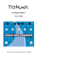
Overview
GAMMA provides interfaces between itself and the formats supported by several useful software
packages. This scheme is depicted in the following diagram.
GAMMA Supported I/O
Gnuplot
FrameMaker
Matlab
Γ
Felix
(FTNMR)
Bruker
UXNMR
NMRi
?
Figure 19-1 : Some of the programs with which GAMMA can easily interact. There are other
prgrams that also have been used with GAMMA, those that come to mind at the moment are SigmaPlot, Deltagraph and XMGR. These take ASCII input and need no special interface.
GAMMA has the ability to read and write data in the formats used by the programs in the figure.
Thus, GAMMA may be used to directly produce data in a format specific to any of these, or used
to swap data between the different programs. This allows the user to take advantage of any data
processing provided in these programs and any additional program which perform data conversions
on them.
Keep in mind that GAMMA itself has only rudimentary abilities for graphical display and signal
processing. It would be foolish to compete with professional and/or establish public domain programs that performs such tasks well. Furthermore, it is difficult to support all plotting and terminal
devices, there are plently of excellent software packages on the market which already perform this
duty. Our aim is simply to provide a means of reading and writing data files in the formats utilized
Scott Smith
Copyright S.A. Smith
May 22, 1998
GAMMA
Users Manual
Plotting
Plotting Figures
30
4.2
by such programs. A nice consequence of supporting multiple formats is that GAMMA may also
be used to perform format conversions.
GAMMA I/O Methodology
Matlab
Row Vector
Felix
(FTNMR)
class row_vec
Γ
FrameMaker
Simulation
Result(s)
Matrix
class matrix
Coordinate Vector
class coord_vec
Data To Be Plotted is Contained
In One Of These GAMMA Types
Gnuplot
Bruker
UXNMR
NMRi
Figure 19-2 : Some of the programs with which GAMMA can easily interact.
We should mention that there are currently NO direct plots from GAMMA to the
screen, NOR direct output to any specialized printing and plotting devices. There
are many ways to do “indirect” plots so that your programs will interactively display,
print, and/or plot. These are just GAMMA programs which output their data into one or more
of the supported formats, then call the associated program(s) from within the GAMMA program,
having it perform the visual and/or hardcopy output. In particular, see the Gnuplot section for programs which plot to screen interactively.
Scott Smith
Copyright S.A. Smith
May 22, 1998
GAMMA
Users Manual
4.4
4.4.1
Plotting
Plotting Figures
31
4.2
Gnuplot
Description
One way to have your plots appear on the screen during the course of a GAMMA simulation is to
have your program output its data into a file that is compatible with the Gnuplot program and then
call Gnuplot from within your program while it is running. Alternatively you can use Gnuplot to
view results of GAMMA simulations after program completion.
Typically, the GAMMA program files a vector or matrix full of simulated data. Then one of the
numerous gnuplot functions provided in GAMMA is called with the vector or matrix as one of the
function arguments. The gnuplot function writes out the data to an external file in a format which
is readable with gnuplot. If the plot is desired to be viewed during program execution then another
call is made to the system, either using other GAMMA gnuplot functions or with explicit code. To
view the plot using gnuplot after program completion, gnuplot is started and the appropriate commands issued to read the file created by the GAMMA program.
4.4.2
1D - Plots
The simplest type of plot is a 1D-plot created from a data vector with the function GP_1D. Withthis function the horizontal axis is the point index of vector and the vertical axis contains the data
value.
This program demonstrates how to have a 1D plot sent interactively to the screen using gnuplot.
Note that in order for it to work, the system command “gnuplot” must be known to the user running
the program.
#include <gamma.h>
main ()
{
int N = 4096;
row_vector data(N);
double rval, ival;
for(int i=0; i<N; i++)
{
rval = cos(33.33*double(i)/double(N-1));
data.put(rval, i);
}
GP_1D("real.asc", data, 0);
GP_1Dplot("real.gnu", "real.asc");
cout << "\n\n";
}
// Include GAMMA itself
// We'll plot this many points
// Here's a vector of points
// More temporaries
// Now we'll fill up the vector
// putting a cosine into the
// real part
// Write real points to ASCII file
// This will plot points in "real.asc"
// Keep the screen nice
The call to the function GP_1D produces an ASCII file called “real.asc” that is usable by the Gn-
Scott Smith
Copyright S.A. Smith
May 22, 1998
GAMMA
Users Manual
Plotting
Plotting Figures
32
4.2
uplot program. It will contain the cosine function which was put into the row_vector “data”. The
call to the function GP_1Dplot will make a plot on the screen of the data in “real.asc” during program execution. It first makes an ASCII gnuplot “load file” called “real.gnu” then runs gnuplot using the commands in the load file.
The following figure is “roughly” the plot that appears on the screen when you run the program.
What I’ve done here is re-run gnuplot after program completion, plotted the “real.asc” file, then
output the plot into this document (using Gnuplots MIF output).
1
"real.asc"
0.8
0.6
0.4
0.2
0
-0.2
-0.4
-0.6
-0.8
-1
0
500
1000
1500
2000
2500
3000
3500
4000
4500
There are a couple of very nice Gnuplot features worth mentioning. First and foremost is that it is
a program in public domain. Not only does the user not have to pay for it, one has access to the
entire source code and it runs on almost all common computer architectures. Second, Gnuplot has
many different output formats. That means that you can get your figures in PostScript, MIF (as was
done here) for FrameMaker, LaTex, PBM, even GIF.
Scott Smith
Copyright S.A. Smith
May 22, 1998
GAMMA
Users Manual
4.5
33
4.2
FrameMaker
4.5.1
4.5.2
4.5.4
4.5.5
4.5.6
4.5.7
4.5.8
4.5.9
4.5.10
4.5.11
4.5.1
Plotting
Plotting Figures
Description
1D Plots
xy-Plane Plots
Scatter Plots
2D Contour Plots
2D Stack Plots
3D Sphere Plots
Histograms
Matrix Output
Matrix Plots
page 33
page 33
page 36
page 37
page 38
page 40
page 42
page 43
page 44
page 45
Description
GAMMA provides functions for generation of figures suitable for direct use in FrameMaker (see
http://www.frame.com). The GAMMA functions are handed data, typically a matrix or vector, and
produce disk files in MIF (Maker Interchange Format) format or in the MML (Maker Mathematical
Language) format. Plots or data structures are then seen by simply opening the file with
FrameMaker. Such output may then be graphically manipulated and/or incorporated as part of a
document and data such a matrices placed into FrameMaker equations. Plots produced in this manner can be printed on a laserprinter in PostScript, colorized to make transparencies, converted into
HTML, etc.
One important point to realize is that these FrameMaker files are not changeable into other formats
with any GAMMA based code. If your data is valuable, and you wish to use it again in GAMMA,
it should be stored to disk in one of the other formats so that GAMMA can retreive and manipulate
it once again. There are some FrameMaker and public domain programs which can convert
FrameMaker files to other formats, but they must be obtained independently from GAMMA.
To see all specifics regarding these functions look in the GAMMA FrameMaker Documentation.
4.5.2
1D Plots
The simplest type of plot is a 1D-plot created from a data vector with the function FM_1D. Withthis function the horizontal axis is the point index of vector and the vertical axis contains the data
value. An example would be the simulated NMR spectrum shown below.
Scott Smith
Copyright S.A. Smith
May 22, 1998
GAMMA
Users Manual
Plotting
Plotting Figures
34
4.2
Ninety Ideal Pulse On A 4 Spin Proton System.
Have your GAMMA program fill up a row vector with the simulated data points you wish to plot.
Then make a function call to FM_1D with the row vector and an output file name given as arguments. The output file can be read by FrameMaker. Please note that GAMMA takes no time to
make “pretty” output, you can do the cosmetic work within FrameMaker!
Here is a simple example:
#include <gamma.h>
main ()
{
row_vector vx(101);
double x, y;
for(int i=0; i<101; i++)
{
x = double(i-50);
y = x*x*x/125000;
x = x*x/2500;
vx.put(complex(x,y),i);
}
FM_1D(“FM.mif”,vx,10,5, -50, 50, 1);
}
// 1-dim. data block (or use row_vector)
// Fill up data block
// cubical parabolic in imaginaries
// parabolic into reals
// output FM.mif with both plots
When compiled and run it will produce a file called FM.mif. When that file is subsequently read
by FrameMaker the following plots will appear. The one on the left has been left (except for resizing) as GAMMA produced, the one on the right has been cosmetically enhanced just to show what
you can do to the plot in FrameMaker.
Scott Smith
Copyright S.A. Smith
May 22, 1998
GAMMA
Users Manual
Plotting
Plotting Figures
1
0.8
0.6
0.4
0.2
0
-40
4.5.3
-20
0
20
40
35
4.2
1
0.5
0
-0.5
-1
Wow! I can do anything
I want to with this plot now!
-40
-20
0
20
40
Multiple 1D - Plots
You can easily output several plots into the same graph by using the function FM_1Dm. Instead of
providing a single vector to the function the user just provides an array of vectors.
Dipolar Longitudinal Relaxation Times versus Correlation Time
13C
by 19F
by 1H
13C by 3H
19F
relaxed by 13C
3H relaxed by 13C
13C relaxed by 13 C
6
13C
13C
by 13C
4
ln T1
1H
by 19F
19
F by 1H
2
3
H by 19F
19F by 3H
19F
by 19F
by 1H
3
H by 3H
1H
0
-12
1
H relaxed by 3H
3H relaxed by 1H
-11
-10
log τ
-9
-8
Figure 19-3 Dipolar longitudinal relaxation times for several spin pairs versus correlation time. The
Scott Smith
Copyright S.A. Smith
May 22, 1998
GAMMA
Users Manual
Plotting
Plotting Figures
36
4.2
distance between the spins was kept at 2A and the field strength set to 500 MHz.
The above plot was made with a simple GAMMA program using the FM_1Dm program (see
GAMMA DIPOLAR RELAXATION DOCUMENTATION).
4.5.4
xy-Plane Plots
Plots in the xy-plane can be produced with the FrameMaker function FM_xyPlot. Unlike the function FM_1D, this function need not have the horizontal coordinate always increasing. The plot below is a typical example. It has been annoted and resized in FrameMaker after creatation with
GAMMA.
rf-Field Offset Effects
0.6
Increasing
Offset
MDis. 0.4
M0
0.2
0
-0.2
0
0.2
0.4
0.6
0.8
1
MAbs.
M0
Have your GAMMA program fill up a row vector with the simulated data points you wish to plot.
Then make a function call to FM_xyPlot with the row vector and an output file name given as arguments. The output file can be read by FrameMaker. Please note that GAMMA takes no time to
make “pretty” output, you can do the cosmetic work within FrameMaker!.
Here is a simple example:
#include <gamma.h>
main ()
{
row_vector vx(360);
double x,y,theta;
for(int i=0; i<360; i++)
{
theta = i*2.0*PI/360.0;
x = cos(theta);
y = sin(theta);
Scott Smith
// create a data block
// declare needed variables
// loop through 360 degrees
// fill up block with Astroid
// also called a Hypercycloid of four cusps
// x = a*[cos(theta)]**3, here a = 1
// y = a*[sin(theta)]**3, here a = 1
Copyright S.A. Smith
May 22, 1998
GAMMA
Users Manual
Plotting
Plotting Figures
x = x*x*x;
y = y*y*y;
vx.put(complex(x,y), (i);
}
FM_xyPlot(“astroid.mif”, BLK);
}
37
4.2
// output FrameMaker .mif plot file
When compiled and run it will produce a file called astroid.mif. When that file is subsequently read
by FrameMaker the following plot on the left will appear. The one on the right is just a copy that
I’ve jerked with within FrameMaker.
1
1
0.5
.5
0
0
-0.5
-.5
-1
-1
4.5.5
-0.5
0
0.5
1
-1
β
α
❁❂❃
-1
-0.5
0
0.5
1
Scatter Plots
Scatter plots can be generated for FrameMaker with the function FM_scatter. These are similar to
plots produced with the function FM_xyPlot except that the plots are not connected and can be individually plotted with symbols or characters.
3
2
1
0
-2
0
2
4
6
8
I forget why I even wrote this function now. Perhaps I used it to have my point plotted on top of a
theoretical curve by blending a graphic like the one above with another one with a continuous line.
Here’s the code for the one above.
Scott Smith
Copyright S.A. Smith
May 22, 1998
GAMMA
Users Manual
Plotting
Plotting Figures
#include <gamma.h>
main ()
{
block_1D BLK(50);
double x,y,theta;
double a,b;
for(int i=0; i<50; i++)
{
a = 1;
b = 2;
theta = -PI + i*(4.0*PI/49.0);
x = a*theta - b*sin(theta);
y = a - b*cos(theta);
BLK(i) = complex(x,y);
}
FM_scatter(“FM.mif”, BLK, 0, .1, 14, 5);
}
38
4.2
// create a data block
// declare needed variables
// declare needed variables
// loop through 50 points
// fill up block with Prolate Cycloid
// angles span -pi to 3pi
// x = a(theta) - b*sin(theta), here a=1, b=2
// y = a - b*cos(theta)
// output FrameMaker .mif plot file
You can set the symbol type to use in the figure either in the function call or afterwards in
FrameMaker..
4.5.6
2D Contour Plots
2D contour plots are produced for FrameMaker with function FM_contour. Each contour is an individual graphic object which can be manipulated. For example, the negative contours can selectively changed to dashed lines. Overall plot height & width can be set within FrameMaker.
Scott Smith
Copyright S.A. Smith
May 22, 1998
GAMMA
Users Manual
Plotting
Plotting Figures
39
4.2
1
0.8
0.6
0.4
0.2
0
-0.2
0.8
0.6
0.4
0.2
0
The example plot has be altered within FrameMaker and the 1D-plots added. Thsi program made it.
#include <gamma.h>
main()
{
matrix mx(101, 101);
row_vector BLK1(101), BLK2(101);
BLK1 = sinc(101, 50, 10);
BLK2 = sin_square(101, 50);
for(int i=0; i<101; i++)
for(int j=0; j<101; j++)
mx(i,j) = BLK1(i) * BLK2(j);
FM_contour(“contour.mif”,mx,.05,10,.05);
}
// create a 101x101 matrix for data
// create two 1D-data blocks of length 101
// use provided window sinc function
// use provided window sin squared function
// loop through and fill up the matrix
//create file FM contour file - contour.mif
You can just use the computer to remove your T1 noise now! Read your spectrum (F1xF2) into a
GAMMA matrix, output the contour plot into FrameMaker, Edit As You Wish (removing artifacts
you don’t want anyone to see, no more white out.......), Print to A Tranparency. Too Easy.
Scott Smith
Copyright S.A. Smith
May 22, 1998
GAMMA
Users Manual
4.5.7
Plotting
Plotting Figures
40
4.2
2D Stack Plots
Two dimensional stack plots are produced for FrameMaker with the function FM_stack. The function is called with a GAMMA matrix as an input argument.
The function automatically used a hidden line algorithm (which can be removed in FrameMaker)
and the user may set the skew. Each plotted row is an individual graphic object which can be manipulated. For example, a particular slice in the plot below was selectively shaded. The overall plot
height and width can be altered as well within FrameMaker.
Here is a simple program, the one that produced the plot above.
#include <gamma.h>
main()
{
matrix mx(101, 101);
block_1D vx(100);
vx = sinc(101, 50, 10);
for(int i=0; i<101; i++)
for(int j=0; j<101; j++)
mx(i,j) = vx(i) * vx(j);
FM_stack(“stack.mif”, mx, 0.02, 0.02, 1);
}
// create a 101x101 matrix for data
// create a 1D-data block of length 101
// use provided window sinc function
// loop through and fill up the matrix
// output the FrameMaker .mif plot file
The output file, stack.mif, can be read into FrameMaker and below are some of the manipulations
that can be subsequently performed.
Scott Smith
Copyright S.A. Smith
May 22, 1998
GAMMA
Users Manual
Plotting
Plotting Figures
41
4.2
Original Plot
Specific Line Highlighted
Positive, in plane, & negative
Specific Line Isolated
Rescaled
Original Plot
Hidden Lines now Visible
Scott Smith
Rotated
Copyright S.A. Smith
May 22, 1998
GAMMA
Users Manual
4.5.8
Plotting
Plotting Figures
42
4.2
3D Sphere Plots
Three dimensional sphere plots are produced for FrameMaker with the function FM_sphere. This
is real handy for making 3-dimensional plots of trajectories, for example
Unlike other FM functions, this function takes a vector of coordinates (class coord_vec) which are
assumed to be in Cartesian space. There function allows the user to orient the sphere and to plot
either with vectors from the origin to the points, with a line connecting points, or just with the
points plotted individually. As with all other FM function, the user can fully manipulate the plot
within FrameMaker after it is output by GAMMA. Here is a simple example program.
#include <gamma.h>
main ()
{
coord_vec data1(500);
coord_vec data2(500);
double xx, yy, zz;
double theta;
for(int i=0; i<500; i++)
{
theta = i*6.0*PI/499.0;
xx = 3.0*cos(theta);
yy = 3.0*sin(theta);
zz = 3.0 - (6.*i/499.);
data1.put(xx, yy, zz, i);
}
data2 = data1.rotate(90,90,0);
Scott Smith
// Declare a 500 point coordinate vector
// A second coordinate vector
// Declare needed variables
// Declare an angle variable
// Fill data1 with a spiral
// Set 2nd coordinate vector to rotated data1
Copyright S.A. Smith
May 22, 1998
GAMMA
Users Manual
Plotting
Plotting Figures
FM_sphere(“FM_sph2a.mif”, data1,0);
FM_sphere(“FM_sph2b.mif”, data2,1);
}
43
4.2
// Output FrameMaker file FM_sph2a.mif
// Output FrameMaker file FM_sph2b.mif
The program will produce two plot files, FM_sph2a.mif and FM_sp[h2b.mif which are shown below. I marked the points in red within FrameMaker after the fact.
4.5.9
Histograms
Histogram plots can be generated for FrameMaker with the function FM_histogram.
1
0.8
0.6
0.4
0.2
0
10
20
30
40
50
Here is a little program that illustrates how to make FrameMaker histograms in a GAMMA program.
#include <gamma.h>
main ()
{
row_vector vx(51);
row_vector vx1 = Gaussian(51, 25, 3);
Scott Smith
// create a data block
// fill up data with Gaussian
Copyright S.A. Smith
May 22, 1998
GAMMA
Users Manual
Plotting
Plotting Figures
for(int i=0; i<51; i++)
vx(i) = complex(i, Re(vx1(i)));
FM_histogram(“FM.mif”, vx, bins);
}
44
4.2
// output FrameMaker .mif plot file
I colored some of the boxes in FrameMaker after reading the file FM.mif into that program. Perhaps one of the nicer uses of this function is to make cool plots of your pulse shape functions. Once
again we see the typical scheme for getting plotted output from GAMMA. We do something to fill
some array, in this case a row vector, with some simulated data we wish to plot. Then one (or more)
of the plot functions is called with the array as one of the arguments.
4.5.10 Matrix Output
Matrices can be output for FrameMaker equations with the function FM_matrix. For example, the
following double commutation superoperators given below were incorporated directly from GAMMA into this document.
D
D
D
[ T 2, 1 ( kl ), [ T 2, –1 ( kl ), ] ]
-2
0
0
0
0
1
1
1 0
-----16 0
1
1
0
0
0
0
0
0
-3
-1
0
0
0
0
-1
0
0
0
-1
0
0
0
0
0
-1
-3
0
0
0
0
-1
0
0
0
-1
0
0
0
0
0
0
0
-4
0
0
0
0
0
0
0
0
0
0
0
0
0
0
0
0
-1
0
0
0
-1
0
0
0
0
-1
-1
0
1
0
0
0
0
-2
-1
0
0
-1
0
0
0
0
0
1
1
0
0
0
0
-1
-2
0
0
0
-1
0
0
0
0
1
0
-1
-1
0
0
0
0
-3
0
0
0
-1
0
0
0
0
0
0
0
0
-1
0
0
0
-1
0
0
0
0
-1
-1
0
1
0
0
0
0
-1
0
0
0
-2
-1
0
0
0
0
1
1
0
0
0
0
0
-1
0
0
-1
-2
0
0
0
0
1
D
[ T 2, –1 ( kl ), [ T 2, 1 ( kl ), ] ]
0
-1
-1
0
0
0
0
-1
0
0
0
-3
0
0
0
0
0
0
0
0
0
0
0
0
0
0
0
0
0
0
0
0
0
0
0
0
-1
0
0
0
-1
0
0
0
0
-1
-1
0
0
0
0
0
-1
0
0
0
-1
0
0
0
0
-1
-1
0
0
0
0
0
0
1
1
0
0
1
1
0
0
0
0
-2
-2
0
0
0
0
1
1
1 0
-----16 0
1
1
0
0
0
0
0
0
-1
-1
0
0
0
0
-1
0
0
0
-1
0
0
0
0
0
-1
-1
0
0
0
0
-1
0
0
0
-1
0
0
0
0
0
0
0
0
0
0
0
0
0
0
0
0
0
0
0
0
0
0
0
0
-3
0
0
0
-1
0
0
0
0
-1
-1
0
1
0
0
0
0
-2
-1
0
0
-1
0
0
0
0
0
1
1
0
0
0
0
-1
-2
0
0
0
-1
0
0
0
0
1
0
-1
-1
0
0
0
0
-1
0
0
0
-1
0
0
0
0
0
0
0
0
-1
0
0
0
-3
0
0
0
0
-1
-1
0
1
0
0
0
0
-1
0
0
0
-2
-1
0
0
0
0
1
1
0
0
0
0
0
-1
0
0
-1
-2
0
0
0
0
1
0
-1
-1
0
0
0
0
-1
0
0
0
-1
0
0
0
0
0
0
0
0
0
0
0
0
0
0
0
0
-4
0
0
0
0
0
0
0
-1
0
0
0
-1
0
0
0
0
-3
-1
0
0
0
0
0
-1
0
0
0
-1
0
0
0
0
-1
-3
0
0
0
0
0
0
1
1
0
0
1
1
0
0
0
0
-2
Here is a simple example of how this is done.
#include <gamma.h>
main ()
{
matrix mx(3, 4, complex0);
for(int i=0; i<mx.rows(); i++)
mx.put(6, i, 0);
for(int j=0; j<mx.cols(); j++)
mx.put(complexi, 0,j);
mx.put(complex(2,3), 1,2);
Scott Smith
// Make a 3x4 array, filled with zero
//Put 6’s in the first column
// Put i’s in the first row
// Set <3|mx|4> to 2+3i
Copyright S.A. Smith
May 22, 1998
GAMMA
Users Manual
Plotting
Plotting Figures
FM_Matrix(“FM.mmf”, mx);
}
45
4.2
// Output FrameMaker .mmf file
Here is the output from the program, the contents of file FM.mmf read by FrameMaker.
1⋅i 1⋅i
1⋅i
1⋅i
6 0 (2 + 3 ⋅ i) 0
6 0
0
0
4.5.11 Matrix Plots
While the previous function is great for putting matrices into your documents (remember cout <<
mx will print any array to the screen), often the arrays in GAMMA programs are just too darn big
to look at. Every once in a while we just need a graphical representation of which elements are nonzero rather than what the actual elements are. For that purpose you can use the function
FM_Mat_Plot.
For an example, we’ll just reuse the previous program but with the FM_Mat_Plot function instead
of FM_Matrix.
#include <gamma.h>
main ()
{
matrix mx(3, 4, complex0);
for(int i=0; i<mx.rows(); i++)
mx.put(6, i, 0);
for(int j=0; j<mx.cols(); j++)
mx.put(complexi, 0,j);
mx.put(complex(2,3), 1,2);
FM_Mat_Plot(“FM.mif”, mx);
}
// Make a 3x4 array, filled with zero
//Put 6’s in the first column
// Put i’s in the first row
// Set <3|mx|4> to 2+3i
// Output FrameMaker .mmf file
Here is the output from the program, the contents of file FM.mif read by FrameMaker.
Scott Smith
Copyright S.A. Smith
May 22, 1998
GAMMA
Users Manual
Plotting
Plotting Figures
46
4.2
Those familiar with FrameMaker should not that the result of this function is a graphical object
whereas the result of the previous function goes into an equation.
Scott Smith
Copyright S.A. Smith
May 22, 1998
GAMMA
Users Manual
4.6
4.6.1
Plotting
Plotting Figures
47
4.2
Felix
Description
GAMMA has some knowledge of the Felix NMR processing program. It contains a class for performing I/O to and from Felix files (and to the older FTNMR).
Scott Smith
Copyright S.A. Smith
May 22, 1998
GAMMA
NMR Examples
5
NMR Simulations
NMR Simulation Sections
48
5.1
NMR Simulations
If you have been following diligently through this book you now know how to build C++ programs
and GAMMA programs. You also know how to weild the GAMMA supplied data types as well as
the wide variety of functions supplied. We combine all of that knowledge in this section and embark on some NMR simulations.
5.1
NMR Simulation Sections
Single Pulse, Acquisition Simulations
3.4.1
Description
3.4.2
1D Plots
FrameMaker - Output to FrameMaker (MIF)
3.5.1
Description
page 48
page 28
page 28
page 30
page 30
5.2
NMR Simulation Figures
5.3
Single Pulse, Acquisition Simulations
The simplest NMR experiment one can simulate is that of a single pulse experiment. A pulse is
applied to the system with subsequent FID acquisition. The pulse sequence is depicted in the following diagram.
Simple Pulse Acquisition Sequence
Pulse
Acquire
Even with this simple experiment there are several tradeoffs between computational simplicty1
1. Do not confuse computational ease with programming ease. The intent of GAMMA is to make complicated simulations relatively easy to produce. In many instances the more computationally intensive simulations are produced from GAMMA programs which are not significantly more complex.
Tilo Levante, Scott Smith
May 22, 1998
GAMMA
NMR Examples
NMR Simulations
Single Pulse, Acquisition Simulations
49
5.3
and simulation accuracy which one may wish to consider. Below is again the pulse sequence diagram with GAMMA provided simulation possibilities listed for each of the two steps.
Single Pulse Experiment Simulation Possibilities
Step 1
Pulse
Step 2
Acquisition
A. “Ideal”
B. Real, No Relaxation
I. No Relaxation
C. Real, Relaxation
D. Shaped, No Relaxation II. Relaxation
E. Shaped, Relaxation
For the application of any pulse in GAMMA, users may opt to apply what we call an “ideal” pulse.
An ideal pulse affects all spins of a particular isotope equally and occurs instantaneously. This
would be suitable when one is not particularly concerned with the effects of relaxation, pulse
shape, or pulse length (phasing problems). Being the easiest to implement computationally, it
might also be used when one desires the most rapid simulation.
When the pulse itself is of concern one may apply either a square pulse of finite length, which we
call a “real” pulse, or an individually tailored shaped pulse. Although these take use more computer time, the simulation becomes more realistic. Real pulses have user specified lengths and
strengths so may be used for frequency selection, spin locking, etc The same is true for shaped
pulses but then users have the additional ability to specify the pulse waveform in the time domain.
Another level of complexity involves the treatment of relaxation, both while the rf-field is applied
and during the FID acquisition. This is not applicable to ideal pulses as they are infinitely short.
During the application of real and shaped pulse application and during acquisition, steps which
are of finite length, appreciable relaxation may occur. This of course depends upon input relaxation strengths and step times. Inclusion of relaxation effects will always increase program execution time and should only be used when of true concern or for comparison with analogous
experiments without relaxation. Normally, it is the relaxtion during the FID acquisition that is most
important as this contributes the most to spectral linewidths.
We shall NOT cover all of these aspects in these documents. See one of the GAMMA Examples
DOCUMENTATION Books. Instead we will do just a couple of such simulations and try and cover the fundamental aspects of these calculations.
Tilo Levante, Scott Smith
May 22, 1998
GAMMA
NMR Examples
NMR Simulations
Ideal 90 Pulse - 4,8,(N) Homonuclear Spin Systems
50
5.4
I most often use FrameMaker output of the simulated spectra so that they may be incorporated directly into this document. You don’t have to. Just go back to the “Plotting” chapter, find
the appropriate command(s) to relace the “FM” output function that will output the spectra in the
format you can deal with. On occasion I’ll add in a couple of output formats.
5.4
Ideal 90 Pulse - 4,8,(N) Homonuclear Spin Systems
Since you’ve gone through this user manual and are now a seasoned GAMMA programmer, we’ll
work on a general level in our programs (even if we use simple mathematical models). The figure
below is the pulse sequence we want to simulation, the “sigmas” are density operators that define
the state of the spin system trough the pulse sequence.
π/2y
σ0
Acquire
σ
σ(t2)
To keep the program general (and simplify the code) we’ll read in our spin system - that which defines the sample in the spectrometer - from an external ASCII file. You’ll see this treatment time
and time again because reading in the system is highly desirable when working with large spin systems, with using the same system repeatedly in different programs, or when running the same program with differing spin systems. At the same time, the code presented will be set to run
interactively, taking parameters (the spin system filename, dwell time, number of acquisition
points) either from the command line or interactively by query to the user. For this example, if the
spin system filename is not given as input the program will ask for it then wait for the filename to
be supplied. We will test the program on two different test systems, both forms of parameter input
will be demonstrated.
5.4.1 Program
#include <gamma.h>
main (int argc, char* argv[])
{
String filename;
double dt;
Tilo Levante, Scott Smith
// Read in Parameters
// Name of spin system file
// Dwell time for acquisition
May 22, 1998
GAMMA
NMR Examples
NMR Simulations
Ideal 90 Pulse - 4,8,(N) Homonuclear Spin Systems
51
5.4
int t2pts;
// Number of points in FID
query_parameter(argc, argv,
// Get or ask for filename (#1)
1, “\nSpin system filename? “, filename);
query_parameter(argc, argv,
// Get or ask for dwell time (#2)
2, “\nDwell time? “, dt);
query_parameter(argc, argv,
// Get or ask for block size (#3)
3, “\nNumber of points? “, t2pts);
spin_system sys;
// Declare spin system sys
sys.read(filename);
// Read system from filename
// Set Variables
block_1D data(t2pts);
// Storage for the FID/Spectrum
gen_op sigma = sigma_eq(sys);
// Set density matrix equilibrim
gen_op H = Hcs(sys) + HJ(sys)
// Set the Hamiltonian
gen_op detect = Fm(sys);
// Set detection operator to F// Pulse Sequence, Data Workup
sigma = Iypuls(sys, sigma, 90);
// Apply a (PI/2)y pulse
FID(sigma,detect,H,dt,t2pts,data);
// Calculate the FID after the pulse
NMRi(“One_pulse.2.dat”,data);
// Write data in NMRi format
exponential_multiply(data, -8);
// Apodize the FID
data = FFT (data);
// Fourier transform the FID
FM_1D (“One_pulse.2.mif”,
// Write spectrum to FrameMaker file
data, 14, 5,-0.5/dt, 0.5/dt);
// with frames of the size 5*14 cm
}
5.4.2 Discussion
Read in Parameters: Note that in the program start, main, there are now two arguments, argc
and argv. This is a means by which programs in C and C++ can take parameters supplied directly
from the command line at run-time1. Three parameters are asked for using GAMMA’s function
“query_parameter”: the spin system filename, the dwell time, and the number of points in the acquisition. When the program is run, values for these can be given directly or (if not given) the
program will automatically ask for them. If the values are given, the program will not ask for them.
The spin system is then read in from the file.
Set Variables: The first line here creates a data block of the proper size. The density matrix is
declared and set to equilibrium. Another general operator, H, is specified and initialized to the liquid NMR Hamiltonian with strong (homonuclear) coupling. The detection operator is declared and
set to F-.
1. FORTRAN programmers may find this unfamiliar territory. In C and C++, the program itself is structured
as any other routine: it has a name (main), its code is encased in brackets ({}), and it may take arguments.
Tilo Levante, Scott Smith
May 22, 1998
GAMMA
NMR Examples
NMR Simulations
Ideal 90 Pulse - 4,8,(N) Homonuclear Spin Systems
52
5.4
Pulse Sequence, Data Workup: The pulse sequence is very short; two steps and two pro-
gram lines. The first step makes use of the function Iypuls which takes σ0, the equilibrium density
matrix and applies a 90 pulse along the y-axis to it. The resulting density matrix is set equal to
sigma. The next function, FID, propagates sigma under the active Hamiltonian H while filling up
the data block. The detector, the number of points, and the dwell time are also parameters used as
arguments for this function. Following this, the FID is sent out to a file One_pulse.2.dat in NMR1
compatible format. The FID is then internally manipulated by an exponential multiplication, Fourier transformation, and finally an output to the file One_pulse.2.mif in FrameMaker format. I left
in a line to output the unprocessed FID to an NMRi compatible file for those who use that software.
5.4.3 Example Data - 4 Spin System
The first spin system file One_pulse.2.sys contains:
SysName (2) : antamanide - Name of the Spin System
NSpins (0) : 4
- Number of Spins in the System
Iso(0) (2) : 1H
- Spin Isotope Type
Iso(1) (2) : 1H
- Spin Isotope Type
Iso(2) (2) : 1H
- Spin Isotope Type
Iso(3) (2) : 1H
- Spin Isotope Type
v(0)
(1) : 200.0 - Chemical Shifts in Hz
v(1)
(1) : 40.0 - Chemical Shifts in Hz
v(2)
(1) : -10.0 - Chemical Shifts in Hz
v(3)
(1) :-200.0 - Chemical Shifts in Hz
J(0,1) (1) : 5.0 - Coupling Constants in Hz
J(0,2) (1) : 0.0 - Coupling Constants in Hz
J(0,3) (1) : 0.0 - Coupling Constants in Hz
J(1,2) (1) : 10.0 - Coupling Constants in Hz
J(1,3) (1) : 0.0 - Coupling Constants in Hz
J(2,3) (1) : 8.0 - Coupling Constants in Hz
Omega (1) : 400 - Spectrometer Frequency in MHz (1H based)
5.4.4 Results - 4 Spin System
The program was compiled with the command
gamma One_pulse.2.cc -o One_pulse.2
This takes the gamma library and links to the program One_pulse.2.cc during compilation. The o option specifies the name of the final executable program, in this instance called One_pulse.2.
Had the -o option not been used (-o One_pulse.2 left out) the executable program is automatically
Tilo Levante, Scott Smith
May 22, 1998
GAMMA
NMR Examples
NMR Simulations
Ideal 90 Pulse - 4,8,(N) Homonuclear Spin Systems
53
5.4
given the name a.out.
The compiled program was called with
One_pulse.2 One_pulse.2.sys 0.002 1024
Since we have given the executable the name One_pulse.2 it is run by entering that name. The program, having been given all needed parameters, will run to completion without asking questions to
the user. The program writes two files, one data file with the FID in the format of the NMRi program and the other (processed) spectrum file in FrameMaker format, the later is below.
250
200
150
100
50
-200
-100
0
100
200
An alternative way of running the program is to let it prompt the user for needed information. The
following is a second way of achieving the same results.
One_pulse.2
Spin system filename? One_pulse.2.sys
Dwell time? 0.002
Number of points? 1024
Since the parameters were not supplied on the command line which executed the program
One_pulse.2.sys, the program responds by asking the user to supply them. The results are of course
identical to that as when the parameters are given on the command line.
5.4.5 Example Data - 8 Spin System
The second spin system file One_pulse.2a.sys contains
SysName (2)
NSpins (0)
Iso(0) (2)
Iso(1) (2)
Iso(2) (2)
Iso(3) (2)
Iso(4) (2)
:
:
:
:
:
:
:
Tilo Levante, Scott Smith
galact - Name of the Spin System (galactose)
8
- Number of Spins in the System
1H
- Spin Isotope Type
1H
- Spin Isotope Type
1H
- Spin Isotope Type
1H
- Spin Isotope Type
1H
- Spin Isotope Type
May 22, 1998
GAMMA
NMR Examples
NMR Simulations
One Ideal Pulse - Homonuclear Spin System
Iso(5) (2)
Iso(6) (2)
Iso(7) (2)
PPM(0) (1)
PPM(1) (1)
PPM(2) (1)
PPM(3) (1)
PPM(4) (1)
PPM(5) (1)
PPM(6) (1)
PPM(7) (1)
J(0,1) (1)
J(1,2) (1)
J(2,3) (1)
J(3,4) (1)
J(4,5) (1)
J(5,6) (1)
J(6,7) (1)
Omega (1)
:
:
:
:
:
:
:
:
:
:
:
:
:
:
:
:
:
:
:
1H
1H
1H
4.27
3.47
3.6
3.89
3.63
3.76
3.71
3.54
7.8
8.2
3.7
4.0
10.5
10.5
15
400
-
54
5.5
Spin Isotope Type
Spin Isotope Type
Spin Isotope Type
Chemical Shifts in PPM
Chemical Shifts in PPM
Chemical Shifts in PPM
Chemical Shifts in PPM
Chemical Shifts in PPM
Chemical Shifts in PPM
Chemical Shifts in PPM
Chemical Shifts in PPM
Coupling Constants in Hz
Coupling Constants in Hz
Coupling Constants in Hz
Coupling Constants in Hz
Coupling Constants in Hz
Coupling Constants in Hz
Coupling Constants in Hz
Spectrometer Frequency in MHz (1H based)
5.4.6 Results - 8 Spin System
The second example was done with: One_pulse.2.One_pulse.2a.sys 0.0025 1024
6000
5000
4000
3000
2000
1000
-200
5.5
-100
0
100
One Ideal Pulse - Homonuclear Spin System
For the next example of a single pulse experiment simulation we present a more complicated program which will work on any input spin system. The pulse sequence is again shown below with
density matrices labeled to coincide with the program code.
Tilo Levante, Scott Smith
May 22, 1998
GAMMA
NMR Examples
NMR Simulations
One Ideal Pulse - Homonuclear Spin System
π/2y
σ0
55
5.5
Acquire
σ
σ(t2)
The spin system, acquisition size, isotope to be detected, and output format at will all be specified
by the user interactively. Following this, the spin system shifts will be offset to the center of the
spectrum so the simulation occurs in an optimal rotating frame. All spectral parameters such as the
spectral width and dwell time will be determined automatically. The equilibrium density matrix,
σ0, can be generated directly from the specified spin system. This density matrix is then treated
by a 90 degree pulse along the y-axis and propagated in time (without relaxation effects) while the
FID is computed. The detection operator, necessary for determining the FID, will be set to F- for
the entire spin system. The is equivalent to a operator which samples by xy-magnetization. Use of
F- as the detection operator , in combination with a pulse along the y-axis produces a properly
phased spectrum.
Again we must mention that the FID does not decay, as shown in the pulse sequence diagram. For
that relaxation effects must be included or the FID apodized. Since we here ignore relaxation effects it is assumed the user will apply some apodization in the spectral workup prior to Fourier
transformation (done automatically for FrameMaker output). Also, the code is written to be clear
and concise. Although efficient, it is not the most computationally efficient.
5.5.1 Program
#include <gamma.h>
main (int argc, char* argv[])
{
cout << “\n\n\t\t\tGAMMA 1D NMR Simulation Program\n\n”;
//
Read in Parameters
String filename;
query_parameter(argc, argv,
1, “\n\tSpin system filename? “
// Name of spin system file
// Get filename from command
// line or ask for them
, filename);
spin_system sys;
Tilo Levante, Scott Smith
// Declare spin system sys
May 22, 1998
GAMMA
NMR Examples
NMR Simulations
One Ideal Pulse - Homonuclear Spin System
sys.read(filename);
int t2pts;
query_parameter(argc, argv,
2, “\n\tNumber of acquisition points? “, t2pts);
char J;
query_parameter(argc, argv,
3, “\n\tStrong or Weak Coupling (s/w)? “ , J);
56
5.5
// Read system from filename
// Number of points in FID
// Get number of points
// Get number of points
// Determine the Isotope Detection Type
int isoset = 0;
String Isotype = sys.symbol(0);
// Get isotope type of first spin
if(sys.heteronuclear())
// Check if system is heteronuclear
{
isoset--;
while(isoset < 0)
{
cout << “\n\tWhich Isotope Type? “;
cin >> Isotype;
for(int k=0; k<sys.spins(); k++)
if(Isotype == sys.symbol(k))
{
isoset = k;
break;
}
if(isoset < 0)
cout << “\n\tSystem Contains No Spin of That Type!”;
}
}
// Set Up Spectral Parameters
double offset = sys.center(isoset);
sys.offsetShifts(offset, isoset);
double NyqF = sys.Nyquist();
double dt = 1.0/(2.0*NyqF);
double sw = 2.0*NyqF;
//
Tilo Levante, Scott Smith
// Find the center of the system
// Offset the rotating frame
// Approximate Nyquist frequency
// Dwell time, quadrature detection
// Total Spectal width +/- Nyquist
Set Variables
May 22, 1998
GAMMA
NMR Examples
NMR Simulations
One Ideal Pulse - Homonuclear Spin System
block_1D data(t2pts);
gen_op sigma = sigma_eq(sys);
gen_op H;
if(J == ‘w’)
H = Hcs(sys) + HJw(sys);
else
H = Hcs(sys) + HJwh(sys);
gen_op detect = Fm(sys, Isotype);
//
// Storage for the FID/Spectrum
// Set density matrix equilibrium
// Set the weak coupling Hamiltonian
// Set the strong coupling Hamiltonian
// Set detection operator to FPulse Sequence
sigma=Iypuls(sys,sigma,Isotype,90);
FID(sigma,detect,H,dt,t2pts,data);
//
57
5.5
// Apply an (PI/2)y pulse
// Calculate the FID after the pulse
Spectral Output Format & File Selection
int type = 0;
// Select an output format
while((type <=0) || (type > 4))
{
cout << “\n\tPlease Choose an Output Format”;
cout << “\n\n\t\t1. FrameMaker”;
cout << “\n\t\t2. Felix”;
cout << “\n\t\t3. NMRi”;
cout << “\n\t\t4. MatLab”;
cout << “\n\n\tOutput Type? “;
cin >> type;
cout << “\n”;
}
cout << “\n\tOutput File Name - Please Include any Extension? “;
if(type == 2)
{
cout << “\n\tFelix 1D Files Normally Use a .dat Extension”;
cout << “\n\t(Remember Felix reads only lower case names!) “;
}
cin >> filename;
//
Spectral Output
cout << “\n”;
switch(type)
Tilo Levante, Scott Smith
May 22, 1998
GAMMA
NMR Examples
NMR Simulations
One Ideal Pulse - Homonuclear Spin System
58
5.5
{
case 1:
// FrameMaker output
default:
double lf, rt;
double inPPM = 2;
lf = offset-(sw/2.0);
// Set plot limits in Hertz
rt = offset+(sw/2.0);
while(inPPM <0 || inPPM >1)
// Querie for Hertz or PPM axis
{
cout << “\n\n\tAxes in Hz(0) or PPM(1)? “;
cin >> inPPM;
cout << “\n”;
}
if(inPPM)
// For PPM adjust plot limits
{
lf = lf/sys.Omega();
rt = rt/sys.Omega();
}
exponential_multiply(data,-8);
// Apodize the FID
data = FFT(data);
// Fourier transform the FID
FM_1D(filename,data,14,5,lf,rt); // Write spectrum to a FrameMaker file
break;
case 2:
// Felix output
Felix(filename,data);
// Output FID in Felix format
cout << “\n\t\tParameters Needed for Felix Data Workup\n”;
cout << “\n\tTo set OMEGA
: sf “ << sys.Omega(isoset);
cout << “\n\tTo set spectral width: sw “ << 2*NyqF;
cout << “\n\tTo set offset (no zf): ref “ << t2pts/2 << “ “ << offset;
cout << “\n\tTo set axis in Hertz : ax 2” << “\n\n”;
break;
case 3:
NMRi(filename,data);
// Output FID in NMRi format
break;
case 4:
MATLAB(filename,”spectrum”,data);
// Output FID in MatLab format
cout << “\n\t\tMATLAB Spectrum is Internally Named: spectrum”;
break;
cout << “\n”;
}
Tilo Levante, Scott Smith
May 22, 1998
GAMMA
NMR Examples
NMR Simulations
One Ideal Pulse - Homonuclear Spin System
59
5.5
}
5.5.2 Discussion
Read in Parameters: Following the output of the program description, an arbitrary spin system is read in from an external file specified. Afterwards the number of points in the FID is interactively set. Because it is useful to examine the weak coupling case, the user is then allowed to
specify weak or strong coupling.
Determine the Isotope Detected: A check is made to see if the input spin system is homonuclear or heteronuclear. If heteronuclear, the user must choose the isotope type to be detected.
Set Up Spectral Parameters: Here, all chemical shifts (for spins of the isotope type being
detected) may be altered so as to be referenced to an optimal rotating frame. Following this, a
Nyquist frequency is chosen and both the dwell time and spectral width set.
Set Variables: A 1D data block is declared to hold the simulated FID. A general operator is
declared and set to the equilibrium density matrix. Another general operator is declared and set to
be either the strong or weak coupling isotropic Hamiltonian. Finally, a general operator is declared
and set to hold the detection operator.
Pulse Sequence: The pulse sequence is very short; a two step sequence is performed with two
program lines. The first step makes use of the function Iypuls which takes σ0, the equilibrium density matrix and applies a 90 pulse along the y-axis to it. The resulting density matrix is set equal
to sigma. The next function, FID, propagates sigma with the Hamiltonian H while filling up the
data block. The detector, the number of points, and the dwell time are also parameters used as arguments for this function.
Spectral Output Format & File Selection: The user is prompted to specify an output type.
Currently four formats are allowed.
Spectral Output: In this section the simulated FID is written to an output file. For FrameMaker
output, the FID is apodized and Fourier Transformed before output since that program has not FFT
capabilities. Because Felix currently has problems accepting data into its parameter block, the parameters needed to reference the spectrum are output if this format is specified. For MATLAB output, there may be several “matrices” stored in each .MAT file. These each have an internal
MATLAB data name which is set to “spectrum” here.
5.5.3 Data - 5 Spin System
This program is general and may take any spin system. For demonstation we here use the input
spin system file One_pulse.3.sys which contains a p-fluorophenyl spin system. This is a heteronuclear system containing 5 spin 1/2 species:
SysName
NSpins
(2) : p_fluoro_PHE - Name of the Spin System
(0) : 5
- Number of Spins in the System
Tilo Levante, Scott Smith
May 22, 1998
GAMMA
NMR Examples
Iso(0)
Iso(1)
Iso(2)
Iso(3)
Iso(4)
Omega
v(0)
v(1)
v(2)
v(3)
v(4)
J(0,1)
J(0,2)
J(0,3)
J(0,4)
J(1,2)
J(1,3)
J(1,4)
J(2,3)
J(2,4)
J(3,4)
NMR Simulations
One Ideal Pulse - Homonuclear Spin System
(2)
(2)
(2)
(2)
(2)
(1)
(1)
(1)
(1)
(1)
(1)
(1)
(1)
(1)
(1)
(1)
(1)
(1)
(1)
(1)
(1)
:
:
:
:
:
:
:
:
:
:
:
:
:
:
:
:
:
:
:
:
:
19F
1H
1H
1H
1H
300.00
110.0
2175.0
2175.0
2313.0
2313.0
9.10
9.10
5.50
5.50
2.62
8.60
0.50
0.50
8.60
2.50
-
60
5.5
Spin Isotope Type
Spin Isotope Type
Spin Isotope Type
Spin Isotope Type
Spin Isotope Type
1H Spectrometer Frequency (MHz)
Chemical Shift (Hz)
Chemical Shift (Hz)
Chemical Shift (Hz)
Chemical Shift (Hz)
Chemical Shift (Hz)
Coupling Constants in Hz
Coupling Constants in Hz
Coupling Constants in Hz
Coupling Constants in Hz
Coupling Constants in Hz
Coupling Constants in Hz
Coupling Constants in Hz
Coupling Constants in Hz
Coupling Constants in Hz
Coupling Constants in Hz
5.5.4 Results
The program was compiled with the command
gamma One_pulse.3.cc -o One_pulse.3
This takes the gamma library and links to the program One_pulse.3.cc during compilation. The o option specifies the name of the final executable program, in this instance called One_pulse.3.
Had the -o option not been used (-o One_pulse.3 left out) the executable program is automatically
given the name a.out.
The compiled program can be executed with the command
One_pulse.3
Since we have given the executable the name One_pulse.3 it is run by entering that name. Below
is the full computer interaction which took place to produce the fluorine spectrum. (The prompt
|cosy> is just the computer prompt and will vary from machine to machine.). User response, typed
in from the keyboard and followed by a return, is printed in bold face italics.
|cosy>One_pulse.3
GAMMA 1D NMR Simulation Program
Spin system filename? One_pulse.3.sys
Tilo Levante, Scott Smith
May 22, 1998
GAMMA
NMR Examples
NMR Simulations
One Ideal Pulse - Homonuclear Spin System
61
5.5
Number of acquisition points? 2048
Strong or Weak Coupling (s/w)? s
Which Isotope Type? 19F
Please Choose an Output Format
1. FrameMaker
2. Felix
3. NMRi
4. MatLab
Output Type? 2
Output File Name - Please Include any Extension?
Felix 1D Files Normally Use a .dat Extension
(Remember Felix reads only lower case names!)
pfphe.dat
Parameters Needed for Felix Data Workup
To set OMEGA
: sf 282.282
To set spectral width: sw 32.12
To set offset (no zf): ref 1024 110
To set axis in Hertz : ax 2
|cosy>
Alternatively, this program will accept input directly on the command line. Below is the full computer interaction which took place to produce the protom spectrum, now the information is input
directly. Again, user response, typed in from the keyboard and followed by a return, is printed in
bold face italics.
|cosy>One_pulse.3 pfPHE.sys 2048 s
GAMMA 1D NMR Simulation Program
Which Isotope Type? 1H
Please Choose an Output Format
1. FrameMaker
2. Felix
3. NMRi
4. MatLab
Output Type? 2
Output File Name - Please Include any Extension?
Tilo Levante, Scott Smith
May 22, 1998
GAMMA
NMR Examples
NMR Simulations
One Ideal Pulse - Homonuclear Spin System
62
5.5
Felix 1D Files Normally Use a .dat Extension
(Remember Felix reads only lower case names!)
hpfphe.dat
Parameters Needed for Felix Data Workup
To set OMEGA
: sf 300
To set spectral width: sw 274.12
To set offset (no zf) : ref 1024 2244
To set axis in Hertz : ax 2
|cosy>
These two runs produced the Felix files pfphe.dat and hpfphe.dat respectively. These are shown
on the following page using the felix commands given below.
Fluorine Spectrum
Proton Spectrum
re pfphe.dat
re hpfphe.dat
sf 282.282
sf 300
sw 32.12
sw 274.12
ref 1024 110
ref 1024 2244
ax 2
ax 2
lb 0.1
lb 0.1
em
em
ft
ft
dr
dr
hdv pfphe.hpgl
hdv hpfphe.hpgl
hpm 32
hpm 32
hcp
hcp
The last three commands in both workups create hpgl plot output files. These were then converted
into FrameMaker MIF files and incorporated into this document (in FrameMaker).1
1. A conversion program of this type is supplied with the program FrameMaker. For those who use
FrameMaker but do not have the conversion program there is a (currently) crude GAMMA program which
does the job called hp2mif.cc included with the example files here.
Tilo Levante, Scott Smith
May 22, 1998
GAMMA
NMR Examples
19F
Spectrum
1H
Spectrum
Tilo Levante, Scott Smith
NMR Simulations
One Ideal Pulse - Homonuclear Spin System
63
5.5
May 22, 1998
GAMMA
NMR Examples
5.6
NMR Simulations
One Pulse - General
64
5.6
One Pulse - General
5.6.1 Description
Inp the previous example we put together a general GAMMA program to simulate a simple 1D
experiment using ideal pulses and ignoring relaxation. In many experiments the effects of relaxation and finite length pulses are well apparent and cannot be ignored. We now turn our attention
to adding in the effects of relaxation during the acquisiton period. For the moment, we continue
to apply a single “Ideal” pulse but we slightly modify the previous simulation to include relaxation
effects. Again, the simulation code is long soas to accomodate any input spin system1. The pulse
sequence is again shown below with density matrices labeled to coincide with the program code.
π/2y
σ0
Acquire
σ
σ(t2)
The spin system, acquisition size, isotope to be detected, and output format at will all be specified
by the user interactively. Following this, the spin system shifts will be offset to the center of the
spectrum so the simulation occurs in an optimal rotating frame. All spectral parameters such as the
spectral width and dwell time will be determined automatically. The equilibrium density matrix,
σ0, can be generated directly from the specified spin system. This density matrix is then treated
by a 90 degree pulse along the y-axis and propagated in time (without relaxation effects) while the
FID is computed. The detection operator, necessary for determining the FID, will be set to F- for
the entire spin system. The is equivalent to a operator which samples by xy-magnetization. Use of
F- as the detection operator , in combination with a pulse along the y-axis produces a properly
phased spectrum. In this simulation, the FID does decay during the acquistion due to relaxation
effects. For our test spin system these effects will decay the FID to zero before the acquistion is
complete. However, if relaxation is not strong enough (depending upon the effects included, correlation times, internuclear distances, etc.) it may still be necessary to apodize prior to Fourier
transformation. The code is written to be clear and concise. Although efficient, it is not the most
computationally efficient.
1. The spin system size is not limited by GAMMA, but is ultimately limited by the computer running the program and its associated memory.
Tilo Levante, Scott Smith
May 22, 1998
GAMMA
NMR Examples
NMR Simulations
One Pulse - General
65
5.6
5.6.2 Program
#include <gamma.h>
main (int argc, char* argv[])
{
cout << “\n\n\t\t\tGAMMA 1D NMR Simulation Program\n\n”;
//
Read in Parameters
String filename;
query_parameter(argc, argv,
1, “\n\tSpin system filename? “
// Name of spin system file
// Get filename from command
// line or ask for them
, filename);
spin_system sys;
sys.read(filename);
int t2pts;
query_parameter(argc, argv,
2, “\n\tNumber of acquisition points? “, t2pts);
char J;
query_parameter(argc, argv,
3, “\n\tStrong or Weak Coupling (s/w)? “ , J);
// Declare spin system sys
// Read system from filename
// Number of points in FID
// Get number of points
// Get number of points
// Determine the Isotope Detection Type
int isoset = 0;
String Isotype = sys.symbol(0);
if(sys.heteronuclear())
{
isoset--;
while(isoset < 0)
{
cout << “\n\tWhich Isotope Type? “;
cin >> Isotype;
for(int k=0; k<sys.spins(); k++)
if(Isotype == sys.symbol(k))
{
isoset = k;
break;
}
Tilo Levante, Scott Smith
// Get isotope type of first spin
// Check if system is heteronuclear
May 22, 1998
GAMMA
NMR Examples
NMR Simulations
One Pulse - General
66
5.6
if(isoset < 0)
cout << “\n\tSystem Contains No Spin of That Type!”;
}
//
}
Set Up Spectral Parameters
double offset = sys.center(isoset);
sys.offsetShifts(offset, isoset);
double NyqF = sys.Nyquist();
double dt = 1.0/(2.0*NyqF);
double sw = 2.0*NyqF;
//
// Find the center of the system
// Offset the rotating frame
// Approximate Nyquist frequency
// Dwell time, quadrature detection
// Total Spectal width +/- Nyquist
Set Variables
block_1D data(t2pts);
gen_op sigma = sigma_eq(sys);
gen_op H;
if(J == ‘w’)
H = Hcs(sys) + HJw(sys);
else
H = Hcs(sys) + HJwh(sys);
gen_op detect = Fm(sys, Isotype);
//
// Storage for the FID/Spectrum
// Set density matrix equilibrium
// Set the weak coupling Hamiltonian
// Set the strong coupling Hamiltonian
// Set detection operator to FPulse Sequence
sigma=Iypuls(sys,sigma,Isotype,90);
FID(sigma,detect,H,dt,t2pts,data);
//
// Apply an (PI/2)y pulse
// Calculate the FID after the pulse
Spectral Output Format & File Selection
int type = 0;
// Select an output format
while((type <=0) || (type > 4))
{
cout << “\n\tPlease Choose an Output Format”;
cout << “\n\n\t\t1. FrameMaker”;
cout << “\n\t\t2. Felix”;
cout << “\n\t\t3. NMRi”;
cout << “\n\t\t4. MatLab”;
cout << “\n\n\tOutput Type? “;
Tilo Levante, Scott Smith
May 22, 1998
GAMMA
NMR Examples
NMR Simulations
One Pulse - General
67
5.6
cin >> type;
cout << “\n”;
}
cout << “\n\tOutput File Name - Please Include any Extension? “;
if(type == 2)
{
cout << “\n\tFelix 1D Files Normally Use a .dat Extension”;
cout << “\n\t(Remember Felix reads only lower case names!) “;
}
cin >> filename;
//
Spectral Output
cout << “\n”;
switch(type)
{
case 1:
// FrameMaker output
default:
double lf, rt;
double inPPM = 2;
lf = offset-(sw/2.0);
// Set plot limits in Hertz
rt = offset+(sw/2.0);
while(inPPM <0 || inPPM >1)
// Querie for Hertz or PPM axis
{
cout << “\n\n\tAxes in Hz(0) or PPM(1)? “;
cin >> inPPM;
cout << “\n”;
}
if(inPPM)
// For PPM adjust plot limits
{
lf = lf/sys.Omega();
rt = rt/sys.Omega();
}
exponential_multiply(data,-8);
// Apodize the FID
data = FFT(data);
// Fourier transform the FID
FM_1D(filename,data,14,5,lf,rt); // Write spectrum to a FrameMaker file
break;
case 2:
// Felix output
Felix(filename,data);
// Output FID in Felix format
cout << “\n\t\tParameters Needed for Felix Data Workup\n”;
Tilo Levante, Scott Smith
May 22, 1998
GAMMA
NMR Examples
NMR Simulations
One Pulse - General
68
5.6
cout << “\n\tTo set OMEGA
: sf “ << sys.Omega(isoset);
cout << “\n\tTo set spectral width: sw “ << 2*NyqF;
cout << “\n\tTo set offset (no zf): ref “ << t2pts/2 << “ “ << offset;
cout << “\n\tTo set axis in Hertz : ax 2” << “\n\n”;
break;
case 3:
NMRi(filename,data);
// Output FID in NMRi format
break;
case 4:
MATLAB(filename,”spectrum”,data);
// Output FID in MatLab format
cout << “\n\t\tMATLAB Spectrum is Internally Named: spectrum”;
break;
cout << “\n”;
}
}
5.6.3 Discussion
Read in Parameters: Following the output of the program description, an arbitrary spin system is read in from an external file specified. Afterwards the number of points in the FID is interactively set. Because it is useful to examine the weak coupling case, the user is then allowed to
specify weak or strong coupling.
Determine the Isotope Detected: A check is made to see if the input spin system is homonuclear or heteronuclear. If heteronuclear, the user must choose the isotope type to be detected.
Set Up Spectral Parameters: Here, all chemical shifts (for spins of the isotope type being
detected) may be altered so as to be referenced to an optimal rotating frame. Following this, a
Nyquist frequency is chosen and both the dwell time and spectral width set.
Set Variables: A 1D data block is declared to hold the simulated FID. A general operator is
declared and set to the equilibrium density matrix. Another general operator is declared and set to
be either the strong or weak coupling isotropic Hamiltonian. Finally, a general operator is declared
and set to hold the detection operator.
Pulse Sequence: The pulse sequence is very short; a two step sequence is performed with two
program lines. The first step makes use of the function Iypuls which takes σ0, the equilibrium density matrix and applies a 90 pulse along the y-axis to it. The resulting density matrix is set equal
to sigma. The next function, FID, propagates sigma with the Hamiltonian H while filling up the
data block. The detector, the number of points, and the dwell time are also parameters used as arguments for this function.
Spectral Output Format & File Selection: The user is prompted to specify an output type.
Currently four formats are allowed.
Tilo Levante, Scott Smith
May 22, 1998
GAMMA
NMR Examples
NMR Simulations
One Pulse - General
69
5.6
Spectral Output: In this section the simulated FID is written to an output file. For FrameMaker
output, the FID is apodized and Fourier Transformed before output since that program has not FFT
capabilities. Because Felix currently has problems accepting data into its parameter block, the parameters needed to reference the spectrum are output if this format is specified. For MATLAB output, there may be several “matrices” stored in each .MAT file. These each have an internal
MATLAB data name which is set to “spectrum” here.
5.6.4 Data - 5 Spin System
This program is general and may take any spin system. For demonstation we here use the input
spin system file One_pulse.3.sys which contains a p-fluorophenyl spin system. This is a heteronuclear system containing 5 spin 1/2 species:
SysName (2) : p_fluoro_PHE
NSpins (0) : 5
Iso(0) (2) : 19F
Iso(1) (2) : 1H
Iso(2) (2) : 1H
Iso(3) (2) : 1H
Iso(4) (2) : 1H
Omega (1) : 300.00
v(0)
(1) : 110.0
v(1)
(1) : 2175.0
v(2)
(1) : 2175.0
v(3)
(1) : 2313.0
v(4)
(1) : 2313.0
J(0,1) (1) : 9.10
J(0,2) (1) : 9.10
J(0,3) (1) : 5.50
J(0,4) (1) : 5.50
J(1,2) (1) : 2.62
J(1,3) (1) : 8.60
J(1,4) (1) : 0.50
J(2,3) (1) : 0.50
J(2,4) (1) : 8.60
J(3,4) (1) : 2.50
Tilo Levante, Scott Smith
- Name of the Spin System
- Number of Spins in the System
- Spin Isotope Type
- Spin Isotope Type
- Spin Isotope Type
- Spin Isotope Type
- Spin Isotope Type
- 1H Spectrometer Frequency (MHz)
- Chemical Shift (Hz)
- Chemical Shift (Hz)
- Chemical Shift (Hz)
- Chemical Shift (Hz)
- Chemical Shift (Hz)
- Coupling Constants in Hz
- Coupling Constants in Hz
- Coupling Constants in Hz
- Coupling Constants in Hz
- Coupling Constants in Hz
- Coupling Constants in Hz
- Coupling Constants in Hz
- Coupling Constants in Hz
- Coupling Constants in Hz
- Coupling Constants in Hz
May 22, 1998
GAMMA
NMR Examples
NMR Simulations
One Pulse - General
70
5.6
5.6.5 Results
The program was compiled with the command
gamma One_pulse.3.cc -o One_pulse.3
This takes the gamma library and links to the program One_pulse.3.cc during compilation. The o option specifies the name of the final executable program, in this instance called One_pulse.3.
Had the -o option not been used (-o One_pulse.3 left out) the executable program is automatically
given the name a.out.
The compiled program can be executed with the command
One_pulse.3
Since we have given the executable the name One_pulse.3 it is run by entering that name. Below
is the full computer interaction which took place to produce the fluorine spectrum. (The prompt
|cosy> is just the computer prompt and will vary from machine to machine.). User response, typed
in from the keyboard and followed by a return, is printed in bold face italics.
|cosy>One_pulse.3
GAMMA 1D NMR Simulation Program
Spin system filename? One_pulse.3.sys
Number of acquisition points? 2048
Strong or Weak Coupling (s/w)? s
Which Isotope Type? 19F
Please Choose an Output Format
1. FrameMaker
2. Felix
3. NMRi
4. MatLab
Output Type? 2
Output File Name - Please Include any Extension?
Felix 1D Files Normally Use a .dat Extension
(Remember Felix reads only lower case names!)
pfphe.dat
Parameters Needed for Felix Data Workup
To set OMEGA
Tilo Levante, Scott Smith
: sf 282.282
May 22, 1998
GAMMA
NMR Examples
NMR Simulations
One Pulse - General
71
5.6
To set spectral width: sw 32.12
To set offset (no zf): ref 1024 110
To set axis in Hertz : ax 2
|cosy>
Alternatively, this program will accept input directly on the command line. Below is the full computer interaction which took place to produce the protom spectrum, now the information is input
directly. Again, user response, typed in from the keyboard and followed by a return, is printed in
bold face italics.
|cosy>One_pulse.3 pfPHE.sys 2048 s
GAMMA 1D NMR Simulation Program
Which Isotope Type? 1H
Please Choose an Output Format
1. FrameMaker
2. Felix
3. NMRi
4. MatLab
Output Type? 2
Output File Name - Please Include any Extension?
Felix 1D Files Normally Use a .dat Extension
(Remember Felix reads only lower case names!)
hpfphe.dat
Parameters Needed for Felix Data Workup
To set OMEGA
: sf 300
To set spectral width: sw 274.12
To set offset (no zf) : ref 1024 2244
To set axis in Hertz : ax 2
|cosy>
These two runs produced the Felix files pfphe.dat and hpfphe.dat respectively. These are shown
Tilo Levante, Scott Smith
May 22, 1998
GAMMA
NMR Examples
NMR Simulations
One Pulse - General
72
5.6
on the following page using the felix commands given below.
Fluorine Spectrum
Proton Spectrum
re pfphe.dat
re hpfphe.dat
sf 282.282
sf 300
sw 32.12
sw 274.12
ref 1024 110
ref 1024 2244
ax 2
ax 2
lb 0.1
lb 0.1
em
em
ft
ft
dr
dr
hdv pfphe.hpgl
hdv hpfphe.hpgl
hpm 32
hpm 32
hcp
hcp
The last three commands in both workups create hpgl plot output files. These were then converted
into FrameMaker MIF files and incorporated into this document (in FrameMaker).1
1. A conversion program of this type is supplied with the program FrameMaker. For those who use
FrameMaker but do not have the conversion program there is a (currently) crude GAMMA program which
does the job called hp2mif.cc included with the example files here.
Tilo Levante, Scott Smith
May 22, 1998
GAMMA
NMR Examples
19F
Spectrum
1H
Spectrum
Tilo Levante, Scott Smith
NMR Simulations
One Pulse - General
73
5.6
May 22, 1998
GAMMA
NMR Examples
5.7
NMR Simulations
One RF-Pulse
74
5.7
One RF-Pulse
This example is another implementation of the one pulse experiment simulation on a two spin system. The pulse sequence is shown below with density matrices labeled to coincide with the program code.
π/2y
σ0
Acquire
σ
σ(t2)
The spin system will be read in from a disk file. From this the equilibrium density matrix, σ0, can
be generated. This density matrix is then treated by a 90 degree pulse along the y-axis and propagated in time including (in an unscaled fashion) the effects of dipole-dipole relaxation while the
FID is computed. The detection operator, necessary for determining the FID, will be set to F- for
the entire spin system. The is equivalent to a operator which samples xy-magnetization. F-, in
combination with a pulse along the y-axis produces a properly phased spectrum.In this simulation,
the FID does decay (somewhat as shown in the pulse sequence diagram) on its own via relaxation
processes. Thus, no apodization is utilized during the spectral workup.
5.8
One Pulse - Finite Length
This example is another implementation of the one pulse experiment simulation on a two spin system. The pulse sequence is shown below with density matrices labeled to coincide with the program code.
π/2y
σ0
Acquire
σ
σ(t2)
The spin system will be read in from a disk file. From this the equilibrium density matrix, σ0, can
be generated. This density matrix is then treated by a 90 degree pulse along the y-axis and prop-
Tilo Levante, Scott Smith
May 22, 1998
GAMMA
NMR Examples
NMR Simulations
One Pulse - Finite Length
75
5.8
agated in time including (in an unscaled fashion) the effects of dipole-dipole relaxation while the
FID is computed. The detection operator, necessary for determining the FID, will be set to F- for
the entire spin system. The is equivalent to a operator which samples xy-magnetization. F-, in
combination with a pulse along the y-axis produces a properly phased spectrum.In this simulation,
the FID does decay (somewhat as shown in the pulse sequence diagram) on its own via relaxation
processes. Thus, no apodization is utilized during the spectral workup.
5.8.1 Program
#include <gamma.h>
main ()
{
//
SET PARAMETERS
spin_system sys;
// Set up a spin system
sys.read(“One_pulse.3.sys”);
// Read system in from disk
double t2dt = 0.005;
// Dwell time (+/- 100 Hz)
int t2pts = 1024;
// Number of increments
//
//
DECLARE NEEDED VARIABLES
//
gen_op sigma0 = sigma_eq(sys);
// set equilibrium density matrix, sys
gen_op H = Hcs(sys) + HJ(sys);
// set Hamiltonian to shift + J
gen_op detect = Fm(sys);
// set the detection operator to Fblock_1D data(t2pts);
// storage for the FID/Spectrum
super_op R = RDDExtNrw(sys,H);
// dipolar relaxation superoperator
gen_op sigma;
// working density matrix
acquire ACQ(detect, H, t2dt);
// set up an acquisiton
//
//
PULSE SEQUENCE AND DATA WORKUP
//
sigma = Iypuls(sys,sigma0,90);
// apply a (PI/2)y pulse
ACQ(sigma, sigma0, R, data);
// perform an acquisition
FM_1D(“One_pulse.3.FIDmif”,
// write FID to a FrameMaker file
data,14,5,0,(t2pts-1)*t2dt);
// with size 5*14 cm
data = FFT (data);
// Fourier transform the FID
double lim = 1.0/(2.0*t2dt);
// for plot widths
Tilo Levante, Scott Smith
May 22, 1998
GAMMA
NMR Examples
NMR Simulations
One Pulse - Finite Length
FM_1D(“One_pulse.3.FFTmif”,
file
data,14, 5, -lim, lim);
}
76
5.8
// write spectrum to a FrameMaker
// with size 5*14 cm
5.8.2 Discussion
Set Parameters: The spin system used was a simple two spin system read in from the disk file
One_pulse.3.sys. The dwell time is set to 0.005, called t2dt, which sets the resulting spectral width
to +/- 100. This will insure the shift frequencies in sys are covered. The number of points in the
acquisition is set to 1K.
Declare Needed Variables: Many of these steps both declare a variable and set it at the same
time. The first line specifies a general operator, sigma0, which is initialized to the equilibrium density matrix. Similarly the operator H is declared and set to the liquid NMR Hamiltonian with strong
coupling. The detection operator is declared and set to F-. A 1-dimensional data block is set up
to contain t2pts points. An unscaled dipolar relaxation superoperator is set in the next line. Following this a working density matrix is declared. The last line of this section declares and sets an
acquisition, a parameter which facilitates computation of acquisitions.
Apply Pulse Sequence and Data Workup: The pulse sequence is very short; two step sequences and two program lines. The first step makes use of the function Iypuls which takes σ0, the
equilibrium density matrix and applies a 90 pulse along the y-axis to it. The resulting density matrix is set equal to sigma. The next step ia analogous to the function FID used in previous simulations of this chapter. Here we are utilizing the acquire ACQ previously set. The parameters
indicate how the acquisition takes place, filling the block data with the points as relaxation is in
effect. In order to explicitly see the decaying FID, the next step writes the acquisition to the
FrameMaker file One_pulse.3.FIDmif. The data is then Fourier transformed and put out to a second FrameMaker file called One_pulse.3.FFT.mif.
5.8.3 Results
The two FrameMaker files from the simulation are reproduced below, scaled and annotated.
Tilo Levante, Scott Smith
May 22, 1998
GAMMA
NMR Examples
NMR Simulations
One Pulse - Finite Length
77
5.8
1
FID Decaying
0
Under
Dipolar Relaxation -1
0
1
2 Seconds
3
4
5
100
Fourier Transform
of the Above FID 50
-100
Tilo Levante, Scott Smith
-50
0
Hertz
50
May 22, 1998
Users Guide
Appendix
Γ
GAMMA
Users Guide
Γ
GAMMA
Users Guide
Γ
Γ
Γ
GAMMA
Users Guide
GAMMA
Users Guide
GAMMA
Users Guide