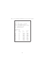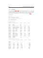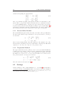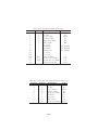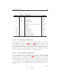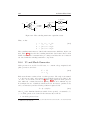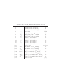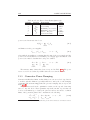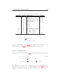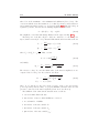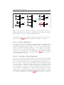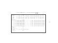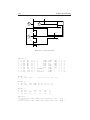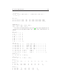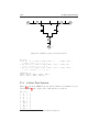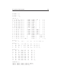
1
PSAT Power System Analysis Toolbox Documentation for PSAT version 2.0.0, February 14, 2008 Federico Milano c 2003 - 2008 Federico Milano Copyright Permission is granted to copy, distribute and/or modify this document under the terms of the GNU Free Documentation License, Version 1.1 or any later version published by the Free Software Foundation; with the Invariant Sections being all sections, with no Front-Cover Texts, and with no Back-Cover Texts. A copy of the license is included in Appendix L entitled “GNU Free Documentation License”. Ai miei genitori Note PSAT is a Matlab toolbox for static and dynamic analysis and control of electric power systems. I began writing PSAT in September 2001, while I was studying as Ph.D. student at the Universitá degli Studi di Genova, Italy, and completed the first public version in November 2002, when I was a Visiting Scholar at the University of Waterloo, Canada. I am currently maintaining PSAT in the spare time, while I am working as assistant professor at the Universidad de Castilla-La Mancha, Ciudad Real, Spain. PSAT is provided free of charge, in the hope it can be useful and other people can use and improve it, but please be aware that this toolbox comes with ABSOLUTELY NO WARRANTY; for details type warranty at the Matlab prompt. PSAT is free software, and you are welcome to redistribute it under certain conditions; for details refer to Appendix K of this documentation or type gnulicense at the Matlab prompt. PSAT is currently in a early stage of development and its features, structures and data formats may be partially or completely changed in future versions. Be sure to visit often my webpage in order to get the last version: http://www.uclm.es/area/gsee/Web/Federico/psat.htm If you find bugs or have any suggestions, please send me an e-mail at: [email protected] or you can subscribe to the PSAT Forum, which is available at: http://groups.yahoo.com/groups/psatforum Acknowledgements I wish to thank very much Professor C. A. Cañizares for his priceless help, teachings and advises. Thanks also for providing me a webpage and a link to my software in the main webpage of the E&CE Deparment, University of Waterloo, Canada. Many thanks to the moderators of the PSAT Forum for spending their time on answering tons of messages: Luigi Vanfretti, Juan Carlos Morataya, Raul Rabinovici, Ivo Šmon, and Zhen Wang. Thanks to Hugo M. Ayres, Marcelo S. Castro, Alberto Del Rosso, Jasmine, Igor Kopcak, Liu Lin, Lars Lindgren, Marcos Miranda, Juan Carlos Morataya, Difahoui Rachid, Santiago Torres, and Luigi Vanfretti for their relevant contributions, corrections and bug fixes. Contents I Outlines 1 1 Introduction 1.1 Overview . . . . . . . . . . . . . . 1.2 PSAT vs. Other Matlab Toolboxes 1.3 Outlines of the Manual . . . . . . . 1.4 Users . . . . . . . . . . . . . . . . . 2 Getting Started 2.1 Download . . . . . . . 2.2 Requirements . . . . . 2.3 Installation . . . . . . 2.4 Launching PSAT . . . 2.5 Loading Data . . . . . 2.6 Running the Program 2.7 Displaying Results . . 2.8 Saving Results . . . . 2.9 Settings . . . . . . . . 2.10 Network Design . . . . 2.11 Tools . . . . . . . . . . 2.12 Interfaces . . . . . . . 3 News 3.1 News 3.2 News 3.3 News 3.4 News 3.5 News 3.6 News 3.7 News 3.8 News 3.9 News 3.10 News 3.11 News in in in in in in in in in in in version version version version version version version version version version version 2.0.0 1.3.4 1.3.3 1.3.2 1.3.1 1.3.0 1.2.2 1.2.1 1.2.0 1.1.0 1.0.1 . . . . . . . . . . . . . . . . . . . . . . . . . . . . . . . . . . . . . . . . . . . . . . . . . . . . . . . . . . . . . . . . . . . . . . . . . . . . 3 3 6 6 7 . . . . . . . . . . . . . . . . . . . . . . . . . . . . . . . . . . . . . . . . . . . . . . . . . . . . . . . . . . . . . . . . . . . . . . . . . . . . . . . . . . . . . . . . . . . . . . . . . . . . . . . . . . . . . . . . . . . . . . . . . . . . . . . . . . . . . . . . . . . . . . . . . . . . . . . . . . . . . . . . . . . . . . . . . . . . . . . . . . . . . . . . . . . . . . . . . . . . . . . . . . . . . . . . . . . . . . . . . . . . . . . . . . . . . . . . . . . . . . . . . . . . . . . . . . . . . . . . . . . . . . . . . . . . . . . . . . . . . . . . . . . . . . . . . . . . . . . . . . . . 9 9 9 10 11 12 14 14 15 15 16 16 17 beta . . . . . . . . . . . . . . . . . . . . . . . . . . . . . . . . . . . . . . . . . . . . . . . . . . . . . . . . . . . . . . . . . . . . . . . . . . . . . . . . . . . . . . . . . . . . . . . . . . . . . . . . . . . . . . . . . . . . . . . . . . . . . . . . . . . . . . . . . . . . . . . . . . . . . . . . . . . . . . . . . . . . . . . . . . . . . . . . . . . . . . . . . . . . . . . . . . . . . . . . . . . . . . . . . . . . . . . . . . . . . . . . . . . . . . . . . . . . . . . . . . . . . . . . . . . . . . . . . . . . . . . . . . . . . . . . . . . . . . . . . . . . . . . . . . . . . . 19 19 20 21 21 21 22 22 23 23 23 23 . . . . . . . . . . . . vii viii II CONTENTS Routines 25 4 Power Flow 4.1 Power Flow Solvers . . . . . . . . . . . 4.1.1 Newton-Raphson Method . . . 4.1.2 Fast Decoupled Power Flow . . 4.1.3 Distributed Slack Bus Model . 4.1.4 Initialization of State Variables 4.2 Settings . . . . . . . . . . . . . . . . . 4.3 Example . . . . . . . . . . . . . . . . . . . . . . . . . . . . . . . . . . . . . . . . . . . . . . . . . . . . . . . . . . . . . . . . . . . . . . . . . . . . . . . . . . . . . . . . . . . . . . . . . . . . . . . . . . . . . . . . . . . 27 27 27 28 29 30 30 31 5 Bifurcation Analysis 5.1 Direct Methods . . . . . . . . . . . . . . . . . 5.1.1 Saddle-Node Bifurcation . . . . . . . . 5.1.2 Limit Induced Bifurcation . . . . . . . 5.2 Continuation Power Flow . . . . . . . . . . . 5.2.1 Predictor Step . . . . . . . . . . . . . 5.2.2 Corrector Step . . . . . . . . . . . . . 5.2.3 N-1 Contingency Analysis . . . . . . . 5.2.4 Graphical User Interface and Settings 5.3 Examples . . . . . . . . . . . . . . . . . . . . . . . . . . . . . . . . . . . . . . . . . . . . . . . . . . . . . . . . . . . . . . . . . . . . . . . . . . . . . . . . . . . . . . . . . . . . . . . . . . . . . . . . . . . . . . . . . . . . . . . . . . . . . . . . . . . . . . . . . 39 40 40 40 41 43 43 44 45 46 6 Optimal Power Flow 6.1 Interior Point Method . . . . . . . . . . . . . . . 6.2 OPF Routines . . . . . . . . . . . . . . . . . . . . 6.2.1 Maximization of the Social Benefit . . . . 6.2.2 Maximization of the Distance to Collapse 6.2.3 Multi-Objective Optimization . . . . . . . 6.2.4 Lagrangian Function . . . . . . . . . . . . 6.3 OPF Settings . . . . . . . . . . . . . . . . . . . . 6.4 Example . . . . . . . . . . . . . . . . . . . . . . . . . . . . . . . . . . . . . . . . . . . . . . . . . . . . . . . . . . . . . . . . . . . . . . . . . . . . . . . . . . . . . . . . . . . . . . . . . . . . . . . . . . . . . . . 53 53 54 54 54 56 57 57 58 7 Small Signal Stability Analysis 7.1 Small Signal Stability Analysis . 7.1.1 Example . . . . . . . . . . 7.2 Power Flow Sensitivity Analysis . 7.2.1 Example . . . . . . . . . . 7.3 Graphical User Interface . . . . . . . . . . . . . . . . . . . . . . . . . . . . . . . . . . . . . . . . . . . . . . . . . . . . . . . . . . . . . . . . . . . . . . . . . . . . . . . . . . . . . . . . . . . . . . . . . . . . . . . . . 63 63 66 69 70 72 8 Time Domain Simulation 8.1 Integration Methods . . . . . 8.1.1 Forward Euler Method 8.1.2 Trapezoidal Method . 8.2 Settings . . . . . . . . . . . . 8.3 Output Variable Selection . . 8.4 Snapshots . . . . . . . . . . . . . . . . . . . . . . . . . . . . . . . . . . . . . . . . . . . . . . . . . . . . . . . . . . . . . . . . . . . . . . . . . . . . . . . . . . . . . . . . . . . . . . . . . . . . . . . . . . . . . . . . . . . . . . . . . . . . . . . . . . . 75 75 76 76 76 79 82 . . . . . . . . . . . . . . . . . . . . . . . . . . . . . . . . . CONTENTS 8.5 8.6 ix Disturbances . . . . . . . . . . . . . . . . . . . . . . . . . . . . . . . Examples . . . . . . . . . . . . . . . . . . . . . . . . . . . . . . . . . 9 PMU Placement 9.1 Linear Static State Estimation . . . . . . 9.2 PMU Placement Rules . . . . . . . . . . . 9.3 Algorithms . . . . . . . . . . . . . . . . . 9.3.1 Depth First . . . . . . . . . . . . . 9.3.2 Graph Theoretic Procedure . . . . 9.3.3 Bisecting Search Method . . . . . 9.3.4 Recursive Security N Algorithm . . 9.3.5 Single Shot Security N Algorithm . 9.3.6 Recursive and Single-Shot Security 9.4 PMU Placement GUI and Settings . . . . 9.4.1 Example . . . . . . . . . . . . . . . III . . . . . . . . . . . . . . . . . . . . . . . . . . . . . . . . . . . . . . . . . . . . . . . . . . . . . . . . . . . . . . . . . . . . . . . . N-1 Algorithms . . . . . . . . . . . . . . . . . . . . . . . . . . . . . . . . . . . . . . . . . . . . . . . . . . . . . . . . . . . . . . . . . . . . . . . . . Models . . . . . . . . . . . 82 84 89 89 90 90 90 91 91 91 92 92 97 97 101 10 Power Flow Data 10.1 Bus . . . . . . . . . . . . . . . . . . 10.2 Transmission Line . . . . . . . . . . 10.3 Transformers . . . . . . . . . . . . . 10.3.1 Two-Winding Transformers . 10.3.2 Three-Winding Transformers 10.4 Vθ and Slack Generator . . . . . . . 10.5 PV Generator . . . . . . . . . . . . . 10.6 PQ Load . . . . . . . . . . . . . . . . 10.7 PQ Generator . . . . . . . . . . . . . 10.8 Shunt . . . . . . . . . . . . . . . . . 10.9 Area & Regions . . . . . . . . . . . . . . . . . . . . . . . . . . . . . . . . . . . . . . . . . . . . . . . . . . . . . . . . . . . . . . . . . . . . . . . . . . . . . . . . . . . . . . . . . . . . . . . . . . . . . . . . . . . . . . . . . . . . . . . . . . . . . . . . . . . . . . . . . . . . . . . . . . . . . . . . . . . . . . . . . . . . . . . . . . . . . . . . . . . . . . . . . . . . . . . . . . . . . . . . . . . . . . . . . . 103 103 104 105 107 107 108 110 111 113 113 114 11 CPF and OPF Data 11.1 Generator Supply . . . . . 11.2 Generator Reserve . . . . 11.3 Generator Power Ramping 11.4 Load Demand . . . . . . . 11.5 Demand Profile . . . . . . 11.6 Load Ramping . . . . . . . . . . . . . . . . . . . . . . . . . . . . . . . . . . . . . . . . . . . . . . . . . . . . . . . . . . . . . . . . . . . . . . . . . . . . . . . . . . . . . . . . . . . . . . . . . . . . . . . . . . . . . . . . . . 117 118 119 120 121 122 124 . . . . . . . . . . . . . . . . . . . . . . . . . . . . . . . . . . . . 12 Faults & Breakers 127 12.1 Fault . . . . . . . . . . . . . . . . . . . . . . . . . . . . . . . . . . . . 127 12.2 Breaker . . . . . . . . . . . . . . . . . . . . . . . . . . . . . . . . . . 127 13 Measurements 131 13.1 Bus Frequency Measurement . . . . . . . . . . . . . . . . . . . . . . 131 x CONTENTS 13.2 Phasor Measurement Unit . . . . . . . . . . . . . . . . . . . . . . . . 132 14 Loads 14.1 Voltage Dependent Load . . . . . . . 14.2 ZIP Load . . . . . . . . . . . . . . . 14.3 Frequency Dependent Load . . . . . 14.4 Exponential Recovery Load . . . . . 14.5 Thermostatically Controlled Load . . 14.6 Jimma’s Load . . . . . . . . . . . . . 14.7 Mixed Load . . . . . . . . . . . . . . 14.8 Note on the Use of Non-conventional . . . . . . . . . . . . . . . . . . . . . . . . . . . . Loads . . . . . . . . . . . . . . . . . . . . . . . . . . . . . . . . . . . . . . . . . . . . . . . . . . . . . . . . . . . . . . . . . . . . . . . . . . . . . . . . . . . . . . . . . . . . . . . . . . . . . . . . . . . . . . . . 135 135 136 137 138 140 142 143 144 15 Machines 15.1 Synchronous Machine . . . . 15.1.1 Order II . . . . . . . . 15.1.2 Order III . . . . . . . 15.1.3 Order IV . . . . . . . 15.1.4 Order V, Type 1 . . . 15.1.5 Order V, Type 2 . . . 15.1.6 Order V, Type 3 . . . 15.1.7 Order VI . . . . . . . 15.1.8 Order VIII . . . . . . 15.1.9 Center of Inertia . . . 15.2 Induction Motor . . . . . . . 15.2.1 Order I . . . . . . . . 15.2.2 Order III (single cage) 15.2.3 Order V (double cage) . . . . . . . . . . . . . . . . . . . . . . . . . . . . . . . . . . . . . . . . . . . . . . . . . . . . . . . . . . . . . . . . . . . . . . . . . . . . . . . . . . . . . . . . . . . . . . . . . . . . . . . . . . . . . . . . . . . . . . . . . . . . . . . . . . . . . . . . . . . . . . . . . . . . . . . . . . . . . . . . . . . . . . . . . . . . . . . . . . . . . . . . . . . . . . . . . . . . . . . . . . . . . . . . . . . . . . . . . . . . . . . . . . . . . . . . . . . . . . . . . . . . . . . . . . . . . . . . . . . . . . . . . . . . . . . . . . . . . . . . . . . . . . . . . . . . . . . . . . . . . . . . . . . . 147 147 154 154 154 155 155 156 157 157 158 158 159 161 162 16 Controls 16.1 Turbine Governor . . . . . . . 16.1.1 TG Type I . . . . . . 16.1.2 TG Type II . . . . . . 16.2 Automatic Voltage Regulator 16.2.1 AVR Type I . . . . . . 16.2.2 AVR Type II . . . . . 16.2.3 AVR Type III . . . . . 16.3 Power System Stabilizer . . . 16.3.1 Type I . . . . . . . . . 16.3.2 Type II . . . . . . . . 16.3.3 Type III . . . . . . . . 16.3.4 Type IV and V . . . . 16.4 Over Excitation Limiter . . . 16.5 Secondary Voltage Control . . 16.6 Power Oscillation Damper . . . . . . . . . . . . . . . . . . . . . . . . . . . . . . . . . . . . . . . . . . . . . . . . . . . . . . . . . . . . . . . . . . . . . . . . . . . . . . . . . . . . . . . . . . . . . . . . . . . . . . . . . . . . . . . . . . . . . . . . . . . . . . . . . . . . . . . . . . . . . . . . . . . . . . . . . . . . . . . . . . . . . . . . . . . . . . . . . . . . . . . . . . . . . . . . . . . . . . . . . . . . . . . . . . . . . . . . . . . . . . . . . . . . . . . . . . . . . . . . . . . . . . . . . . . . . . . . . . . . . . . . . . . . . . . . . . . . . . . . . . . . . . . . . . . . . . . . . . . . . . . . . . . . . . . . . . . . . . . . . . . . . . . . . . . . 165 165 166 168 169 169 170 171 174 176 176 177 177 177 180 183 17 Regulating Transformers 185 CONTENTS xi 17.1 Under Load Tap Changer . . . . . . . . . . . . . . . . . . . . . . . . 185 17.2 Load Tap Changer With Embedded Load . . . . . . . . . . . . . . . 186 17.3 Phase Shifting Transformer . . . . . . . . . . . . . . . . . . . . . . . 189 18 FACTS 18.1 SVC . . . . 18.2 TCSC . . . 18.3 STATCOM 18.4 SSSC . . . . 18.5 UPFC . . . 18.6 HVDC . . . . . . . . . . . . . . . . . . . . . . . . . . . . . . . . . . . . . . . . . . . . . . . . . . . . . . . . . . . . . . . . . . . . . . . . . . . . . . . . . . . . . . . . . . . . . 193 194 196 198 201 204 209 19 Wind Turbines 19.1 Wind Models . . . . . . . . . . . . . . . . . 19.1.1 Weibull Distribution . . . . . . . . . 19.1.2 Composite Wind Model . . . . . . . 19.1.3 Measurement Data . . . . . . . . . . 19.2 Wind Turbines . . . . . . . . . . . . . . . . 19.2.1 Constant Speed Wind Turbine . . . 19.2.2 Doubly Fed Induction Generator . . 19.2.3 Direct Drive Synchronous Generator . . . . . . . . . . . . . . . . . . . . . . . . . . . . . . . . . . . . . . . . . . . . . . . . . . . . . . . . . . . . . . . . . . . . . . . . . . . . . . . . . . . . . . . . . . . . . . . . . . . . . . . . . . . . . . . . 213 213 214 216 217 217 219 221 227 . . . . . . . . . . . . . . . . . . . . . . . . . . . . . . . . . . . . . . . . . . . . . . . . . . . . . . . . . . . . . . . . . . . . . . . . . . . . . . . . . . . . . . . . . . . . . . . . . . . . . . 20 Other Models 231 20.1 Dynamic Shaft . . . . . . . . . . . . . . . . . . . . . . . . . . . . . . 231 20.2 Sub-synchronous Resonance Model . . . . . . . . . . . . . . . . . . . 233 20.3 Solid Oxide Fuel Cell . . . . . . . . . . . . . . . . . . . . . . . . . . . 236 IV CAD 243 21 Network Design 21.1 Simulink Library . . . . . . . . . . . . 21.2 Extracting Data from Simulink Models 21.3 Displaying Results in Simulink Models 21.4 Examples . . . . . . . . . . . . . . . . . . . . . . . . . . . . . . . . . . . . . . . . . . . . . . . . . . . . . . . . . . . . . . . . . . . . . . . . . . . . . . . . . . . . 245 245 245 253 253 22 Block Usage 22.1 Block Connections . . . . . . . . . . 22.2 Standard Blocks . . . . . . . . . . . 22.3 Nonstandard Blocks . . . . . . . . . 22.3.1 Buses . . . . . . . . . . . . . 22.3.2 Goto and From Blocks . . . . 22.3.3 Links . . . . . . . . . . . . . 22.3.4 Breakers . . . . . . . . . . . . 22.3.5 Power Supplies and Demands 22.3.6 Generator Ramping . . . . . . . . . . . . . . . . . . . . . . . . . . . . . . . . . . . . . . . . . . . . . . . . . . . . . . . . . . . . . . . . . . . . . . . . . . . . . . . . . . . . . . . . . . . . . . . . . . . . . . . . . . . . . . . . . . . . . . . . . . . . . . . . . . . . . . . . . . . . . . . . . . . . . . . . . . . . . . 257 257 258 260 260 260 260 261 262 262 . . . . . . . . . xii CONTENTS 22.3.7 Generator Reserves . . . . . . 22.3.8 Non-conventional Loads . . . 22.3.9 Synchronous Machines . . . . 22.3.10 Primary Regulators . . . . . 22.3.11 Secondary Voltage Regulation 22.3.12 Under Load Tap Changers . . 22.3.13 SVCs & STATCOMs . . . . . 22.3.14 Solid Oxide Fuel Cells . . . . 22.3.15 Dynamic Shafts . . . . . . . . . . . . . . . . . . . . . . . . . . . . . . . . . . . . . . . . . . . . . . . . . . . . . . . . . . . . . . . . . . . . . . . . . . . . . . . . . . . . . . . . . . . . . . . . . . . . . . . . . . . . . . . . . . . . . . . . . . . . . . . . . . . . . . . . . . . . . . . . . . . . . . . . . . . . . . . . . . . . . . . . . . 262 262 264 265 265 266 266 268 268 23 Block Masks 23.1 Blocks vs. Global Structures . . . . 23.2 Editing Block Masks . . . . . . . . . 23.2.1 Mask Initialization . . . . . . 23.2.2 Mask Icon . . . . . . . . . . . 23.2.3 Mask Documentation . . . . 23.3 Syntax of Mask Parameter Names . 23.4 Remarks on Creating Custom Blocks . . . . . . . . . . . . . . . . . . . . . . . . . . . . . . . . . . . . . . . . . . . . . . . . . . . . . . . . . . . . . . . . . . . . . . . . . . . . . . . . . . . . . . . . . . . . . . . . . . . . . . . . . . . . . . . . . . . . . . . . . . . . . . 271 271 272 272 274 276 276 277 V Tools 281 24 Data Format Conversion 283 25 User Defined Models 25.1 Installing and Removing Models 25.2 Creating a User Defined Model . 25.2.1 Component Settings . . . 25.2.2 State Variable Settings . . 25.2.3 Parameter Settings . . . . 25.3 Limitations . . . . . . . . . . . . . . . . . . . . . . . . . . . . . . . . . . . . . . . . . . . . . . . . . . . . . . . . . . . . . . . . . . . . . . . . . . . . . . . . . . . . . . . . . . . . . . . . . . . . . . . . . . . . . . . . . . . . . . . . . . . . . . . . . . . . 287 287 289 289 293 294 294 26 Utilities 26.1 Command History . . . . . 26.2 Sparse Matrix Visualization 26.3 Themes . . . . . . . . . . . 26.4 Text Viewer . . . . . . . . . 26.5 Building p-code Archive . . . . . . . . . . . . . . . . . . . . . . . . . . . . . . . . . . . . . . . . . . . . . . . . . . . . . . . . . . . . . . . . . . . . . . . . . . . . . . . . . . . . . . . . . . . . . . . . . . . . . . . . . . . . . . . . . . . . . 295 295 295 295 295 296 27 Command Line Usage 27.1 Basics . . . . . . . . . . 27.2 Advanced Usage . . . . 27.3 Command Line Options 27.4 Example . . . . . . . . . . . . . . . . . . . . . . . . . . . . . . . . . . . . . . . . . . . . . . . . . . . . . . . . . . . . . . . . . . . . . . . . . . . . . . . . . . . . . . . . . . . . . . . . . . . . . 301 301 304 305 306 . . . . . . . . 28 Running PSAT on GNU Octave 309 28.1 Basic Commands . . . . . . . . . . . . . . . . . . . . . . . . . . . . . 310 CONTENTS xiii 28.2 Plot Variables . . . . . . . . . . . . . . . . . . . . . . . . . . . . . . . 310 28.3 ToDos . . . . . . . . . . . . . . . . . . . . . . . . . . . . . . . . . . . 312 VI Interfaces 313 29 GAMS Interface 29.1 Getting Started . . . . . . . . . . . . . . . 29.2 GAMS Solvers . . . . . . . . . . . . . . . 29.3 PSAT-GAMS Interface . . . . . . . . . . . 29.4 PSAT-GAMS Models . . . . . . . . . . . . 29.5 Multiperiod Market Clearing Model . . . 29.5.1 Notation . . . . . . . . . . . . . . . 29.5.2 Model Equations and Constraints . 29.6 Example . . . . . . . . . . . . . . . . . . . . . . . . . . . . . . . . . . . . . . . . . . . . . . . . . . . . . . . . . . . . . . . . . . . . . . . . . . . . . . . . . . . . . . . . . . . . . . . . . . . . . . . . . . . . . . . . . . . . . . . . . . . . . . . . . . . . . . . . . . . 315 315 316 316 317 320 320 321 323 30 UWPFLOW Interface 30.1 Getting Started . . . . . 30.2 Graphical User Interface 30.3 Limitations and ToDos . 30.4 Example . . . . . . . . . . . . . . . . . . . . . . . . . . . . . . . . . . . . . . . . . . . . . . . . . . . . . . . . . . . . . . . . . . . . . 331 331 332 332 334 VII . . . . . . . . . . . . . . . . . . . . . . . . . . . . . . . . . . . . . . . . Libraries 339 31 Numeric Linear Analysis 31.1 Description . . . . . . . . . . . . . . . . . . . . . . . . . . 31.2 Test cases . . . . . . . . . . . . . . . . . . . . . . . . . . . 31.2.1 Comparison of state matrices . . . . . . . . . . . . 31.2.2 Results for a change of an exciter reference voltage 31.2.3 Results for a change of governor reference speeds . 31.2.4 Results for a change of a SVC reference voltage . . VIII . . . . . . . . . . . . . . . . . . . . . . . . . . . . . . Appendices A Global Structures & Classes A.1 General Settings . . . . . . . . A.2 Other Settings . . . . . . . . . A.3 System Properties and Settings A.4 Outputs and Variable Names . A.5 User Defined Models . . . . . . A.6 Models . . . . . . . . . . . . . . A.7 Command Line Usage . . . . . A.8 Interfaces . . . . . . . . . . . . A.9 Classes . . . . . . . . . . . . . . . . . . . . 341 341 342 343 343 344 347 351 . . . . . . . . . . . . . . . . . . . . . . . . . . . . . . . . . . . . . . . . . . . . . . . . . . . . . . . . . . . . . . . . . . . . . . . . . . . . . . . . . . . . . . . . . . . . . . . . . . . . . . . . . . . . . . . . . . . . . . . . . . . . . . . . . . . . . . . . . . . . . . . . . . . . . . . . . . . . . . . . . . . . . . . . . . . . . . . . . . . . . . . . . . . . . 353 353 357 360 366 366 368 370 371 372 xiv CONTENTS B Matlab Functions 375 C Other Files and Folders 381 D Third Party Matlab Code 385 E Power System Softwares 387 F Test System Data F.1 3-bus Test System F.2 6-bus Test System F.3 9-bus Test System F.4 14-bus Test System . . . . . . . . . . . . . . . . . . . . . . . . . . . . . . . . . . . . . . . . . . . . . . . . . . . . . . . . . . . . . . . . . . . . . . . . . . . . 389 389 390 391 394 G FAQs G.1 Getting Started . . . . . . . . . . . . G.2 Simulink Library . . . . . . . . . . . G.3 Power Flow . . . . . . . . . . . . . . G.4 Optimal & Continuation Power Flow G.5 Time Domain Simulation . . . . . . G.6 Data Conversion . . . . . . . . . . . G.7 Interfaces . . . . . . . . . . . . . . . . . . . . . . . . . . . . . . . . . . . . . . . . . . . . . . . . . . . . . . . . . . . . . . . . . . . . . . . . . . . . . . . . . . . . . . . . . . . . . . . . . . . . . . . . . . . . . . . . . . . . . . . . . . . . . . . . . . . . . . . . . . . . . 397 397 399 400 401 401 402 403 . . . . . . . . . . . . . . . . . . . . . . . . . . . . . . . . . . . . H PSAT Forum I Citations & Links I.1 Books . . . . . . . . . . I.2 Journals . . . . . . . . . I.3 Conference Proceedings I.4 Webpages . . . . . . . . 405 . . . . . . . . . . . . . . . . . . . . . . . . . . . . . . . . . . . . . . . . . . . . . . . . . . . . . . . . . . . . . . . . . . . . . . . . . . . . . . . . . . . . . . . . . . . . . . . . . . . . 409 409 409 410 410 J Letters of Reference 413 K The GNU General Public License 417 L GNU Free Documentation License 425 Bibliography 443 List of Figures 1.1 1.2 PSAT at a glance. . . . . . . . . . . . . . . . . . . . . . . . . . . . PSAT around the world. . . . . . . . . . . . . . . . . . . . . . . . . 5 8 2.1 Main graphical user interface of PSAT. . . . . . . . . . . . . . . . 13 4.1 4.2 4.3 4.4 GUI for general settings. . . . . . . . . GUI for displaying power flow results. 2D visualization of power flow results. 3D visualization of power flow results. . . . . . . . . . . . . . . . . . . . . . . . . . . . . . . . . 32 33 37 38 5.1 5.2 5.3 5.4 5.5 5.6 5.7 5.8 5.9 GUI for saddle-node bifurcation settings. . . . . . . . GUI for limit-induced bifurcation settings. . . . . . . . Continuation Power Flow: tangent vector . . . . . . . Continuation Power Flow: perpendicular intersection . Continuation Power Flow: local parametrization . . . GUI for the continuation power flow settings. . . . . . GUI for plotting CPF results. . . . . . . . . . . . . . . Nose curves for the 6-bus test system (LIB) . . . . . . Nose curves for the 6-bus test system (SNB) . . . . . . . . . . . . . . . . . . . . . . . . . . . . . . . . . . . . . . . . . . . . . . . . . . . . . . . . . . . . . . . . . . . . 41 42 43 44 45 47 48 49 50 6.1 6.2 6.3 GUI for the optimal power flow. . . . . . . . . . . . . . . . . . . . GUI for displaying OPF results. . . . . . . . . . . . . . . . . . . . GUI for plotting OPF Pareto sets. . . . . . . . . . . . . . . . . . . 58 59 62 7.1 7.2 7.3 7.4 Eigenvalue Analysis: S-domain. . . . . . . Eigenvalue Analysis: Z-domain. . . . . . Eigenvalue Analysis: QV sensitivity. . . . GUI for the small signal stability analysis. . . . . . . . . . . . . . . . . . . . . . . . . . . . . . . . . . . . . . . . . . . . . 65 65 70 73 8.1 8.2 8.3 8.4 8.5 8.6 8.7 Time domain integration block diagram. . . . . . GUI for general settings. . . . . . . . . . . . . . . GUI for plot variable selection. . . . . . . . . . . Snapshot GUI. . . . . . . . . . . . . . . . . . . . GUI for plotting time domain simulations. . . . . Generator speeds for the 9-bus test system. . . . Generator rotor angles for the 9-bus test system. . . . . . . . . . . . . . . . . . . . . . . . . . . . . . . . . . . . . . . . . . . . . . . . . . . . . . . . . . . . . . . . . . . . . . . 77 79 81 82 85 86 87 xv . . . . . . . . . . . . . . . . . . . . . . . . . . . . . . . . . . . . . . . . . . . . xvi LIST OF FIGURES 8.8 Bus voltages for the 9-bus test system. . . . . . . . . . . . . . . . . 88 9.1 9.2 9.3 9.4 9.5 9.6 9.7 9.8 9.9 9.10 9.11 PMU placement rules. . . . . . . . . . . . . . . . . . Flowchart of the Graph Theoretic Procedure. . . . . Flowchart of the Bisecting Search. . . . . . . . . . . Pseudo-code of the simulated Annealing Algorithm. Recursive N Security Method. . . . . . . . . . . . . . Search of alternative placement sets. . . . . . . . . . Pure transit node filtering. . . . . . . . . . . . . . . Single-Shot N Security Method. . . . . . . . . . . . . Recursive N-1 Security Method. . . . . . . . . . . . Single Shot N-1 Security Method. . . . . . . . . . . GUI for the PMU placement methods. . . . . . . . . 91 92 93 94 95 95 95 96 97 98 99 10.1 10.2 Transmission line π circuit. . . . . . . . . . . . . . . . . . . . . . . 105 Three-winding transformer equivalent circuit. . . . . . . . . . . . . 108 11.1 Example of daily demand profile. . . . . . . . . . . . . . . . . . . . 125 13.1 13.2 Bus frequency measurement filter. . . . . . . . . . . . . . . . . . . 131 Phasors from sample data. . . . . . . . . . . . . . . . . . . . . . . 133 14.1 14.2 14.3 Measure of frequency deviation. . . . . . . . . . . . . . . . . . . . . 138 Thermostatically controlled load. . . . . . . . . . . . . . . . . . . . 141 Jimma’s load. . . . . . . . . . . . . . . . . . . . . . . . . . . . . . . 142 15.1 15.2 15.3 15.4 15.5 15.6 Synchronous machine scheme. . . . . . . . . . . . . . . . Synchronous machine: block diagram of stator fluxes. . Field saturation characteristic of synchronous machines. Order I induction motor: electrical circuit. . . . . . . . Order III induction motor: electrical circuit. . . . . . . Order V induction motor: electrical circuit. . . . . . . . . . . . . . . . . . . . . . . . . . . . . . . . . . . . . . . . . . . . 150 151 152 161 162 163 16.1 16.2 16.3 16.4 16.5 16.6 16.7 16.8 16.9 16.10 16.11 16.12 Turbine governor type I. . . . . . . Turbine governor type II. . . . . . Exciter Type I. . . . . . . . . . . . Exciter Type II. . . . . . . . . . . Exciter Type III. . . . . . . . . . . Power system stabilizer Type I. . . Power system stabilizer Type II. . Power system stabilizer Type III. . Power system stabilizer Type IV. . Power system stabilizer Type V. . Over excitation limiter. . . . . . . Secondary voltage control scheme. . . . . . . . . . . . . . . . . . . . . . . . . . . . . . . . . . . . . . . . . . . . . . . . . . . . . . . . . . . . . . . . . . . . . . . . . 167 168 170 172 173 176 176 177 178 178 180 182 17.1 Under Load Tap Changer: equivalent π circuit. . . . . . . . . . . . 187 . . . . . . . . . . . . . . . . . . . . . . . . . . . . . . . . . . . . . . . . . . . . . . . . . . . . . . . . . . . . . . . . . . . . . . . . . . . . . . . . . . . . . . . . . . . . . . . . . . . . . . . . . . . . . . . . . . . . . . . . . . . . . . . . . . . . . . . . . . . . . . . . . . . . . . . . . . . . . . . . . . . . . . . . . . . . . . . . . . . . . . . . . . . . . . . . . . . . . . . . . . . . . . . . . . . . . . . . . . . . . . . . . . . . . . . . LIST OF FIGURES xvii 17.2 17.3 17.4 17.5 Under Load Tap Changer: voltage and reactive Load Tap Changer with embedded load. . . . . Phase shifting transformer circuit. . . . . . . . Phase shifting transformer control scheme. . . power controls. . . . . . . . . . . . . . . . . . . . . . . . . . . . . . . . . . . . 187 189 191 191 18.1 18.2 18.3 18.4 18.5 18.6 18.7 18.8 18.9 18.10 18.11 SVC Type 1 Regulator. . . . . . . . SVC Type 2 Regulator. . . . . . . . TCSC Regulator. . . . . . . . . . . . STATCOM circuit and control block SSSC circuit. . . . . . . . . . . . . . SSSC control block diagram. . . . . UPFC circuit. . . . . . . . . . . . . . UPFC phasor diagram. . . . . . . . UPFC control block diagrams. . . . HVDC scheme. . . . . . . . . . . . . HVDC current control. . . . . . . . . . . . . . . . . . . . . . . . . . . . . . . . . . . . . . . . . . . . . . . . . . . . . . . . . . . . . . . . . . . . . . . . . . . . . . . . . . . . . . . . . . . . . . . . . . . . . . . . . . . . . . . . . . . . . . . . . . . . . . . . . 194 195 197 200 202 203 206 206 207 210 211 19.1 19.2 19.3 19.4 19.5 19.6 Low-pass filter to smooth wind speed variations. Wind turbine types . . . . . . . . . . . . . . . . Rotor speed control scheme. . . . . . . . . . . . . Voltage control scheme. . . . . . . . . . . . . . . Power-speed characteristic. . . . . . . . . . . . . Pitch angle control scheme. . . . . . . . . . . . . . . . . . . . . . . . . . . . . . . . . . . . . . . . . . . . . . . . . . . . . . . . . . . . . . . . . . . . . . . . . 214 218 224 225 225 225 20.1 20.2 20.3 20.4 20.5 Synchronous machine mass-spring shaft model. . . . . Generator with dynamic shaft and compensated line. . Solid Oxide Fuel Cell scheme. . . . . . . . . . . . . . . Solid Oxide Fuel Cell connection with the AC grid. . . AC voltage control for the Solid Oxide Fuel Cell. . . . . . . . . . . . . . . . . . . . . . . . . . . . . . . . . . . . . . . 232 234 239 241 241 21.1 21.2 21.3 21.4 21.5 21.6 21.7 21.8 21.9 21.10 21.11 21.12 21.13 21.14 21.15 21.16 Simulink library: Main Window. . . . . . . . . . . . . . . . . Simulink library: Connections. . . . . . . . . . . . . . . . . . Simulink library: Power Flow data. . . . . . . . . . . . . . . . Simulink library: OPF & CPF data. . . . . . . . . . . . . . . Simulink library: Faults & Breakers. . . . . . . . . . . . . . . Simulink library: Measurements. . . . . . . . . . . . . . . . . Simulink library: Loads. . . . . . . . . . . . . . . . . . . . . . Simulink library: Machines. . . . . . . . . . . . . . . . . . . . Simulink library: Regulators. . . . . . . . . . . . . . . . . . . Simulink library: Regulating Transformers. . . . . . . . . . . Simulink library: FACTS controllers. . . . . . . . . . . . . . . Simulink library: Wind Turbines. . . . . . . . . . . . . . . . . Simulink library: Other models. . . . . . . . . . . . . . . . . GUI for Simulink model settings. . . . . . . . . . . . . . . . . Simulink model of the WSCC 3-generator 9-bus test system. Simulink model of the IEEE 14-bus test system. . . . . . . . . . . . . . . . . . . . . . . . . . . . . . . . . . . . . . . . . . . . . . . . . . . . . . . . 246 246 247 248 248 248 249 249 250 250 251 252 252 253 254 255 . . . . . . . . . . . . . . . . . . diagram. . . . . . . . . . . . . . . . . . . . . . . . . . . . . . . . . . . . . . . . . . . xviii LIST OF FIGURES 21.17 Simulink model of the 6-bus test system. . . . . . . . . . . . . . . 256 22.1 22.2 22.3 22.4 22.5 22.6 22.7 22.8 22.9 22.10 22.11 22.12 22.13 22.14 22.15 22.16 22.17 22.18 Examples of standard blocks of the PSAT Simulink Examples of allowed connections. . . . . . . . . . . . Examples of not allowed connections. . . . . . . . . Examples of infeasible connections. . . . . . . . . . . Bus block usage. . . . . . . . . . . . . . . . . . . . . Goto and From block usage. . . . . . . . . . . . . . . Breaker block usage. . . . . . . . . . . . . . . . . . . Supply and Demand block usage. . . . . . . . . . . . Generator Ramping block usage. . . . . . . . . . . . Generator Reserve block usage. . . . . . . . . . . . . Non-conventional Load block usage. . . . . . . . . . Synchronous Machine block usage. . . . . . . . . . . Primary Regulator block usage. . . . . . . . . . . . . Secondary Voltage Regulation block usage. . . . . . Under Load Tap Changer block usage. . . . . . . . . SVC block usage. . . . . . . . . . . . . . . . . . . . . Solid Oxide Fuel Cell block usage. . . . . . . . . . . Dynamic Shaft block usage. . . . . . . . . . . . . . . 23.1 23.2 23.3 23.4 23.5 23.6 Simulink blocks vs. PSAT global structures . . . . . Mask GUI of a PSAT-Simulink block. . . . . . . . . Mask initialization GUI for a PSAT-Simulink block. Mask icon GUI of a PSAT-Simulink block. . . . . . . Mask documentation GUI of a PSAT-Simulink block. Simulink model underneath a mask of a PSAT block. 24.1 GUI for data format conversion. . . . . . . . . . . . . . . . . . . . 285 25.1 25.2 25.3 25.4 25.5 Browser of user defined models. . . . . . . GUI for creating user defined models. . . GUI for setting component properties. . . GUI for setting state variable properties. GUI for setting parameters properties. . . . . . . . . . . . . . . . . . . . . . . . . . . . . . . . . . . . . . . . . . . . . . . . . . . . . . . . . . . . . . . . . . . . . . . . . 288 290 291 292 293 26.1 26.2 26.3 26.4 26.5 Command history GUI. . . . . . . . GUI for sparse matrix visualization. GUI for PSAT theme selection. . . . GUI for text viewer selection. . . . . GUI for p-code archive builder. . . . . . . . . . . . . . . . . . . . . . . . . . . . . . . . . . . . . . . . . . . . . . . . . . . . . . . . . . . . . . . . . . . . . . . . . . 296 297 298 299 299 27.1 Master-slave architecture. . . . . . . . . . . . . . . . . . . . . . . . 304 28.1 Example of graph obtained using GNU/Octave and gplot. . . . . . 311 29.1 Structure of the PSAT-GAMS interface. . . . . . . . . . . . . . . . 318 . . . . . . . . . . . . . . . Library. . . . . . . . . . . . . . . . . . . . . . . . . . . . . . . . . . . . . . . . . . . . . . . . . . . . . . . . . . . . . . . . . . . . . . . . . . . . . . . . . . . . . . . . . . . . . . . . . . . . . . . . . . . . . . . . . . . . . . . . . . . . . . . . . . . . . . . . . . . . . . . . . . . . . . . . . . . . . . . . . . . . 258 259 259 259 260 261 261 262 263 263 264 265 266 267 267 268 268 269 . . . . . . . . . . . . . . . . . . 272 273 274 275 276 279 LIST OF FIGURES xix 29.2 29.3 29.4 29.5 29.6 GUI of the PSAT-GAMS interface. . . . . . . . . . . PSAT-Simulink model of the three-bus test system. Demand profile for the multiperiod auction. . . . . . max limits. . . . . . . Multiperiod auction without Pmn max Multiperiod auction with Pmn limits. . . . . . . . . 30.1 30.2 GUI of the PSAT-UWPFLOW interface. . . . . . . . . . . . . . . 333 UWPFLOW nose curves for the 6-bus test systems. . . . . . . . . 338 31.1 31.2 31.3 31.4 31.5 31.6 31.7 31.8 Comparison of voltages at buses 6 and 7. . . . . . . . . . Comparison of reactive powers flows in lines 2-7 and 6-4. Comparison of active powers flows in line 2-7. . . . . . . . Comparison of rotor speeds. . . . . . . . . . . . . . . . . . Detail of the comparison of rotor speeds. . . . . . . . . . Comparison of active powers flows in line 2-7. . . . . . . . Comparison of SVC state variables. . . . . . . . . . . . . Comparison of voltages at bus 8. . . . . . . . . . . . . . . . . . . . . . . . . . . . . . . . . . . . . . . . . . . . . . . . . . . . . . . 345 345 346 348 348 349 350 350 F.1 F.2 F.3 F.4 3-bus test system. . . . . . . 6-bus test system. . . . . . . WSCC 3-generator 9-bus test IEEE 14-bus test system. . . . . . . . . . . . . . . . . . . . . . . 390 392 394 396 H.1 H.2 PSAT Forum main page . . . . . . . . . . . . . . . . . . . . . . . . 406 PSAT Forum statistics . . . . . . . . . . . . . . . . . . . . . . . . . 407 . . . . . . . . . . system. . . . . . . . . . . . . . . . . . . . . . . . . . . . . . . . . . . . . . . . . . . . . . . . . . . . . . . . . . . . . . . . . . . . . . . . . . . . . . . . . . . . . . . . . . 319 324 328 329 330 List of Tables 1.1 Matlab-based packages for power system analysis . . . . . . . . . . 5.1 N-1 Contingency Analysis Report 10.1 10.2 10.3 10.4 10.5 10.6 10.7 10.8 10.9 10.10 10.11 Bus Data Format . . . . . . . . . . . . . . Line Data Format . . . . . . . . . . . . . Alternative Line Data Format . . . . . . . Transformer Data Format . . . . . . . . . Three-Winding Transformer Data Format Slack Generator Data Format . . . . . . . PV Generator Data Format . . . . . . . . PQ Load Data Format . . . . . . . . . . . PQ Generator Data Format . . . . . . . . Shunt Admittance Data Format . . . . . Area & Regions Data Format . . . . . . . . . . . . . . . . . . . . . . . . . . . . . . . . . . . . . . . . . . . . . . . . . . . . . . . . . . . . . . . . . . . . . . . . . . . . . . . . . . . . . . . . . . . . . . . . . . . . . . . . . . . . . . . . . . . . . . . . . . . . . . . . . . . . . . . . . . . . . . . . . . . . . . . . . . . . . . . . . 103 106 106 107 109 110 112 113 114 114 115 11.1 11.2 11.3 11.4 11.5 11.6 Power Supply Data Format . . . . . . . Power Reserve Data Format . . . . . . . Generator Power Ramping Data Format Power Demand Data Format . . . . . . Demand Profile Data Format . . . . . . Load Ramping Data Format . . . . . . . . . . . . . . . . . . . . . . . . . . . . . . . . . . . . . . . . . . . . . . . . . . . . . . . . . . . . . . . . . . . . . . . . . . . . . . . . . . . . . . . . . . 119 120 121 123 125 126 12.1 12.2 Fault Data Format . . . . . . . . . . . . . . . . . . . . . . . . . . . 128 Breaker Data Format . . . . . . . . . . . . . . . . . . . . . . . . . 129 13.1 13.2 Bus Frequency Measurement Data Format . . . . . . . . . . . . . . 132 Phasor Measurement Unit Data Format . . . . . . . . . . . . . . . 134 14.1 14.2 14.3 14.4 14.5 14.6 14.7 Voltage Dependent Load Data Format . . . . . ZIP Load Data Format . . . . . . . . . . . . . Frequency Dependent Load Data Format . . . Typical load coefficients . . . . . . . . . . . . . Exponential Recovery Load Data Format . . . Thermostatically Controlled Load Data Format Jimma’s Load Data Format . . . . . . . . . . . xx . . . . . . . . . . . . . . . . . . . . . . . . . . . . . . . . . . . . . . . . . . . . . . . . . . . . . . . . . . . . . . . . . . . . . . . . . . . . . . . . . . . . . . . . . . . . . . . . . . . . . 6 51 136 137 139 139 140 142 143 LIST OF TABLES xxi 14.8 Mixed Load Data Format . . . . . . . . . . . . . . . . . . . . . . . 145 15.1 15.2 15.3 Synchronous Machine Data Format . . . . . . . . . . . . . . . . . . 149 Reference table for synchronous machine parameters. . . . . . . . . 150 Induction Motor Data Format . . . . . . . . . . . . . . . . . . . . 160 16.1 16.2 16.3 16.4 16.5 16.6 16.7 16.8 16.9 16.10 Turbine Governor Type I Data Format . Turbine Governor Type II Data Format Exciter Type I Data Format . . . . . . Exciter Type II Data Format . . . . . . Exciter Type III Data Format . . . . . Power System Stabilizer Data Format . Over Excitation Limiter Data Format . Central Area Controller Data Format . Cluster Controller Data Format . . . . . Power Oscillation Damper Data Format 17.1 17.2 17.3 Load Tap Changer Data Format . . . . . . . . . . . . . . . . . . . 188 Tap Changer with Embedded Load Data Format . . . . . . . . . . 190 Phase Shifting Transformer Data Format . . . . . . . . . . . . . . 192 18.1 18.2 18.3 18.4 18.5 18.6 18.7 SVC Type 1 Data Format SVC Type 2 Data Format TCSC Data Format . . . STATCOM Data Format SSSC Data Format . . . . UPFC Data Format . . . HVDC Data Format . . . . . . . . . . . . . . . . . . . . . . . . . . . . . . . . . . . . . . . . . . . . . . . . . . . . . . . . . . . . . . . . . . . . . . . . . 195 196 199 200 203 208 212 19.1 19.2 19.3 19.4 19.5 19.6 Wind Speed Data Format . . . . . . . . . . . . . . Roughness length for various ground surfaces . . . Recent wind turbines . . . . . . . . . . . . . . . . Constant Speed Wind Turbine Data Format . . . . Doubly Fed Induction Generator Data Format . . Direct Drive Synchronous Generator Data Format . . . . . . . . . . . . . . . . . . . . . . . . . . . . . . . . . . . . . . . . . . . . . . . . . . . . . . 215 217 219 222 226 229 20.1 20.2 20.3 Dynamic Shaft Data Format . . . . . . . . . . . . . . . . . . . . . 233 SSR Data Format . . . . . . . . . . . . . . . . . . . . . . . . . . . 237 Solid Oxide Fuel Cell Data Format . . . . . . . . . . . . . . . . . . 240 23.1 23.2 23.3 Mask parameter symbols . . . . . . . . . . . . . . . . . . . . . . . 277 Example of well formed mask variable names . . . . . . . . . . . . 277 Mask parameter constants . . . . . . . . . . . . . . . . . . . . . . . 278 25.1 Functions and files to be modified for installing a UDM . . . . . . 287 27.1 Routine Conventional Names for Command Line Usage. . . . . . . 303 . . . . . . . . . . . . . . . . . . . . . . . . . . . . . . . . . . . . . . . . . . . . . . . . . . . . . . . . . . . . . . . . . . . . . . . . . . . . . . . . . . . . . . . . . . . . . . . . . . . . . . . . . . . . . . . . . . . . . . . . . . . . . . . . . . . . . . . . . . . . . . . . . . . . . . . . . . . . . . . . . . . . . . . . . . . . . . . . . . . . . . . . . . . . . . . . . . . . . . . . . . . . . . . . . . . . . . . . . . . . . . . . . . . . . . . . . . . . . . . . . 167 168 171 172 173 175 180 182 183 184 xxii LIST OF TABLES 27.2 27.3 General Options for Command Line Usage. . . . . . . . . . . . . . 304 Structures to be modified to change default behavior. . . . . . . . 305 29.1 29.2 29.3 29.4 29.5 PSAT IPM-based OPF report for the three-bus test system. . PSAT-GAMS OPF report for the three-bus test system. . . . Input file psatglobs.gms for the three-bus test system. . . . Input file psatdata.gms for the three-bus test system. . . . . Output file psatsol.m for the three-bus test system. . . . . . . . . . . . . . . . . . . . . 325 326 326 327 327 30.1 30.2 30.3 30.4 IEEE CDF file to be used within UWPFLOW . . . . . UWPFLOW power flow results . . . . . . . . . . . . . . Input file which defines power directions in UWPFLOW UWPFLOW output file with CPF results . . . . . . . . . . . . . . . . . . . . 335 336 337 337 31.1 State matrix eigenvalues for the 9-bus test system . . . . . . . . . 343 . . . . . . . . . . . . Part I Outlines Chapter 1 Introduction This chapter provides an overview of PSAT features and a comparison with other Matlab toolboxes for power system analysis. The outlines of this documentation and a list of PSAT users around the world are also reported. 1.1 Overview PSAT is a Matlab toolbox for electric power system analysis and control. The command line version of PSAT is also GNU Octave compatible. PSAT includes power flow, continuation power flow, optimal power flow, small signal stability analysis and time domain simulation. All operations can be assessed by means of graphical user interfaces (GUIs) and a Simulink-based library provides an user friendly tool for network design. PSAT core is the power flow routine, which also takes care of state variable initialization. Once the power flow has been solved, further static and/or dynamic analysis can be performed. These routines are: 1. Continuation power flow; 2. Optimal power flow; 3. Small signal stability analysis; 4. Time domain simulations; 5. Phasor measurement unit (PMU) placement. In order to perform accurate power system analysis, PSAT supports a variety of static and dynamic component models, as follows: ⋄ Power Flow Data: Bus bars, transmission lines and transformers, slack buses, PV generators, constant power loads, and shunt admittances. ⋄ CPF and OPF Data: Power supply bids and limits, generator power reserves, generator ramping data, and power demand bids and limits. 3 4 1 Introduction ⋄ Switching Operations: Transmission line faults and transmission line breakers. ⋄ Measurements: Bus frequency and phasor measurement units (PMU). ⋄ Loads: Voltage dependent loads, frequency dependent loads, ZIP (impedance, constant current and constant power) loads, exponential recovery loads [55, 63], thermostatically controlled loads [57], Jimma’s loads [61], and mixed loads. ⋄ Machines: Synchronous machines (dynamic order from 2 to 8) and induction motors (dynamic order from 1 to 5). ⋄ Controls: Turbine Governors, Automatic Voltage Regulators, Power System Stabilizer, Over-excitation limiters, Secondary Voltage Regulation (Central Area Controllers and Cluster Controllers), and a Supplementary Stabilizing Control Loop for SVCs. ⋄ Regulating Transformers: Load tap changer with voltage or reactive power regulators and phase shifting transformers. ⋄ FACTS: Static Var Compensators, Thyristor Controlled Series Capacitors, Static Synchronous Source Series Compensators, Unified Power Flow Controllers, and High Voltage DC transmission systems. ⋄ Wind Turbines: Wind models, Constant speed wind turbine with squirrel cage induction motor, variable speed wind turbine with doubly fed induction generator, and variable speed wind turbine with direct drive synchronous generator. ⋄ Other Models: Synchronous machine dynamic shaft, sub-synchronous resonance model, and Solid Oxide Fuel Cell. Besides mathematical routines and models, PSAT includes a variety of utilities, as follows: 1. One-line network diagram editor (Simulink library); 2. GUIs for settings system and routine parameters; 3. User defined model construction and installation; 4. GUI for plotting results; 5. Filters for converting data to and from other formats; 6. Command logs. Finally, PSAT includes bridges to GAMS and UWPFLOW programs, which highly extend PSAT ability of performing optimization and continuation power flow analysis. Figure 1.1 depicts the structure of PSAT. Simulink Models Input Other Data Format Saved Results Data Files Simulink Library Simulink Model Conversion Conversion Utilities Power Flow & State Variable Initialization User Defined Models Settings Interfaces GAMS Static Analysis Dynamic Analysis Optimal PF Small Signal Stability Continuation PF Time Domain Simulation UWpflow PMU Placement PSAT Command History Output Plotting Utilities Text Output Save Results Figure 1.1: PSAT at a glance. 5 Graphic Output 6 1 Introduction Table 1.1: Matlab-based packages for power system analysis Package PF CPF OPF SSSA TDS EMT GUI CAD EST X X X X MatEMTP X X X X Matpower X X PAT X X X X PSAT X X X X X X X PST X X X X SPS X X X X X X VST X X X X X 1.2 PSAT vs. Other Matlab Toolboxes Table 1.1 depicts a rough comparison of the currently available Matlab-based software packages for power electric system analysis. These are: 1. Educational Simulation Tool (EST) [121]; 2. MatEMTP [72]; 3. Matpower [132]; 4. Power System Toolbox (PST) [35, 33, 32] 5. Power Analysis Toolbox (PAT) [103]; 6. SimPowerSystems (SPS) [113];1 7. Voltage Stability Toolbox (VST) [31, 90]. The features illustrated in the table are standard power flow (PF), continuation power flow and/or voltage stability analysis (CPF-VS), optimal power flow (OPF), small signal stability analysis (SSSA) and time domain simulation (TDS) along with some “aesthetic” features such as graphical user interface (GUI) and graphical network construction (CAD). 1.3 Outlines of the Manual This documentation is divided in seven parts, as follows. Part I provides an introduction to PSAT features and a quick tutorial. Part II describes the routines and algorithms for power system analysis. Part III illustrates models and data formats of all components included in PSAT. 1 Since Matlab Release 13, SimPowerSystems has replaced the Power System Blockset package. 1.4 Users 7 Part IV describes the Simulink library for designing network and provides hints for the correct usage of Simulink blocks. Part V provides a brief description of the tools included in the toolbox. Part VI presents PSAT interfaces for GAMS and UWPFLOW programs. Part VII illustrates functions and libraries contributed by PSAT users. Part VIII depicts a detailed description of PSAT global structures, functions, along with test system data and frequent asked questions. The GNU General Public License and the GNU Free Documentation License are also reported in this part. 1.4 Users PSAT is currently used in more than 50 countries. These include: Algeria, Argentina, Australia, Austria, Belgium, Brazil, Canada, Chile, China, Colombia, Costa Rica, Croatia, Cuba, Czech Republic, Ecuador, Egypt, El Salvador, France, Germany, Great Britain, Greece, Guatemala, Hong Kong, India, Indonesia, Iran, Israel, Italy, Japan, Korea, Laos, Macedonia, Malaysia, Mexico, Nepal, Netherlands, New Zealand, Nigeria, Norway, Perú, Philippines, Poland, Puerto Rico, Romania, Spain, Slovenia, South Africa, Sudan, Sweden, Switzerland, Taiwan, Thailand, Tunisia, Turkey, Uruguay, USA, Venezuela, and Vietnam. Figure 1.2 depicts PSAT users around the world. PSAT users Figure 1.2: PSAT around the world. 8 Chapter 2 Getting Started This chapter explains how to download, install and run PSAT. The structure of the toolbox and a brief description of its main features are also presented. 2.1 Download PSAT can be downloaded at: www.uclm.es/area/gsee/Web/Federico/psat.htm or following the “Downloads” link at: www.power.uwaterloo.ca The latter link and is kindly provided by Prof. Claudio A. Cañizares, who has been my supervisor for 16 months (September 2001-December 2002), when I was a Visiting Scholar at the E&CE of the University of Waterloo, Canada. 2.2 Requirements PSAT 2.0.0 has been developed using Matlab 7.0.4 (R14) on Fedora Linux Core 4 for i686. It has also been tested on a Sun workstation (Solaris 2.9), Irix 6.5, Mac OS X 10.4 and Windows XP platforms. The new PSAT 2.0.0 is not compatible with older version of Matlab. PSAT 2.0.0 makes use of the latest features of the current Matlab R14, such as physical components for the Simulink library. Furthermore, PSAT 2.0.0 makes use of classes, thus it is not compatible with GNU Octave. User that needs compatibility with older Matlab versions back to 5.3 (R11) and/or with GNU Octave should use PSAT 1.3.4. Observe that in PSAT 1.3.4 some of the latest Matlab features are disabled. This is the case of some built-in functions (e.g. uigetdir) and Perl modules.1 1 Perl filters for data file conversion can be used only with Matlab 6.5. Older Matlab files such as fm cdf.m are still included in the PSAT distribution but will be no longer maintained. 9 10 2 Getting Started In order to run PSAT, only the basic Matlab and Simulink packages are needed, except for compiling user defined models, which requires the Symbolic Toolbox. The command line version of PSAT 1.3.4 can work on GNU Octave as well. In particular, the main PSAT 1.3.4 routines and component models have been tested using version 2.1.72 and the version 2005.06.13 of the octave-forge package on Fedora Linux Core 4 for i686.2 2.3 Installation Extract the zipped files from the distribution tarball in a new directory (do not overwirte an old PSAT directory). On Unix or Unix-like environment, make sure the current path points at the folder where you downloaded the PSAT tarball and type at the terminal prompt: $ gunzip psat-pcode-1.x.y.tar.gz $ tar xvf psat-pcode-1.x.y.tar or: $ tar zxvf psat-pcode-1.x.y.tar or, if the distribution archive comes in the zip format: $ unzip psat-pcode-1.x.y.zip where x and y are the current PSAT patch numbers. This will create in the working directory a psat folder which contains all p-code files and all necessary directories. On a Windows platform, use WinZip or similar program to unpack the PSAT tarball. Most recent releases of Windows zip programs automatically supports gunzip and tar compression and archive formats. Some of these programs (e.g. WinZip) ask for creating a temporary directory where to expand the tar file. If this is the case, just accept it and extract the PSAT package. Then open Matlab. Before you can run PSAT you need to update your Matlab path, i.e. the list of folders where Matlab looks for functions and scripts. You may proceed in one of the following ways: 1. Open the GUI available at the menu File/Set Path of the main Matlab window. Then type or browse the PSAT folder and save the session. Note that on some Unix platforms, it is not allowed to overwrite the pathdef.m file and you will be requested to write a new pathdef.m in a writable location. If this is the case, save it in a convenient folder but remember to start future Matlab session from that folder in order to make Matlab to use your custom path list. 2. If you started Matlab with the -nojvm option, you cannot launch the GUI from the main window menu. In this case, use the addpath function, which will do the same operation but at the Matlab prompt. For example: 2 Refer to Chapter 28 for further information on the usage of PSAT on GNU Octave. 2.4 Launching PSAT 11 >> addpath /home/username/psat or: >> addpath ’c:\Document and Settings\username\psat’ For further information, refer to the on-line documentation of the function addpath or the Matlab documentation for help. 3. Change the current Matlab working directory to the PSAT folder and launch PSAT from there. This works since PSAT checks the current Matlab path list definition when it is launched. If PSAT does not find itself in the list, it will use the addpath function as in the previous point. Using this PSAT feature does not always guarantee that the Matlab path list is properly updated and is not recommended. However, this solution is the best choice in case you wish maintaining different PSAT versions in different folders. Just be sure that in your pathdef.m file there is no PSAT folder. You should also update the Matlab path or restart Matlab anytime you want to work with a different PSAT version. 4. If you have an older version of PSAT on your computer and this version is working fine, just expand the PSAT tarball on top of it. Then launch PSAT as usual. Note 1: PSAT will not work properly if the Matlab path does not contain the PSAT folder. Note 2: PSAT makes use of four internal folders (images, build, themes, and filters). It is recommended not to change the position and the names of these folders. Observe that PSAT can work properly only if the current Matlab folder and the data file folders are writable. Furthermore, also the PSAT folder should be writable if you want to build and install user defined components. 2.4 Launching PSAT After setting the PSAT folder in the Matlab path, type from the Matlab prompt: >> psat This will create all the structures required by the toolbox, as follows:3 3 By default, all variables previously initialized in the workspace are cleared. If this is not desired, just comment or remove the clear all statement at the beginning of the script file psat.m. 12 2 Getting Started >> who Your variables are: Algeb Area Breaker Bus Buses Busfreq CPF Cac Cluster Comp Cswt DAE Ddsg Demand Dfig Exc Exload Fault Fig File Fl GAMS Hdl History Hvdc Initl Jimma LIB Line Lines Ltc Mass Mixed Mn Mot NLA OPF Oxl PMU PQ PQgen PV Param Path Phs Pl Pmu Pod Pss Rmpg Rmpl Rsrv SAE1 SAE2 SAE3 SNB SSR SSSA SW Servc Settings Shunt Snapshot Sofc Source Sssc Statcom State Supply Svc Syn Tap Tcsc Tg Theme Thload Twt UWPFLOW Upfc Varname Varout Vltn Wind Ypdp ans clpsat filemode jay and will open the main user interface window4 which is depicted in Fig. 2.1. All modules and procedures can be launched from this window by means of menus, push buttons and/or shortcuts. 2.5 Loading Data Almost all operations require that a data file is loaded. The name of this file is always displayed in the edit text Data File of the main window. To load a file simply double click on this edit text, or use the first button of the tool-bar, the menu File/Open/Data File or the shortcut <Ctr-d> when the main window is active. The data file can be either a .m file in PSAT format or a Simulink model created with the PSAT library. If the source is in a different format supported by the PSAT format conversion utility, first perform the conversion in order to create the PSAT data file. It is also possible to load results previously saved with PSAT by using the second button from the left of the tool-bar, the menu File/Open/Saved System or the shortcut <Ctr-y>. To allow portability across different computers, the .out files used for saving system results include also the original data which can be saved in a new .m data file. Thus, after loading saved system, all operations are allowed, not only the visualization of results previously obtained. There is a second class of files that can be optionally loaded, i.e. perturbation or disturbance files. These are actually Matlab functions and are used for setting independent variables during time domain simulations (refer to Chapter 8 for details). In order to use the program, it is not necessary to load a perturbation file, 4 This window should always be present during all operations. If it is closed, it can be launched again by typing fm main at the prompt. In this way, all data and global variables are preserved. Figure 2.1: Main graphical user interface of PSAT. 13 14 2 Getting Started not even for running a time domain simulation. 2.6 Running the Program Setting a data file does not actually load or update the component structures. To do this, one has to run the power flow routine, which can be launched in several ways from the main window (e.g. by the shortcut <Ctr-p>). Refer to Chapter 4 for details. The last version of the data file is read each time the power flow is performed. The data are updated also in case of changes in the Simulink model originally loaded. Thus it is not necessary to load again the file every time it is modified. After solving the first power flow, the program is ready for further analysis, such as Continuation Power Flow (Chapter 5), Optimal Power Flow (Chapter 6), Small Signal Stability Analysis (Chapter 7), Time Domain Simulation (Chapter 8), PMU placement (Chapter 9), etc. Each of these procedures can be launched from the tool-bar or the menu-bar of the main window. 2.7 Displaying Results Results can be generally displayed in more than one way, either by means of a graphical user interface in Matlab or as a ascii text file. For example power flow results, or whatever is the actual solution of the power flow equations of the current system, can be inspected with a GUI (in the main window, look for the menu View/Static Report or use the shortcut <Ctr-v>). Then, the GUI allows to save the results in a text file. The small signal stability and the PMU placement GUIs have similar behaviors. Other results requiring a graphical output, such as continuation power flow results, multi-objective power flow computations or time domain simulations, can be depicted and saved in .eps files with the plotting utilities (in the main window, look for the menu View/Plotting Utilities or use the shortcut <Ctr-w>). Refer to the chapters where these topics are discussed for details and examples. Some computations and several user actions result also in messages stored in the History structure. These messages/results are displayed one at the time in the static text banner at the bottom of the main window. By double clicking on this banner or using the menu Options/History a user interface will display the last messages. This utility can be useful for debugging data errors or for checking the performances of the procedures.5 5 All errors displayed in the command history are not actually errors of the program, but are due to wrong sequence of operations or inconsistencies in the data. On the other hand, errors and warnings that are displayed on the Matlab prompt are more likely bugs and it would be of great help if you could report these errors to me whenever you encounter one. 2.8 Saving Results 2.8 15 Saving Results At any time the menu File/Save/Current System or the shortcut <Ctr-a> can be invoked for saving the actual system status in a .mat file. All global structures used by PSAT are stored in this file which is placed in the folder of the current data file and has the extension .out. Also the data file itself is saved, to ensure portability across different computers. Furthermore, all static computations allow to create a report in a text file that can be stored and used later. The extensions for these files are as follows: .txt for reports in plain text; .xls for reports in Excel; .tex for reports in LATEX. The report file name are built as follows: [data file name] [xx].[ext] where xx is a progressive number, thus previous report files will not be overwritten.6 All results are placed in the folder of the current data file, thus it is important to be sure to have the authorization for writing in that folder. Also the text contained in the command history can be saved, fully or in part, in a [data file name] [xx].log file. 2.9 Settings The main settings of the system are directly included in the main window an they can be modified at any time. These settings are the frequency and power bases, starting and ending simulation times, static and dynamic tolerance and maximum number of iterations. Other general settings, such as the fixed time step used for time domain simulations or the setting to force the conversion of PQ loads into constant impedances after power flow computations, can be modified in a separate windows (in the main window, look for the menu Edit/General Settings or use the shortcut <Ctr-k>). All these settings and data are stored in the Settings structure which is fully described in Appendix A. The default values for some fields of the Settings structure can be restored by means of the menu Edit/Set Default. Customized settings can be saved and used as default values for the next sessions by means of the menu File/Save/Settings. Computations requiring additional settings have their own structures and GUIs for modifying structure fields. For example, the continuation power flow analysis refers to the structure CPF and the optimal power flow analysis to the structure OPF. These structures are described in the chapters dedicated to the corresponding topics. 6 Well, after writing the 99th file, the file with the number 01 is actually overwritten without asking for any confirmation. 16 2 Getting Started A different class of settings is related to the PSAT graphical interface appearance, the preferred text viewer for the text outputs and the settings for the command history interface. These features are described in Chapter 26. 2.10 Network Design The Simulink environment and its graphical features are used in PSAT to create a CAD tool able to design power networks, visualize the topology and change the data stored in it, without the need of directly dealing with lists of data. However, Simulink has been thought for control diagrams with outputs and inputs variables, and this is not the best way to approach a power system network. Thus, the time domain routines that come with Simulink and its ability to build control block diagrams are not used. PSAT simply reads the data from the Simulink model and writes down a data file. The library can be launched from the main window by means of the button with the Simulink icon in the menu-bar, the menu Edit/Network/Edit Network/Simulink Library or the shortcut <Ctr-s>. A full description of this library an its interactions with the rest of the program is presented in Chapter 21. 2.11 Tools Several tools are provided with PSAT, e.g. data format conversion functions and user defined model routines. The data format conversion routines (see Chapter 24) allow importing data files from other power system software packages. However, observe that in some cases the conversion cannot be complete since data defined for commercial software have more features than the ones implemented in PSAT. PSAT static data files can be converted into the IEEE Common Data Format. User defined model routines (see Chapter 25) provide a simple way for extending the capabilities of PSAT and, hopefully, facilitating contributions. The construction of a user defined model can be yielded in few steps, as follows: 1. Define parameters and differential and algebraic equations by means of a GUI; 2. Create the Matlab function of the model;7 3. Save the model in a .m file; 4. Install the model in the program, by means of an automatic procedure. If the component is not needed any longer it can also be “uninstalled” in a similar way. Thus, user defined models can be shared easily by simply providing the component function and the component structure stored in a Matlab script file. However, the routine which compiles model functions is not complete so far, and it is intended only for creating a first draft of the component function. 7 The Symbolic Toolbox is required for building the new component function. 2.12 Interfaces 17 Other PSAT tools and utilities, such as the command history, the sparse matrix visualization GUI, the theme selector, and the text viewer selector are described in Chapter 26. 2.12 Interfaces PSAT provides interfaces to GAMS and UWPFLOW, which highly extend PSAT ability to perform OPF and CPF analysis respectively. The General Algebraic Modeling System (GAMS) is a high-level modeling system for mathematical programming problems. It consists of a language compiler and a variety of integrated high-performance solvers. GAMS is specifically designed for large and complex scale problems, and allows creating and maintaining models for a wide variety of applications and disciplines [17]. Refer to Chapter 29 for a more detailed description of the routine and the GUI which interfaces PSAT to GAMS. UWPFLOW is an open source program for sophisticated continuation power flow analysis [22]. It consists of a set of C functions and libraries designed for voltage stability analysis of power systems, including voltage dependent loads, HVDC, FACTS and secondary voltage control. Refer to Chapter 30 for a more detailed description of the PSAT-UWPFLOW interface, which allows exporting PSAT models to UWPFLOW. The interface is currently in an early stage; refer to Section 30.3 for limitations and ToDos. Chapter 3 News This chapter lists new features of the current release of PSAT with respect of older versions. 3.1 News in version 2.0.0 beta 1. This is a development version and is only compatible with Matlab 7.0 or newer. Note that this version is not compatible with Octave. 2. First version of PSAT which uses classes. 3. Added the status field of several components. 4. New more reliable versions of FACTS and Power Oscillations damper model for FACTS by H. Ayres, M. S. Castro and A. Del Rosso. 5. New Simulink library with physical components. 6. Several new filters for data format conversion by J. C. Morataya. 7. Improved PF, CPF, OPF, SSSA and TD algorithms. 8. This version has been tested using a 15000 bus test network. 9. Added the possibility of monitoring voltage evolution on Simulink models during time domain simulations. 10. Added a structure for Interchange Area definition. currently this structure is idle but will be used in future version of PSAT. 11. The check of component bases has been improved to take into account voltage rates (see function fm base) of several components. 12. Corrected the way shunts are included in the admittance matrix, so that more than shunt is allowed per bus. 19 20 3 News 13. Corrected the Jacobian and hessian matrix of apparent power flows in transmission line for OPF routine. 14. Changed the logo of PSAT. 3.2 News in version 1.3.4 1. Added unit commintment and multiperiod market clearing models for the PSAT-GAMS interface (see Section 29.5). 2. Added Phasor Measurement Unit (PMU) model (see Section 13.2). 3. Added Jimma’s load model (see Section 14.6). 4. Added mixed load model (see Section 14.7). 5. Added a filter to convert data file in NEPLAN format (see Chapter 24). 6. Added the possibility of exporting plots as MTV plot files and as Matlab scripts. These new features are available from within the GUI for plotting results. 7. Added a better step control for the continuation power flow analysis. The step control can be disabled (menu Options of the CPF GUI), resulting in faster but likely imprecise continuation analysis. 8. Added the option of stopping time domain simulations when the machine angle degree is greater than a given ∆δmax (default value 180◦ ). 9. Added the function fm connectivity to detect separation in areas following a breaker operation during time domain simulation (by courtesy of Laurent Lenoir). 10. Added a check during the initialization of synchronous machines to see if a PV or slack generator are connected to the machine bus. In the case that no PV or slack generator are found a warning message is displayed. Observe the initalization routine does not fail, but the machine is likely not properly initialized. 11. Patched the fm sim function. It is now allowed using bus names with carriage return characters. 12. Many minor function patches. These are: fm breaker, fm cdf, fm int, fm m2cdf, fm m2wscc, fm ncomp, fm opfm, fm opfsdr, fm pss, fm snb. 3.3 News in version 1.3.3 3.3 21 News in version 1.3.3 1. Minor release with a few bug fixes and a revision of PSAT documentation. 2. The linear recovery load has been renamed exponential recovery load in order to be consistent with the definition given in [63]. The corresponding component structure has been renamed Exload. 3.4 News in version 1.3.2 1. First release fully tested on Matlab 7.0 (R14). 2. Added a Physical Model Component Library for Simulink (Only for Matlab 6.5.1 or greater). 3. Fixed a bug which did not allow setting fault times t = 0 in dynamic simulations. 4. Added the possibilities of exporting time domain simulations as ascii files. 5. Fixed some bugs in the filter for PSS/E 29 data format. 6. Modified the TCSC control system (the first block is now a wash-out filter). 7. Fixed a bug in time domain simulation which produced an error when handling snapshots. 8. Corrected several minor bugs in the functions and typos in the documentation (the latter thanks to Marcos Miranda). 9. Successful testing on Matlab 7.0 and octave 2.1.57 & octave-forge 2004-07-07 for MAC OS X 10.3.5 (by Randall Smith). 3.5 News in version 1.3.1 1. Added a numeric linear analysis library (contribution by Alberto Del Rosso). 2. Added a new wind turbine model with direct drive synchronous generator (development). 3. Improved models of synchronous generators (which now include a simple qaxis saturation), AVRs and PSSs. 4. Added a filter for PSS/E 29 data format. 5. Added base conversion for flow limits of transmission lines. 6. Corrected a bug in the fm pq function (computation of Jacobian matrices when voltage limit control is enabled). 22 3 News 7. Improved continuation power flow routine. 8. Corrected several minor bugs in the functions and typos in the documentation. 9. Fixed a few Octave compatibility issues. 3.6 News in version 1.3.0 1. Added the command line version. 2. Basic compatibility with GNU/Octave (only for command line version). 3. Added wind models, i.e. Weibull distribution and composite wind model. Wind measurement data are supported as well. 4. Added wind turbine models (constant speed wind turbine and doubly fed induction generator). 5. Bus frequency measurement block. 6. Improved continuation and optimal power flow routines. The continuation power flow routine allows now using dynamic components (experimental). 7. Improved model of LTC transformers. Discrete tap ratio is now better supported and includes a time delay. 8. Improved PSAT/GAMS interface. 9. Improved the routine for small signal stability analysis. Results and settings are now contained in the structure SSSA. Output can be exported to Excel, TEX or plain text formats. 10. PMU placement reports can be exported to Excel, TEX or plain text formats. 11. Corrected a few bugs in the PSS function. 3.7 News in version 1.2.2 1. Added the autorun.m function which allows launching any routine without solving the power flow analysis first. 2. Power flow reports can be exported to Excel, TEX or plain text formats. 3. Added filters to convert data files into BPA and Tshingua University formats. 4. Improved model of solid oxide fuel cell. Reactive power output is now included in the converted model. 5. Overall improvement of the toolbox and its documentation. The stablest release so far. 3.8 News in version 1.2.1 3.8 23 News in version 1.2.1 Minor bug-fixing release. Main improvements are in functions psat.m, fm base.m and fm sim.m. 3.9 News in version 1.2.0 1. First PSAT release which is Matlab version independent. 2. Installation of PSAT folder is now not required, although recommended. 3. Several bug fixes in continuation and optimal power flow routines. 4. Improved fault computation for time domain simulations. These improvements remove simulation errors which occurred in previous PSAT versions. 5. Added a new filters in Perl language for data format conversion. 6. Several bugs and typos were removed thanks to Liulin. 3.10 News in version 1.1.0 1. Created the PSAT Forum (http://groups.yahoo.com/group/psatforum). 2. Added PSAT/GAMS interface. 3. Added PSAT/UWPFLOW interface. 4. Added phase shifting transformer model. 5. Added filter for CYMFLOW data format. 6. Corrected some bugs in the filter for MatPower data format. 3.11 News in version 1.0.1 Minor bug-fixing release. Main improvements are in functions fm fault.m and in the documentation. Part II Routines Chapter 4 Power Flow This chapter describes routines, settings and graphical user interfaces for power flow computations. The standard Newton-Raphson method [116] and the Fast Decoupled Power Flow (XB and BX variations [111, 110, 118]) are implemented. A power flow with a distributed slack bus model is also included. 4.1 Power Flow Solvers The power flow problem is formulated as the solution of a nonlinear set of equations in the form: ẋ = 0 = f (x, y) (4.1) 0 = g(x, y) where y (y ∈ Rm ) are the algebraic variables, i.e. voltage amplitudes V and phases θ at the network buses and all other algebraic variables such as generator field voltages, AVR reference voltages, etc., x (x ∈ Rn ) are the state variables, g (g ∈ Rm ) are the algebraic equations and f (f ∈ Rn ) are the differential equations. Observe that algebraic variables and equations are at least twice the number of buses defined in the network. Differential equations are included in (4.1) since PSAT initializes the state variables of some dynamic components (e.g. induction motors and load tap changers) during power flow computations. Other state variables and control parameters are initialized after solving the power flow solution (e.g. synchronous machines and regulators). Refer to Section 4.1.4 for the complete list of components that are included in or initialized after the power flow solution. 4.1.1 Newton-Raphson Method Newton-Raphson algorithms for solving the power flow problem are described in many books and papers (e.g. [116]). At each iteration, the Jacobian matrix of (4.1) 27 28 4 Power Flow is updated and the following linear problem is solved: −1 i Fxi −Fyi f = − i gi Gx Giy i i i+1 ∆x x x + = ∆y i yi y i+1 ∆xi ∆y i (4.2) where Fx = ∇x f , Fy = ∇y f , Gx = ∇x g and JLF V = ∇y g. If the variable increments ∆x and ∆y are lower than a given tolerance ǫ or the number of iteration is greater than a given limit (i > imax ) the routine stops. Observe that the standard power flow Jacobian matrix JLF V is a submatrix of Gy (see also next section). Furthermore, the following conditions applies: - The column of the derivatives with respect to the reference angle is set to zero; - The columns of the derivatives with respect to generator voltages are set to zero; - The row of the derivatives of the slack bus active power balance gPslack is set to zero; - The rows of the derivatives of generator reactive power balances gQ are set to zero; - Diagonal elements at the intersections of the columns and the rows described above are set to one; - The elements of the vector g associated with the generator reactive powers and the slack bus active power are set to zero. These assumptions are equivalent to the equations: θslack VG = θslack0 = V G0 (4.3) where θslack is the voltage phase of the reference bus and VG the vector of generator voltages. Although forcing the dimensions of Gy to be always maximum (i.e. m), this formulation is not computationally expensive, since the properties of Matlab sparse matrices are used. 4.1.2 Fast Decoupled Power Flow The Fast Decoupled Power Flow (FDPF) was originally proposed in [111] and has been further developed and generalized in several variations. PSAT uses the XB and BX methods presented in [118]. 4.1 Power Flow Solvers 29 This method can be used if algebraic variable are only voltage magnitudes and phases. In this case, Gy = JLF V . The power flow Jacobian matrix JLF V can be decomposed in four sub-matrices: J JP V JLF V = P θ (4.4) JQθ JQV where JP θ = ∇θ gP , JP V = ∇V gP , JQθ = ∇θ gQ , and JP θ = ∇V gQ . The basic assumptions of FDPF methods are: JP V = 0 (4.5) JQθ JP θ JQV = 0 ≈ B′ ≈ B ′′ where B ′ and B ′′ can be thought as admittance matrices with the following simplifications: 1. Line charging, shunts and transformer tap ratios are neglected when computing B ′ ; 2. Phase shifters are neglected and line charging and shunts are doubled when computing B ′′ . The XB and BX variations differ only in further simplifications of the B ′ and B ′′ matrices respectively, as follows: XB: line resistances are neglected when computing B ′ ; BX: line resistances are neglected when computing B ′′ . Thus the FDPF consists in turn of solving two systems at each iteration, as follows: ′ ′ ∆gPi /V i ′′ i′′ ∆gQ /V i ′ = B ′ ∆θi ′′ = B ∆V (4.6) i′′ where ∆gP and ∆gQ are the active and reactive power flow equation mismatches. The solution of the active equations is used as input to the reactive ones, as this reduces the number of iterations. PSAT allows using FDPF methods for system which contain only PV generators, PQ loads and one slack bus. If other components are present in the network, the standard Newton-Raphson routine is used. 4.1.3 Distributed Slack Bus Model The distributed slack bus model is based on a generalized power center concept and consists in distributing losses among all generators [12]. This is practically obtained 30 4 Power Flow by including in (4.1) a variable kG and rewriting the system active power balance as follows: nG nP X X (1 + kG γi )PGi − (4.7) PLi − Plosses = 0 i i Equations (4.2) are modified by adding to the Jacobian matrix JLF V the row of the derivatives of the slack bus active power balance and a column for the derivatives of differential and algebraic equations with respect to kG . The additional parameter γ is also included in order to allow tuning the weight of the participation of each generator to the losses. (In the single slack bus model, γ = 0 for all generators but one.) When the distributed slack bus flag is active, FDPF methods are automatically disabled. 4.1.4 Initialization of State Variables Dynamic components and non-conventional loads can be included in or initialized after the power flow solution. The following components are included in the power flow equation set: Hvdc Lines Ltc Mn Mot PQ PV Phs Pl SAE1 SAE2 SAE3 SW Tap whereas the following ones are initialized after solving the power flow problem: Busfreq Cac Cluster Cswt Ddsg Dfig Exc Fl Exload Mass Mn Oxl Pl Pod Pss SSR Sofc Statcom Sssc Svc Syn Tcsc Tg Thload Upfc Wind Voltage dependent and ZIP loads (Mn and Pl) appears in both lists since their inclusion in the power flow computation is an available option. Refer to the specific descriptions of each component for details. 4.2 Settings General settings for power flow computations, i.e. power and frequency rates of the system, convergence tolerance and maximum number of iterations used for the Newton-Raphson/FDPF techniques can be set in the main window. Other parameters can be customized in the GUI for general settings (menu Edit/General Settings or shortcut <Ctr-k> in the main window), which is depicted in Fig. 4.1. The following options are available for power flow analysis: 4.3 Example 31 Power Flow Solver: these are the Newton-Raphson (NR) method, the fast decoupled XB and BX methods. Observe that only the NR method is available if the distributed slack bus option is enabled or if there are dynamic component included in the power flow analysis. Use Distributed Slack Bus: this option allows using distributed slack bus model, i.e. all PV buses contributes to system losses, not only the reference angle bus. this option is disabled if there are dynamic component included in the power flow analysis. Check Component Bases: enable checking component power and voltage ratings. The check of the consistency of component ratings is made by the function fm base.m. Only a reduced number of component are checked. Refer to the code for details. Discard Dynamic Comp.: if this option is enabled, dynamic components initialized after the power flow are discarded. Observe that dynamic components that are included in the power flow analysis are retained. Check PV Reactive Limits: this option forces checking reactive power limits of PV buses. If a limit is reached, the PV bus is converted into a PQ bus. No voltage recovery is taken into account. More precise results can be obtained using the continuation power flow analysis. Show Iteration Status: display the absolute minimum convergence error in the main window during power flow analysis. Show Power Flow Results: open the static report GUI and display power flow results when power flow analysis has completed. Power flow settings are stored in the structure Settings, which contains also general settings and parameters for time domain simulations. This structure is fully described in Appendix A. 4.3 Example Figure 4.2 depicts the GUI for power flow results. Data refer to a 9-bus test system presented and discussed in [101]. The GUI reports the bus names and their correspondent voltages and total power injections. Voltage profiles can be plotted using the buttons on top of the lists for voltage magnitudes and angles. Angles can be expressed either in radiants or degrees. If the loaded system presents state and control variables, these are reported in the GUI as well. Power flow results can be saved using the Report button. A log file will be created using the selected format (plain text, LATEX, Excel) and displayed with the selected viewer (see Section 26.4 for details). For example, the plain text power flow solution for the WSCC 9-bus test system is as follows: Figure 4.1: GUI for general settings. 32 Figure 4.2: GUI for displaying power flow results. 33 34 4 Power Flow POWER FLOW REPORT P S A T 1.3.4 Author: Federico Milano, (c) 2002-2005 e-mail: [email protected] website: http://thunderbox.uwaterloo.ca/~fmilano File: Date: ~/psat/tests/d_009.mdl 26-Oct-2003 12:53:43 NETWORK STATISTICS Bus: Lines: Transformers: Generators: Loads: 9 6 3 3 3 SOLUTION STATISTICS Number of Iterations: Maximum P mismatch [p.u.] Maximum Q mismatch [p.u.] Power rate [MVA] 4 0 0 100 POWER FLOW RESULTS Bus Bus Bus Bus Bus Bus Bus Bus Bus Bus V [p.u.] 1 2 3 4 5 6 7 8 9 1.04 1.025 1.025 1.0258 0.99563 1.0127 1.0258 1.0159 1.0324 phase [rad] P gen [p.u.] 0 0.16197 0.08142 -0.03869 -0.06962 -0.06436 0.06492 0.0127 0.03433 0.71641 1.63 0.85 0 0 0 0 0 0 STATE VECTOR delta_Syn_1 omega_Syn_1 e1q_Syn_1 e1d_Syn_1 delta_Syn_2 omega_Syn_2 e1q_Syn_2 e1d_Syn_2 delta_Syn_3 omega_Syn_3 e1q_Syn_3 e1d_Syn_3 vm_Exc_1 1.0664 1 0.78817 0.6222 0.94486 1 0.76786 0.62424 0.06258 1 1.0564 0 1.025 Q gen [p.u.] 0.27046 0.06654 -0.1086 0 0 0 0 0 0 P load [p.u.] Q load [p.u.] 0 0 0 0 1.25 0.9 0 1 0 0 0 0 0 0.5 0.3 0 0.35 0 4.3 Example 35 vr1_Exc_1 vr2_Exc_1 efd_Exc_1 vm_Exc_2 vr1_Exc_2 vr2_Exc_2 efd_Exc_2 vm_Exc_3 vr1_Exc_3 vr2_Exc_3 efd_Exc_3 1.446 -0.25254 1.403 1.025 1.8951 -0.32208 1.7893 1.04 1.1006 -0.19479 1.0822 MECHANICAL POWERS & FIELD VOLTAGES Pmech_1 Pmech_2 Pmech_3 Vfd_1 Vfd_2 Vfd_3 1.63 0.85 0.71641 1.7893 1.403 1.0822 EXCITER REFERENCE VOLTAGES Vref_1 Vref_2 Vref_3 1.0973 1.1198 1.095 LINE FLOWS From Bus To Bus Bus Bus Bus Bus Bus Bus Bus Bus Bus Bus Bus Bus Bus Bus Bus Bus Bus Bus 9 7 9 7 5 6 2 3 1 8 8 6 5 4 4 7 9 4 Line 1 2 3 4 5 6 7 8 9 P Flow [p.u.] Q Flow [p.u.] 0.24183 0.7638 0.60817 0.8662 -0.4068 -0.30537 1.63 0.85 0.71641 0.0312 -0.00797 -0.18075 -0.08381 -0.38687 -0.16543 0.06654 -0.1086 0.27046 P Flow [p.u.] Q Flow [p.u.] -0.24095 -0.75905 -0.59463 -0.8432 0.40937 0.30704 -1.63 -0.85 -0.71641 -0.24296 -0.10704 -0.13457 -0.11313 0.22893 0.0103 0.09178 0.14955 -0.23923 P Loss [p.u.] 0.00088 0.00475 0.01354 0.023 0.00258 0.00166 0 0 0 Q Loss [p.u.] -0.21176 -0.11502 -0.31531 -0.19694 -0.15794 -0.15513 0.15832 0.04096 0.03123 LINE FLOWS From Bus To Bus Bus Bus Bus Bus Bus Bus Bus Bus Bus Bus Bus Bus Bus Bus Bus Bus Bus Bus 8 8 6 5 4 4 7 9 4 9 7 9 7 5 6 2 3 1 Line 1 2 3 4 5 6 7 8 9 P Loss [p.u.] 0.00088 0.00475 0.01354 0.023 0.00258 0.00166 0 0 0 Q Loss [p.u.] -0.21176 -0.11502 -0.31531 -0.19694 -0.15794 -0.15513 0.15832 0.04096 0.03123 36 4 Power Flow GLOBAL SUMMARY REPORT TOTAL GENERATION REAL POWER [p.u.] REACTIVE POWER [p.u.] 3.1964 0.2284 TOTAL LOAD REAL POWER [p.u.] REACTIVE POWER [p.u.] 3.15 1.15 TOTAL SHUNT REAL POWER [p.u.] REACTIVE POWER (IND) [p.u.] REACTIVE POWER (CAP) [p.u.] 0 0 0 TOTAL LOSSES REAL POWER [p.u.] REACTIVE POWER [p.u.] 0.04641 -0.9216 Results can also be displayed using a two or three-dimensional colored map (see Figs. 4.3 and 4.4). The GUI for network visualization is available from the menu View / Network Visualization of the main PSAT window. The variables that can be displayed are voltage magnitudes and angles, transmission line apparent flows, and generator rotor angles and speeds. The same GUI can be used to create movies for CPF analysis and time domain simulations. Figure 4.3: 2D visualization of power flow results. Voltage magnitudes for the 9-bus test system. 37 Figure 4.4: 3D visualization of power flow results. Voltage angles for the 9-bus test system. 38 Chapter 5 Bifurcation Analysis This chapter describes Direct Methods (DM) for computing Saddle-Node Bifurcation (SNB) points and Limit-Induced Bifurcation (LIB) points, and a Continuation Power Flow (CPF) technique based on [20]. The CPF analysis is more general than DMs, and can be used also for determining generator reactive power limits, voltage limits and flow limits of transmission lines. Bifurcation analysis requires steady-state equations of power system models, as follows: ẋ = 0 = f (x, y, λ) (5.1) 0 = g(x, y, λ) where x are the state variables, y the algebraic variables (voltage amplitudes and phases) and λ is the loading parameter, i.e. a scalar variable which multiplies generator and load directions, as follows: PG PL = PG0 + (λ + γkG )PS0 = PL0 + λPD0 QL = QL0 + λQD0 (5.2) In (5.2), PG0 , PL0 and QL0 are the “base case” generator and load powers, whereas PS0 , PD0 and QD0 are the generator and load power directions. Power directions are defined in the structures Supply and Demand (see also Sections 11.1 and 11.4 for more details). If these data are not defined, the base case powers are used as load directions and (5.2) become: PG PL = (λ + γkG )PG0 = λPL0 QL = λQL0 (5.3) Observe that power directions (5.2) and (5.3) used in the bifurcation analysis differ from (6.3), i.e. the power directions used in the voltage stability constrained OPF described in Chapter 6. The distributed slack bus variable kG and the generator participation coefficients γ are optional. 39 40 5.1 5 Bifurcation Analysis Direct Methods Direct Methods which are implemented in PSAT allow to compute the value of the loading parameter λ for at Saddle-Node Bifurcation points and at Limit-Induced Bifurcation points. In PSAT, Direct Methods can perform only “static” bifurcation analysis, i.e. make use of static power flow models (see Chapter 10). Thus, (5.1) reduce to the algebraic set g. Before running any direct method routine, the power flow analysis has to be run first to initialize the algebraic variables. 5.1.1 Saddle-Node Bifurcation The conditions for a SNB point are as follows: g(y, λ) = 0 ∇y g(y, λ)v = |v| = 0 1 (5.4) or g(y, λ) = 0 ∇y g(y, λ)T w = 0 |w| = (5.5) 1 where v and w are the right and the left eigenvectors respectively, and the Euclidean norm is used for the | · | operator. The Euclidean norm reduces the sparsity of the Jacobian matrix, but allows to avoid re-factorizations (as happens in the case of ∞-norm) and is numerically more stable than the 1-norm. The solution for (5.4) and (5.5) are obtained by means of a Newton-Raphson technique , and the complete Jacobian matrix is computed explicitly: ∇y g 0 ∇λ g ∇yy gv ∇y g 0 (5.6) 0 ∇v (|v|) 0 Since the Hessian matrix ∇yy g is computed analytically, this method can be applied only to a limited number of components, namely (SW, PV , PQ and Line), which anyway are the standard models used in power flow analysis. The SNB routine searches a “good” initial guess for the eigenvectors v and w. However the best way to initialize the SNB routine is to run first a CPF analysis. Figure 5.1 depicts the GUI for SNB settings. A complete description of SNB settings is reported in Appendix A. 5.1.2 Limit Induced Bifurcation Limit Induced Bifurcation points are defined as the solution of the following system: 0 = g(y, λ) 0 = ρ(y) (5.7) 5.2 Continuation Power Flow 41 Figure 5.1: GUI for saddle-node bifurcation settings. where ρ(y) is an additional constraint that can be: QG = QGlim (5.8) for slack or PV generator buses , or VL = VLlim (5.9) for PQ load buses . Observe that only reactive power limits of generator buses can lead to saddle limit induced bifurcation (SLIB) points, that are associated to a maximum loading condition. Figure 5.2 depicts the GUI for LIB settings. A complete description of LIB structure is reported in Appendix A. 5.2 Continuation Power Flow The Continuation Power Flow method implemented in PSAT consists in a predictor step realized by the computation of the tangent vector and a corrector step that can be obtained either by means of a local parametrization or a perpendicular intersection. Figure 5.2: GUI for limit-induced bifurcation settings. 42 5.2 Continuation Power Flow 43 (yp + ∆yp , λp + ∆λp ) τp (yp , λp ) g(y, λ) = 0 Figure 5.3: Continuation Power flow: predictor step obtained by means of tangent vector. 5.2.1 Predictor Step At a generic equilibrium point, the following relation applies: dg dy ∂g g(yp , λp ) = 0 ⇒ = 0 = ∇y g|p + dλ p dλ p ∂λ p and the tangent vector can be approximated by: dy ≈ ∆yp τp = dλ p ∆λp (5.10) (5.11) From (5.10) and (5.11), one has: τp ∆yp = −∇y g|−1 p = τp ∆λp ∂g ∂λ p (5.12) A step size control k has to be chosen for determining the increment ∆yp and ∆λp , along with a normalization to avoid large step when |τp | is large: ∆λp , k |τp | ∆yp , kτp |τp | (5.13) where k = ±1, and its sign determines the increase or the decrease of λ. Figure 5.3 presents a pictorial representation of the predictor step. 5.2.2 Corrector Step In the corrector step, a set of n + 1 equations is solved, as follows: g(y, λ) = 0 ρ(y, λ) = 0 (5.14) 44 5 Bifurcation Analysis π/2 (yc − (yp + ∆yp ), λc − (λp + ∆λp )) τp (yc , λc ) (yp , λp ) g(y, λ) = 0 Figure 5.4: Continuation Power flow: corrector step obtained by means of perpendicular intersection. where the solution of g must be in the bifurcation manifold and ρ is an additional equation to guarantee a non-singular set at the bifurcation point. As for the choice of ρ, there are two options: the perpendicular intersection and the local parametrization. In case of perpendicular intersection, whose pictorial representation is reported in Fig. 5.4, the expression of ρ becomes: ∆yp ρ(y, λ) = ∆λp T yc − (yp + ∆yp ) =0 λc − (λp + ∆λp ) (5.15) whereas for the local parametrization, either the parameter λ or a variable yi is forced to be a fixed value: ρ(y, λ) = λc − λp − ∆λp (5.16) ρ(y, λ) = yci − ypi − ∆ypi (5.17) or The choice of the variable to be fixed depends on the bifurcation manifold of g, as depicted in Fig. 5.5. 5.2.3 N-1 Contingency Analysis PSAT is provided with a N-1 contingency analysis which allows computing active power flow limits in transmission lines and transformers taking into account security limits (transmission line thermal limits, generator reactive power limits and voltage security limits) and voltage stability constraints. At this aim, it is performed a continuation power flow analysis for each line outage. Note that if the line outage leads to an unfeasible base case (λmax < 1), that line outage is neglected. Then all the contingencies are sorted in a “worst line 5.2 Continuation Power Flow yi 45 corrector ρ(y, λ) = λc − λp − ∆λp corrector ρ(y, λ) = yci − ypi − ∆ypi λ Figure 5.5: Continuation Power flow: corrector step obtained by means of local parametrization. contingency” order looking for the minimum power flows in each transmission line and transformers. These minimum power flows are the power flow limits and are thus the output of the N-1 contingency analysis. The N-1 contingency analysis can be run for all networks for which the continuation power flow routine will work. Thus, in general, dynamic components are not supported so far. To launch the N-1 contingency analysis, select the menu Run/N-1 Contingency Analysis in the main window or in the GUI for continuation power flow analysis. 5.2.4 Graphical User Interface and Settings Figure 5.6 depicts the user interface for continuation power flow analysis. Several options allow adjusting the performance and customing routine outputs. It is possible to set the tolerance of the convergence test of the Newton-Raphson technique in the corrector step, the step size of the predictor step, and the total number of points determined by the routine. Furthermore, the routine can use a single slack bus or a distributed slack bus model and check for voltage limits, generator reactive power limits, and flow limits in the transmission lines and transformers. It is also possible to set the tolerances required to determine the voltage, reactive power and flow limits. As in the case of Optimal Power Flow routine, flow limits can be current amplitudes, active powers or apparent powers. For all of these flows, both Φij and Φji are checked. Three stopping criteria are available: 1. complete nose curve: the routine terminates when the maximum number of point is reached or when λ becomes negative; 46 5 Bifurcation Analysis 2. if either a SNB or a LIB point is encountered: the LIB that causes the end of the routine corresponds also to the maximum loading parameter; 3. if either a bifurcation point or a limit is encountered. In the menu Options of the CPF GUI, the following options can be selected: 1. Enforce the check for Hopf bifurcations. This feature is still experimental, as the support ofr dynamic components in the CPF analysis is not fully supported yet. Checking for Hopf bifurcations is disabled by default. 2. Enforce the step size control during the CPF analysis. If the step size control is disabled, the CPF analysis will be faster but likely less accurate close to the maximum loading point. Step size control is enforced by default. 3. Include negative active power loads in CPF analysis. This option only takes effects if the user does not define the structure Demand.con for load directions. If this option is enabled, negative active power loads will be included in (5.3), while, by default, they would be excluded. Negative loads are typically of two kinds: pure reactive compensators or constant PQ generators. In the latter case it may make sense to include them in the CPF analysis. The option will look for only negative active power loads. Pure reactive compensators will not be used in CPF analysis. 4. Include only negative active power loads in CPF analysis. This option only takes effects if the user does not define the structure Demand.con for load directions. If this option is enabled, negative active power loads will be included in (5.3), while, by default, they would be excluded. This option can be useful if one wants to study the effects of increasing the production of PQ generators on the network. See also the discussion above. The trace of the CPF computations is stored in the Command History. All outputs can be plotted versus the loading parameter λ using the Plotting Utilities. Appendix A fully illustrates the CPF structure. 5.3 Examples Figure 5.7 depicts CPF nose curves as displayed by means of the PSAT GUI for plotting results. The figure refers to three load voltages of the IEEE 14-bus test system (see Appendix F.4). Since no power directions are defined in the Supply and Demand data, base powers are used, as defined in the slack and PV generators and PQ load data. Figures 5.8 and 5.9 depict CPF results for the 6-bus test system (see Appendix F.2) with distributed slack bus model. In this example, the power directions are defined in the Supply and Demand data. Figures 5.8 and 5.9 are obtained with and without generator reactive power limits and show a limit-induced bifurcation and a saddle-node bifurcation, respectively. Figure 5.6: GUI for the continuation power flow settings. 47 48 5 Bifurcation Analysis Figure 5.7: GUI for plotting CPF results. The nose curves refers to three load voltages of the IEEE 14-bus test system. Table 5.1 illustrates the results of the N-1 contingency analysis for the 6-bus test system. The output is organized in four columns: the first column depicts the transmission line or transformer while the second one shows for which line outage it has been found the minimum power in that line. The last two columns depict the actual power flow and the power flow limit, respectively, in the transmission line or transformer. 1.1 1 0.9 Voltages [p.u.] 0.8 0.7 0.6 0.5 0.4 VBus 1 VBus 2 VBus 3 VBus 4 VBus 5 VBus 6 0.3 0.2 0 0.5 1 1.5 2 2.5 3 3.5 4 4.5 5 5.5 Loading Parameter λ Figure 5.8: Nose curves for the 6-bus test system with generator reactive power limits. The maximum loading condition is due to a saddle limit-induced bifurcation. 49 1 Voltages [p.u.] 0.8 0.6 0.4 0.2 VBus 4 VBus 5 VBus 6 0 0 2 4 6 8 10 Loading Parameter λ Figure 5.9: Nose curves for the 6-bus test system without generator reactive power limits. The maximum loading condition is due to a saddle-node bifurcation. 50 Table 5.1: N-1 Contingency Analysis Report for the 6-bus test system N-1 CONTINGENCY ANALYSIS P S A T 1.3.2 Author: Federico Milano, (c) 2002-2004 e-mail: [email protected] website: http://thunderbox.uwaterloo.ca/~fmilano File: Date: ~/psatd/tests/d_006.mdl 25-Nov-2004 17:28:02 POWER FLOW LIMITS Line Line Outage Pij [p.u.] Pij max [p.u.] 2-3 3-6 4-5 3-5 5-6 2-4 1-2 1-4 1-5 2-6 2-5 1-5 2-5 3-5 1-5 1-2 3-5 2-4 2-5 2-5 2-4 1-2 0.15013 0.50254 0.07867 0.24653 0.0199 0.60904 0.11245 0.40302 0.38453 0.44108 0.30954 0.22452 0.62959 0.11511 0.31823 0.02523 0.72198 0.1899 0.47836 0.50879 0.51417 0.36198 51 Chapter 6 Optimal Power Flow This chapter describes the Optimal Power Flow (OPF) problem and its implementation in PSAT. The Interior Point Method (IPM) is used for solving the nonlinear set of equations of the OPF problem as described in [117]. A discussion of diverse objective functions and OPF models used in the program is presented along with a detailed description of the structures and the data needed to solve the OPF. Finally, a simple 6-bus system example is presented and the graphical user interface and text outputs are described. 6.1 Interior Point Method In [58], several strategies were proposed for an OPF with active power dispatching and voltage security using an IPM that proved to be robust, especially in large networks, as the number of iterations increase slightly with the number of constraints and network size. Most implementations of IPM for solving market problems, accounting somewhat for system security, use a linear programming technique [112, 84, 4]. In [94] and [117], the authors present a comprehensive investigation of the use of IPM for non-linear problems, and describe the application of Newton direction method and Merhotra’s predictor-corrector to the OPF. The latter highly reduces the number of iterations to obtain the final solution. Both methods which were described in [117] are implemented in the IPM-NLP problem. Non-linear optimization techniques have also been shown to be adequate for addressing a variety of voltage stability issues, such as the maximization of the loading parameter in voltage collapse studies, as discussed in [60], [18], [26] and [25]. In [71] and [70], non-linear IPM techniques are applied to the solution of diverse OPF market problems. The OPF routines implemented in the program also uses the techniques proposed in [24] and [79], where the authors proposed diverse methods to account for system security through the use of voltage stability based constraints in an OPF-IPM market representation, so that security is not simply modeled through the use of voltage and power transfer limits, typically determined off-line, but it is 53 54 6 Optimal Power Flow properly represented in on-line market computations. 6.2 OPF Routines In the program three different objective functions are available: the maximization of the social benefit, the maximization of the distance to the maximum loading condition and also a multi-objective approach similar to the one proposed in [25]. The following sections describe each model and the constraints implemented and tested so far.1 Section 6.2.4 presents the Lagrangian function which is minimized by means of the IPM-NLP method. 6.2.1 Maximization of the Social Benefit The OPF-based approach is basically a non-linear constrained optimization problem, and consists of a scalar objective function and a set of equality and inequality constraints. A typical OPF-based market model can be represented using the following security constrained optimization problem (e.g. [127]): Min. s.t. − (ΣCDi (PDi ) − ΣCSi (PSi )) → Social benefit | Pij (δ, V ) |≤ Pijmax | Pji (δ, V ) |≤ Pjimax → Power transfer lim. → → Gen. Q lim. V “security” lim. g(δ, V, QG , PS , PD ) = 0 0 ≤ PS ≤ PSmax 0 ≤ PD ≤ PDmax QGmin ≤ QG ≤ QGmax Vmin ≤ V ≤ Vmax → → → (6.1) PF equations Sup. bid blocks Dem. bid blocks where CS and CD are vectors of supply and demand bids in $/MWh, respectively; QG stand for the generator reactive powers; V and δ represent the bus phasor voltages; Pij and Pji represent the powers flowing through the lines in both directions, and model system security by limiting the transmission line power flows, together with line current Iij and Iji thermal limits and bus voltage limits; and PS and PD represent bounded supply and demand power bids in MW. In this model, which is typically referred to as a security constrained OPF, Pij and Pji limits are obtained by means of off-line angle and/or voltage stability studies. In practice, these limits are usually determined based only on power flow based voltage stability studies [49] and can be determined using the continuation power flow routines described in Chapter 5. 6.2.2 Maximization of the Distance to Collapse The following optimization problem is implemented to properly represent system security through the use of voltage stability conditions, based on what was proposed 1 Some additional constraints can be included or will be included in future versions. 6.2 OPF Routines 55 in [26], [25], [24]: Min. G = −λc s.t. g(δ, V, QG , PS , PD ) = 0 (6.2) → PF equations g(δc , Vc , QGc , λc , PS , PD ) = 0 → Max load PF eqs. → loading margin λcmin ≤ λc ≤ λcmax → Sup. bid blocks 0 ≤ PS ≤ PSmax 0 ≤ PD ≤ PDmax Iij (δ, V ) ≤ Iijmax → Dem. bid blocks → Thermal limits Iji (δc , Vc ) ≤ Ijimax QGmin ≤ QG ≤ QGmax QGmin ≤ QGc ≤ QGmax → Gen. Q limits Iji (δ, V ) ≤ Ijimax Iij (δc , Vc ) ≤ Iijmax Vmin ≤ V ≤ Vmax Vmin ≤ Vc ≤ Vmax → V “security” lim. In this case, a second set of power flow equations and constraints with a subscript c is introduced to represent the system at the limit or ”critical” conditions associated with the maximum loading margin λc in p.u., where λ is the parameter that drives the system to its maximum loading condition. The maximum or critical loading point could be either associated with a thermal or bus voltage limit or a voltage stability limit (collapse point) corresponding to a system singularity (saddle-node bifurcation) or system controller limits like generator reactive power limits (limit induced bifurcation) [20,98]. Thus, for the current and maximum loading conditions, the generator and load powers are defined as follows: PG PL P Gc PLc = P G0 + P S = PL0 + PD = = (6.3) (1 + λc + kGc )PG (1 + λc )PL where PG0 and PL0 stand for generator and load powers which are not part of the market bidding (e.g. must-run generators, inelastic loads), and kGc represents a scalar variable which distributes system losses associated only with the solution of the critical power flow equations in proportion to the power injections obtained in the solution process (distributed slack bus model). It is assumed that the losses corresponding to the maximum loading level defined by λc in (6.2) are distributed among all generators. Observe that power directions (6.3) used in the voltage stability constrained OPF differ from (5.2), i.e. the power directions used in the bifurcation analysis presented in Chapter 5. 56 6.2.3 6 Optimal Power Flow Multi-Objective Optimization A multi-objective optimization is also implemented, based on what was proposed in [79], so that system security which is modeled through the use of voltage stability conditions is combined with the electricity market: Min. G = −ω1 (ΣCDi (PDi ) − ΣCSi (PSi )) − ω2 λc s.t. g(δ, V, QG , PS , PD ) = 0 g(δc , Vc , QGc , λc , PS , PD ) = 0 λcmin ≤ λc ≤ λcmax → PF equations → Max load PF eqs. → loading margin Iij (δ, V ) ≤ Iijmax Iji (δ, V ) ≤ Ijimax → Thermal limits 0 ≤ PS ≤ PSmax 0 ≤ PD ≤ PDmax Iij (δc , Vc ) ≤ Iijmax Iji (δc , Vc ) ≤ Ijimax QGmin ≤ QG ≤ QGmax QGmin ≤ QGc ≤ QGmax Vmin ≤ V ≤ Vmax Vmin ≤ Vc ≤ Vmax (6.4) → Sup. bid blocks → Dem. bid blocks → Gen. Q limits → V “security” lim. In the multi-objective function G, two terms are present, with their influence on the final solution being determined by the value of the weighting factors ω1 and ω2 (ω1 > 0, ω2 > 0). The first term represents the social benefit, whereas the second term guarantees that the ”distance” between the market solution and the critical point is maximized [26]. Observe that ω1 > 0, since for ω1 = 0 there would be no representation of the market in the proposed OPF formulation, rendering it useless. Furthermore, ω2 > 0, otherwise λc will not necessarily correspond to a maximum loading condition of the system. Notice that the two terms of the objective function are expressed in different units, since the social benefit would be typically in $/h, whereas the “security” term would be in p.u., which will basically affect the chosen values of ω1 and ω2 (typically, ω1 ≫ ω2 ). However, it is possible to assume that ω1 = (1−ω) and ω2 = ω, with proper scaled values of ω for each system under study (0 < ω < 1), as this simplifies the optimization problem without losing generality. The representation of the generator and load powers in (6.4) is the same as in (6.3). 6.3 OPF Settings 6.2.4 57 Lagrangian Function Internally, the program represents the previous problems (6.1), (6.2) and (6.4) in the same way, ignoring the constraints that are not used or assuming proper values for the parameters that are not defined. The following Lagrangian function is minimized: Min. L = G − ρT f (δ, V, QG , PS , PD ) − (6.5) ρTc f (δc , Vc , QGc , λc , PS , PD ) − µλc max (λcmax − λc − sλc max ) − µλc min (λc − sλc min ) − µTPS max (PSmax − PS − sPS max ) − µTPS min (PS − sPS min ) − µTPD max (PDmax − PD − sPD max ) − µTPD min (PD − sPD min ) − µTIij max (Imax − Iij − sIij max ) − µTIji max (Imax − Iji − sIji max ) − µTIijc max (Imax − Iijc − sIijc max ) − µTIjic max (Imax − Ijic − sIjic max ) − µTQG max (QGmax − QG − sQG max ) − µTQG min (QG − QG min − sQG min ) − µTQGc max (QGmax − QGc − sQGc max ) − µTQGc min (QGc − QG min − sQGc min ) − µTVmax (Vmax − V − sVmax ) − µTVmin (V − Vmin − sVmin ) − µTVc max (Vmax − Vc − sVc max ) X − µTVc min (Vc − Vmin − sVc min ) − µs ( ln si ) i where µs ∈ R, µs > 0, is the barrier parameter, and ρ and ρc ∈ Rn , and all the other µ (µi > 0, ∀i) correspond to the Lagrangian multipliers. The s variables form the slack vector whose non-negativity condition (si > 0, ∀i) is ensured by including P the logarithmic barrier terms i ln si . 6.3 OPF Settings Figure 6.1 depicts the GUI for settings OPF parameters (menu Edit/OPF Settings or shortcut <Ctr-z> in the main window). For a detailed description of the parameters used for the IPM refer to [117]. The parameters and the results of OPF 58 6 Optimal Power Flow Figure 6.1: GUI for the optimal power flow. computations are contained in the structure OPF, which is described in Appendix A. 6.4 Example This section depicts OPF results for a 6-bus test system. The complete set of data for the 6-bus test system are reported in Appendix F. OPF results can be displayed in the same GUI which is used for power flow results. The GUI will display the total transaction level and total bid losses, as well as the current voltages and power flows. OPF results can be saved using the Report button. A log file will be created using the selected format (plain text, LATEX, Excel) and displayed with the selected viewer (see Section 26.4 for details). For example, the plain text power flow solution for the 6-bus test system with ω = 0 (standard OPF) is as follows: OPTIMAL POWER FLOW REPORT (Standard OPF) P S A T 1.3.3 Author: Federico Milano, (c) 2002-2005 Figure 6.2: GUI for displaying OPF results. 59 60 6 Optimal Power Flow e-mail: [email protected] website: http://thunderbox.uwaterloo.ca/~fmilano File: Date: ~/psatd/tests/d_006_mdl 10-Mar-2005 19:41:11 NETWORK STATISTICS Buses: Lines: Generators: Loads: Supplies: Demands: 6 11 3 3 3 3 SOLUTION STATISTICS Objective Function [$/h]: -121.6493 Active Limits: 8 Number of Iterations: 13 Barrier Parameter: 0 Variable Mismatch: 0 Power Flow Equation Mismatch: 0 Objective Function Mismatch: 0 POWER SUPPLIES Bus mu min Bus1 Bus2 Bus3 0.65773 0 0 Ps min [MW] 0.001 0.001 0.001 Ps [MW] 0.001 25 20 Ps max [MW] 20 25 20 mu max 0 0.17662 2.0968 POWER DEMANDS Bus Bus4 Bus5 Bus6 mu min 0 0 0 Pd min [MW] 0.001 0.001 0.001 Pd [MW] 25 10 8.0694 Pd max [MW] 25 10 20 mu max 2.304 0.42491 0 REACTIVE POWERS Bus Bus2 Bus1 Bus3 mu min 0 0 0 Qg min [MVar] -150 -150 -150 Qg [MVar] 76.206 44.6233 72.0844 Qg max [MVar] 150 150 150 mu max 0 0 0 VOLTAGES Bus mu min V min [p.u.] V [p.u.] V max [p.u.] mu max phase [rad] 6.4 Example Bus1 Bus2 Bus3 Bus4 Bus5 Bus6 61 0 0 0 0 0 0 0.9 0.9 0.9 0.9 0.9 0.9 1.1 1.1 1.1 1.0211 1.013 1.0404 1.1 1.1 1.1 1.1 1.1 1.1 1.36 0.69913 0.29865 0 0 0 0.01405 0 -0.02463 -0.05066 -0.07318 -0.0676 Bus P [MW] Q [MVar] rho P [$/MWh] rho Q [$/MVArh] NCP [$/MWh] Pay [$/h] Bus1 Bus2 Bus3 Bus4 Bus5 Bus6 90.001 164.8754 80 -115 -110 -98.0693 44.6233 76.206 72.0844 -76.665 -77 -62.6898 9.0204 8.9805 9.1455 9.563 9.6535 9.4284 0 0 0 0.39306 0.40762 0.21472 -0.04872 0 0.07648 0.20737 0.29043 0.23945 -812 -1481 -732 1100 1062 925 POWER FLOW FLOWS IN TRANSMISSION LINES From bus To bus Bus2 Bus3 Bus4 Bus3 Bus5 Bus2 Bus1 Bus1 Bus1 Bus2 Bus2 Bus3 Bus6 Bus5 Bus5 Bus6 Bus4 Bus2 Bus4 Bus5 Bus6 Bus5 I_ij [p.u.] I_ij max [p.u.] 0.11693 0.731 0.07148 0.33729 0.11578 0.84775 0.08127 0.49408 0.39214 0.4327 0.35683 0.3082 1.3973 0.1796 0.6585 0.2 1.374 0.2591 0.9193 0.8478 0.9147 0.7114 mu I_ij 0 0 0 0 0 0 0 0 0 0 0 FLOWS IN TRANSMISSION LINES From bus To bus Bus3 Bus6 Bus5 Bus5 Bus6 Bus4 Bus2 Bus4 Bus5 Bus6 Bus5 Bus2 Bus3 Bus4 Bus3 Bus5 Bus2 Bus1 Bus1 Bus1 Bus2 Bus2 I_ji [p.u.] I_ji max [p.u.] 0.10451 0.74506 0.06342 0.36729 0.0635 0.8581 0.06232 0.51836 0.42224 0.45115 0.3779 TOTALS TOTAL LOSSES [MW]: 11.807 0.3082 1.3973 0.1796 0.6585 0.2 1.374 0.2591 0.9193 0.8478 0.9147 0.7114 mu I_ji 0 0 0 0 0 0 0 0 0 0 0 62 6 Optimal Power Flow Figure 6.3: GUI for plotting OPF Pareto sets. BID LOSSES [MW] TOTAL DEMAND [MW]: TTL [MW]: IMO PAY [$/h]: 1.932 43.0694 323.0694 62.1219 Figure 6.3 depicts the graphical user interface for plotting the Pareto set, which can be obtained by setting a vector of values for the weighting factor ω. The GUI permits tuning a variety of parameters and settings, such as choosing the variables to plot, customizing the graphical appearance, adding and modifying a legend of the plotted variables and saving the graph to a color .eps file, which is placed in the folder of the current data file and automatically named with a progressive number (from 00 to 99). Chapter 7 Small Signal Stability Analysis This chapter describes small signal stability analysis available in PSAT and the associated graphical user interface. After solving the power flow problem, it is possible to compute and visualize the eigenvalues and the participation factors of the system. The eigenvalues can be computed for the state matrix of the dynamic system (small signal stability analysis) [101, 59], and for three different types of power flow Jacobian matrices (QV sensitivity analysis) [128]. The following sections describe the main features of the small signal stability analysis and of the power flow Jacobian eigenvalue analysis. 7.1 Small Signal Stability Analysis The system used for the small signal stability analysis is a differential algebraic equation (DAE) set, in the form: ẋ = f (x, y) 0 = g(x, y) (7.1) where x is the vector of the state variables and y the vector of the algebraic variables, which in PSAT are only the voltages amplitudes V and phases θ. The state matrix AS is thus computed by manipulating the complete Jacobian matrix AC , that is defined by the linearization of the DAE system equations (7.1): ∇x f ∆ẋ = ∇x g 0 ∇y f ∇y g ∆x ∆x = [AC ] ∆y ∆y (7.2) Hereinafter, the Jacobian matrices which form the AC matrix, will be referred to 63 64 7 Small Signal Stability Analysis as follows: Fx Fy Gx Gy , ∇x f (7.3) , ∇y f , ∇x g , ∇y g where Gy is the complete gradient of the algebraic equations, and contains the power flow Jacobian matrix. Other two types of power flow Jacobian matrices are defined in PSAT, namely JLF and JLF D , which are described in the next section. The state matrix AS is simply obtained by eliminating the algebraic variables, and thus implicitly assuming that JLF V is non-singular (i.e. absence of singularityinduced bifurcations): AS = Fx − Fy G−1 (7.4) y Gx The computation of all eigenvalues can be a lengthy process if the dynamic order of the system is high. At this aim, it is possible to compute only a few eigenvalues with a particular property, i.e. largest or smallest magnitude, largest or smaller real or imaginary part. When all the eigenvalues are computed, it is also possible to obtain the participation factors, that are evaluated in the following way. Let V and W be the right and the left eigenvector matrices respectively, such that Λ = W AS V and W = V −1 , then the participation factor pij of the ith state variable to the j th eigenvalue can be defined as: wij vji pij = t (7.5) wj vj In case of complex eigenvalues, the amplitude of each element of the eigenvectors is used: |wij ||vji | pij = Pn (7.6) k=1 |wjk ||vkj | No normalization of the participation factors is performed. The state matrix in (7.4) leads to the computation of the eigenvalues in the Sdomain, i.e., the system is stable if the real part of the eigenvalues is less than 0. It is sometime useful to compute the eigenvalues in the Z-domain, which can also ease the visualization of very stiff systems. In this way, if the system is stable, all the eigenvalues are inside the unit circle. For the Z-domain eigenvalue computation, a bilinear transformation is performed: AZ = (AS + ρIn )(AS − ρIn )−1 (7.7) where ρ is a weighting factor, that in the program is set to 8. Even though more expensive, AZ can be useful for fastening the determination of the maximum amplitude eigenvalue (by means for example of a power method), especially in case of unstable equilibrium points with only one eigenvalue outside the unit circle. 15 10 Imag 5 0 −5 −10 −15 −6 −5 −4 −3 −2 −1 0 Real Figure 7.1: Eigenvalue Analysis: S-domain. 1 0.8 0.6 0.4 Imag 0.2 0 −0.2 −0.4 −0.6 −0.8 −1 −1 −0.8 −0.6 −0.4 −0.2 0 0.2 0.4 0.6 Real Figure 7.2: Eigenvalue Analysis: Z-domain. 65 0.8 1 66 7 Small Signal Stability Analysis 7.1.1 Example The following Figs. 7.1 and 7.2, and the small signal stability report depict the eigenvalue analysis for the WSCC 9-bus test system and have been generated with the Eigenvalue Analysis interface available in the View menu of the main window. For the static and dynamic data of the network, refer to Subsection F.3. EIGENVALUE REPORT P S A T 1.3.4 Author: Federico Milano, (c) 2002-2005 e-mail: [email protected] website: http://thunderbox.uwaterloo.ca/~fmilano File: Date: ~/psatd/tests/d_009.mdl 20-Sep-2005 18:52:53 STATE MATRIX EIGENVALUES Eigevalue Most Associated States Real part Imag. Part Eig Eig Eig Eig Eig Eig Eig Eig Eig Eig Eig Eig Eig Eig Eig Eig Eig Eig Eig Eig Eig Eig Eig Eig vm_Exc_1 vm_Exc_1 vm_Exc_3 delta_Syn_3, omega_Syn_3 delta_Syn_3, omega_Syn_3 omega_Syn_2, delta_Syn_2 omega_Syn_2, delta_Syn_2 vr1_Exc_2, vf_Exc_2 vr1_Exc_2, vf_Exc_2 vr1_Exc_1, vf_Exc_1 vr1_Exc_1, vf_Exc_1 vr1_Exc_3, vf_Exc_3 vr1_Exc_3, vf_Exc_3 e1d_Syn_2 e1d_Syn_3 e1q_Syn_1, vr2_Exc_1 e1q_Syn_1, vr2_Exc_1 e1q_Syn_1, e1q_Syn_2 e1q_Syn_1, e1q_Syn_2 e1q_Syn_3, vr2_Exc_3 e1q_Syn_3, vr2_Exc_3 delta_Syn_1 omega_Syn_1 e1d_Syn_1 -1000 -1000 -1000 -0.72015 -0.72015 -0.19077 -0.19077 -5.4818 -5.4818 -5.2171 -5.2171 -5.3181 -5.3181 -5.178 -3.3996 -0.44307 -0.44307 -0.43845 -0.43845 -0.42503 -0.42503 0 0 -3.2258 0 0 0 12.7454 -12.7454 8.3657 -8.3657 7.9465 -7.9465 7.8127 -7.8127 7.9197 -7.9197 0 0 1.212 -1.212 0.74006 -0.74006 0.49669 -0.49669 0 0 0 As As As As As As As As As As As As As As As As As As As As As As As As 1 2 3 4 5 6 7 8 9 10 11 12 13 14 15 16 17 18 19 20 21 22 23 24 Frequency 0 0 0 2.0285 2.0285 1.3314 1.3314 1.2647 1.2647 1.2434 1.2434 1.2605 1.2605 0 0 0.19289 0.19289 0.11778 0.11778 0.07905 0.07905 0 0 0 PARTICIPATION FACTORS (Euclidean norm) delta_Syn_1 Eig Eig Eig Eig Eig Eig Eig Eig Eig Eig Eig Eig Eig Eig As As As As As As As As As As As As As As 1 2 3 4 5 6 7 8 9 10 11 12 13 14 0 0 0 0.00462 0.00462 0.12947 0.12947 0.00021 0.00021 0.00015 0.00015 0.00019 0.00019 2e-05 omega_Syn_1 0 0 0 0.00462 0.00462 0.12947 0.12947 0.00021 0.00021 0.00015 0.00015 0.00019 0.00019 2e-05 e1q_Syn_1 0 0 0 1e-05 1e-05 4e-05 4e-05 0.00022 0.00022 0.01789 0.01789 0.00111 0.00111 0 e1d_Syn_1 0 0 0 0 0 0 0 0 0 0 0 0 0 0 delta_Syn_2 0 0 0 0.08564 0.08564 0.30889 0.30889 0.00102 0.00102 0.00014 0.00014 4e-05 4e-05 0.00677 7.1 Small Signal Stability Analysis Eig Eig Eig Eig Eig Eig Eig Eig Eig Eig As As As As As As As As As As 15 16 17 18 19 20 21 22 23 24 0.00061 0.00021 0.00021 0.00025 0.00025 0 0 0.36233 0.36233 0 0.00061 0.00021 0.00021 0.00025 0.00025 0 0 0.36233 0.36233 0 0.00151 0.23861 0.23861 0.24352 0.24352 0.00265 0.00265 0 0 0 67 0 0 0 0 0 0 0 0 0 1 0.00098 0.00068 0.00068 0.0007 0.0007 0.00055 0.00055 0.09334 0.09334 0 PARTICIPATION FACTORS (Euclidean norm) omega_Syn_2 Eig Eig Eig Eig Eig Eig Eig Eig Eig Eig Eig Eig Eig Eig Eig Eig Eig Eig Eig Eig Eig Eig Eig Eig As As As As As As As As As As As As As As As As As As As As As As As As 1 2 3 4 5 6 7 8 9 10 11 12 13 14 15 16 17 18 19 20 21 22 23 24 0 0 0 0.08564 0.08564 0.30889 0.30889 0.00102 0.00102 0.00014 0.00014 4e-05 4e-05 0.00677 0.00098 0.00068 0.00068 0.0007 0.0007 0.00055 0.00055 0.09334 0.09334 0 e1q_Syn_2 e1d_Syn_2 delta_Syn_3 omega_Syn_3 0 0 0 0.00492 0.00492 0.01326 0.01326 0.01367 0.01367 0.00229 0.00229 0.00162 0.00162 0.00778 0.00088 0.16014 0.16014 0.18935 0.18935 0.13702 0.13702 0 0 0 0 0 0 0.0053 0.0053 0.00609 0.00609 0.00171 0.00171 0.00117 0.00117 0.00055 0.00055 0.4859 0.44865 0.01106 0.01106 0.00948 0.00948 0.00902 0.00902 0 0 0 0 0 0 0.38243 0.38243 0.04918 0.04918 0.0003 0.0003 0.00033 0.00033 0.00117 0.00117 0.0104 0.00453 0.00041 0.00041 0.00018 0.00018 0.00121 0.00121 0.04432 0.04432 0 0 0 0 0.38243 0.38243 0.04918 0.04918 0.0003 0.0003 0.00033 0.00033 0.00117 0.00117 0.0104 0.00453 0.00041 0.00041 0.00018 0.00018 0.00121 0.00121 0.04432 0.04432 0 PARTICIPATION FACTORS (Euclidean norm) Eig Eig Eig Eig Eig Eig Eig Eig Eig Eig Eig Eig Eig Eig Eig Eig Eig Eig Eig Eig Eig Eig Eig Eig As As As As As As As As As As As As As As As As As As As As As As As As 1 2 3 4 5 6 7 8 9 10 11 12 13 14 15 16 17 18 19 20 21 22 23 24 e1q_Syn_3 e1d_Syn_3 vm_Exc_1 vr1_Exc_1 vr2_Exc_1 0 0 0 0.01186 0.01186 0.0018 0.0018 0.00073 0.00073 0.00384 0.00384 0.01082 0.01082 0.01498 0.00332 0.09174 0.09174 0.05439 0.05439 0.32212 0.32212 0 0 0 0 0 0 0.03092 0.03092 0.00035 0.00035 0.00052 0.00052 0.00046 0.00046 0.00274 0.00274 0.44691 0.50149 0.00622 0.00622 0.00511 0.00511 0.0365 0.0365 0 0 0 0.41106 0.58338 0.00555 0 0 0 0 0 0 0.00017 0.00017 1e-05 1e-05 0 1e-05 0.00031 0.00031 0.00019 0.00019 0 0 0 0 0 0 0 0 1e-05 1e-05 3e-05 3e-05 0.00687 0.00687 0.34841 0.34841 0.06428 0.06428 0 0 0.02477 0.02477 0.02221 0.02221 0.00023 0.00023 0 0 0 0 0 0 0 0 1e-05 1e-05 0.00195 0.00195 0.10666 0.10666 0.01876 0.01876 1e-05 0.01284 0.17649 0.17649 0.18919 0.18919 0.0021 0.0021 0 0 0 68 7 Small Signal Stability Analysis PARTICIPATION FACTORS (Euclidean norm) Eig Eig Eig Eig Eig Eig Eig Eig Eig Eig Eig Eig Eig Eig Eig Eig Eig Eig Eig Eig Eig Eig Eig Eig As As As As As As As As As As As As As As As As As As As As As As As As 1 2 3 4 5 6 7 8 9 10 11 12 13 14 15 16 17 18 19 20 21 22 23 24 vf_Exc_1 vm_Exc_2 vr1_Exc_2 vr2_Exc_2 vf_Exc_2 0 0 0 1e-05 1e-05 3e-05 3e-05 0.00665 0.00665 0.33901 0.33901 0.06244 0.06244 0 4e-05 0.03708 0.03708 0.03415 0.03415 0.00036 0.00036 0 0 0 0.32142 0.28859 0.39 0 0 1e-05 1e-05 0.00013 0.00013 2e-05 2e-05 2e-05 2e-05 2e-05 1e-05 0.00021 0.00021 0.00016 0.00016 8e-05 8e-05 0 0 0 0 0 0 0.00016 0.00016 0.00113 0.00113 0.38763 0.38763 0.02092 0.02092 0.02233 0.02233 0.00018 1e-05 0.01904 0.01904 0.0204 0.0204 0.01429 0.01429 0 0 0 0 0 0 1e-05 1e-05 0.00026 0.00026 0.11196 0.11196 0.0065 0.0065 0.00661 0.00661 0.00441 0.00889 0.11574 0.11574 0.14627 0.14627 0.10722 0.10722 0 0 0 0 0 0 0.00017 0.00017 0.00119 0.00119 0.38115 0.38115 0.02065 0.02065 0.02202 0.02202 3e-05 3e-05 0.02431 0.02431 0.0264 0.0264 0.01856 0.01856 0 0 0 PARTICIPATION FACTORS (Euclidean norm) Eig Eig Eig Eig Eig Eig Eig Eig Eig Eig Eig Eig Eig Eig Eig Eig Eig Eig Eig Eig Eig Eig Eig Eig As As As As As As As As As As As As As As As As As As As As As As As As 1 2 3 4 5 6 7 8 9 10 11 12 13 14 15 16 17 18 19 20 21 22 23 24 vm_Exc_3 vr1_Exc_3 vr2_Exc_3 vf_Exc_3 0.26752 0.12803 0.60445 1e-05 1e-05 0 0 1e-05 1e-05 4e-05 4e-05 0.0001 0.0001 2e-05 1e-05 0.00012 0.00012 4e-05 4e-05 0.00018 0.00018 0 0 0 0 0 0 0.0006 0.0006 0.00031 0.00031 0.03708 0.03708 0.05721 0.05721 0.3454 0.3454 0.00028 0 0.00994 0.00994 0.0054 0.0054 0.03164 0.03164 0 0 0 0 0 0 4e-05 4e-05 7e-05 7e-05 0.0106 0.0106 0.0176 0.0176 0.10129 0.10129 0.00508 0.01006 0.06744 0.06744 0.04361 0.04361 0.2681 0.2681 0 0 0 0 0 0 0.00062 0.00062 0.00033 0.00033 0.03607 0.03607 0.05593 0.05593 0.33712 0.33712 3e-05 3e-05 0.01417 0.01417 0.00787 0.00787 0.04642 0.04642 0 0 0 STATISTICS DYNAMIC ORDER # OF EIGS WITH Re(mu) < 0 # OF EIGS WITH Re(mu) > 0 # OF REAL EIGS # OF COMPLEX PAIRS # OF ZERO EIGS 24 22 0 8 8 2 7.2 Power Flow Sensitivity Analysis 7.2 69 Power Flow Sensitivity Analysis For the power flow (or QV ) sensitivity analysis, three matrices can be used: 1. JLF , which is obtained from the static equations (10.1) of power flows in transmission lines and transformers, and is generally defined as the standard power flow Jacobian matrix. 2. JLF V , which is the complete Jacobian matrix of the power flow equations of the system. 3. JLF D , which is computed from the complete matrix AC : JLF D = JLF V − Gx Fx−1 Fy (7.8) and can thus be considered a dynamic power flow Jacobian matrix.1 Observe that in the previous definitions, it has been assumed that the algebraic variables are only bus voltage magnitudes and phases, i.e. JLF V = Gy . If there are other algebraic variables, these are removed from the Jacobian matrix as follows: 1 ,m1 ) 1 ,m2 ) 2 ,m1 ) JLF V = G(m − G(m [Gy(m2 ,m2 ) ]−1 G(m y y y (7.9) where m1 is twice the number of the buses of the system and m2 = m−m1 . Observe that the first m1 rows of Gy corresponds to the active and reactive power equition gradients. Thus Gy is as follows: # " (m ,m ) (m ,m ) Gy 1 1 Gy 1 2 (7.10) Gy = (m ,m ) (m ,m ) Gy 2 1 Gy 2 2 The matrix JLF D can be defined in a similar way as JLF V in (7.9). Once the power flow Jacobian matrix has been selected and computed, the eigenvalue analysis is performed on a reduced matrix, as follows. Let’s assume that the power flow Jacobian matrix is divided into four sub-matrices: J JP V JLF = P θ (7.11) JQθ JQV In case of the standard Jacobian matrix JLF , this has also a physical meaning, since it can be obtained by the linearization of the power flow equations with constant power injections: ∆P J JP V ∆θ = Pθ (7.12) JQθ JQV ∆V ∆Q Then, the reduced matrix is defined as follows: JLF r = JQV − JQθ JP−1 θ JP V (7.13) 1 If there are pure integrators in the system, F can be singular. In this case, F is conditioned x x by adding a small value on the diagonal before computing the inverse. 70 7 Small Signal Stability Analysis 1 0.8 0.6 0.4 Imag 0.2 0 −0.2 −0.4 −0.6 −0.8 −1 0 10 20 30 40 50 60 70 Real Figure 7.3: Eigenvalue Analysis: QV sensitivity. That can thus be used for a QV sensitivity analysis, if one assumes that ∆P = 0 and that the sub-matrix JP θ is non-singular: ∆Q = JLF r ∆V (7.14) For JLF V and JLF D , the reduced matrix is defined as in (7.13), even though it lacks the rigorous physical meaning of (7.14). 7.2.1 Example The following Fig. 7.3 and QV sensitivity report depicts the QV sensitivity analysis for the IEEE 14-bus test system and have been generated with the GUI for Small Signal Stability Analysis available in the View menu of the main window. For the static data of the network, refer to Section F.4. The report refers to the JLF matrix, but since the system has only constant power loads and generators and there are no dynamic components, one has JLF = JLF V = JLF D . The report shows five high eigenvalues (µ = 999), which represent the constant voltage buses of the five generators. EIGENVALUE REPORT P S A T 1.3.0 Author: Federico Milano, (c) 2002-2004 e-mail: [email protected] website: http://thunderbox.uwaterloo.ca/~fmilano 7.2 Power Flow Sensitivity Analysis File: Date: 71 ~/psatd/tests/d_014.mdl 16-Mar-2004 14:47:53 EIGENVALUES OF THE COMPLETE POWER JACOBIAN MATRIX Eigevalue Eig Eig Eig Eig Eig Eig Eig Eig Eig Eig Eig Eig Eig Eig Jlfv1 Jlfv2 Jlfv3 Jlfv4 Jlfv5 Jlfv6 Jlfv7 Jlfv8 Jlfv9 Jlfv10 Jlfv11 Jlfv12 Jlfv13 Jlfv14 Real part 64.9803 39.2929 21.7272 18.8536 16.2706 2.6984 5.5274 7.6017 11.2207 999 999 999 999 999 Imaginary Part 0 0 0 0 0 0 0 0 0 0 0 0 0 0 PARTICIPATION FACTORS (Euclidean norm) Bus 01 Eig Eig Eig Eig Eig Eig Eig Eig Eig Eig Eig Eig Eig Eig Jlfv1 Jlfv2 Jlfv3 Jlfv4 Jlfv5 Jlfv6 Jlfv7 Jlfv8 Jlfv9 Jlfv10 Jlfv11 Jlfv12 Jlfv13 Jlfv14 0 0 0 0 0 0 0 0 0 1 0 0 0 0 Bus 02 0 0 0 0 0 0 0 0 0 0 1 0 0 0 Bus 03 0 0 0 0 0 0 0 0 0 0 0 1 0 0 Bus 04 0.53957 3e-05 0.07934 0.00038 0.28196 0.00823 0.00246 1e-05 0.08802 0 0 0 0 0 Bus 05 0.45377 0.00065 0.15554 0.00048 0.31696 0.00397 0.00136 0 0.06726 0 0 0 0 0 PARTICIPATION FACTORS (Euclidean norm) Bus 06 Eig Eig Eig Eig Eig Eig Eig Eig Eig Eig Eig Eig Eig Eig Jlfv1 Jlfv2 Jlfv3 Jlfv4 Jlfv5 Jlfv6 Jlfv7 Jlfv8 Jlfv9 Jlfv10 Jlfv11 Jlfv12 Jlfv13 Jlfv14 0 0 0 0 0 0 0 0 0 0 0 0 1 0 Bus 07 0.00653 0.1549 0.49063 0.00013 0.02216 0.0691 0.01672 3e-05 0.23981 0 0 0 0 0 Bus 08 0 0 0 0 0 0 0 0 0 0 0 0 0 1 Bus 09 0.00012 0.61494 0.00357 0.00015 0.04693 0.19882 0.03173 4e-05 0.10371 0 0 0 0 0 PARTICIPATION FACTORS (Euclidean norm) Bus 11 Eig Jlfv1 Eig Jlfv2 0 0.00759 Bus 12 0 0 Bus 13 0 0.00012 Bus 14 0 0.0085 Bus 10 1e-05 0.21327 0.21787 0.00443 0.16526 0.2394 0.11939 0.0364 0.00396 0 0 0 0 0 72 Eig Eig Eig Eig Eig Eig Eig Eig Eig Eig Eig Eig 7 Small Signal Stability Analysis Jlfv3 Jlfv4 Jlfv5 Jlfv6 Jlfv7 Jlfv8 Jlfv9 Jlfv10 Jlfv11 Jlfv12 Jlfv13 Jlfv14 0.05254 0.00192 0.15559 0.11026 0.13155 0.11208 0.42848 0 0 0 0 0 3e-05 0.17934 0.0022 0.01886 0.32558 0.46399 0.01 0 0 0 0 0 0.00018 0.766 0.00499 0.03232 0.16032 0.03394 0.00213 0 0 0 0 0 0.00031 0.04716 0.00395 0.31905 0.2109 0.3535 0.05664 0 0 0 0 0 STATISTICS NUMBER OF BUSES # OF EIGS WITH Re(mu) < 0 # OF EIGS WITH Re(mu) > 0 # OF REAL EIGS # OF COMPLEX PAIRS # OF ZERO EIGS 7.3 14 0 14 14 0 0 Graphical User Interface Figure 7.4 depicts the user interface for small signall stability analysis. Several options are available for adjusting the performance and the changing the output of the routine. It is possible to set the output map (S-map, Z-map of participation factor map); the Jacobian matrix (state matrix AS or one of the power flow Jacobian matrices JLF r , JLF V r or JLF Dr ); and the number and the kind of eigenvalues to be computed. The “Graph” and the “Report” pushbuttons will export the eigenvalue analysis in a new Matlab figure and write the small signall stability analysis report, respectively. A complete description of SSSA settings is reported in Appendix A. Figure 7.4: GUI for the small signal stability analysis. 73 Chapter 8 Time Domain Simulation This chapter describes the time domain integration methods used in PSAT and their settings. A particular class of settings are the snapshots that allows computing specific points during the time simulations. How to include disturbances is also described in this chapter. Three phase faults and breaker operations are supported by means of specific functions and structures, while a generic disturbance can be created writing an user defined function. Finally, the plotting utilities for time domain simulations are briefly described by means of simple examples. Observe that several programs for power system analysis make a distinction between power flow (static) data and dynamic ones. On the contrary, in PSAT, static and dynamic data can be defined in the same data file. Then PSAT makes use of static and/or dynamic data depending on the kind of the currently running simulation. 8.1 Integration Methods Two integration methods are available, i.e. forward Euler and trapezoidal rule, which are implicit A-stable algorithms and use a complete Jacobian matrix to evaluate the algebraic and state variable directions at each step. These methods are well known and can be found in many books (e.g. [16]). For a generic time t, and assumed a time step ∆t, one has to solve the following problem: 0 = fn (x(t + ∆t), y(t + ∆t), f (t)) 0 = g(x(t + ∆t), y(t + ∆t)) (8.1) where f and g represent the differential and algebraic equations and fn is a function that depends on the integration method. Equations (8.1) are nonlinear and their solution is obtained by means of a Newton-Raphson technique which in turn consists of computing iteratively the increment ∆xi and ∆y i of the state and algebraic 75 76 8 Time Domain Simulation variables and updating the actual variables: i i ∆x i −1 fn = −[Ac ] gi ∆y i i i i+1 ∆x x x + = ∆y i yi y i+1 (8.2) where Aic is a matrix depending on the algebraic and state Jacobian matrices of the system. The loop stops if the variable increment is below a certain fixed tolerance ǫ0 or if the maximum number of iteration is reached. In the latter case the time step ∆t is reduced and the Newton-Raphson technique repeated again. Figure 8.1 depicts the block diagram of the time domain integration. For sake of completeness, the following sections report the expressions of Aic and fni for each method. 8.1.1 Forward Euler Method The forward Euler integration method is a first order method. It is generally faster but less accurate than the trapezoidal method. At a generic iteration i, Aic and fni are as follows: In − ∆tFxi −∆tFyi i (8.3) Ac = Giy Gix fni = xi − x(t) − ∆tf i where In is the identity matrix of the same dimension of the dynamic order of the system, and the other matrices are the Jacobian matrices of the algebraic differential equations, i.e. Fx = ∇x f , Fy = ∇y f , Gx = ∇x g and Gy = ∇y g. 8.1.2 Trapezoidal Method The trapezoidal method is the workhorse solver for electro-mechanical DAE, and is widely used, in a variety of flavors, in most commercial and non-commercial power system software packages. The version implemented in PSAT is probably the simplest one, but proved to be very robust and reliable for several test cases. At a generic iteration i, Aic and fni are as follows: In − 0.5∆tFxi −0.5∆tFyi i (8.4) Ac = i Gix JLF V fni = xi − x(t) − 0.5∆t(f i + f (t)) where the notation is the same as in (8.3). 8.2 Settings General settings for time domain simulations, i.e. the initial1 and final times, convergence tolerance, and maximum number of iterations of the Newton-Raphson 1 Although the initial time could be assigned any value, it is recommended to use t = 0 as 0 other values have not been tested. In any case it must be t0 > 0. Power Flow & Initial State Variables t = t0 Evaluate initial time step ∆t i=0 i=i+1 no yes i > imax Reduce ∆t ∆t < ∆tmin yes Evaluate END Singularity likely disturbance Evaluate system equations & Jacobians Compute Integration ∆x and ∆y method no no |∆xi |, |∆y i | < ǫ yes Output Update x & y Recompute ∆t no yes t + ∆t ≥ tf END Figure 8.1: Time domain integration block diagram. 77 78 8 Time Domain Simulation technique for each time step can be set in the main window. Other parameters can be customized in the GUI for general settings (menu Edit/General Settings or shortcut <Ctr-k> in the main window), which is depicted in Fig. 8.2. The following options are available for time domain simulations: Fixed Time Step: one can enable the use of a fixed time step. this can be useful for “critical” simulations were the automatic time step flaws. If the option of the fixed time step is disabled, PSAT will computes a reasonable initial time step based on the eigenvalues of the system at the initial time.2 Observe that this procedure can be time-consuming for systems with an high number of state variables. Time Step [s]: the value of the time step in seconds. The default value is 0.001 s. Integration Method: one can choose in between Trapezoidal Rule (default) and Forward Euler. Both methods are implicit and A-stable. The trapezoidal rule is the workhorse of time domain simulations of power electric systems. Stop TDs at Max Delta: this option makes possible to stop the time domain simulation when the maximum machine angle difference is greater than a given ∆δmax .3 Max. Delta Diff. [deg]: the maximum machine angle difference in degree for which the time domain simulation will be stopped. The default value is 180◦ . Use Center of Inertia (COI): enforce the use of the Center of Inertia for synchronous machines. See Section 15.1.9 for details. Convert PQ bus to Z: if this option is enabled, PQ buses are converted to constant impedances right before beginning the time domain simulation. This will help convergence if there are fault occurrences and breaker interventions during the time domain simulation. Refer to Sections 10.6 and 14.1 for details on the conversion of PQ loads to constant impedances. Plot during Simulation: to enforce this option will generate a graphic of selected variables (see item Plotting Variables) during time domain simulations. it is typically a time consuming operation and it is disabled by default. Plotting Variables: this pop-up menu allows selecting plotting variables that will be displayed during time domain simulations. Observe that these are not the variables that will be stored in the output. See Section 8.3 for more details on output variable selection. Update Simulink during TD: this option allows displaying and updating voltages in Simulink models during time domain simulations. this option only works if the data are loaded from a Simulink model. This option won’t work if on Octave and for the command line usage of PSAT. 2 this operation is performed in the function fm tstep. option has been added by Laurent Lenoir, École Polytechnique de Montréal. 3 This 8.3 Output Variable Selection 79 Figure 8.2: GUI for general settings. Settings for time domain simulations are stored in the structure Settings, which contains also general settings and parameters for power flow computations. This structure is fully described in Appendix A. 8.3 Output Variable Selection During time domain simulations (and also for CPF analysis), PSAT stores output variables in the structure Varout. Further details on this structure are given in the Appendix A. By default, PSAT stores only state variables, bus voltage magnitudes and bus voltage angles. This behavior can be changed by means of the GUI for plot variable selection (see Fig. 8.3). By this GUI, the user can select any of the following variables: 1. State variables; 2. Bus voltage magnitudes and angles; 80 8 Time Domain Simulation 3. Bus voltage angles; 4. Generator mechanical powers and field voltages; 5. AVR reference voltages; 6. Over-excitation limiter currents. 7. Active and reactive power injections at buses; 8. Active and reactive power flows in transmission lines; The selection must be done after running the power flow analysis and before running the time domain simulation. The GUI allows selecting variables one by one or by packages. When using the command line version of PSAT, selection can be done by assigning a vector of indexes to Varout.idx. The variable indexes are as follows: - from (1) to (DAE.n) state variables. - from (DAE.n + 1) to (DAE.n + Bus.n) bus voltage magnitudes. - from (DAE.n + Bus.n + 1) to (DAE.n + 2*Bus.n) bus voltage angles. - from (DAE.n + 2*Bus.n + 1) to (DAE.n + DAE.m) all other algebraic variables, including generator field voltages and mechanical powers, AVR reference voltages, OXL field currents, etc. - from (DAE.n + DAE.m + 1) to (DAE.n + DAE.m + Bus.n) active power injections at buses. - from (DAE.n + DAE.m + Bus.n + 1) to (DAE.n + DAE.m + 2*Bus.n) reactive power injections at buses. - from (DAE.n + DAE.m + 2*Bus.n + 1) to (DAE.n + DAE.m + 2*Bus.n + nL) active power flows i-j. - from (DAE.n + DAE.m + 2*Bus.n + nL + 1) to (DAE.n + DAE.m + 2*Bus.n + 2*nL) active power flows j-i. - from (DAE.n + DAE.m + 2*Bus.n + 2*nL + 1) to (DAE.n + DAE.m + 2*Bus.n + 3*nL) reactive power flows i-j. - from (DAE.n + DAE.m + 2*Bus.n + 3*nL + 1) to (DAE.n + DAE.m + 4*nL) reactive power flows j-i. - from (DAE.n + DAE.m + 2*Bus.n + 4*nL + 1) to (DAE.n + DAE.m + 5*Bus.n + 3*nL) current flows i-j. - from (DAE.n + DAE.m + 2*Bus.n + 5*nL + 1) to (DAE.n + DAE.m + 6*nL) current flows j-i. 8.3 Output Variable Selection 81 Figure 8.3: GUI for plot variable selection. - from (DAE.n + DAE.m + 2*Bus.n + 6*nL + 1) to (DAE.n + DAE.m + 7*Bus.n + 3*nL) apparent power flows i-j. - from (DAE.n + DAE.m + 2*Bus.n + 7*nL + 1) to (DAE.n + DAE.m + 8*nL) apparent power flows j-i. where nL = Line.n + Ltc.n + Phs.n + Hvdc.n + Lines.n. For example if one wants to plot only the voltage magnitude of the third bus and the active power injections at the fourth bus, the index assignment will be as follows: >> Varout.idx = [DAE.n+3, DAE.n+DAE.m+4]; The assignment must be done after running the power flow analysis and before running the time domain simulation. If this assignment is done in a function, remember to declare as global all needed structures. 82 8 Time Domain Simulation Figure 8.4: Snapshot GUI. 8.4 Snapshots Figure 8.4 depicts the graphical user interface for setting the snapshots (menu Tools/Snapshots or shortcut <Ctr-n> in the main window). This GUI is displayed only after solving the power flow and always contains a snapshot called Power Flow Result. The GUI allows to set any number of snapshots at desired times. When running the time domain simulation, the integration routine will compute a point for each time defined in the snapshots and store the system variables in the structure Snapshot. This option can be useful for being sure that the time domain simulation will compute a point for a determined time at which a disturbance is applied or for fitting the time steps in delimited regions of the simulation time interval. The GUI allows also to set the currently selected snapshot as the “initial time” for the next time domain simulation. This option allows starting the time domain simulation without actually recomputing the power flow. A snapshot defined as initial time can be visualized by the GUI for power flow reports (menu View/Static Report or shortcut <Ctr-v> in the main window). A sequence of snapshots can be also visualized in the GUI for plotting variables (menu View/Plotting Utilities or shortcut <Ctr-w> in the main window). 8.5 Disturbances Disturbances are fully supported in PSAT, although they might require some programming skill. The most common perturbations for transient stability analysis, 8.5 Disturbances 83 i.e. faults and breaker interventions, are handled by means of special structures and functions, whereas a generic perturbation requires the definition of an user defined function. Fault and breaker models are described in Chapter 12. Observe that one does not need to load a perturbation file/function when using faults and/or breakers models.4 Generic disturbances are supported by means of user defined functions.5 Perturbation files are loaded in the main window as described in Section 2. Only one (or none) perturbation file at a time can be loaded. Their structure should be as follows: function pert(t) global global_variable_name1 global_variable_name2 ... if ... % criterion % actions elseif ... % criterion % actions else % actions end The function must accept as an input the current simulation time (scalar value) and may include any global structure of the system for taking the desired actions.6 Observe that the time domain integration calls the disturbance file at each iteration, thus it may be convenient to reduce the number of operations within the disturbance function. In order to force the integration routine to evaluate a particular point, define the desired time in the Snapshot structure. 4 One could run a time domain simulation just after the power flow analysis for any system. It does not matter if there is no perturbation file and no fault and breaker components loaded. It does not even matter if there is no dynamic component in the actual network. Of course in the latter cases, the time domain simulation will provide constant values for all variables. Observe that running a trivial time domain simulation could be useful to test the initialization of dynamic components and regulators. For the same reason, it is better set disturbance actions some time after the intial simulation time. 5 Step perturbations can also be obtained by changing parameter or variable values at the Matlab prompt after solving the power flow computation and before starting the time domain simulation. 6 Observe that it may be necessary to call other functions. For example, after modifying a transmission line impedance, one has to call fm y in order to rebuild the admittance matrix. 84 8.6 8 Time Domain Simulation Examples Figure 8.5 depicts the graphical user interface for plotting time domain simulation results. As an example the figure depicts the speeds ω for the three generators of the WSCC 9-bus test system. Generators are represented by means of a fourth order model with automatic voltage regulation (IEEE type I) [101]. The data for this system are reported in Appendix F.3. After solving the power flow, the rotor speed of one generator is set to 0.95 p.u. as follows: >> DAE.x(Syn.omega(2)) = 0.95; then the time domain simulation is performed. The GUI allows a variety of settings, such as choosing the variables to plot, setting in detail the graphical appearance, adding and modifying a legend of the plotted variables and saving the graph to a color .eps file, which is placed in the folder of the current data file and automatically named with a progressive number (from 00 to 99). Figures 8.6, 8.7, and 8.8 depict generator speeds, generator rotor angles and bus voltages for the 9-bus test system with simplified synchronous machine models (δ, ω model), as described in the examples 2.6-2.7, pp. 41-46, “Power System Control and Stability”, by P. M. Anderson and A. A. Fouad [6]. A three phase fault occurs at t = 1 s, at bus 7. The fault is then cleared by opening the line 4-7 at t = 1.083 s. Finally the line 4-7 is reclosed at t = 4 s. The data for this system are reported as well in Appendix F.3. Figure 8.5: GUI for plotting time domain simulations. In this example, the speeds refer to the 9-bus test with IV order generator models and AVRs type II. The perturbance is obtained by varying the speed of generator 2 at the Matlab prompt (ω2 (t0 ) = 0.95 p.u.). 85 1.045 1.04 Rotor Speeds [p.u.] 1.035 1.03 1.025 1.02 1.015 1.01 ωGen 1 ωGen 2 ωGen 3 1.005 1 0 1 2 3 4 5 6 7 Time [s] Figure 8.6: Generator speeds for the 9-bus test system with II order generator models and a fault applied at bus 7. 86 40 35 Rotor Angles [rad] 30 25 20 15 10 δGen 1 δGen 2 δGen 3 5 0 0 1 2 3 4 5 6 7 Time [s] Figure 8.7: Generator rotor angles for the 9-bus test system with II order generator models and a fault applied at bus 7. 87 1 Voltages [p.u.] 0.8 0.6 0.4 VBus 1 VBus 2 VBus 3 VBus 4 VBus 5 VBus 6 VBus 7 VBus 8 VBus 9 0.2 0 0 1 2 3 4 5 6 7 Time [s] Figure 8.8: Bus voltages for the 9-bus test system with II order generator models and a fault applied at bus 7. 88 Chapter 9 PMU Placement This chapter describes seven methods for Phasor Measurement Unit (PMU) placement with the aim of linear static state estimation of power system networks. These methods are depth first, graph theoretic procedures and bisecting search-simulated annealing which were proposed in [11], as well as recursive and single shot N security and recursive and single shot N-1 security algorithms which were proposed in [42]. A description of the PMU placement GUI and an example of report file for the 14-bus test system are reported at the end of this chapter. 9.1 Linear Static State Estimation This section briefly describes basic concepts of power system static state estimation based on what was proposed in [102] and [38]. The static state estimation problem is generally formulated as a non-linear set of equations, as follows: z = h(x) + ǫ (9.1) where: z (z ∈ Rm ): measurement vector; x (x ∈ Rn ): state vector; ǫ (ǫ ∈ Rm ): measurement errors vector; h (h : Rn → Rm ): vector of the relationships between states and measurements; Equation (9.1) is typically solved by means of a Newton-Raphson technique [102, 3, 85]. Using devices able to provide voltage and current phasors, such as PMUs, yields a linear relationship between state variables and measurements variables, as follows: z = Hx + ǫ (9.2) where H (H ∈ Rm×n ) is the “state” matrix of the system. Typically m > n, and the solution of (9.2) is obtained by a least mean square technique [115]. 89 90 9 PMU Placement By splitting the vector z into the mV × 1 voltage and mI × 1 current subvectors, zV and zI , and the vector x into the nM × 1 and nC × 1 non-measured subvectors, VM and VC , relationship (9.2) becomes zV VM I 0 ǫ = + V (9.3) YIM YIC VC zI ǫC where I is the identity matrix, and YIM , YIC are submatrices whose elements are series and shunt admittances of the network branches. Neglecting shunts, the matrix H is as follows: I 0 (9.4) H= MIB YBB ATM B MIB YBB ATCB where MIB is the mI × b measurement-to-branch incidence matrix associated with the current phasor measurements, YBB is the b × b diagonal matrix of the branch admittances, and AM B and ACB are the nM × b and nC × b calculated node-tobranch incidence submatrices, respectively [11, 37]. 9.2 PMU Placement Rules The following PMU placement rules were proposed in [11]: Rule 1: Assign one voltage measurement to a bus where a PMU has been placed, including one current measurement to each branch connected to the bus itself (Fig. 9.1.a). Rule 2: Assign one voltage pseudo-measurement to each node reached by another equipped with a PMU. Rule 3: Assign one current pseudo-measurement to each branch connecting two buses where voltages are known (Fig. 9.1.b). This allows interconnecting observed zones. Rule 4: Assign one current pseudo-measurement to each branch where current can be indirectly calculated by the Kirchhoff current law (Fig. 9.1.c). This rule applies when the current balance at one node is known, i.e. if the node has no power injections (if N-1 currents incident to the node are known, the last current can be computed by difference). 9.3 Algorithms 9.3.1 Depth First This method uses only Rules from 1 to 3 (it does not consider pure transit nodes). The first PMU is placed at the bus with the largest number of connected branches. 9.3 Algorithms 91 pure transit node (a) (b) (c) Figure 9.1: PMU placement rules. If there is more than one bus with this characteristic, one is randomly chosen. Following PMUs are placed with the same criterion, until the complete network observability is obtained, as depicted in Fig. 9.2.1 9.3.2 Graph Theoretic Procedure This method was originally proposed in [11] and is similar to the depth first algorithm, except for taking into account pure transit nodes (Rule 4). 9.3.3 Bisecting Search Method Figures 9.3 and 9.4 depict the flowchart of the bisecting search method and the pseudo-code of the simulated annealing procedure. Refer to [11] for the complete description of this method. 9.3.4 Recursive Security N Algorithm This method is a modified depth first approach. The procedure can be subdivided into three main steps: a) Generation of N minimum spanning trees: Fig. 9.5 depicts the flow chart of the minimum spanning tree generation algorithm. The algorithm is performed N times (N being the number of buses), using as starting bus each bus of the network. b) Search of alternative patterns: The PMU sets obtained with the step (a) are reprocessed as follows: one at a time, each PMU of each set is replaced at the buses connected with the node where a PMU was originally set, as depicted in Fig. 9.6. PMU placements which lead to a complete observability are retained. c) Reducing PMU number in case of pure transit nodes: In this step it is verified if the network remains observable taking out one PMU at a time from each set, as depicted in Fig. 9.7. If the network does not present pure transit nodes, the procedure ends at step (b). 1 The depth first and the graph theoretic procedures do not ensure a minimum PMU placement. 92 9 PMU Placement Start Place a PMU at the bus with the most branches in the unobservable region Determine the system’s coverage with the placed PMU’s No Is the system observable? Yes End Figure 9.2: Flowchart of the Graph Theoretic Procedure. The placement sets which present the minimum number of PMUs are finally selected. 9.3.5 Single Shot Security N Algorithm This method was proposed in [42]. The algorithm is based only on topological rules, and determines a single spanning tree, as illustrated in Fig. 9.8. 9.3.6 Recursive and Single-Shot Security N-1 Algorithms The rules for minimal PMU placement assume a fixed network topology and a complete reliability of measurement devices. Simple criteria which yield a complete observability in case of line outages (N-1 security) are proposed in [42] and are based on the following definition: A bus is said to be observable if at least one of the two following conditions applies: Rule 1: a PMU is placed at the node; Rule 2: the node is connected at least to two nodes equipped with a PMU. Rule 2 is ignored if the bus is connected to single-end line. Figures 9.9 and 9.10 depict the algorithms for obtaining the N-1 security placement proposed in [42]. The first method is a slightly different version of the recursive technique described Start Initiate search range upper and lower limits Is the lower limit = 0? Yes No Select test point at the midpoint of interval Select test point at the 85% of the interval Select randomly a placement set Execute simulated annealing-based proc. Is the system observable? Yes No Set new lower limit at test point No Set new upper limit at test point Yes Search interval length = 1? End Figure 9.3: Flowchart of the Bisecting Search. 93 begin evaluate coverage of PMU placement set S E := N − number of buses in the observed region T := 15 N , Mmax } M := min{0.002 νtest for i := 1 to 40 do for j := 1 to M do randomly select a PMU save the bus location of the selected PMU randomly select a non-PMU bus evaluate coverage of the modified placement set Enew := N − number of buses in the observed region if Enew = 0 then return with ‘system observable’ and the modified placement set fi ∆E := Enew − E if ∆E > 0 then generate a random accept/reject value with a probability exp(−∆ET ) if reject then return selected PMU to previous bus location fi fi od T := 0.879T od return with ‘system not observable’ end Figure 9.4: Pseudo-code of the simulated Annealing Algorithm. 94 Start Starting bus with PMU Find bus j which maximizes the coverage of the network with the existing PMU’s Place PMU at bus j No Is the system observable? Yes End Figure 9.5: Recursive N Security Method. A A D A D D B C (a) B C B (b) C (c) Figure 9.6: Search of alternative placement sets. A A pure transit node pure transit node D D B B C C Figure 9.7: Pure transit node filtering. 95 Start Placement of PMUs at buses with h = 1 h=h+1 Yes h > hmax ? Complete spanning tree No Find buses with h connections End Find buses connected to the ones previously determined No num{w > 100} > 0 & num{w < 100} = 1? Yes Assign PMUs and recompute w at nodes Figure 9.8: Single-Shot N Security Method. 96 9.4 PMU Placement GUI and Settings 97 Start Starting bus with PMU Find buses connected to the current placed PMUs Find buses connected to the buses determined in the previous step Place PMUs at the closer buses No Is the N-1 criterion satisfied? Yes End Figure 9.9: Recursive N-1 Security Method. in Section 9.3.4, whereas the second method is a variant of the algorithm described in Section 9.3.5. 9.4 PMU Placement GUI and Settings Figure 9.11 depicts the GUI for PMU placement, which allows to select the PMU placement method and enable to write result in a report file. The listboxes report the voltages obtained with the power flow and the ones determined with the linear static state estimation based on the current PMU set, as well as the position of the PMUs. All PMU settings and results are set in the structure PMU. Refer to Appendix A for details. 9.4.1 Example An example of report text file of PMU placement is as follows: Start Placement of PMUs at buses with h = 1 h=h+1 Yes Complete spanning tree with N-1 security h > hmax ? No Find buses with h connections End Find buses connected to the ones previously determined No num{w > 100} < h & num{w < 100} = 1? Yes Assign PMUs and recompute w at nodes Figure 9.10: Single Shot N-1 Security Method. 98 9.4 PMU Placement GUI and Settings Figure 9.11: GUI for the PMU placement methods. PMU PLACEMENT REPORT P S A T 1.3.0 Author: Federico Milano, (c) 2002-2004 e-mail: [email protected] website: http://thunderbox.uwaterloo.ca/~fmilano File: Date: ~/psatd/tests/d_014.mdl 15-Mar-2004 17:39:21 Placement Method: Elapsed Time: Annealing Method 0h 0m 0.59293s STATISTICS Buses Lines PMUs PMU Sets Meas. Currents Pseudo-Meas. Currents PMU PLACEMENT Bus Name Set 1 14 20 3 1 12 20 99 100 Bus Bus Bus Bus Bus Bus Bus Bus Bus Bus Bus Bus Bus Bus 01 02 03 04 05 06 07 08 09 10 11 12 13 14 9 PMU Placement 0 1 0 0 0 1 0 0 1 0 0 0 0 0 Part III Models Chapter 10 Power Flow Data This chapter describes basic static components for power flow analysis. These are: buses, transmission lines, transformers, slack buses, constant active power and constant voltage generators (PV), constant power loads (PQ), constant power generators, constant admittances, and interchange areas. 10.1 Bus The network topology is defined by the “bus” components, whose data format is depicted in Table 10.1.1 Bus numbers, which can be in any order, and voltage ratings Vb are mandatory. Voltage magnitudes V0 and phases θ0 can be optionally set if the power flow solution is known or if a custom initial guess is needed. If voltages are not specified, a flat start is used (V = 1 at all buses except for the PV and slack generator buses, and θ = 0). Once the power flow has been solved, voltage values can be saved in the data file using the File/Save/Append Voltages menu in the main window. Data associated with area and region numbers are optional, and will be used in future PSAT versions. Bus components are defined in the structure Bus, as follows: 1 In this table and in the following tables of this chapter, fields marked with a † are optional. Table 10.1: Bus Data Format (Bus.con) Column 1 2 †3 †4 †5 †6 Variable Vb V0 θ0 Ai Ri Description Bus number Voltage base Voltage amplitude initial guess Voltage phase initial guess Area number (not used yet...) Region number (not used yet...) 103 Unit int kV p.u. rad int int 104 10 Power Flow Data 1. con: bus data. 2. n: total number of buses. 3. int: bus indexes. 4. Pg: active power injected in the network by generators. 5. Qg: reactive power injected in the network by generators. 6. Pl: active power absorbed from the network by loads. 7. Ql: reactive power absorbed from the network by loads. 8. island: indexes of island buses. 9. names: bus names. The fields Pg, Qg, Pl and Ql are a byproduct of the power flow solution. In the fields Pl and Ql shunt power consumptions are not included, since the shunt admittances are included in the admittance matrix. The field island depends on breaker interventions: if a bus is disconnected from the grid after one or more breaker interventions, the resulting island is properly handled by the time domain simulation routine. This means that only buses that would create convergence problems are included in the island vector. These are PV generators and PQ buses, since they fix a constant power injection or consumption at the island bus. The definition of the island vector is done in the method connectivity of the transmission line class @LNclass. PSAT is component oriented, i.e. standard components can be connected to any bus in any number and type. The only exception is the slack generator (SW) that has to be unique for each bus. Refer to Chapter 22 for a detailed description of component connection rules in PSAT. 10.2 Transmission Line Fig. 10.1 depicts the circuit used for defining the transmission line lumped model, as described in many power system text books. The line equations are as follows: Pk Qk Pm Qm = Vk2 (gkm + gk0 ) − Vk Vm (gkm cos(θk − θm ) + bkm sin(θk − θm )) (10.1) = −Vk2 (bkm + bk0 ) − Vk Vm (gkm sin(θk − θm ) − bkm cos(θk − θm )) = Vm2 (gkm + gm0 ) − Vk Vm (gkm cos(θk − θm ) − bkm sin(θk − θm )) = −Vm2 (bkm + bm0 ) + Vk Vm (gkm sin(θk − θm ) + bkm cos(θk − θm )) Transmission lines are defined in the structure Line, which is used also for transformers (see Section 10.3). The user can define data in absolute values or in p.u. In the latter case, the length ℓ of the line has to be ℓ = 0. If ℓ 6= 0, it is assumed that parameters are expressed in unit per km. Table 10.2 depicts the data format of transmission lines. Imax , Pmax and Smax define the limits for currents, 10.3 Transformers 105 Vk ∠θk R jX Vm ∠θm B/2 B/2 Figure 10.1: Transmission line π circuit. p active power flows and apparent power flows (S = P 2 + Q2 ). These limits are not required in power flow analysis, but can be used for CPF and OPF analyses. Refer to Chapters 5 and 6 for details. 1. con: transmission line data. 2. n: total number of lines. 3. Y: admittance matrix of the network. 4. fr: indexes of buses at which lines begin. 5. to: indexes of buses at which lines end. 6. u: connection status. All lines included in the structure Line are used for building the network mittance matrix Y . It is also possible to define lines not to be included in admittance matrix, by means of the structure Lines, whose data format is picted in Table 10.3. Transmission line data contained in the structure Lines organized as follows: adthe deare 1. con: data chart of the Lines components. 2. n: total number of alternative lines. 3. bus1: indexes of buses k at which the lines begin. 4. bus2: indexes of buses m at which the lines end. 5. u: connection status. 10.3 Transformers Two kinds of static transformers can be defined, i.e. two-winding transformers and three-winding transformers. Refer to Chapter 17 for models of regulating transformers. Table 10.2: Line Data Format (Line.con) Column 1 2 3 4 5 6 7 8 9 10 † 11 † 12 † 13 † 14 † 15 † 16 Variable k m Sn Vn fn ℓ r x b Imax Pmax Smax u Description From Bus To Bus Power rating Voltage rating Frequency rating Line length not used Resistance Reactance Susceptance not used not used Current limit Active power limit Apparent power limit Connection status Unit int int MVA kV Hz km p.u. (Ω/km) p.u. (H/km) p.u. (F/km) p.u. p.u. p.u. {0, 1} Table 10.3: Alternative Line Data Format (Lines.con) Column 1 2 3 4 5 6 7 8 9 Variable k m Sn Vn fn r x b u Description From Bus To Bus Power rating Voltage rating Frequency rating Resistance Reactance Susceptance Connection status 106 Unit int int MVA kV Hz p.u. p.u. p.u. {0, 1} 10.3 Transformers 107 Table 10.4: Transformer Data Format (Line.con) Column 1 2 3 4 5 6 7 8 9 10 † 11 † 12 † 13 † 14 † 15 † 16 10.3.1 Variable k m Sn Vn fn kT r x a φ Imax Pmax Smax u Description From Bus To Bus Power rating Voltage rating Frequency rating not used Primary and secondary voltage ratio Resistance Reactance not used Fixed tap ratio Fixed phase shift Current limit Active power limit Apparent power limit Connection status Unit int int MVA kV Hz kV/kV p.u. p.u. p.u./p.u. deg p.u. p.u. p.u. {0, 1} Two-Winding Transformers Two-winding transformers are modeled as series reactances without iron losses and their equations are included in (10.1). Table 10.4 depicts the transformer data format which is included in the structure Line. The primary and secondary voltage ratio kT allows distinguishing between transmission lines and transformers: if kT = 0, PSAT takes the component as a line, if kT 6= 0, the component is taken as a transformer. When kT 6= 0, the line length ℓ is neglected, even if ℓ 6= 0. The fixed tap ratio a and the fixed phase shift ratio φ are optional parameters. 10.3.2 Three-Winding Transformers Three-winding transformers are internally modeled as three two-winding transformers in a Y connection, as depicted in Fig. 10.2. PSAT processes three-winding transformer data before running the power flow for the first time and adds one bus in the Bus structure and three new lines in the Line structure. Observe that the new bus will get same voltage rating, area and region as the primary winding bus. The data format of three-winding transformers allows setting impedances of the triangle branches, whose relationships with the resulting star impedances are as follows: z̄12 z̄13 = z̄1 + z̄2 = z̄1 + z̄3 z̄23 = z̄2 + z̄3 (10.2) 108 10 Power Flow Data z̄2 , Vn1 /Vn2 2 Vn1 z̄12 Vn2 z̄23 1 z̄13 2 z̄1 , Vn1 /Vn1 z̄3 , Vn1 /Vn3 Vn3 1 a:1 3 0 3 Figure 10.2: Three-winding transformer equivalent circuit. Thus, one has: z̄1 z̄2 z̄3 = (z̄12 + z̄13 − z̄23 )/2 = (z̄12 + z̄23 − z̄13 )/2 (10.3) = (z̄13 + z̄23 − z̄12 )/2 Three-winding transformers are defined in the structure Twt, which has only the con field. Table 10.5 depicts the three-winding transformer data format. Observe that PSAT clears the Twt.con matrix after processing it and that there is no function associated with three-winding transformer components. 10.4 Vθ and Slack Generator Slack generators are modeled as V θ buses, i.e. constant voltage magnitude and phase generators, as follows: V = V0 θ = θ0 (10.4) Each network must contain at least one slack generator. The angle θ0 is assumed to be the reference angle of the system. If several slack generators are defined, only one can be chosen as the reference bus.2 Table 10.6 depicts the slack generator data, which also contains data used in optimal power flow and continuation power flow analysis. In case of distributed slack bus model, the last two parameters Pg0 and γ are mandatory and the following additional equation holds: P = (1 + γkG )Pg0 (10.5) where kG is the distributed slack bus variable. If not specified, γ is assumed to be γ = 1. Slack generators are defined in the structure SW, as follows: 1. con: slack generator data. 2 Observe that PSAT allows defining several networks in the same data file. One slack bus must be defined for each network. Table 10.5: Three-Winding Transformer Data Format (Twt.con) Column 1 2 3 4 5 6 7 8 9 10 11 12 13 14 † 15 † 16 † 17 † 18 † 19 † 20 † 21 † 22 † 23 † 24 † 25 Variable Sn fn Vn1 Vn2 Vn3 r12 r13 r23 x12 x13 x23 a Imax1 Imax2 Imax3 Pmax1 Pmax2 Pmax3 Smax1 Smax2 Smax3 u Description Bus number of the 1th winding Bus number of the 2nd winding Bus number of the 3rd winding Power rating Frequency rating Voltage rating of the 1th winding Voltage rating of the 2nd winding Voltage rating of the 3rd winding Resistance of the branch 1-2 Resistance of the branch 1-3 Resistance of the branch 2-3 Reactance of the branch 1-2 Reactance of the branch 1-3 Reactance of the branch 2-3 Fixed tap ratio Current limit of the 1th winding Current limit of the 2nd winding Current limit of the 3rd winding Real power limit of the 1th winding Real power limit of the 2nd winding Real power limit of the 3rd winding Apparent power limit of the 1th winding Apparent power limit of the 2nd winding Apparent power limit of the 3rd winding Connection status 109 Unit int int int MVA Hz kV kV kV p.u. p.u. p.u. p.u. p.u. p.u. p.u./p.u. p.u. p.u. p.u. p.u. p.u. p.u. p.u. p.u. p.u. {0, 1} 110 10 Power Flow Data Table 10.6: Slack Generator Data Format (SW.con) Column 1 2 3 4 5 †6 †7 †8 †9 † 10 † 11 † 12 † 13 Variable Sn Vn V0 θ0 Qmax Qmin Vmax Vmin Pg0 γ z u Description Bus number Power rating Voltage rating Voltage magnitude Reference Angle Maximum reactive power Minimum reactive power Maximum voltage Minimum voltage Active power guess Loss participation coefficient Reference bus Connection status Unit int MVA kV p.u. p.u. p.u. p.u. p.u. p.u. p.u. {0, 1} {0, 1} 2. n: total number of slack generators. 3. bus: indexes of buses to which slack generators are connected. 4. vbus: indexes of voltage buses of slack generators. 5. refbus: indexes of buses used as phase reference. 6. store: copy of the slack generator data. This field is used only in the command line version of PSAT (see Chapter 27). 7. u: connection status. 10.5 PV Generator PV generators fix the voltage magnitude and the power injected at the buses where they are connected, as follows: P V = Pg = V0 (10.6) In case of distributed slack bus model, the active power equation becomes: P = (1 + γkG )Pg (10.7) where kG is the distributed slack bus variable and γ is the loss participation factor. Table 10.7 depicts PV generator data, which include reactive power and voltage limits needed for optimal power flow and continuation load flow analysis. Refer to 10.6 PQ Load 111 Chapters 6 and 5 for details. If the check of PV reactive limits is enforced (see GUI for General Settings, which is depicted in Fig. 4.1), reactive power limits are used in power flow analysis as well. When a limit is violated, the PV generator is switched to a PQ bus, as follows: P = Pg Q = Qmax,min (10.8) After solving the power flow, the PQ buses are switched again to PV buses, assuming V0 = V at the bus where the PV generators are connected. The user can define multiple PV generators at each bus. However, during the initialization step of the power flow analysis, PSAT defines a unique compound PV generator per bus. Inactive PV generators are discarded. PV generators are defined in the structure PV, as follows: 1. con: PV generator data. 2. n: total number of PV generators. 3. bus: numbers of buses to which PV generators are connected. 4. pq: internal PQ bus data (used when generator reactive power limits are encountered): (a) con: PQ load data. (b) n: total number of PQ loads. (c) bus: numbers of buses to which PQ loads are connected. 5. u: connection status. 6. store: copy of the PV generator data. This field is used only in the command line version of PSAT (see Chapter 27). 10.6 PQ Load PQ loads are modeled as constant active and reactive powers: P = −PL Q = −QL (10.9) as long as voltages are within the specified limits. If a voltage limit is violated, PQ loads are converted into constant impedances, as follows: P Q 2 = −P V 2 /Vlim = −QV 2 2 /Vlim (10.10) 112 10 Power Flow Data Table 10.7: PV Generator Data Format (PV.con) Column 1 2 3 4 5 †6 †7 †8 †9 † 10 † 11 Variable Sn Vn Pg V0 Qmax Qmin Vmax Vmin γ u Description Bus number Power rating Voltage rating Active Power Voltage Magnitude Maximum reactive power Minimum reactive power Maximum voltage Minimum voltage Loss participation coefficient Connection status Unit int MVA kV p.u. p.u. p.u. p.u. p.u. p.u. {0, 1} where Vlim is Vmax or Vmin depending on the case. By default, maximum and minimum voltage limits are assumed to be 1.2 and 0.8 p.u. respectively. Table 10.8 depicts the PQ load data format. If z = 0, voltage limit control is disabled. The user can define multiple PQ loads at each bus. However, during the initialization step of the power flow analysis, PSAT defines a unique compound PQ load per bus. Inactive PQ loads are discarded. PQ loads can be converted to constant impedances after the power flow solution (see Section 8.2). If the option for changing the constant power loads into constant impedance is enabled, PQ loads are forced to switch to constant admittances, as follows: P0 Q0 = −PL /V02 = (10.11) −QL /V02 where V0 is the voltage value obtained with the power flow solution. PQ loads are defined in the structure PQ, as follows: 1. con: PQ load data. 2. n: total number of PQ loads. 3. bus: numbers of buses to which PQ loads are connected. 4. gen: 1 if it is a PQ generator, 0 otherwise. 5. P0: initial active power (used with non-conventional loads of Chapter 14). 6. Q0: initial reactive power (used with non-conventional loads of Chapter 14). 7. u: connection status. 8. store: copy of the PQ load data. This field is used only in the command line version of PSAT (see Chapter 27). Other static and dynamic load models are discussed in Chapter 14. 10.7 PQ Generator 113 Table 10.8: PQ Load Data Format (PQ.con) Column 1 2 3 4 5 †6 †7 †8 †9 10.7 Variable Sn Vn PL QL Vmax Vmin z u Description Bus number Power rating Voltage rating Active Power Reactive Power Maximum voltage Minimum voltage Allow conversion to impedance Connection status Unit int MVA kV p.u. p.u. p.u. p.u. {0, 1} {0, 1} PQ Generator PQ generators are modeled as constant active and reactive powers: P = Pg Q = Qg (10.12) as long as voltages are within the specified limits. If a voltage limit is violated, PQ generators are converted into constant impedances, as follows: 2 = P V 2 /Vlim P Q = QV 2 (10.13) 2 /Vlim where Vlim is Vmax or Vmin depending on the case. By default, maximum and minimum voltage limits are assumed to be 1.2 and 0.8 p.u. respectively. Table 10.9 depicts the PQ generator data format. If z = 0, voltage limit control is disabled. Internally, PSAT translates PQ generators into PQ loads with: PL QL = −Pg (10.14) = −Qg The field gen of the PQ structure says if the load was converted from a PQ generator (see Section 10.6). Observe that PQ generators are not converted into constant impedances after the power flow solution. Observe also that, since PQ generators are internally treated as negative PQ loads, it is not allowed connecting a PQ load at the same bus as a PQ generator. PQ generators are defined in the structure PQgen, with the only field con. 10.8 Shunt Shunt impedances are described by the following equations: P = −gV 2 Q = −bV 2 (10.15) 114 10 Power Flow Data Table 10.9: PQ Generator Data Format (PQgen.con) Column 1 2 3 4 5 †6 †7 †8 †9 Variable Sn Vn Pg Qg Vmax Vmin z u Description Bus number Power rating Voltage rating Active Power Reactive Power Maximum voltage Minimum voltage Allow conversion to impedance Connection status Unit int MVA kV p.u. p.u. p.u. p.u. {0, 1} {0, 1} Table 10.10: Shunt Admittance Data Format (Shunt.con) Column 1 2 3 4 5 6 †7 Variable Sn Vn fn g b u Description Bus number Power rating Voltage rating Frequency rating Conductance Susceptance Connection status Unit int MVA kV Hz p.u. p.u. {0, 1} and are included in the network admittance matrix Y . The susceptance b is negative for inductive charges, positive for capacitive ones. Shunts are defined in the structure Shunt, as follows: 1. con: shunt impedance data. 2. bus: numbers of buses to which shunt are connected. 3. g: column vector of the conductances at each bus of the network. 4. b: column vector of the susceptances at each bus of the network. 5. u: connection status. 10.9 Area & Regions PSAT allows defining areas and regions. These are currently used only for grouping variables to be plotted (see Section 8.3 for more details). Each area (region) is defined by a unique number, which has to correspond to one of the numbers defined in the column 5 (6) of the Bus.con data. Areas correspond to loss zone data, 10.9 Area & Regions 115 Table 10.11: Area & Regions Data Format (Areas.con and Regions.con) Column 1 2 3 4 5 6 Variable Sn Pex Ptol ∆P% Description Area/region number Slack bus number for the area/region Power rate Interchange export (> 0 = out) Interchange tolerance Annual growth rate Unit int int MVA p.u. p.u. % while regions correspond to the interchange area data in the IEEE common data format [126]. A slack bus can be defined for each area and region. This slack bus is just a “suggestion” and does not affect or redefine the SW.con data. The slack bus number can be zero. Areas and regions are defined in the class Areas and Regions, respectively, as follows: 1. con: area/region data. 2. n: number of areas/regions. 3. bus: cell array of bus indexes within each area/region. 4. int: area/region indexes. 5. slack: indexes of slack buses within each area/region. 6. names: area/region names. Chapter 11 CPF and OPF Data This section describes the components needed for the OPF routines. The basic components are the slack generator, the PV generator and the PQ load. As defined in Tables 10.6, 10.7 and 10.8, the user can define the reactive power and voltage limits for the generation, and the voltage limits for the loads. Furthermore, in the definition of transmission lines and transformers, it is possible to set a limit for a maximum flow (current, active power or apparent power). Then, in the OPF window, the flow type can be specified and selected in a popup menu. For the voltages at all the N network buses, one has: Vmini ≤ Vi ≤ Vmaxi i = 1, . . . , N (11.1) whereas the limits for the generation are the following: Qmini ≤ Qgi ≤ Qmaxi i = 1, . . . , Ng (11.2) where Ng is the total number of generators given by the sum of the slack and PV generators. Finally the flows constraints are: Φi ≤ Φmaxi i = 1, . . . , NL (11.3) If no constraint is defined for lines or transformers, i.e. the 13th , 14th or 15th element is left blank or set to zero in the Line.con chart, a “huge” limit for the flow is used. The components SW, PV , PQ and Line allow to define only some security limits. The cost parameters and additional market constraints are defined in other structures, described below, that are specifically used for the OPF routines. For the generation three structures can be defined: 1. Supply: power bids, generator power directions and limits. 2. Rsrv: power reserve data. 3. Rmpg: power ramping data. 117 118 11 CPF and OPF Data whereas for the load side the following two structures are available: 1. Demand: power bids, load power directions and limits. 2. Rmpl: power ramping data. Each structure is composed of at least the following fields: 1. con: data. 2. n: total number of elements. 3. bus: number of buses at which elements are connected. 4. u: connection status. 11.1 Generator Supply The Supply structure defines the basic data for generations bids and costs, as depicted in Table 11.1. This structure is always required for running the OPF. The user has to define the range of the power bid and the cost parameter that can be both for active and reactive power generation, as defined by the following equations: X C(PS ) = CP0i + CP1i PSi + CP2i PS2i (11.4) i=1,NS C(Qg ) = X CQ0i + CQ1i Qgi + CQ2i Q2gi i=1,NS Then the power supply inequalities are: PSmin i ≤ PSi ≤ PSmax i i = 1, . . . , NS (11.5) Once the OPF analysis has been completed, the resulting PS∗ is set up in the matrix Supply.con. While setting up data, the user can just put zeros in the 6th column of the matrix Supply.con. It is also possible to set an unit commitment variable u, i.e. the status of the generators.1 Finally, the user can set a tie breaking cost kT B . The tie breaking involves a penalty cost kT B prorated by the amount scheduled over the maximum amount that could be scheduled for the generator by means of a quadratic function added to the objective function: P2 (11.6) CT B = kT B S PSmax If the generator does not supply power, this cost is zero, whereas if PS is close to the maximum power the tie breaking cost increases quadratically and penalizes the generator. Thus two otherwise tied energy offers will be scheduled to the point 1 The unit commitment could be added in future versions. 11.2 Generator Reserve 119 Table 11.1: Power Supply Data Format (Supply.con) Column 1 2 †3 4 5 ‡6 7 8 9 10 11 12 13 14 15 16 17 18 19 20 Variable Sn P S0 PSmax PSmin PS∗ CP0 CP1 CP2 CQ0 CQ1 CQ2 u kT B γ Qmax g Qmin g C upS C dwS u Description Bus number Power rating Active power direction Maximum power bid Minimum power bid Actual active power bid Fixed cost (active power) Proportional cost (active power) Quadratic cost (active power) Fixed cost (reactive power) Proportional cost (reactive power) Quadratic cost (reactive power) Commitment variable Tie breaking cost Loss participation factor Maximum reactive power Qmax g Minimum reactive power Qmin g Congestion up cost Congestion down cost Connection status Unit int MVA p.u. p.u. p.u. p.u. $/h $/MWh $/MW2 h $/h $/MVArh $/MVAr2 h boolean $/MWh p.u. p.u. $/h $/h {0, 1} † This field is used only for the CPF analysis. ‡ This field is an output of the OPF routines and can be left zero. where their modified costs are identical, effectively achieving a prorated result. Generally the value of kT B should be small (e.g. 0.0005). The default value is zero. In case there are more than one supply block for bus, the reactive power limits are shared among the suppliers using Qmax and Qmin data. In case of Qmax =0 g g g min and Qg = 0, slack and PV generator reactive power limits will be used. Congestion up and down costs are used in the congestion management. C upS and C dwS are the costs for increasing and decreasing the current accepted supply bid. The structure Supply is also used in the continuation power flow (see Chapter 5) for defining the pattern of generator increase with respect to the base case. In this case the active power direction PS0 has to be set. For optimal power flow computation this value can be left zero. 11.2 Generator Reserve The operating reserve of a system is associated with the power that is not directly used by loads but can be requested and generators have to provide quickly. The 120 11 CPF and OPF Data Table 11.2: Power Reserve Data Format (Rsrv.con) Column 1 2 3 4 5 6 Variable Sn PRmax PRmin CR u Description Bus number Power rating Maximum power reserve Minimum power reserve Reserve offer price Connection status Unit int MVA p.u. p.u. $/MWh {0, 1} power reserve has an associated cost: C(PR ) = X (11.7) CRi PRi i=1,NR and limits as for the power supplies: PRmin i ≤ PRi ≤ PRmax i i = 1, . . . , NR (11.8) along with the inequalities for ensuring that the sum of the power supply and the power reserve is less than the total available power supply PSmax and that the total power reserve must be less than the total power demand: PSi + PRi X PRi i=1,NR i = 1, . . . , NR ≤ PSmax i X P Di ≤ (11.9) i+1,ND The structure Rsrv defines these data, as reported in Table 11.2. The power reserve vector PR as obtained by OPF routines are stored in the field Pr. 11.3 Generator Power Ramping Generation facilities have limits on their ability to move from one level of production to another, and these limits are generally taken in account by the so called ramping constraints. The structure Rmpg defines the generator ramping data, as reported in Table 11.3.2 The parameters used in the optimization routine are the up and down ramp rates, i.e. Rup and Rdown . These quantities express the amount of power that can be moved each minute up or down by the generator and are associated to technical limits of the generation plants. The constraints are the following: PSt i − PSt−1 i −PSt i 2 These + PSt−1 i ≤ PSmax i Rupi ∆t i = 1, . . . , NS (11.10) ≤ PSmax i Rdowni ∆t constraints have not been implemented yet but will be included soon in future versions. 11.4 Load Demand 121 Table 11.3: Generator Power Ramping Data Format (Rmpg.con) Column 1 2 3 4 5 6 7 8 9 10 Variable Sn Rup Rdown UT DT U Ti DTi CSU u Description Supply number Power rating Ramp rate up Ramp rate down Minimum # of period up Minimum # of period down Initial # of period up Initial # of period down Start up cost Connection status Unit int MVA p.u./h p.u./h h h int int $ {0, 1} Along with these ramp limits, the user can define also a maximum reserve ramp rate RRmax , that multiplied by the time interval ∆t, expresses the maximum amount of power that can be dedicated to the reserve, thus: PRi ≤ RRmax i ∆t i = 1, . . . , NR (11.11) If the generator output is low, also the operating reserve can decrease, and the operating reserve loading point PRLP allows to reduce the power reserve for low outputs: RRmax i ∆t PRi ≤ PSi i = 1, . . . , NR (11.12) PRLPi Thus, the power reserve PR will be the minimum between (11.11) and (11.12). 11.4 Load Demand The Demand structure defines the basic data for load demand bids and costs, as presented in Table 11.4. The user has to define the maximum and minimum power bids, as well as the cost coefficients that can be both for active and reactive powers. The cost functions, similar to (11.4) for the power supplies, are: X 2 CP0i + CP1i PDi + CP2i PD (11.13) C1 (PD ) = i i=1,ND C2 (PD ) = X 2 tan(φi )2 CQ0i + CQ1i PDi tan(φi ) + CQ2i PD i i=1,ND where tan φi = QD0i PD0i (11.14) As for the constraints, one has: PRmin i ≤ PRi ≤ PRmax i i = 1, . . . , NR (11.15) 122 11 CPF and OPF Data The power factor angle φ is used for computing reactive power costs. The power factor angle is obtained using power directions PD0 and QD0 . Observe that, their ratio can be different from the power factor of the base case load defined in the PQ structure . ∗ Once the OPF analysis has been completed, the resulting PD is set up in the matrix Demand.con. While setting up data, the user can just put zeros in the 7th column of the matrix Demand.con. It possible to set an unit commitment variable, i.e. the status of the loads.3 Finally, the user can set a tie breaking cost kT B . The tie breaking involves a penalty cost kT B prorated by the amount scheduled over the maximum amount that could be scheduled for the load by means of a quadratic function added to the objective function: P2 CT B = kT B D (11.16) PDmax If the load does not consume power, this cost is zero, whereas if PD is close to the maximum power the tie breaking cost increases quadratically and penalizes the load. Thus two otherwise tied energy demands will be scheduled to the point where their modified costs are identical, effectively achieving a prorated result. Generally the value of kT B should be small (e.g. 0.0005). The default value is zero. Congestion up and doen costs are used in the congestion management. C upD and C dwD are the costs for increasing and decreasing the current accepted demand bid. The structure Demand is also used in the continuation load flow (see Chapter 5) for defining the pattern of load increase with respect to the base case. The CPF routine uses PD0 and QD0 to define the active and reactive power directions, respectively. 11.5 Demand Profile The structure Ypdp defines the demand profile for multiperiod market clearing models.4 The user can input data using two different formats, namely free format and yearly profile. The free format is simply a vector (of any length 6= 206) of numbers representing the percentage of power demand for the period t. Each element of the vector defines a period t, and the whole vector length represent the time horizon of the market clearing model. For example: Ypdp.con = [80 90 100 110 100]; defines 5 time periods, for which the percentage ξ t of the demand is 80, 90, 100, 110 and 100%, respectively. The percentage multiplies the base case powers PL0 (if 3 The unit commitment could be added in future versions. market clearing models are currently available only for the PSAT-GAMS inter- 4 Multiperiod face. Table 11.4: Power Demand Data Format (Demand.con) Column 1 2 †3 †4 5 6 ‡7 8 9 10 11 12 13 14 15 16 17 18 Variable Sn P D0 QD0 max PD min PD ∗ PD CP0 CP1 CP2 CQ0 CQ1 CQ2 u kT B C upD C dwD u Description Bus number Power rating Active power direction Reactive power direction Maximum power bid Minimum power bid Optimal active power bid Fixed cost (active power) Proportional cost (active power) Quadratic cost (active power) Fixed cost (reactive power) Proportional cost (reactive power) Quadratic cost (reactive power) Commitment variable Tie breaking cost Congestion up cost Congestion down cost Connection status Unit int MVA p.u. p.u. p.u. p.u. p.u. $/h $/MWh $/MW2 h $/h $/MVArh $/MVAr2 h boolean $/MWh $/h $/h {0, 1} † These fields are used for both the CPF analysis and the OPF analysis. ‡ This field is an output of the OPF routines and can be left blank. 123 124 11 CPF and OPF Data used) and demand bid limits PDmax and PDmin , so that: PL0 (t) = PDmax (t) = PDmin (t) = ξt PL0 ∀t ∈ T 100 ξt ∀t ∈ T PD 100 max t ξ ∀t ∈ T PD 100 min (11.17) (11.18) (11.19) where T = {1, 2, 3, 4, 5} for this example. The yearly demand profile is used to define a database for a one day long time horizon (T = 24 hours). The user can tune the coefficients by chosing the the season and the day of the week. Thus, the 24 coefficients ξ t are computed as follows: ξt = kαt (α) kβ (β) kγ (γ) · · 100 100 100 100 (11.20) where kαt (24 elements), kβ (scalar) and kγ (scalar) are in % and represent the kind of the day, the day of the week and the week of the year, respectively, and the indexes α, β and γ are as follows: α: index of the kind of the day in the range from 1 to 6, with the following notation: 1: winter working day 2: winter weekend 3: summer working day 4: summer weekend 5: spring/fall working day 6: spring/fall weekend β: day of the week in the range from 1 (Monday) to 7 (Sunday). γ: week of the year in the range from 1 to 52. 11.6 Load Ramping Although less commonly used than the generation ramp rate, it is possible to define load ramp rates. These take in account the load ability to move from one level of consumption to another. The structure Rmpl defines the load ramping data, as reported in Table 11.6.5 The parameters used in the optimization routine are the up and down ramp rates, i.e. Rup and Rdown . These quantities express the amount of power that can 5 These constraints have not been implemented yet but will be included in future versions. Table 11.5: Demand Profile Data Format (Ypdp.con) Column 1-24 25-48 49-72 73-96 97-127 121-144 145-151 152-203 204 205 206 Variable kαt (1) kαt (2) kαt (3) kαt (4) kαt (5) kαt (6) kβ kγ α β γ Description Daily profile for a winter working day Daily profile for a winter weekend Daily profile for a summer working day Daily profile for a summer weekend Daily profile for a spring/fall working day Daily profile for a spring/fall weekend Profile for the days of the week Profile for the weeks of the year Kind of the day Day of the week Week of the year Unit % % % % % % % % {1, . . . , 6} {1, . . . , 7} {1, . . . , 52} 105 100 demand profile % 95 90 85 80 75 70 65 60 55 2 4 6 8 10 12 14 16 18 20 hour Figure 11.1: Example of daily demand profile. 125 22 24 126 11 CPF and OPF Data Table 11.6: Load Ramping Data Format (Rmpl.con) Column 1 2 3 4 5 6 7 8 9 Variable Sn Rup Rdown Tup Tdown nup ndown u Description Bus number Power rating Ramp rate up Ramp rate down Minimum up time Minimum down time Number of period up Number of period down Connection status Unit int MVA p.u./min p.u./min min min int int {0, 1} be moved each minute up or down by the load and are associated to technical limits in load facilities as follows: t−1 t PD − PD i i t −PD i + t−1 PD i ≤ PDmax i Rupi ∆t i = 1, . . . , ND (11.21) ≤ PDmax i Rdowni ∆t These equations are conceptually similar to (11.10) for the generation ramp rate, and uses the same time interval ∆t defined in the OPF window. Chapter 12 Faults & Breakers This chapter describes symmetrical three phase faults and breakers. 12.1 Fault Table 12.1 depicts data for three phase faults, i.e. the time tf of occurrence of the fault, the clearance time tc and the internal impedance of the fault rf and xf . During time domain simulations, a time vector for computing a point slightly before and slightly after the fault occurrences is created. When the faults or the fault clearances occur, the shunt admittances of the network are modified and the admittance matrix is recomputed. Three phase faults are defined in the Fault structure, as follows: 1. con: Fault data. 2. n: total number of faults. 3. bus: vector of bus numbers to which faults are connected. 4. dat: internal data. 5. V: vector of pre-fault voltages. 6. ang: vector of pre-fault angles. 7. delta: mean of synchronous machine rotor angles. 12.2 Breaker Table 12.2 depicts the data format for transmission line breakers. Besides MVA, kV and Hz ratings, the user can set up two intervention times and a status for the breaker. 127 128 12 Faults & Breakers Table 12.1: Fault Data Format (Fault.con) Column 1 2 3 4 5 6 7 8 Variable Sn Vn fn tf tc rf xf Description Bus number Power rating Voltage rating Frequency rating Fault time Clearance time Fault resistance Fault reactance Unit int MVA kV Hz s s p.u. p.u. The status u is used for the construction of the network admittance matrix Y . If u = 1, transmission line parameters are used as they are. If u = 0, the line status is set to open.1 Only one breaker is needed for each line and its position (at the beginning or at the end of the line) is not relevant. During time domain simulations, the integration method computes one point slightly before and one slightly after (t = 10−6 s) each breaker intervention. The admittance matrix is rebuilt after each breaker intervention. Breakers are defined in the class Breaker, as follows: 1. con: Breaker data. 2. n: total number of breakers. 3. line: vector of line numbers to which breakers are connected. 4. bus: vector of bus numbers to which breakers are connected. 5. status: boolean vector indicating the status of the breaker. Breakers works properly only if connected to transmission lines. Connecting breakers to other components (e.g. syncrhonous machines) is not allowed and will lead to errors or unpredicatble results. Refer to Chapter 22 for more details. 1 Observe that disabling single-end lines leads to islanded buses and can result in convergence problems. Table 12.2: Breaker Data Format (Breaker.con) Column 1 2 3 4 5 6 7 8 Variable Sn Vn fn u t1 t2 Description Line number Bus number Power rating Voltage rating Frequency rating Connection status First intervention time Second intervention time 129 Unit int int MVA kV Hz {0, 1} s s Chapter 13 Measurements This chapter describes components intended for measurements of non-standard quantities during time domain simulations. Measurement devices currently implemented in PSAT are the bus frequency measurement and the Phasor Measurement Unit (PMU). 13.1 Bus Frequency Measurement The bus frequency measurement is obtained by means of a high-pass and a low-pass filter, as depicted in Fig. 13.1. Differential equations are as follows: ẋ = ω̇ = 1 1 1 (θ − θ0 ) − x Tf 2πf0 Tf (∆ω + 1 − ω)/Tω where ∆ω is: ∆ω = −x + (13.1) 1 1 (θ − θ0 ) 2πf0 Tf (13.2) Bus frequency measurement data are stored in the structure Busfreq, with the following fields: 1. con: Bus frequency measurement data. θ + − 1 s 2πf0 1 + sTf θ0 ∆ω + 1 + ωn = 1 Figure 13.1: Bus frequency measurement filter. 131 1 + sTω ω 132 13 Measurements Table 13.1: Bus Frequency Measurement Data Format (Busfreq.con) Column 1 2 3 4 Variable Tf Tω u Description Bus number Time constant of the high-pass filter Time constant of the low-pass filter Connection status Unit int s s {0, 1} 2. n: total number of components. 3. dat: Bus frequency measurement parameters. 4. x: indexes of state variables x. 5. w: indexes of state variables ω. 6. u: connection status. Table 13.1 depicts the data format for the bus frequency measurement components. 13.2 Phasor Measurement Unit (PMU) A Phasor Measurement Unit (PMU) is a device able to measure the magnitude and the angle of a phasor. Basic concepts, definitions and applications about PMUs can be found in [125]. Let define a sinusoidal quantity: x(t) = XM cos(ωt + φ) (13.3) XM X = √ ejφ 2 (13.4) its phasor representation is: The phasor is defined for a pure constant sinusoid, but it can also be used for transients, assuming that the phasor is the fundamental frequency component of a waveform over a finite interval (observation window). PMUs works on sampled measures (see Fig. 13.2). In the case of x(t), we can define the samples signal xk at t = kτ , where τ is the sampling interval. Using a Discrete Fourier Transform (DFT), the phasor X is given by: 1 2 (Xc − jXs ) X=√ 2N (13.5) 13.2 Phasor Measurement Unit 133 1 N 2 N +1 Figure 13.2: Phasors from sample data. where N is the number of samples in one period of the nominal fundamental frequency f0 , and: Xc = N X xk cos kθ (13.6) xk sin kθ (13.7) k=1 Xs = N X k=1 and θ is the sampling angle associated with the sampling interval τ , as follows: θ= 2π = 2πf0 τ N (13.8) A typical sampling rate in many relaying and measurements functions is 12 times the power system frequency (e.g. 720 Hz for a 60 Hz power system). Equation (13.5) represents a non-recursive DFT calculation. A recursive calculation is an efficient method for time varying phasors. Let X r be the phasor corresponding to the data set x{k = r, r + 1, . . . , N + r − 1}, and let a new data sample be obtained to produce a new data set x{k = r + 1, r + 2, . . . , N + r}. The recursive phasor corresponding to the new data window X r+1 is as follows: 1 2 (xN +r − xr )e−jrθ X r+1 = X r + √ 2N (13.9) A recursive calculation through a moving window data sample is faster than a nonrecursive one, needs only two sample data at each calculation (xN +r and xr ) and provides a stationary phasor. If the quantity x(t) undergoes a transient, the moving window detects the amplitude and angle variations with a delay which depends on the time sample rate 134 13 Measurements Table 13.2: Phasor Measurement Unit Data Format (Pmu.con) Column 1 2 3 4 5 6 Variable Vn fn Tv Tθ u Description Bus number Voltage rate Frequency rate Voltage magnitude time constant Voltage phase time constant Connection status Unit int kV Hz s s {0, 1} τ . If the system frequency f0 undergoes a variation ∆f , the positive sequence of the phasor undergoes the following change, at each rth time sampling: X r (f0 + ∆f ) = Xe−j(N −1)π∆f ∆t sin(N ∆f ∆t) j2πr∆f ∆t e N sin(∆f ∆t) (13.10) thus, the rate of change of the phasor angle is as follows: dψ = 2π∆f dt (13.11) The PMU model implemented in PSAT is used for bus voltage magnitude and phase measurements. The measurement is modeled as a simple low pass filter, as follows: v̇m θ̇m = = (V − vm )/Tm (θ − θm )/Tθ (13.12) (13.13) where V and θ are the voltage magnitude and phase, respectively. PMU data are stored in the structure Pmu,1 with the following fields: 1. con: PMU data. 2. n: total number of components. 3. dat: PMU parameters. 4. vm: indexes of state variables vm . 5. thetam: indexes of state variables θm . 6. u: connection status. Table 13.2 depicts the data format for the PMU components. 1 Do not confuse the structure Pmu for PMU devices models with the structure PMU which is used in the PMU placement algorithms illustrated in Chapter 9. Chapter 14 Loads This chapter describes static and dynamic nonlinear loads. They are voltage dependent load, ZIP load, frequency dependent load, exponential recovery load, thermostatically controlled load,, Jimma’s load , and mixed load. These models requires a PQ load in order to initialize parameters and state variables. Voltage dependent and ZIP loads can be optionally included in the power flow analysis. Note: in the following models, active and reactive load powers P and Q are positive if absorbed from the network. 14.1 Voltage Dependent Load Voltage dependent loads (VDL) are loads whose powers are monomial functions of the bus voltage, as follows: = P0 (V /V0 )αP P (14.1) Q = Q0 (V /V0 )αQ where V0 is the initial voltage at the load bus as obtained by the power flow solution. Other parameters are defined in Table 14.1, which depicts the VDL data format. VDLs can also be included directly in the power flow analysis. In this case, the inital voltage is not known V0 , thus the following equations will be used: P = P0 V αP Q = Q0 V (14.2) αQ The units of P0 and Q0 depends on the parameter z. If z = 1, the VDL is initialized after the power flow analysis, and P0 and Q0 are in percentage of the PQ load power connected at the VDL bus. Observe that if z = 1, it is mandatory to connect a PQ load at the VDL bus. If u = 0, the VDL is included in the power flow analysis, and P0 and Q0 are in p.u. In this case it is not necessary to connect a PQ load at the VDL bus. 135 136 14 Loads Table 14.1: Voltage Dependent Load Data Format (Mn.con) Column 1 2 3 4 5 6 7 8 9 Variable Sn Vn P0 Q0 αP αQ z u Description Bus number Power rating Voltage rating Active power rating Reactive power rating Active power exponent Reactive power exponent Initialize after power flow Connection status Unit int MVA kV % (p.u.) % (p.u.) {1, 0} {1, 0} Observe that equations (14.1) are a simplification of the nonlinear general exponential voltage frequency dependent load described in Section 14.3. Voltage dependent loads are defined in the structure Mn, as follows: 1. con: voltage dependent load data. 2. n: total number of voltage dependent loads. 3. bus: numbers of buses to which voltage dependent loads are connected. 4. init: status for power flow computations. 5. u: connection status. 6. store: copy of the voltage dependent load data. This field is used only in the command line version of PSAT (see Chapter 27). 14.2 ZIP Load The polynomial or ZIP loads are loads whose powers are a quadratix expression of the bus voltage, as follows: P = g(V /V0 )2 + IP (V /V0 ) + Pn (14.3) 2 Q = b(V /V0 ) + IQ (V /V0 ) + Qn where V0 is the initial voltage at the load bus as obtained by the power flow solution. Other parameters are defined in Table 14.2, which depicts the ZIP load data format. ZIP loads can also be included directly in the power flow analysis. In this case, the inital voltage is not known V0 , thus the following equations will be used: P = gV 2 + IP V + Pn 2 Q = bV + IQ V + Qn (14.4) 14.3 Frequency Dependent Load 137 Table 14.2: ZIP Load Data Format (Pl.con) Column 1 2 3 4 5 6 7 8 9 10 11 12 Variable Sn Vn fn g IP Pn b IQ Qn z u Description Bus number Power rating Voltage rating Frequency rating Conductance Active current Active power Susceptance Reactive current Reactive power Initialize after power flow Connection status Unit int MVA kV Hz % (p.u.) % (p.u.) % (p.u.) % (p.u.) % (p.u.) % (p.u.) {1, 0} {1, 0} The units of P0 and Q0 depends on the status parameter z. If z = 1, the ZIP load is initialized after the power flow analysis, and P0 and Q0 are in percentage of the PQ load power connected at the ZIP load bus. Observe that if z = 1, it is mandatory to connect a PQ load at the ZIP load bus. If z = 0, the ZIP load is included in the power flow analysis, and P0 and Q0 are in p.u. In this case it is not necessary to connect a PQ load at the ZIP load bus. ZIP loads are defined in the structure Pl, as follows: 1. con: ZIP load data. 2. n: total number of ZIP loads. 3. bus: bus numbers to which ZIP loads are connected. 4. init: status for power flow computations. 5. u: connection status. 14.3 Frequency Dependent Load A generalized exponential voltage frequency dependent load is modeled as follows [57]: P = Q = kP V αP (1 + ∆ω)βP 100 V0 kQ V αQ (1 + ∆ω)βQ 100 V0 (14.5) 138 14 Loads θ + − 1 s 2πf0 1 + sTF ∆ω θ0 Figure 14.1: Measure of frequency deviation. where ∆ω represents the frequency deviation at the load bus, determined by filtering and differentiating the bus voltage phase angle θ as follows (see Fig. 14.1): 1 1 1 (θ − θ0 ) + x TF 2πf0 TF 1 1 = x+ (θ − θ0 ) 2πf0 TF ẋ = − ∆ω (14.6) and V0 and θ0 are the voltage magnitude and phase angle determined in the power flow solution. This component is initialized after power flow computations. A PQ load must be connected to the same bus, and its power and voltage ratings will be inherited by the frequency dependent load. Table 14.3 reports the data format for the component whereas Table 14.4 depicts some typical coefficients for characteristic loads [13]. Frequency dependent loads are defined in the structure Fl, as follows: 1. con: frequency dependent load data. 2. n: total number of polynomial power loads. 3. bus: bus numbers to which frequency dependent loads are connected. 4. a0: initial bus voltage phase angles. 5. Dw: bus frequency deviations ∆ω. 6. x: indexes of filter state variables x. 7. u: connection status. 14.4 Exponential Recovery Load An exponential recovery load is included in PSAT based on what was proposed in [55, 63]. Equations are as follows: ẋP P = −xP /TP + Ps − Pt = xP /TP + Pt (14.7) 14.4 Exponential Recovery Load 139 Table 14.3: Frequency Dependent Load Data Format (Fl.con) Column 1 2 3 4 5 6 7 8 9 Variable kP αP βP kQ αQ βQ TF u Description Bus number Active power percentage Active power voltage coefficient Active power frequency coefficient Reactive power percentage Reactive power voltage coefficient Reactive power frequency coefficient Filter time constant Connection status Unit int % % s {1, 0} Table 14.4: Typical load coefficients [13] Load Filament lamp Fluorescent lamp Heater Induction motor (half load) Induction motor (full load) Reduction furnace Aluminum plant αP 1.6 1.2 2.0 0.2 0.1 1.9 1.8 αQ 0 3.0 0 1.6 0.6 2.1 2.2 βP 0 -0.1 0 1.5 2.8 -0.5 -0.3 βQ 0 2.8 0 -0.3 1.8 0 0.6 where Ps and Pt are the static and transient real power absorptions, which depend on the load voltage: Ps = P0 (V /V0 )αs Pt = P0 (V /V0 )αt (14.8) Similar equations hold for the reactive power: ẋQ = −xQ /TQ + Qs − Qt (14.9) Qs = Q0 (V /V0 )βs (14.10) Qt = Q0 (V /V0 )βt Q = xQ /TQ + Qt and: The power flow solution and the PQ load data are used for determining the values of P0 , Q0 and V0 . A PQ load has to be connected to the exponential recovery load bus. The data format is depicted in Table 14.5. Exponential recovery loads are defined in the structure Exload, as follows: 140 14 Loads Table 14.5: Exponential Recovery Load Data Format (Exload.con) Column 1 2 3 4 5 6 7 8 9 10 11 Variable Sn Vn fn TP TQ αs αt βs βt u Description Bus number Power rating Active power voltage coefficient Active power frequency coefficient Real power time constant Reactive power time constant Static real power exponent Dynamic real power exponent Static reactive power exponent Dynamic reactive power exponent Connection status Unit int MVA kV Hz s s {1, 0} 1. con: Exponential recovery load data. 2. bus: number of buses to which the exponential recovery loads are connected. 3. dat: initial powers and voltages (P0 , Q0 and V0 ). 4. n: total number of exponential recovery loads. 5. xp: indexes of the state variable xP . 6. xq: indexes of the state variable xQ . 7. u: connection status. 14.5 Thermostatically Controlled Load The Thload structure defines a dynamic load with temperature control [57]. This component is initialized after the power flow solution and needs a PQ load connected at the same bus. The control diagram block is depicted in Fig. 14.2 which represents the following equations: Ṫ = (Ta − T + K1 P )/T1 (14.11) ẋ = Ki (Tref − T )/Ti G = Kp (Tref − T ) + x P = GV 2 where the state variable x undergoes an anti-windup limiter and the algebraic variable G undergoes a windup limiter. 14.5 Thermostatically Controlled Load 141 Kp Gmax + Tref + G Gmax − Ki T x + 0 Ti s 0 + 1 T1 s + 1 P K1 + Ta V2 Figure 14.2: Thermostatically controlled load. The power flow solution provides the initial voltage V0 and active power P0 which are used for determining the gain K1 and the maximum conductance Gmax , as follows: K1 Gmax Tref − T0 P0 = KL G0 = (14.12) where G0 = P0 /V02 and KL (KL > 1) is the ceiling conductance output ratio. If KL = 0, the value of Gmax is defined by the user in the component data matrix (see Table 14.6). The structure Thload is organized as follows: 1. con: data of the Thload components. 2. bus: bus number to which the components are connected. 3. n: total number of components. 4. T: indexes of the state variable T . 5. G: indexes of the state variable G. 6. u: connection status. Table 14.6 depicts the data format for this component. When computing the active power, only PQ components are considered. If no constant PQ load is connected at the same bus of the thermostatically controlled load a warning message is displayed and P0 = 0 is used. The ambient and reference temperatures must be expressed in the same units. Gmax and K1 are computed and stored in the data matrix during the initialization step. 142 14 Loads Table 14.6: Thermostatically Controlled Load Data Format (Thload.con) Column 1 2 3 4 5 6 7 8 9 10 11 12 Variable Kp Ki Ti T1 Ta Tref Gmax K1 KL u Description Bus number Percentage of active power Gain of proportional controller Gain of integral controller Time constant of integral controller Time constant of thermal load Ambient temperature Reference temperature Maximum conductance Active power gain Ceiling conductance output Connection status V s Unit int % p.u./p.u. p.u./p.u. s s ◦ F or ◦ C ◦ F or ◦ C p.u./p.u. (◦ F or ◦ C)/p.u. p.u./p.u. {0, 1} dV /dt 1 + sTf Figure 14.3: Jimma’s load. 14.6 Jimma’s Load The Jimma structure defines a load similar to a ZIP model. In addition, the reactive power depends on the time derivative of the bus voltage [61, 122]. This component is initialized after the power flow solution and needs a PQ load connected at the same bus. Since PSAT do not allow to define bus voltages as state variables, the time derivative is defined using a service state variable x and a high-pass filter (see Fig. 14.3). The differential equation is as follows: ẋ = (−V /Tf − x)/Tf dV = x + V /Tf dt The power injections are defined as follows: 2 VL VL P = PLZ + PLP + PLI VL0 VL0 2 VL dVL VL Q = QLZ + QLP + KV + QLI VL0 VL0 dt (14.13) (14.14) (14.15) The power flow solution provides the initial voltage V0 that is needed for computing the power injections. The structure Jimma is organized as follows: 14.7 Mixed Load 143 Table 14.7: Jimma’s Data Format (Jimma.con) Column 1 2 3 4 5 6 7 8 9 10 11 12 13 Variable Sn Vn fn Tf PLZ PLI PLP QLZ QLI QLP KV u Description Bus number Power rate Voltage rate Frequency rate Time constant of the high-pass filter Percentage of active power ∝ V 2 Percentage of active power ∝ V Percentage of constant active power Percentage of reactive power ∝ V 2 Percentage of reactive power ∝ V Percentage of constant reactive power Coefficient of the voltage time derivative Connection status Unit int MVA kV Hz s % % % % % % 1/s {0, 1} 1. con: data of the Jimma components. 2. dat: vector of initial voltages V0 . 3. bus: bus number to which the components are connected. 4. n: total number of components. 5. x: indexes of the state variable x. 6. u: connection status. Table 14.7 depicts the data format for this component. When initializing the load, only PQ components are considered. If no constant PQ load is connected at the same bus of the Jimma’s load a warning message is displayed and it is assumed that P = 0 and Q = 0. 14.7 Mixed Load The Mixload structure defines a load similar to a frequency dependent load. In addition, the active and the reactive powers depend on the time derivative of the bus voltage. This component is initialized after the power flow solution and needs a PQ load connected at the same bus. Since PSAT do not allow to define bus voltages as state variables, the time derivatives of the voltage magnitude and angle are defined through two service state variables x and y and high-pass filters (see 144 14 Loads Figs. 14.3 and 14.1). The differential equations are as follows: ⇒ ⇒ ẋ = (−V /Tf v − x)/Tf v dV = x + V /Tf v dt 1 1 1 ẏ = − (θ − θ0 ) + y Tf t 2πf0 Tf t 1 1 ∆ω = y + (θ − θ0 ) 2πf0 Tf t The bus power injections P and Q are defined as follows: α V dV P = Kpf ∆ω + Kpv + Tpv V0 dt # " dV V β + Tqv Q = Kqf ∆ω + Kqv V0 dt (14.16) (14.17) (14.18) (14.19) The power flow solution provides the initial voltage V0 that is needed for computing the power injections. The structure Mixload is organized as follows: 1. con: data of the Mixload components. 2. dat: vector of initial voltages V0 and θ0 . 3. bus: bus number to which the components are connected. 4. n: total number of components. 5. x: indexes of the state variable x. 6. y: indexes of the state variable y. 7. u: connection status. Table 14.8 depicts the data format for this component. When initializing the load, only PQ components are considered. If no constant PQ load is connected at the same bus of the mixed load a warning message is displayed and it is assumed that P = 0 and Q = 0. 14.8 Note on the Use of Non-conventional Loads Observe that, in general, all non-conventional loads need a PQ load connected at the same bus. Only voltage dependent and ZIP loads can be used alone if the “Initialize after power flow” parameter is set to zero. The powers used for initializing non-conventional loads but the exponential recovery loads are a percentage of the PQ load powers. If the sum of all percentages is 100%, the PQ load is removed from the data. Observe that PSAT does not check 14.8 Note on the Use of Non-conventional Loads 145 Table 14.8: Mixed Data Format (Mixload.con) Column 1 2 3 4 5 6 7 8 9 10 11 12 13 14 15 Variable Sn Vn fn Kpv Kpv α Tpv Kpv Kpv β Tqv Tf v Tf t u Description Bus number Power rate Voltage rate Frequency rate Frequency coefficient for the active power Percentage of active power Voltage exponent for the active power Time constant of dV /dt for the active power Frequency coefficient for the reactive power Percentage of reactive power Voltage exponent for the reactive power Time constant of dV /dt for the reactive power Time constant of voltage magnitude filter Time constant of voltage angle filter Connection status Unit int MVA kV Hz p.u. % s p.u. % s s s {0, 1} if the total sum of non-conventional load percentages is greater than 100%. When this happens the resulting PQ load will show negative powers. Finally, observe that exponential recovery loads are processed last, clearing the PQ load powers. Thus, be aware that when exponential recovery loads and other non-conventional loads are used together, the actual powers used by exponential recovery loads are the powers remaining after the initialization of the other loads (not the initial PQ load powers). Refer to Section 22.3.8 for details on the usage of non-conventional load within Simulink models. Chapter 15 Machines This chapter describes the synchronous machine and the induction motor models. These components are described by the general equations: ẋ = f (x, y, u) P = gP (x, y) (15.1) Q = gQ (x, y) where x are the state variables, y the algebraic variables (i.e. V and θ) and u input variables. With regard to the induction motor models, u (i.e. the mechanical torque Tm ) is set by the user, and equations (15.1) are included in the power flow analysis. The synchronous machines are initialized after power flow computations. A PV or a slack generator are required to impose the desired voltage and active power at the machine bus. Once the power flow solution has been determined, V0 , θ0 , P0 and Q0 at the generation bus are used for initializing the state and input variables, the latter being the field voltage vf and the mechanical torque Tm . Thus, the following system is solved: 0 P0 = f (x, y0 , u) = gP (x, y0 ) Q0 = gQ (x, y0 ) (15.2) At the end of the initialization procedure, the PV and/or slack generators connected at the generator buses are removed. Synchronous machines controls such as AVRs or Turbine Governors are not included in the machine models. Refer to Chapter 16 for a detailed description of generator control systems. 15.1 Synchronous Machine The Park-Concordia model is used for synchronous machine equations, whose scheme is depicted in Fig. 15.1. Various simplification levels are applied, from the 147 148 15 Machines classical swing equations to an eight order model with field saturation. Fig. 15.2 depicts the d and q-axis block diagrams of stator fluxes for the VI order model while Fig. 15.3 illustrates the field saturation characteristic of the synchronous machine. The link between the network phasors and the machine voltage is as follows: vd vq = V sin(δ − θ) = V cos(δ − θ) (15.3) The expressions of d and q-axis currents depend on the model, and in general terms are defined as follows: 0 = g1 (x, id , id , V, θ) 0 = g2 (x, id , id , V, θ) (15.4) Each machine model includes 6 algebraic variables, namely active power P , reactive power Q, bus voltage magnitude V and angle θ, mechanical power pm , and field voltage vf . Each machine model has also 6 algebraic equations: two are the power injection P and Q at the network buses, and the other four equations are: 0 = vd id + vq iq − P 0 = vq id − vd iq − Q 0 = pm0 − pm 0 = vf 0 − vf (15.5) (15.6) (15.7) (15.8) where vd and vq are defined in (15.3), and pm0 and vf 0 are the mechanical power and the field voltage algebraic variables, respectively. Observe that, in the following models, it is assumed that the speed variations are small, thus, the mechanical power in p.u. is approximately equal to the mechanical torque in p.u. For models III, IV, V.1, V.2 and VI, the field voltage includes a feedback of the rotor speed and the active power produced by the machine: vf∗ = vf + Kω (ω − 1) − KP (P (x, V, θ) − P0 ) (15.9) whre P0 is the initial electric power generated by the machine. Equation (15.9) implements a simple oscillation stabilizer and is implied where the notation vf∗ is used. Table 15.1 depicts the complete synchronous machine data format. Coefficients γP and γQ are used in case of multiple generators connected to the same bus. In this case the amount of active and reactive power that each machine has to provide should be specified. The sum of these coefficients for the machines connected to the same bus has to be one. PSAT does not check the consistency of these coefficients. By default, γP and γQ are set to 1. If the d-axis additional leakage time constant TAA is omitted, it is assumed TAA = 0. Table 15.2 depicts a quick reference card for the usage of time constants and reactances within synchronous machine models. When a time constant or a reactance is not used, it can be zero. PSAT checks time constants and reactances when initializing machine state variables; if needed Column 1 2 3 4 5 6 7 8 9 10 11 12 13 14 15 16 17 18 19 † 20 † 21 † 22 † 23 † 24 † 25 † 26 † 27 † 28 Variable Sn Vn fn xl ra xd x′d x′′d ′ Td0 ′′ Td0 xq x′q x′′q ′ Tq0 ′′ Tq0 M = 2H D Kω KP γP γQ TAA S(1.0) S(1.2) nCOI u † optional fields Description Bus number Power rating Voltage rating Frequency rating Machine model Leakage reactance Armature resistance d-axis synchronous reactance d-axis transient reactance d-axis subtransient reactance d-axis open circuit transient time constant d-axis open circuit subtransient time constant q-axis synchronous reactance q-axis transient reactance q-axis subtransient reactance q-axis open circuit transient time constant q-axis open circuit subtransient time constant Mechanical starting time (2 × inertia constant) Damping coefficient Speed feedback gain Active power feedback gain Active power ratio at node Reactive power ratio at node d-axis additional leakage time constant First saturation factor Second saturation factor Center of inertia number Connection status Unit int MVA kV Hz p.u. p.u. p.u. p.u. p.u. s s p.u. p.u. p.u. s s kWs/kVA − gain gain [0,1] [0,1] s int {0, 1} Model all all all all all all all III, IV, V.1, V.2, V.3, VI, VIII II, III, IV, V.1, V.2, V.3, VI, VIII V.2, VI, VIII III, IV, V.1, V.2, V.3, VI, VIII V.2, VI, VIII III, IV, V.1, V.2, V.3, VI, VIII IV, V.1, VI, VIII V.2, VI, VIII IV, V.1, VI, VIII V.1, V.2, VI, VIII all all III, IV, V.1, V.2, VI III, IV, V.1, V.2, VI all all V.2, VI, VIII III, IV, V.1, V.2, VI, VIII III, IV, V.1, V.2, VI, VIII all all 149 Table 15.1: Synchronous Machine Data Format (Syn.con) b q d a c b δ f a ω f c b a c Figure 15.1: Synchronous machine scheme. Table 15.2: Reference table for synchronous machine time constants and reactances. ′ ′ ′′ ′′ Order Td0 Tq0 Td0 Tq0 xd x′d x′′d xq x′q x′′q II X III X X X X IV X X X X X X V.1 X X X X X X X V.2 X X X X X X X X V.3 X X X X VI X X X X X X X X X X VIII X X X X X X X X X X 150 id (x′d − x′′d ) + γd (xd − x′d ) − γd − + ′ sTd0 + + TAA TAA ′ Td0 ′ Td0 1 − + − + 1− − e′q 1 x′′d − xl e′′q ′′ sTd0 − ψd + d-axis vf q-axis iq (xq − x′q ) − γq (x′q − x′′q ) + γq + 1 + e′d ′ sTq0 x′′q − xl + + − 1 ′′ sTq0 − e′′d + −ψq + Figure 15.2: d and q-axis block diagrams of the stator fluxes for the most detailed synchronous machine model. Coefficients γd and γq are defined as follows: γd = ′′ x′′d Td0 (xd − x′d ) ′ Td0 x′d γq = ′′ Tq0 x′′q ′ ′ x′ (xq − xq ) Tq0 q 151 e′q Air gap line 1.2 1.0 0.8 ia1 ia1.2 ib1.2 xad if ib1 Figure 15.3: Field saturation characteristic of synchronous machines. Saturation factors are defined as follows: S(1.0) S(1.2) ia1 ib1 ia1.2 = 1− ib1.2 = 1− Note: the saturation curve is linear for e′ q < 0.8, whereas it is approximated by means of a quadratic interpolation for e′ q ≥ 0.8. S(1.0) < S(1.2) should hold to ensure the right convexity of the saturation curve. Observe that if the saturation factors S(1.0) and/or S(1.2) are given, the d-axis additional leakage time constant is assumed TAA = 0. 152 15.1 Synchronous Machine 153 time constants and/or reactances are negative or zero, PSAT will automatically set default values and display warning messages. The synchronous machine is defined in the Syn structure, with the following fields: 1. con: Synchronous machine data. 2. n: total number of synchronous machines. 3. bus: numbers of buses to which synchronous machines are connected. 4. Id, Iq: direct and quadrature currents. 5. J11, J12, J21, J22: Jacobians of algebraic equations. 6. delta: rotor angle δ indexes. 7. omega: rotor speed ω indexes. 8. e1q: q-axis transient voltage e′q indexes. 9. e1d: d-axis transient voltage e′d indexes. 10. e2q: q-axis subtransient voltage e′′q indexes. 11. e2d: d-axis subtransient voltage e′′d indexes. 12. psiq: q-axis flux ψq indexes. 13. psid: d-axis flux ψd indexes. 14. p: active power P indexes. 15. q: reactive power Q indexes. 16. pm: mechanical power pm indexes. 17. vf: field voltage vf indexes. 18. Pg0: initial active power generated by the machine. 19. pm0: initial mechanical power pm0 . 20. vf0: initial field voltage vf 0 . 21. u: connection status. 154 15.1.1 15 Machines Order II This is the classic electro-mechanical model, with constant amplitude e.m.f. e′q . The state variables are δ and ω. The effects of the leakage reactance and the armature resistance can be included. The differential equations are as follows: δ̇ = ω̇ = Ωb (ω − 1) (15.10) (pm − pe − D(ω − 1))/M where the electrical power pe is defined as follows: pe = (vq + ra iq )iq + (vd + ra id )id (15.11) Finally, the following relationships between voltages and currents hold: 0 = vq + ra iq − e′q + (x′d − xl )id 0 = vd + ra id − (x′d − xl )iq (15.12) The q-axis transient voltage e′q is constant and is stored in the field vf of the Syn structure as if it were a field voltage. Automatic Voltage Regulators should not be connected to order II synchronous machines. 15.1.2 Order III In this model all the q-axis electromagnetic circuits are neglected, whereas a leadlag transfer function is used for the d-axis inductance. The three state variables δ, ω and e′q are described by the following differential equations: δ̇ = ω̇ ė′q = = Ωb (ω − 1) (15.13) (pm − pe − D(ω − 1))/M ′ (−fs (e′q ) − (xd − x′d )id + vf∗ )/Td0 where the electrical power pe is (15.11) and the voltage and current link is described by the equations: 0 = vq + ra iq − e′q + (x′d − xl )id (15.14) 0 = vd + ra id − (xq − xl )iq This model is the simplest one to which an Automatic Voltage Regulator can be connected. 15.1.3 Order IV In this model, lead-lag transfer functions are used for modeling the d and q-axis inductances, thus leading to a fourth order system in the state variables δ, ω, e′q 15.1 Synchronous Machine 155 and e′d : = Ωb (ω − 1) = (pm − pe − D(ω − 1))/M ′ = (−fs (e′q ) − (xd − x′d )id + vf∗ )/Td0 δ̇ ω̇ ė′q ė′d (15.15) ′ (−e′d + (xq − x′q )iq )/Tq0 = where the electrical power pe is (15.11) and the voltage and current link is described by the equations: 0 0 = vq + ra iq − e′q + (x′d − xl )id (15.16) = vd + ra id − e′d − (x′q − xl )iq A similar fourth order model can be formulated using the subtransient d-axis voltage e′′d instead of e′d . The corresponding differential equation is: ′′ ė′′d = (−e′′d + (xq − x′′q )iq )/Tq0 15.1.4 (15.17) Order V, Type 1 In this model, it is assumed: x′d ≈ x′′d ≈ x′′q (15.18) which leads to a single d-axis equation for the variable e′q . The d-axis transient and subtransient dynamics are used. The model is a fifth order in the variables δ, ω, e′q , e′d and e′′d and is described by the equations: Ωb (ω − 1) (pm − pe − D(ω − 1))/M δ̇ ω̇ = = (15.19) ė′q = ′ (−fs (e′q ) − (xd − x′d )id + vf∗ )/Td0 ė′d = (−e′d + (xq − x′q − ė′′d = (−e′′d + e′d + (x′q − x′d + ′′ Tq0 x′d ′ (xq − x′q ))iq )/Tq0 ′ Tq0 x′q ′′ Tq0 x′d ′ ′′ ′ x′ (xq − xq ))iq )/Tq0 Tq0 q where the electrical power pe is (15.11) and the voltage and current link is as follows: 0 0 15.1.5 = vq + ra iq − e′q + (x′d − xl )id = vd + ra id − e′′d − (x′q (15.20) − xl )iq Order V, Type 2 A second type of fifth order model can be obtained assuming only one additional circuit on the d-axis. The resulting model has five state variables δ, ω, e′q , e′′q and 156 15 Machines e′′d and the following differential equations: δ̇ ω̇ = = ė′q = ė′′q = ė′′d = Ωb (ω − 1) (15.21) (pm − pe − D(ω − 1))/M T ′′ x′′d TAA ∗ ′ ′ (−fs (e′q ) − (xd − x′d − d0 ′ x′ (xd − xd ))id + (1 − T ′ )vf )/Td0 Td0 d d0 ′′ TAA ∗ x′′d Td0 ′ ′′ ′′ ′ ′ ′′ (−eq + eq − (xd − xd + ′ ′ (xd − xd ))id + ′ vf )/Td0 Td0 xd Td0 ′′ (−e′′d + (xq − x′′q )iq )/Tq0 where the electrical power pe is (15.11) and the voltage and current link is as follows: 0 = vq + ra iq − e′′q + (x′′d − xl )id 0 = vd + ra id − 15.1.6 e′′d − (x′′q (15.22) − xl )iq Order V, Type 3 This model is the basic model for electromechanical and electromagnetic studies. The effects of speed variation on fluxes are considered along with the field flux dynamic. Thus, the system presents five state variables δ, ω, ψf , ψq and ψd and the differential equations: δ̇ = ω̇ ψ̇f = = ψ̇q = ψ̇d = Ωb (ω − 1) (15.23) (pm − pe − D(ω − 1))/M ′ (vf − e′q )/Td0 Ωb (vq + ra iq − ωψd ) Ωb (vd + ra id + ωψq ) where the electrical power pe is: pe = ψd iq − ψq id (15.24) To complete the model, three algebraic constraints are needed: ψf ψd ψq = e′q − (xd − x′d )id (15.25) = e′q − (xd − xl )id = −(xq − xl )iq These equations can be rewritten in order to obtain a differential equation for e′q , thus eliminating from the system the field flux ψf : ė′q = xd − xl 1 xd − x′d ( ′ (vf − e′q ) − ψ̇d ) ′ xd − xl Td0 xd − xl (15.26) The state variables used in PSAT are δ, ω, e′q , ψq and ψd . In order to compute correct eigenvalues for the small signal stability analysis, this model should be used in networks where a slack bus is present. 15.1 Synchronous Machine 15.1.7 157 Order VI The sixth order model is obtained assuming the presence of a field circuit and an additional circuit along the d-axis and two additional circuits along the q-axis. The system has six state variables (δ, ω, e′q , e′d , e′′q and e′′d ) and the following equations: δ̇ ω̇ ė′q ė′d Ωb (ω − 1) (15.27) (pm − pe − D(ω − 1))/M T ′′ x′′d TAA ∗ ′ ′ = (−fs (e′q ) − (xd − x′d − d0 ′ x′ (xd − xd ))id + (1 − T ′ )vf )/Td0 Td0 d d0 ′′ ′′ T x q q0 ′ = (−e′d + (xq − x′q − ′ ′ (xq − x′q ))iq )/Tq0 Tq0 xq = = ė′′q = ė′′d = ′′ Td0 TAA x′′d ′′ (xd − x′d ))id + ′ vf∗ ))/Td0 ′ ′ Td0 xd Td0 ′′ Tq0 x′′q ′′ (−e′′d + e′d + (x′q − x′′q + ′ ′ (xq − x′q ))iq )/Tq0 Tq0 xq (−e′′q + e′q − (x′d − x′′d + where the electrical power pe is (15.11) and the algebraic constraints are as follows: 0 = vq + ra iq − e′′q + (x′′d − xl )id 0 = vd + ra id − e′′d − (x′′q − xl )iq (15.28) This model is basically the same of the VIII order one, but with the assumptions ψ̇d = ψ̇q = 0, ωψd ≈ ψd and ωψq ≈ ψq . 15.1.8 Order VIII This model is obtained with the same assumption of model VI, but including electromagnetic flux dynamics. The state variables are δ, ω, e′q , e′d , e′′q , e′′d , ψd and ψq , with the following equations: δ̇ ω̇ ė′q ė′d Ωb (ω − 1) (15.29) (pm − pe − D(ω − 1))/M TAA T ′′ x′′d ′ (xd − x′d ))id + (1 − ′ )vf )/Td0 = (−fs (e′q ) − (xd − x′d − d0 ′ ′ Td0 xd Td0 ′′ Tq0 x′′q ′ = (−e′d + (xq − x′q − ′ ′ (xq − x′q ))iq )/Tq0 Tq0 xq = = ė′′q = ė′′d = ψ̇q = ψ̇d = ′′ Td0 TAA x′′d ′′ (xd − x′d ))id + ′ vf )/Td0 ′ Td0 x′d Td0 ′′ Tq0 x′′q ′′ (−e′′d + e′d + (x′q − x′′q + ′ ′ (xq − x′q ))iq )/Tq0 Tq0 xq (−e′′q + e′q − (x′d − x′′d + Ωb (vq + ra iq − ωψd ) Ωb (vd + ra id + ωψq ) 158 15 Machines where the electrical power pe is (15.24). The following algebraic relationship complete the model: ψd ψq = e′′q − (x′′d − xl )id = −e′′d − (x′′q − xl )iq (15.30) In order to compute correct eigenvalues for the small signal stability analysis, this model should be used in networks where a slack bus is present. 15.1.9 Center of Inertia In the previous models, the rotor angle and speed are relative to reference angle and speed of a hypotetical machine with infinite inertia, as follows: δ̇ = Ωb (ω − 1) (15.31) In some applications, it is useful to refer machine angles and speeds to the Center of Inertia (COI), which is a weighted sum of all machine angles and speeds: P Mδ Pi i i δCOI = (15.32) i Mi P Mω Pi i i ωCOI = (15.33) i Mi Then, (15.31) becomes: δ̇ = Ωb (ω − ωCOI ) (15.34) To enable the usage of the COI, one has to set >> Setting.coi = 1; or checking the box “Use Center of Inertia (COI)” in the general settings GUI. In PSAT, the COI is defined by the structure COI. This structure is created by the class CIclass. By default, all machines belong to the same COI. However, PSAT allows defining any number of COIs. To define several COIs, one has to set COI numbers nCOI in the definition of synchronous machines (see Table 15.1). Each number defines a COI. Use same COI numbers to group synchronous machines in the same COI. 15.2 Induction Motor The models used for the induction motors are defined with an approach similar to what was described for the synchronous machine. Three models are defined for the induction motor. These are pure mechanical model, single cage rotor model, and double cage rotor model. The expression used for the torque/speed characteristic is a composite load model: Tm = a + bω + cω 2 (15.35) 15.2 Induction Motor 159 and given the relationship between the slip σ and the speed ω in p.u., e.g. σ = 1−ω, the torque/slip characteristic becomes: Tm = α + βσ + γσ 2 (15.36) where α β γ = a+b+c = −b − 2c = c Table 15.3 depicts the data format of the induction machine. The iser can decide if connecting the induction machine directly in the power flow (sup = 0) or start up the machine at a given time tup (sup = 1). If the machine is marked for start up, σ = 1 for t ≤ tup . The induction machine is defined in the Mot structure, which has the following fields: 1. con: induction motor data. 2. n: total number of induction motors. 3. bus: numbers of buses to which induction motors are connected. 4. dat: induction motor parameters. 5. slip: slip σ indexes. 6. e1r: real part of 1st cage voltage e′r indexes. 7. e1m: imaginary part of 1st cage voltage e′m indexes. 8. e2r: real part of 2st cage voltage e′′r indexes. 9. e2m: imaginary part of 2st cage voltage e′′m indexes. 10. u: connection status. Following subsections describe the detailed models of the three induction motor models. 15.2.1 Order I The electrical circuit used for the first order induction motor is depicted in Fig. 15.4. Only the mechanical state variable is considered, being the circuit in steady-state condition. The differential equation is as follows: 1 rR1 V 2 /σ σ̇ = (15.37) Tm (σ) − 2Hm (rS + rR1 /σ)2 + (xS + xR1 )2 Table 15.3: Induction Motor Data Format (Mot.con) Column 1 2 3 4 5 6 7 8 9 10 11 12 13 14 15 16 17 18 19 20 Variable Sn Vn fn sup rS xS rR1 xR1 rR2 xR2 xm Hm a b c tup u Description Bus number Power rating Voltage rating Frequency rating Model order Start-up control Stator resistance Stator reactance 1st cage rotor resistance 1st cage rotor reactance 2nd cage rotor resistance 2nd cage rotor reactance Magnetization reactance Inertia constant 1st coeff. of Tm (ω) 2nd coeff. of Tm (ω) 3rd coeff. of Tm (ω) Start up time Allow working as brake Connection status 160 Unit int MVA kV Hz int boolean p.u. p.u. p.u. p.u. p.u. p.u. p.u. kWs/kVA p.u. p.u. p.u. s {0, 1} {0, 1} all all all all all all III, V all all all V V all all all all all all all all 15.2 Induction Motor 161 xR1 xS xm V rR1 /σ Figure 15.4: Order I induction motor: electrical circuit. whereas the power injections are: rR1 V 2 /σ (rS + rR1 /σ)2 + (xS + xR1 )2 (xS + xR1 )V 2 V2 − Q = − xm (rS + rR1 /σ)2 + (xS + xR1 )2 P 15.2.2 = − (15.38) Order III (single cage) The simplified electrical circuit used for the single-cage induction motor is depicted in Fig. 15.5. The equations are formulated in terms of the real (r) and imaginary (m) axis, with respect to the network reference angle. In a synchronously rotating reference frame, the link between the network and the stator machine voltages is as follows: vr vm = −V sin θ = V cos θ (15.39) Using the notation of Fig. 15.5, the power absorptions are: P = −(vr ir + vm im ) Q = −(vm ir − vr im ) (15.40) The differential equations in terms of the voltage behind the the stator resistance rS are: ė′r ė′m = = Ωb σe′m − (e′r + (x0 − x′ )im )/T0′ −Ωb σe′r − (e′m ′ − (x0 − x (15.41) )ir )/T0′ whereas the link between voltages, currents and state variables is as follows: vr − e′r vm − e′m = rS ir − x′ im ′ = rS im + x ir (15.42) 162 15 Machines rS vr vm xR1 xS ir im xm rR1 /σ Figure 15.5: Order III induction motor: electrical circuit. where x0 , x′ and T0 can be obtained from the motor parameters: x0 = xS + xm xR1 xm = xS + xR1 + xm xR1 + xm = Ωb rR1 ′ x T0′ (15.43) Finally, the mechanical equation is as follows: σ̇ = (Tm (σ) − Te )/(2Hm ) (15.44) where the electrical torque is: Te = e′r ir + e′m im 15.2.3 (15.45) Order V (double cage) The electrical circuit for the double-cage induction machine model is depicted in Fig. 15.6. In analogy with the single-cage model, machine real and imaginary axis are defined with respect to the network reference angle, and (15.39) and (15.40) apply. Two voltages behind the stator resistance rS model the cage dynamics, as follows: ė′r ė′m ė′′r ė′′m = Ωb σe′m − (e′r + (x0 − x′ )im )/T0′ (15.46) = −Ωb σe′r − (e′m − (x0 − x′ )ir )/T0′ = −Ωb σ(e′m − e′′m ) + ė′r − (e′r − e′′m − (x′ − x′′ )im )/T0′′ = Ωb σ(e′r − e′′r ) + ė′m − (e′m − e′′r + (x′ − x′′ )ir )/T0′′ and the links between voltages and currents are: vr − e′′r vm − e′′m = rS ir − x′′ im ′′ = rS im + x ir (15.47) 15.2 Induction Motor 163 rS xS ir im vr vm xR1 xR2 rR1 /σ rR2 /σ xm Figure 15.6: Order V induction motor: electrical circuit. where the parameters are determined from the circuit resistances and reactances and are given by equations (15.43) and: xR1 xR2 xm xR1 xR2 + xR1 xm + xR2 xm xR2 + xR1 xm /(xR1 + xm ) Ωb rR2 x′′ = xS + T0′′ = (15.48) The differential equation for the slip is the (15.44), while the electrical torque is defined as follows: Te = e′′r ir + e′′m im (15.49) Chapter 16 Controls This chapter describes regulators and controllers included in PSAT. These are Turbine Governor (TG), Automatic Voltage Regulator (AVR), Power System Stabilizer (PSS), Over Excitation Limiter (OXL), Secondary Voltage Control system which includes Central Area Controllers (CACs) and Cluster Controllers (CCs) for coordinating AVRs and SVCs, and a Power Oscillation Damper. Control models are described by means of a set of differential equations, as follows: ẋ = f (x, y, zin ) zout = zout (x, y, zin ) (16.1) where x are the state variable of the component, y the algebraic variables (e.g. bus voltages in case of AVRs), zin are the input variables (e.g. the rotor speed in case of TGs), and zout are the output variables (e.g. the synchronous machine field voltage and mechanical torque). 16.1 Turbine Governor Turbine Governors (TGs) define the primary frequency regulation of synchronous machines. TG data are stored in the structure Tg, as follows: 1. con: Turbine Governor data. 2. n: total number of TGs. 3. syn: generator numbers. 4. dat1: computed parameters for TG type 1. 5. dat2: computed parameters for TG type 2. 6. tg: indexes of state variable tg . 7. tg1: indexes of state variable tg1 . 165 166 16 Controls 8. tg2: indexes of state variable tg2 . 9. tg3: indexes of state variable tg3 . 10. pm: indexes of algebraic variable pm . 11. wref: indexes of algebraic variable ωref . 12. u: connection status. The droop R and mechanical torque limits are in p.u. with respect to the machine power rating. During initialization, the droop are converted to the system power base, as follows: Rsystem = Ssystem Rmachine Smachine (16.2) Mechanical torque limits are checked at the initialization step. If a limit is violated, an error message is displayed and the associated state variables are not properly initialized. Each turbine governor model has two algebraic equations, as follows: 0 = pm − psyn m 0 = ωref0 − ωref (16.3) (16.4) where (16.3) represents the link in between the turbine governor and the synchronous machines, being psyn m the algebraic variable that defines the synchronous machine mechanical power (see also (15.7)). Equation (16.4) defines the turbine governor reference rotor speed. 16.1.1 TG Type I The TG type I is depicted in Fig. 16.1 and described by the following equations: ∗ Tin Tin ṫg1 ṫg2 ṫg3 Tmech = Torder + ∗ Tin = Tmax Tmin 1 (ωref − ω) R ∗ if Tmin ≤ Tin ≤ Tmax ∗ if Tin > Tmax ∗ if Tin < Tmin (Tin − tg1 )/Ts T3 = ((1 − )tg1 − tg2 )/Tc Tc T4 T3 = ((1 − )(tg2 + tg1 ) − tg3 )/T5 T5 Tc T3 T4 = tg3 + (tg2 + tg1 ) T5 Tc = Table 16.1 depicts the data format of the TG type I. (16.5) Torder Tmax ωref + + 1/R − ω ∗ Tin + Tmin Tin 1 T3 s + 1 T4 s + 1 Ts s + 1 Tc s + 1 T5 s + 1 Governor Servo Reheat Figure 16.1: Turbine governor type I. Table 16.1: Turbine Governor Type I Data Format (Tg.con) Column 1 2 3 4 5 6 7 8 9 10 11 12 Variable 1 ωref0 R Tmax Tmin Ts Tc T3 T4 T5 u Description Generator number Turbine governor type Reference speed Droop Maximum turbine output Minimum turbine output Governor time constant Servo time constant Transient gain time constant Power fraction time constant Reheat time constant Connection status 167 Unit int int p.u. p.u. p.u. p.u. s s s s s {0, 1} Tmech 168 16 Controls Tmech0 ωref + + T1 s + 1 1/R T2 s + 1 − Tmax ∗ Tmech Tmech + ω Tmin Figure 16.2: Turbine governor type II. Table 16.2: Turbine Governor Type II Data Format (Tg.con) Column 1 2 3 4 5 6 7 8 9 10 11 12 16.1.2 Variable 2 ωref0 R Tmax Tmin T2 T1 u Description Generator number Turbine governor type Reference speed Droop Maximum turbine output Minimum turbine output Governor time constant Transient gain time constant Not used Not used Not used Connection status Unit int int p.u. p.u. p.u. p.u. s s {0, 1} TG Type II The TG type II is depicted in Fig. 16.2 and described by the following equations: ṫg ∗ Tmech Tmech T1 1 (1 − )(ωref − ω) − tg )/T2 R T2 1 T1 = tg + (ωref − ω) + Tmech0 R T2 ∗ ∗ Tmech if Tmin ≤ Tmech ≤ Tmax ∗ = Tmax if Tmech > Tmax ∗ Tmin if Tmech < Tmin = ( Table 16.2 depicts the data format of the TG type II. (16.6) 16.2 Automatic Voltage Regulator 16.2 169 Automatic Voltage Regulator Automatic Voltage Regulators (AVRs) define the primary voltage regulation of synchronous machines. Several AVR models have been proposed and realized in practice. PSAT allows to define three simple different types of AVRs. AVR Type I is a standard Italian regulator (ENEL), whereas AVR Type II is the standard IEEE model 1. AVR Type III is the simplest AVR model which can be used for rough stability evaluations. AVRs are stored in the structure Exc, which has the following fields: 1. con: data chart of the Exc components. 2. n: total number of automatic voltage regulators. 3. syn: generator numbers. 4. vref: indexes of algebraic variable vref . 5. vref0: reference voltage vref0 (initial value). 6. vr1: indexes of state variable vr1 . 7. vr2: indexes of state variable vr2 . 8. vr3: indexes of state variable vr3 . 9. vm: indexes of state variable vm . 10. vf: indexes of state variable vf . 11. u: connection status. The reference voltages vref are initialized after the power flow computations. Limits are checked at the initialization step. In case of violation, a warning message is displayed and AVR state variables are not correctly initialized. Each AVR model has two algebraic equations, as follows: 0 = vf − vfsyn 0 = vref0 − vref (16.7) (16.8) where (16.7) represents the link in between the AVR and the synchronous machines, being vfsyn the algebraic variable that defines the synchronous machine field voltage (see also (15.8)). Equation (16.8) defines the AVR reference voltage. 16.2.1 AVR Type I The AVR Type I is depicted in Fig. 16.3 and described by the following equations: v̇m = v̇r1 = (V − vm )/Tr T2 (µ0 (1 − )(vref − vm ) − vr1 )/T1 T1 (16.9) 170 16 Controls Se vr max vref + (T2 s + 1)(T4 s + 1) µ0 − vm vr∗ − vr + (T1 s + 1)(T3 s + 1) 1 vf Te s + 1 vr min 1 Tr s + 1 V Figure 16.3: Exciter Type I. v̇r2 vr∗ vr v̇f T2 T3 )(vr1 + µ0 (vref − vm )) − vr2 )/T4 T4 T1 T2 T3 = vr2 + (vr1 + µ0 (vref − vm ) + vr1 ) T4 T1 ∗ if vr min ≤ vr∗ ≤ vr max , vr = vr max if vr∗ > vr max , vr min if vr∗ < vr min . = ((1 − = −(vf (1 + Se (vf )) − vr )/Te where the ceiling function Se is: Se (vf ) = Ae (eBe |vf | − 1) (16.10) Table 16.3 depicts the data format of AVR Type I. 16.2.2 AVR Type II The AVR Type II is depicted in Fig. 16.4 and described by the following equations: v̇m v̇r1 vr = (V − vm )/Tr Kf = (Ka (vref − vm − vr2 − vf ) − vr1)/Ta Tf if vr min ≤ vr1 ≤ vr max , vr1 = vr max if vr1 > vr max , vr min if vr1 < vr min . (16.11) 16.2 Automatic Voltage Regulator 171 Table 16.3: Exciter Type I Data Format (Exc.con) Column 1 2 3 4 5 6 7 8 9 10 11 12 13 14 v̇r2 v̇f Variable 1 Vr max Vr min µ0 T1 T2 T3 T4 Te Tr Ae Be u Description Generator number Exciter type Maximum regulator voltage Minimum regulator voltage Regulator gain 1st pole 1st zero 2nd pole 2nd zero Field circuit time constant Measurement time constant 1st ceiling coefficient 2nd ceiling coefficient Connection status Unit int int p.u. p.u. p.u./p.u. s s s s s s {0, 1} Kf vf + vr2 )/Tf Tf = −(vf (1 + Se (vf )) − vr )/Te = −( where the ceiling function Se is (16.10). The amplifier block is subjected to an anti-windup limit. Table 16.4 depicts the data format of AVR Type II. 16.2.3 AVR Type III The AVR Type III is depicted in Fig. 16.5 and described by the following equations: v̇m = v̇r = v̇f = (V − vm )/Tr T1 (µ0 (1 − )(vref − vm ) − vr )/T2 T2 V T1 ((vr + µ0 (vref − vm ) + vf 0 ) − vf )/Te T2 V0 (16.12) The initial field voltage Vf0 and bus voltage V0 are set at the initialization step. The field voltage vf is subjected to an anti-windup limiter. Table 16.5 depicts the data format of AVR Type III. The signal V /V0 is disabled if the value of V0 is set to zero. Se vr max vref + + − + Ta s + 1 − − vr Ka 1 Te s + 1 vm vr min 1 Tr s + 1 Kf s Tf s + 1 V Figure 16.4: Exciter Type II. Table 16.4: Exciter Type II Data Format (Exc.con) Column 1 2 3 4 5 6 7 8 9 10 11 12 13 14 Variable 2 Vr max Vr min Ka Ta Kf Tf Te Tr Ae Be u Description Generator number Exciter type Maximum regulator voltage Minimum regulator voltage Amplifier gain Amplifier time constant Stabilizer gain Stabilizer time constant (not used) Field circuit time constant Measurement time constant 1st ceiling coefficient 2nd ceiling coefficient Connection status 172 Unit int int p.u. p.u. p.u./p.u. s p.u./p.u. s s s {0, 1} vf 1/V0 vf max V 1 vm − Tr s + 1 T1 s + 1 µ0 + T2 s + 1 + 1 vf 0 vref Te s + 1 + vf min Figure 16.5: Exciter Type III. Table 16.5: Exciter Type III Data Format (Exc.con) Column 1 2 3 4 5 6 7 8 9 10 11 12 13 14 Variable 3 vf max vf min µ0 T2 T1 vf 0 V0 Te Tr u Description Generator number Exciter type Maximum field voltage Minimum field voltage Regulator gain Regulator pole Regulator zero Field voltage offset Bus voltage offset Field circuit time constant Measurement time constant Not used Not used Connection status 173 Unit int int p.u. p.u. p.u./p.u. s s p.u. p.u. s s {0, 1} vf 174 16.3 16 Controls Power System Stabilizer Power System Stabilizers (PSSs) are typically used for damping power system oscillations and many different models have been proposed in the literature. In addition to the simple PSS embedded in the synchronous machine equations (models III, IV, V.1, V.2 and VI), five models of PSS are implemented in PSAT. All models accept as input signals the rotor speed ω, the active power Pg and the bus voltage magnitude Vg of the generator to which the PSS is connected through the automatic voltage regulator. The PSS output signal is the state variable vs , which modifies the reference voltage vref of the AVR. the output signal vs is subjected to an anti-windup limiter and its dynamic is given by a small time constant Tǫ = 0.001 s.1 Note that PSSs cannot be used with order II generators. Each PSS model has two algebraic equations, as follows: 0 = gs (x, y) − vss 0 = vref0 − vref + vss (16.13) (16.14) where (16.13) defines the PSS signal vss , and (16.14) sums the signal vss to the AVR reference voltage (see also (16.8)). PSSs are defined by the structure Pss, as follows: 1. con: PSS data. 2. n: total number of PSSs. 3. bus: bus numbers. 4. syn: synchronous machine numbers. 5. exc: automatic voltage regulator numbers. 6. v1: indexes of the state variable v1 . 7. v2: indexes of the state variable v2 . 8. v3: indexes of the state variable v3 . 9. va: indexes of the state variable va . 10. vss: indexes of the algebraic variable vss . 11. vref: indexes of the algebraic variable vref . 12. s1: current status of switches s1 . 13. u: connection status. The complete PSS data format is depicted in Table 16.6. 1 Observe that T is not defined by the user. However it can be changed directly in the function ǫ fm pss.m Table 16.6: Power System Stabilizer Data Format (Pss.con) Variable vsmax vsmin Kw Tw T1 T2 T3 T4 Ka Ta Kp Kv vamax va∗min vs∗max vs∗min ethr ωthr s2 u Description AVR number PSS model PSS input signal 1 ⇒ ω, 2 ⇒ Pg , 3 ⇒ Vg Max stabilizer output signal Min stabilizer output signal Stabilizer gain (used for ω in model I) Wash-out time constant First stabilizer time constant Second stabilizer time constant Third stabilizer time constant Fourth stabilizer time constant Gain for additional signal Time constant for additional signal Gain for active power Gain for bus voltage magnitude Max additional signal (anti-windup) Max additional signal (windup) Max output signal (before adding va ) Min output signal (before adding va ) Field voltage threshold Rotor speed threshold Allow for switch S2 Connection status Unit int int int p.u. p.u. p.u./p.u. s s s s s p.u./p.u. s p.u./p.u. p.u./p.u. p.u. p.u. p.u. p.u. p.u. p.u. boolean {0, 1} II, II, II, II, II, all all III, IV, all all all all III, IV, III, IV, III, IV, III, IV, IV, V IV, V I I IV, V IV, V IV, V IV, V IV, V IV, V IV, V all V V V V V 175 Column 1 2 3 4 5 6 7 8 9 10 11 12 13 14 15 16 17 18 19 20 21 22 23 176 16 Controls ω vref0 vs max Kw + Pg + Kp + Tw s 1 Tw s + 1 Tǫ s + 1 + vs vref + Vg Kv vs min Figure 16.6: Power system stabilizer Type I. vs max vSI Kw Tw s T1 s + 1 T3 s + 1 1 Tw s + 1 T2 s + 1 T4 s + 1 Tǫ s + 1 vs vs min Figure 16.7: Power system stabilizer Type II. 16.3.1 Type I PSS Type I is depicted in Fig. 16.6, and is described by the following differential equation: v̇1 v̇s = −(Kw ω + Kp Pg + Kv Vg + v1 )/Tw = (16.15) (Kw ω + Kp Pg + Kv Vg + v1 − vs )/Tǫ where ω, Pg and Vg are the rotor speed, the active power and the voltage magnitude of the generator to which the PSS is connected through the AVR. 16.3.2 Type II The PSS Type II is depicted in Fig. 16.7, and is described by the equations: v̇1 v̇2 v̇3 v̇s = −(Kw vSI + v1 )/Tw T1 = ((1 − )(Kw vSI + v1 ) − v2 )/T2 T2 T1 T3 = ((1 − )(v2 + ( (Kw vSI + v1 ))) − v3 )/T4 T4 T2 T1 T3 = (v3 + (v2 + (Kw vSI + v1 )) − vs )/Tǫ T4 T2 (16.16) 16.4 Over Excitation Limiter 177 vs max vSI T1 s2 + T3 s + 1 Tw s Kw 1 2 Tw s + 1 T2 s + T4 s + 1 vs Tǫ s + 1 vs min Figure 16.8: Power system stabilizer Type III. 16.3.3 Type III The PSS Type III is depicted in Fig. 16.8, and is described by the equations: v̇1 v̇2 = −(Kw vSI + v1 )/Tw = a1 v3 + a2 (Kw vSI + v1 ) v̇3 = −v2 + a3 v3 + a4 (Kw vSI + v1 ) T3 = (v2 + (Kw vSI + v1 ) − vs )/Tǫ T4 v̇s (16.17) where a1 a2 a3 a4 16.3.4 1 T4 T3 1 (T1 − T2 ) = T4 T4 T2 = − T4 T2 T3 T3 = 1− − (T1 − T2 ) T4 T4 T4 = (16.18) Type IV and V PSS Type IV and V are a slight variation of Type II and III respectively. The block diagrams are depicted in Figs. 16.9 and 16.10. The additional signal va is generally disabled, being the switch S1 open. S1 closes if the machine field voltage is lower than a threshold value vf < ethr and remains closed even after vf ≥ ethr . S1 opens if the rotor speed is lower than a threshold value ω < ωthr . It is possible to enable the action of a second switch S2 after the lag block of the additional signal va . If S2 is enabled, it stays generally open. S2 closes when the rotor speed deviation ∆ω < 0 and remains closed even after ∆ω ≥ 0. 16.4 Over Excitation Limiter Over excitation limiters (OXLs) provide an additional signal vOXL to the reference voltage vref0 of automatic voltage regulators (AVRs). The OXL is modeled as a va max va∗ max Ka S1 vSI Kw S2 Ta s + 1 0 Tw s T1 s + 1 T3 s + 1 Tw s + 1 T2 s + 1 T4 s + 1 vs∗ max vs max + 1 + vs Tǫ s + 1 vs∗ min vs min Figure 16.9: Power system stabilizer Type IV. va max va∗ max Ka S1 vSI Kw Ta s + 1 S2 Tw s T1 s2 + T3 s + 1 Tw s + 1 T2 s2 + T4 s + 1 0 vs∗ max vs max + + vs∗ min Figure 16.10: Power system stabilizer Type V. 178 1 Tǫ s + 1 vs min vs 16.4 Over Excitation Limiter 179 pure integrator, with anti-windup hard limits (see Fig. 16.11). This regulator is generally sleeping, i.e. vOXL = 0, unless the field current is greater than its thermal limit (if > if lim ). It is implicitely assumed that at the initial condition given by the power flow solution, all if <= if lim , thus leading to vOXL = 0 at t = 0. If the filed current exceeds its limits, a warning message is shown and the initialization is not correctly completed. The differential equation for the OXL is as follows: v̇OXL = (if − if v̇OXL = 0 lim )/T0 if if > if if if ≤ if (16.19) lim lim Each OXL model has also two algebraic equations, as follows: 0 = q (Vg + γq )2 + Pg2 + ( γq (Vg + γq ) + γp xd − if + 1) q xq (V + γ )2 + P 2 g 0 = vref0 − vref + vOXL q (16.20) g (16.21) where γp γq = xq Pg /Vg = xq Qg /Vg and Vg is the voltage at the generator bus, and Pg and Qg are the active and the reactive power of the generator, respectively. Equation (16.20) approximates the synchronous machine field current if , and (16.21) sums the signal vOXL to the AVR reference voltage (see also (16.8)). Observe that the definition of the current limiter needs the values of the reactances xd and xq of the generator at which the OXL is connected through the AVR. These values can be automatically grabbed from the synchronous machine data or set by the user along with the other data, as illustrated in Table 16.7. OXLs are stored in the structure Oxl, that has the following fields: 1. con: data chart of the Oxl components. 2. n: total number of over excitation limiters. 3. exc: index of AVR to which the OXL is connected. 4. syn: index of synchronous machine to which the OXL is connected through the AVR. 5. bus: index of bus at which the generators Oxl.syn are connected. 6. v: indexes of the state variable vOXL . 7. If: indexes of the algebraic variables If . 8. vref: indexes of the algebraic variables vref . 180 16 Controls vref0 if lim − 1 + + vOXL vref AVR − T0 s Generator Network if 0 (Pg , Qg , Vg ) if Figure 16.11: Over excitation limiter. Table 16.7: Over Excitation Limiter Data Format (Oxl.con) Column 1 2 3 4 5 6 7 8 Variable T0 xd xq If lim vmax u Description AVR number Integrator time constant Use estimated generator reactances d-axis estimated generator reactance q-axis estimated generator reactance Maximum field current Maximum output signal Connection status Unit int s {0, 1} p.u. p.u. p.u. p.u. {0, 1} 9. u: connection status. The output signal vOXL is added to the reference voltage vref0 of the AVR to which the OXL is connected. If no value is set for T0 , the default value (T0 = 10s) will be used. 16.5 Secondary Voltage Control A Secondary Voltage Control is included in PSAT by means of a Central Area Controller (CAC) which controls the voltage at a pilot bus, and Cluster Controllers (CC), which compare the CAC signal with the reactive power generated by synchronous machines and/or SVCs and modify the reference voltages of AVRs and SVCs.2 Figure 16.12 depicts the secondary voltage control scheme. CAC equations are as follows: q̇1 q = KI (VPref − VP ) = q1 + KP (VPref − VP ) (16.22) 2 These models were realized in collaboration with Sameh Kamel Mena Kodsi, Ph.D. candidate at University of Waterloo. 16.5 Secondary Voltage Control 181 whereas the CC equations are: 1 (xtg + xeqg )(Qgr q − Qg ) Tg 1 = xeq (Qsvcr q − Qsvc ) Tsvc svc v̇sg = v̇ssvc (16.23) where vsg and vssvc are the output signals of CCs for AVR and SVC regulators respectively, xtg are the reactances of the transformers connected to the generators and xeqg and xeqsvc are equivalent reactances computed considering the pilot bus and the generator or the SVC bus. CAC and CC integrators are subjected to anti-windup limiters. Each CAC has to be connected at least to one CC. There is no limitation in the number of CC connected to a CAC. Central Area and Cluster Controllers are stored in the structures CAC and Cluster, as follows: Central Area Controller Data 1. con: Central Area Controller data 2. n: total number of CAC 3. bus: indexes of pilot buses 4. q1: indexes of the state variable q1 5. u: connection status Cluster Controller Data 1. con: Cluster Controller data 2. n: total number of CC 3. bus: indexes of generator or SVC buses 4. syn: indexes of generators 5. avr: indexes of AVRs 6. svc: indexes of SVCs 7. Vs: indexes of the state variable Vs 8. u: connection status Tables 16.8 and 16.9 depicts the data format of Central Area and Cluster Controllers. Central Area Controller Network q1max VPref + q VP KP + KI /s − Pilot Bus q1min Cluster Controllers vsg max vgref q Qgref + xtg + xeq Qgr Qg vsg min vssvc max q Qsvcref + xeq sTsvc _ Qsvcr Qsvc AVR + sTg _ + vs g vsvcref + vssvc SVC Control + vssvc min Figure 16.12: Secondary voltage control scheme. Table 16.8: Central Area Controller Data Format (CAC.con) Column 1 2 3 4 5 6 7 8 9 10 Variable Sn Vn VPref KI KP q1max q1min u Description Pilot bus number Power rating Voltage rating number of connected CC Reference pilot bus voltage Integral control gain Proportional control gain Maximum output signal Minimum output signal Connection status 182 Unit int MVA kV int p.u. p.u. p.u. p.u. p.u. {0, 1} 16.6 Power Oscillation Damper 183 Table 16.9: Cluster Controller Data Format (Cluster.con) Column 1 2 3 4 5 6 7 8 9 10 16.6 Variable Tg (Tsvc ) xtg xeqg (xeqsvc ) Qgr (Qsvcr ) Vsmax Vsmin u Description Central Area Controller number AVR or SVC number Control type (1) AVR; (2) SVC Integral time constant Generator transformer reactance Equivalent reactance Reactive power ratio Maximum output signal Minimum output signal Connection status Unit int int int s p.u. p.u. p.u. p.u. p.u. {0, 1} Power Oscillation Damper This section describes a Power Oscillation Damper (POD). This model has been implemented by Hugo M. Ayres and Marcelo S. Castro.3 . An important contribution was given also by Dr. Alberto Alberto Del Rosso.4 The differential equations as well as the control scheme of the POD are the same as the PSS Type II (see equations (16.16) and Fig. 16.7). The output signal fo the POD can be used with SVC, TCSC, STATCOM, SSSC and UPFC components (see Chapter 18 for details). The input signal vSI can be as follows: 1. Bus voltage magnitude V . 2. Line active power flow Pij . 3. Line active power flow Pji . 4. Line current flow Iij . 5. Line current flow Iji . 6. Line reactive power flow Qij . 7. Line reactive power flow Qji . where i and j indicates “from bus” and “to bus”, respectively. the controlled bus can be any “controllable” bus, i.e. any bus which is not controlled by other control loops such as LTC transformers. The controlled line can be any transmission line and any not regulated transformer. PODs are stored in the structure Pod, that has the following fields: 3 Hugo M. Ayres and Marcelo S. Castro are with Faculdade de Engenharia Elétrica e de Computação, UNICAMP, Brasil. E-mail: [email protected] and [email protected] 4 Dr. Alberto Del Rosso is with Mercados Energeticos, Buenos Aires, Madrid, Washington D.C. and with National University of Technology, Buenos Aires. E-mail: [email protected] 184 16 Controls Table 16.10: Power Oscillation Dampe Data Format (Pod.con) Column 1 2 Variable - 3 - 4 - 5 6 7 8 9 10 11 12 13 14 vsmax vsmin Kw Tw T1 T2 T3 T4 Tr u Description Bus or line number FACTS number 1 Bus voltage V 2 Line active power Pij 3 Line active power Pji Input signal 4 Line current Iij 5 Line current Iji 6 Line reactive power Qij 7 Line reactive power Qji 1 SVC 2 TCSC FACTS type 3 STATCOM 4 SSSC 5 UPFC Max stabilizer output signal Min stabilizer output signal Stabilizer gain (used for ω in model I) Wash-out time constant First stabilizer time constant Second stabilizer time constant Third stabilizer time constant Fourth stabilizer time constant Low pass time constant for output signal Connection status 1. con: data chart of the Pod components. 2. n: total number of PODs. 3. svc: index of SVCs to which the PODs are connected. 4. v: indexes of the state variable v1 . 5. v: indexes of the state variable v2 . 6. v: indexes of the state variable v3 . 7. Vs: indexes of the state variable vs . 8. u: connection status. The data format of PODs components is depicted in Table 16.10. Unit int int int int p.u. p.u. p.u./p.u. s s s s s s {0, 1} Chapter 17 Regulating Transformers This chapter describes dynamic models and data formats of the Under Load Tap Changer (ULTC) and the Phase Shifthing Transformer (PST). The presented models are included in power flow analysis and do not need refactorization. 17.1 Under Load Tap Changer The equivalent π circuit of the Under Load Tap Changer (ULTC) transformer is depicted in Fig. 17.1. No magnetising shunt is considered. The algebraic equations of the power injections are as follows: Pk Qk Pm Qm = Vk2 gT − mVk Vm (gT cos θkm + bT sin θkm ) = −Vk2 bT − mVk Vm (g sin θkm − b cos θkm ) (17.1) = m2 Vm2 gT − mVk Vm (gT cos θkm − bT sin θkm ) = −m2 Vm2 bT + mVk Vm (gT sin θkm + bT cos θkm ) where θkm = θk − θm and gT + jbT = 1/(rT + jxT ) is the series admittance of the transformer. Figure 17.2 depicts the ULTC control block diagrams. Three quantities can be controlled, i.e. the secondary voltage Vm (type 1), the reactive power Qm (type 2), and the remote voltage Vr (type 3). If the tap ratio step ∆m = 0, the ULTC model is continuous and differential equations are used for the controls. The voltage control equation is as follow: ṁ = −Hm + K(Vm(r) − vref ) (17.2) where the negative sign for the error Vm(r) −vref is due to the stability characteristic of the non-linear control loop. For the reactive power control, a similar equation holds: ṁ = −Hm + K(Qref + Qm ) (17.3) where it is assumed that Qm is inductive and injected at the bus m. The tap ratio is subjected to an anti-windup limiter. 185 186 17 Regulating Transformers If the tap ratio step ∆m > 0, a discrete model is used, as follows: mk+1 = mk + ∆mR where R is a relay type function: 1 R = −1 0 if u − uref > ∆u if u − uref < −∆u if |u − uref | ≤ ∆u (17.4) (17.5) where u is the input signal (voltage or reactive power), uref the reference signal and ∆u the error tolerance. It is not allowed to control the voltage on a PV generator or the reactive power of a PQ load. If this control is set, the power flow routine does not reach any convergence, or the message badly scaled Jacobian matrix is displayed. The data used for the transformer and the control are in p.u., and in nominal condition, the tap ratio is considered equal to 1. Table 17.1 reports the ULTC data format. The bus number r can be r = 0 if local voltage or reactive power control are used. ULTC are defined in the structure Ltc, as follows: 1. con: ULTCs data. 2. n: total number of ULTCs. 3. bus1: numbers of buses k (primary winding). 4. bus2: numbers of buses m (secondary winding). 5. dat: ULTC parameters. 6. m: indexes of the state variable m. 7. u: connection status. 17.2 Load Tap Changer With Embedded Load Figure 17.3 depicts a simplified model of ULTC with embedded voltage dependent load.1 The transformer model consists of an ideal circuit with tap ratio m and the voltage on the secondary winding is modeled as Vs = V /m. The voltage control is obtained by means of a quasi-integral anti-windup regulator. The data format is reported in Table 17.2. The algebraic equations of the component are as follows: α V P = −Pn (17.6) m β V Q = −Qn m 1 A similar, more detailed model can be obtained using ULTCs (Section 17.1) and voltage dependent loads (Section 14.1). mȳ V̄k V̄m (m2 − m)ȳ (1 − m)ȳ Figure 17.1: Under Load Tap Changer: equivalent π circuit. mmax Vref − + K LTC & H +s Network Vm (Vr ) mmin mmax Qref + + K LTC & H +s Network Qm mmin Figure 17.2: Under Load Tap Changer: voltage and reactive power controls. 187 Table 17.1: Load Tap Changer Data Format (Ltc.con) Column 1 2 3 4 5 6 7 8 9 10 11 12 13 14 15 Variable k m Sn Vn fn kT H K mmax mmin ∆m Vref (Qref ) xT rT r 16 - 17 u Description Bus number (from) Bus number (to) Power rating Voltage rating Frequency rating Nominal tap ratio Integral deviation Inverse time constant Max tap ratio Min tap ratio Tap ratio step Reference voltage (power) Transformer reactance Transformer resistance Remote control bus number 1 Secondary voltage Vm Control 2 Reactive power Qm 3 Remote voltage Vr Connection status 188 Unit int int MVA kV Hz kV/kV p.u. 1/s p.u./p.u. p.u./p.u. p.u./p.u. p.u. p.u. p.u. int int {0, 1} 17.3 Phase Shifting Transformer 189 mmax V ∠θ m:1 Vs P = Pn Vsα 1 Q = Qn Vsβ h + ks mmin Figure 17.3: Load Tap Changer with embedded load. and the scalar differential equation is: ṁ = −hm + k V − vref m (17.7) ULTCs with embedded voltage dependent load are defined in the structure Tap, as follows: 1. con: ULTC with embedded load data. 2. bus: number of buses to which the ULTCs are connected. 3. n: total number of ULTCs. 4. m: indexes of the state variable m. 5. u: connection status. 17.3 Phase Shifting Transformer The equivalent circuit of the Phase Shifting Transformer (PST) is depicted in Fig. 17.4. No magnetising shunt is considered. The algebraic equations of the power injections are as follows: Pk Qk Pm Qm = Vk2 gT − mVk Vm (gT cos(θkm − α) + bT sin(θkm − α)) = −Vk2 bT − mVk Vm (g sin(θkm − α) − b cos(θkm − α)) (17.8) = m2 Vm2 gT − mVk Vm (gT cos(θkm − α) − bT sin(θkm − α)) = −m2 Vm2 bT + mVk Vm (gT sin(θkm − α) + bT cos(θkm − α)) where θkm = θk − θm and gT + jbT = 1/(rT + jxT ) is the series admittance of the transformer. Figure 17.5 depicts the PST control block diagrams. The measure 190 17 Regulating Transformers Table 17.2: Tap Changer with Embedded Load Data Format (Tap.con) Column 1 2 3 4 5 6 7 8 9 10 11 12 13 Variable Sn Vn h k mmin mmax vref Pn Qn α β u Description Bus number Power rating Voltage rating Deviation from integral behaviour Inverse of time constant Maximum tap ratio Minimum tap ratio Reference voltage Nominal active power Nominal reactive power Voltage exponent (active power) Voltage exponent (reactive power) Connection status Unit int MVA kV p.u. 1/s p.u./p.u. p.u./p.u. p.u. p.u. p.u. p.u. p.u. {0, 1} Pmes of the real power flow Pk is compared with the desired power flow Pref and a PI controller is used for varying the phase angle α. Differential equations are as follows: α̇ Ṗmes = Kp (Pk − Pmes )/Tm + Ki (Pmes − Pref ) = (17.9) (Pk − Pmes )/Tm The phase angle α is subjected to an anti-windup limiter. It is not allowed to connect two areas of a network only by means of PSTs, as this would lock the total real power transfer between the two areas. The data format is reported in Table 17.3. Phase angle regulating transformers are defined in the structure Phs, as follows: 1. con: PST data. 2. n: total number of PSTs. 3. bus1: numbers of buses k (primary winding). 4. bus2: numbers of buses m (secondary winding). 5. alpha: indexes of the state variable α. 6. Pm: indexes of the state variable Pmes . 7. u: connection status. V̄m′ V̄k mȳ 1ejα : 1 V̄m (m2 − m)ȳ (1 − m)ȳ Figure 17.4: Phase shifting transformer circuit. αmax Pref − K p s + Ki PHS & s Network + αmin Pmes 1 Tm s + 1 Figure 17.5: Phase shifting transformer control scheme. 191 Pkm Table 17.3: Phase Shifting Transformer Data Format (Phs.con) Column 1 2 3 4 5 6 7 8 9 10 11 12 13 14 15 16 Variable k m Sn Vn1 Vn2 fn Tm Kp Ki Pref rT xT αmax αmin m u Description Bus number (from) Bus number (to) Power rating Primary voltage rating Secondary voltage rating Frequency rating Measurement time constant Proportional gain Integral gain Reference power Transformer resistance Transformer reactance Maximum phase angle Minimum phase angle Transformer fixed tap ratio Connection status 192 Unit int int MVA kV kV Hz s p.u. p.u. p.u. rad rad p.u./p.u. {0, 1} Chapter 18 FACTS This chapter describes the models of Thyristor Controlled Reactor (TCR) and Voltage Sourced Inverter (VSI) based Flexible ac Transmission System (FACTS) Controllers and High Voltage dc (HVDC) transmission system. In particular, TCR are represented by Static Var Compensator (SVC) and Thyristor Controlled Series Compensator (TCSC) , whereas VSI are the Static Var Compensator (STATCOM), the Static Synchronous Source Series Compensator (SSSC) and the Unified Power Flow Controller (UPFC) . Each model is described by a set of differential algebraic equations: x˙c = fc (xc , xs , V, θ, u) x˙s P = fs (xc , xs , V, θ) = gp (xc , xs , V, θ) (18.1) Q = gp (xc , xs , V, θ) where xc are the control system variables, xs are the controlled state variables (e.g. firing angles), and the algebraic variables V and θ are the voltage amplitudes and phases at the buses at which the components are connected, they are vectors in case of series components. Finally, the variables u represent the input control parameters, such as reference voltages or reference power flows. Shunt components, i.e. SVCs, STATCOMs and UPFCs, require a PV generator to be properly initialized. In the case of UPFCs, the PV generator must be placed at the sending end bus. SVC, TCSC, STATCOM, SSSC and UPFC models have an additional stabilizing signal vPOD , which is the output of the Power Oscillation Damper described in Section 16.6. Since version 2, PSAT is provided with new FACTS models, which basically substitute the old ones. These new models have been implemented by Hugo M. Ayres and Marcelo S. Castro.1 . An important contribution was given also by Dr. Alberto 1 Hugo M. Ayres and Marcelo S. Castro are with Faculdade de Engenharia Elétrica e de Computação, UNICAMP, Brasil. E-mail: [email protected] and [email protected] 193 194 18 FACTS bmax vPOD V − + Kr Tr s + 1 + Vref bSVC bmin Figure 18.1: SVC Type 1 Regulator. Alberto Del Rosso.2 18.1 SVC Two SVC regulators are implemented in the program. The first one assumes a time constant regulator, as depicted in Fig. 18.1. In this model, a total reactance bSVC is assumed and the following differential equation holds: ḃSVC = (Kr (Vref + vPOD − V ) − bSVC )/Tr (18.2) The model is completed by the algebraic equation expressing the reactive power injected at the SVC node: Q = bSVC V 2 (18.3) The regulator has an anti-windup limiter, thus the reactance bSVC is locked if one of its limits is reached and the first derivative is set to zero. Table 18.1 reports the data and control parameter format for the SVC type 1. The second model takes into account the firing angle α, assuming a balanced, fundamental frequency operation. Thus, the model can be developed with respect to a sinusoidal voltage. The differential and algebraic equations are as follows: (KM V − vM )/TM (18.4) T1 (vM − KM V ) + K(Vref + vPOD − vM ))/T2 α̇ = (−KD α + K T2 TM 2α − sin 2α − π(2 − xL /xC ) 2 Q = V = bSVC (α)V 2 πxL v̇M = The state variable α undergoes an anti-windup limiter. The SVCs state variables are initialized after the power flow solution. To impose the desired voltages at the compensated buses, a PV generator with zero active 2 Dr. Alberto Del Rosso is with Mercados Energeticos, Buenos Aires, Madrid, Washington D.C. and with National University of Technology, Buenos Aires. E-mail: [email protected] replacemen 18.1 SVC 195 αmax vPOD V KM vM TM s + 1 + − K(T1 s + 1) T 2 s + KD + Vref α αmin Figure 18.2: SVC Type 2 Regulator. Table 18.1: SVC Type 1 Data Format (Svc.con) Column 1 2 3 4 5 6 7 8 9 10 17 Variable Sn Vn fn 1 Tr Kr Vref bmax bmin u Description Bus number Power rating Voltage rating Frequency rating Model type Regulator time constant Regulator gain Reference Voltage Maximum susceptance Minimum susceptance Connection status Unit int MVA kV Hz int s p.u./p.u. p.u. p.u. p.u. {0, 1} power should be used. After the power flow solution the PV bus is removed and the SVC equations are used. During the state variable initialization a check for SVC limits is performed. Table 18.1 and Fig. 18.2 report the complete data format and the control block diagram for the SVC model 2. Finally, The SVC components are defined in the structure Svc with the following fields: 1. con: SVC data. 2. n: total number of SVC. 3. bus: SVC bus numbers. 4. vbus: indexes of bus voltages. 5. bcv: indexes of the state variable bSVC . 6. alpha: indexes of the state variable α. 196 18 FACTS Table 18.2: SVC Type 2 Data Format (Svc.con) Column 1 2 3 4 5 6 7 8 9 10 11 12 13 14 15 16 17 Variable Sn Vn fn 2 T2 K Vref αf max αf min KD T1 KM TM xL xC u Description Bus number Power rating Voltage rating Frequency rating Model type Regulator time constant Regulator gain Reference Voltage Maximum firing angle Minimum firing angle Integral deviation Transient regulator time constant Measure gain Measure time delay Reactance (inductive) Reactance (capacitive) Connection status Unit int MVA kV Hz int s p.u./p.u. p.u. rad rad p.u. s p.u./p.u. s p.u. p.u. {0, 1} 7. vm: indexes of the state variable vM . 8. vref: indexes of the algebraic variable Vref . 9. Be: equivalent admittances bSVC . 10. u: connection status. 18.2 TCSC TCSC regulator is depicted in Fig. 18.3. The system undergoes the algebraic equations: Pkm Pmk Qkm Qmk = Vk Vm (Ykm + B) sin(θk − θm ) (18.5) = −Pkm = Vk2 (Ykm + B) − Vk Vm (Ykm + B) cos(θk − θm ) = Vm2 (Ykm + B) − Vk Vm (Ykm + B) cos(θk − θm ) where the indexes k and m stand for the sending and recieving bus indices, respectively, and Ykm is the admittance of the line at which the TCSC is connected. The TCSC differential equation are as follows: 18.2 TCSC 197 vPOD Pkm + Pref xc max , αmax Kr + xc0 , α0 KP + KI /s − 1 Tr s + 1 − xc , α B B(xc , α) xc min , αmin Figure 18.3: TCSC Regulator. ({xc0 , α0 } + Kr vPOD − x1 )/Tr ẋ1 = ẋ2 = KI (Pkm − Pref ) (18.6) where {xc0 , α0 } = KP (Pkm − Pref ) + x2 (18.7) The state variable x1 = {xc , α0 }, depending on the TCSC model. The PI controller is enabled only for the constant power flow operation mode. The output signal is the series susceptance B of the TCSC, as follows: B(xc ) = − or xc /xkm xkm (1 − xc /xkm ) B(α) = π(kx4 − 2kx2 + 1) cos kx (π − α)/ xC πkx4 cos kx (π − α) kx (18.8) (18.9) − π cos kx (π − α) − 2kx4 α cos kx (π − α) + 2αkx2 cos kx (π − α) − kx4 sin 2α cos kx (π − α) + kx2 sin 2α cos kx (π − α) − 4kx3 cos2 α sin kx (π − α) 2 − 4kx cos α sin α cos kx (π − α) r xC = xL During the power flow analysis the TCSC is modeled as a constant capacitive reactance that modifies the line reactance xkm , as follows: x′km = (1 − cp )xkm (18.10) 198 18 FACTS where cp is the percentage of series compensation. The TCSC state variables are initaliazed after the power flow analysis as well as the reference power of the PI controller Pref . At this step, a check of xc and/or α anti-windup limits is performed. In case of limit violation a warning message is displayed. Table 18.3 reports the data format of TCSCs components. The Tcsc class has the following public fields: 1. con: TCSC data. 2. n: total number of TCSCs. 3. line: line number i. 4. bus1: bus numbers k (from). 5. bus2: bus numbers m (to). 6. sscl: indexes of the SSCL connected to the TCSC. 7. x1: indexes of state variables x1 . 8. x2: indexes of state variables x2 . 9. B: series admittance B. 10. Cp: amount of series compensation cp . 11. x0: initial series reactance x0 . 12. Pref: reference power flow Pref . 13. y: line admittance 1/xkm . 14. u: connection status. The TCSC data format is depicted in Table 18.3. 18.3 STATCOM The implemented STATCOM model is a current injection model which is based on [36, 95, 53]. The STATCOM current is always kept in quadrature in relation to the bus voltage so that only reactive power is exchanged between the ac system and the STATCOM. The dynamic model is shown in Fig. 18.4 where it can be seen that the STATCOM assumes a time constant regulator like SVC. The differential equation and the reactive power injected at the STATCOM node are given, respectively, by: i̇SH = (Kr (Vref + vPOD − V ) − iSH )/T r Q = iSH V (18.11) (18.12) Table 18.3: TCSC Data Format (Tcsc.con) Column 1 Variable i 2 - 3 - 4 - 5 6 7 8 9 10 11 12 13 14 15 16 17 Sn Vn fn Cp Tr xmax (αmax ) C min xC (αmin ) KP KI xL xC Kr u Description Line number Unit int Reactance xC Firing angle α 1 Constant xC Operation mode 2 Constant Pkm 1 Constant Pkm Scheduling strategy 2 Constant θkm Power rating Voltage rating Frequency rating Percentage of series compensation Regulator time constant Maximum reactance (firing angle) Minimum reactance (firing angle) Proportional gain of PI controller Integral gain of PI controller Reactance (inductive) Reactance (capacitive) Gain of the stabilizing signal Connection status Model type 1 2 199 int int int MVA kV Hz % s rad rad p.u./p.u. p.u./p.u. p.u. p.u. p.u./p.u. {0, 1} 200 18 FACTS Vk ∠θk imax vPOD V − īSH + Tr s + 1 + Vref iSH Kr imin Figure 18.4: STATCOM circuit and control block diagram. Table 18.4: STATCOM Data Format (Statcom.con) Column 1 2 3 4 5 6 7 8 9 Variable k Sn Vn fn Tr Kr Imax Imin u Description Bus number Power rating Voltage rating Frequency rating Regulator time constant Regulator gain Maximum current Minimum current Connection status Unit int MVA kV Hz s p.u./p.u. p.u. p.u. {0, 1} The regulator has an non-windup limiter, thus the current iSH is locked if one of its limits is reached and the first derivative is set to zero. Table 18.4 reports the data and control parameters format for the STATCOM block, and its components are defined in the structure Statcom with the following fields: 1. con: STATCOM data. 2. n: total number of STATCOM. 3. bus: STATCOM bus numbers. 4. sscl: indexes of the SSCL connected to the STATCOM. 5. ist: indexes of the state variable iSH . 6. Vref: reference voltage of the STATCOM regulator. 7. u: connection status. The STATCOM data format is depicted in Table 18.4. 18.4 SSSC 18.4 201 SSSC The implemented SSSC model is based on [109, 67, 74]. The SSSC is represented by a series voltage source v̄S , as depicted in Fig. 18.5. The voltage v̄S is always kept in quadrature with line current. Thus the only controllable parameter is the magnitude vS . The total active and reactive power flows in a transmission line with a SSSC are as follows: Pkm = (1 + ǫ) Pmk = −Pkm Qkm = Qmk = Vk Vm sin(θk − θm ) xkm (18.13) Vk (Vk − Vm cos(θk − θm ) xkm Vm (1 + ǫ) (Vm − Vk cos(θk − θm ) xkm (1 + ǫ) where ǫ= p vS Vk2 + Vm2 − 2Vk vm cos θkm (18.14) The SSSC dynamic model is illustrated in Fig. 18.6 and the differential equation that describes the dynamic behavior of the SSSC is: v̇S = (vS0 + vPOD−vS )/Tr (18.15) The input vS0 determines the SSSC operation mode which in turn determines the value of the SSSC voltage vS in steady-state. Three different control modes are implemented for the SSSC: 1) constant voltage, 2) constant reactance, and 3) constant power flow. For each control mode, the input voltage vS0 is given as follows: 1) Constant voltage: The magnitude of the voltage vS at steady-state is kept constant independently of the line current, so the input vS0 = const.. 2) Constant reactance: The magnitude of the voltage vS varies proportionally to the line current keeping constant the total impedance (reactance in fact) of the transmission line where the SSSC is installed. In this operation mode the input vS0 is as follows: vS0 = kxkm Ikm (18.16) where k is the degree of series compensation, Ikm is the magnitude of the line current, and xkm is the reactance of the transmission line. 3) Constant power flow: Constant power control mode: In this mode, the voltage vS0 is the output of a PI controller used to control the power flow in transmission systems, as shown in Fig. 18.6. Two strategies are implemented for the constant power flow control mode: 202 18 FACTS Vk ∠θk V̄k′ v̄S − + Vm ∠θm jxkm I¯km I¯mk Figure 18.5: SSSC circuit. 3.a) Constant line power : This control strategy is used to keep constant the power flow in the transmission line where the SSSC is installed. 3.b) Constant angle: This control strategy is used to control the power flow in a parallel transmission line. The SSSC components are stored in the structure Sssc, which has the following fields: 1. con: SSSC data. 2. n: total number of SSSC. 3. line: line numbers i. 4. bus1: bus numbers k (from). 5. bus2: bus numbers m (to). 6. sscl: indexes of the SSCL connected to the SSSC. 7. vcs: indexes of the state variable vS . 8. vpi: indexes of the state variable of the PI controller. 9. xcs: compensation reactance (1 − cp )xkm . 10. Cp: amount of series compensation cp . 11. V0: initial compensation voltage vS0 . 12. Pref: reference power flow Pref . 13. y: line admittance 1/xkm . 14. u: connection status. Table 18.5 reports the complete data format for the SSSC. vPOD vS max Pkm − Pref + vS0 KP + KI /s + − vS 1 Tr s + 1 vS min Figure 18.6: SSSC control block diagram. Table 18.5: SSSC Data Format (Sssc.con) Column 1 Variable i 2 - 3 4 5 6 7 9 10 Sn Vn fn Cp Tr vsmax vsmin 11 - 11 12 13 KP KI u Description Line number Unit int 1 Constant voltage Operation mode 2 Constant reactance 3 Constant power Power rating Voltage rating Frequency rating Percentage of series compensation Regulator time constant Maximum series voltage vs Minimum series voltage vs 1 Constant Pkm Scheduling type 2 Constant θkm Proportional gain of PI controller Integral gain of PI controller Connection status 203 int MVA kV Hz % s p.u. p.u. int p.u./p.u. p.u./p.u. {0, 1} 204 18.5 18 FACTS UPFC The implemented UPFC model is based on [89, 66, 73]. The circuital model of the UPFC is obtained from the STATCOM and SSSC. It is represented by one series voltage source v̄S and by one shunt current source īSH , as depicted in Fig. 18.7. The series voltage source and the shunt current source are defined as follows: v̄S = (vp + vq )ejφ = rV̄k ejγ īSH = (ip + iq )ejθk (18.17) The equivalent circuit vector diagram of series voltage source is shown in Fig. 18.8, and the power equations that describe the power injection model of the UPFC are: Pkm Qkm Pmk Qmk = brVk Vm sin(γ + θk − θm ) (18.18) = brVk2 cos γ − iq Vk = −brVk Vm sin(γ + θk − θm ) = −brVk Vm cos(γ + θk − θm ) The UPFC dynamic model has a 3rd order, as depicted in Fig. 18.9. Observe that the POD controller can be used to modulate whatever of UPFC variables (vp , vq , iq ). The set of differential equations are as follows: v̇p = v̇q = i̇q = 1 (vp0 + u1 vPOD − vp ) Tr 1 (vq0 + u2 vPOD − vq ) Tr 1 [Kr (Vref + u3 vPOD − Vk ) − iq ] Tr (18.19) where u1 , u2 and u3 are 1 if the correspondent stabilizing POD signal is enabled, 0 otherwise. UPFC State Variables vp : This variable represents the component of the series voltage v̄S that is in phase with the line current. In steady-state, the input vp0 is set to zero so that the exchange of active power between the UPFC and the ac system only takes place when this variable is modulated by the POD controller (i.e. during transients). vq : This variable represents the component of series voltage v̄S that is in quadrature with line current. The input vq0 determines the value of the variable vq in steady-state. Two control modes are implemented for this variable: 1. Constant voltage: the magnitude of voltage vq is constant independently of the line current; 18.5 UPFC 205 2. constant reactance: the magnitude of the voltage vq varies proportionally to the line current keeping constant the total impedance (the resitance is actually neglected) of the transmission line. iq : This variable represents the component of shunt current īSH which is in quadrature with the bus voltage V̄k . This current keeps the bus voltage around a specified level through the regulator gain Kr . The UPFC components are stored in the structure Upfc, which has the following fields: 1. con: UPFC data. 2. n: total number of UPFC. 3. line: line numbers i. 4. bus1: bus numbers k (from). 5. bus2: bus numbers m (to). 6. sscl: indexes of the SSCL connected to the UPFC. 7. xcs: compensation reactance (1 − cp )xkm . 8. Cp: amount of series compensation cp . 9. vp0: initial compensation voltage vp0 . 10. vq0: initial compensation voltage vq0 . 11. Vref: reference voltage Vref . 12. y: line admittance 1/xkm . 13. gamma: relative UPFC angle γ. 14. vp: indexes of the state variable vp . 15. vq: indexes of the state variable vq . 16. iq: indexes of the state variable iq . 17. u: connection status. Table 18.6 illustrates the complete UPFC data format. Vk ∠θk V̄k′ v̄S − Vm ∠θm jxkm + I¯mk I¯km īSH Figure 18.7: UPFC circuit. vq v̄S V̄k θk − φ ref. γ vp I¯km Figure 18.8: UPFC phasor diagram. 206 vpmax vp0 + vPOD + vp 1 u1 Tr s + 1 vpmin vqmax vq0 + vPOD + vq 1 u2 Tr s + 1 vqmin imax q Vref + vPOD + Kr u3 Tr s + 1 − Vk imin q Figure 18.9: UPFC control block diagrams. 207 iq Table 18.6: UPFC Data Format (Upfc.con) Column 1 Variable i 2 - 3 4 5 6 7 8 9 10 11 12 13 14 15 16 17 18 Sn Vn fn Cp Kr Tr vpmax vpmin vqmax vqmin imax q imin q u Description Line number Unit int Operation mode 1 2 Constant voltage Constant reactance Power rating Voltage rating Frequency rating Percentage of series compensation Regulator gain Regulator time constant Maximum vp Minimum vp Maximum vq Minimum vq Maximum iq Minimum iq Stabilizing vp signal Stabilizing vq signal Stabilizing iq signal Connection status 208 int MVA kV Hz % p.u./p.u. s p.u. p.u. p.u. p.u. p.u. p.u. {0, 1} {0, 1} {0, 1} {0, 1} 18.6 HVDC 18.6 209 HVDC A simple HVDC system is implemented in PSAT, representing two ac/dc converters connected by a single dc line (see Fig. 18.10). The line is modeled as a dynamic RL circuit, whereas the firing angle α and the extinction angle γ are controlled by PI regulators, as depicted in Fig. 18.11. The controllers regulate the current or the power flow in the dc line. By default, the dc current Idc is assumed to flows fomr the rectifier to the inverter. The normal operation mode is Idc ≥ 0 and αmin ≤ α ≤ αmax . In normal operation mode, the inverter controller is inactive and γ = γmin . The differential and algebraic equations of the HVDC are as follows: I˙dc = ẋR ẋI = KI (yR − Idc ) = KI (Idc − yI ) Vndc Indc = VRdc Idc S q n 2 − P2 = SR R PR QR PI QI cos α VRdc SR yR cos(π − γ) VIdc SI yI (VRdc − VIdc − Rdc Idc )/Ldc (18.20) Vndc Indc VIdc Idc S q n SI2 − PI2 = = = xR + KP (yR − Idc ) √ 3 3 2 VR cos α − XtR Idc = π π √ 3 2 Vndc Indc VR Idc = π Sn = uP Pord /VRdc + uI Iord + uV Vord = xI + KP (Idc − II0 ) √ 3 2 3 = VI cos(π − γ) − XtI Idc π π √ 3 2 Vndc Indc = VI Idc π Sn = uP Pord /VIdc + uI Iord + uV Vord where the index R is used for the rectifier quantities and I for the inverter ones. S̄R = PR + jQR and S̄I = PI + jQI are the compex power injected from the ac grid at the rectifier and the inverter sides. mR and mI are tap ratio of the transformers that connects the converter and the inverter to the ac grid. VR and VI are the ac primary voltages at the transformer terminals of the rectifier and inverter sides. VRdc and VIdc are the dc voltages on the dc terminals. Idc is the dc current in the dc transmission line. yR and yI are the controller input signals for the rectifier 210 18 FACTS S̄R S̄I Idc + VRdc − VR + VIdc − mR mI VI Figure 18.10: HVDC scheme. and the inverter controllers. uP , uI and uV are 1 or 0, depending of the selected control type. Other parameters are defined in Table 18.7. The HVDC components are stored in the structure Hvdc, which has the following fields: 1. con: HVDC data. 2. n: total number of HVDC. 3. bus1: converter bus numbers R. 4. bus2: inverter bus numbers I. 5. dat: HVDC parameters. 6. Idc: indexes of the state variable Id . 7. xr: indexes of the state variable xr . 8. xi: indexes of the state variable xi . 9. Vrdc: indexes of the algebraic variable VRdc . 10. Vidc: indexes of the algebraic variable VIdc . 11. cosa: indexes of the algebraic variable cos α. 12. cosg: indexes of the algebraic variable cos π − γ. 13. Sr: indexes of the algebraic variable SR . 14. Si: indexes of the algebraic variable Si . 15. Ir0: indexes of the algebraic variable IR0 . 16. Ii0: indexes of the algebraic variable II0 . 17. u: connection status u. Table 18.7 reports the complete data format for the HVDC. 18.6 HVDC 211 Rectifier cos(αmax ) yRmax yR − yRmin cos(α) KP s + KI + s cos(αmin ) Idc , VRdc Inverter cos(π − γmax ) yImax yI yImin cos(π − γ) KP s + KI − + s Idc , VIdc cos(π − γmin ) Figure 18.11: HVDC current control. Note on the per unit system for dc quantities In [68], the following per unit system is defined for the the dc quantities: √ 3 2 base base Vdc = V π ac base rate n Idc = Idc = Idc base base base Sdc = Vdc Idc base base base Zdc = Vdc /Idc (18.21) In Table 18.7, dc p.u. data are referred to the dc voltage and the dc current rates. base The ac power rate is considered equal to the ac one, i.e. Sdc = Sn . In order to n n avoid inconsistencies, it should be Sn ≈ Vdc Idc . Before running the power flow analysis, PSAT converts all ac and dc p.u. data to system bases. Table 18.7: HVDC Data Format (Hvdc.con) Column 1 2 3 4 5 6 7 8 9 10 11 12 13 14 15 16 17 18 19 20 21 22 23 24 25 26 27 28 29 Variable R I Sn VRn VIn fn n Vdc n Idc XtR XtI mR mI KI KP Rdc Ldc αR max αR min γI max γI min yR max yR min yI max yI min Iord Pord Vord u Description Bus number (rectifier) Bus number (inverter) Power rate ac voltage rate at rectifier side ac voltage rate at inverter side Frequency rate dc voltage rate dc current rate Transformer reactance (rectifier) Transformer reactance (inverter) Tap ratio (rectifier) Tap ratio (inverter) Integral gain Proportional gain Resistance of the dc connection Inductance of the dc connection Maximum firing angle α Minimum firing angle α Maximum extinction angle γ Minimum extinction angle γ Maximum reference current or voltage (rectifier) Minimum reference current or voltage (rectifier) Maximum reference current or voltage (inverter) Minimum reference current or voltage (inverter) Control type (1: current, 2: power) dc current order dc active power order dc voltage order Connection status 212 Unit int int MVA kV kV Hz kV kA p.u. p.u. p.u. p.u. 1/s p.u./p.u. Ω H deg deg deg deg p.u. p.u. p.u. p.u. int. p.u. p.u. p.u. {0, 1} Chapter 19 Wind Turbines This chapter describes wind turbines and wind speed models. Three models of wind turbines are included: constant speed wind turbine with squirrel cage induction generator, variable speed wind turbine with doubly fed (wound rotor) induction generator and variable speed wind turbine with direct drive synchronous generator. Wind speed models are a Weibull distribution and a wind model composed of average speed, ramp, gust and turbulence. Wind speed measurement data can be used as well. Wind turbines are initialized after power flow computations and a PV generator is needed to impose the desired voltage and active power at the wind turbine bus. Once the power flow solution has been determined, V0 , θ0 , P0 and Q0 at the generation bus are used for initializing the state and input variables, the latter being the wind speed vw0 , which is used as the average wind speed vwa for the wind speed models. Controls and converter models are included in the wind turbine equations. Wind turbine models presented here were mostly based on models discussed in [108]. 19.1 Wind Models Wind speed models included in PSAT are the Weibull distribution and a composite model which includes average speed, ramp, gust and turbulence. Real measurement data can be used as well. Observe that, regardless the wind speed model, the first value of the wind speed sequence will be the initial average speed (vw (t0 ) = vwa ) as computed at the initialization step of the wind turbines (see Section 19.2). Table 19.1 depicts the data format for wind speed models. Air density ρ at 15◦ C and standard atmospheric pressure is 1.225 kg/m3 , and depends on the altitude (e.g. at 2000 m ρ is 20% lower than at the sea level). Wind speed time sequences are calculated after solving the power flow and initializing wind turbine variables. To visualize these sequences, type fm wind(-1) at the Matlab prompt or use the menu View/Plot wind speeds in the main PSAT window. During time domain simulations, the actual wind speed values which are 213 214 19 Wind Turbines v̌w Wind Time Sequence 1 vw 1 + τs Figure 19.1: Low-pass filter to smooth wind speed variations. used for calculating the mechanical power of wind turbines are the output of a lowpass filter with time constant τ (see Fig. 19.1), in order to simulate the smoothing of high-frequency wind speed variations over the rotor surface: v̇m = (v̌w (t) − vw )/τ (19.1) As all other state variables, the filtered wind speeds can be plotted in the plotting GUI only after running the time domain simulation. Wind data are stored in the structure Wind, with the following fields: 1. con: Wind data. 2. n: total number of wind components. 3. speed.time: time vector. 4. speed.vw: wind speed vector. 5. vwa: average (initial) wind speed. 6. vw: indexes of state variable vw . 19.1.1 Weibull Distribution A common way to describe the wind speed is by means of the Weibull distribution, which is as follows: k k−1 −( vw )k (19.2) e c f (vw , c, k) = k vw c where vw is the wind speed and c and k are constants as defined in the wind model data matrix. Time variations νw (t) of the wind speed are then obtained by means of a Weibull distribution, as follows: lnι(t) k1 νw (t) = − (19.3) c where ι(t) is a generator of random numbers (ι ∈ [0, 1]). Usually the shape factor k = 2, which leads to the Rayleigh distribution, while k > 3 approximates the normal distribution and k = 1 gives the exponential distribution. The scale factor c should be chosen in the range c ∈ (1, 10). Finally, the wind speed is computed setting the initial average speed vwa determined at the initialization step as mean speed: v̌w (t) = (1 + νw (t) − νbw )vwa (19.4) where νbw is the mean value of νw (t). Table 19.1: Wind Speed Data Format (Wind.con) Column Variable 1 - 2 3 4 5 6 7 8 9 10 11 12 13 14 15 16 17 vwN ρ τ ∆t c k tsr ter vwr tsg teg vwg h z0 ∆f n Description 1 Measurement data Wind model 2 Weibull distribution 3 Composite model Nominal wind speed Air density Filter time constant Sample time for wind measurements Scale factor for Weibull distribution Shape factor for Weibull distribution Starting ramp time Ending ramp time Ramp speed magnitude Starting gust time Ending gust time Gust speed magnitude Height of the wind speed signal Roughness length Frequency step Number of harmonics 215 Unit int m/s kg/m3 s s s s m/s s s m/s m m Hz int 216 19.1.2 19 Wind Turbines Composite Wind Model A composite wind model is also included in PSAT similar to what proposed in [124, 5]. This model considers the wind as composed of four parts, as follows: 1. average and initial wind speed vwa ; 2. ramp component of the wind speed vwr ; 3. gust component of the wind speed vwg ; 4. wind speed turbulence vwt ; thus the resulting wind speed v̌w is: v̌w (t) = vwa + vwr (t) + vwg (t) + vwt (t) (19.5) where all components are time-dependent except for the initial average speed vwa . Wind Ramp Component The wind ramp component is defined by an amplitude Awr and starting and ending times, tsr and ter respectively: t < tsr : tsr ≤ t ≤ ter : t > ter : vwr (t) = 0 t−t sr vwr (t) = Awr ter − tsr vwr (t) = Awr (19.6) Wind Gust Component The wind gust component is defined by an amplitude Awg and starting and ending times, tsg and teg respectively: t < tsg : tsg ≤ t ≤ teg : t > teg : vwg (t) = 0 t − tsg Awg 1 − cos 2π vwg (t) = 2 teg − tsg vwg (t) = Awg (19.7) Wind Turbulence Component The wind turbulence component is described by a power spectral density as follows: 1 (ln(h/z0 ))2 ℓvwa 35 (19.8) h < 30 : ℓ = 20h (19.9) h ≥ 30 : ℓ = 600 Swt = 1 + 1.5 vℓf wa where f is the electrical frequency, h the wind turbine tower height, z0 is the roughness length and ℓ is the turbulence length scale: 19.2 Wind Turbines 217 Table 19.2: Roughness length z0 for various ground surfaces [92, 107] Ground surface Open sea, sand Snow surface Mown grass, steppe Long grass, rocky ground Forests, cities, hilly areas Roughness length z0 [m] 10−4 ÷ 10−3 10−3 ÷ 5 · 10−3 10−3 ÷ 10−2 0.04 ÷ 0.1 1÷5 Table 19.2 depicts roughness values z0 for various ground surfaces. The spectral density is then converted in a time domain cosine series as illustrated in [108]: vwt (t) = n p X Swt (fi )∆f cos(2πfi t + φi + ∆φ) (19.10) i=1 where fi and φi are the frequency and the initial phase of the ith frequency component, being φi random phases (φi ∈ [0, 2π)). The frequency step ∆f should be ∆f ∈ (0.1, 0.3) Hz. Finally ∆φ is a small random phase angle introduced to avoid periodicity of the turbulence signal. 19.1.3 Measurement Data Measurement data can be used for wind speed time sequence simply by defining in the PSAT data file the field Wind.speed(i).vw as a two column array, where the first column is the time and the second one the wind speed in m/s, and i is the wind speed number. If no wind speed data are found in the file, the Weibull distribution model will be used. Observe that measurement data cannot be set with a Simulink model. Thus one first should convert the Simulink model into a PSAT data file and then add the wind speed data editing the file itself. 19.2 Wind Turbines This section describes the three wind turbine types as implemented in PSAT: the constant speed wind turbine with squirrel cage induction generator, the variable speed wind turbine with doubly fed (wound rotor) induction generator and the direct drive synchronous generator. These configurations were chosen as they are widely used nowadays and their models are mostly based on the models discussed in [108]. Figure 19.2 depicts three wind turbines types, while Table 19.3 illustrates a few recent wind turbines data as documented in [46]. Squirrel cage induction generator Gear box I¯s V̄s Grid (a) Rotor Capacitors Doubly fed induction generator Gear box V̄s I¯s Grid (b) Rotor I¯c Converter I¯r V̄r Direct drive synchronous generator Converter V̄s I¯s V̄c I¯c Grid (c) Rotor Figure 19.2: Wind turbine types. (a) Constant speed wind turbine with squirrel cage induction generator; (b) Variable speed wind turbine with doubly fed induction generator; (c) Variable speed wind turbine with direct drive synchronous generator. 218 19.2 Wind Turbines 219 Table 19.3: Recent wind turbines [46] Type Bonus NEC NM 1500/72 Nordex N-80 Vestas V-80 Enercon e-66 GD TS 19.2.1 Power [MW] 2 1.5 2.5 2 1.5 gearbox drive two speed Diam. [m] 86 72 80 80 66 Height [m] 80 98 80 78 85 direct drive pitch control DD PC VS PS Control GD/TS/PS GD/TS/PS GD/VS/PC GD/VS/PC GD/VS/PC Speed [rpm] 17 17.3 19 19 22 variable speed shift pitch by stall Constant Speed Wind Turbine The simplified electrical circuit used for the squirrel cage induction generator is the same as the one for the single-cage induction motor, depicted in Fig. 15.5, the only difference with respect to the induction motor being that the currents are positive if injected in the network. The equations are formulated in terms of the real (r) and imaginary (m) axis, with respect to the network reference angle. In a synchronously rotating reference frame, the link between the network and the stator machine voltages is as follows: vr = V sin(−θ) vm (19.11) = V cos(θ) and the power absorptions are: P = vr ir + vm im 2 Q = vm ir − vr im + bc (vr2 + vm ) (19.12) where bc is the fixed capacitor conductance which is determined at the initialization step. The differential equations in terms of the voltage behind the stator resistance rS are: e′r − vr e′m − vm = rS ir − x′ im = rS im + x′ ir (19.13) whereas the link between voltages, currents and state variables is as follows: ė′r ė′m = Ωb (1 − ωm )e′m − (e′r − (x0 − x′ )im )/T0′ = −Ωb (1 − ωm )e′r − (e′m ′ + (x0 − x )ir )/T0′ (19.14) 220 19 Wind Turbines where ωm is the rotor angular speed, and x0 , x′ and T0 can be obtained from the generator parameters: x0 ′ x T0′ = xS + xm xR xm = xS + xR + xm xR + xm = Ωb rR (19.15) The mechanical differential equations which take into account the turbine and rotor inertias Ht and Hm , respectively, and shaft stiffness Ks are as follows: ω̇t ω̇m γ̇ = = = (Tt − Ks γ)/(2Ht ) (Ks γ − Te )/(2Hm ) Ωb (ωt − ωm ) (19.16) where ωt is the wind turbine angular speed, and the electrical torque Te is defined as: Te = e′r ir + e′m im (19.17) The mechanical torque Tt is: Pw (19.18) ωt where Pw is the mechanical power extracted from the wind. The latter is a function of both the wind and the rotor speeds and can be approximated as follows: Tt = Pw = ρ 3 cp (λ)Ar vw 2 (19.19) in which ρ is the air density, cp the performance coefficient or power coefficient, λ the tip speed ratio and Ar the area swept by the rotor. The speed tip ratio λ is the ratio between the blade tip speed vbt and the wind upstream the rotor vw : λ= vbt 2Rωt = ηGB vw pvw (19.20) where ηGB is the gear box ratio, p the number of poles of the induction generator and R the rotor radius. Finally, the cp (λ) curve is approximated as follows: 125 − 16.5 (19.21) cp = 0.44 − 6.94 e λi λi with λi = 1 λ 1 + 0.002 (19.22) To simulate the tower shadow effect, a periodic torque pulsation is added to Tt , whose frequency depends on the rotor speed ωt , the gear box ratio ηGB , and the number of blades nb , as follows: Ωb ωt Tet = Tt 1 + 0.025 sin ηGB t (19.23) nb 19.2 Wind Turbines 221 where the torque pulsation amplitude is fixed to 0.025 according to what was presented in [2]. The constant speed wind turbine with squirrel cage induction generator is defined in the Cswt structure, which has the following fields: 1. con: constant speed wind turbine data. 2. n: total number of constant speed wind turbines. 3. bus: numbers of buses to which wind turbines are connected. 4. wind: numbers of wind speed models to which wind turbines are connected. 5. dat: wind turbines parameters. 6. omega t: indexes of the state variable ωt . 7. omega m: indexes of the state variable ωm . 8. gamma: indexes of the state variable γ. 9. e1r: indexes of the state variable e′r . 10. e1m: indexes of the state variable e′m . 11. u: connection status. Table 19.4 depicts the data format of the constant speed wind turbine with squirrel cage induction generator. 19.2.2 Doubly Fed Induction Generator Steady-state electrical equations of the doubly fed induction generator are assumed, as the stator and rotor flux dynamics are fast in comparison with grid dynamics and the converter controls basically decouple the generator from the grid. As a result of these assumptions, one has: vds vqs vdr vqr = −rS ids + ((xS + xm )iqs + xm iqr ) (19.24) = −rS iqs − ((xS + xm )ids + xm idr ) = −rR idr + (1 − ωm )((xR + xm )iqr + xm iqs ) = −rR iqr − (1 − ωm )((xR + xm )idr + xm ids ) where the stator voltages are functions of the grid voltage magnitude and phase: vds vqs = V sin(−θ) = V cos(θ) (19.25) The generator active and reactive powers depend on the stator and converter currents, as follows: P = vds ids + vqs iqs + vdc idc + vqc iqc Q = vqs ids − vds iqs + vqc idc − vdc iqc (19.26) 222 19 Wind Turbines Table 19.4: Constant Speed Wind Turbine Data Format (Cswt.con) Column 1 2 3 4 5 6 7 8 9 10 11 12 13 14 15 16 17 18 Variable Sn Vn fn rS xS rR xR xm Ht Hm Ks R p nb ηGB u Description Bus number Wind speed number Power rating Voltage rating Frequency rating Stator resistance Stator reactance Rotor resistance Rotor reactance Magnetizing reactance Wind turbine inertia Rotor inertia Shaft stiffness Rotor radius Number of poles Number of blades Gear box ratio Connection status Unit int int MVA kV Hz p.u. p.u. p.u. p.u. m/s kWs/kVA kWs/kVA p.u. m int int {0, 1} Due to the converter operation mode, the power injected in the grid can be written as a function of stator and rotor currents. The converter powers on the grid side are: Pc Qc = vdc idc + vqc iqc = vqc idc − vdc iqc (19.27) Pr Qr = vdr idr + vqr iqr = vqr idr − vdr iqr (19.28) whereas, on the rotor side: Assuming a lossless converter model, the active power of the converter coincides with the rotor active power, thus Pc = Pr . The reactive power injected into the grid can be approximated neglecting stator resistence and assuming that the d-axis coincides with the maximum of the stator flux. Therefore, the powers injected in the grid result: P = vds ids + vqs iqs + vdr idr + vqr iqr (19.29) 2 Q = − xm V idr V − xS + xm xm The generator motion equation is modeled as a single shaft, as it is assumed that the converter controls are able to filter shaft dynamics. For the same reason, 19.2 Wind Turbines 223 no tower shadow effect is considered in this model. Thus one has: ω̇m Te (Tm − Te )/2Hm = (19.30) = ψds iqs − ψqs ids where the link between stator fluxes and generator currents is as follows: ψds ψqs = −((xS + xm )ids + xm idr ) (19.31) = −((xS + xm )iqs + xm iqr ) Thus the electrical torque Te results: Te = xm (iqr ids − idr iqs ) (19.32) To simplify computations, the electrical torque Te is approximated as follows: Te ≈ − xm V iqr ωb (xS + xm ) (19.33) where ωb is the system frequency rate in rad/s. The mechanical torque is: Tm = Pw ωm (19.34) being Pw the mechanical power extracted from the wind. The latter is a function of the wind speed vw , the rotor speed ωm and the pitch angle θp . Pw can be approximated as follows: ρ 3 Pw = cp (λ, θp )Ar vw (19.35) 2 in which parameters and variables are the same as in (19.19) and the speed tip ratio λ is defined as in (19.20). The cp (λ, θp ) curve is approximated as follows: 116 − 12.5 (19.36) − 0.4θp − 5 e λi cp = 0.22 λi with 1 1 0.035 = − 3 λi λ + 0.08θp θp + 1 (19.37) Converter dynamics are highly simplified, as they are fast with respect to the electromechanical transients. Thus, the converter is modeled as an ideal current source, where iqr and idr are state variables and are used for the rotor speed control and the voltage control respectively, which are depicted in Figures 19.3 and 19.4. Differential equations for the converter currents are as follows: i̇qr i̇dr 1 x +x s m ∗ Pw (ωm )/ωm − iqr − xm V Tǫ = KV (V − Vref ) − V /xm − idr = (19.38) 224 19 Wind Turbines iqrmax Pw∗ ωm Pw∗ ∗ Tm −(xS + xm ) ωm iqr xm V (1 + sTǫ ) iqrmin Figure 19.3: Rotor speed control scheme. where Pw∗ (ωm ) is the power-speed characteristic which roughly optimizes the wind energy capture and is calculated using the current rotor speed value (see Fig. 19.5). It is assumed that Pw∗ = 0 if ωm < 0.5 p.u. and that Pw∗ = 1 p.u. if ωm > 1 p.u. Thus, the rotor speed control only has effect for sub-synchronous speeds. Both the speed and voltage controls undergo anti-windup limiters in order to avoid converter over-currents. Rotor current limits are computed based on active and reactive limits, and assuming bus voltage V ≈ 1 as follows: iqrmax iqrmin idrmax idrmin xS + xm Pmin xm xS + xm Pmax ≈ − xm xS + xm xS + xm ≈ − Qmin − xm x2m xS + xm xS + xm Qmax − ≈ − xm x2m ≈ − (19.39) Finally the pitch angle control is illustrated in Fig. 19.6 and described by the differential equation: θ̇p = (Kp φ(ωm − ωref ) − θp )/Tp (19.40) where φ is a function which allows varying the pitch angle set point only when the difference (ωm − ωref ) exceeds a predefined value ±∆ω. The pitch control works only for super-synchronous speeds. An anti-windup limiter locks the pitch angle to θp = 0 for sub-synchronous speeds. The wind turbine with doubly fed induction generator is defined in the Dfig structure, which has the following fields: 1. con: doubly fed induction generator data. 2. n: total number of doubly fed induction generators. idrmax Vref − + idr 1 KV 1+s + + idrmin −1 xm V Figure 19.4: Voltage control scheme. 1 Pw∗ [p.u.] 0.8 0.6 0.4 0.2 0 0.4 0.5 0.6 0.7 0.8 0.9 1 1.1 ωm [p.u.] Figure 19.5: Power-speed characteristic. ωm + Kp 1 + Tp s − ωref 0 Figure 19.6: Pitch angle control scheme. 225 θp 226 19 Wind Turbines Table 19.5: Doubly Fed Induction Generator Data Format (Dfig.con) Column 1 2 3 4 5 6 7 8 9 10 11 12 13 14 15 16 17 18 19 20 21 22 23 24 Variable Sn Vn fn rS xS rR xR xm Hm Kp Tp KV Tǫ R p nb ηGB Pmax Pmin Qmax Qmin u Description Bus number Wind speed number Power rating Voltage rating Frequency rating Stator resistance Stator reactance Rotor resistance Rotor reactance Magnetizing reactance Rotor inertia Pitch control gain Pitch control time constant Voltage control gain Power control time constant Rotor radius Number of poles Number of blades Gear box ratio Maximum active power Minimum active power Maximum reactive power Minimum reactive power Connection status Unit int int MVA kV Hz p.u. p.u. p.u. p.u. m/s kWs/kVA s s m int int p.u. p.u. p.u. p.u. {0, 1} 3. bus: numbers of buses to which generators are connected. 4. wind: numbers of wind speed models to which generators are connected. 5. dat: generator parameters. 6. omega m: indexes of the state variable ωm . 7. theta p: indexes of the state variable θp . 8. idr: indexes of the state variable idr . 9. iqr: indexes of the state variable iqr . 10. u: connection status. Table 19.5 depicts the data format of the wind turbine with doubly fed induction generator. 19.2 Wind Turbines 19.2.3 227 Direct Drive Synchronous Generator Steady-state electrical equations of the direct drive synchronous generator are assumed, as the stator and rotor flux dynamics are fast in comparison with grid dynamics and the converter controls basically decouple the generator from the grid. As a result of these assumptions, one has: vds vqs = −rs ids + ωm xq iqs (19.41) = −rs iqs − ωm (xd ids − ψp ) where a permanent field flux ψp is used here to represent the rotor circuit. The active and reactive power of the generator are as follows: Ps = vds ids + vqs iqs Qs = vqs ids − vds iqs (19.42) while the active and reactive powers injected into the grid depend only on the grid side currents of the converter: Pc = vdc idc + vqc iqc Qc = vqc idc − vdc iqc (19.43) where the converter voltages are functions of the grid voltage magnitude and phase, as follows: vdc = V sin(−θ) vqc = V cos(θ) (19.44) Assuming a lossless converter and a power factor equal to 1, the output powers of the generator becomes: Ps = Pc Qs = (19.45) 0 Furthermore, the reactive power injected in the grid is controlled by means of the converter direct current idc , which allows rewriting the second equation of (19.43), as follows: 1 Qc = V idc + tan(θ)Ps (19.46) cos(θ) The generator motion equation is modeled as a single shaft, as it is assumed that the converter controls are able to filter shaft dynamics. For the same reason, no tower shadow effect is considered in this model. Thus one has: ω̇m Te = (Tm − Te )/2Hm = ψds iqs − ψqs ids (19.47) where the link between stator fluxes and generator currents is as follows: ψds ψqs = −xd ids + ψp = −xq iqs (19.48) 228 19 Wind Turbines The mechanical torque and power are modeled as in the doubly fed induction motor, thus equations from (19.34) to (19.37) apply. Converter dynamics are highly simplified, as they are fast with respect to the electromechanical transients. Thus, the converter is modeled as an ideal current source, where iqs , ids and idc are state variables and are used for the rotor speed control and the reactive power control and the voltage control, respectively. Differential equations of the converter currents are as follows: i̇qs i̇ds i̇dc = (iqsref − iqs )/Tǫp = (idsref − ids )/Tǫq (19.49) = (KV (Vref − V ) − idc )/TV where iqsref = idsref = Pw∗ (ωm ) ωm (ψp − xd ids ) s ψp2 Qref ψp − − 2 xd xd ωm xd (19.50) where Pw∗ (ωm ) is the power-speed characteristic which roughly optimizes the wind energy capture and which is calculated using the current rotor speed value (see Fig. 19.5). It is assumed that Pw∗ = 0 if the ωm < 0.5 p.u. and that Pw∗ = 1 p.u. if ωm > 1 p.u. Thus, the rotor speed control only has effect for sub-synchronous speeds. Both the speed and voltage controls undergo anti-windup limiters in order to avoid converter over-currents. Current limits are approximated as follows: iqsmax iqsmin idsmax idsmin = −Pmin (19.51) = −Pmax = idcmax = −Qmin = idcmin = −Qmax Finally the pitch angle control is illustrated in Fig. 19.6 and described by the differential equation (19.40). The wind turbine with direct drive synchronous generator is defined in the Ddsg structure, which has the following fields: 1. con: direct drive synchronous generator data. 2. n: total number of direct drive synchronous generators. 3. bus: numbers of buses to which generators are connected. 4. wind: numbers of wind speed models to which generators are connected. 5. dat: generator parameters. 6. omega m: indexes of the state variable ωm . 19.2 Wind Turbines 229 Table 19.6: Direct Drive Synchronous Generator Data Format (Ddsg.con) Column 1 2 3 4 5 6 7 8 9 10 11 12 13 14 15 16 17 18 19 20 21 22 23 24 25 Variable Sn Vn fn rs xd xq ψp Hm Kp Tp KV TV Tǫp Tǫq R p nb ηGB Pmax Pmin Qmax Qmin u Description Bus number Wind speed number Power rating Voltage rating Frequency rating Stator resistance d-axis reactance q-axis reactance Permanent field flux Rotor inertia Pitch control gain Pitch control time constant Voltage control gain Voltage control time constant Active power control time constant Reactive power control time constant Rotor radius Number of poles Number of blades Gear box ratio Maximum active power Minimum active power Maximum reactive power Minimum reactive power Connection status Unit int int MVA kV Hz p.u. p.u. p.u. p.u. kWs/kVA s s s s m int int p.u. p.u. p.u. p.u. {0, 1} 7. theta p: indexes of the state variable θp . 8. ids: indexes of the state variable ids . 9. iqs: indexes of the state variable iqs . 10. idc: indexes of the state variable idc . 11. u: connection status. Table 19.5 depicts the data format of the wind turbine with direct drive synchronous generator. Chapter 20 Other Models This chapter describes additional components useful to represent particular dynamic phenomena. These are synchronous machine dynamic shaft, sub-synchronous resonance generator model, and solid oxide fuel cell. 20.1 Dynamic Shaft A dynamic mass-spring model is used for defining the shaft of the synchronous machine. Figure 20.1 depicts the shaft scheme (springs are in solid black). The rotor mass is dashed since it is not actually part of the model. The dynamic shaft has to be connected to a synchronous machine. Turbine governors can be connected to dynamic shafts. Table 20.1 depicts the dynamic shaft data format. The state variables are initialized after solving the power flow, and a PV or a slack generator are required at the machine bus. A nominal frequency (ω = 1) is assumed when the shaft speeds are initialized. The power and frequency ratings of the shaft are inherited from the synchronous machine associated with the shaft. The complete set of differential equations which describe the dynamic shaft is as follows: Ωb (ωHP − 1) δ̇HP = ω̇HP (Tm − DHP (ωHP − 1) − D12 (ωHP − ωIP ) +KHP (δIP − δHP ))/MHP = Ωb (ωIP − 1) δ̇IP ω̇IP δ̇LP ω̇LP = = = = (20.1) (−DIP (ωIP − 1) − D12 (ωIP − ωHP ) − D23 (ωIP − ωLP ) +KHP (δHP − δIP ) + KIP (δLP − δIP ))/MIP Ωb (ωLP − 1) (−DLP (ωLP − 1) − D23 (ωLP − ωIP ) − D34 (ωLP − ω) +KIP (δIP − δLP ) + KLP (δ − δLP ))/MLP 231 232 20 Other Models Tm Te 11 00 00 11 HP IP LP rotor EX Figure 20.1: Synchronous machine mass-spring shaft model. δ̇ = ω̇ = δ̇EX ω̇EX = = Ωb (ω − 1) (−Te − D(ω − 1) − D34 (ω − ωLP ) − D45 (ω − ωEX ) +KLP (δLP − δ) + KEX (δEX − δ))/M Ωb (ωEX − 1) (−DEX (ωEX − 1) − D45 (ωEX − ω) +KEX (δ − δEX ))/MEX Dynamic shafts are defined in the structure Mass, as follow: 1. con: data of the Mass components. 2. syn: indexes of generators to which the shafts are connected. 3. n: total number of dynamic shafts. 4. delta HP: indexes of the state variable δHP . 5. omega HP: indexes of the state variable ωHP . 6. delta IP: indexes of the state variable δIP . 7. omega IP: indexes of the state variable ωIP . 8. delta LP: indexes of the state variable δLP . 9. omega LP: indexes of the state variable ωLP . 10. delta EX: indexes of the state variable δEX . 11. omega EX: indexes of the state variable ωEX . 12. u: connection status. 20.2 Sub-synchronous Resonance Model 233 Table 20.1: Dynamic Shaft Data Format (Mass.con) Column 1 2 3 4 5 6 7 8 9 10 11 12 13 14 15 16 17 18 20.2 Variable MHP MIP MLP MEX DHP DIP DLP DEX D12 D23 D34 D45 KHP KIP KLP KEX u Description Synchronous machine number High pressure turbine inertia Intermediate pressure turbine inertia Low pressure turbine inertia Exciter inertia High pressure turbine damping Intermediate pressure turbine damping Low pressure turbine damping Exciter damping High-Interm. pressure turbine damping Interm.-low pressure turbine damping Low pressure turbine-rotor damping Rotor-exciter damping High pressure turbine angle coeff. Intermed. pressure turbine angle coeff. Low pressure turbine angle coeff. Exciter angle coefficient Connection status Unit int kWs/kVA kWs/kVA kWs/kVA kWs/kVA p.u. p.u. p.u. p.u. p.u. p.u. p.u. p.u. p.u. p.u. p.u. p.u. {0, 1} Sub-synchronous Resonance Model Figure 20.2 depicts a generator with shaft dynamics and compensated line, which represents a simple model for studying the sub-synchronous resonance (SSR) problem. The shaft dynamics are similar to what described in Section 20.1 and are modeled as high, intermediate and low pressure turbine masses, exciter mass and machine rotor. This is one of the simplest models [129] which presents the sub-synchronous resonance (SSR) phenomenon, a well known problem of undamped oscillations that may occur when the transmission line to which the machine is connected is compensated by a series capacitor [48, 97, 96]. The dynamics of the RLC circuit cannot be neglected since pthe line presents two modes whose frequency can be roughly estimated as Ωb (1 ± xC /xL ). For typical values of the inductive and capacitive reactances, the lower of these two frequencies can be close to one of the mechanical oscillations of the generator shaft. Thus, beyond a certain value of the compensation level, the machine may experiment a negative damping of one of the mechanical modes that results in dangerous stresses on the shaft. This phenomenon can be also described in terms of the bifurcation theory [82, 83]. The model used for representing the machine and the line is the same used in [130]. It presents five electrical state variables (id , iq , if , vdc , vqc ) which can be 234 20 Other Models Tm Te r vd + jvq HP IP LP δ, ω EX V ∠θ xL xC id + jiq vdC + jvqC Figure 20.2: Generator with dynamic shaft and compensated line. determined by the machine differential equations: ′ (vf d − if )/Td0 ψ̇f = ψ̇d = Ωb (ra id + ωψq + vd ) ψ̇q = Ωb (ra iq − ωψd + vq ) (20.2) the line differential equations: i̇d i̇q v̇dc v̇qc = Ωb (iq + (vd − rid − vdc − V sin(δ − θ))/xL ) = Ωb (−id + (vq − riq − vqc − V cos(δ − θ))/xL ) (20.3) = Ωb (xC id + vqc ) = Ωb (xC iq − vdc ) along with the algebraic constraints that link the time derivatives of the generator fluxes and of the line currents: ψ̇f ψ̇d ψ̇q = i̇f − (xd − x′d )i̇d (20.4) = i̇f − xd i̇d = −xq i̇q Finally, a five mass system is used for describing the shaft dynamics: δ̇HP ω̇HP = = δ̇IP ω̇IP = = δ̇LP ω̇LP = = δ̇ ω̇ Ωb (ωHP − 1) (Tm − DHP (ωHP − 1) + KHP (δIP − δHP ))/MHP Ωb (ωIP − 1) (−DIP (ωIP − 1) + KHP (δHP − δIP ) +KIP (δLP − δIP ))/MIP Ωb (ωLP − 1) (−DLP (ωLP − 1) + KIP (δIP − δLP ) +KLP (δ − δLP ))/MLP = Ωb (ω − 1) = (−Te − D(ω − 1) + KLP (δLP − δ) (20.5) 20.2 Sub-synchronous Resonance Model δ̇EX ω̇EX 235 +KEX (δEX − δ))/M = Ωb (ωEX − 1) = (−DEX (ωEX − 1) + KEX (δ − δEX ))/MEX where the electrical torque is Te = ψd iq − ψq id . The algebraic equations for the power injections P = −V id sin(δ − θ) − V iq cos(δ − θ) (20.6) Q = −V id cos(δ − θ) + V iq sin(δ − θ) complete the model. In the implemented code, the field reactance xf , the field ′ resistance rf and the d-axis reactance xad are used instead of x′d and Td0 , with the following relationships: ′ Td0 x′d xf Ωb rf = xd − xad = (20.7) The sub-synchronous resonance generator model is defined in the structure SSR, as follows: 1. con: SSR data. 2. bus: indexes of buses to which SSRs are connected. 3. n: total number of SSRs. 4. Id: indexes of the state variable id . 5. Iq: indexes of the state variable iq . 6. If: indexes of the state variable if . 7. Edc: indexes of the state variable vdc . 8. Eqc: indexes of the state variable vqc . 9. Tm: mechanical torque Tm . 10. Efd: field voltage vf d . 11. delta HP: indexes of the state variable δHP . 12. omega HP: indexes of the state variable ωHP . 13. delta IP: indexes of the state variable δIP . 14. omega IP: indexes of the state variable ωIP . 15. delta LP: indexes of the state variable δLP . 236 20 Other Models 16. omega LP: indexes of the state variable ωLP . 17. delta: indexes of the state variable δ. 18. omega: indexes of the state variable ω. 19. delta EX: indexes of the state variable δEX . 20. omega EX: indexes of the state variable ωEX . 21. u: connection status. The SSR data format is depicted in Table 20.2. The SSR state variables are initialized after solving the power flow and either a PV or a slack generator is needed at the SSR bus. 20.3 Solid Oxide Fuel Cell A Solid Oxide Fuel Cell (SOFC) model is included in PSAT based on what was proposed in [91], [131], [54], and [64].1 Figure 20.3 depicts the fuel cell scheme, which is based on the following equations: ṗH2 = ṗH2 O ṗO2 = = q̇H2 = V̇k = ((qH2 − 2Kr Ik )/KH2 − pH2 )/τH2 (20.8) (2Kr Ik /KH2 O − pH2 O )/τH2 O ((qH2 /rHO − Kr Ik )/kO2 − pO2 )/τO2 (2Kr Ik /Uopt − qH2 )/Tf (−Vk − rIk + N0 (E0 + RT √ ln(pH2 pO2 /pH2 O )))/Tǫ 2F where R is the gas constant (R = 8.314 [J/(mol K)]), F is the Faraday constant (F = 96487 [C/mol]), T the absolute gas temperature, and Tǫ is a “small” time constant which does not affects the fuel cell dynamics. The fuel cell current Ik can be subjected to a constant power control: I˙k = (Pref /Vk − Ik )/Te (20.9) or a to constant current control: I˙k = (Pref /V(k0 ) − Ik )/Te (20.10) where Vk0 is the initial fuel cell DC voltage. If the input signal exceeds the dynamic limits proportional to the fuel flow, one has: Ulim qH2 I˙k = ( − Ik )/Te 2Kr (20.11) 1 This model was realized in 2002 in collaboration with Valery Knyazkin, Royal Institute of Technology, Sweden. Table 20.2: SSR Data Format (SSR.con) Column 1 2 3 4 5 6 7 8 9 10 11 12 13 14 15 16 17 18 19 20 21 22 23 24 25 26 27 28 Variable Sn Vn fn xd xq ra xad r xL xC rf xf MHP MIP MLP M MEX DHP DIP DLP D DEX KHP KIP KLP KEX u Description Bus number Power rating Voltage rating Frequency rating d-axis synchronous reactance q-axis synchronous reactance Armature resistance d-axis reactance Line resistance Line inductive reactance Line capacitive reactance Field resistance Field reactance High pressure turbine inertia Intermediate pressure turbine inertia Low pressure turbine inertia Rotor inertia Exciter inertia High pressure turbine damping Intermediate pressure turbine damping Low pressure turbine damping Rotor damping Exciter damping High pressure turbine angle coeff. Intermed. pressure turbine angle coeff. Low pressure turbine angle coeff. Exciter angle coefficient Connection status 237 Unit int MVA kV Hz p.u. p.u. p.u. p.u. p.u. p.u. p.u. p.u. p.u. kWs/kVA kWs/kVA kWs/kVA kWs/kVA kWs/kVA p.u. p.u. p.u. p.u. p.u. p.u. p.u. p.u. p.u. {0, 1} 238 20 Other Models where Ulim is the maximum or the minimum fuel utilization (Umax , Umin ). The connection with the network is assumed to be realized by means of an ideal inverter and a transformer with reactance xT , as depicted in Fig. 20.4. The AC voltage is regulated by means of the inverter modulating amplitude m, as follows: ṁ = (Km (Vref − Vs ) − m)/Tm (20.12) The amplitude control has anti-windup limiters and is depicted in Fig. 20.5. The DC power of the fuel cell (Pk = Vk Ik ) is considered to be the real power injected in the network (Ps = Pk ). Thus the link with the AC network is as follows: where Vt = kmVk , k = Ps = Qs = p Vt Vs sin(θt − θs ) = Vk Ik xT V2 Vt Vs cos(θt − θs ) − s xT xT (20.13) 3/8. Thus, one has: xT Ik θt = θs + asin kmVs and, finally: Vs kmVk V2 Qs = − s + xT xT s (1 − xT Ik kmVs (20.14) 2 (20.15) The reference voltage Vref and the initial value of the inverter amplitude m0 are computed based on the power flow solution, as follows: s Vg2 2 xt m0 = (20.16) Pg2 + Qg + Vs kVk xT Vref = Vg + m/Km where Vg , Pg and Qg are the PV generator voltage, active power and reactive power respectively. Observe that to be properly initialized, the fuel cell needs a PV generator connected at the same bus (slack generators are not allowed). The SOFC model is defined in the structure Sofc, as follows: 1. con: Solid Oxide Fuel Cell data. 2. bus: indexes of buses to which SOFCs are connected. 3. n: total number of SOFCs. 4. Ik: indexes of the state variable Idc . 5. Vk: indexes of the state variable Vdc . 6. pH2: indexes of the state variable pH2 . Figure 20.3: Solid Oxide Fuel Cell scheme. 239 Ik qH2 Pref 1 Tf s + 1 Uopt Umax /2Kr 2Kr Umin /2Kr 1/Vk qH2 qH2 rHO 1 Te s + 1 1 N0 pH2 E0 + RT 2F ln pH2 O √ pH2 pO2 pH2 O pO2 τO2 s + 1 τH2 O s + 1 τH2 s + 1 + _ 1/KO2 _ Kr 1/KH2 O 2Kr 1/KH2 qO2 + Ik + r _ Vk Pk Table 20.3: Solid Oxide Fuel Cell Data Format (Sofc.con) Column 1 2 3 4 5 6 7 8 9 10 11 12 13 14 15 16 17 18 19 20 † 21 † 22 † 23 † 24 25 26 27 28 29 30 31 Variable Sn Vn Te τH2 KH2 Kr τH2 O KH2 O τO2 KO2 rHO Tf Uopt Umax Umin r N0 E0 T Pref Vref PB VB xT Km Tm mmax mmin u Description Bus number Power rating Voltage rating Electrical response time Response time for hydrogen flow Valve molar constant for hydrogen Constant Response time for water flow Valve molar constant for water Response time for oxygen flow Valve molar constant for oxygen Ratio of hydrogen to oxygen Fuel processor response time Optimal fuel utilization Maximum fuel utilization Minimum fuel utilization Ohmic losses Number of cells in series in the stack Ideal standard potential Gas Absolute temperature Reference power Reference AC voltage Base power Base voltage Control mode (1) current, (0) power Transformer reactance Gain of the voltage control loop Time constant of the voltage control loop Maximum modulating amplitude Minimum modulating amplitude Connection status Note: fields marked with a † are not set by the user. 240 Unit int MW kV s s s s s Ω p.u. V K p.u. p.u. MW kV int p.u. p.u. s p.u./p.u. p.u./p.u. {0, 1} 20.3 Solid Oxide Fuel Cell 241 Ik Vt ∠θt Vs ∠θs Vk Figure 20.4: Solid Oxide Fuel Cell connection with the AC grid. mmax Vs − Km Tm s + 1 + Vref m mmin Figure 20.5: AC voltage control for the Solid Oxide Fuel Cell. 7. pH2O: indexes of the state variable pH2 O . 8. pO2: indexes of the state variable pO2 . 9. qH2: indexes of the state variable qH2 . 10. m: indexes of the state variable m. 11. u: connection status. Part IV CAD Chapter 21 Network Design This chapter describes the graphic library for network design which is built in Simulink and contains all components defined in the toolbox. The interaction between PSAT and the Simulink models is also briefly discussed. Finally, Section 21.4 depicts the Simulink models of three test systems used in this documentation, i.e. 14-bus, 9-bus and 6-bus test systems. 21.1 Simulink Library Figure 21.1 depicts the main frame of the PSAT Simulink library, which is defined in the file fm lib.mdl, whereas following Figures 21.2, 21.3, 21.4, 21.5, 21.6, 21.7, 21.8, 21.9, 21.10, 21.11, 21.12, and 21.13 illustrate the complete set of Simulink blocks for network design, which are grouped as follows: connections, power flow data, OPF & CPF data, faults & breakers, measurements, loads, machines, controls, regulating transformers, FACTS, wind turbines and other models respectively. Since PSAT 2.0.0, the Simulink library makes use of Physical Model Components (PMCs), thus allowing bidirectional connections. Physical connectors are represented by means of circles. Observe that running time domain simulations from the Simulink model menus produces no effect, since no Simulink dynamic model is associated with PSAT blocks. Furthermore, only the blocks contained in the PSAT library should be used for building the network.1 21.2 Extracting Data from Simulink Models The Simulink models are used only as a graphical user interfaces. Other Simulink features, such as the time domain simulation, are not used by PSAT. After completing the network model, one has to extract the data from the model and create 1 The function Create Subsystem available in Simulink model menu is fully supported. 245 Figure 21.1: Simulink library: Main Window. Buses & Connections Bus [A] Goto Bus [A] From Bus Link Link Bus Figure 21.2: Simulink library: Connections. 246 Bus Static Components & Devices Slack Bus PV Generator Transformer Three-Winding PQ Generator Constant PQ Load Vθ Generator Static Condenser Shunt Admittance Transmission Line Cable Transformer Tap Ratio and Tap Ratio Phase Shifter Phase Shifter Transformer Transformer Transformer Extra Model for Static Transmission Line Compensator Autotransformer Figure 21.3: Simulink library: Power Flow data. 247 OPF & CPF Data Power Demand Bids and Load Power Directions Power Supply Bids and Generator Power Directions Generator Ramping Violation Penalty Factors Generator Reserve Bids Fixed Yearly Power Demand Profile Load Ramping Custom Figure 21.4: Simulink library: OPF & CPF data. Faults & Operations Fault Breaker Figure 21.5: Simulink library: Faults & Breakers. Measurements Bus Frequency Measurement Phasor Measurement Unit Figure 21.6: Simulink library: Measurements. 248 Loads Voltage Dependent Load Frequency Dependent Load ZIP Load Exponential Recovery Load Thermostatically Controlled Load Jimma’s Mixed Load Load Figure 21.7: Simulink library: Loads. Electrical Machines Induction Motor Synchronous Generator Figure 21.8: Simulink library: Machines. 249 Controls Turbine Governor Power System Stabilizer Automatic Voltage Regulator Cluster Controller Over Excitation Limiter Central Area Controller Power Oscillation Damper Figure 21.9: Simulink library: Regulators. Regulating Transformers Under Load Tap Changer Phase Shifting Transformer Under Load Tap Changer with Embedded Load Under Load Tap Changer with Remote Voltage Control Figure 21.10: Simulink library: Regulating Transformers. 250 Flexible AC Transmission Systems SVC (model 1) SVC (model 2) TCSC (model 1) TCSC (model 2) HVDC Transmission Line StatCom UPFC SSSC Figure 21.11: Simulink library: FACTS controllers. 251 Wind Turbines Wind Model Constant Speed Wind Turbine with Squirrel Cage Induction Generator Variable Speed Wind Turbine with Doubly Fed Induction Generator Variable Speed Wind Turbine with Direct Drive Synchronous Generator Figure 21.12: Simulink library: Wind Turbines. Other Models + Solid Oxyde Fuel Cell Subsynchronous Resonance Model Dynamic Mass-Spring Shaft Model Figure 21.13: Simulink library: Other models. 252 21.3 Displaying Results in Simulink Models 253 Figure 21.14: GUI for Simulink model settings. a PSAT data file. This operation is performed by the function fm sim that is automatically called when a Simulink file is loaded as data file. Files created from Simulink models are marked with the flag (mdl).2 When the loaded data file is generated from a Simulink model, a check of the model status is performed each time the power flow routine is launched. If the model has been changed, the data are extracted again from the model. 21.3 Displaying Results in Simulink Models After solving the power flow, it is possible to display bus voltage and power flow values within the Simulink model of the currently loaded system. The GUI associated with this utility is depicted in Fig. 21.14 and is available in the menu Edit/Simulink Model Settings of the main window. Finally, Simulink models can be exported to Encapsulated Post Script files by clicking on the Simulink logo or using the menu File/Export Network to EPS. This utility allows removing the annoying black arrows from the resulting .eps file (see examples depicted in the next Section 21.4). 21.4 Examples Figures 21.15, 21.16 and 21.17 depict the Simulink models of the 9-bus, 14-bus and 6-bus test systems.3 Figure 21.16 depicts also the bus voltage report generated using the GUI for Simulink settings. 2 It is possible to convert a Simulink model without actually loading the data file, using the Edit/Simulink Model Conversion menu in the main window. 3 The models are available in the subfolder tests of the main PSAT folder. Bus 7 Bus 9 Bus 8 Bus 2 Bus 3 Bus 5 Bus 6 Bus 1 Bus 4 Figure 21.15: Simulink model of the WSCC 3-generator 9-bus test system. 254 Bus 13 |V| = 1.047 p.u. <V = −0.2671 rad Bus 14 |V| = 1.0207 p.u. <V = −0.2801 rad Bus 10 |V| = 1.0318 p.u. <V = −0.2622 rad Bus 12 |V| = 1.0534 p.u. <V = −0.2664 rad Bus 09 Bus 11 |V| = 1.0328 p.u. <V = −0.2585 rad |V| = 1.0471 p.u. <V = −0.2589 rad Bus 07 |V| = 1.0493 p.u. <V = −0.2309 rad Bus 06 Bus 08 |V| = 1.07 p.u. <V = −0.2516 rad Bus 04 |V| = 1.09 p.u. <V = −0.2309 rad |V| = 1.012 p.u. <V = −0.1785 rad Bus 05 |V| = 1.016 p.u. <V = −0.1527 rad Bus 01 |V| = 1.06 p.u. <V = 0 rad Bus 02 |V| = 1.045 p.u. <V = −0.0871 rad Bus 03 |V| = 1.01 p.u. <V = −0.2226 rad Figure 21.16: Simulink model of the IEEE 14-bus test system. 255 GENCO 3 GENCO 2 ESCO 3 Bus 3 Bus 6 Bus 2 ESCO 1 GENCO 1 ESCO 2 Bus 4 Bus 5 Bus 1 Figure 21.17: Simulink model of the 6-bus test system. 256 Chapter 22 Block Usage This chapter describes how to use and connect blocks of the Simulink library provided with PSAT. 22.1 Block Connections Generally speaking, a well formed PSAT Simulink model is a set of interconnected blocks with the following properties: 1. all connections are “allowed”; 2. all connections are “feasible”. The first property depends on PSAT internal structures and routines, while the latter depends on mathematical or physical issues. In some cases not allowed connections will result in error messages when compiling the data file from the Simulink model, while infeasible connections will typically cause singularities or unpredictable results when running PSAT routines. A connection can be allowed but not be feasible (e.g. a slack bus and a PV generator with different desired voltages connected at the same bus). In other cases, one connection could be feasible in theory but is not allowed by PSAT (e.g. two or more PQ loads connected to the same bus). As a general rule, PSAT should take care of all not allowed connections,1 while the user should check for possible infeasible conditions. Following Sections 22.2 and 22.3 mostly explains how to set up Simulink models with all allowed connections, i.e. models which will result in working PSAT data files. When possible, hints to avoid infeasible conditions are provided as well. In the following, blocks are subvided in two main groups: standard and nonstandard. Standard blocks must be connected only to buses, while nonstandard blocks can be connected to other blocks or may need another block at the same bus. Observe that well formed models must contain only blocks which are provided with the PSAT Simulink library. 1 There is still some work to do on this issue. 257 258 22 Block Usage Figure 22.1: Examples of standard blocks of the PSAT Simulink Library. 22.2 Standard Blocks Standard blocks only need to be connected to one bus for each input/output port. Blocks which do not follow this rule are described in the following Section 22.3. Some examples of standard blocks are depicted in Fig. 22.1. In most cases, any number of the same standard block can be connected to the same bus, with the only exceptions of slack generators,2 PV generators, and constant PQ loads (see Figs. 22.2 and 22.3). PSAT assumes that these blocks are unique for each bus. Connecting more than one slack bus, more than one PV generator, or more than one PQ load to the same bus would lead to unpredictable results. However, PSAT will display an error message and will not try to solve the power flow. Future versions of PSAT could include warning messages in case of other not allowed or infeasible combinations of multiple blocks being connected to the same bus. Observe that connecting several components to the same bus, although permitted, can be sometimes inconsistent from the mathematical point of view. For example connecting one PV and one slack generator at the same bus or two under load tap changers in parallel may lead to unpredictable results or to singularities (see Fig. 22.4). This kind of inconsistency cannot be easily checked automatically. A particular care should be devoted to avoid infeasible constraints. 2 Note that the number of slack generators may be greater than one. This may occur if one defines two or more disconnected networks within the same Simulink model. However this usage is not recommended, since not all routines have been checked with a multiple network test case. Figure 22.2: Examples of allowed connections of slack generators, PV generators and PQ loads. Figure 22.3: Not allowed connection of slack generators, PV generators and PQ loads. Figure 22.4: Infeasible or “likely” infeasible block connections. 259 260 22 Block Usage (a) (b) (c) Figure 22.5: Bus block usage. (a) Minimal working network; (b) Not allowed bus connections; (c) Unused bus ports are allowed but not recommended. 22.3 Nonstandard Blocks PSAT blocks are nonstandard if they cannot be directly connected to buses (this is the case of all synchronous machine regulators), need the presence of other blocks to work properly, or have input/output signals. Another way to define nonstandard blocks could be “dependent” blocks, as their usage depends on variables and parameters of other components and/or devices inserted in the network. Following subsections describes the usage of all nonstandard blocks. 22.3.1 Buses Bus blocks are the basic elements of each model. A PSAT network has to contain at least one bus. Observe that Bus blocks cannot be connected directly one to another. The number of input and output ports is variable. It is not mandatory to use all ports, but the habit of leaving unused bus ports is not recommended. To avoid Simulink overflows as a consequence of typing errors, the maximum number of input and output ports is limited to 10 for each. This value can be changed by modifying the function fm inout.m. Figure 22.5 illustrates the bus block usage. 22.3.2 Goto and From Blocks Goto and From blocks are inherited from the Simulink standard library and can connect any two blocks of the PSAT library. In practice they can be useful to draw neater schemes. Figure 22.6 illustrates the usage of Goto and From blocks. 22.3.3 Links The Link block is a special kind of connection which is used only within a Secondary Voltage Regulation control system. See Section 22.3.11 for details. 22.3 Nonstandard Blocks 261 [C] [B] [A] [B] [C] [A] Figure 22.6: Goto and From block usage. (a) (b) (c) (d) Figure 22.7: Breaker block usage. (a) Correct usage of a breaker block; (b) Same as case (a); (c) Not allowed usage of a breaker to disconnect a synchronous machine; (d) Correct usage of a breaker to disconnect a synchronous machine. 22.3.4 Breakers Breaker blocks works only when connected to one line and one bus. The relative position with respect to the line does not matter. It is not allowed to use breaker to disconnect other components than lines; thus in order to simulate a switch for a generator, a load or any other component, one has to insert a new bus and a “dummy” line (low impedance). Future versions of PSAT could include switches which avoid including new buses and new lines. Figure 22.7 illustrates the usage of breaker blocks. 262 22 Block Usage (b) (a) (c) (d) (e) Figure 22.8: Supply and Demand block usage. (a) and (b) Correct usage of Supply blocks; (c) Incorrect usage of Supply blocks; (d) Correct usage of Demand blocks; (e) Incorrect usage of Demand blocks. 22.3.5 Power Supplies and Demands Supply blocks must be connected to one bus and need either one PV or one slack generator connected to the same bus. Demand blocks must be connected to one bus and need one PQ load connected to the same bus. Figure 22.8 illustrates Supply and Demand block usage. 22.3.6 Generator Ramping Generator Ramping blocks must be connected to Supply blocks. Supply block mask allows having zero or one input port. The input port is needed only when connecting the Ramping block; it is not recommended to leave unused input ports in Supply blocks. Figure 22.9 illustrates the Ramping block usage. Observe that Generator Ramping data only have effects when used with the PSAT-GAMS interface (multiperiod and unit commitment methods). 22.3.7 Generator Reserves Generator Reserve blocks must be connected to a bus and need either one PV or one slack generator and Supply block connected to the same bus. Figure 22.10 illustrates the Reserve block usage. Observe that Generator Reserve data only have effects when used with the PSAT OPF routine. 22.3.8 Non-conventional Loads Non-conventional load blocks are those described in Chapter 14, i.e. Voltage Dependent Load, ZIP Load, Frequency Dependent Load, Exponential Recovery Load, Thermostatically Controlled Load, Jimma’s Load, and Mixed Load. The first two (b) (a) (c) (d) Figure 22.9: Generator Ramping block usage. (a) and (b) Correct usage of Ramping blocks; (c) Incorrect usage of Ramping blocks; (d) Not recommended usage of Supply blocks. (b) (a) (c) Figure 22.10: Generator Reserve block usage. (a) and (b) Correct usage of Reserve blocks; (c) Incorrect usage of Reserve blocks. 263 264 22 Block Usage (b) (a) (d) (c) (e) Figure 22.11: Non-conventional Load block usage. (a) and (b) Correct usage of non-conventional load blocks; (c) Incorrect usage of exponential recovery load. (d) Correct usage of voltage dependent and ZIP load blocks when the “Initialize after power flow” parameter is set to 0. (e) Incorrect usage of non-conventional load blocks. ones can be used as standard blocks when the “Initialize after power flow” parameter is set to 0. However, in general, all non-conventional loads need a PQ load at the same bus. It is allowed to connect multiple non-conventional loads at the same bus, however, observe that it does not make sense to connect two exponential recovery loads at the same bus. See Section 14.8 for a few remarks on the usage of non-conventional loads. Figure 22.11 illustrates non-conventional loads usage within Simulink models. 22.3.9 Synchronous Machines Synchronous machine blocks must be connected to a bus and need either one PV or one slack generator connected to the same bus. If no PV or slack generator is present, synchronous machine state variables will not be not properly initialized. Synchronous machine block mask allows having zero to two input ports. The input ports are needed only when using regulators; it is not recommended to leave unused input ports in Synchronous Machine blocks. Observe that when connecting multiple synchronous machine to the same bus, the sum of parameters “Percentage of active and reactive power at bus” must be 1. PSAT does not check the consistency of active and reactive fraction used by Synchronous machines. The power used for 22.3 Nonstandard Blocks 265 (c) (a) (b) (d) Figure 22.12: Synchronous Machine block usage. (a) and (b) Correct usage of synchronous machine blocks; (c) Not recommended usage of synchronous machine blocks. (d) Incorrect usage of synchronous machine blocks. computing the Synchronous machine power injections are those of PV or slack bus generators. Figure 22.12 illustrates the Synchronous Machine block usage. 22.3.10 Primary Regulators Primary Regulator blocks such as Automatic Voltage Regulators and Turbine Governors must be connected to a synchronous machine; while Power System Stabilizers, and Over Excitation Systems must be connected to an Automatic Voltage Regulator. AVR block mask allows having zero to three input ports. The input ports are needed only when using PSSs, OXLs, or Secondary Voltage Regulator blocks; it is not recommended to leave unused input ports in AVR blocks. Only one kind of regulator is allowed for each machine. Figure 22.13 illustrates the usage of the primary regulator blocks. 22.3.11 Secondary Voltage Regulation Secondary Voltage Regulation (SVR) blocks are the Central Area Controller (CAC) and the Cluster Controller (CC) blocks. It is not allowed to use CAC or CC blocks alone. For each SVR system there can be only one CAC block, while there is no limit to the number of CC blocks for each SVR system. The CAC input port has to be connected to a bus (pilot bus) where the voltage is controlled. The CAC output ports must be connected to CC blocks, and can be in any number. It is not recommended to leave unused output ports in CAC blocks. CC blocks can be connected directly to AVR blocks or to SVC blocks. In the latter case the Link block is needed to add the CC control channel to the SVC. Any number of SVCs or AVRs can be included in a SVR system. Furthermore, any model or control type of SVCs and AVRs is allowed. Figure 22.14 illustrates the usage of CAC, CC 266 22 Block Usage (a) (c) (d) (b) (e) Figure 22.13: Primary Regulator block usage. (a) and (b) Correct usage of regulator blocks; (c) Not recommended usage of automatic voltage regulator blocks; (d) and (e) Incorrect usage of regulator blocks. and Link blocks. Any other usage of these blocks is not allowed and would lead to unpredictable results or to error messages. 22.3.12 Under Load Tap Changers Under Load Tap Changer (ULTC) blocks can be connected to two or three buses depending on the selected control type. Secondary voltage and reactive power controls (types 1 and 2) need only two buses, as the controlled bus is the secondary winding of the transformer. Remote voltage control (type 3) requires a connection to a third bus. When control type three is selected the shape of the ULTC block changes in order to allow a second input port. Figure 22.15 illustrates the usage of ULTC blocks. Observe that the ULTC is a standard block when using control types 1 and 2. In the case of control type 3, it is a nonstandard one since the remote bus provides a signal, not a topological connection. 22.3.13 SVCs & STATCOMs SVC & STATCOM blocks must be connected to a bus and need one PV generator block connected to the same bus. Note that slack generator blocks are not allowed in this case. If no PV generator is present, SVC or STATCOM state variables are not properly initialized and a warning message is displayed. Figure 22.16 illustrates the usage of SVC and STATCOM blocks. Pilot Bus Figure 22.14: Secondary Voltage Regulation block usage. Remote voltage control Secondary voltage and reactive power control Figure 22.15: Under Load Tap Changer block usage. 267 268 22 Block Usage (b) (a) (c) Figure 22.16: SVC block usage. (a) Correct usage of SVC blocks; (b) and (c) Incorrect usage of SVC blocks. + + + (a) (b) (c) Figure 22.17: Solid Oxide Fuel Cell block usage. (a) Correct usage of Fuel Cell blocks; (b) and (c) Incorrect usage of Fuel Cell blocks. 22.3.14 Solid Oxide Fuel Cells Solid Oxide Fuel Cell blocks must be connected to a bus and need one PV generator block connected to the same bus. Note that slack generator blocks are not allowed in this case. If no PV generator is present, fuel cell state variables are not properly initialized and a warning message is displayed. Figure 22.17 illustrates the fuel cell block usage. 22.3.15 Dynamic Shafts Dynamic Shaft blocks must be connected to a synchronous machine. Observe that dynamic shafts blocks do not accept any input port, since the model implemented so far does not allow including a turbine governor when using a dynamic shaft. Thus, connecting a turbine governor and a dynamic shaft to the same synchronous machine does not give the expected results and it is not allowed. Furthermore, note that the interactions between AVRs and dynamic shaft when connected to the same generators have not been tested so far. Figure 22.18 illustrates the dynamic shaft block usage. (a) (b) (c) Figure 22.18: Dynamic Shaft block usage. (a-c) Correct usages of Dynamic Shaft blocks. 269 Chapter 23 Block Masks As already mentioned in Chapter 21, the PSAT-Simulink library is not strictly correlated to PSAT internal functions or structures. As a matter of fact, one can write a Matlab script file for defining PSAT data and never use the Simulink interface. However, it is often simpler and more user-friendly drawing a network than dealing with data matrices. This chapter describes how masks associated with blocks of the PSAT-Simulink library work and how to create a new mask for a custom block. 23.1 Blocks vs. Global Structures PSAT blocks provided within the Simulink library are hollow subsystems with a meaningful icon and with a mask which allows setting data. When using Simulink, one does not have to care about component indexing and can use the default values which comes with the masks. The fact that Simulink blocks are independent from PSAT structures have pros and cons, as follows: Pros 1. There can be more than one block associated to the same PSAT global structure, which can be useful to draw nicer networks (see Fig. 23.1); 2. In theory, any other CAD tool could be used for drawing PSAT models, given a filter able to translate data in a format readable by PSAT. Cons 1. Simulink models cannot be directly used as data files; 2. Values contained in the blocks must be interpreted and translated into PSAT global structures. 271 272 23 Block Masks SW.con PQ.con Syn.con (a) PV.con Line.con Shunt.con (b) Figure 23.1: Correspondence between Simulink blocks and PSAT global structures. (a) examples of strucures associated with only one Simulink block; (b) examples of structures associated with more than one Simulink block. 23.2 Editing Block Masks Simulink allows defining new blocks, which are typically masked subsystems. This feature is extensively used in the PSAT-Simulink library, in order to define custom blocks. Generally speaking, editing a block mask means setting up an initialization, an icon, and a documentation for the block. Only the initialization is strictly needed to set up a working block. However block icons are used in the PSAT library to emulate a power system diagram and a brief documentation helps reminding the component associated with the block. Finally, the mask provides a field called Mask Type, which is used for defining the link between the PSAT blocks and PSAT global structures. This property tells the PSAT filter (i.e. the funtion fm sim) which structure is associated with the block. It is always possible to know which structure is associated with the current Simulink block by simply opening its mask: the name just below the GUI window title and above the block documentation is the PSAT structure (see Fig. 23.2). Furthermore, one can modify at any time the Mask Type property, by unlinking the block and editing its mask. Of course this is not generally needed unless one wants to create a new block. At this aim refer to Section 23.4 in this chapter. 23.2.1 Mask Initialization Each Simulink block mask must be initialized, i.e. needs a set of parameters and functions which are launched a first time when the block is created and then each time any property of the block is changed. An example of block initialization is Figure 23.2: Mask GUI of a PSAT-Simulink block. 273 274 23 Block Masks Figure 23.3: Mask initialization GUI for a PSAT-Simulink block. depicted in Fig. 23.3. Each PSAT block uses the initilization GUI to define block parameters. Parameter names have a special syntax, which is fully described in Section 23.3. 23.2.2 Mask Icon Mask icons are defined in the edit mask GUI as well. An example of block icon is depicted in Fig. 23.4. The icon is drawn by means of plot statements, which in some cases may be a lenghty process (e.g. when drawing circles). At this aim a few plotting utilities are provided in the function fm draw, which is called at the initialization step (see Fig. 23.3). Observe that more complicated block features, such as a variable icon which depends on parameter values cannot be obtained by means of the simple mask editing. In these cases a mask callback function has to be defined. The function fm block takes care of these special “auto-adaptive” PSAT blocks. Finally, blocks which have a variable number of input/output ports are handled at the intialization step by means of the fm inout function. Figure 23.4: Mask icon GUI of a PSAT-Simulink block. 275 276 23 Block Masks Figure 23.5: Mask documentation GUI of a PSAT-Simulink block. 23.2.3 Mask Documentation Each PSAT block comes with a brief documentation. An example of block documentation is depicted in Fig. 23.5. 23.3 Syntax of Mask Parameter Names Parameter names within block masks follow few simple rules, which make possible defining blocks independent from PSAT structures. When the parameters are loaded from the Simulink model, the function fm sim takes care of assigning the parameters values to the correct structure and to fill up the correct columns and rows within the data matrix of the structure. The structure is the Mask Type property of the block, while the row number depends on the number of blocks of the same kind included in the Simulink model. Thus, the parameter names have just to specify in which columns data have to be stored. The trick consists of using a special syntax for defining arrays which can be easily converted into Matlab expressions (using for example, regular expressions) and at the same time are well formed Matlab variables. The symbols are depicted in Table 23.1 whereas a few 23.4 Remarks on Creating Custom Blocks 277 Table 23.1: Mask parameter symbols Pseudo Symbol p q 2 x Meaning open array close array comma list Matlab Symbol [ ] , : Table 23.2: Example of well formed mask variable names Variable name p3q p3 4q p3x5q p3x5 7q Matlab expression [3] [3,4] [3:5] [3:5,7] Sample mask value 0.05 [0.05 1.00] [0.05 1.00 1.25] [0.05 1.00 1.25 0.333] examples of well formed mask variable names are depicted in Table 23.2. There are also some keywords, which are associated with constant values, as depicted in Table 23.3. The keywords in and out when used as parameter names produce no effects, and are typically used with blocks which have a variable number of ports, such as buses and synchronous machines. Observe that keywords cannot be used within parameter names formed using the symbols of Table 23.1. Mask values associated with mask parameter names must be consistent, i.e. have to be arrays of the dimension defined by the parameter names. A few examples are reported in the third column of Table 23.2 Observe that PSAT does not require that mask arrays are enclosed in brackets; however, to avoid warning messages generated by Simulink, it is recommended to use a correct Matlab syntax for mask values. 23.4 Remarks on Creating Custom Blocks The easiest way to create a new PSAT block is to modify an existing one, as follows: 1. open and unlock the PSAT Simulink library; 2. copy the desired block; 3. unlink the copied block; 4. edit the block mask. A few remarks on creating a new PSAT blocks follow: 2 That is underscore, not dash. 278 23 Block Masks Table 23.3: Mask parameter constants Keyword on off omega power voltage monday tuesday wednesday thursday friday Value 1 0 1 2 3 1 2 3 4 5 Keyword saturday sunday winter week winter week summer week summer week spring fall spring fall in out day end day end week day week end Value 6 7 1 2 3 4 5 6 none none 1. Each PSAT block is a hollow subsystem. Thus in order to add or remove input/output ports, all it needs is opening the underneath subsystem model and adding or removing input/output blocks (see Fig. 23.6.a). If the block has an odd number of input/output ports add a sink or a source block (see Fig. 23.6.b). Block connections are needed to avoid Simulink error messages. 2. The Mask Type property has always to be defined and has to be an existing PSAT structure. 3. Mask variables must follow the conventional syntax defined in the previous Section 23.3. 4. Since mask variables are going to fill up the data field of a PSAT structure, all columns (but the optional ones) of the resulting matrix of data have to be filled up. 1 1 Input Port Output Port 1 Input Port 1 Source Terminal 1 (a) (b) Output Port Figure 23.6: Simulink model underneath a mask of a PSAT block. (a) Usage of input and output ports connected by a line; (b) usage of sinks and terminal blocks. 279 Part V Tools Chapter 24 Data Format Conversion PSAT is able to recognize and convert a variety of data formats commonly in use in power system research.1 PSAT data files containing only static power flow data can be converted into the IEEE common data format and into the WECC and EPRI ETMSP format.2 Filters are written mostly in Perl language. The only filters that are written in Matlab are those that convert Matlab scripts or functions (e.g. PST and Matpower formats). Observe that the conversions to and from PSAT may not be complete and may lead to unexpected results. In some cases, changes in the default PSAT settings are needed to reproduce results obtained by other power system software packages. The conversion can be done from the command line or through the GUI for data format conversion, which can be launched using the Tools/Data Format Conversion menu in the main window. Figure 24.1 depicts the this GUI. The following filters have been implemented so far:3 chapman2psat: conversion from Chapman’s data format [30]; cyme2psat: conversion from CYME power flow data format (CYMFLOW); digsilent2psat: conversion from DIgSILENT data exchange format; epri2psat: conversion from WSCC and EPRI’s ETMSP data format; eurostag2psat: conversion from Eurostag data format; flowdemo2psat: conversion from FlowDemo.net data format; ge2psat: conversion from General Electric data format; 1 Most of these filters have been kindly contributed by Juan Carlos Morataya R., Planificación y Control, EEGSA, Iberdrola, Guatemala. E-mail: [email protected]. 2 Details on the IEEE Common Data Format can be find in [126]. Furthermore, a description of the IEEE CDF and on the EPRI ETMSP formats can be found at www.power.uwaterloo.ca/ 3 All filters can be found in the folder psat/filters. 283 284 24 Data Format Conversion ieee2psat: conversion from IEEE common data format; inptc12psat: conversion from CESI INPTC1 data format; matpower2psat.m: conversion from Matpower data format; neplan2psat: conversion from NEPLAN data format;4 pcflo2psat: conversion from PCFLO data format; psap2psat: conversion from PSAP data format;5 psat2ieee.m: conversion to IEEE common data format; psat2epri.m: conversion to EPRI/WSCC data format; psse2psat: conversion from PSS/E data format (up to version 29);6 pst2psat.m: conversion from PST data format; pwrworld2psat: conversion from PowerWorld data format; simpow2psat: conversion from SIMPOW data format; sim2psat.m: conversion from PSAT-Simulink models; th2psat: conversion from Tsing Hua University data format; ucte2psat: conversion from UCTE data format; vst2psat: conversion from VST data format; webflow2psat: conversion from WebFlow data format. Perl-based filters can be used from a command shell, as any UNIX application. The general syntax for perl-based filters is as follows: $ <filter name> [-v] [-h] [-a add file] input file [output file] where $ is the shell prompt. The only mandatory argument is input file. If no output file is specified, the output file name will be automatically generated by the filter. Options are as follows: -v : verbose conversion. For some filters, additional information is printed out during conversion. -h : print a brief help. 4 This filter supports both comma and tab separated data formats. description of the PSAP data format can be found at www.ee.washington.edu/research/pstca/ 6 The filter should support PSS/E data format from version 26 to 30. A description of an old version of the PSS/E data format is available at www.ee.washington.edu/research/pstca/ 5A 285 Figure 24.1: GUI for data format conversion. -a : define additional file. This option is only available for neplan2psat and inptc12psat filters, as follows: neplan2psat : the additional file is a .edt. If the -a option is not used, the filter will assume that the .edt file has the same name as the .ndt file. inptc12psat : the additional file is a colas add, typically with extension .dat. If the -a option is not used, the filter will assume there is no colas add file. Chapter 25 User Defined Models This chapter describes routines and GUIs for creating and installing User Defined Models (UDMs) in PSAT. The routine which compiles UDM functions is not complete yet and several limitations apply. However it can be used for creating templates and to easily install/remove custom components to and from PSAT. 25.1 Installing and Removing Models Figure 25.1 depicts the browser of the UDM archive. UDM files are placed in the build folder within the PSAT main folder. The browser allows to install and uninstall UDMs and to compile the functions which describe the UDMs. After installing a UDM, PSAT should be restarted to work properly. Table 25.1 depicts all functions and files which are modified in order to install a new component. When the component is installed the first time, a GUI will display a list of these files and allow the user to inspect changes. Table 25.1: Functions and files to be modified for installing a UDM Matlab functions Contents.m closepsat.m fm dynidx.m fm dynlf.m fm inilf.m fm ncomp.m fm var.m fm xfirst.m psat.m 287 Other files comp.ini namevarx.ini namevary.ini service.ini Figure 25.1: Browser of user defined models. 288 25.2 Creating a User Defined Model 25.2 289 Creating a User Defined Model To create a new UDM, use the button “New Component” of the browser depicted in Fig. 25.1. The GUI depicted in Fig. 25.2 will appear. Using this interface should be quite intuitive. General settings of the component can be defined using the interface depicted in Fig. 25.3, which can be launched from the button “Setting” of the toolbar on top of the main UDM window GUI. In order to add variables and equations simply type them in the respective edit texts and then use the buttons “Add” for updating the model. Variable names and equations must be valid Matlab variables and expressions. State variables and parameters settings are handled by the masks depicted in Figs. 25.4 and 25.5. The complete list of properties that can be defined is reported in Appendix A. When the model definition is completed, the model can be saved and compiled.1 If the routine encounters inconsistencies during the compilation process, it will display a report of errors, which should simplify the debugging process. Brief descriptions of the GUIs for setting parameters and variables follow. 25.2.1 Component Settings Component properties can be viewed and changed by means of the GUI depicted in Fig. 25.3. Properties are as follows: Name: the name of the component which is used as the name of the “build” file for defining the component itself, as the resulting function name to be included in PSAT, and as the structure name of the component. For example if the component name is testudm, one has: testudm.m fm testudm.m Testudm component “build” file component function component global structure Description: brief component description which will be included in the help of the component function and in the file Contents.m. The description should be one line long. Initialization: this field tells the compiler if the component has to be included in the power flow or must be initialized when the power flow is completed. Select the checkbox to initialize after the power flow computation. Shunt: this field is needed at the installation time and tells the installer if the component should be treated as a shunt or not. In the latter case, the component is not considered a load and its power absorption will not be included in the vectors Bus.Pl and Bus.Ql. 1 The Symbolic Toolbox is required for compiling UDM functions. Figure 25.2: GUI for creating user defined models. 290 Figure 25.3: GUI for setting component properties. 291 Figure 25.4: GUI for setting state variable properties. 292 25.2 Creating a User Defined Model 293 Figure 25.5: GUI for setting parameters properties. 25.2.2 State Variable Settings State variable properties can be viewed and changed by means of the GUI depicted in Fig. 25.4. Properties are as follows: Time Constant: time constant associated with the state variable differential equation. The user can chose among all time constants defined in the parameter lists. If none is selected, no time constant will be used for the differential equation. No Dynamic: if “yes” is selected the time constant is allowed to be zero, which corresponds to set an algebraic equation. Superior Limit: if a value is selected other than none, the state variable undergoes an anti-windup limit for its maximum value. Inferior Limit: if a value is selected other than none, the state variable undergoes an anti-windup limit for its minimum value. Offset: if “yes” is selected the state variable initial value is set to zero and an offset value is used for setting a zero first derivative at the end of the initialization step. Matlab Name: name of the variable which is used as a field of the component structure. Must be a well formed Matlab variable. 294 25 User Defined Models TeX Name: TEX formatted name which is used in the legend when plotting the state variable. Must be a well formed TEX math expression. Initial Guess: value to be used for components which are initialized after power flow solutions. 25.2.3 Parameter Settings Parameter properties can be viewed and changed by means of the GUI depicted in Fig. 25.5. Properties are as follows: Unit: unit of the parameter. This field is used only in the “on-line” help of the component function. Type: type of the parameter. This field is generally used only in the “on-line” help of the component function. However, when Time Constant is selected, the parameter will be included in the list of time constants for differential equations. Description: brief parameter description. This field is used only in the “on-line” help of the component function. The description should be one line long. 25.3 Limitations The routine that compiles UDM functions is currently incomplete, and several limitations applies, e.g.: 1. Only models which are connected to at least one bus can be defined; 2. Algebraic equations should be always defined; 3. UDMs cannot share state variables with other models; 4. Bus voltages are the only allowed algebraic variables; 5. All defined variables should be used either in the algebraic or in the differential equations. Chapter 26 Utilities This chapter describes the GUI and the properties of the PSAT command history, the GUI for sparse matrix visualization, and theme and text viewer settings. 26.1 Command History The command history of all operations performed in PSAT is contained in the structure History, which can be displayed and saved by means of the GUI depicted in Fig. 26.1. The GUI can be launched using the Options/History menu in the main window. 26.2 Sparse Matrix Visualization Figure 26.2 depicts the GUI for sparse matrix visualization, available in the View/ Sparse Matrix Visualization menu in the main window.1 26.3 Themes The graphical appearance of PSAT GUIs can be changed using the theme browser GUI, available in the Option/Themes in the main window. Figure 26.3 depicts this GUI displaying a preview of a theme provided with the toolbox. For adding new themes, just open and modify one of the sample files contained in the sub-folder themes within the main PSAT folder. 26.4 Text Viewer Figure 26.4 depicts the GUI for selecting the text viewer used by PSAT for displaying reports generated by the routines. The programs are grouped based on the 1 The figure illustrates the complete power flow Jacobian matrix of a 1228-bus test system. 295 296 26 Utilities Figure 26.1: Command history GUI. operating system, i.e. Unix (Solaris), Linux and Windows. Power flow results can be saved in three different formats, i.e. Microsoft Excel2 , plain text (ASCII file) and LATEX formatted plain text. This GUI can be launched from the Options/Text Viewer menu in the main window and from several other setting windows. 26.5 Building p-code Archive Matlab allows pre-compiling (p-code) the plain text m-files. Pre-compiled files run faster on some platforms, although they cannot be modifed as are in binary format. Figure 26.5 depicts the GUI for creating a p-code archive. The GUI can be launched from the menu Tools/p-code archive in the main window. Before running the utility, be sure you have writable permission in the PSAT folder. R 2 ActiveX is used for exporting results to Microsoft Excel. Figure 26.2: GUI for sparse matrix visualization. 297 Figure 26.3: GUI for PSAT theme selection. 298 Figure 26.4: GUI for text viewer selection. Figure 26.5: GUI for p-code archive builder. 299 Chapter 27 Command Line Usage A set of functions and script files for command line usage of PSAT have been added since PSAT version 1.3.0. These functions get rid of PSAT GUIs, which could be undesired when running PSAT on a remote server/host or when launching PSAT from within user defined routines. The command line usage of PSAT also speeds up operations. 27.1 Basics Firstly, one needs to set up PSAT environment. Launching the script file initpsat, as follows: >> initpsat will initialize PSAT and display on the Matlab workspace: < P S A T > Copyright (C) 2002-2004 Federico Milano Version 1.3.2 November 2, 2004 PSAT comes with ABSOLUTELY NO WARRANTY; type ’gnuwarranty’ for details. This is free software, and you are welcome to redistribute it under certain conditions; type ’gnulicense’ for details. Host: Session: Usage: Path: Matlab 7.0.0.19901 (R14) 02-Nov-2004 17:30:23 Command Line /home/fmilano/psatd Existing workspace variables are not cleared during the initialization, as it happens when launching the PSAT GUI. Clearing the workspace could not be the desired 301 302 27 Command Line Usage behavior as the command line version of PSAT can be used from within user defined routines. However, observe that all user variables which have same names as a PSAT global variables will be overwritten. Refer to Chapter A for the complete list of PSAT global variables. The scope of PSAT global variables will be the scope of the current workspace from where initpsat is called. If initpsat is called from within a user defined function, the scope will be the function workspace and the PSAT global variables will not be available in the Matlab workspace. To set PSAT global variables in the common Matlab workspace, initpsat must be launched form the Matlab command line of from within a script file.1 Initializing the PSAT variables is required only once for each workspace. Following steps are setting up the data file and launching a PSAT routine. These operations can be done sequentially or at the same time by means of the function runpsat, as follows: >> runpsat(datafile ,’data’) >> runpsat(routine ) or >> runpsat(datafile ,routine ) where datafile is a string containing the data file name, and routine is a string containing the conventional name of the routine to be executed. The data file can be both a PSAT script file or a PSAT Simulink model. In the latter case the extension .mdl is mandatory. The difference between the two methods is that when calling only the routine the data file name will not be overwritten. The first method can be used if the data file under study does not change, while the user wants to perform several different analysis, as follows: >> >> >> >> runpsat(datafile ,’data’) runpsat(routine1 ) runpsat(routine2 ) runpsat(routine3 ) The second method can be used if there are several data files under study: >> runpsat(datafile1 ,routine ) >> runpsat(datafile2 ,routine ) >> runpsat(datafile3 ,routine ) In the previous commands it is assumed that the data file is in the current directory (i.e. the one which is returned by the function pwd). To force PSAT to use a directory other than the current one, commands changes as follows: >> runpsat(datafile ,datapath ,’data’) >> runpsat(routine ) 1 The latter should not have been launched from within a function. 27.1 Basics Table 27.1: String pf cpf snb lib cpfatc sensatc n1cont opf sssa td pmu gams uw 303 Routine Conventional Names for Command Line Usage. Associated routine power flow analysis continuation power flow analysis direct method for saddle-node bifurcations direct method for limit-induced bifurcations evaluate ATC using CPF analysis evaluate ATC using sensitivity analysis N -1 contingency analysis optimal power flow analysis small signal stability analysis time domain simulation PMU placement OPF analysis through the PSAT-GAMS interface CPF analysis through the PSAT-UWPFLOW interface or >> runpsat(datafile ,datapath ,routine ) where datapath is the absolute path of the data file. The perturbation file can be set in a similar way as the data file. At this aim, the following commands are equivalent: >> runpsat(pertfile ,’pert’) >> runpsat(pertfile ,pertpath ,’pert’) >> runpsat(datafile ,datapath ,pertfile ,pertpath ,routine ) Observe that if setting both the data and the perturbation files, it is necessary to specify as well the absolute paths for both files. The routine names are depicted in Table 27.1. Observe that if runpsat is launched with only one argument, say option, the following notations are equivalent: >> runpsat(’option’) >> runpsat option Other command line options for runpsat are depicted in Table 27.2. The syntax for the opensys option is the same as the one for data and pert options. If the PSAT variables are not needed anymore, the workspace can be cleared using the command: >> closepsat which will clear only PSAT global structures. 304 27 Command Line Usage Table 27.2: General Options for Command Line Usage. String Associated routine data set data file pert set perturbation file opensys open solved case savesys save current system log write log file of the current session pfrep write current power flow solution write eigenvalue report file eigrep pmurep write PMU placement report file input MASTER output SLAVE Figure 27.1: Master-slave architecture. 27.2 Advanced Usage The standard usage of PSAT through GUIs monopolizes the Matlab environment and makes difficult to include PSAT routine in other Matlab programs and/or including new features to PSAT. These issues will be briefly commented in this section. When using PSAT GUIs, PSAT runs as a master program and the user can initialize and launch each internal routine from the main window. Thus each routine is a slave program (see Figure 27.1). Using this architecture, the only way to include a new routine in PSAT is writing a function which interacts with the PSAT GUIs, shares some of the PSAT global structures and properly exchanges information with PSAT. However, users who want to run PSAT routines within their own algorithms generally need to get rid of GUIs. Thus, the best solution would be to use the user defined program as the master and launching PSAT only when needed, as a slave application. In this way the user only needs to know how to pass and get data to and from PSAT. The latter can be easily solved by using PSAT global structures such as DAE, which mostly contains all variables of the current static solution (power flow, last CPF point, OPF), SSSA which contains the last small signal stability analysis solution, and Varout which contains the time domain simulation output, the continu- 27.3 Command Line Options 305 Table 27.3: Structures to be modified to change default behavior. Routine Associated structure Power Flow Settings Continuation Power Flow CPF SNB direct method SNB LIB LIB direct method Optimal Power Flow OPF Small Signal Stability Analysis SSSA Settings Time Domain Simulation PMU placement PMU PSAT-GAMS interface GAMS PSAT-UWPFLOW interface UWPFLOW ation curves or the Pareto set. The structure DAE also contains the current system Jacobian matrices. Refer to Appendix A for details. Passing data and options to PSAT is quite simple if the default behavior is convenient for the current application. Otherwise, one needs to edit the PSAT global structures and set the desired options. Observe that, when using the standard version of PSAT, global structures are edited through the GUIs. Editing global structures from the command line can be a lengthy process, especially if one needs repeating often the same settings. In this case it could be convenient to write a script file where these settings are listed altogether and then launching the script file. Table 27.3 depicts PSAT routines and the associated global structures which define routine options. A full description of these structures is presented in Appendix A. 27.3 Command Line Options The default behavior of command line usage of PSAT can be adjusted by means of the structure clpsat, which contains a few options, as follows:2 init command line initialization status. It is 1 if PSAT is running with the standard GUI support, 0 otherwise. The value of this field should not be changed by the user and is initialized when launching PSAT. mesg status of PSAT messages. If the value is 0, no message will be displayed on the Matlab workspace. Default value is 1. Disabling message display will result in a little bit faster operations. refresh if true (default), forces to repeat power flow before running further analysis independently on the power flow status. This implies that the base case solution is used as the initial solution for all routines. 2 In the following the word true means the value of the variable is 1 and false means 0. 306 27 Command Line Usage refreshsim if true, forces to reload Simulink model before running power flow independently on the Simulink model status. Default is false since in the command line usage it is assumed that the user does not want to or cannot use the Simulink graphical interface. readfile if true, forces to read data file before running power flow. If the value is false (default), the data file is not reloaded (unless it has been modified), and slack generator, PV generator and PQ load data are reinitialized using their fields store. These data need to be reloaded since they might be modified during PSAT computations. showopf if true, forces to display OPF result on the standard output. Default is false. pq2z if true (default), forces to switch PQ loads to constant impedances before running time domain simulations. viewrep if true, forces to display report files when created. Default is false, i.e. the report file is created silently. For the sake of completeness, a summary of the fields of the clpsat structure is also depicted in Appendix A. 27.4 Example The following script file gives a simple example of command line usage of PSAT. % initialize PSAT initpsat % do not reload data file clpsat.readfile = 0; % set data file runpsat(’d 006 mdl’,’data’) % solve base case power flow runpsat(’pf’) voltages = DAE.y(1+Bus.n:2*Bus.n); % increase base loading by 50% for i = 1:10 PQ.store(:,[4,5]) = (1+i/20)*[0.9, 0.6; 1, 0.7; 0.9, 0.6]; PV.store(:,4) = (1+i/20)*[0.9; 0.6]; runpsat(’pf’) voltages = [voltages, DAE.y(1+Bus.n:2*Bus.n)]; end 27.4 Example 307 % clear PSAT global variables closepsat disp(voltages) Firstly, PSAT is initialized and the readfile option is set to false. Then the file d 006 mdl is loaded (assuming that the file is in the current directory). Following instructions explain how to solve the base case power flow and a series of power flows with increased loads by means of an embedding algorithm. Finally the PSAT variables are cleared and the bus voltages printed on the workspace, as follows: voltages = Columns 1 through 6 1.0500 1.0500 1.0500 0.9859 0.9685 0.9912 1.0500 1.0500 1.0500 0.9820 0.9633 0.9876 1.0500 1.0500 1.0500 0.9781 0.9579 0.9840 1.0500 1.0500 1.0500 0.9741 0.9525 0.9803 1.0500 1.0500 1.0500 0.9700 0.9469 0.9765 1.0500 1.0500 1.0500 0.9533 0.9239 0.9611 1.0500 1.0500 1.0500 0.9490 0.9179 0.9571 1.0500 1.0500 1.0500 0.9446 0.9118 0.9531 1.0500 1.0500 1.0500 0.9660 0.9413 0.9728 Columns 7 through 11 1.0500 1.0500 1.0500 0.9618 0.9356 0.9689 1.0500 1.0500 1.0500 0.9576 0.9298 0.9650 Observe the usage of the store fields of the PV and PQ components. This allows changing the values of the system loading profile without reloading the data file. Chapter 28 Running PSAT on GNU Octave GNU Octave1 is a high-level language, primarily intended for numerical computations. It provides a convenient command line interface for solving linear and nonlinear problems numerically, and for performing other numerical experiments using a language that is mostly compatible with Matlab [44]. GNU Octave is also freely redistributable software. You may redistribute it and/or modify it under the terms of the GNU General Public License (GPL) as published by the Free Software Foundation. PSAT 1.3.4 can be run on GNU Octave. PSAT has been tested with Octave version 2.1.72 and on a few older distributions2 for Linux and the octave-forge package (dated 2005.06.13).3 The following restrictions apply: 1. PSAT version 2.0.0 cannot run on Octave; 2. only the command line usage of PSAT is allowed; 3. sparse matrix methods are not used; 4. there is no support for Simulink models; 5. only full eigenvalue analysis can be performed; 6. there is no plotting utility support; 7. PSAT cannot run on the stand-alone Windows release of Octave. I guess it is just a matter of waiting for the next Octave release for Windows (current version is octave-2.1.50-windows). There should not be any problem if using Windows, CygWin and the last Linux version of Octave. 1 GNU Octave is available at www.octave.org. should work properly also on Octave versions back to 2.1.53. 3 Octave-forge is available at http://octave.sourgeforge.net/. 2 PSAT 309 310 28 Running PSAT on GNU Octave 28.1 Basic Commands All commands provided by the command line usage (see Chapter 27) work well on GNU Octave. However observe that, on Octave, the syntax >> runpsat command is not allowed and one of the following functional forms >> runpsat(’command’) >> runpsat("command") must be used. Furthermore, on Octave, both initpsat and psat launch the command line version of PSAT, which will result in the following message: < P S A T > Copyright (C) 2002-2004 Federico Milano Version 1.3.2 November 2, 2004 PSAT comes with ABSOLUTELY NO WARRANTY; type ’gnuwarranty’ for details. This is free software, and you are welcome to redistribute it under certain conditions; type ’gnulicense’ for details. Host: Session: Usage: Path: 28.2 Octave 2.1.53 02-Nov-2004 15:49:48 Command Line /home/fmilano/psat Plot Variables The runpsat function admits the additional option plot on GNU/Octave. The routine will print a menu and wait for the user answer, as follows: octave:100> runpsat(’plot’) Plot variables: [ [ [ [ [ [ 1] 2] 3] 4] 5] 6] States Voltages Active Powers Reactive Powers Generator speeds Generator angles pick a number, any number: Figure 28.1 depicts an example of plot obtained using GNU/Octave and gplot. The graphs refers to the generator speeds of the 9-bus example described in Chapter 8 (see Fig. 8.6). 1.045 omegaSyn 1 omegaSyn 2 omegaSyn 3 1.04 1.035 1.03 1.025 1.02 1.015 1.01 1.005 1 0.995 0 1 2 3 4 5 6 time (s) Figure 28.1: Example of graph obtained using GNU/Octave and gplot. 311 7 312 28.3 28 Running PSAT on GNU Octave ToDos The usage of PSAT on Octave is currently in an early stage of development. Any help, bug squash and contribution is very welcome. PSAT can be “free software” only if it is fully compatible with Octave. Part VI Interfaces Chapter 29 GAMS Interface The General Algebraic Modeling System (GAMS) is a high-level modeling system for mathematical programming problems. It consists of a language compiler and a variety of integrated high-performance solvers. GAMS is specifically designed for large and complex scale problems, and allows creating and maintaining models for a wide variety of applications and disciplines [17]. GAMS is able to formulate models in many different types of problem classes, such as linear programming (LP), nonlinear programming (NLP), mixed-integer linear programming (MILP) and (relaxed) mixed-integer nonlinear programming (MINLP). This chapter describes the routine and the GUI which interface PSAT to GAMS, an high-level language for the compact representation of large and complex models. 29.1 Getting Started The use of the PSAT-GAMS interface requires you to have GAMS and a GAMSMatlab interface properly installed on your computer. GAMS is available at: www.gams.com The website allows downloading a demo version which works properly for tiny examples. Test systems reported in the PSAT tests folder do not need a full pledged version of GAMS for being solved. How to install, program and use GAMS is not described here. Refer to the extensive GAMS user’s guide [17] for details. In the following, it will be assumed that you have GAMS working on your computer. The first step you have to solve is that GAMS is recognized as a command on your system. In other words, your GAMS folder must be set as an environment variable. How to set GAMS executable files as environment variables depends on the operating system, as follows: Windows NT and Windows 2000 look for Control Panel → System Properties → Advanced Options → Environment Variables. Then edit the “Path” by adding the full GAMS path. 315 316 29 GAMS Interface Windows XP look for Control Panel → Performance and Maintenance → System. A windows with the title “System Properties” will show up. Select the “Advanced” tab and push the “Environment Variables” button. Then edit the “PATH” field by adding the full GAMS path.1 Linux edit the .bash profile file (or whatever file where your $PATH variable is defined) in your home directory and add the full GAMS path in the $PATH variable. The second step is to properly set up the PSAT-GAMS interface. It is required the GAMS library psatout.gms, which can be found in the ~/psat/gams folder. There are two ways to make sure that GAMS will find the library: 1. copy the file psatout.gms into the folder gamspath/gams/inclib. This operation generally requires to log as administrator; 2. use the ~/psat/gams path when running the PSAT-GAMS interface. The use of this path can be enforced by means of the PSAT-GAMS GUI (menu Options/Include GAMS Call Options). This may not work on all platforms (e.g. Windows). The user may also define a custom path (menu Options/Edit GAMS Call Options). 29.2 GAMS Solvers OPF models used in PSAT are formulated as a set of non-linear equations. This forces the use of NLP solvers (e.g. CONOPT [43]) whose performances and results have been compared, when possible, to the ones obtained by means of the IPM implemented in PSAT. Furthermore, the solution of multi-period OPF needs a MINLP solver (e.g. DICOPT [51] and MINOS [87]), which basically works combining “relaxed” NLP with MIP master problem solutions. In large scale MINLP problems, the maximum number of integer iterations turns out to be the only possible stopping criterion. However, from the analysis of several multi-period OPF test cases, a maximum limit of 50000 integer iterations always led to reasonable results. 29.3 PSAT-GAMS Interface A bridge between GAMS and Matlab allows using sophisticated nonlinear optimization tools with the visualization capabilities provided by Matlab. The existing Matlab-GAMS Interface (MGI) [47] has been used as the main reference for creating the PSAT-GAMS Interface (PGI). However, the PGI does not make use of the MGI and thus you do not need to install the latter on your computer. 1 A known issue with Windows XP is that the PSAT folder needs to be the startup folder for Matlab. Here’s what you should do: 1) Go to your desktop in XP and right click on the Matlab icon. 2) Indicate the full PSAT path in the destination field. 29.4 PSAT-GAMS Models 317 Main differences between MGI and PGI are as follows: 1. PGI is platform independent, while MGI is based on platform dependent mex-files.2 2. PGI is optimized for the use with PSAT only, while MGI is general purpose. 3. PGI comes with a complete GUI. 4. PGI does not require the user to know anything about GAMS programming language. 5. PGI is somewhat slower than MGI with regard to input/output file operations. Figure 29.1 depicts the scheme of the PSAT-GAMS interface. The resulting software is a rather innovative tool able to set up large scale power system test cases, solve complex OPF problems and finally visualize results by means of a user-friendly GUI. Figure 29.2 depicts the PSAT-GAMS interface main window. 29.4 PSAT-GAMS Models The current version of the PSAT-GAMS interface makes available five models, as follows: 1. Simple Auction 2. Market Clearing Mechanism 3. Standard OPF 4. Voltage Stability Constrained (VSC) OPF 5. Maximum Loading Condition The VSC-OPF can be iterated for the weigthing facor ω in order to produce a Pareto set. Refer to [75] for a complete discussion of analytical models implemented in the PGI. 2 A platform independent function gams.m is included in the PSAT distribution. This function can substitute the mex-files provided with the MGI tarball. However, be aware that the gams.m is generally slower than the correspondent mex-files. The PSAT distribution tarball also provides an enhanced version of the features of the GAMS library (matout.gms) which supports tables of any dimension. The improvements to matout.gms have been made in collaboration with M. C. Ferris. Graphic Visualization Network & PSAT Market Data Tools PSAT-GAMS Interface Matlab Workspace Input Data GAMS Environment Market Solution Matlab-GAMS fm gams.m Interface psatglobs.gms psatdata.gms GAMS Library psatsol.gms GAMS OPF GAMS Model psatout.gms Figure 29.1: Structure of the PSAT-GAMS interface. 318 Figure 29.2: GUI of the PSAT-GAMS interface. 319 320 29 GAMS Interface 29.5 Multiperiod Market Clearing Model 29.5.1 Notation For the sake of clarity, constants, variables and sets used in the formulation of the multi-period market clearing models are reported below. Symbols used here follow mostly the nomenclature given in [40, 86, 39]. Constants: PSmax i PSmin i Qmax Gi Qmin Gi max Pmn xmn Sb T DTi U Ti SDi SUi RDi RUi Γi Πi αi0 βi0 max PD j min PD j Variables: θb (t) PSi (t) P Si (t) QGi PDj (t) Pmn (t) ui (t) wi (t) zi (t) upper limit of the energy bid offered by unit i [MW]; lower limit of the energy bid offered by unit i [MW]; upper limit of the reactive power support available at unit i [MVar]; lower limit of the reactive power support available at unit i [MVar]; flow limit in transmission line from bus m to n [MW]; reactance of the transmission line from bus m to n [p.u.]; system base power [MVA]; scheduling time horizon (e.g. 24 hours); minimum down time of unit i [h]; minimum up time of unit i [h]; shut-down ramp limit of unit i [MW/h]; start-up ramp limit of unit i [MW/h]; ramp-down limit of unit i [MW/h]; ramp-up limit of unit i [MW/h]; number of periods unit i must be on-line at the beginning of market horizon due to its minimum up time constraint [h]; number of periods unit i must be off-line at the beginning of market horizon due to its minimum down time constraint [h]; time periods unit i has been on-line at the beginning of the market horizon (end of period 0) [h]; time periods unit i has been off-line at the beginning of the market horizon (end of period 0) [h]; upper limit of the energy bid demanded by consumer j [MW]; lower limit of the energy bid demanded by consumer j [MW]; voltage angle at bus b in period t [rad]; power output of generation unit i in period t [MW]; maximum power output of generation unit i in period t [MW]; reactive power output of unit i [MVar]; power output of consumer j in period t [MW]; power flow from line m to line n in period t [MW]; 0/1 variable which is equal to 1 if unit i is on-line in period t; 0/1 variable which is equal to 1 if unit i is started-up at the beginning of period t; 0/1 variable which is equal to 1 if unit i is shut-down at the beginning of period t; 29.5 Multiperiod Market Clearing Model 321 Sets: I Ib J Jb T B N Nb set of indexes of generating units; subset of generating units connected at bus b; set of indexes of consumers; subset of consumers connected at bus b; set of indexes of periods of the market horizon; set of indexes of network buses; set of indexes of transmission lines; subset of transmission lines connected at bus b; 29.5.2 Model Equations and Constraints Multi-period OPF-based electricity markets are typically modeled as mixed integer linear programming problems. Equations are kept linear because of the complexity introduced by integer variables. Thus the nonlinear power flow equations are generally substituted by a power balance which may or may not include an approximated expression of network losses [40, 86]. The PSAT-GAMS interface includes ramping constraints as those that were described in [40], where the authors presents a detailed model of a multi-period auction for pool-based electricity markets. Model presented in [40] is linear, and take into account congestions in transmission lines. The PSAT-GAMS interface allows chosing between a simple power balance (“simple auction” model) and a power balance with transmission line flow limits (“market clearing mechanism” model). Both models are linear and do not take into account losses, as follows: Simple auction: X i∈I PSi (t) − X j∈J PDj (t) = 0 ∀t ∈ T (29.1) Market clearing model: X i∈Ib PSi (t) − X j∈Jb PDj (t) − Pm,n (t) = 0 Sb (θm − θn ) Pm,n (t) = xmn max max −Pm,n ≤ Pm,n (t) ≤ Pm,n ∀b ∈ B, ∀t ∈ T , (29.2) ∀m, n ∈ N , ∀t ∈ T (29.3) ∀m, n ∈ N , ∀t ∈ T (29.4) ∀m, n ∈ N , ∀t ∈ T (29.5) The objective function as well as the feasibility region of generator powers have to be modified in order to take into account unit commitment of generation units and have to be extended to the scheduling time horizon T . (For instance, for dailyahead market scheduling, T = 24 h.) Furthermore, a set of temporal constraints to 322 29 GAMS Interface account for minimum up and down times, ramp up and down limits and start-up and shut-down ramp rates of generations unit has to be added to properly model thermal plants. The objective function is: XX Max. G = (29.6) CDj PDj (t) t∈T j∈J XX − (CSi PSi (t) + CSU i wi (t) + CSDi zi (t)) t∈T i∈I where CSU and CSD are the start-up and shut-down costs of generating unit. Supply bid blocks and generator reactive power limits have to take in account whether the generator is committed in the period t: ui (t) ≤ PSi (t) ≤P Si (t) PSmin i Qmin Gi ui (t) ≤ QGi (t)≤Qmax Gi ui (t) ∀i ∈ I, ∀t ∈ T (29.7) ∀i ∈ I, ∀t ∈ T (29.8) where maximum available power output limits P Si (t) are formulated in order to take into account the unit actual capacity, start-up ramp rate limits, shut-down ramp rate limits and rump-up limits, as follows: P Si (t) ≤ PSmax [ui (t) − zi (t + 1)] + zi (t + 1)SDi i ∀i ∈ I, P Si (t) ≤ PSi (t − 1) + RUi ui (t − 1) + SUi wi (t) ∀i ∈ I, ∀t ∈ T (29.9) ∀t ∈ T The ramp-down rate limit and the shut-down ramp rate limit are modeled as follows: PSi (t − 1) ≤ PSi (t) + RDi ui (t) + SDi zi (t) ∀i ∈ I, ∀t ∈ T (29.10) Equations (29.9) and (29.10) model start-up and shut-down constraints in a more detailed way than the one commonly used in the literature [70, 123], i.e. PSi (t) − PSi (t − 1) PSi (t − 1) − PSi (t) ≤ RUi ∀i ∈ I, ≤ RDi ∀i ∈ I, ∀t ∈ T ∀t ∈ T (29.11) since in (29.11) start-up and shut-down variables are used instead of ramp-up and ramp-down limits as in (29.9) and (29.10). Minimum on-line and off-line time constraints are formulated as presented in [40] and in [39]. These are as follows: Minimum up time: Γi X t=1 (1 − ui (t)) k+U Ti −1 X ui (τ ) τ =t T X τ =t (ui (τ ) − wi (t)) = 0 ∀i ∈ I ≥ U Ti wi (t) (29.12) ∀i ∈ I, ∀t = Γi + 1 . . . T − U Ti + 1 ≥ 0 ∀i ∈ I, ∀t = T − U Ti + 2 . . . T 29.6 Example 323 Minimum down time: Πi X ui (t) t=1 t+DT Xi −1 τ =t T X τ =t (1 − ui (τ )) = 0 ∀i ∈ I (29.13) ≥ DTi zi (t) ∀i ∈ I, ∀t = Πi + 1 . . . T − DTi + 1 (1 − ui (τ ) − zi (t)) ≥ 0 ∀i ∈ I, ∀t = T − DTi + 2 . . . T where Γi and Πi are the number of periods unit i must be on-line and off-line at the beginning of the time horizon respectively, as follows: Γi Πi = = min{T, (U Ti − αi0 )ui (0)} min{T, (DTi − βi0 )(1 − ui (0))} (29.14) (29.15) Finally, the start-up and the shut-down status of the units are managed as follows: wi (t) − zi (t) wi (t) + zi (t) = ui (t) − ui (t − 1) ∀i ∈ I, ∀t ∈ T ≤ 1 ∀i ∈ I, ∀t ∈ T (29.16) Equations (29.16) are necessary to avoid simultaneous commitment and decommitment of a unit. Observe that a single-period market with unit commitment can be directly derived from (29.1)-(29.16) by imposing a scheduling time T = 1 h. 29.6 Example This section illustrates how PSAT and the PSAT-GAMS interface works through a simple example. At this aim, let us consider the three-bus test system described in Appendix F.1. Firstly the user has to set up the data in the PSAT format. This can be done by writing a Matlab script file or, better, using the PSAT-Simulink library. Figure 29.3 depicts the resulting Simulink model which represents the three-bus test system. Each block of the diagram hides a mask where the user can set up the data associated with the correspondent component. Once the model is completed, it has to be loaded in the Matlab workspace. To load a file simply double click on this edit text, or use the first button of the tool bar, the menu File/Open/Data File or the shortcut <Ctrl-d> when the main window is active. The name of this file is always displayed in the edit text Data File of the main window. Now, it is possible to solve the power flow, which can be launched by clicking on the “Power Flow” button in the main window. Power flow results can be visualized 324 29 GAMS Interface GENCO 2 GENCO 1 Bus 2 Bus 1 GENCO 3 Bus 3 ESCO Figure 29.3: PSAT-Simulink model of the three-bus test system. for a first inspection in the Static Report GUI (which can be launched by <Ctrl-v> from the main window) and saved in a report file. After solving the base case power flow, PSAT is ready for further analysis. Observe that all variables, data and results are stored as global structures in the Matlab workspace so that they are available for other routines and can be inspected at any time by the user. For the sake of comparison, Tables 29.1 and 29.2 depict the solution of the single period OPF problem obtained with the IPM Matlab routine and the PSAT-GAMS interface respectively. Tables 29.3, 29.4, and 29.5 depict the input and output files which are used for exchanging data between PSAT and GAMS. Figure 29.4 illustrates the demand profile for a 5 hour time horizon, while Figmax limures 29.5 and 29.6 depict the supply and LMP profiles with and without Pmn its. Observe that enforcing congestion limits leads not only to redistribute power supplies but also to split the market clearing price into nodal marginal prices. Table 29.1: PSAT IPM-based OPF report for the three-bus test system. OPTIMAL POWER FLOW REPORT (Standard OPF) P S A T 1.3.3 Author: Federico Milano, (c) 2002-2005 e-mail: [email protected] website: http://thunderbox.uwaterloo.ca/~fmilano File: Date: ~/psatd/tests/d_unitcomm.mdl 13-Jul-2005 09:19:39 NETWORK STATISTICS Buses: Lines: Generators: Loads: Supplies: Demands: 3 3 3 1 3 1 SOLUTION STATISTICS Objective Function [$/h]: Active Limits: Number of Iterations: Barrier Parameter: Variable Mismatch: Power Flow Equation Mismatch: Objective Function Mismatch: 1606.2045 7 12 0 0 0 0 POWER SUPPLIES Bus mu min Ps [MW] 52.4252 27.1322 20.4425 Ps max [MW] 60 60 60 mu max Pd [MW] 100 Pd max [MW] 100 mu max Qg min [MVar] -150 -20 -20 Qg [MVar] 0.82938 0.55216 61.3228 Qg max [MVar] 150 80 80 mu max V min [p.u.] 0.9 0.9 0.9 V [p.u.] 1.1 1.1 1.1 V max [p.u.] 1.1 1.1 1.1 mu max Q [MVar] 0.82937 0.55216 1.3228 rho P [$/MWh] 20.285 21.5529 22.8213 rho Q [$/MVArh] 0 0 0 NCP [$/MWh] 0 1.2679 2.5362 FLOWS IN TRANSMISSION LINES From bus To bus I_ij [p.u.] Bus1 Bus2 0.07666 Bus1 Bus3 0.4 Bus2 Bus3 0.32335 I_ij max [p.u.] 0.4 0.4 0.4 mu I_ij FLOWS IN TRANSMISSION LINES From bus To bus I_ji [p.u.] Bus2 Bus1 0.07666 Bus3 Bus1 0.4 Bus3 Bus2 0.32335 I_ji max [p.u.] 0.4 0.4 0.4 mu I_ji Bus1 Bus2 Bus3 0 0 0 Ps min [MW] 10 10 10 POWER DEMANDS Bus mu min Bus3 Pd min [MW] 1294562.538 100 REACTIVE POWERS Bus mu min Bus1 Bus2 Bus3 VOLTAGES Bus Bus1 Bus2 Bus3 POWER FLOW Bus Bus1 Bus2 Bus3 0 0 0 mu min 0 0 0 P [MW] 52.4252 27.1322 -79.5575 TOTALS TOTAL LOSSES [MW]: BID LOSSES [MW] TOTAL DEMAND [MW]: TTL [MW]: IMO PAY [$/h]: 0 0 0 1294539.717 0 0 0 0.35091 0.50728 0.66381 0 2.6146 0 0 2.6146 0 0 0 100 100 167.3758 325 phase [rad] 0 -0.00697 -0.03637 Pay [$/h] -1063 -585 1816 Table 29.2: PSAT-GAMS OPF report for the three-bus test system. ----------------------------------------------------------------PSAT-GAMS Interface ----------------------------------------------------------------Standard OPF Single-Period Auction GAMS routine completed in 0.11565 s Power Supplies --------------------------------------------------------------Bus Ps Ps max Ps min <i> [MW] [MW] [MW] 1 52.4252 60 10 2 27.1322 60 10 3 20.4425 60 10 Power Demands --------------------------------------------------------------Bus Pd Pd max Pd min <i> [MW] [MW] [MW] 3 100 100 100 Generator Reactive Powers --------------------------------------------------------------Bus Qg Qg max Qg min <i> [MVar] [MVar] [MVar] 1 0.8294 150 -150 2 0.5522 80 -20 3 61.3228 80 -20 Power Flow Solution --------------------------------------------------------------Bus V theta PG PL <i> [p.u.] [rad] [MW] [MW] 1 1.1000 0.0000 52.4252 0 2 1.1000 -0.0070 27.1322 0 3 1.1000 -0.0364 20.4425 100 QG [MVar] 0.8294 0.5522 61.3228 QL [MVar] 0 0 60 Iji [p.u.] 0.0767 0.4000 0.3234 Ijimax [p.u.] 0.4000 0.4000 0.4000 Prices and Pays --------------------------------------------------------------Bus LMP NCP Pay S Pay D <i> [$/MWh] [$/MWh] [$/h] [$/h] 1 20.2850 0.0000 -1063.4480 0.0000 2 21.5529 1.1006 -584.7785 0.0000 3 22.8213 2.4792 -466.5246 2282.1267 Flows on Transmission Lines --------------------------------------------------------------From Bus To Bus Iij Iijmax Iij margin <i> <j> [p.u.] [p.u.] [p.u.] 1 2 0.0767 0.4000 0.3233 1 3 0.4000 0.4000 0.0000 2 3 0.3234 0.4000 0.0766 Iji margin [p.u.] 0.3233 0.0000 0.0766 Totals --------------------------------------------------------------Total Losses = 0 [MW] Bid Losses = 0 [MW] Total demand = 100 [MW] Total Transaction Level = 100 [MW] IMO Pay = 167.3758 [$/h] --------------------------------------------------------------Check file ~/psatd/fm_gams.lst for GAMS report. GAMS model status: locally optimal GAMS solver status: normal completion PSAT-GAMS Optimization Routine completed in 0.34138 s Table 29.3: Input file psatglobs.gms for the three-bus test system. $setglobal $setglobal $setglobal $setglobal $setglobal $setglobal $setglobal $setglobal $setglobal nBus ’3’ nLine ’3’ nPs ’3’ nPd ’1’ nSW ’1’ nPV ’2’ nBusref ’1’ control ’3’ flow ’1’ 326 Table 29.4: Input file psatdata.gms for the three-bus test system. $onempty $kill Gh parameter Gh / /; $kill Bh parameter Bh / 1.1 -20.000000 2.1 10.000000 3.1 10.000000 1.2 10.000000 2.2 -20.000000 3.2 10.000000 1.3 10.000000 2.3 10.000000 3.3 -20.000000 /; $kill Li parameter Li / 1.1 1.000000 2.1 1.000000 3.2 1.000000 /; $kill Lj parameter Lj / 1.2 1.000000 2.3 1.000000 3.3 1.000000 /; $kill Ps_idx parameter Ps_idx / 1.1 1.000000 2.2 1.000000 3.3 1.000000 /; 1.V0 1.000000 2.V0 1.000000 3.V0 1.000000 1.Qgmax 1.500000 2.Qgmax 0.800000 3.Qgmax 0.800000 1.Qgmin -1.500000 2.Qgmin -0.200000 3.Qgmin -0.200000 1.Vmax 1.100000 2.Vmax 1.100000 3.Vmax 1.100000 1.Vmin 0.900000 2.Vmin 0.900000 3.Vmin 0.900000 1.ksw 1.000000 2.kpv 1.000000 3.kpv 1.000000 /; $kill N parameter N / 1.b -10.000000 2.b -10.000000 3.b -10.000000 1.Pijmax 0.400000 2.Pijmax 0.400000 3.Pijmax 0.400000 1.Pjimax 0.400000 2.Pjimax 0.400000 3.Pjimax 0.400000 /; $offempty $kill Pd_idx parameter Pd_idx / 3.1 1.000000 /; $kill S parameter S / 1.Psmax 0.600000 2.Psmax 0.600000 3.Psmax 0.600000 1.Psmin 0.100000 2.Psmin 0.100000 3.Psmin 0.100000 1.Csa 0.060000 2.Csa 0.040000 3.Csa 0.080000 1.Csb 9.800000 2.Csb 10.700000 3.Csb 12.600000 1.Csc 10.000000 2.Csc 20.000000 3.Csc 25.000000 1.ksu 1.000000 2.ksu 1.000000 3.ksu 1.000000 /; $kill D parameter D / 1.Pd0 1.000000 1.Pdmax 1.000000 1.Pdmin 1.000000 1.tgphi 0.600000 /; $kill X parameter X / Table 29.5: Output file psatsol.m for the three-bus test system. nout = nout + 1; varargout{nout} = zeros(3,1); varargout{nout}(1) = 5.2425221822350E-01; varargout{nout}(2) = 2.7132243262640E-01; varargout{nout}(3) = 2.0442534915010E-01; nout = nout + 1; varargout{nout} = zeros(1,1); varargout{nout}(1) = 1.0000000000000E+00; nout = nout + 1; varargout{nout} = zeros(3,1); varargout{nout}(1) = 1.1000000000000E+00; varargout{nout}(2) = 1.1000000000000E+00; varargout{nout}(3) = 1.1000000000000E+00; nout = nout + 1; varargout{nout} = zeros(3,1); varargout{nout}(2) = -6.9690606686979E-03; varargout{nout}(3) = -3.6365640167873E-02; nout = nout + 1; varargout{nout} = zeros(3,1); varargout{nout}(1) = 8.2938340399436E-03; varargout{nout}(2) = 5.5216188162457E-03; varargout{nout}(3) = 6.1322778477527E-01; nout = nout + 1; varargout{nout} = zeros(3,1); varargout{nout}(1) = 2.0285044364470E+01; varargout{nout}(2) = 2.1552897306532E+01; varargout{nout}(3) = 2.2821267457505E+01; nout = nout + 1; varargout{nout} = zeros(3,1); varargout{nout}(1) = 7.6659512222775E-02; varargout{nout}(2) = 4.0000000000000E-01; varargout{nout}(3) = 3.2335073143047E-01; nout = nout + 1; varargout{nout} = zeros(3,1); varargout{nout}(1) = 7.6659512222775E-02; varargout{nout}(2) = 4.0000000000000E-01; varargout{nout}(3) = 3.2335073143047E-01; nout = nout + 1; varargout{nout} = zeros(3,1); varargout{nout}(1) = -3.5091452691537E-01; varargout{nout}(2) = -5.0727651287779E-01; varargout{nout}(3) = -6.6380624368687E-01; nout = nout + 1; varargout{nout} = zeros(3,1); varargout{nout}(2) = -4.1832967567593E+00; nout = nout + 1; varargout{nout} = zeros(3,1); nout = nout + 1; varargout{nout} = 2.0000000000000E+00; nout = nout + 1; varargout{nout} = 1.0000000000000E+00; 327 120 110 100 90 80 70 60 50 1 2 3 4 hour [h] Figure 29.4: Demand profile for the multiperiod auction. 328 5 70 60 50 PS Bus 1 40 PS Bus 2 30 PS Bus 3 20 10 0 1 2 3 4 5 hour [h] 10.8 10.7 10.6 10.5 10.4 LMP Bus 1 LMP Bus 2 10.3 LMP Bus 3 10.2 10.1 10 9.9 9.8 1 2 3 4 5 hour [h] max Figure 29.5: Supply and LMP profiles for the multiperiod auction without Pmn limits. 329 60 PS Bus 1 55 PS Bus 2 50 PS Bus 3 45 40 35 30 25 20 15 10 1 2 3 4 5 hour [h] 13 LMP Bus 1 LMP Bus 2 12.5 LMP Bus 3 12 11.5 11 10.5 10 9.5 1 2 3 4 5 hour [h] max limits. Figure 29.6: Supply and LMP profiles for the multiperiod auction with Pmn 330 Chapter 30 UWPFLOW Interface UWPFLOW is an open source program for sophisticated continuation power flow analysis [22]. It consists of a set of C functions and libraries designed for voltage stability analysis of power systems, including voltage dependent loads, HVDC, FACTS and secondary voltage control. This chapter describes the PSAT-UWPFLOW interface, which allows exporting PSAT models to UWPFLOW, and provides a simple example. The interface is currently in an early stage; refer to Section 30.3 for limitations and ToDos. 30.1 Getting Started The use of the PSAT-UWPFLOW interface requires you have UWPFLOW installed on your computer. UWPFLOW is freely available at www.power.uwaterloo.ca Unix and Linux1 users have just to follow installation instructions provided with the UWPFLOW tarball. Windows users, instead, have an extra work to do in order to get the PSAT-UWPFLOW interface properly working, as follows: 1. After installing the Windows version of UWPFLOW, look for the UWPFLOW folder and rename the uwpflow.exe (e.g. uwpflow ide.exe). Remember to change the path in the UWPFLOW desktop icon if you have one. These changes do not affect the Windows version of UWPFLOW, which will just keep working fine. 2. Move to the UWPFLOW source folder and compile UWPFLOW from scratch. I used make and gcc for win32 provided by CygWin.2 If you are using gcc as C compiler, remember to modify the UWPFLOW makefile, i.e. change 1 On some Linux platforms, such as Red Hat, UWPFLOW may produce segmentation faults when trying to display results. To avoid that, comment line 569 /*fclose(OutputHomot);*/ of file writesol.c. Then compile UWPFLOW. 2 available at www.cygwin.com 331 332 30 UWPFLOW Interface the first line as follows: CC = gcc. If you are using the CygWin package, the compiler will produce two files, uwpflow.exe and cygwin1.dll.3 3. Copy the UWPFLOW executable file(s) created at the previous step in a Windows system folder, such as C:\Windows\system32. 30.2 Graphical User Interface Figure 30.1 depicts the GUI of the PSAT-UWPFLOW interface. The user has just to set the desired options and then push the Run button. The GUI may be also used just as a generator of the command line for UWPFLOW. 30.3 Limitations and ToDos The PSAT-UWPFLOW interface is an very early stage and is currently able to export very simple power flow models. That means voltage dependent loads, HVDC, FACTS and secondary voltage control are not supported yet. Furthermore, UWPFLOW does not support dynamic models, thus the interface will work successfully with networks containing only lines, slack generators, PV generators, PQ loads and shunt admittances (i.e. the components described in Chapter 10). Furthermore the interface allows exporting PSAT models to UWPFLOW and running UWPFLOW with the proper options, but not viceversa, i.e. UWPFLOW results and the power flow solutions are not loaded in PSAT. Furthermore, the user is always asked if UWPFLOW power flow solution should be loaded in PSAT. Finally, continuation power flow solutions, i.e. nose curves, are plotted in a separate Matlab window. A list of ToDos follows: 1. make possible to export voltage dependent loads, HVDC, FACTS and secondary voltage control; 2. make possible to load all UWPFLOW results in PSAT; 3. make possible to visualize UWPFLOW nose curves in PSAT; 4. add a batch file support to run sophisticated UWPFLOW sessions. Improvements to the PSAT-UWPFLOW interface will be included in future versions of PSAT. 3 Users which are not familiar with Unix-like systems, could find a little bit confusing dealing with the make and gcc utilities. If you have no clue on how to compile UWPFLOW from scratch, I will send you the executable files. However, be aware that the reference UWPFLOW version will remain the original one, which is freely distributed by Prof. C. Cañizares. Figure 30.1: GUI of the PSAT-UWPFLOW interface. 333 334 30.4 30 UWPFLOW Interface Example This section illustrates the usage of the PSAT-UWPFLOW interface by means of the 6-bus text system, whose data are reported in Appendix F.2. Firstly, the network has to be loaded in PSAT and the power flow has to be solved, as usual. At this point, the PSAT-UWPFLOW interface can be launched. For example, in order to run the power flow, simply select Power Flow in the Solver Method pop-up menu and, if needed, set the desired UWPFLOW options. Pushing the Run UWPFLOW button will launch the PSAT-UWPFLOW interface, which creates the UWPFLOW command line, as follows: uwpflow -I d 006 mdl.cf psatuw.pf The interface will also write a IEEE common data format file containing the current system data, as depicted in Table 30.1.4 Results are stored in the file psatuw.pf,5 which is located in the same folder as the PSAT data file (see Table 30.2). At the end of the computations, the user may chose to load these results in PSAT. Observe that in order to load results, it is used the file psatuw.cf6 which is in the IEEE common data format.7 Because of the limited number of digits available for voltages, the UWPFLOW solution can present “big” equation mismatches when loaded in PSAT. To run the continuation power flow, select Continuation Method in the Solver Method pop-up menu and, if needed, set the desired UWPFLOW options. For the 6-bus test system, the command line will result as follows: uwpflow -I d 006 mdl.cf psatuw.pf -cpsatuw.cpf -Kpsatuw.k Observe that along with the d 006 mdl.cf file, the interface has to take care of the input file psatuw.k, which provide power direction for the continuation method. At this aim, Supply and Demand data are used. If Supply and Demand data are not defined, base case powers will be used, i.e. the powers of slack and PV generators and PQ loads. Table 30.3 depicts the psatuw.k file for the 6-bus test system. In the case of continuation methods, UWPFLOW writes a file containing the loading parameters and the most significant voltages, as depicted in Table 30.4. When this file is created, the PSAT-UWPFLOW interface will load and display the data in a Matlab figure, as depicted in Fig. 30.2. Observe that nose curves obtained by means of the PSAT-UWPFLOW inteface are not internally loaded in PSAT and cannot be plotted using the PSAT GUI for plotting results. 4 The PSAT-UWPFLOW interface also performs a few syntax checks of the resulting UWPFLOW command line. In some cases some options are added in order to build a well formed command line. 5 The user may chose another name for this file using the menu Preferences/Modify InputOutput File Name of the PSAT-UWPFLOW interface. 6 Or whatever is the “Input-Output File Name” chosen by the user. 7 This file is always created by the PSAT-UWPFLOW interface, by means of the -w option. This option is not shown in the resulting command line, unless the user set the option in the PSAT-UWPFLOW interface. Table 30.1: IEEE CDF file to be used within UWPFLOW (d 006 mdl.cf) 0.000 0.000 0.000 0.000 0.000 0.000 0 0 0 0 0 0 0 0 0 0 0 0 0 0 0 0 0 0 0 0 0 0 400.00 400.00 400.00 400.00 400.00 400.00 0.0000 0.0000 0.0000 0.0000 0.0000 0.0000 0.0000 0.0000 0.0000 0.0000 0.0000 1.0500 1.0500 1.0500 0.0000 0.0000 0.0000 0.000 0.000 0.000 0.000 0.000 0.000 0.000 0.000 0.000 0.000 0.000 150.00 -150.00 150.00 -150.00 150.00 -150.00 0.00 0.00 0.00 0.00 0.00 0.00 0.0000 0.0000 0.0000 0.0000 0.0000 0.0000 0.0000 0.0000 0.0000 0.0000 0.0000 0.0000 0.0000 0.0000 0.0000 0.0000 0.0000 0.0000 0.0000 0.0000 0.0000 0.0000 0.0000 0.0000 0.0000 0.0000 0.0000 0.0000 0.0000 0.0000 0.0000 0.0000 0.0000 0.0000 0.0000 0.0000 0.0000 0.0000 0.0000 0.0000 0.0000 0.0000 0.0000 0.0000 0.0000 0.0000 0.0000 0.0000 0.0000 0.0000 0.0000 0.0000 0.0000 0.0000 0.0000 0.0000 1 2 3 4 5 6 0.3082 1.3973 0.1796 0.6585 0.2000 1.3740 0.2591 0.9193 0.8478 0.9147 0.7114 335 11/16/03 PSAT ARCHIVE 100.00 2003 W 6-Bus 11-Line System BUS DATA FOLLOW 6 ITEMS 1 Bus1 1 0 2 1.0500 0.000 0.0000 0.0000 90.000 2 Bus2 1 0 3 1.0500 0.000 0.0000 0.0000 140.000 3 Bus3 1 0 2 1.0500 0.000 0.0000 0.0000 60.000 4 Bus4 1 0 1 1.0000 0.000 90.0000 60.0000 0.000 5 Bus5 1 0 1 1.0000 0.000 100.0000 70.0000 0.000 6 Bus6 1 0 1 1.0000 0.000 90.0000 60.0000 0.000 -999 BRANCH DATA FOLLOW 11 ITEMS 2 3 1 1 1 0 0.0500000 0.25000000 0.0600000 0 0 0 3 6 1 1 1 0 0.0200000 0.10000000 0.0200000 0 0 0 4 5 1 1 1 0 0.2000000 0.40000000 0.0800000 0 0 0 3 5 1 1 1 0 0.1200000 0.26000000 0.0500000 0 0 0 5 6 1 1 1 0 0.1000000 0.30000000 0.0600000 0 0 0 2 4 1 1 1 0 0.0500000 0.10000000 0.0200000 0 0 0 1 2 1 1 1 0 0.1000000 0.20000000 0.0400000 0 0 0 1 4 1 1 1 0 0.0500000 0.20000000 0.0400000 0 0 0 1 5 1 1 1 0 0.0800000 0.30000000 0.0600000 0 0 0 2 6 1 1 1 0 0.0700000 0.20000000 0.0500000 0 0 0 2 5 1 1 1 0 0.1000000 0.30000000 0.0400000 0 0 0 -999 LOSS ZONES FOLLOW 1 ITEMS 1 6-Bus -99 INTERCHANGE DATA FOLLOW 1 ITEMS 1 2 Bus2 0.00 999.99 6Bus 6-Bus 11-Line System -9 TIE LINES FOLLOW 0 ITEMS -999 END OF DATA Table 30.2: UWPFLOW power flow results (psatuw.pf) U.E.P. Solution: 6-Bus 11-Line System Loading factor -> -5.39346e-05 AC buses -> 6 PV buses -> 0 X buses -> 0 Z buses -> 0 AC elem. -> 11 V Reg. Trf. -> 0 PQ Reg. Trf. -> 0 DC buses -> 0 DC lines -> 0 SVCs -> 0 TCSCs -> 0 STATCOMs -> 0 No. Areas -> 0 Iterations -> 30 (Maximum = 50) Max. p.u. mismatch -> 9.374e-07 (Tolerance = 0.0001 ) Reference Bus(es) -> 2 Bus2 (Angle= 0.00 deg.) ***** AC RESULTS ***** L=lower limit H=higher limit O=over limit U=under limit --|---|----------|------|-------|--------|--------|--------|----|------------|-|--------|--------|--------|-------|-|-------------A i Bus V(pu) V(kV) Pg(MW) Pload Pshunt| j Bus C Pij Plosses |Iij|(A) kVi/kVj T Controlled Bus n Name d(deg) d(rad) Qg(MVAR) Qload Qshunt| Name r Qij Qlosses a(deg) k Name --|---|----------|------|-------|--------|--------|--------|----|------------|-|--------|--------|--------|-------|-|----|--------0 1 Bus1 0.6536 261.43 114.55 0.00 0.00| 5 Bus5 1 47.63 15.41 197.91 3.70 0.0646 150.00H 0.00 0.00| 75.91 56.28 | 4 Bus4 1 48.95 7.74 178.02 | 64.05 29.72 | 2 Bus2 1 17.97 1.03 45.47 | 10.04 0.51 --|---|----------|------|-------|--------|--------|--------|----|------------|-|--------|--------|--------|-------|-|----|--------0 2 Bus2 0.5940 237.58 170.69 0.00 0.00| 5 Bus5 1 39.83 13.11 163.88 0.00 0.0000 150.00H 0.00 0.00| 54.42 38.48 | 6 Bus6 1 53.32 9.42 166.12 | 42.77 25.63 | 1 Bus1 1 -16.94 1.03 47.24 | -9.53 0.51 | 4 Bus4 1 75.27 13.81 239.30 | 63.50 27.08 | 3 Bus3 1 19.21 0.52 46.77 | -1.16 0.53 --|---|----------|------|-------|--------|--------|--------|----|------------|-|--------|--------|--------|-------|-|----|--------0 3 Bus3 0.5838 233.54 84.55 0.00 0.00| 5 Bus5 1 41.06 16.02 165.11 -7.97 -0.1391 150.00H 0.00 0.00| 52.67 33.68 | 6 Bus6 1 62.17 7.67 281.99 | 95.63 37.86 | 2 Bus2 1 -18.69 0.52 46.39 | 1.69 0.53 --|---|----------|------|-------|--------|--------|--------|----|------------|-|--------|--------|--------|-------|-|----|--------0 4 Bus4 0.4293 171.74 0.00 90.00 0.00| 1 Bus1 1 -41.21 7.74 180.32 -9.79 -0.1708 0.00 60.00 0.00| -34.33 29.72 | 2 Bus2 1 -61.46 13.81 240.17 | -36.42 27.08 | 5 Bus5 1 12.67 3.17 55.87 | 10.75 5.32 --|---|----------|------|-------|--------|--------|--------|----|------------|-|--------|--------|--------|-------|-|----|--------0 5 Bus5 0.2711 108.42 0.00 100.00 0.00| 2 Bus2 1 -26.72 13.11 165.67 -23.56 -0.4112 0.00 70.00 0.00| -15.94 38.48 | 1 Bus1 1 -32.22 15.41 200.92 | -19.63 56.28 | 6 Bus6 1 -6.52 1.88 63.55 | -10.00 4.93 | 3 Bus3 1 -25.04 16.02 167.37 | -19.00 33.68 | 4 Bus4 1 -9.50 3.17 58.27 | -5.43 5.32 --|---|----------|------|-------|--------|--------|--------|----|------------|-|--------|--------|--------|-------|-|----|--------0 6 Bus6 0.4049 161.97 0.00 90.00 0.00| 2 Bus2 1 -43.90 9.42 167.99 -18.44 -0.3219 0.00 60.00 0.00| -17.14 25.63 | 5 Bus5 1 8.40 1.88 61.04 | 14.92 4.93 | 3 Bus3 1 -54.50 7.67 283.12 | -57.78 37.86 336 Table 30.3: Input file which defines power directions in UWPFLOW (psatuw.k) C C C C C C C C C C C C C C 6 BUS AC TEST SYSTEM Generation and Load Directions This file contains the generation (DPg) and load (Pnl, Qnl, and optional Pzl and Qzl) direction, and the maximum P generation (PgMax) needed for finding the bifurcation point. Since the IEEE Common Format does not allow for the definition of PgMax, this value is ignored in this file by making it equal to 0. The file must be read with the -K option whenever one wants to do bifurcation studies (-c, -C, -H and -B options). The unformatted data is given in the following order: BusNumber 1 2 3 4 5 6 BusName 0 0 0 0 0 0 DPg 0.20000 0.25000 0.20000 0.00000 0.00000 0.00000 Pnl 0.00000 0.00000 0.00000 0.25000 0.10000 0.20000 Qnl 0.00000 0.00000 0.00000 0.16665 0.07000 0.06667 PgMax [ Smax Vmax Vmin Pzl Qzl ] 0 0 1.10000 0.90000 0 0 1.10000 0.90000 0 0 1.10000 0.90000 0 0 1.10000 0.90000 0 0 1.10000 0.90000 0 0 1.10000 0.90000 Table 30.4: UWPFLOW output file with CPF results (psatuw.cpf) L.F. V6 V5 V4 V3 V2 V1 0.0000 .99121 .96854 .98592 1.0500 1.0500 1.0500 2.9005 .96112 .92851 .92593 1.0500 1.0500 1.0500 3.2382 .95736 .92347 .91824 1.0500 1.0500 1.0500 3.4006 .95554 .92101 .91448 1.0500 1.0500 1.0500 3.4803 .95464 .91979 .91262 1.0500 1.0500 1.0500 3.5595 .95374 .91858 .91076 1.0500 1.0500 1.0500 3.5595 .95374 .91858 .91076 1.0500 1.0500 1.0500 4.1562 .94322 .90507 .88943 1.0500 1.0410 1.0500 4.4277 .93824 .89864 .87920 1.0500 1.0366 1.0500 4.5574 .93582 .89550 .87418 1.0500 1.0345 1.0500 4.6209 .93462 .89395 .87169 1.0500 1.0334 1.0500 4.6524 .93402 .89318 .87045 1.0500 1.0329 1.0500 4.6680 .93372 .89279 .86983 1.0500 1.0326 1.0500 4.6836 .93342 .89240 .86920 1.0500 1.0324 1.0500 4.6836 .93342 .89240 .86920 1.0500 1.0324 1.0500 4.9291 .91430 .87509 .85116 1.0345 1.0196 1.0500 5.0380 .90517 .86683 .84258 1.0271 1.0136 1.0500 5.0894 .90069 .86279 .83838 1.0235 1.0106 1.0500 5.1145 .89849 .86080 .83631 1.0217 1.0091 1.0500 5.1392 .89628 .85880 .83425 1.0199 1.0076 1.0500 5.1392 .89628 .85880 .83425 1.0199 1.0076 1.0500 5.1392 .89628 .85880 .83425 1.0199 1.0076 1.0500 5.1392 .89628 .85880 .83425 1.0199 1.0076 1.0500 5.1392 .89628 .85880 .83425 1.0199 1.0076 1.0500 5.1392 .89628 .85880 .83425 1.0199 1.0076 1.0500 1.5719 .50769 .43186 .47080 .67418 .66722 .72318 .78340 .44492 .34784 .43371 .62063 .62063 .67933 .39080 .42091 .30787 .42720 .59947 .60438 .66391 .19516 .41181 .28897 .42726 .59091 .59843 .65811 .09753 .40808 .27988 .42806 .58719 .59601 .65568 -.0001 .40492 .27106 .42935 .58385 .59396 .65357 337 1.1 1 0.9 Voltages [p.u.] 0.8 0.7 0.6 0.5 0.4 V6 V5 V4 V3 V2 V1 0.3 0.2 0.1 0 0.5 1 1.5 2 2.5 3 3.5 4 4.5 5 5.5 Loading Factor λ Figure 30.2: UWPFLOW nose curves for the 6-bus test systems. Results are obtained enforcing reactive power limits of generators. Compare these results with the PSAT CPF results depicted in Fig. 5.8. 338 Part VII Libraries Chapter 31 Numeric Linear Analysis by Alberto Del Rosso1 The library for numeric linear analysis computes output and input matrices A, B, C and D for small signal stability analysis, as follows: ∆ẋ = A∆x + B∆u ∆y = C∆x + D∆u (31.1) where x ∈ Rn are the state variables, u ∈ Rm the input variables and y ∈ Rp the output variables. Currently supported input variables are reference voltages of AVRs, reference speeds of turbine governors, and additional input signal of SVC controllers. 31.1 Description The numeric linear analysis library is composed of three functions, as follows: fex abcd.m: computes output and input matrices for linear analysis. This is the main function which internally calls the other library functions. fex nrloop.m: solves Newton-Raphson loop. Used for B matrix computations. fex lineflows.m: computes power flows in transmission lines. The function fex abcd.m is to be run from the Matlab prompt after solving power flow and computes output and input matrices A, B, C and D for linear analysis. Available output and input variables are described in the function source 1 Dr. Alberto Del Rosso is with Mercados Energeticos, Buenos Aires, Madrid, Washington D.C. and with National University of Technology, Buenos Aires. E-mail: [email protected] 341 342 31 Numeric Linear Analysis code, while matrices for other variables can be easily added using this code as a template. The function evaluates Jacobian matrices via numerical differentiation. Functions for numeric linear analysis have been written for the command line version of PSAT, but can also run if using PSAT GUIs. Jacobian matrices and settings for the numeric linear analysis library are contained in the structure NLA, which has the following fields: 1. tol: minimum state variation ∆x for numeric Jacobian computations. Default value is 10−5 . 2. a sys: numeric state matrix A. 3. b Vr: numeric matrix B for exciter reference voltages Vref . 4. b Tr: numeric matrix B for governor reference speeds ωref .2 5. b svc: numeric matrix B for SVC additional signals. 6. c y: numeric matrix C for algebraic variables. 7. c ps: numeric matrix C for active power flows Pij . 8. c qs: numeric matrix C for reactive power flows Qij . 9. c pr: numeric matrix C for active power flows Pji . 10. c qr: numeric matrix C for reactive power flows Qji . 11. c Is: numeric matrix C for current flows Iij . 12. c Ir: numeric matrix C for current flows Iji . Note: the current version of the numeric linear analysis functions is preliminary and only a few tests have been performed so far. 31.2 Test cases The WSCC 9-bus test system described in [101] (see also the Appendix F.3) is used in this section to illustrate results obtained with the numeric linear analysis functions. In the following examples, the command line version of PSAT will be used and it will be assumed that the data files d 009 mdl.m is in the current path. The state matrix A which is obtained by means of fex abcd can be readily tested by means of the analytical state matrix calculated by PSAT. The consistency and the accuracy of input/output matrices B, C and D is checked by comparing time domain response of the linearized and the full non-linear systems. 2 Observe that PSAT does not currently support additional signal for SVC controllers. 31.2 Test cases 343 Table 31.1: State matrix eigenvalues for the 9-bus test system Numerical State Matrix Analytical State Matrix −1000 −1000 −1000 −1000 −1000 −1000 −0.7075 ± 11.60652i −0.7075 ± 11.60651i −0.18645 ± 7.6324i −0.18645 ± 7.63242i −5.4838 ± 7.94648i −5.48381 ± 7.94648i −5.21801 ± 7.81343i −5.21801 ± 7.81343i −5.3211 ± 7.91899i −5.3211 ± 7.91899i −5.19713 −5.19712 −3.40392 −3.4039 −0.44279 ± 1.21198i −0.44279 ± 1.21199i −0.43829 ± 0.74015i −0.43829 ± 0.74015i −0.42483 ± 0.49685i −0.42483 ± 0.49685i 0 ± 0.00652i 0 ± 0.0106i −3.22581 −3.22581 31.2.1 Comparison of state matrices Table 31.1 depicts the eigenvalues obtained by means of the numerical and the analytical differentiation, respectively. To obtain these results, the power flow has to be solved first; then one has to compute eigenvalues by means of the numerical and the analytical differentiation, as follows: >> >> >> >> >> >> runpsat(’d_009_mdl.m’,’data’) runpsat(’pf’) fex_abcd; mu1 = eig(NLA.a_sys); As = DAE.Fx - DAE.Fy*inv(DAE.Jlfv)*DAE.Gx; mu2 = eig(full(As)); 31.2.2 Results for a change of an exciter reference voltage Following time domain simulations assume a 2% step in the exciter reference voltage Vref of synchronous machine 1. A sample code which uses the numeric linear analysis function is as follows: >> >> >> >> >> >> runpsat(’d_009_mdl.m’,’data’) runpsat(’pf’) [Ps0,Qs0,Pr0,Qr0,Is0,Ir0] = fex_lineflows; t = 0:0.01:20; u(1:length(t)) = 0.02; d = zeros(Bus.n,1); 344 >> >> >> >> >> >> >> >> >> >> >> >> 31 Numeric Linear Analysis x0 = zeros(DAE.n,1); [Vlinear,xlV] = lsim(NLA.a_sys,NLA.b_Vr(:,1),NLA.c_V,d,u,t,x0); d = zeros(length(Line.n),1); x0 = zeros(DAE.n,1); [Qs,xlV] = lsim(NLA.a_sys,NLA.b_Vr(:,1),NLA.c_qs,d,u,t,x0); [Ps,xlV] = lsim(NLA.a_sys,NLA.b_Vr(:,1),NLA.c_ps,d,u,t,x0); vmat = ones(size(Vlinear)); vl = Vlinear + vmat*diag(Snapshot.V); qmat = ones(size(Qs)); ql = Qs+qmat*diag(Qs0); pmat = ones(size(Ps)); pl = Ps+pmat*diag(Ps0); Once computed the linear model using fex abcd, the time response is obtained by means of the Matlab function lsim. Variations of bus voltages, reactive powers and active power flows are contained in the matrices Vlinear, Qs and Ps, respectively. Finally, initial values of bus voltages and power flows are added to variations (see vl, ql and pl) to ease comparisons with non-linear system results. The time domain simulation of the full non-linear system is obtained as follows: >> >> >> >> >> >> runpsat(’d_009_mdl.m’,’data’) runpsat(’pf’) Settings.fixt = 1; Settings.tstep = 0.01; Exc.vrif0(1) = Exc.vrif0(1)*1.02; runpsat(’td’) Observe that the instructions Settings.fixt = 1; and Settings.tstep = 0.01; fix the simulation time step to ∆t = 0.1 s in order to reproduce the same conditions as the linearized system. Figures 31.1, 31.2 and 31.3 depict results for the time domain simulations obtained with the linearized and the full non-linear system. Figure 31.1 depicts voltage magnitudes at buses 6 and 7, while Figs. 31.2 and 31.3 illustrate reactive power flow through transformer 2-7 and transmission line 6-4, and the active power flow through transformer 2-7, respectively. Observe that the maximum difference within simulation time range is less than 0.2%. 31.2.3 Results for a change of governor reference speeds Following time domain simulations assume a 0.5% step in the reference speeds ωref of turbine governors of the synchronous machines connected at buses 1 and 3. Observe that one has to change the original 9-bus test system file by adding the governors data, as follows: Tg.con = [ ... 2 2 3 2 1 1 0.05 0.05 Code for the numeric linear analysis: 1.0 1.0 0.1 0.1 0.1 0.1 0.3; 0.3]; 1.035 Voltages [p.u.] 1.03 1.025 1.02 Bus Bus Bus Bus 1.015 1.01 0 2 4 6 8 10 Time (s) 12 14 7 7 6 6 - Linear Non-Linear Linear Non-Linear 16 18 20 Figure 31.1: Comparison of voltages at buses 6 and 7 for a 2% step in the reference voltage of machine 2. 0.15 Q Q Q Q Reactive Powers [p.u.] 0.1 2-7 2-7 6-4 6-4 - Linear Non-Linear Linear Non-Linear 0.05 0 −0.05 −0.1 −0.15 −0.2 0 2 4 6 8 10 Time (s) 12 14 16 18 20 Figure 31.2: Comparison of reactive powers flows in lines 2-7 and 6-4 for a 2% step in the reference voltage of machine 2. 345 1.632 P 2-7 - Linear P 2-7 - Non-Linear 1.6315 Active Powers [p.u.] 1.631 1.6305 1.63 1.6295 1.629 1.6285 1.628 0 2 4 6 8 10 Time (s) 12 14 16 18 20 Figure 31.3: Comparison of active powers flows in line 2-7 for a 2% step in the reference voltage of machine 2. 346 31.2 Test cases >> >> >> >> >> >> >> >> >> >> >> >> 347 runpsat(’d_009_mdl.m’,’data’) runpsat(’pf’) [Ps0,Qs0,Pr0,Qr0,Is0,Ir0] = fex_lineflows; fex_abcd; t = 0:0.01:20; u1(1:length(t)) = 0.005; u = [u1’,u1’]; d = zeros(Line.n,2); x0 = zeros(DAE.n,1); [Ps,xlV] = lsim(NLA.a_sys,NLA.b_Tr,NLA.c_ps,d,u,t,x0); pmat = ones(size(Ps)); pl = Ps+pmat*diag(Ps0); Code for the non-linear time domain simulation: >> >> >> >> >> >> runpsat(’d_009_mdl.m’,’data’) runpsat(’pf’) Settings.fixt = 1; Settings.tstep = 0.01; Tg.con(:,3) = Tg.con(:,3)*1.005; runpsat(’td’) Figures 31.4 and 31.5 depict the rotor speed of generator connected at bus 3 while Fig. 31.6 illustrates the active power flow through transformer 2-7. 31.2.4 Results for a change of a SVC reference voltage Following time domain simulations assume a 2% step in the reference voltage Vref of a SVC connected at bus 8 for the 9-bus test system. Observe that one has to change the original file by adding the SVC and the dummy PV generator data, as follows: PV.con = [ ... 2 100 18 3 100 13.8 8 100 13.8 1.63 0.85 0.00 1.025 1.025 1.025 Svc.con = [8 100 230 0.001 0 1 99 99 99 -99 -99 -99 60 1 10 0.01 0.2 Code for the numeric linear analysis: >> >> >> >> >> >> runpsat(’d_009_mdl.m’,’data’) runpsat(’pf’) fex_abcd; t = 0:0.01:20; u(1:length(t)) = 0.02; d = zeros(Bus.n,1); 1.1 1.1 1.1 100 1 0.1 ]; 0.9 0.9 0.9 1 1; 1; 1]; -1 ... 1.006 Gen 3 - Linear Gen 3 - Non-Linear Rotor Speed [p.u.] 1.005 1.004 1.003 1.002 1.001 1 0 2 4 6 8 10 Time (s) 12 14 16 18 20 Figure 31.4: Comparison of rotor speeds for a 0.5% step in the reference speed of all machine governors. 1.0035 Gen 3 - Linear Gen 3 - Non-Linear Rotor Speed [p.u.] 1.003 1.0025 1.002 1.0015 1.001 1.0005 1 0 0.5 Time (s) 1 1.5 Figure 31.5: Detail of the comparison of rotor speeds for a 0.5% step in the reference speed of all machine governors. 348 31.2 Test cases 349 1.68 P 2-7 - Linear P 2-7 - Non-Linear 1.66 Active Powers [p.u.] 1.64 1.62 1.6 1.58 1.56 1.54 1.52 0 2 4 6 8 10 Time (s) 12 14 16 18 20 Figure 31.6: Comparison of active powers flows in line 2-7 for a 0.5% step in the reference speed of all machine governors. >> >> >> >> >> >> >> xi = DAE.x; x0 = zeros(DAE.n,1); [dV,dx] = lsim(NLA.a_sys,NLA.b_svc,NLA.c_V,d,u,t,x0); d = zeros(length(Line.n),1); xl = [dx’ + diag(xi)*ones(size(dx’))]’; vmat = ones(size(dV)); vl = dV + vmat*diag(Snapshot.V); Code for the non-linear time domain simulation: >> >> >> >> >> >> runpsat(’d_009_mdl.m’,’data’) runpsat(’pf’) Settings.fixt = 1; Settings.tstep = 0.01; Svc.Vref = Svc.Vref+0.02; runpsat(’td’) Figures 31.7 and 31.8 depict the SVC state variable and the voltage magnitude at bus 8, respectively. SVC susceptance b [p.u.] 0.3 0.25 0.2 SVC - Linear SVC - Non-Linear 0.15 0 2 4 6 8 10 Time (s) 12 14 16 18 20 Figure 31.7: Comparison of SVC state variables for a 2% step in the reference voltage of SVC regulators. 1.045 Voltage [p.u.] 1.04 1.035 1.03 1.025 Bus 8 - Linear Bus 8 - Non-Linear 1.02 0 2 4 6 8 10 Time (s) 12 14 16 18 20 Figure 31.8: Comparison of voltages at bus 8 for a 2% step in the reference voltage of SVC regulators. 350 Part VIII Appendices Appendix A Global Structures & Classes This appendix lists all global structures used in PSAT and provides a detailed description of their fields. If the structures and the associated fields are described elsewhere, only the section number is reported. A.1 General Settings General settings and parameters for power flow computations and time domain simulations are stored in the structure Settings, whose fields are as follows: absvalues use of absolute/per unit values when writing the report file of the current case solution on use absolute values off use per unit values beep beep control 0 1 disabled enabled chunk initial dimension of output arrays color default GUI colors conv system base conversion and checks 0 1 disabled enabled date release date of the current PSAT version deltat time step for time domain integrations [s] 353 354 A Global Structures & Classes deltatmax maximum time step [s] deltatmin minimum time step [s] distrsw set distributed slack bus model 0 1 disabled enabled dynmit maximum number of iteration for dynamic analyses dyntol error tolerance for dynamic analyses fixt set fixed time step 0 1 disabled enabled format Data file format number (default 1) freq system frequency rating [Hz] hostver Matlab or GNU Octave version of the current session init power flow status −1 0 1 2 power flow not converged power flow not solved yet power flow completed time domain simulation completed iter number of iterations of the last power flow computation lftol error tolerance for static analyses lfmit maximum number of iteration for static analyses lftime elapsed time for power flow computations local defines the folder where to write the function fm call.m. Use 0 only if the main PSAT folder is writable. 0 1 use folder Path.psat use folder Path.local (default) locksnap initialization of the Snapshot structure after power flow computation 0 1 disabled enabled A.1 General Settings 355 method integration method 1 2 forward Euler method trapezoidal method mv model version of the currently loaded Simulink model mva system power rating [MVA] noarrows defines if the arrows have to be removed when exporting PSAT-Simulink model to eps files. 0 1 leaves arrows there removes arrows (default) nseries number of series components defined in the current system. It is the sum of the number fo lines, load tap changers, phase shifters and HVDC lines. octave defines if the current PSAT session is running on Octave 0 1 ok PSAT is running on Matlab PSAT is running on Octave output of the fm choice dialog box 0 1 yes no pfsolver select power flow solver 1 2 3 Newton-Raphson method XB variation of fast decoupled power flow BX variation of fast decoupled power flow plot plot during time domain simulations 0 1 disabled enabled plottype select variable to be plot during time domain simulations 1 2 3 4 5 state variables bus voltage magnitudes bus voltage phases real powers injected at buses reactive powers injected at buses pq2z convert PQ load to constant impedances 356 A Global Structures & Classes 0 1 disabled enabled pv2pq generator reactive power limit control during power flow computation 0 1 rad disabled enabled system frequency rating [rad] show display iteration status and messages 0 1 disabled enabled showlf display report GUI after power flow solution 0 1 disabled enabled shuntvalues include shunt power absorptions in transmission line balances when writing the report file of the current case solution on include shunts in transmission lines off do not include shunts in transmission lines simtd display and update voltages in Simulink models during time domain simulations. 0 1 do not display/update (default) display/update static discard dynamic component data 0 1 disabled enabled status display convergence error of the current iteration on the main window 0 1 disabled enabled t0 initial simulation time [s] tf final simulation time [s] tstep fixed time step value [s] A.2 Other Settings 357 tviewer current text viewer version current PSAT version violations enforce limit violation checks when writing the report file of the current case solution on disabled off enabled xlabel label for plotting variables zoom zoom plotting variables 0 1 A.2 disabled enabled Other Settings Fig: handles of the GUI windows. The handle value is 0 if the associated window is not open. The handle names are as follows: about author clock comp cpf cset dir eigen gams hist laprint lib license line main make matrx opf plot plotsel pmu pset simset setting PSAT information GUI author’s pic analogical watch window user defined component browser continuation power flow GUI mask for user defined component properties file browser and data format conversion GUI small signal stability analysis GUI GUI for the PSAT-GAMS interface command history GUI GUI for the LATEXsettings GUI for limit-induced bifurcations GUI that displays the program licence GUI for editing the plotted line properties PSAT main window GUI for building user defined components GUI for Jacobian matrix visualization optimal power flow GUI GUI for plotting variables GUI for selecting output variables for TDs PMU placement GUI mask for parameter properties GUI for setting Simulink model properties general setting GUI 358 A Global Structures & Classes snap snb sset stat theme threed tviewer update uwpflow xset warranty GUI for setting snapshots direct method for SNB GUI mask for auxiliary variable properties (not used) power flow report GUI theme browser 3D system visualization GUI for selecting the text viewer GUI for installing and uninstalling user defined components GUI for the PSAT-UWPFLOW interface mask for state variable properties GUI that displays the warranty conditions File: data and disturbance file names, as follows: data pert current data file name current disturbance file name Path: path strings of the most commonly used folders, as follows: local data pert psat images build themes filters current workspace path current data file path current disturbance file path PSAT path absolute path of the secondary absolute path of the secondary absolute path of the secondary absolute path of the secondary folder folder folder folder images build themes filters Hdl: handles of the most used graphic objects. hist text status frame bar axes command history listbox in the command history GUI message static text in the main window axis for convergence status in the main window frame of message text in the main window axis for the progress bar in the main window PSAT logo axis in the main window Snapshot: snapshot data. name time y x Ybus Pg Qg cell array of snapshot names array of times associated to the defined snapshots vector of algebraic variables vector of state variables network admittance matrix vector of generator real powers injected at buses vector of generator reactive powers injected at buses A.2 Other Settings Pl Ql Fx Fy Gx Gy Ploss Qloss 359 vector of load real powers absorbed from buses vector of load reactive powers absorbed from buses; Jacobian matrix of differential equations Fx = ∇x f Jacobian matrix of differential equations Fy = ∇y f Jacobian matrix of algebraic equations Gx = ∇x g Jacobian matrix of algebraic equations Gy = ∇y g total real losses of the current power flow solution total reactive losses of the current power flow solution History: command history text and settings. text string index workspace Max FontName FontSize FontAngle FontWeight BackgroundColor ForegroundColor cell array of the last n = Max commands string for text search within the command history number of the last row where string was found enable displaying messages on the Matlab workspace maximum number of rows of the text cell array name of the font of the command history GUI size of the font of the command history GUI angle of the font of the command history GUI weight of the font of the command history GUI background color of the command history GUI foreground color of the command history GUI Theme: properties and settings for the appearance of the GUIs. color01 color02 color03 color04 color05 color06 color07 color08 color09 color10 color11 font01 hdl background color 1 background color 2 list box color 1 (used also for special buttons) list box color 2 text color 1 text color 2 text color 3 progress bar color text color for special buttons text color for special list boxes axis color font name for edit texts, list boxes and axes handles of graphical objects in the theme manager GUI Source: cell arrays containing the current data file and the current disturbance file. This structure is used for saving outputs on disk. The fields are as follows: data data file cell array pert disturbance file cell array description case description (not used) 360 A Global Structures & Classes A.3 System Properties and Settings DAE differential and algebraic equations, functions and Jacobians matrices. Fields are as follows: algebraic variables y variable for distributing losses among generators state variables x number of state variables n number of algebraic variables m dynamic order during power flow nP F differential equations f algebraic equations g Jacobian matrix of differential equations Fx = ∇x f Jacobian matrix of differential equations Fy = ∇y f Jacobian matrix of algebraic equations Gx = ∇x g Jacobian matrix of algebraic equations Gy = ∇y g Jacobian matrix of algebraic equations Gλ = ∇λ g Jacobian matrix of algebraic equations Gk = ∇k g complete DAE Jacobian matrix vector of DAE for time domain simulations current simulation time (-1 for static analysis) y kg x n m npf f g Fx Fy Gx Gy Gl Gk Ac tn t SSSA Settings for small signal stability analysis. matrix matrix type 1 2 3 4 reduced dynamic power flow Jacobian JLF Dr reduced complete power flow Jacobian JLF Vr reduced standard power flow Jacobian JLFr state matrix AS map map type 1 2 3 S-map participation factor map Z-map method eigenvalue computation method 1 2 3 4 5 6 7 all eigenvalues largest magnitude smallest magnitude largest real part smallest real part largest imaginary part smallest imaginary part report structure containing the small signal stability analysis report A.3 System Properties and Settings 361 neig number of eigenvalues to be computed (applies only if method 6= 1) eigs vector of eigenvalues pf matrix of participation factors SNB Settings for saddle-node bifurcation analysis (direct method). slack enable distributed slack bus 0 1 single slack bus distributed slack bus lambda loading parameter λ value dpdl sensitivity coefficient ∂P/∂λ values bus generation and load direction buses LIB Settings for limit-induced bifurcation (direct method). type LIB type 1 2 3 4 Vmax Vmin Qmax Qmin selbus bus number where applying the limit slack enable distributed slack bus 0 1 single slack bus distributed slack bus lambda loading parameter λ value dpdl sensitivity coefficient ∂P/∂λ values bus generation and load direction buses CPF Continuation power flow settings. method method for corrector step 1 2 perpendicular intersection local parametrization flow select transmission line flow 1 2 3 current Iij active power Pij apparent power Sij type select end criterion for the the continuation power flow. If “complete nose curve” is set, the routine stops either if the maximum number of points is reached or if λ = 0. 362 A Global Structures & Classes 1 2 3 complete nose curve stop when a bifurcation is encountered stop when the first enforced limit is encountered sbus slack bus model 0 1 distributed slack bus single slack bus vlim check voltage limits 0 1 disabled enabled ilim check transmission line flow limits 0 1 disabled enabled qlim check generator reactive power limits 0 1 disabled enabled init solution status of continuation power flow 0 1 2 3 4 to be solved yet solved continuation power flow solved ATC analysis solved (N-1) contingency analysis solved continuation OPF (PSAT-GAMS interface) tolc corrector step tolerance tolf error tolerance for transmission line flows tolv error tolerance for bus voltages step step size control nump maximum number of points to be computed show show iteration status on main window 0 1 disabled enabled linit initial value of the loading parameter λ lambda loading parameter kg distributed slack bus variable pmax maximum power flow limits. This field is filled up by the function fm n1cont as a result of the (N-1) contingency criterion. hopf check for change of sign of pair of complex conjugate eigenvalues (Hopf bifurcation points) A.3 System Properties and Settings 0 1 363 disabled (default) enabled stepcut step size control 0 1 disabled enabled (default) negload include negative active power loads in CPF analysis 0 1 disabled (default) enabled onlynegload use only negative active power loads in CPF analysis 0 1 disabled (default) enabled OPF Optimal power flow settings and outputs. method method used for computing the variable directions and increments 1 2 Newton directions Merhotra Predictor/Corrector flow type of flows used for the flow constraints in the transmission lines 1 2 3 Currents Iij Active power flows Pij Apparent power flows Sij (not tested) type type of OPF problem to be solved 1 2 3 4 5 Single OPF (if ω is a vector, the first value is used) Pareto set (one solution for each value of the vector ω) Daily forecast (not implemented yet) ATC by CPF (development status) ATC by sensitivity analysis (development status) deltat time step in minutes ofr the daily forecast (not used) lmin minimum value of the loading parameter λc lmax maximum value of the loading parameter λc sigma centering parameter σ gamma safety factor γ eps mu error tolerance of the barrier parameter µs eps1 error tolerance of the power flow equations eps2 error tolerance of the objective function omega weighting factor ω (can be a vector) flatstart set initial guess of system variables 364 A Global Structures & Classes 1 2 Flat start (V = 1 and θ = 0) Actual power flow solution conv OPF method convergence status 0 1 OPF routine did not converge OPF routine converged guess vector of values for initializing the OPF routine report cell array of the OPF solution show display the convergence error of the OPF routine 0 1 disabled enabled init OPF solution status 0 1 2 3 to be solved yet standard OPF has been solved multiobjective OPF has been solved Pareto set OPF has been solved w actual value of the weighting factor atc maximum loading condition for the current OPF solution line number of the line to be deleted for N-1 contingency evaluations in the maximum loading condition system tiebreak tiebreak term in the objective function 0 1 disabled enabled basepg include base case generation powers 0 1 disabled enabled basepl include base case load powers 0 1 disabled enabled enflow enforce flow limit inequalities 0 1 disabled enabled envolt enforce voltage limit inequalities 0 1 disabled enabled enreac enforce generator reactive power inequalities A.3 System Properties and Settings 0 1 365 disabled enabled vmin minimum voltage limit for zero-injection buses, i.e. buses at which there is no generator or load connected (default 0.8 p.u.) vmax maximum voltage limit for zero-injection buses, i.e. buses at which there is no generator or load connected (default 1.2 p.u.) obj value of the objective function ms barrier parameter dy algebraic variable mismatch dF equalitiy constraint mismatch dG objective function mismatch LMP Locational Marginal Prices of the current solution NCP Nodal Congestion Prices of the current solution iter number of iterations to obtain the current solution gpc active power injections for the critical loading condition gqc reactive power injections for the critical loading condition PMU Settings for PMU placement algorithms method method type 1 2 3 4 5 6 7 Depth first Graphic theoretic procedure Annealing-bisecting search method Recursive security N algorithm Single-shot security N algorithm Recursive security N -1 algorithm Single-shot security N -1 algorithm number current number of PMU measv number of measured voltages measc number of measured currents pseudo number of pseudo-measured currents noobs cureent number of non-observable buses voltage cell array of estimated voltages angle cell array of estimated angles location cell array of PMU placement 366 A.4 A Global Structures & Classes Outputs and Variable Names Varout: output of time domain simulations. Fields are as follows: t vars time vector output variables Varname: system variable TEX and plain names. Formatted TEX names are used for creating legends in the plotting variable GUI. Fields are as follows: compx fnamex, unamex compy fnamey, unamey fvars uvars nvars idx custom fixed x V PQ Pij A.5 names of components with state variables names of all state variables names of components with algebraic variables names of all algebraic variables formatted names of output variables unformatted names of output variables total number of output variables indexes of selected plot variables 1 if custom selection of plot variables 1 if fixed selection of plot variables 1 if selecting all state variables 1 if selecting all bus voltages 1 if selecting all P and Q injections at buses 1 if selecting all power flows in transmission lines User Defined Models Comp: component general settings funct number prop n init descr name shunt cell array of all component functions cell array of all component .n fields component properties total number of installed components enable initialization {0, 1} current component description current component name shunt component {0, 1} Buses Bus connection variables name n cell array of bus names number of buses Algeb Algebraic equations and variables A.5 User Defined Models name n idx eq eqidx neq cell array of algebraic variables number of algebraic variables indexes of algebraic variables cell array of algebraic equations indexes of algebraic equations number of algebraic equations State Differential equations and state variables name n eq eqidx neq init limit fn un time offset nodyn cell array of state variables number of state variables cell array of differential equations indexes of differential equations number of differential equations state variable initialization enable anti-windup limiters TEX name of the state variable Matlab name of the state variable time constant name offset value allow time constant being T = 0 Servc Service equations and variables (not used...) name n eq eqidx neq init limit fn un type offset oldidx cell array of service variables number of service variables cell array of service equations indexes of service equations number of service equations service variable initialization enable anti-windup limiters TEX name of the service variable Matlab name of the service variable service variable type offset value cell array of current “external” service variable Param Parameter variables name n descr type unit cell array of parameter names number of parameters parameter description parameter type parameter unit 367 368 A Global Structures & Classes Initl Variables for initialization cell array of initial variables number of initial variables indexes of initial variables name n idx A.6 Models Power Flow Data Bus Line Lines Twt SW PV PQ PQgen Shunt Areas Bus numbers and voltage ratings Transmission line and transformer Alternative transmission line Three-winding transformer Slack bus PV generator Constant power load Constant power generator Shunt admittance Interchange area Section Section Section Section Section Section Section Section Section Section 10.1 10.2-10.3.1 10.2 10.3.2 10.4 10.5 10.6 10.7 10.8 10.9 CPF and OPF Data Supply Rsrv Rmpg Demand Ypdp Rmpl Vltn Power supply Generator power reserve Generator ramping Power demand Demand profile Power demand ramping Violation parameters Section 11.1 Section 11.2 Section 11.3 Section 11.4 Section 11.5 Section 11.6 not used. . . Faults & Breakers Fault Breaker Transmission line fault Transmission line breaker Section 12.1 Section 12.2 Measurements Busfreq Pmu Bus frequency measurement Phasor measurement units Section 13.1 Section 13.2 Voltage dependent load Frequency dependent load ZIP (polynomial) load Exponential recovery load Section Section Section Section Loads Mn Fl Pl Exload 14.1 14.3 14.2 14.4 A.6 Models Thload Jimma Mixload 369 Thermostatically controlled load Jimma’s load Mixed load Section 14.5 Section 14.6 Section 14.7 Synchronous machine Center of inertia Induction motor Section 15.1 Section 15.1.9 Section 15.2 Turbine Governor Automatic Voltage Regulator Power System Stabilizer Overexcitation Limiter Central Area Controller Cluster Controller Power Oscillation Damper Section Section Section Section Section Section Section Machines Syn COI Mot Controls Tg Exc Pss Oxl CAC Cluster Pod 16.1 16.2 16.3 16.4 16.5 16.5 16.6 Regulating Transformers Ltc Tap Phs Load tap changer Tap changer with embedded load Phase shifting transformer Section 17.1 Section 17.2 Section 17.3 Static Var Compensator Thyristor Controlled Series Capacitor Static Var Compensator Static Synchronous Source Series Compensator Unified Power Flow Controller High Voltage DC transmission system Section Section Section Section Section Section 18.1 18.2 18.3 18.4 18.5 18.6 Section Section Section Section 19.1 19.2.1 19.2.2 19.2.3 FACTS Svc Tcsc Statcom Sssc Upfc Hvdc Wind Turbines Wind Cswt Dfig Ddsg Wind models Constant speed wind turbine Doubly fed induction generator Direct drive synchronous generator Other Models Mass SSR Sofc Synchronous machine dynamic shaft Subsynchronous resonance model Solid Oxyde Fuel Cell Section 20.1 Section 20.2 Section 20.3 370 A.7 A Global Structures & Classes Command Line Usage clpsat structure for command line usage of PSAT (defaults refers to the the command line standard behavior): init command line initialization status 0 1 PSAT is running with the standard GUIs command line PSAT is active (default) mesg status of PSAT messages 0 1 no message messages will be displayed in the current output (default) refresh if true, force to repeat power flow before running further analysis independently on the power flow status 0 1 false true (default) refreshsim if true, force to reload Simulink model before running power flow independently on the Simulink model status 0 1 false (default) true readfile if true, force to read data file before running power flow 0 1 false true (default) showopf if true, force to display OPF result on the standard output running power flow 0 1 false (default) true pq2z if true, force to switch PQ loads to constant impedances before running time domain simulations 0 1 false true (default) viewrep if true, force to visualize report files when created 0 1 false (default) true A.8 Interfaces A.8 371 Interfaces GAMS parameters and settings for the PSAT-GAMS interface: method select OPF method 1 2 3 4 5 6 simple auction market clearing mechanism standard OPF VSC-OPF maximum loading condition continuation OPF type solution type 1 2 3 4 single period auction multiperiod auction pareto set auction unit commitment auction flow flow type in transmission lines 0 1 2 3 none currents active powers apparent powers flatstart set initial guess of system variables 1 2 use flat start as initial guess (V = 1 and θ = 0) use current power flow solution as initial guess lmin minimum value of λ (float) lmin s minimum value of λ (string) omega weighting factor ω values (float) omega s weighting factor ω values (string) lmax maximum value of λ (float) ldir command line options for GAMS calls libinclude use command line options 0 1 disabled enabled loaddir use load direction when solving maximum loading condition OPF 0 1 disabled enabled basepl use base load powers in OPF 0 1 disabled enabled (default) 372 A Global Structures & Classes basepg use base generator powers in OPF 0 1 disabled enabled (default) line number of line to be taken out in N-1 contingency analysis show display results and logs 0 1 disabled enabled UWPFLOW parameters, option and settings for the PSAT-UWPFLOW interface:. opt list of UWPFLOW options. Refer to UWPFLOW documentation for details [22]. method loading parameter λ value 1 2 3 4 power flow continuation power flow direct method parametrized continuation method file name of output files (default psatuw) command generation and load direction buses status generation and load direction buses A.9 Classes @ARclass @AVclass @BFclass @BKclass @BUclass @CCclass @CIclass @CLclass @CSclass @DDclass @DFclass @DMclass @DSclass @ELclass @FCclass @FLclass @FTclass @HVclass @IMclass Class Class Class Class Class Class Class Class Class Class Class Class Class Class Class Class Class Class Class for for for for for for for for for for for for for for for for for for for Area components Exc components Busfreq components Breaker components Bus components Cac components COI components Cluster components Cswt components Ddsg components Dfig components Demand components Mass components Exload components Sofc components Fl components Fault components Hvdc components Mot components A.9 Classes @JIclass @LNclass @LSclass @LTclass @MNclass @MXclass @OXclass @PHclass @PLclass @PMclass @POclass @PQclass @PSclass @PVclass @RGclass @RLclass @RSclass @SHclass @SRclass @SSclass @STclass @SUclass @SVclass @SWclass @SYclass @TCclass @TGclass @THclass @TPclass @TWclass @UPclass @VLclass @WNclass @YPclass 373 Class Class Class Class Class Class Class Class Class Class Class Class Class Class Class Class Class Class Class Class Class Class Class Class Class Class Class Class Class Class Class Class Class Class for for for for for for for for for for for for for for for for for for for for for for for for for for for for for for for for for for Jimma components Line components Lines components Ltc components Mn components Mixload components Oxl components Phs components Pl components Pmu components Pod components PQ components Pss components PV components Rmpg components Rmpl components Rsrv components Shunt components Ssr components Sssc components Statcom components Supply components Svc components SW components Syn components Tcsc components Tg components Thload components Tap components Twt components Upfc components Vltn components Wind components Ypdp components Appendix B Matlab Functions This appendix lists the Matlab script files and functions of the PSAT folder. The list is also available on-line (Contents.m) by typing >> help psat General Functions and GUIs psat fm set fm var fm main start the program general settings and utilities definition of global variables main GUI Power Flow fm fm fm fm fm fm fm fm fm fm fm spf nrlf flows dynlf dynidx xfirst ncomp inilf stat base report standard power flow routine power flow with fixed state variables network power flows indexes of state variables (before power flow) indexes of state variables (after power flow) initial guess of state variables indexes of components reset variables for power flow computations GUI for displaying power flow results report of component quantities on system bases writes power flow report files Direct Methods fm fm fm fm snb snbfig limit snbfig Saddle-node bifurcation routine GUI for saddle-node bifurcations Limit-induced bifurcation routine GUI for limit-indeuced bifurcations 375 376 B Matlab Functions Continuation Power Flow (CPF) fm cpf fm n1cont fm cpffig continuation power flow N-1 contingency computations GUI for continuation power flow Optimal Power Flow (OPF) fm fm fm fm fm fm opfm opfsdr pareto atc opffig opfrep optimal power flow VS constrained optimal power flow Pareto set computations Available transfer capability computations GUI for optimal power flow writes optimal power flow report files Small Signal Stability Analysis fm eigen fm eigfig eigenvalue computations GUI for eigenvalue computations Time Domain Simulation fm fm fm fm int tstep out snap time domain simulation definition of time step for transient computations time domain simulation output GUI for snapshot settings User Defined Model Construction fm fm fm fm fm fm fm fm fm fm fm fm fm fm fm fm build comp open save new add del install uninstall component make update cset xset sset pset compile user defined components general settings and utilities for component definition open user defined models save user defined models reset user defined component variables add user defined model variable delete user defined model variable install user defined component uninstall user defined component GUI for user defined models GUI for user defined component definition GUI for displaying user defined model installation results GUI for component settings GUI for state variable settings GUI for service variable settings GUI for parameter variable settings 377 Utilities Functions autorun fm idx fm iidx fm errv fm filenum fm laprint fm qlim fm rmgen fm setgy fm status fm vlim fm windup fvar pgrep psatdomain psed settings sizefig secure routine launch definition of variable names find bus interconnetcions check component voltage rating enumeration of output files export graphics to eps and LATEX files get static generator reactive power limits find and remove static generators connected to a bus delete row and columns in power flow Jacobian Gy display convergence error status on main GUI get bus voltage limits set windup hard limits convert variables in strings search .m files for string dummy function for the PMC Simulink library substitute string in .m files define customized settings (optional) determine figure size Simulink Library and Functions fm fm fm fm fm fm fm lib simrep simset simsave block inout draw Simulink library power flow report for Simulink models GUI for Simulink model settings save a Simulink 5, 4.1 or 4 model as a Simulink 3 model set Simulink block parameters create and delete Simulink block input/output ports draw Simulink block icons Data File Conversion fm dir fm dirset filters/chapman2psat filters/cyme2psat filters/digsilent2psat filters/epri2psat filters/eurostag2psat filters/flowdemo2psat filters/ge2psat filters/ieee2psat filters/inptc12psat filters/matpower2psat filters/neplan2psat filters/pcflo2psat browser for data conversion utilities for data conversion Chapman to PSAT filter (perl file) CYMFLOW to PSAT filter (perl file) DIgSILENT to PSAT filter (perl file) EPRI to PSAT filter (perl file) Eurostag to PSAT filter (perl file) FlowDemo.net to PSAT filter (perl file) GE to PSAT filter (perl file) IEEE CDF to PSAT filter (perl file) CESI INPTC1 to PSAT filter (perl file) Matpower to PSAT filter (m-file) NEPLAN to PSAT filter (perl file) PCFLO to PSAT filter (perl file) 378 B Matlab Functions filters/psap2psat filters/psat2epri filters/psat2ieee filters/psse2psat filters/pst2psat filters/pwrworld2psat filters/sim2psat filters/simpow2psat filters/th2psat filters/ucte2psat filters/vst2psat filters/webflow2psat PSAP to PSAT filter (perl file) PSAT to EPRI filter (m-file) PSAT to IEEE filter (m-file) PSS/E to PSAT filter (perl file) PST to PSAT filter (m-file) Powerworld to PSAT filter (perl file) Simulink to PSAT filter (m-file) SIMPOW to PSAT filter (perl file) Tsinghua Univ. to PSAT filter (perl file) UCTE to PSAT filter (perl file) VST to PSAT filter (perl file) WebFlow to PSAT filter (perl file) Plotting Utilities fm fm fm fm fm fm fm fm plot plotfig axesdlg linedlg linelist view matrx bar general function for plotting results GUI for plotting results GUI for axes properties settings GUI for line properties settings GUI for line list browser general function for sparse matrix visualization GUI for sparse matrix visualization plots status bar on main window Command History fm text fm hist fm disp fval command history general functions and utilities GUI for command history visualization command, message and error display message line for variable manipulation Output fm fm fm fm fm write writexls writetex writetxt writexls call function for writing output results write output results in HTML format write output results in LATEX format write output results in plain text write output results in Excel format Themes fm theme fm themefig fm mat theme manager GUI of theme manager background for GUI images 379 Other GUI Utilities fm fm fm fm fm fm fm fm setting enter tviewer about iview author clock choice GUI for general settings welcome GUI GUI for text viewer selection about PSAT image viewer author’s pic analogic watch dialog box GNU License Functions gnulicense fm license gnuwarranty fm warranty type GUI type GUI the GNU-GPL for the GNU-GPL the “no warranty” conditions for the “no warranty” conditions PMU Placement Functions fm fm fm fm fm fm fm fm fm fm pmuloc pmun1 pmurec pmurep pmutry lssest spantree mintree annealing pmufig PMU placement manager PMU placement for device outages recursive method for PMU placement write PMU placement report filter for zero-injection buses linear static state estimation spanning tree of existing PMUs minimum tree search annealing method for PMU placement GUI for PMU placement Command Line Usage initpsat closepsat runpsat initialize PSAT global variables clear all PSAT global variables from workspace launch PSAT routine Interface Functions fm fm fm fm gams gamsfig uwpflow uwfig GAMS interface for single-period OPF GUI of the GAMS interface UWPFLOW interface GUI of the UWPFLOW interface Numeric Linear Analysis Functions fex abcd compute numeric matrices A, B, C, D Appendix C Other Files and Folders This appendix lists the files other than Matlab functions and scripts which are contained in the PSAT folder and the auxiliary folders needed by PSAT to work properly. The names and the positions of these folders can be changed only if the path defined in the psat script file is accordingly changed. In the distribution tarball these folders are placed within the PSAT main folder. .ini Files comp definition of component functions, associated structures and a number of boolean variables for defining the calls of the functions. The format is as follows: function name structure name call algebraic equations call algebraic Jacobians call differential equations call state Jacobians call hard limits call during power flow call initialization call if computing shunt powers call if computing series flows cols. 1-23 cols. 25-44 col. 46 col. 48 col. 50 col. 52 col. 54 col. 56 col. 58 col. 60 col. 62 history settings for the command history. The file is updated each time the command history settings are saved. namevarx definition of state variables names, formatted names in a LATEX synthax and associated component structure names. The variable names are also fields for the correspondent structures. The format is as follows: 381 382 C Other Files and Folders variable name variable formatted name component structure name cols. 1-19 cols. 21-29 cols. 41-. . . namevary definition of algebraic variables names, formatted names in a LATEX synthax and associated component structure names. The variable names are also fields for the correspondent structures. The format is the same as for the file namevarx.ini. service contains a list of variables that are common to different components, such as the generator field voltage or the reference voltage of the excitation systems. .mat Files finger matrix defining a custom mouse pointer. .gms Files fm gams.gms single-period OPF routines. fm gams2.gms multi-period OPF routines. gams/matout.gms Matlab-GAMS interface library. gams/psatout.gms PSAT-GAMS interface library. psatdata.gms input data for the PSAT-GAMS interface. psatglobs.gms global variables for the PSAT-GAMS interface. psatout.m output data for the PSAT-GAMS interface (m-file). Perl Filters filters/cepel2psat filter for the CEPEL data format. filters/chapman2psat filter for the Chapman’s data format. filters/cyme2psat filter for the CYMFLOW data format. filters/digsilent2psat filter for the DIgSILENT data format. filters/epri2psat filter for the EPRI data format. filters/eurostag2psat filter for the Eurostag data format. filters/flowdemo2psat filter for the FlowDemo.net data format. filters/ieee2psat filter for the IEEE CDF data format. filters/inptc12psat filter for the CESI INPTC1 data format. 383 filters/neplan2psat filter for the Neplan data format. filters/pcflo2psat filter for the PCFLOH data format. filters/psap2psat filter for the PECO-PSAP data format. filters/psse2psat filter for the PSS/E 29 data format. filters/pwrworld2psat filter for the PowerWorld auxiliary file format. filters/simpow2psat filter for the SIMPOW file format. filters/th2psat filter for the TH data format. filters/ucte2psat filter for the UCTE data format. filters/vst2psat filter for the VST data format. filters/webflow2psat filter for the WebFlow data format. GNU General Public License gnulicense.txt Original plain text of the GNU-GPL. Secondary Folders images contains the image files used by the graphical user interfaces. build contains the Matlab script files defining the user defined components. themes contains the themes for customizing the appearance of the graphical user interface. filters contains the Perl filters for data format conversions. gams contains the PSAT-GAMS interface functions and libraries. Appendix D Third Party Matlab Code There are a few files I modified from the original version provided within the Matlab package: imageview.m changed in fm iview.m inputdlg.m changed in fm input.m scribeaxesdlg.m changed in fm axesdlg.m scribelinedlg.m changed in fm linedlg.m isvarname.m The free utility uigetfolder1 written by Neil Rutland is no longer used, since it has been substituted by the built-in function uigetdir. When using Matlab releases < R13, calls to uigetdir are disabled. 1 uigetfolder is available at www.mathworks.com in the File Exchange section. 385 Appendix E Power System Softwares This appendix lists a selection of websites of power system software packages. The list can be incomplete and some links can be broken. Any help in maintaining this list as complete and updated as possible is greatly appreciated. ANA’s Softwares ASPEN ATP/EMTP CAPE CDEGS CYME DCOPFJ DEW DIgSILENT DINIS DMS DSA PowerTools EDSA EMTP-RV ESA Easy Power ETAP Eurostag FENDI FlowDemo.net GE-PSLF Intellicon InterPSS IPSA Matpower MicroTran MiPower www.cepel.br/servicos/descprog.shtm www.aspeninc.com www.emtp.org www.electrocon.com www.sestech.com www.cyme.com www.econ.iastate.edu/tesfatsi/DCOPFJHome.htm www.samsix.com/dew.htm www.digsilent.de www.dinis.com www.dmsgroup.co.yu www.powertechlabs.com www.edsa.com www.emtp.com www.easypower.com www.etap.com www.eurostag.be www.martinole.org/Fendi/ flowdemo.net www.gepower.com/prod serv/products/ utility software/en/ge pslf/index.htm www.intellicon.biz www.interpss.org www.ipsa-power.com www.pserc.cornell.edu/matpower www.microtran.com www.mipowersoftware.com 387 388 E Power System Softwares NEPLAN Optimal Aempfast PET POM PowerWorld PSASP PSAT PSCAD/EMTDC PSS/E PST QuickStab(R) SCOPE SKM Power* Tools Simpow SimPowerSystems SPARD(R) SynerGEE Transmission 2000 UWPFLOW VST WebFlow www.neplan.ch www.otii.com/aempfast.html www.ece.neu.edu/~abur/pet.html www.vrenergy.com www.powerworld.com www.psasp.com.cn www.uclm.es/area/gsee/Web/Federico/psat.htm www.pscad.com www.pti-us.com www.eagle.ca/~cherry/pst.htm www.scscc-us.com www.nexant.com www.skm.com www.stri.se www.mathworks.com/products/simpower/ www.energyco.com www.advantica.biz www.cai-engr.com/T2000.htm thunderbox.uwaterloo.ca/~claudio/ software/pflow.html power.ece.drexel.edu/index files/vst.htm pw.elec.kitami-it.ac.jp/ueda/demo/ Other useful links are as follows: • IEEE PES PEEC Digital Educational Resources, available at: www.ece.mtu.edu/faculty/ljbohman/peec/Dig Rsor.htm • IEEE Power Systems Test Case Archive, available at: www.ee.washington.edu/research/pstca/ • Power Systems Dynamic Test Cases Archive, available at: psdyn.ece.wisc.edu/IEEE benchmarks/index.htm • Open-Source Software for Electricity Market Research, Teaching, and Training, available at: www.econ.iastate.edu/tesfatsi/ElectricOSS.htm Appendix F Test System Data This appendix depicts schemes and data of the test systems used in the examples of this manual. These are 3-bus, 6-bus, 9-bus, and 14-bus systems. Data are reported in the PSAT data format and were generated by the Simulink models provided with the toolbox.1 F.1 3-bus Test System Figure F.1 depicts a three-bus test case that represents three generation companies (GENCOs) and one energy supply companies (ESCO) that provide supply and demand bids. The complete data set for this system is as follows: Bus.con = [ ... 1 400 1 0 2 400 1 0 3 400 1 0 1 1 1 Line.con = 1 2 100 1 3 100 2 3 100 0 0 0 [ ... 400 60 400 60 400 60 SW.con = [ ... 1 100 400 1 PV.con = [ ... 2 100 400 0.4 3 100 400 0.4 PQ.con = [ ... 3 100 400 1 0 0 0 0 1.5 1 1 0.6 Demand.con = [ ... 3 100 1 0.6 1 1 1 The 1; 1; 1]; 0 0 0 0.1 0.1 0.1 -1.5 0.8 0.8 0 1.1 -0.2 -0.2 1.2 0 0 0 0 0 0.9 1.1 1.1 0.8 0 0 0 0 0 0 0.4 0.4 0.4 0.4 0.9 0.9 0.4 0.4 0.4 0; 0; 0]; 1]; 1; 1]; 1]; 0 0 0 0 0 0]; Simulink models are placed in the folder tests within the PSAT main folder. 389 390 F Test System Data GENCO 1 GENCO 2 Bus 2 Bus 1 Bus 3 ESCO GENCO 3 Figure F.1: 3-bus test system. Supply.con 1 100 0 2 100 0 3 100 0 = [ ... 0.6 0.1 0.6 0.1 0.6 0.1 0 0 0 6 4 8 9.8 10.7 12.6 0.1 0.2 0.25 Rmpg.con = [ ... 2 100 0.1 0.1 1 100 0.05 0.05 3 100 0.15 0.15 2 2 2 2 2 2 5 5 0 1; 1; 1]; Ypdp.con = [ ... 55 75 100 120 0 0 5 0 0 0 0 0 0 0 0 0 0 0 0 0; 0; 0]; 100]; Varname.bus = {... ’Bus1’; ’Bus2’; ’Bus3’}; F.2 6-bus Test System Figure F.2 depicts the 6-bus test case, which is extracted from [105], representing three generation companies (GENCOs) and three energy supply companies (ESCOs) that provide supply and demand bids. The complete data of this system are as follows: Bus.con 1 400 2 400 3 400 4 400 5 400 6 400 = [ ... 1 0; 1 0; 1 0; 1 0; 1 0; 1 0 ]; F.3 9-bus Test System Line.con = [ ... 2 3 100 400 3 6 100 400 4 5 100 400 3 5 100 400 5 6 100 400 2 4 100 400 1 2 100 400 1 4 100 400 1 5 100 400 2 6 100 400 2 5 100 400 60 60 60 60 60 60 60 60 60 60 60 0 0 0 0 0 0 0 0 0 0 0 0 0 0 0 0 0 0 0 0 0 0 391 0.05 0.02 0.2 0.12 0.1 0.05 0.1 0.05 0.08 0.07 0.1 0.25 0.1 0.4 0.26 0.3 0.1 0.2 0.2 0.3 0.2 0.3 SW.con = [ ... 2 100 400 1.05 0 PV.con = [ ... 1 100 3 100 400 400 0.9 0.6 1.05 1.05 PQ.con 4 5 6 400 400 400 = [ ... 100 100 100 0.9 1 0.9 Demand.con = [ ... 4 100 0.25 5 100 0.1 6 100 0.2 0.16665 0.07 0.13333 Supply.con = [ ... 1 100 0.2 2 100 0.25 3 100 0.2 0.2 0.25 0.2 0.06 0.02 0.08 0.05 0.06 0.02 0.04 0.04 0.06 0.05 0.04 1.5 1e-05 1e-05 1e-05 1.5 1.5 1e-05 1e-05 1e-05 0 0 0 0 0 0 0 0 0 0 0 0 0 0 -1.5 0 0 0 0.3082; 1.3973; 0.1796; 0.6585; 0.2000; 1.3740; 0.2591; 0.9193; 0.8478; 0.9147; 0.7114]; 1.1 -1.5 -1.5 0.6 0.7 0.6 0.25 0.1 0.2 0 0 0 0 0 0 0 0 0 0 0 1.1 1.1 1.1 1.1 1.1 0 0 0 9.7 8.8 7 0.9 1.4 0.9 0.9 1; 1]; 0.9 0.9 0.9 0 0 0 12 10.5 9.5 0 0 0 0 0 0 0 0 0 1]; 0; 0; 0 ]; 0 0 0 0 0 0 0 0 0 1; 1; 1]; 0 0 0 0 0 0 1; 1; 1]; Varname.bus = {... ’Bus 1’; ’Bus 2’; ’Bus 3’; ’Bus 4’; ’Bus 5’; ’Bus 6’}; F.3 9-bus Test System Figure F.3 depicts the 9-bus test system, which is extracted from [101] and represents three generators (order IV) with AVR (type II). The complete data of this system are as follows: Bus.con = 1 16.5 2 18 3 13.8 4 230 5 230 6 230 7 230 8 230 9 230 [ ... 1 0; 1 0; 1 0; 1 0; 1 0; 1 0; 1 0; 1 0; 1 0 ]; 392 F Test System Data Bus 2 Bus 3 Bus 6 GENCO 3 GENCO 2 ESCO 3 Bus 1 Bus 5 GENCO 1 ESCO 2 Bus 4 ESCO 1 Figure F.2: 6-bus test system. Line.con = [ ... 9 8 100 230 7 8 100 230 9 6 100 230 7 5 100 230 5 4 100 230 6 4 100 230 2 7 100 18 3 9 100 13.8 1 4 100 16.5 60 60 60 60 60 60 60 60 60 0 0 0 0 0 0 0 0 0 0 0 0 0 0 0 0.0782609 0.06 0.0717391 0.0119 0.0085 0.039 0.032 0.01 0.017 0 0 0 0.1008 0.072 0.17 0.161 0.085 0.092 0.0625 0.0586 0.0576 SW.con = [ ... 1 100 16.5 1.04 0 99 -99 1.1 0.9 0.8 PV.con = [ ... 2 100 18 3 100 13.8 1.63 0.85 1.025 1.025 99 99 -99 -99 1.1 1.1 0.9 0.9 1; 1 ]; PQ.con = [ ... 8 100 230 5 100 230 6 100 230 1 1.25 0.9 0.35 0.5 0.3 1.2 1.2 1.2 0.8 0.8 0.8 0.209 0.149 0.358 0.306 0.176 0.158 0 0 0 0 0 0 0 0 0 0 0 0 0 0 0 0 0 0 0 0 0 0; 0; 0; 0; 0; 0; 0; 0; 0 ]; 1 ]; 0; 0; 0 ]; Syn.con = [ ... 3 100 13.8 60 4 0 0 1.3125 0.1813 0 5.89 0 1.2578 0.25 0 0.6 0 0 0 1 1 0; 1 100 16.5 60 4 0 0 0.146 0.0608 0 8.96 0 0.0969 0.0969 0 0.31 0 6.02 ... 0 47.28 ... F.3 9-bus Test System 393 0 0 0 1 1 0; 2 100 18 60 4 0 0 0.8958 0.1198 0 6 0 0 0 1 1 0 ]; Exc.con = [ ... 3 2 5 -5 20 0.2 1 2 5 -5 20 0.2 2 2 5 -5 20 0.2 0.063 0.063 0.063 0 0.8645 0.1969 0 0.535 0 12.8 0.35 0.35 0.35 0.01 0.01 0.01 0.314 0.314 0.314 0.001 0.001 0.001 0.0039 0.0039 0.0039 ... 1.555; 1.555; 1.555 ]; Varname.bus = {... ’Bus 1’; ’Bus 2’; ’Bus 3’; ’Bus 4’; ’Bus 5’; ’Bus 6’; ’Bus 7’; ’Bus 8’; ’Bus 9’}; A second model of this system is described in [6] and presents a simplified model of generators (order II) without AVRs. The complete data of this system are as follows: Bus.con = [ ... 1 16.5 1 0 2 18 1 0 3 13.8 1 0 4 230 1 0 5 230 1 0 6 230 1 0 7 230 1 0 8 230 1 0 9 230 1 0 Line.con = 9 8 100 7 8 100 9 6 100 7 5 100 5 4 100 6 4 100 2 7 100 3 9 100 1 4 100 [ ... 230 230 230 230 230 230 18 13.8 16.5 4 5 3 2 2 2 2 2 2 1; 1; 1; 1; 1; 1; 1; 1; 1 ]; 60 60 60 60 60 60 60 60 60 0 0 0 0 0 0 0 0 0 0 0 0 0 0 0 0.078 0.06 0.072 0.0119 0.0085 0.039 0.032 0.01 0.017 0 0 0 Breaker.con = [ ... 4 7 100 230 60 1 1.083 4 ]; Fault.con = [ ... 7 100 230 60 1 1.083 0 0.1008 0.072 0.17 0.161 0.085 0.092 0.0625 0.0586 0.0576 0.209 0.149 0.358 0.306 0.176 0.158 0 0 0 0 0 0 0 0 0 0 0 0 0 0 0 0 0 0 0 0 0 0 0 0 0 0 0 0 0 0 0; 0; 0; 0; 0; 0; 0; 0; 0 ]; 0.001 ]; SW.con = [ ... 1 100 16.5 1.04 0 99 -99 1.1 0.9 PV.con = [ ... 2 100 18 3 100 13.8 1.63 0.85 1.025 1.025 99 99 -99 -99 1.1 1.1 0.9 0.9 PQ.con = [ ... 6 100 230 8 100 230 5 100 230 0.9 1 1.25 0.3 0.35 0.5 0 0 0 0 0 0 0 0 0 1.2 1.2 1.2 0.8 0.8 0.8 0; 0; 0 ]; 0.8 1; 1 ]; 1 ]; 394 F Test System Data 8 7 Gen 2 9 2 3 5 Gen 3 6 4 1 Gen 1 Figure F.3: WSCC 3-generator 9-bus test system. Syn.con = [ ... 2 100 18 60 2 0.0521 0 0.8958 0.1198 0 0.535 0 12.8 0 0 0 1 1 0; 3 100 13.8 60 2 0.0742 0 1.3125 0.1813 0 0.6 0 6.02 0 0 0 1 1 0; 1 100 16.5 60 2 0.0336 0 0.146 0.0608 0 0.31 0 47.28 0 0 0 1 1 0 ]; 0 6 0 0.8645 0.1969 ... 0 5.89 0 1.2578 0.25 ... 0 8.96 0 0.0969 0.0969 ... Varname.bus = {... ’Bus 1’; ’Bus 2’; ’Bus 3’; ’Bus 4’; ’Bus 5’; ’Bus 6’; ’Bus 7’; ’Bus 8’; ’Bus 9’}; F.4 14-bus Test System Figure F.4 depicts the IEEE 14-bus test system, which is a benchmark for power system analysis.2 The complete data of this system are as follows: Bus.con = 1 69 2 69 3 69 4 69 5 69 6 13.8 7 13.8 8 18 9 13.8 10 13.8 [ ... 1 0; 1 0; 1 0; 1 0; 1 0; 1 0; 1 0; 1 0; 1 0; 1 0; 2 Available at http:/www.ee.washington.edu/research/pstca/. F.4 14-bus Test System 11 12 13 14 13.8 13.8 13.8 13.8 1 1 1 1 Line.con = [ 2 5 100 6 12 100 12 13 100 6 13 100 6 11 100 11 10 100 9 10 100 9 14 100 14 13 100 7 9 100 1 2 100 3 2 100 3 4 100 1 5 100 5 4 100 2 4 100 5 6 100 4 9 100 4 7 100 8 7 100 395 0; 0; 0; 0 ]; ... 69 13.8 13.8 13.8 13.8 13.8 13.8 13.8 13.8 13.8 69 69 69 69 69 69 69 69 69 18 60 60 60 60 60 60 60 60 60 60 60 60 60 60 60 60 60 60 60 60 0 0 0 0 0 0 0 0 0 0 0 0 0 0 0 0 0 0 0 0 0 0 0 0 0 0 0 0 0 0 0 0 0 0 0 0 5 5 5 1.3043 0.05695 0.12291 0.22092 0.06615 0.09498 0.08205 0.03181 0.12711 0.17093 0 0.01938 0.04699 0.06701 0.05403 0.01335 0.05811 0 0 0 0 0.17388 0.25581 0.19988 0.13027 0.1989 0.19207 0.0845 0.27038 0.34802 0.11001 0.05917 0.19797 0.17103 0.22304 0.04211 0.17632 0.25202 0.55618 0.20912 0.17615 0.034 0 0 0 0 0 0 0 0 0 0.0528 0.0438 0.0346 0.0492 0.0128 0.0374 0 0 0 0 0 0 0 0 0 0 0 0 0 0 0 0 0 0 0 0 0.932 0.969 0.978 0 SW.con = [ ... 1 100 69 1.06 0 9.9 -9.9 1.2 0.8 2.324 PV.con = [ ... 2 100 69 6 100 13.8 3 100 69 8 100 18 0.4 0 0 0 1.045 1.07 1.01 1.09 0.5 0.24 0.4 0.24 -0.4 -0.06 0 -0.06 1.2 1.2 1.2 1.2 0.8 0.8 0.8 0.8 1; 1; 1; 1 ]; PQ.con = [ ... 2 100 69 3 100 69 14 100 13.8 4 100 69 5 100 69 9 100 13.8 6 100 13.8 10 100 13.8 13 100 13.8 12 100 13.8 11 100 13.8 0.217 0.942 0.149 0.478 0.076 0.295 0.112 0.09 0.135 0.061 0.035 0.127 0.19 0.05 0.04 0.016 0.166 0.075 0.058 0.058 0.016 0.018 1.2 1.2 1.2 1.2 1.2 1.2 1.2 1.2 1.2 1.2 1.2 0.8 0.8 0.8 0.8 0.8 0.8 0.8 0.8 0.8 0.8 0.8 Varname.bus = {... ’Bus 01’; ’Bus 02’; ’Bus 03’; ’Bus 04’; ’Bus 05’; ’Bus 06’; ’Bus 07’; ’Bus 08’; ’Bus 09’; ’Bus 10’; ’Bus 11’; ’Bus 12’; ’Bus 13’; ’Bus 14’}; 0; 0; 0; 0; 0; 0; 0; 0; 0; 0; 0 ]; 0 0 0 0 0 0 0 0 0 0 0 0 0 0 0 0 0 0 0 0 1 ]; 0; 0; 0; 0; 0; 0; 0; 0; 0; 0; 0; 0; 0; 0; 0; 0; 0; 0; 0; 0 ]; G 13 Generators 14 12 C Synchronous 11 Compensators 10 9 C G 7 6 C 1 4 5 2 G 3 Three Winding C Transformer Equivalent 9 C 7 4 8 Figure F.4: IEEE 14-bus test system. 396 8 Appendix G FAQs This appendix presents the most frequent asked questions related to PSAT installation and usage. Following FAQs were mostly arisen by users of previous PSAT versions 1.0.x, 1.1.x, and 1.2.x, thus might not apply to the current release. G.1 Getting Started When I run PSAT at the Matlab prompt, I got an error messages, as follows: ??? Undefined function or variable ’fm_mat’. Error in ==> C:\psat\fm_main.m On line 217 ==> Error in ==> C:\psat\psat.m On line 348 ==> if failed, disp(’ ’), disp(’PSAT is not properly initialized.’), else, fm_main, end ??? Error: Missing operator, comma, or semicolon. ??? Error while evaluating figure WindowButtonMotionFcn. ??? Error: Missing operator, comma, or semicolon. ??? Error while evaluating figure WindowButtonMotionFcn. ??? Error: Missing operator, comma, or semicolon. ??? Error while evaluating figure WindowButtonMotionFcn. ??? Error: Missing operator, comma, or semicolon. .... The reason of this error is that the PSAT folder is not set in the Matlab search path. Some users get confused between the current Matlab path which 397 398 G FAQs is the working folder where Matlab first looks for custom functions1 and the Matlab search path which is a list of folders where Matlab looks for functions if the search in the current folder fails.2 The previous PSAT documentation wasn’t clear on this regard. Please refer to the new Section 2.3 for a better explanation on how to properly install PSAT on your system. I have Matlab version older than 6.1 and when I try to run the program the following error shows up: >> psat C:\MATLABR11 ??? C:\MATLABR11\toolbox\psat\fm_enter.p is a P-file written by a newer version MATLAB and cannot be read. Error in ==> C:\MATLABR11\toolbox\psat\psat.m On line 24 ==> hdl = fm_enter(a(1).path); PSAT version 1.0.1 files were written and pre-compiled using Matlab 6.1 R12 and will not run under Matlab 6.0 or older. PSAT version 2.0.0 was written using mainly Matlab 6.5 R13 and afterwards tested on Matlab 5.3, 6.0 and 6.1. Pre-compiled files (p-code) were built using Matlab 5.3, which ensures the compatibility with newer Matlab versions. However, less commonly used PSAT functions can still contain calls to builtin functions which where not present in Matlab versions older than 6.5. Please report all inconsistencies in order to fix these bugs. Because of the compatibility issue, some of the latest features of the current Matlab release 6.5 are not used or, when used, are disabled when PSAT runs under older Matlab versions. This is the case of some bult-in functions (e.g. uigetdir) and Perl modules.3 Furthermore, the interfaces with GAMS and UWPFLOW programs can be used only with Matlab 6.5. PSAT distribution comes in p-code files, how can I get source m-files? Since version 1.3.0, PSAT comes in open source files. PSAT is also free software (see the GNU General Public License which is reported in Appendix K). However, p-code (pre-compiled) files run faster on some platforms and the most of the users do not need to change the code on a daily basis. Thus, PSAT includes a small GUI to create one’s own PSAT distribution as p-code files. Refer to Section 26.5 fo details. Which are the differences between PSAT and SimPowerSystems in terms of features, applications and performance? SimPowerSystems (alias Power System Blockset) is a Simulink-based toolbox for electromagnetical transient studies (including detailed models of power electronic 1 The Matlab current path is returned by the pwd function. Matlab search path is returned by the path function. 3 Perl filters for data file conversion can be used only with Matlab 6.5. Older Matlab files such as fm cdf.m are still included in the PSAT distribution but will be no longer maintained. 2 The G.2 Simulink Library 399 components), while PSAT is Matlab-based and aimed to power flow, optimal power flow, continuation power flow and electromechanical transients. A very rough comparison of the two software packages is depicted in Table 1.1 of Chapter 1. However, comparing the two software packages is not fair, because they have different goals and use different mathematical models. Maybe it could be interesting comparing power flow results obtained with PSAT and SimPowerSystems, which I think is the only comparable result. Performances of both toolboxes are typically pretty good for “small” systems, while slow down for “huge” ones. This actually depends on Matlab features more than on the implemented code. Of course “small” and “huge” depend on the computer. However, SimPowerSystems has a longer hystory and has been written by a team of people. Thus, SimPowerSystems should be generally more reliable than PSAT. However, PSAT is free software (well, free but for the Matlab kernel :)), while SimPowerSystems is a commercial product. Any comments, suggestions and contribution are really welcome and will be taken into account in order to make PSAT a better software and a more reliable and useful tool. I guess this is actually the main advantage of PSAT. How can I run PSAT from within a function without using GUIs? Since PSAT version 1.3.0, PSAT includes a set of functions and script files which allow avoiding GUIs. Please refer to Chapter 27 for a detailed documentation about the command line usage of PSAT. Can I run PSAT on Octave? As for version 1.3.0, PSAT can run on GNU Octave. Restrictions and limitations apply; see Chapter 28. G.2 Simulink Library How can I inspect schemes of PSAT-Simulink blocks? PSAT-Simulink blocks are hollow, and works just as data boxes. As a matter of fact running a simulation from the Simulink toolbar produces no effects. Static and dynamic models of components are stored in the Matlab functions provided with the PSAT tarball. I added a control scheme to a PSAT-Simulink model, but it doesn’t work. PSAT makes use of Simulink only as a CAD tool, whereas mathematical models are defined in Matlab functions. If you want to add a new component or a new control scheme refer to Chapter 25 which describes how to build user defined models under PSAT. 400 G FAQs Why PSAT-Simulink blocks do not work in Simulink models built using PSB (SymsPowerSystems)? Mixing PSAT blocks with PSB blocks is not possible: the two toolboxes work in a completely different way. Why do I get the following message? Statistics ... ’perl’ is not recognized as an internal or external command, operable program or batch file. Check of Simulink blocks coudn’t be performed. That simply means perl is not properly installed on your system. The message is just a warning and does not affect simulations. G.3 Power Flow I tried to run a n-thousands bus test system on PSAT, but it took a long time to get the solution. Is there any hope to get a faster solution? PSAT is a Matlab based program, thus cannot be competitive with commercial C-compiled programs. The power flow can be solved faster by means of a fast decoupled technique; however continuation power flow, optimal power flow and time domain simulation analyses are based on the full system Jacobian matrix and will show poor performances for huge networks. PST and PSAT produce different power flow results for the IEEE 14-bus test system. Why? The solution of the IEEE 14-bus test system depends on the power flow settings. PST automatically takes into account generator reactive power limits, whereas PSAT basic power flow routines does not. Since PSAT version 1.2.1, it is possible to enforce generator reactive power limit control in power flow computations, which allows producing same results as PST. However, for a more accurate power flow analysis which includes security limits, it is recommended running the continuation power flow. Is there a realistic case (thousands of buses) test system for PSAT? Although PSAT has been successfully used for solving power flows of big networks (a user told me he solved a 25000-bus system power flow with PSAT), these networks are not available because of copyright reasons. G.4 Optimal & Continuation Power Flow G.4 401 Optimal & Continuation Power Flow Why the OPF routine did not converge? Typically the Interior Point Method does not converge for the two following reasons: 1. the initial guess is out of the feasibility region; 2. maximum or minimum values of some constrained variables are inconsistent. The OPF routine performs several checks before running the main loop, however more work has to be done on this issue. I converted a Matpower test case, but the PSAT optimal power flow routine didn’t reach the convergence. Why? PSAT makes a distinction between base case powers (used for the power flow solution) and power bids (used in the continuation and optimal power flow analysis). When importing a Matpower test case into PSAT, one has to disable the “Use base case” option in the OPF settings GUI. Matpower and PSAT may give different results since the Interior Point Method implemented in PSAT does not include unit commitment so far. G.5 Time Domain Simulation Can you give me an example of perturbation file? Basic disturbances, such as fault and breaker interventions, are embedded in the program. However, all other perturbations have to be implemented by the user. For instance, a perturbation file for the 14-bus test system is as follows: function dummy = p_test(t) global PQ if (t > 1.0) PQ.con(:,[3 4]) = 1.2*[ ... 0.217 0.127; 0.942 0.19; 0.478 0.04; 0.076 0.016; 0.112 0.075; 0.295 0.166; 0.09 0.058; 0.035 0.018; 0.061 0.016; 0.135 0.058; 0.149 0.05 ]; else PQ.con(:,[3 4]) = [ ... 402 G FAQs 0.217 0.942 0.478 0.076 0.112 0.295 0.09 0.035 0.061 0.135 0.149 0.127; 0.19; 0.04; 0.016; 0.075; 0.166; 0.058; 0.018; 0.016; 0.058; 0.05 ]; end It increase the powers of all PQ loads by 20% at t = 1s. A perturbation file should typically contain a declaration of global structures which have to be modified and a if-then-else control flow. Although a little bit rusty, this procedure gives the maximum freedom in the definition of the event(s) that disturb(s) the network. I included a fault/breaker in my network but, when running time domain simulations, nothing happens or the routine stops with an error. This was due to a bug in the data format of fault/breaker components of the previous version 1.0.1. The bug has been fixed in the current version 1.2.0. G.6 Data Conversion When I try to convert a data file in xyz format, a warning window shows up with the message “Filter for xyz data format not implemented yet”. The message literally means that the data format filter has not been implemented and there is no way to convert automatically the source data file into PSAT data format. The creation of data format filters is limited by the availability of a complete documentation of commercial data formats. Thus, if you have access to a commercial package for power system analysis and want to create a filter, you can either post me the documentation or write the filter by yourself. In the latter case I will be glad to include your function in the master program. I converted a data file in xyz format, but when I run the power flow, PSAT results are different from what expected. The conversion of data files from different data formats can be in some cases tricky, since different programs may have different features or treat data in a different way. Most of the time it is just a matter of properly adjusting the general settings of PSAT. However, please report all inconsistencies to me in order to improve the filters. G.7 Interfaces G.7 403 Interfaces I have installed the demo version of GAMS 21.1 but when I try to run the PSAT-GAMS interface, I get the following error: PSAT-GAMS Interface Market Clearing Mechanism Single-Period Auction "gams" is not recognized like an internal or external command, program or feasible batch file. ??? Error using ==> fm_gams/psatgams Too many output arguments. Error in ==> c:/documents and settings/psat/fm_gams.m On line 382 ==> ??? Error using ==> edit Neither ’fm_gams/psatgams’ nor ’fm_gams/psatgams.m’ could be found. The problem it is probably due to the fact that your GAMS folder is not set as an environment variable. How to set GAMS executable files as environment variables depends on the operating system, as follows: Windows NT and Windows 2000 look for Control Panel → System Properties → Advanced Options → Environment Variables. Then edit the “Path” by adding the full GAMS path. Windows XP look for Control Panel → Performance and Maintenance → System. A windows with the title “System Properties” will show up. Select the “Advanced” tab and push the “Environment Variables” button. Then edit the “PATH” field by adding the full GAMS path. Linux edit the .bash profile file (or whatever file where your $PATH variable is defined) in your home directory and add the full GAMS path in the $PATH variable. Following errors are just due to the fact that GAMS didn’t run succesfully and output files (expected by fm gams.m) were not created. I have done all steps indicated in Chapter 29, but the PSAT-GAMS interface is still not working. First, please make sure that you have done all the appropiate steps indicated in Chapter 29 referring to the PGI (Psat Gams Interface) installation. A usual problem which is used to show up on Windows XP is that the PSAT folder needs to be the startup folder for Matlab. Here’s what you should do: 1. Go to your desktop in XP and right click on the Matlab icon. 2. Indicate the full PSAT path in the destination field. Appendix H PSAT Forum A PSAT Forum (see Fig. H.1) is currently available at: tech.groups.yahoo.com/groups/psatforum Main functions are as follows: Function Subscribe Post message Unsubscribe List owner e-mail [email protected] [email protected] [email protected] [email protected] To post a message directly to me, use one of the following e-mails: 1. [email protected] 2. [email protected] 3. [email protected] The latest PSAT distribution archive, as well as latest patches and, when available, data files will be posted on the Forum file repository. However, the web site www.uclm.es/area/gsee/Web/Federico/psat.htm will remain the main source for downloading PSAT and related files. Forum user statistics are depicted in Fig. H.2. 405 Search: Yahoo! My Yahoo! Mail Web Search Tech - Groups - Help Sign In New User? Sign Up psatforum ! PSAT Forum Home Home Join This Group! Members Only Messages 4 New Members - 62 New Messages - 1 New File Activity within 7 days: Post Files Description Photos Web forum for users of the Power System Analysis Toolbox (PSAT). Links Database Polls Members Calendar PSAT is a Matlab toolbox for electric power system analysis and control. The command line version of PSAT is also GNU Octave compatible. PSAT includes power flow, continuation power flow, optimal power flow, small signal stability analysis and time domain simulation. All operations can be assessed by means of graphical user interfaces (GUIs) and a Simulinkbased library provides an user-friendly tool for network design. Promote Message History Info Settings Jan Feb Mar Apr May Jun Jul Aug Sep Oct Nov Dec 2007 163 146 Group Information 2006 119 168 202 251 200 118 175 207 157 206 122 121 Members: 1138 2005 80 83 60 Category: Software 2004 46 31 63 Founded: Aug 16, 2003 2003 Language: English 104 111 76 66 81 90 123 127 123 129 70 71 95 48 81 46 67 37 7 56 27 43 21 Group Email Addresses Already a member? Sign in to Yahoo! Related Link: Post message: Subscribe: Unsubscribe: List owner: http://www.power.uwaterloo.ca/~fmilano/ [email protected] [email protected] [email protected] [email protected] Yahoo! Groups Tips Did you know... Message search is now enhanced, find messages faster. Take it for a spin. Join This Group! YAHOO! SPONSOR RESULTS Computer Software - Web enabled ERP software for manufacturing, retail, construction, food, mining, FMCG, inventory, engineering and others. We change the way you do business - forever. Yahoo! 360° www.ascomp.com Share your life through photos, blogs, more. Computer Monitoring Spy Software - Visual TimeAnalyzer automatically tracks all computer usage and presents detailed, richly illustrated reports. Track work time, pauses, projects, costs, software and Internet use. www.neuber.com Copyright © 2007 Yahoo! Inc. All rights reserved. Privacy Policy - Terms of Service - Copyright Policy - Guidelines - Help Figure H.1: PSAT Forum main page. Data refer to February 23, 2007. 406 7 Members per day 6 5 4 3 2 1 0 0 200 400 600 800 1000 1200 800 1000 1200 Days 1200 Total Members Bounching Members Members 1000 800 600 400 200 0 0 200 400 600 Days Figure H.2: PSAT Forum statistics. Data refer to February 23, 2007. 407 Appendix I Citations & Links A list of papers and web-pages that are about, use or cite PSAT follows. The list can be incomplete; please let me know missing references. I.1 Books [1] J. Chow, F. F. Wu, and J. Momoh, Applied Mathematics for Restructured Electric Power Systems. Springer-Verlag, 2005, reference in Chapter 8, Instability Monitoring and Control of Power Systems, by E. H. Abed, M. A. Hassouneh and M. S. Saad, from page 171. I.2 Journals [1] M. S. Castro, H. M. Ayres, and L. C. P. da Silva, “Impacts of the SSSC Control Modes on Small-Signal and Transient Stability of a Power System,” Electric Power System Research, 2006, in press, available on-line since february 2006. [2] S. El-Kashlan, M. Abdel-Rahman, H. El-Desouki, and M. Mansour, “Voltage Stability of Wind Power Systems using Bifurcation Analysis,” Power and Energy Systems, vol. 468, 2005. [3] S. V. N. Jithin-Sundar and M. Reshmi, “Utilization of Controlled Shunt Reactor in a 400 kV Interconnected Network,” International Journal of Emerging Electric Power Systems, vol. 2, no. 1, 2005. [4] M. Larsson, “ObjectStab, An Educational Tool for Power System Stability Studies,” IEEE Transactions on Power Systems, vol. 19, no. 1, pp. 56–63, Feb. 2004. [5] F. Milano, “An Open Source Power System Analysis Toolbox,” IEEE Transactions on Power Systems, vol. 20, no. 3, pp. 1199–1206, Aug. 2005. 409 410 I Citations & Links [6] F. Milano, C. A. Cañizares, and A. J. Conejo, “Sensitivity-based Securityconstrained OPF Market Clearing Model,” IEEE Transactions on Power Systems, vol. 20, no. 4, pp. 2051–2060, Nov. 2005. I.3 Conference Proceedings [1] H. B. Çetinkaya, S. Öztürk, and B. Alboyacı, “Eigenvalues Obtained with Two Simulation Packages (SIMPOW and PSAT) and Effects of Machine Parameters on Eigenvalues,” in Proc. of Melecon 2004, Dubrovnik, Croatia, May 2004. [2] ——, “Machine Parameters and Orders of Machine Impacts on Eigenvalues and Simulations in two Software Packages SIMPOW and PSAT,” in Proc. of IEEE SoutheastCon, Greensboro, North Carolina, Mar. 2004. [3] A. D. Del Rosso and C. A. Negri, “Influencia del Modelado de la Carga en la Evaluación de la Estabilidad Transitoria en Sistemas de Potencia,” in Undécimo Encuentro Regional Iberoamericano del Cigré, XI ERIAC, Hernandarias, Paraguay, May 2005. [4] A. M. Haidar, A. Mohamed, and A. Hussain, “Power System Vulnerability Assessment Considering a New Index Based on Power System Loss,” in International Conference on Energy and Environment, Bangi, Malaysia, Aug. 2006. [5] D. Koesrindartoto, J. Sun, and L. Tesfatsion, “An Agent-Based Computational Laboratory for Testing the Economic Reliability of Wholesale Power Market Designs,” in IEEE PES Conference Proceedings, San Francisco, California, June 2005. [6] F. Milano, “A Graphical and Open-Source Matlab-GAMS Interface for Electricity Markets Models,” in Noveno Congreso Hispano-Luso de Ingenierı́a Eléctrica, CHLIE, Marbella, Spain, June 2005. [7] R. Natesan and G. Radman, “Effects of STATCOM, SSSC and UPFC on Voltage Stability,” in Proceedings of the Thirty-Sixth Southeastern Symposium on System Theory, Atlanta, Georgia, Mar. 2004, pp. 546–550. [8] L. Vanfretti and F. Milano, “Application of the PSAT, an Open Source Software, for Educational and Research Purposes,” in IEEE PES General Meeting, Tampa, USA, June 2007. I.4 Webpages ☞ IEEE PES PEEC Digital Educational Resources, available at: www.ece.mtu.edu/faculty/ljbohman/peec/Dig Rsor.htm ☞ Useful Links of the McGill’s Electrical and Computer Engineering Research Groups, Canada, available at: I.4 Webpages 411 www.power.ece.mcgill.ca/UsefulLinks.htm ☞ Webpage of Warren King, University of Waterloo, Canada, available at: www.power.uwaterloo.ca/~ewking/ ☞ Webpage on Open-Source Software for Electricitiy Market Research, Teaching, and Training, by Leigh Tesfation, Iowa State University, USA. www.econ.iastate.edu/tesfatsi/ElectricOSS.htm ☞ PSAT Tips and Tricks Page by Luigi Vanfretti, Rensselaer Politechnic Institute, New York, USA: www.rpi.edu/~vanfrl/psat.html/ ☞ Webpage of Electrical and Computer Engineering, University of Alberta, Canada: www.ece.ualberta.ca/~ee433/ ☞ Webpage of Sheng How Goh, University of Queensland, Australia, available at: www.itee.uq.edu.au/~shgoh/ ☞ Webpage of Moisés Roberto Lanner Carvalho, Instituto Militar de Engenharia, Brasil, available at: aquarius.ime.eb.br/~mrlc/ ☞ Webpage of Clodomiro Unsihuay Vila, Universidad Federal de Itajubá, Brasil, available at: www.clodomiro.unifei.edu.br/ Appendix J Letters of Reference The following list depicts the Institutions that sent me a letter of reference for PSAT. An electronic copy of the reference letters is availbale at: www.uclm.es/area/gsee/Web/Federico/psat.htm If your University, Institution or Company is using PSAT, please send me a letter of reference. These letters are important for me in order to request funds to my University and, in turn, to keep developing PSAT. University of Waterloo, Ontario, Canada. Universidad San Carlos de Guatemala, Guatemala. Universidad Mariano Gálvez de Guatemala, Guatemala. University of Campinas (Unicamp), Brazil. Universidad Centroamericana José Simeón Cañas, El Salvador. National Institute of Applied Sciences and Technology, Tunisia. University of Maryland, USA. 413 414 J Letters of Reference University of New South Wales, Australia. Federal University of Itajubá, Brazil. Nanjing Automation Research Institute, China. Asian Institute of Technology, Thailand. University of Kocaeli, Turquey. University of Genoa, Italy. Centro de Investigaciones Eléctricas -Electrónicas, Perú. Indian Institute of Technology, Kanpur, India. Federal University of Rio de Janeiro, Brazil. Indian Institute of Technology, Roorkee, India. University of Kebangsaan, Malaysia. Indian Institute of Technology, Bombay, India. University of Ljubljiana, Slovenia. Rensselaer Polytechnic Institute, USA. 415 Federal University of Pernambuco, Brazil. Appendix K The GNU General Public License Version 2, June 1991 c 1989, 1991 Free Software Foundation, Inc. Copyright 59 Temple Place - Suite 330, Boston, MA 02111-1307, USA Everyone is permitted to copy and distribute verbatim copies of this license document, but changing it is not allowed. Preamble The licenses for most software are designed to take away your freedom to share and change it. By contrast, the GNU General Public License is intended to guarantee your freedom to share and change free software—to make sure the software is free for all its users. This General Public License applies to most of the Free Software Foundation’s software and to any other program whose authors commit to using it. (Some other Free Software Foundation software is covered by the GNU Library General Public License instead.) You can apply it to your programs, too. When we speak of free software, we are referring to freedom, not price. Our General Public Licenses are designed to make sure that you have the freedom to distribute copies of free software (and charge for this service if you wish), that you receive source code or can get it if you want it, that you can change the software or use pieces of it in new free programs; and that you know you can do these things. To protect your rights, we need to make restrictions that forbid anyone to deny you these rights or to ask you to surrender the rights. These restrictions translate to certain responsibilities for you if you distribute copies of the software, or if you modify it. 417 418 K The GNU General Public License For example, if you distribute copies of such a program, whether gratis or for a fee, you must give the recipients all the rights that you have. You must make sure that they, too, receive or can get the source code. And you must show them these terms so they know their rights. We protect your rights with two steps: (1) copyright the software, and (2) offer you this license which gives you legal permission to copy, distribute and/or modify the software. Also, for each author’s protection and ours, we want to make certain that everyone understands that there is no warranty for this free software. If the software is modified by someone else and passed on, we want its recipients to know that what they have is not the original, so that any problems introduced by others will not reflect on the original authors’ reputations. Finally, any free program is threatened constantly by software patents. We wish to avoid the danger that redistributors of a free program will individually obtain patent licenses, in effect making the program proprietary. To prevent this, we have made it clear that any patent must be licensed for everyone’s free use or not licensed at all. The precise terms and conditions for copying, distribution and modification follow. GNU General Public License Terms and Conditions For Copying, Distribution and Modification 0. This License applies to any program or other work which contains a notice placed by the copyright holder saying it may be distributed under the terms of this General Public License. The “Program”, below, refers to any such program or work, and a “work based on the Program” means either the Program or any derivative work under copyright law: that is to say, a work containing the Program or a portion of it, either verbatim or with modifications and/or translated into another language. (Hereinafter, translation is included without limitation in the term “modification”.) Each licensee is addressed as “you”. Activities other than copying, distribution and modification are not covered by this License; they are outside its scope. The act of running the Program is not restricted, and the output from the Program is covered only if its contents constitute a work based on the Program (independent of having been made by running the Program). Whether that is true depends on what the Program does. 1. You may copy and distribute verbatim copies of the Program’s source code as you receive it, in any medium, provided that you conspicuously and appropriately publish on each copy an appropriate copyright notice and disclaimer of warranty; keep intact all the notices that refer to this License and to the 419 absence of any warranty; and give any other recipients of the Program a copy of this License along with the Program. You may charge a fee for the physical act of transferring a copy, and you may at your option offer warranty protection in exchange for a fee. 2. You may modify your copy or copies of the Program or any portion of it, thus forming a work based on the Program, and copy and distribute such modifications or work under the terms of Section 1 above, provided that you also meet all of these conditions: (a) You must cause the modified files to carry prominent notices stating that you changed the files and the date of any change. (b) You must cause any work that you distribute or publish, that in whole or in part contains or is derived from the Program or any part thereof, to be licensed as a whole at no charge to all third parties under the terms of this License. (c) If the modified program normally reads commands interactively when run, you must cause it, when started running for such interactive use in the most ordinary way, to print or display an announcement including an appropriate copyright notice and a notice that there is no warranty (or else, saying that you provide a warranty) and that users may redistribute the program under these conditions, and telling the user how to view a copy of this License. (Exception: if the Program itself is interactive but does not normally print such an announcement, your work based on the Program is not required to print an announcement.) These requirements apply to the modified work as a whole. If identifiable sections of that work are not derived from the Program, and can be reasonably considered independent and separate works in themselves, then this License, and its terms, do not apply to those sections when you distribute them as separate works. But when you distribute the same sections as part of a whole which is a work based on the Program, the distribution of the whole must be on the terms of this License, whose permissions for other licensees extend to the entire whole, and thus to each and every part regardless of who wrote it. Thus, it is not the intent of this section to claim rights or contest your rights to work written entirely by you; rather, the intent is to exercise the right to control the distribution of derivative or collective works based on the Program. In addition, mere aggregation of another work not based on the Program with the Program (or with a work based on the Program) on a volume of a storage or distribution medium does not bring the other work under the scope of this License. 3. You may copy and distribute the Program (or a work based on it, under Section 2) in object code or executable form under the terms of Sections 1 and 2 above provided that you also do one of the following: 420 K The GNU General Public License (a) Accompany it with the complete corresponding machine-readable source code, which must be distributed under the terms of Sections 1 and 2 above on a medium customarily used for software interchange; or, (b) Accompany it with a written offer, valid for at least three years, to give any third party, for a charge no more than your cost of physically performing source distribution, a complete machine-readable copy of the corresponding source code, to be distributed under the terms of Sections 1 and 2 above on a medium customarily used for software interchange; or, (c) Accompany it with the information you received as to the offer to distribute corresponding source code. (This alternative is allowed only for noncommercial distribution and only if you received the program in object code or executable form with such an offer, in accord with Subsection b above.) The source code for a work means the preferred form of the work for making modifications to it. For an executable work, complete source code means all the source code for all modules it contains, plus any associated interface definition files, plus the scripts used to control compilation and installation of the executable. However, as a special exception, the source code distributed need not include anything that is normally distributed (in either source or binary form) with the major components (compiler, kernel, and so on) of the operating system on which the executable runs, unless that component itself accompanies the executable. If distribution of executable or object code is made by offering access to copy from a designated place, then offering equivalent access to copy the source code from the same place counts as distribution of the source code, even though third parties are not compelled to copy the source along with the object code. 4. You may not copy, modify, sublicense, or distribute the Program except as expressly provided under this License. Any attempt otherwise to copy, modify, sublicense or distribute the Program is void, and will automatically terminate your rights under this License. However, parties who have received copies, or rights, from you under this License will not have their licenses terminated so long as such parties remain in full compliance. 5. You are not required to accept this License, since you have not signed it. However, nothing else grants you permission to modify or distribute the Program or its derivative works. These actions are prohibited by law if you do not accept this License. Therefore, by modifying or distributing the Program (or any work based on the Program), you indicate your acceptance of this License to do so, and all its terms and conditions for copying, distributing or modifying the Program or works based on it. 6. Each time you redistribute the Program (or any work based on the Program), the recipient automatically receives a license from the original licensor to copy, 421 distribute or modify the Program subject to these terms and conditions. You may not impose any further restrictions on the recipients’ exercise of the rights granted herein. You are not responsible for enforcing compliance by third parties to this License. 7. If, as a consequence of a court judgment or allegation of patent infringement or for any other reason (not limited to patent issues), conditions are imposed on you (whether by court order, agreement or otherwise) that contradict the conditions of this License, they do not excuse you from the conditions of this License. If you cannot distribute so as to satisfy simultaneously your obligations under this License and any other pertinent obligations, then as a consequence you may not distribute the Program at all. For example, if a patent license would not permit royalty-free redistribution of the Program by all those who receive copies directly or indirectly through you, then the only way you could satisfy both it and this License would be to refrain entirely from distribution of the Program. If any portion of this section is held invalid or unenforceable under any particular circumstance, the balance of the section is intended to apply and the section as a whole is intended to apply in other circumstances. It is not the purpose of this section to induce you to infringe any patents or other property right claims or to contest validity of any such claims; this section has the sole purpose of protecting the integrity of the free software distribution system, which is implemented by public license practices. Many people have made generous contributions to the wide range of software distributed through that system in reliance on consistent application of that system; it is up to the author/donor to decide if he or she is willing to distribute software through any other system and a licensee cannot impose that choice. This section is intended to make thoroughly clear what is believed to be a consequence of the rest of this License. 8. If the distribution and/or use of the Program is restricted in certain countries either by patents or by copyrighted interfaces, the original copyright holder who places the Program under this License may add an explicit geographical distribution limitation excluding those countries, so that distribution is permitted only in or among countries not thus excluded. In such case, this License incorporates the limitation as if written in the body of this License. 9. The Free Software Foundation may publish revised and/or new versions of the General Public License from time to time. Such new versions will be similar in spirit to the present version, but may differ in detail to address new problems or concerns. Each version is given a distinguishing version number. If the Program specifies a version number of this License which applies to it and “any later version”, you have the option of following the terms and conditions either of that version or of any later version published by the Free Software Foundation. If the 422 K The GNU General Public License Program does not specify a version number of this License, you may choose any version ever published by the Free Software Foundation. 10. If you wish to incorporate parts of the Program into other free programs whose distribution conditions are different, write to the author to ask for permission. For software which is copyrighted by the Free Software Foundation, write to the Free Software Foundation; we sometimes make exceptions for this. Our decision will be guided by the two goals of preserving the free status of all derivatives of our free software and of promoting the sharing and reuse of software generally. No Warranty 11. Because the program is licensed free of charge, there is no warranty for the program, to the extent permitted by applicable law. Except when otherwise stated in writing the copyright holders and/or other parties provide the program “as is” without warranty of any kind, either expressed or implied, including, but not limited to, the implied warranties of merchantability and fitness for a particular purpose. The entire risk as to the quality and performance of the program is with you. Should the program prove defective, you assume the cost of all necessary servicing, repair or correction. 12. In no event unless required by applicable law or agreed to in writing will any copyright holder, or any other party who may modify and/or redistribute the program as permitted above, be liable to you for damages, including any general, special, incidental or consequential damages arising out of the use or inability to use the program (including but not limited to loss of data or data being rendered inaccurate or losses sustained by you or third parties or a failure of the program to operate with any other programs), even if such holder or other party has been advised of the possibility of such damages. End of Terms and Conditions Appendix: How to Apply These Terms to Your New Programs If you develop a new program, and you want it to be of the greatest possible use to the public, the best way to achieve this is to make it free software which everyone can redistribute and change under these terms. To do so, attach the following notices to the program. It is safest to attach them to the start of each source file to most effectively convey the exclusion of warranty; 423 and each file should have at least the “copyright” line and a pointer to where the full notice is found. <one line to give the program’s name and a brief idea of what it does.> Copyright (C) <year> <name of author> This program is free software; you can redistribute it and/or modify it under the terms of the GNU General Public License as published by the Free Software Foundation; either version 2 of the License, or (at your option) any later version. This program is distributed in the hope that it will be useful, but WITHOUT ANY WARRANTY; without even the implied warranty of MERCHANTABILITY or FITNESS FOR A PARTICULAR PURPOSE. See the GNU General Public License for more details. You should have received a copy of the GNU General Public License along with this program; if not, write to the Free Software Foundation, Inc., 59 Temple Place - Suite 330, Boston, MA 02111-1307, USA. Also add information on how to contact you by electronic and paper mail. If the program is interactive, make it output a short notice like this when it starts in an interactive mode: Gnomovision version 69, Copyright (C) <year> <name of author> Gnomovision comes with ABSOLUTELY NO WARRANTY; for details type ‘show w’. This is free software, and you are welcome to redistribute it under certain conditions; type ‘show c’ for details. The hypothetical commands show w and show c should show the appropriate parts of the General Public License. Of course, the commands you use may be called something other than show w and show c; they could even be mouse-clicks or menu items—whatever suits your program. You should also get your employer (if you work as a programmer) or your school, if any, to sign a “copyright disclaimer” for the program, if necessary. Here is a sample; alter the names: Yoyodyne, Inc., hereby disclaims all copyright interest in the program ‘Gnomovision’ (which makes passes at compilers) written by James Hacker. <signature of Ty Coon>, 1 April 1989 Ty Coon, President of Vice This General Public License does not permit incorporating your program into proprietary programs. If your program is a subroutine library, you may consider it more useful to permit linking proprietary applications with the library. If this is what you want to do, use the GNU Library General Public License instead of this License. Appendix L GNU Free Documentation License Version 1.1, March 2000 Copyright (C) 2000 Free Software Foundation, Inc. 59 Temple Place, Suite 330, Boston, MA 02111-1307 USA Everyone is permitted to copy and distribute verbatim copies of this license document, but changing it is not allowed. 0. PREAMBLE The purpose of this License is to make a manual, textbook, or other written document “free” in the sense of freedom: to assure everyone the effective freedom to copy and redistribute it, with or without modifying it, either commercially or noncommercially. Secondarily, this License preserves for the author and publisher a way to get credit for their work, while not being considered responsible for modifications made by others. This License is a kind of “copyleft”, which means that derivative works of the document must themselves be free in the same sense. It complements the GNU General Public License, which is a copyleft license designed for free software. We have designed this License in order to use it for manuals for free software, because free software needs free documentation: a free program should come with manuals providing the same freedoms that the software does. But this License is not limited to software manuals; it can be used for any textual work, regardless of subject matter or whether it is published as a printed book. We recommend this License principally for works whose purpose is instruction or reference. 1. APPLICABILITY AND DEFINITIONS This License applies to any manual or other work that contains a notice placed by the copyright holder saying it can be distributed under the terms of this License. 425 426 L GNU Free Documentation License The “Document”, below, refers to any such manual or work. Any member of the public is a licensee, and is addressed as “you.” A “Modified Version” of the Document means any work containing the Document or a portion of it, either copied verbatim, or with modifications and/or translated into another language. A “Secondary Section” is a named appendix or a front-matter section of the Document that deals exclusively with the relationship of the publishers or authors of the Document to the Document’s overall subject (or to related matters) and contains nothing that could fall directly within that overall subject. (For example, if the Document is in part a textbook of mathematics, a Secondary Section may not explain any mathematics.) The relationship could be a matter of historical connection with the subject or with related matters, or of legal, commercial, philosophical, ethical or political position regarding them. The “Invariant Sections” are certain Secondary Sections whose titles are designated, as being those of Invariant Sections, in the notice that says that the Document is released under this License. The “Cover Texts” are certain short passages of text that are listed, as FrontCover Texts or Back-Cover Texts, in the notice that says that the Document is released under this License. A “Transparent” copy of the Document means a machine-readable copy, represented in a format whose specification is available to the general public, whose contents can be viewed and edited directly and straightforwardly with generic text editors or (for images composed of pixels) generic paint programs or (for drawings) some widely available drawing editor, and that is suitable for input to text formatters or for automatic translation to a variety of formats suitable for input to text formatters. A copy made in an otherwise Transparent file format whose markup has been designed to thwart or discourage subsequent modification by readers is not Transparent. A copy that is not “Transparent” is called “Opaque.” Examples of suitable formats for Transparent copies include plain ASCII without markup, Texinfo input format, LaTeX input format, SGML or XML using a publicly available DTD, and standard-conforming simple HTML designed for human modification. Opaque formats include PostScript, PDF, proprietary formats that can be read and edited only by proprietary word processors, SGML or XML for which the DTD and/or processing tools are not generally available, and the machine-generated HTML produced by some word processors for output purposes only. The “Title Page” means, for a printed book, the title page itself, plus such following pages as are needed to hold, legibly, the material this License requires to appear in the title page. For works in formats which do not have any title page as such, “Title Page” means the text near the most prominent appearance of the work’s title, preceding the beginning of the body of the text. 2. VERBATIM COPYING You may copy and distribute the Document in any medium, either commercially or noncommercially, provided that this License, the copyright notices, and the license 427 notice saying this License applies to the Document are reproduced in all copies, and that you add no other conditions whatsoever to those of this License. You may not use technical measures to obstruct or control the reading or further copying of the copies you make or distribute. However, you may accept compensation in exchange for copies. If you distribute a large enough number of copies you must also follow the conditions in section 3. You may also lend copies, under the same conditions stated above, and you may publicly display copies. 3. COPYING IN QUANTITY If you publish printed copies of the Document numbering more than 100, and the Document’s license notice requires Cover Texts, you must enclose the copies in covers that carry, clearly and legibly, all these Cover Texts: Front-Cover Texts on the front cover, and Back-Cover Texts on the back cover. Both covers must also clearly and legibly identify you as the publisher of these copies. The front cover must present the full title with all words of the title equally prominent and visible. You may add other material on the covers in addition. Copying with changes limited to the covers, as long as they preserve the title of the Document and satisfy these conditions, can be treated as verbatim copying in other respects. If the required texts for either cover are too voluminous to fit legibly, you should put the first ones listed (as many as fit reasonably) on the actual cover, and continue the rest onto adjacent pages. If you publish or distribute Opaque copies of the Document numbering more than 100, you must either include a machine-readable Transparent copy along with each Opaque copy, or state in or with each Opaque copy a publicly-accessible computer-network location containing a complete Transparent copy of the Document, free of added material, which the general network-using public has access to download anonymously at no charge using public-standard network protocols. If you use the latter option, you must take reasonably prudent steps, when you begin distribution of Opaque copies in quantity, to ensure that this Transparent copy will remain thus accessible at the stated location until at least one year after the last time you distribute an Opaque copy (directly or through your agents or retailers) of that edition to the public. It is requested, but not required, that you contact the authors of the Document well before redistributing any large number of copies, to give them a chance to provide you with an updated version of the Document. 4. MODIFICATIONS You may copy and distribute a Modified Version of the Document under the conditions of sections 2 and 3 above, provided that you release the Modified Version under precisely this License, with the Modified Version filling the role of the Document, thus licensing distribution and modification of the Modified Version to whoever possesses a copy of it. In addition, you must do these things in the Modified Version: 428 L GNU Free Documentation License A. Use in the Title Page (and on the covers, if any) a title distinct from that of the Document, and from those of previous versions (which should, if there were any, be listed in the History section of the Document). You may use the same title as a previous version if the original publisher of that version gives permission. B. List on the Title Page, as authors, one or more persons or entities responsible for authorship of the modifications in the Modified Version, together with at least five of the principal authors of the Document (all of its principal authors, if it has less than five). C. State on the Title page the name of the publisher of the Modified Version, as the publisher. D. Preserve all the copyright notices of the Document. E. Add an appropriate copyright notice for your modifications adjacent to the other copyright notices. F. Include, immediately after the copyright notices, a license notice giving the public permission to use the Modified Version under the terms of this License, in the form shown in the Addendum below. G. Preserve in that license notice the full lists of Invariant Sections and required Cover Texts given in the Document’s license notice. H. Include an unaltered copy of this License. I. Preserve the section entitled ”History”, and its title, and add to it an item stating at least the title, year, new authors, and publisher of the Modified Version as given on the Title Page. If there is no section entitled ”History” in the Document, create one stating the title, year, authors, and publisher of the Document as given on its Title Page, then add an item describing the Modified Version as stated in the previous sentence. J. Preserve the network location, if any, given in the Document for public access to a Transparent copy of the Document, and likewise the network locations given in the Document for previous versions it was based on. These may be placed in the “History” section. You may omit a network location for a work that was published at least four years before the Document itself, or if the original publisher of the version it refers to gives permission. K. In any section entitled “Acknowledgements” or “Dedications”, preserve the section’s title, and preserve in the section all the substance and tone of each of the contributor acknowledgements and/or dedications given therein. L. Preserve all the Invariant Sections of the Document, unaltered in their text and in their titles. Section numbers or the equivalent are not considered part of the section titles. 429 M. Delete any section entitled “Endorsements.” Such a section may not be included in the Modified Version. N. Do not retitle any existing section as “Endorsements” or to conflict in title with any Invariant Section. If the Modified Version includes new front-matter sections or appendices that qualify as Secondary Sections and contain no material copied from the Document, you may at your option designate some or all of these sections as invariant. To do this, add their titles to the list of Invariant Sections in the Modified Version’s license notice. These titles must be distinct from any other section titles. You may add a section entitled “Endorsements”, provided it contains nothing but endorsements of your Modified Version by various parties-for example, statements of peer review or that the text has been approved by an organization as the authoritative definition of a standard. You may add a passage of up to five words as a Front-Cover Text, and a passage of up to 25 words as a Back-Cover Text, to the end of the list of Cover Texts in the Modified Version. Only one passage of Front-Cover Text and one of Back-Cover Text may be added by (or through arrangements made by) any one entity. If the Document already includes a cover text for the same cover, previously added by you or by arrangement made by the same entity you are acting on behalf of, you may not add another; but you may replace the old one, on explicit permission from the previous publisher that added the old one. The author(s) and publisher(s) of the Document do not by this License give permission to use their names for publicity for or to assert or imply endorsement of any Modified Version. 5. COMBINING DOCUMENTS You may combine the Document with other documents released under this License, under the terms defined in section 4 above for modified versions, provided that you include in the combination all of the Invariant Sections of all of the original documents, unmodified, and list them all as Invariant Sections of your combined work in its license notice. The combined work need only contain one copy of this License, and multiple identical Invariant Sections may be replaced with a single copy. If there are multiple Invariant Sections with the same name but different contents, make the title of each such section unique by adding at the end of it, in parentheses, the name of the original author or publisher of that section if known, or else a unique number. Make the same adjustment to the section titles in the list of Invariant Sections in the license notice of the combined work. In the combination, you must combine any sections entitled “History” in the various original documents, forming one section entitled “History”; likewise combine any sections entitled “Acknowledgements”, and any sections entitled “Dedications.” You must delete all sections entitled “Endorsements.” 430 L GNU Free Documentation License 6. COLLECTIONS OF DOCUMENTS You may make a collection consisting of the Document and other documents released under this License, and replace the individual copies of this License in the various documents with a single copy that is included in the collection, provided that you follow the rules of this License for verbatim copying of each of the documents in all other respects. You may extract a single document from such a collection, and distribute it individually under this License, provided you insert a copy of this License into the extracted document, and follow this License in all other respects regarding verbatim copying of that document. 7. AGGREGATION WITH INDEPENDENT WORKS A compilation of the Document or its derivatives with other separate and independent documents or works, in or on a volume of a storage or distribution medium, does not as a whole count as a Modified Version of the Document, provided no compilation copyright is claimed for the compilation. Such a compilation is called an “aggregate”, and this License does not apply to the other self-contained works thus compiled with the Document, on account of their being thus compiled, if they are not themselves derivative works of the Document. If the Cover Text requirement of section 3 is applicable to these copies of the Document, then if the Document is less than one quarter of the entire aggregate, the Document’s Cover Texts may be placed on covers that surround only the Document within the aggregate. Otherwise they must appear on covers around the whole aggregate. 8. TRANSLATION Translation is considered a kind of modification, so you may distribute translations of the Document under the terms of section 4. Replacing Invariant Sections with translations requires special permission from their copyright holders, but you may include translations of some or all Invariant Sections in addition to the original versions of these Invariant Sections. You may include a translation of this License provided that you also include the original English version of this License. In case of a disagreement between the translation and the original English version of this License, the original English version will prevail. 9. TERMINATION You may not copy, modify, sublicense, or distribute the Document except as expressly provided for under this License. Any other attempt to copy, modify, sublicense or distribute the Document is void, and will automatically terminate your rights under this License. However, parties who have received copies, or rights, from you under this License will not have their licenses terminated so long as such parties remain in full compliance. 431 10. FUTURE REVISIONS OF THIS LICENSE The Free Software Foundation may publish new, revised versions of the GNU Free Documentation License from time to time. Such new versions will be similar in spirit to the present version, but may differ in detail to address new problems or concerns. See http://www.gnu.org/copyleft/. Each version of the License is given a distinguishing version number. If the Document specifies that a particular numbered version of this License “or any later version” applies to it, you have the option of following the terms and conditions either of that specified version or of any later version that has been published (not as a draft) by the Free Software Foundation. If the Document does not specify a version number of this License, you may choose any version ever published (not as a draft) by the Free Software Foundation. Bibliography [1] S. Acevedo, L. R. Linares, J. R. Martı́, and Y. Fujimoto, “Efficient HVDC Converter Model for Real Time Transient Simulation,” IEEE Transactions on Power Systems, vol. 14, no. 1, pp. 166–171, Feb. 1999. [2] V. Akhmatov, H. Knudsen, and A. H. Nielsen, “Advanced Simulation of Windmills in the Electric Power Supply,” International Journal of Electric Power and Energy Systems, vol. 22, no. 6, pp. 421–434, Aug. 2000. [3] J. Allemong, L. Radu, and A. Sasson, “A Fast and Reliable Estimation Algorithm for AEP’s New Control Center,” IEEE Transactions on Power Apparatus and Systems, vol. 101, no. 4, pp. 933–944, Apr. 1982. [4] O. Alsac, J. Bright, M. Prais, and B. Stott, “Further Developments in LPbased Optimal Power Flow,” IEEE Transactions on Power Systems, vol. 5, no. 3, pp. 697–711, Aug. 1990. [5] P. M. Anderson and A. Bose, “Stability Simulation of Wind Turbine Systems,” IEEE Transactions on Power Apparatus and Systems, vol. 102, no. 12, pp. 3791–3795, Dec. 1983. [6] P. M. Anderson and A. A. Fouad, Power System Control and Stability. Ames, Iowa: The Iowa State University Press, 1977. [7] S. Arabi, P. Kundur, and J. H. Sawada, “Appropriate HVDC Transmission Simulation Models for Various Power System Stability Studies,” IEEE Transactions on Power Systems, vol. 13, no. 4, pp. 1292–1297, Nov. 1998. [8] S. Arabi, G. J. Rogers, D. Y. Wong, P. Kundur, and M. G. Lauby, “Small Signal stability Program Analysis of SVC and HVDC in AC Power Systems,” IEEE Transactions on Power Systems, vol. 6, no. 3, pp. 1147–1153, Aug. 1991. [9] J. Arillaga and C. P. Arnold, Computer Analysis Power Systems. New York: John Wiley & Sons, 1990. [10] J. Arillaga, C. P. Arnold, J. R. Camacho, and S. Sankar, “AC-DC Load Flow with Unit-Connected Generator-Converter Infeeds,” IEEE Transactions on Power Systems, vol. 8, no. 2, pp. 701–706, May 1993. 433 434 BIBLIOGRAPHY [11] T. Baldwin, L. Mili, M. Boisen, and R. Adapa, “Power System Observability with Minimal Phasor Measurement Placement,” IEEE Transactions on Power Systems, vol. 8, no. 2, pp. 707–715, May 1993. [12] W. R. Barcelo and W. W. Lemmon, “Standardized Sensitivity Coefficients for Power System Networks,” IEEE Transactions on Power Systems, vol. 3, no. 4, pp. 1591–1599, Nov. 1988. [13] G. L. Berg, “Power system load representation,” Proceedings of IEE, vol. 120, pp. 344–348, 1973. [14] S. Bhattacharya and H. W. Dommel, “A New Commutation Margin Control Representation for Digital Simulation of HVDC System Transient,” IEEE Transactions on Power Systems, vol. 3, no. 3, pp. 1127–1132, Aug. 1988. [15] R. Billington, S. Aborehaid, and M. Fotuhi-Firuzabad, “Well-Being Analysis for HVDC Transmission Systems,” IEEE Transactions on Power Systems, vol. 12, no. 2, pp. 913–918, May 1997. [16] K. E. Brenan, S. L. Campbell, and L. Petzold, Numerical Solution of Initial-Value Problems in Differential-Algebraic Equations. Philadelphia, PA: SIAM, 1995. [17] A. Brooke, D. Kendrick, A. Meeraus, R. Raman, and R. E. Rosenthal, GAMS, a User’s Guide, GAMS Development Corporation, 1217 Potomac Street, NW, Washington, DC 20007, USA, Dec. 1998, the documentation is available at http://www.gams.com/. [18] C. A. Cañizares, “Applications of Optimization to Voltage Collapse Analysis,” in IEEE-PES Summer Meeting, San Diego, USA, July 1998. [19] ——, “Modeling of TCR and VSI Based FACTS Controllers,” ENEC, Milan, Italy, Tech. Rep., Dec. 1999. [20] ——, “Voltage Stability Assessment: Concepts, Practices and Tools,” IEEE/PES Power System Stability Subcommittee, Final Document, Tech. Rep., Aug. 2002, available at http://www.power.uwaterloo.ca. [21] C. A. Cañizares and F. L. Alvarado, “Point of Collapse Methods and Continuation Methods for Large AC/DC Systems,” IEEE Transactions on Power Systems, vol. 8, no. 1, pp. 1–8, Feb. 1993. [22] ——, “UWPFLOW Program,” 2000, university of Waterloo, available at http://www.power.uwaterloo.ca. [23] C. A. Cañizares, F. L. Alvarado, C. L. DeMarco, I. Dobson, and W. F. Long, “Point of Collapse Methods applied to AC/DC Power Systems,” IEEE Transactions on Power Systems, vol. 7, no. 2, pp. 673–683, May 1992. BIBLIOGRAPHY 435 [24] C. A. Cañizares, H. Chen, and W. Rosehart, “Pricing System Security in Electricity Markets,” in Proc. Bulk Power systems Dynamics and Control-V, Onomichi, Japan, Sept. 2001. [25] C. A. Cañizares, W. Rosehart, A. Berizzi, and C. Bovo, “Comparison of Voltage Security Constrained Optimal Power flow Techniques,” in Proc. 2001 IEEE-PES Summer Meeting, Vancouver, BC, Canada, July 2001. [26] C. A. Cañizares, W. Rosehart, and V. Quintana, “Costs of Voltage Security in Electricity Markets,” in Proc. 2001 IEEE-PES Summer Meeting, Seattle, WA, USA, July 2000. [27] M. S. Castro, H. M. Ayres, and L. C. P. da Silva, “Impacts of the SSSC Control Modes on Small-Signal and Transient Stability of a Power System,” Electric Power System Research, 2006, in press, available on-line since february 2006. [28] H. B. Çetinkaya, S. Öztürk, and B. Alboyacı, “Eigenvalues Obtained with Two Simulation Packages (SIMPOW and PSAT) and Effects of Machine Parameters on Eigenvalues,” in Proc. of Melecon 2004, Dubrovnik, Croatia, May 2004. [29] ——, “Machine Parameters and Orders of Machine Impacts on Eigenvalues and Simulations in two Software Packages SIMPOW and PSAT,” in Proc. of IEEE SoutheastCon, Greensboro, North Carolina, Mar. 2004. [30] S. J. Chapman, Electric Machinery and Power System Fundamentals. New York: McGraw Hill, 2002. [31] A. H. L. Chen, C. O. Nwankpa, H. G. Kawatny, and X. ming Yu, “Voltage Stability Toolbox: An Introduction and Implementation,” in Proc. NAPS’96, MIT, Nov. 1996. [32] J. Chow, Power System Toolbox Version 2.0: Dynamic Tutorial and Functions, Cherry Tree Scientific Software, RR-5 Colborne, Ontario K0K 1S0, 1991-1997. [33] ——, Power System Toolbox Version 2.0: Load Flow Tutorial and Functions, Cherry Tree Scientific Software, RR-5 Colborne, Ontario K0K 1S0, 1991-1999. [34] J. Chow, F. F. Wu, and J. Momoh, Applied Mathematics for Restructured Electric Power Systems. Springer-Verlag, 2005, reference in Chapter 8, Instability Monitoring and Control of Power Systems, by E. H. Abed, M. A. Hassouneh and M. S. Saad, from page 171. [35] J. H. Chow and K. W. Cheung, “A Toolbox for Power System Dynamics and Control Engineering Education and Research,” IEEE Transactions on Power Systems, vol. 7, no. 4, pp. 1559–1564, Nov. 1992. 436 BIBLIOGRAPHY [36] L. Chun, J. Qirong, X. Xiaorong, and W. Zhonghong, “Rule-based control for STATCOM to increase power system stability,” in Power System Technology, Proceedings 1998 International Conference on POWERCON, Aug. 1998, pp. 372–376. [37] K. Clements, G. Krumpholz, and P. Davis, “Power System Observability: A Practical Algorithm Using Network Topology,” IEEE Transactions on Power Apparatus and Systems, vol. 99, no. 4, pp. 1534–1542, July/Aug. 1980. [38] ——, “Power System State Estimation Residual Analysis: An Algorithm Using Network Topology,” IEEE Transactions on Power Apparatus and Systems, vol. 100, no. 4, pp. 1779–1787, Apr. 1981. [39] A. J. Conejo and J. M. Arroyo, “Optimal response of a thermal unit to an electricity spot market,” IEEE Transactions on Power Systems, vol. 15, pp. 1098–1104, Aug. 2000. [40] ——, “Multiperiod Auction for a Pool-based electricity market,” IEEE Transactions on Power Systems, vol. 17, no. 4, pp. 1225–1231, Nov. 2002. [41] A. D. Del Rosso and C. A. Negri, “Influencia del Modelado de la Carga en la Evaluación de la Estabilidad Transitoria en Sistemas de Potencia,” in Undécimo Encuentro Regional Iberoamericano del Cigré, XI ERIAC, Hernandarias, Paraguay, May 2005. [42] G. B. Denegri, M. Invernizzi, and F. Milano, “A Security Oriented Approach to PMU Positioning for Advanced Monitoring of a Transmission Grid,” in Proc. of PowerCon 2002, Kunming, China, Oct. 2002. [43] A. S. Drud, GAMS/CONOPT, ARKI Consulting and Development, Bagsvaerdvej 246A, DK-2880 Bagsvaerd, Denmark, 1996, the documentation is available at http://www.gams.com/. [44] J. W. Eaton, GNU Octave Manual. Bristol, UK: Network Theory Ltd., 1997. [45] S. El-Kashlan, M. Abdel-Rahman, H. El-Desouki, and M. Mansour, “Voltage Stability of Wind Power Systems using Bifurcation Analysis,” Power and Energy Systems, vol. 468, 2005. [46] European Wind Energy Association, “Wind Force 12-A Blueprint to Achive 12% of the World’s Electricity from Wind Power by 2020,” EWEA, Tech. Rep., 2001, 56 pages. [47] M. C. Ferris, MATLAB and GAMS: Interfacing Optimization and Visualization Software, Computer Sciences Department, University of Wisconsin-Madison, Aug. 1999, available at http://www.cs.wisc.edu/mathprog/matlab.html. [48] I. S. R. T. Force, “First Benchmark Model for Computer Simulation of Subsynchronous Resonance,” IEEE Transactions on Power Apparatus and Systems, vol. 96, no. 5, pp. 1565–1572, Sept./Oct. 1977. BIBLIOGRAPHY 437 [49] B. S. Gisin, M. V. Obessis, and J. V. Mitsche, “Practical Methods for Transfer Limit Analysis in the Power Industry Deregulated Environment,” in Proc. PICA IEEE International Conference, 1999, pp. 261–266. [50] C. A. Gross, Power System Analysis. 1986. Second Edition, John Wiley & Sons, [51] I. E. Grossmann, J. Viswanathan, A. Vecchietti, R. Raman, and E. Kalvelagen, GAMS/DICOPT: A Discrete Continous Optimization Package, Engineering Research Design Center, Carnegie Mellon University, Pittsburg, PA, 2002, the documentation is available at http://www.gams.com/. [52] A. M. Haidar, A. Mohamed, and A. Hussain, “Power System Vulnerability Assessment Considering a New Index Based on Power System Loss,” in International Conference on Energy and Environment, Bangi, Malaysia, Aug. 2006. [53] M. H. Haque, “Improvement of first swing stability limit by utilizing full benefit of shunt FACTS devices,” IEEE Transactions on Power Systems, vol. 19, no. 4, pp. 1894–1902, 2004. [54] C. J. Hatziadoniu, A. A. Lobo, F. Pourboghrat, and M. Daneshdoost, “A Simplified Dynamic Model of Grid-Connected Fuel-Cell Generators,” IEEE Transactions on Power Systems, vol. 17, no. 2, pp. 467–473, Apr. 2002. [55] D. J. Hill, “Nonlinear Dynamic Load Models with Recovery for Voltage Stability Studies,” IEEE Transactions on Power Systems, vol. 8, no. 1, pp. 166–176, Feb. 1993. [56] G. Hingorani and L. Gyugyi, Understanding FACTS: Concepts and Technology of Flexible AC Transmission Systems. IEEE Press, 1999. [57] P. Hirsch, Extended Transient-Midterm Stability Program (ETMSP) Ver. 3.1: User’s Manual, EPRI, TR-102004-V2R1, May 1994. [58] M. Huneault and F. D. Galiana, “A Survey of the Optimal Power Flow Literature,” IEEE Transactions on Power Systems, vol. 6, no. 2, pp. 762–770, May 1991. [59] M. Ilić and J. Zaborszky, Dynamic and Control of Large Electric Power Systems. New York: Wiley-Interscience Publication, 2000. [60] G. D. Irisarri, X. Wang, J. Tong, and S. Mokhtari, “Maximum Loadability of Power Systems using Interior Point Nonlinear Optimization Method,” IEEE Transactions on Power Systems, vol. 12, no. 1, pp. 162–172, Feb. 1997. [61] K. Jimma, A. Tomac, C. C. Liu, and K. T. Vu, “A Study of Dynamic Load Models for Voltage Collapse Analysis,” in Proc. Bulk Power Syst. Voltage Phenomena II - Voltage Stability and Security, Aug. 1991, pp. 423–429. 438 BIBLIOGRAPHY [62] S. V. N. Jithin-Sundar and M. Reshmi, “Utilization of Controlled Shunt Reactor in a 400 kV Interconnected Network,” International Journal of Emerging Electric Power Systems, vol. 2, no. 1, 2005. [63] D. Karlsson and D. J. Hill, “Modelling and Identification of Nonlinear Dynamic Loads in Power Systems,” IEEE Transactions on Power Systems, vol. 9, no. 1, pp. 157–166, Feb. 1994. [64] V. Knyazkin, L. Söder, and C. Cañizares, “Control Challenges of Fuel CellDirven Distributed Generation,” in Proc. of the IEEE/PES General Meeting, Toronto, July 2003. [65] D. Koesrindartoto, J. Sun, and L. Tesfatsion, “An Agent-Based Computational Laboratory for Testing the Economic Reliability of Wholesale Power Market Designs,” in IEEE PES Conference Proceedings, San Francisco, California, June 2005. [66] P. Kumkratug and M. Haque, “Versatile model of a unified power flow controller a simple power system,” IEE Proceedings on Generation, Transmission and Distribution, vol. 150, pp. 155–161, Mar. 2003. [67] P. Kumkratug and M. H. Haque, “Improvement of stability region and damping of a power system by using SSSC,” in IEEE Power Engineering Society General Meeting, vol. 3, Denver, 2003. [68] P. Kundur, Power System Stability and Control. 1994. New York: McGraw Hill, [69] M. Larsson, “ObjectStab, An Educational Tool for Power System Stability Studies,” IEEE Transactions on Power Systems, vol. 19, no. 1, pp. 56–63, Feb. 2004. [70] M. Madrigal, “Optimization Model and Techiniques for Implementation and Pricing of Electricity Markets,” Ph.D. dissertation, University of Waterloo, Waterloo, ON, Canada, 2000. [71] M. Madrigal and V. H. Quintana, “Optimal Day-ahead Network-constrained Power System’s Market Operations Planning using an Interior Point Method,” in IEEE Canadian Conference on Electrical and Computer Eng., vol. 1, May 1998, pp. 388–401. [72] J. Mahseredjian and F. Alvarado, “Creating an Electromagnetic Transient Program in Matlab: MatEMTP,” IEEE Transactions on Power Delivery, vol. 12, no. 1, pp. 380–388, Jan. 1997. [73] Z. J. Meng and P. L. So, “A current injection UPFC model for enhancing power system,” in IEEE Power Engineering Society Winter Meeting, vol. 2, 2000, pp. 1544–1549. BIBLIOGRAPHY 439 [74] R. Mihalic and U. Gabrijel, “A structure-preserving energy function for a static series synchronous compensator,” IEEE Transactions on Power Systems, vol. 19, no. 3, pp. 1501–1507, 2004. [75] F. Milano, “Pricing System Security in Electricity Market Models with Inclusion of Voltage Stability Constraints,” Ph.D. dissertation, University of Genova, Genova, Italy, 2003, available at http://thundebox.uwaterloo.ca/∼fmilano. [76] ——, “A Graphical and Open-Source Matlab-GAMS Interface for Electricity Markets Models,” in Noveno Congreso Hispano-Luso de Ingenierı́a Eléctrica, CHLIE, Marbella, Spain, June 2005. [77] ——, “An Open Source Power System Analysis Toolbox,” IEEE Transactions on Power Systems, vol. 20, no. 3, pp. 1199–1206, Aug. 2005. [78] F. Milano, C. A. Cañizares, and A. J. Conejo, “Sensitivity-based Securityconstrained OPF Market Clearing Model,” IEEE Transactions on Power Systems, vol. 20, no. 4, pp. 2051–2060, Nov. 2005. [79] F. Milano, C. A. Cañizares, and M. Invernizzi, “Multi-objective Optimization for Pricing System Security in Electricity Markets,” IEEE Transactions on Power Systems, vol. 18, no. 2, May 2003. [80] J. Milias-Argitis, T. Zacharias, C. Hatzadoniu, and G. D. Galanos, “Transient Simulation of Integrated AC/DC Systems, Part I: Converter Modeling and Simulation,” IEEE Transactions on Power Systems, vol. 3, no. 1, pp. 166–172, Feb. 1988. [81] ——, “Transient Simulation of Integrated AC/DC Systems, Part II: System Modeling and Simulation,” IEEE Transactions on Power Systems, vol. 3, no. 1, pp. 173–179, Feb. 1988. [82] Y. Mitani and K. Tsuji, “Bifurcations Associated with Sub-Synchronous Resonance,” IEEE Transactions on Power Systems, vol. 10, no. 4, pp. 1471–1478, Nov. 1995. [83] Y. Mitani, K. Tsuji, M. Varghese, F. Wu, and P. Varaiya, “Bifurcation Associated with Sub-Synchronous Resonance,” IEEE Transactions on Power Systems, vol. 13, no. 1, pp. 139–144, Feb. 1998. [84] J. A. Monmoh, S. X. Guo, E. C. Ogbuobiri, and R. Adapa, “The Quadratic Interior Point Method solving Power System Optimization Problems,” IEEE Transactions on Power Systems, vol. 9, no. 3, pp. 1327–1336, Aug. 1994. [85] A. Monticelli and A. Garcia, “Fast Decoupled State Estimators,” IEEE Transactions on Power Systems, vol. 5, no. 2, pp. 556–564, May 1990. [86] A. L. Motto, F. D. Galiana, A. J. Conejo, and J. M. Arroyo, “Networkconstrained multiperiod auction for a pool-based electricity market,” IEEE Transactions on Power Systems, vol. 17, no. 3, pp. 646–653, Aug. 2002. 440 BIBLIOGRAPHY [87] B. A. Murtagh, M. A. Saunders, W. Murray, P. E. Gill, R. Raman, and E. Kalvelagen, GAMS/MINOS: A Solver for Large-Scale Nonlinear Optimization Problems, 2002, the documentation is available at http://www.gams.com/. [88] R. Natesan and G. Radman, “Effects of STATCOM, SSSC and UPFC on Voltage Stability,” in Proceedings of the Thirty-Sixth Southeastern Symposium on System Theory, Atlanta, Georgia, Mar. 2004, pp. 546–550. [89] M. Noroozian, L. Angquist, M. Ghandhari, and G. Andersson, “Improving power system dynamics by series-connected FACTS devices,” IEEE Transactions on Power Delivery, vol. 12, pp. 1635–1641, Oct. 1997. [90] C. Nwankpa, Voltage Stability Toolbox, version 2, Center for Electric Power Engineering, Drexel University, 2002, available at http://power.ece.drexel.edu/research/VST/vst.htm. [91] J. Padullés, G. W. Ault, and J. R. McDonald, “An Integrated SOFC Plant Dynamic Model for Power Systems Simulation,” International Journal of Power Sources, vol. 86, pp. 495–500, 2000. [92] H. A. Panofsky and J. A. Dutton, Atmospheric Turbulence; Models and Methods for Engineering Applications. New York: John Wiley & Sons, 1984. [93] L. A. S. Pilotto, M. Roitman, and J. E. R. Alves, “Digital Control HVDC Converters,” IEEE Transactions on Power Systems, vol. 4, no. 2, pp. 704–711, May 1989. [94] V. H. Quintana and G. L. Torres, “Nonlinear Optimal Power Flow in Rectangular Form via Primal-Dual Logarithmic Barrier Interior Point Method,” University of Waterloo, Tech. Rep., 1996, technical Report 96-08. [95] A. H. M. A. Rahim, S. A. Al-Baiyat, and H. M. Al-Maghrabi, “Robust damping controller design for a static compensator,” IEE Proceedings on Generation, Transmission and Distribution, vol. 149, pp. 491–496, July 2002. [96] I. C. Report, “Reader’s Guide to SSR,” IEEE Transactions on Power Apparatus and Systems, vol. 7, no. 2, pp. 150–157, Feb. 1992. [97] I. P. S. E. C. Report, “Terms, Definitions & Symbols for Subsynchronous Oscillations,” IEEE Transactions on Power Apparatus and Systems, vol. 104, no. 6, pp. 1326–1334, June 1985. [98] W. Rosehart, C. A. Cañizares, and V. H. Quintana, “Optimal Power Flow Incorporating Voltage Collapse Constraints,” in Proc. 1999 IEEE-PES Summer Meeting, Edmonton, Alberta, July 1999. [99] N. Rostamkolai, C. A. Wegner, R. J. Piwko, H. Elahi, M. A. Eitzmann, G. Garzi, and P. Tietz, “Control Design of Santo Tomé Bak-to-Back HVDC Link,” IEEE Transactions on Power Systems, vol. 8, no. 3, pp. 1250–1256, Aug. 1993. BIBLIOGRAPHY 441 [100] M. Sato, K. Yamaji, and M. Sekita, “Development of a Hybrid Margin Angle Controller for HVDC Continuous Operation,” IEEE Transactions on Power Systems, vol. 11, no. 4, pp. 1792–1798, Nov. 1996. [101] P. W. Sauer and M. A. Pai, Power System Dynamics and Stability. Saddle River, New Jersey: Prentice Hall, 1998. Upper [102] F. Schweppe, J. Wildes, and D. Rom, “Power System Static-State Estimation, Part I,II, III,” IEEE Transactions on Power Apparatus and Systems, vol. 89, no. 1, pp. 120–135, Jan. 1970. [103] K. Schoder, A. Feliachi, and A. Hasanović, “PAT: A Power Analysis Toolbox for Matlab/Simulink,” IEEE Transactions on Power Systems, vol. 18, no. 1, pp. 42–47, Feb. 2003. [104] R. Seydel, Practical Bifurcation and Stability Analysis: From Equilibrium to Chaos. New York: Second Edition, Springer-Verlag, 1994. [105] G. B. Sheblé, Computational Auction Mechanism for Restructured Power Industry Operation. Boston: Kluwer Academic Publishers, 1998. [106] T. Shome, A. M. Gole, D. P. Brandt, and R. J. Hamlin, “Adjusting Converter Control for Paralled DC Converters Using a Digital Transient Simulation Program,” IEEE Transactions on Power Systems, vol. 5, no. 1, pp. 12–19, Feb. 1990. [107] E. Simiu and R. H. Scanlan, Wind Effects on Structures; an Introduction to Wind Engineering. New York: John Wiley & Sons, 1986. [108] J. G. Slootweg, “Wind Power: Modelling and Impact on Power System Dynamics,” Ph.D. dissertation, Delft University of Technology, Delft, Netherlands, 2003. [109] Y. H. Song and A. T. Johns, Flexible AC Transmission System (FACTS). London: The Institute of Electrical Engineers, 1999. [110] B. Stott, “Review of load-Flow Calculation Methods,” Proceedings of the IEEE, vol. 62, no. 7, pp. 916–929, July 1974. [111] B. Stott and O. Alsac, “Fast Decoupled Load Flow,” IEEE Transactions on Power Apparatus and Systems, vol. PAS-93, no. 3, pp. 859–869, June 1974. [112] B. Stott, J. L. Marino, and O. Alsac, “Review of Linear Programming Applied to Power System Rescheduling,” in Proc. PICA IEEE International Conference, 1979, pp. 142–154. [113] G. Sybille, SimPowerSystems User’s Guide, Version 4, published under sublicense from Hydro-Québec, and The MathWorks, Inc., Oct. 2004, available at http://www.mathworks.com. 442 BIBLIOGRAPHY [114] C. W. Taylor and S. Lefebvre, “HVDC Controls for System Dynamic Performance,” IEEE Transactions on Power Systems, vol. 6, no. 2, pp. 743–752, May 1991. [115] J. Thorp, A. Phadke, and K. Karimi, “Real Time Voltage Phasor Measurement for Static State Estimation,” IEEE Transactions on Power Apparatus and Systems, vol. 104, no. 11, pp. 3908–3103, Nov. 1985. [116] W. F. Tinney and C. E. Hart, “Power Flow Solution by Newton’s Method,” IEEE Transactions on Power Apparatus and Systems, vol. PAS-86, pp. 1449– 1460, Nov. 1967. [117] G. L. Torres and V. H. Quintana, “Introduction to Interior-Point Methods,” in IEEE PICA, Santa Clara, CA, May 1999. [118] R. van Amerongen, “A General-Purpose Version of the Fast Decoupled Loadflow,” IEEE Transactions on Power Systems, vol. 4, no. 2, pp. 760–770, May 1989. [119] L. Vanfretti and F. Milano, “Application of the PSAT, an Open Source Software, for Educational and Research Purposes,” in IEEE PES General Meeting, Tampa, USA, June 2007. [120] S. Venkataraman, M. H. Khammash, and V. Vittal, “Analysis and Synthesis of HVDC Controls for Robust Stability of Power Systems,” IEEE Transactions on Power Systems, vol. 10, no. 4, pp. 1933–1938, Nov. 1995. [121] C. D. Vournas, E. G. Potamianakis, C. Moors, and T. V. Cutsem, “An Educational Simulation Tool for Power System Control and Stability,” IEEE Transactions on Power Systems, vol. 19, no. 1, pp. 48–55, Feb. 2004. [122] K. T. Vu, C.-C. Liu, C. W. Taylor, and K. M. Jimma, “Voltage instability: Mechanisms and Control Strategy,” Proceedings of the IEEE, vol. 83, no. 11, pp. 1442–1455, Nov. 1995. [123] C. Wang and S. M. Shahidehpour, “Ramp-rate limits in unit commitment and economic dispatch incorporating roto fatigue effect,” IEEE Transactions on Power Systems, vol. 9, pp. 1539–1545, Aug. 1994. [124] O. Wasynczuk, D. T. Man, and J. P. Sullivan, “Dynamic Behavior of a Class of Wind Turbine Generators during Random Wind Fluctuations,” IEEE Transactions on Power Apparatus and Systems, vol. 100, no. 6, pp. 2837–2845, June 1981. [125] Working Group H-7 of the Relaying Channels Subcommittee of the IEEE Power System Relaying Committee, “Synchronoized Sampling and Phasor Measurements for Relaying and Contorl,” IEEE Transactions on Power Delivery, vol. 9, no. 1, pp. 442–452, Jan. 1994. BIBLIOGRAPHY 443 [126] Working Group on a Common Format for Exchange of Solved Load Flow Data, “Common Format for the Exchange of Solved Load Flow Data,” IEEE Transactions on Power Apparatus and Systems, vol. 92, no. 6, pp. 1916–1925, Nov./Dec. 1973. [127] K. Xie, Y.-H. Song, J. Stonham, E. Yu, and G. Liu, “Decomposition Model and Interior Point Methods for Optimal Spot Pricing of Electricity in Deregulation Environments,” IEEE Transactions on Power Systems, vol. 15, no. 1, pp. 39–50, Feb. 2000. [128] W. Xu and Y. Mansour, “Voltage Stability Analysis Using Generic Dynamic Load Models,” IEEE Transactions on Power Systems, vol. 9, no. 1, Feb. 1994. [129] Yao-Nan-Yu, Electric Power System Dynamic. New York: Academic Press, 1983. [130] W. Zhu, R. Mohler, R. Spee, W. Mittelstadt, and D. Maratukulam, “Hopf Bifurcations in a SMIB Power System with SSR,” IEEE Transactions on Power Systems, vol. 11, no. 3, pp. 1579–1584, Aug. 1996. [131] Y. Zhu and K. Tomsovic, “Development of Models for Analyzing the LoadFollowing Performance of Microturbines and Fuel Cells,” Electric Power System Research, vol. 62, pp. 1–11, 2002. [132] R. D. Zimmerman and D. Gan, Matpower, Documentation for version 2, Power System Engineering Research Center, Cornell University, 1997, available at http://www.pserc.cornell.edu/matpower/matpower.html. Index A Area, 19, 103, 114–115, 368 Asynchronous machine, see Induction motor Automatic voltage regulator, see AVR AVR, 4, 85, 147, 154, 165, 169–171, 265, 268, 391 type I, 169 type II, 170 type III, 171 B Bus, 103–104, 257, 258, 260 C CAC, 4, 165, 180, 181, 265 CC, 4, 165, 180, 181, 265 Central Area Controller, see CAC Cluster Controller, see CC Constant power generator, see PQ generator Constant power load, see PQ load Constant Speed Wind Turbines, see CSWT Continuation Power Flow, see CPF CPF, 3, 6, 15, 17, 20, 22, 23, 39, 40, 41–48, 105, 117, 245, 248, 303– 305, 331, 332, 334, 337, 338, 361, 368, 376 CSWT, 4, 219–221 CygWin, 309, 331, 332 DFIG, 4, 221–226 Direct Drive Synchronous Generator, see DDSG Doubly Fed Induction Generator, see DFIG Dynamic shaft, 231–232, 268 E Excitation, see AVR Exponential recovery load, 4 Exponential recovery load, 135, 138–140, 262 F FACTS, 4, 17, 193, 245, 331, 332, 369 Fast Decoupled Power Flow, see FDPF FDPF, 27, 28–29, 355 Flexible ac transmission system, see FACTS Frequency dependent load, 4 Frequency dependent load, 135, 137–138, 262 Frequency regulation, see TG Fuel cell, see Solid oxide fuel cell G GAMS, 4, 7, 17, 262, 303, 305, 315–324, 371, 379, 382, 383, 398, 403 GNU Linux, see Linux GNU Octave, see Octave H D High voltage dc transmission system, see DDSG, 4, 227–229 HVDC Demand, 39, 46, 118, 121–122, 262, 334, 368 HVDC, 4, 17, 193, 209–211, 331, 332, 369 Demand profile, 122–124, 368 444 INDEX 445 Optimal Power Flow, see OPF I IEEE, 16, 46, 48, 70, 84, 169, 255, 283, Overexcitation limiter, see OXL 334, 382, 394, 396, 400 OXL, 4, 165, 177–180, 265 Induction motor, 147, 158–163 P double cage, 162 Phase shifter, see Phase shifting tranmechanical model, 159 sformer order I, 159 Phase shifting transformer, 4, 185, 189– order III, 161 190 order V, 162 Phasor Measurement Unit, see PMU single cage, 161 PMU, 3, 4, 14, 89–100, 132–134, 303– Infinite bus, see Slack generator 305, 357, 365, 368, 379 Interior Point Method, see IPM POD, 165, 183–184, 193, 369 IPM, 53 Power system stabilizer, see PSS J PQ generator, 113 Jimma’s load, 4, 135, 142–143, 262 PQ load, 40, 41, 46, 111–112, 117, 122, 135, 137, 138, 186, 258, 262, L 264, 306, 402 Line, see Transmission line Primary freq. regulation, see TG Linux, 9, 10, 296, 309, 316, 331, 403 Primary voltage regulation, see AVR Load tap changer, see Tap changer PSS, 4, 165, 174–177, 265 LTC, see Tap Changer type I, 176 type II, 176 M type III, 177 Matlab, v, 3, 6, 9–12, 14, 16, 19, 21, 23, type IV, 177 28, 72, 83, 85, 213, 271, 276, type V, 177 277, 283, 287, 289, 296, 301, PST, see Phase shifting transformer 302, 304, 305, 316, 332, 334, PV bus, see PV generator 341, 344, 354, 355, 359, 367, PV generator, 40, 41, 110–111, 117, 147, 375, 383, 385, 397–400, 403 186, 194, 213, 231, 236, 262, Merhotra’s predictor-corrector, 53, 363 264, 266, 306 Mixed load, 4 Mixed load, 135, 143–144, 262 R Region, see Area N Newton direction, 53, 363 Newton-Raphson algorithm, 27, 27–28, S 29, 30, 40, 45, 75, 76, 78, 89, Secondary voltage control, 4, 165, 180– 181, 265, 331, 332 341, 355 Shaft, see Subsynchronous resonance, Dynamic shaft O Shunt, 104, 113–114 Octave, 3, 10, 309–312, 355, 399 Simulink, 3, 4, 7, 10, 12, 14, 16, 19, 21, OLTC, see Tap Changer 145, 217, 245, 253, 257, 258, OPF, 3, 6, 15, 17, 22, 23, 39, 53–62, 105, 260, 264, 271–279, 302, 306, 309, 117–119, 122, 126, 245, 248, 262, 355, 357, 370, 377, 389, 399 303–306, 316, 317, 324, 362–364, 368, 370–372, 376, 379, 382, 401 Slack bus, see Slack generator 446 Slack generator, 104, 108–110, 156, 158, 231, 262, 264, 306 Solid oxide fuel cell, 236–241, 268 SSCL, 4 SSSC, 4, 193, 201–202, 369 STATCOM, 266 Statcom, 4, 193, 198–200, 369 Static Compensator, see Statcom Static Synchronous Series Compensator, see SSSC Static VAr compensator, see SVC Subsynchronous resonance, 233–236 Supplementary Stabilizing Control Loop, see POD Supply, 39, 46, 117–119, 262, 334, 368 SVC, 4, 193, 194–196, 265, 266, 369 Swing bus, see Slack generator Synchronous machine, 4, 20, 21, 27, 127, 147–158, 165, 169, 174, 179, 231, 264, 343, 344 electromechanical model, 154 order II, 154 order III, 154 order IV, 154 order V, type 1, 155 order V, type 2, 155 order V, type 3, 156 order VI, 157 order VIII, 157 T Tap changer, 4, 266 dynamic model, 185–186 with embedded load, 186–189 TCSC, 4, 193, 196–198, 369 TCUL, see Tap Changer TG, 4, 147, 165, 165–168, 265 type I, 166 type II, 168 Thermostatically controlled load, 4, 135, 140–141, 262 Thyristor Controlled Series Compensator, see TCSC Transformer, 105–108 Transmission line, 104–105 Turbine governor, see TG INDEX U ULTC, see Tap Changer Unified PF controller, see UPFC Unix, 10, 296, 331 UPFC, 4, 193, 204–205, 369 UWPFLOW, 4, 7, 17, 303, 305, 331– 334, 358, 372, 379, 398 V Voltage dependent load, 4 Voltage dependent load, 135, 135–136, 262 Voltage regulation, see AVR Voltage sourced inverter, see VSI VSI, 193 W Wind, 4, 213–229, 245, 369 Wind model, 213–217 Windows, 9, 10, 296, 309, 315, 316, 331, 332, 403 Z ZIP load, 4, 135, 136–137, 262, 264