1
XANES dactyloscope
A program for quick and rigorous XANES analysis for Windows
Users Manual and Tutorial
version of manual 1.10
version of program 6.00
2 April 2012
K. Klementiev
CELLS-ALBA, Carretera BP 1413, km. 3, E-08290 Cerdanyola del Vallès, Barcelona SPAIN
www.cells.es/Beamlines/CLAESS
1
Contents
1 Introduction...........................................................................................................................................................................3
1.1 What is XANES dactyloscope?.......................................................................................................................................3
1.2 What makes XANES dactyloscope special?...................................................................................................................3
1.3 System requirements.......................................................................................................................................................3
1.4 About this manual............................................................................................................................................................3
2 Opening data files..................................................................................................................................................................4
2.1 File formats......................................................................................................................................................................4
2.2 Project files......................................................................................................................................................................4
3 Program interface................................................................................................................................................................. 5
3.1 Line settings.....................................................................................................................................................................5
3.2 Selecting visible spectra..................................................................................................................................................6
4 Energy calibration.................................................................................................................................................................6
5 Deconvolution of life-time and experimental broadening.................................................................................................7
5.1 How to select the regularizer?.........................................................................................................................................7
6 Transformation to new grid.................................................................................................................................................7
7 Subtraction of pre-edge background...................................................................................................................................8
7.1 Corrections of pre-edge background...............................................................................................................................8
8 Self-absorption correction....................................................................................................................................................8
8.1 Description of self-absorption correction........................................................................................................................9
8.2 Realization in XANES dactyloscope.............................................................................................................................10
8.2.1 Extended correction options..................................................................................................................................10
8.2.2 How the tables of scattering factors are used?.....................................................................................................10
8.3 Examples.......................................................................................................................................................................11
9 Normalization......................................................................................................................................................................12
10 Base line subtraction ........................................................................................................................................................12
10.1 Base line as smoothing spline......................................................................................................................................12
10.2 Base line as spline through adjustable knots...............................................................................................................13
11 Factor analysis...................................................................................................................................................................14
11.1 Principal component analysis (PCA)...........................................................................................................................14
11.1.1 Notation and basic facts......................................................................................................................................14
11.1.2 Derivation of PCA based on statistics.................................................................................................................14
11.1.3 Questions answered by PCA...............................................................................................................................15
11.1.4 How the PCA results are related to chemical species?...................................................................................... 15
11.1.5 Is PCA also applicable to EXAFS?.....................................................................................................................15
11.1.6 Usage of PCA in XANES dactyloscope...............................................................................................................16
11.2 Target transformation (TT)..........................................................................................................................................18
11.2.1 Derivation of TT based on statistics....................................................................................................................18
11.2.2 Questions answered by TT.................................................................................................................................. 19
11.2.3 Usage of TT in XANES dactyloscope..................................................................................................................19
11.3 Pitfalls in factor analysis.............................................................................................................................................20
11.3.1 Overestimated linear dependence.......................................................................................................................20
11.3.2 Underestimated linear dependence.....................................................................................................................20
11.4 Recommendations for factor analysis.........................................................................................................................20
12 Fitting by user-defined formula.......................................................................................................................................20
13 Creating average, rms and difference spectra................................................................................................................21
14 Exporting data and saving project file............................................................................................................................22
References...............................................................................................................................................................................22
2
1 Introduction
1.1 What is XANES dactyloscope?
XANES dactyloscope (XD) is a program for data analysis of XANES spectra. It includes:
energy calibration,
deconvolution of absorption coefficient with monochromator resolution curve and/or core-hole
lifetime broadening curve,
transformation to a new equidistant grid,
pre-edge background subtraction,
correction by a user-defined function or fluorescence self-absorption correction for thick or thin
samples,
normalization,
base line subtraction for analysis of pre-edge peaks,
principal component analysis or target transformation,
fitting by a user-defined formula (usually, a linear combination fitting) with advanced error
analysis.
XD does not include ab-initio XANES calculation. Also, XD does not produce publication quality
graphs. It only exports column files to be loaded by Matplotlib, QtiPlot, Origin etc.
Although several ab-initio XANES calculation codes have been successful in reproducing some partic
ular spectra (mostly, of metal samples), the quantitative treatment of XANES still remains a challeng
ing problem. For this reason XANES is mostly used for “finger-print” analysis which considers spe
cific spectroscopic features (“finger-prints”): pre-edge peaks, white lines, edge shifts etc. for identify
ing the chemical states and/or local atomic symmetry. This explains the name of the program XANES
dactyloscope.
1.2 What makes XANES dactyloscope special?
Any time, all curves and their changes under processing are visual. The visualization is not only a mat
ter of convenience; it serves for the ultimate quality check of experimental data and processing steps
by the program user.
XD is also useful for quick quality check during your beam time at synchrotrons. A simple drag-anddrop action reveals in a second the spectrum quality and reproducibility in E-space.
XD offers the most comprehensive Principal Component Analysis and self-absorption correction pro
cedures as described below.
1.3 System requirements
XANES dactyloscope runs on all 32- and 64-bit Windows systems. It can run under Linux with Wine.
The minimum screen resolution is recommended as 1024768.
Originally, XANES dactyloscope was a 16-bit program that could not run on 64-bit Windows. I thank
Roman Chernikov (Hasylab at DESY) for making the 32-bit build.
1.4 About this manual
This file describes the program XANES dactyloscope, build 5.30. It is essential to unpack the archive
with examples. The examples *.xpj can be simply loaded by associating them with XD. I have tried to
explain all the aspects of the program that may be useful to its user in setting up his or her analysis of
XANES spectra.
3
2 Opening data files
You can select multiple files using Ctrl or
Shift buttons or by mouse dragging. The name
of the last opened file is colored by red. The
design of the Load data dialog is old fash
ioned; the files are always sorted by name
whereas frequently time sorting is more conve
nient. Therefore I recommend drag-and-drop
technique combined with your favorite file
commander or Explorer. This way is very use
ful at a beam time when you quickly add a newly measured file to the already opened ones by simple
drag-and-drop from your time-sorted directory. I use the Load data dialog mostly to set up new data
formats and, sometimes, to manually select the file format. The latter is needed when the same file has
transmission and fluorescence signals and one wants to load both. In this case one needs two formats
described and, of course, only one of the two will be recognized automatically.
Important: you can load multiple files and do drag-and-drop only provided your file format is recog
nized automatically (i.e. when you see the format name updated correctly in the 'Add spectra' dialog
after you have clicked a file name).
The number of the loaded spectra is restricted by your RAM.
2.1 File formats
Look first at your data file in a common text editor.
Specify the file header. Give one or two sub-strings contained in the header
for automatic recognition. If your file is recognized incorrectly, try to find
other unique sub-strings or use button 'Up' to place your format earlier in
the recognition queue.
In the description of the data columns one can use (almost) any function of
variables Col1 … Col52. For instance, one can load several fluorescence
signals i1 as, say, Col5+Col6+... or, better, one can load these signals as
separate spectra for better visual quality checking.
The internal energy unit is eV. Therefore if your energy unit is different,
you should do a transform, like Col4*1e+6. For keV unit there is a dedi
cated option.
The 'reference curve' is only needed for energy calibration and can be left
empty. Usually, this is the absorption coefficient of a reference foil placed
between the 2nd (i1) and the 3rd (i2) ionization chambers. Correspondingly,
it is given by ln(ColN/ColM), where ColN and ColM represent i1 and i2
signals.
The format descriptions are saved in a text file formats.ini. If you want to transfer it to another com
puter, just copy it to the directory of the program executable file. You can manually merge various for
mats.ini files using common text editors; re-number then the strings properly.
2.2 Project files
The list of all loaded spectra together with the selected analysis steps can be saved in a project file.
Project files can be loaded using 'Project/Load project' menu or by associating XD with the project
files (*.xpj files).
Several example projects together with the associated data are provided in a separate archive.
4
3 Program interface
to see this, open
the project
Samples/
03-Cu_NaY14.xpj
The program interface consists of the main dialog and the graph window. Use
the pop-up menu in the graph window to use the most frequent commands,
e.g. to restore the default zooming.
Use the 'Spectra' menu to switch between the loaded spectra, change their se
quence, add or remove spectra, access the line properties etc.
Note that all the properties in the main dialog refer to the current spectrum.
The current spectrum is also drawn in front of the others. When the graph is
redrawn, the current spectrum blinks. In this way you can easily identify the
current spectrum when you click in the graph window to redraw it.
The arrow buttons
give access to the corresponding line settings and
show to which Y axis (left or right) the particular line belongs.
3.1 Line settings
The line properties can be set collectively by specifying the
color ranges. Within each range, the specified number of
spectra are evenly spaced in the RGB color space towards
the next color range. If the range is single, all the lines of a
given kind will be equally colored for each spectrum.
Every line of every spectrum can have individual set
tings. You can decide whether to switch from individual
to collective settings (or back) only for the current spec
trum or for all spectra. This depends on whether you ac
cess the line settings from the individual arrow buttons
( ) or from the Spectra menu.
The 'dots' line style puts dots not equidistantly but at the
data points.
5
3.2 Selecting visible spectra
The spectra can be selected for viewing in the list of
spectra. Use Ctrl/Shift buttons for multiple selec
tion.
Another way of hiding spectra for clearer view is
by using the check button 'hide all other spectra' at
the top of the main dialog. This option displays
only the current spectrum and overrides the selec
tion (if any) in 'Select visible spectra' dialog.
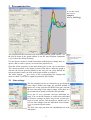
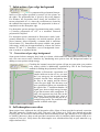
4 Energy calibration
If the absorption spectra are measured in transmission, it is a common practice also to simultaneously
measure the foil. Then the energy axis can be checked for reproducibility and corrected if needed.
If your file format describes the reference curve, you can visualize it or its derivative in this section of
the main dialog. Zoom in the derivative peak, as seen on the screenshots below.
to see this, open the project
Samples/04-ECalib-0.xpj
dots, left Y: μsample
lines, right Y: (μ
(μmetal)'
to see this, open the project
Samples/04-ECalib-1.xpj
Now select the reference en
ergy. If your energy mesh
around the absorption edge is
finely spaced, just use 'maxi
mum of reference curve de
rivative'. In the example
shown the mesh was rough,
0.5 eV. Therefore such a cali
bration will not improve the
energy reproducibility be
tween the two spectra (try it!).
In this case, much better cali
bration is given by manual
positioning of the reference
energy. For this, use 'user-de
fined point' and the pop-up
menu command 'Set reference
energy' (and put it somewhere
close to the peak maximum)
until you merge the reference
curves of all spectra.
dots, left Y: μsample
lines, right Y: (μ
(μmetal)'
Tip: derivative of μ is used when the sample is a foil. In this case you usually do not put the foil also at
the reference position. Then you use the derivative of μ for the sake of energy calibration but not the
derivative of the reference spectrum.
The correcting energy shift is implemented as constant along the spectrum. In contrast to EXAFS,
XANES spectra are short in energy. Therefore the constant energy shift is justified. In EXAFS analy
sis, constant angle and constant lattice shifts are more correct, as implemented in the program VIPER
and explained in its manual.
6
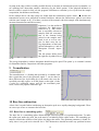
5 Deconvolution of life-time and experimental broadening
See [Klementev 2001] for the description of the Bayesian deconvolution. This procedure is imple
mented in VIPER and XANES dactyloscope.
One can do several deconvolutions one after another (the check box 'apply to initial spectrum' must be
off for this). This makes sense when one first does 'instrumental' and then 'lifetime' deconvolution. The
former is typically of Gaussian kernel and is applied to the measured signals i0 and i1 separately. The
latter is typically of Lorentzian kernel and is applied to μ(E).
There is a way for how to check the solution: after the deconvolution has been found, the back convo
lution is performed by true integration and the resulting deconvolved-convolved μ (I do not know if it
is better to say "deconvoluted-convoluted") is displayed in the graph.
to see this, use the previously loaded example project Samples/04-ECalib-1.xpj
Here on the left there are
two repetitions (red and
blue) of the same spectrum.
On the right the blue one is
deconvolved with the pa
rameters shown above (in
strumental broadening with
ΔE=3.7eV FWHM). The
brown curve is the solution
check,
i.e.
decon
volved-convolved μ. It co
incides with the red one,
which justifies the decon
volution.
You can see this also if you
unselect the deconvolution
made: the initial μ and the
solution check must super
impose.
The Bayesian deconvolution depends on a parameter (regularizer), denoted as α. When it is small, the
solution has rich fine structure, when it is big, the solution is smooth. You can change α and see that
very different deconvolution solutions give successful solution checks. There is no unique solution!
5.1 How to select the regularizer?
One may try to define an optimal, in some sense, α. In [Klementev 2001] I proposed three possible
ways for this. Unfortunately, what I did wrong, I did not consider the spectrum length scaling. For a
full-length spectrum the optimal α must be the same as for its shorter piece. The third method does not
fulfill this. It seems that the second method (the conservation of S/N ratio) is reasonable. The figures of
merit introduced in [Klementev 2001] are reported in XD at the bottom of the deconvolution section of
the main dialog. One can utilize them for (non-automatized) search for an optimum α.
6 Transformation to new grid
In several cases you need to transform your spectra to a common energy grid. For
instance, you need this for Principal component analysis (PCA) or for averaging.
7
7 Subtraction of pre-edge background
The pre-edge background is constructed by polynomial interpo
lation over the region specified by mouse (see the picture on
the right). The polynomial law is given by the power buttons.
For instance, the screenshot above shows the modified Vic
toreen polynomial aE-3+b, where the coefficients are found by
the standard least-squares method. The polynomial is then ex
trapolated over the absorption edge.
For absorption spectra measured in transmission mode, usually
a Victoreen polynomial aE-3+bE-4 or a modified Victoreen
polynomial is implied.
For absorption spectra measured in fluorescence mode, back
ground subtraction is frequently not needed (unselect all the
power buttons). More frequently a constant shift is sufficient
(select button "0"). Sometimes the spectra exhibit a net growth
with energy, which can be approximated by a linear law (select
buttons "0" and "1"). Sometimes a severe background correc
tion is needed, as explained below.
7.1 Corrections of pre-edge background
Some spectra behave strangely: they bend up or down, which makes the background subtraction diffi
cult. One can correct such a behavior by introducing more powers into the background and/or by
adding an extra point at a high energy.
Checking the 'manual correction' option will put an extra point (you position
it by mouse) which is additionally considered by XD in the least-squares
method for finding the polynomial coefficients.
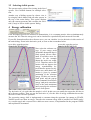
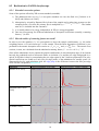
Consider a fluorescence experiment on a
sample inside an in-situ cell. As you scan
the x-ray energy up, the air paths and the
windows become more transparent, thus
the flux at the sample and the fluores
cence flux grow high. This becomes even
more pronounced when you normalize by
the signal of the 1st ionization chamber: its
signal goes down at high energy because
its gas also becomes more transparent. Fi
nally, the spectrum may look like on the
left picture. For correcting this, select at
least 3 polynomial powers and put an ex
tra high energy point. The result after sub
traction is shown at the right.
8 Self-absorption correction
Many papers have addressed the self-absorption effect. Most of them provided restricted correction.
The early papers by [Goulon et al. 1982; Tan et al. 1989; Tröger et al. 1992] were limited only to the
EXAFS case. The correction functions there had discontinuity at the edge and thus were not applicable
to XANES. Moreover, those works provided corrections only for infinitely thick samples with an ex
ception of [Tan et al. 1989] where also thin samples were considered but only as pure materials (e.g.
single element foils).
8
The first self-absorption correction for the whole absorption spectra (also including XANES) was pro
posed with two different strategies by Eisebitt et al. [1993] and Iida and Noma [1993]. Eisebitt et al.
[1993] estimated the two unknowns μtot and μX (see the notations below) from two independent fluores
cence measurements with different positioning of the sample relative to the primary and fluorescence
beams. An obvious disadvantage of this method is that it is solely applicable to polarization-indepen
dent structures (amorphous or of cubic symmetry). On the other hand, it does not require any theoreti
cal tabulation, which is the case in the method of Iida and Noma [1993], who proposed the background
part μback = μtot - μX, to be taken as tabulated. The advantage of their approach is its applicability to any
sample with only one measurement. Moreover, this method is applicable to samples of general thick
ness, not only to thick samples as required by the method of Eisebitt et al. [1993]. It is the method of
Iida and Noma [1993] which is implemented, with some variations, in XD. The method was re-in
vented (i.e. published without citing Iida and Noma [1993]) by Pompa et al. [1995], Haskel [1999] and
Carboni et al. [2005]. These three works, however, were simplified down to infinitely thick limit.
The correction was extended somewhat by considering a variable escape angle in order to account for
the finite (not infinitely small) detector area: only in the synchrotron orbit plane, in EXAFS [Brewe et
al. 1994] and also out of plane: in EXAFS [Pfalzer et al. 1999] and XANES [Carboni et al. 2005]. All
three works operated in the thick limit. To my believe, detector pixels are always small in the sense
that the self-absorption effect can be considered as uniform over each single pixel and therefore the
correction can be done only for one direction towards the pixel center.
An interesting approach to correcting the self-absorption effect was proposed by Booth and Bridges
[2005] who considered another small parameter, not the usual exp(μd), which allowed simplifying
the formulas also beyond the thick limit but the treatment was limited to EXAFS.
Another re-invention of the Iida and Noma method with calling it “new” was presented by Ablett et al.
[2005]. The merit of that work was implementing the method without restriction to the thick limit and
providing many application examples and literature references.
8.1 Description of self-absorption correction
The derivation of the fluorescence intensity can be found, with different notations, in almost all the pa
pers cited above. Here it is repeated because XD adds some extra factors. The standard expression for
the fluorescence intensity originated form the layer dz at the depth z is given by the trivial sequence of
propagation and absorption (with neglected scattering):
dz
sin
dI f z , E= I0
e− E z / sin X E
T
primary primary x-ray
transmitted to
flux
depth z
f
e− E z /sin cos
4 fluorescence x-ray
T
f
transformed
absorbed in layer dz into
directed into transmitted to detector
due to edge of interest fluorescence solid angle from depth z
where μT is the total linear absorption coefficient at the primary x-ray energy
E or the fluorescence energy Ef, μX is the contribution from the edge of inter
est, f is the fluorescence quantum yield – the probability to create a fluores
cence photon from an absorbed photon. After integration over z from 0 to d:
I f E =C
X E
1−e− E d /sin e− E d / sin cos
T
T
f
, (*)
sin
sin cos
where the constant C includes all the energy independent factors and is treated as unknown because the
actual solid angle is usually unknown and also because it implicitly includes the detector efficiency.
T E T E f
The total absorption coefficient is decomposed as T = X b , where the background absorption co
efficient μb is due to all other atoms and other edges of the element of interest. The constant C is found
by equalizing all μ's at a selected energy Enorm (“normalization energy”) to the tabulated ones. Now the
equation (*) can be solved for μX at every energy point E, which is the final goal of the self-absorption
correction.
When the sample is thick (d→∞), the exponent factors vanish. This “thick limit” approximation allows
finding the μX by simple inversion of (*), without solving the non-linear equation, and is optional in XD.
9
8.2 Realization in XANES dactyloscope
8.2.1 Extended correction options
Some of the options offered by XD are non-standard (extended):
1) The additional term cosτ in (*) is not quite standard; one can also find it in [Carboni et al.
2005] and [Ablett et al. 2005].
2) Absorption by air and by Kapton foils in front of the sample can be taken into account (see the
examples below). For this, the primary flux is multiplied by e− E d e− E d . The similar
term at Ef is included into the constant C.
air
air
Kapton
Kapton
3) μb is usually taken to be energy independent. In XD it is energy dependent.
4) One can select among five different tabulations of absorption coefficients (actually, scattering
factors f '') in XD.
8.2.2 How the tables of scattering factors are used?
In order to use the equation (*), it is prerequisite to know the sample stoichiometry, i.e. the molar
weighting factors xi for each atom type i in the sample. Then the linear absorption coefficient is pro
portional to the atomic absorption cross section σa: X ∝ x X aX and T ∝ ∑i x i ai . The atomic cross
sections, in turn, are calculated from the tabulated scattering factors f '': a =2 r 0 ch N A f ' ' /E .
Since all the tabulations do not contain the partial contributions of each absorption edge of an element
but only the combined result of all atomic shells, an isolation of μX and the pre-edge background is re
quired. In XD this is done by extrapolating the pre-edge region by the Victoreen polynomial. The poly
nomial coefficients are found over only two pre-edge points, as the tabulations are usually sparse. As
illustrated below for each tabulation used, the edge jump is the difference between the first post-edge
value and the extrapolated background:
tabulation
Zoomed around the Fe K-edge
[Henke et al. 1993]
[Brennan and Cowan
1992]
[Chantler 1995]
10
Full view of Fe f '' factor [1/atom]
XCOM [Hubbell 1977]
[McMaster et al. 1969]
XD searches for an absorption edge (where the derivative is positive) within –250 eV from the specified
normalization energy. When an edge is found, the jump in molar cross section is displayed in XD.
8.3 Examples
Load the example project Samples/08-fe2o3_tr_fl.xpj. It has 4 spectra of Fe2O3 (hematite) measured in
transmission and fluorescence, each repeated twice to assure reproducibility. The sample is a 13-mmdiameter pressed pellet containing 11 mg of hematite mixed with 80 mg of polyethylene (PE) powder.
The pellet was wrapped by adhesive Kapton foil.
As seen on the left picture,
the fluorescence spectra (red
and green, overlapped) es
sentially differ from the
transmission ones (light and
dark blue, overlapped). As
seen at the right, one of the
two fluorescence spectra
(green) is successfully cor
rected. Notice the EXAFS
amplitude and the pre-edge
peak.
The parameters for the selfabsorption correction are
seen in the screenshot below.
It is essential to remember
about the sample matrix or
the supporting agent (here:
PE) and to put its chemical
formula as well. Here, the
weight '83' of PE (CH2) was
calculated as
mPEMFe2O3 / mFe2O3MPE = 80mg160g/mol / 11mg14g/mol = 83.
In order to use equation (*) for thin samples, one must pro
vide the sample thickness. This could be the physical thick
ness; then one would need to know the sample density for
calculating the linear absorption coefficient in the exponent.
A more direct way is to use the optical thickness μTd, or just
11
its jump at the edge, which is usually possible directly to measure in transmission spectra (remember, we
are speaking here about thin samples, otherwise use the 'thick' option). If the physical thickness is
known, which is usual for foils, use the program XAFSmass to calculate μTd or ΔμXd from the sample
composition, the thickness and density.
In the example above, the edge jump was found from the transmission spectra times 2 because the
transmission spectra were measured at normal incidence whereas the fluorescence spectra were taken
with the same sample at 45º. [For future versions of the manual: redo this example with simultaneously
measured transmission and fluorescence]
Equation (*) is also useful for
correcting the high-energy
behavior of μ. This correc
tion is especially relevant to
samples with low concentra
tion of the element being
probed or the samples mea
sured in air or at low ener
gies. In these cases the en
ergy dependence of the back
ground absorption μb and air
absorption become impor
tant.
The left picture differs from
the right one by added 20 cm
of air.
The energy dependent μb and air absorption should always be opted. The option 'μb is constant' is meant
for illustration and for comparison with other programs.
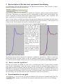
9 Normalization
The normalization, i.e. dividing the spectrum by a constant such
that a particular part of the spectrum equals 1, can be done in
three different ways: by dividing by (i) the mean value over the
specified post-edge region, as on the picture at the right, (ii) the
μ value at a particular energy and (iii) the maximum peak
value, which was popular some time ago.
10 Base line subtraction
A base line is needed when considering an absorption peak on a rapidly changing background. There
are two ways of how to construct the base line.
10.1 Base line as smoothing spline
The base line is a smoothing spline drawn through selected regions of experimental points. To make
the spline pass under the peak, the peak must be excluded from the spline nodes. The smoothing pa
rameter controls the stiffness of the spline: the bigger the stiffer. The optimum parameter is found vis
ually; there is no good strict criterion for it. This arbitrariness should not make any problem because
12
normally the smoothing parameter is (visually) good in a very broad range.
to see this example, load the project Samples/10.1-moallyl-sm-spline.xpj
After subtracting the base line with the
check box 'subtract', the peak is isolated
and can be analyzed for its maximum position (activate the de
rivative for this), total weight (do integration) or peak fitting.
10.2 Base line as spline through adjustable knots
The base line is a spline drawn through the manually put knots.
The knot positions can be adjusted by mouse. The knots may be
constrained to move only along the μ curve (declare them as
'beads') to facilitate the manual set up.
This method can produce more sophisticated shapes of base lines
than the smoothing spline method but requires more time for set
ting it up.
to see the example at the left, load the project
Samples/10.2-moallyl-knots.xpj
After subtraction:
13
11 Factor analysis
11.1 Principal component analysis (PCA)
PCA was described by many authors. In the XAFS community the mostly cited papers seem to be by
Wasserman [1997] (which followed Malinowski [1977]) and by Ressler et al. [2000]. In all the deriva
tions known to me there are two major drawbacks:
1) The PCA test spectra are compared with the data just 'by eye', without statistical grounds for the
comparison. Therefore one cannot say how strongly the PCA mismatch may differ from the experi
mental noise. In other words, not only the mean value is needed for the estimation of noise but also the
confidence limits.
2) The experimental errors of different spectra may obviously differ. For instance, reference materials
usually have much cleaner spectra than typical diluted samples. Therefore the comparison to noise (or,
inversely, the estimation of noise) should be done individually for each spectrum, whereas the standard
derivations concern only the global noise.
The original derivation proposed here is free from the above mentioned drawbacks.
Those of you who, like Winnie-the-Pooh are bothered by long words (formulas), go directly to the
practical description, Section 11.1.3.
11.1.1 Notation and basic facts
Here, capital letters denote matrices, bold italic letters denote vectors (columns). Notice that aT b (in
ner product) is a scalar whereas a b T (outer product) is a matrix.
A symmetric matrix is fully determined by its eigenvalues and eigenvectors: A=∑ j j e j e Tj .
The eigenvectors are orthonormal: eTi e j =ij. Additionally and less trivially: ∑ j e j e Tj =1 (unity matrix).
11.1.2 Derivation of PCA based on statistics
From c measured spectra of length r we form an rc data matrix D=[ d 1 d 2 d c ].
For the covariance matrix DT D find eigenvalues λj and eigenvectors ej and sort them in descending or
der in λ's (λ1 is the largest).
Holds always: ∑cj e j e Tj =1.
If only M<c data vectors are linearly independent, this sum can be truncated at j=M and still
∑Mj e j eTj =1 . In this case λ j ≪ λ1 j>M.
In practice the sum is truncated until D PCA =def D ∑Mj e j eTj coincides with D within noise or, alterna
tively, the truncated part D ∑cj=M 1 e j eTj remains within noise.
How to compare with noise? Denote the PCA residual =D− DPCA , which must be compared with
noise of our data matrix D. Consider
T
T
M
T
T
M
T
c
T
T =1−∑M
k e k e k D D 1−∑ j e j e j =D D−∑ j j e j e j =∑ j=M 1 j e j e j
We are interested in knowing d i−d i PCA 2 for each spectrum di:
d i−d i PCA 2= T ii =∑cj =M 1 j e ji 2 , where eji is the i-th component of eigenvector ej.
On the other hand d i−d i PCA 2 / 2i = i2 if we assume that di PCA reproduces di within noise i (individual
noise of spectrum di). The variate 2i must follow the 2 distribution law with =r c−M /c degrees
of freedom. The scaling factor c−M / c is due to the fact that d i−d i PCA 2 is given by c−M out of
c components. Finally, for the squared noise of spectrum di one gets the mean value
〈 i2 〉= d i −d i PCA 2 /=∑cj=M 1 j e ji 2 / .
14
The confidence limits imin and imax are given by the 2 distribution law at selected significance
levels. In XANES dactyloscope the significance levels are selected to be 2.5% and 97.5% as to give
95% probability that the measurement noise falls within [ imin , imax ] if M out of c spectra are lin
early independent.
One can find the global noise by averaging 〈 i2 〉 over all i:
〈 2 〉=∑cj= M 1 j / c,
where the normality of eigenvectors was used (∑ci e ji 2=1). The last expression is exactly the 'real er
ror' RE introduced by Malinowski [1977]. However, in our derivation we can additionally specify the
confidence limits min and max in the same way as for the individual noise i i.e. by using the statistical
properties of 2 distribution.
11.1.3 Questions answered by PCA
Unlike the usual descriptions of PCA, the derivation proposed here is capable of answering two direct
and two inverse questions:
PCA1) Given the global (average) noise level, how many spectra are linearly independent?
PCA1') How high must be the global noise level in order to have a given number of independent spectra?
PCA2) Given the noise level of a particular spectrum, how many principal components are needed to
reproduce the spectrum?
PCA2') How high must be the noise level of a particular spectrum in order to reproduce it by a speci
fied number of principal components?
As you will see in the example in Section 11.1.6 below, the questions PCA1 and PCA2 are not quite
the same.
In order to answer the direct questions PCA1 and PCA2 you must know the experimental noise level.
How to determine it? See Section 13.
11.1.4 How the PCA results are related to chemical species?
A mechanical mixture of chemical species obviously results in a linear combination of the correspond
ing spectra. However, if different species have similar XANES spectra, the spectra may be linearly de
pendent even for a set of pure chemical species. The example in Section 11.3.1 illustrates this case.
Note therefore that linear dependence of spectra does not necessarily mean mixture of species!
Inversely, if some spectra are distorted due to self-absorption, non-linearity of the fluorescence detec
tor, presence of pin holes etc., linear dependence of spectra may be lost although the samples may re
ally represent mixtures.
Finally, this question should be individually explored in every PCA study. It also involves careful at
tention to experimental details in order to eliminate systematic distortions.
11.1.5 Is PCA also applicable to EXAFS?
Formally yes, and some people did it, but with very poor logic. EXAFS is described by a sum of modu
lated sinus functions. Sinus functions form a complete set and as such can be linearly combined to repro
duce any function. Thus it is naturally expected that EXAFS spectra are linearly dependent. The 'bad' na
ture of the EXAFS kernel can also be seen from another side: it is impossible, if without any regulariza
tion scheme, to invert the EXAFS equation for getting the radial distribution function. The reason is the
same: the degeneracy of the kernel i.e. its low rank when expressed as a matrix of (2k, r) coordinates.
Finally, the functional shape of EXAFS makes one EXAFS spectrum strongly correlate with another
one. This correlation happens regardless of spatial structural correlations. Doing conclusions on PCA ap
plied to EXAFS spectra does not substantiate any conclusions on the number of independent structures.
Yet finally, don't do PCA on EXAFS!
15
11.1.6 Usage of PCA in XANES dactyloscope
The spectra subject to PCA or target transformation must be defined on the same energy grid. If the
grids are different, do the transform (Section 6).
Specify a set of spectra. This is considered either as a data set or as a basis set depending on whether
the current spectrum belongs to it. Then, correspondingly, PCA or target transformation is performed.
Load the project Samples/11.1-PCA2-dABCnC.xpj which has
two independent spectra and a spectrum constructed as the aver
age of the two plus normal noise with nominal σ = 0.005. The
thick curves are data and the thin blue ones are the PCA-test
curves. The components can be selected/unselected by pressing
the button 'principal components'. Unselecting a component
means excluding it from the principal ones. As seen, the test
curves reproduce the data exactly when all the components are
selected.
Unselect the last component which is the least important one. As
seen on the picture at the right, the spectra are still well repro
duced, which is expected as we know that there are two indepen
dent spectra and there must be two PC's.
16
Unselect the second compo
nent and see that the first
two spectra are reproduced
badly ('hide all other spectra'
may help in seeing this bet
ter), left picture, whereas the
third one can surprisingly be
reproduced with only one
principal component, right
picture. This fact shows that
some particular spectra may
contain less principal com
ponents than the number of
independent spectra and that
the latter figure may be un
derestimated by visual
checking of PCA test. This
example shows also what is
the first principal component
in this case: it is the average
spectrum.
The figures ' min .. 〈〉 .. max' reported in the pop-up menu under the button 'prin
cipal components' allow to answer the questions listed in Section 11.1.3.
PCA1) Given the global noise level, how many spectra are linearly independent?
The 'global 95% noise bounds' tell that with 95% of probability the measurement
noise must be within the bounds in order to consider the component as unimpor
tant and unselect it from the list of PC's. If your experimental noise is lower then
this component must stay selected, if it is higher then there must be some further
correlations among the selected components and you should unselect yet more
components. Finally, the number of the selected components gives the number of
independent spectra. Of course, you do not have to select/unselect the menu
items. Just look at the values: where the noise estimations are bigger than the ex
perimental noise, these are the principal components.
PCA1') How high must be the global noise level in order to have a given number of independent spectra?
The answer with 95% significance level is in the pop-up menu on one line below the given ordinal
number.
PCA2) Given the noise level of a particular spectrum, how many principal components are needed to
reproduce the spectrum?
for spectrum “1”: The answer, similarly to PCA1, is given by the pop-up menu for spectrum “3”:
but in the section 'individual 95% noise bounds'. Notice that
these figures are reported only for the current spectrum and
generally differ from those for another spectrum, as shown on
the left and right pictures.
PCA2') How high must be the noise level of a particular spectrum in order to reproduce it by a speci
fied number of principal components?
The answer is similar to PCA1' but in the 'individual …' section. The figures refer to the current spectrum.
In the example above, the artificially added normal noise of σ = 0.005 falls within:
(PCA1) the global noise bounds of the third component, which means two principal components;
(PCA2) the individual noise bounds of (a) the second component when the 3 rd spectrum is active,
which means only one component reproducing the 3rd spectrum; (b) the third component when the 1st
or 2nd spectrum is active, which means two components reproducing the 1st and 2nd spectrum.
17
Let us consider another example:
Samples/11.2-PCA8-(dA1+n)10.xpj. It has 10 spectra which are
all artificially constructed from a single spectrum with added 10
various realizations of normal noise of nominal σ = 0.005.
The individual and global noise estimations correctly give only
one principal component and the noise level close to 0.005.
The experimental noise level can be found
from averaging (see Section 13) as
0.0046.
11.2 Target transformation (TT)
You can skip the derivation and go directly to the practical description, Section 11.2.2.
11.2.1 Derivation of TT based on statistics
From c measured basis (reference) spectra of length r we form an rc basis matrix B=[ b1 b 2 b c ] .
If the basis spectra are linearly independent then the covariance matrix B T B is of rank c and then
BT B−1 exists.
The matrix B BT B−1 BT is an orthogonal projector to the basis space since it is equal to its square:
B BT B−1 B T 2=B BT B−1 B T B BT B−1 BT =B BT B−1 BT .
Hence, if a spectrum d is a linear combination of the basis spectra then
B BT B−1 BT d =d and vice versa.
In practice one checks if B BT B−1 BT d coincides with d within noise. The inverse matrix BT B−1 is
found through the eigenvalues and eigenvectors of B T B as
T
BT B−1=∑ j −1
j ejej.
This allows to simultaneously do PCA on the basis set in order to check that the basis spectra are inde
pendent.
Denote the TT residual =d −B BT B−1 BT d , which must be compared with noise of our spectrum d.
Taking into account the projector property of B BT B−1 BT , we get
T =d T 1−B B T B−1 BT 1−B BT B−1 B T d =d T 1−B BT B−1 BT d .
On the other hand, we represent the spectrum d by a direct sum of the basis spectra B plus a contribu
tion n orthogonal to B:
d= B bn ,
where b is a c-dimensional vector representing the weights of the c basis spectra. Because
1−B BT B−1 BT B b=B b−B b=0 ,
18
and because of orthogonality of n to B, it follows that
T =nT n .
Finally, if n is solely due to noise , the variate 2= T / 2 must follow the 2 distribution law with
=r −c degrees of freedom. Thus the mean value of the squared noise is
〈 2 〉= T / .
The confidence limits min and max are found in the same way as in PCA, i.e. by using the statistical
properties of 2 distribution.
Notice that we cannot use the target transformation method to determine the decomposition weights b
because the expression for the experimental squared target transformation residual T does not con
tain b! On the contrary, the squared linear fitting residual d −∑ B b2 does contain b whence it can be
determined.
11.2.2 Questions answered by TT
One direct and one inverse question:
TT1) Given the noise level of a particular spectrum, can the spectrum be reproduced by a linear combi
nation of the basis spectra?
TT1') How high must be the noise level of a particular spectrum in order to reproduce it by a linear
combination of the basis spectra?
11.2.3 Usage of TT in XANES dactyloscope
To perform TT of a spectrum, specify a basis set which does not include the target transformed spec
trum (the current spectrum).
Note that in TT all the components must be selected. It does not make sense to truncate the sum
T
BT B−1=∑ j −1
j e j e j because the basis spectra are supposed to be linearly independent.
Again load the project Samples/11.1-PCA2-dABCnC.xpj which
has two independent spectra and a spectrum constructed as the
average of the two plus normal noise with σ = 0.005. For the 3 rd
spectrum active, specify the basis set as '1,2' and see the resulting
figures under the button 'target tracking'.
The experimental noise of the target
transformed spectrum (here, σ = 0.005)
must be within the given noise bounds
for the question TT1 be answered posi
tively. If the experimental noise is
smaller then there are important contri
butions which are not inside the basis
set. If it is larger (which is unusual)
then there are some extra correlations between the basis spectra
and the target transformed spectrum, e.g. it is artificially con
structed by a linear combination of the basis spectra including
their noise.
Check also that the noise estimation of the last principle compo
nent of the basis set (here, 0.07393) is much higher than the ex
perimental noise, otherwise the basis set is bad, i.e. internally lin
early dependent.
19
11.3 Pitfalls in factor analysis
11.3.1 Overestimated linear dependence
If different species have similar XANES spectra, the spectra may be linearly dependent even for a set
of pure chemical species. To illustrate this, load the project Samples/11.3-PCA-MoOx.xpj which has
spectra of 6 molybdenum oxides: MoO2, Mo14O11, Mo5O14, Mo8O23, Mo18O52 and MoO3. [J. Wienold,
T. Ressler, private communication; Ressler et al. 2002]. As seen, there are only 4 or 5 independent
spectra out of 6 although each sample has a pure structure as was proven by XRD.
Another example of overestimated linear dependence is given by PCA applied to EXAFS (see Section
11.1.5). EXAFS spectra are usually more linearly dependent than the corresponding spatial structures.
11.3.2 Underestimated linear dependence
Always remember that spectra may have instrumental distortions due to self-absorption, non-linearity
of the fluorescence detector, presence of pin holes etc. These distortions may break the linear depen
dence of spectra even where it would be really expected.
Consider an example of self-absorption from Section 8.3. Load the example project Samples/08fe2o3_tr_fl.xpj. It has 4 spectra of Fe2O3 (hematite): measured in transmission and fluorescence, each
repeated twice to assure reproducibility. To enable PCA, transform the energy mesh to a new grid
with, e.g. 1st node 7080 eV and dE=0.5 eV. Apply this transform to all 4 spectra. Switch off the selfabsorption correction and activate PCA. As seen in the list of PC's, there are two components with low
estimated noise and, hence, there are two PC's, as expected. Now switch on the self-absorption correc
tion again and see that the 3rd component in PCA has quite high noise estimation which does not let ne
glect it. In other words, the corrected spectrum represents an “independent” species which does not
fully merge with the transmission spectra. Inversely, this noise estimation can be taken as the noise
level used instead of the experimental noise in the PCA's involving the self-absorption corrected fluo
rescence spectra of hematite.
In summarizing this example, concentrated references measured in fluorescence must be corrected for
self-absorption. Even being corrected, the fluorescence spectra may significantly differ from the trans
mission ones and thus introduce “new” species into the set of principle components.
11.4 Recommendations for factor analysis
•
The reference compounds, as they normally are concentrated, are better to measure in transmis
sion in order to reduce the added uncertainty due to the self-absorption correction.
•
All amplitude distortions must be well understood and prevented/corrected.
•
It always makes sense measuring a calibrated test mixture.
12 Fitting by user-defined formula
The primary usage of this section is doing a linear combination fitting after the factor analysis.
The fitting formula is typed in by the user. It operates the letters 'a' through 'y' ('E' stands for energy as
independent variable; it is internally renamed to 'z') and 'any' usual mathematical operations and func
tions. A letter can be declared as a fitting parameter or a spectrum loaded by XD. In the latter case its
energy shift may vary as an additional fitting parameter. This capability can be useful when the energy
axis is not well reproducible or when mixing data from various beamlines or, as in the example below,
when modeling different spectral features by a single contribution.
Load the project Samples/12-cefit34.xpj which has a Ce L3 XANES (spectrum #2, red) fitted by a
weighted sum of monovalent 3+ and 4+ contributions. The "3+" spectrum was calculated by FEFF
(spectrum #1, black). The "4+" contribution is represented by the same calculated spectrum shifted by
a fitting value to higher energies.
20
Thus the experimental spectrum is fitted by the formula 'a+b*c',
where 'a' and 'b' are the same shifted spectrum #1 (the black
curve), 'c' is a scalar:
The average valence is given in this case by [(3+)+(4+)·c]/(1+c).
After the automatic fitting has finished, press 'Statistics...' button.
You should select the 'integrated' option for the errors (δ's) of the
fitting parameters. See VIPER manual for the description of the
other options and the methods behind. See VIPER manual for the
description of the statistical χ2 and F-tests.
The colored matrix shows the pair-correlation coefficients. Com
pletely red and blue denote +1 and 1, black is 0. The fitting er
rors are listed at the left of the correlation matrix. Pay attention to
the correlation coefficients. They should not be close to +1 or 1
or, visually, much colored or, when displayed by the correlation
map (the yellow-black graph), diagonally stretched. This would
mean large fitting errors and frustration for the minimization al
gorithm. In this case try to apply constraints to the fitting param
eters using the button 'Constrain...'. Alternatively, one can fix a
fitting parameter by setting its initial increment to zero.
13 Creating average, rms and difference spectra
Average, rms and difference spectra can be added via 'Spectra' menu:
Such spectra, called 'special' in XD, are updated whenever the original
spectra from which the special spectra were constructed have changed.
Here you can average several repetitions of one spectrum and/or sev
eral fluorescence spectra measured by a multi-pixel detector.
An rms spectrum is useful for determining the experimental noise.
Load the project: Samples/11.2-PCA8-(dA1+n)10.xpj. It has 10 spec
tra which are all artificially constructed from a single spectrum with
added 10 various realizations of normal noise of nominal σ = 0.005. Cre
ate an rms spectrum and make it active. In the description line at the top
of the main dialog window find the mean value of the rms spectrum. This value can further be used in
factor analysis or in calculating the fitting errors.
21
14 Exporting data and saving project file
The curves visible in the main graph window can be ex
ported to a column file, use 'Project/Make output file...'.
Another very useful function of XD is saving project files.
A project file has description of data files and all the pro
cessing steps. The project files Samples/*.xpj have been
saved in this way.
Important: Project files are text file. You can edit them
by any common editor. A newly created project file has
full path references to the data files. If you move the data
files or if you want to load the project on another com
puter, you should change the paths accordingly. I nor
mally keep project files in the same directory with data.
Then I keep only the file names in a project file and manu
ally delete the directory paths by Search/Replace com
mand in a text editor.
References
Ablett J M, Woicik J C and Kao C C (2005) International Centre for Diffraction Data, Advances in Xray Analysis 48, 266.
Booth C H and Bridges F (2005) Physica Scripta T115, 202.
Brennan S and Cowan P L (1992) Rev. Sci. Instrum. 63, 850
http://www.bmsc.washington.edu/scatter/periodic-table.html
ftp://ftpa.aps.anl.gov/pub/cross-section_codes/
Brewe D L, Pease D M and Budnick J I (1994) Phys. Rev. B 50, 9025.
Carboni R, Giovannini S, Antonioli G and Boscherini F (2005) Physica Scripta T115, 986.
Chantler C T (1995) J. Phys. Chem. Ref. Data 24, 71
http://physics.nist.gov/PhysRefData/FFast/Text/cover.html
http://physics.nist.gov/PhysRefData/FFast/html/form.html
Eisebitt S, Böske T, Rubensson J-E and Eberhardt W (1993) Phys. Rev. B 47, 14103.
Goulon J, Goulon-Ginet C, Cortes R and Dubois J M (1982) J. Physique 43, 539.
Haskel D (1999) Computer program FLUO: Correcting XANES for self absorption in fluorescence
data, http://www.aps.anl.gov/xfd/people/haskel/fluo.html .
Henke B L, Gullikson E M and Davis J C (1993) Atomic Data and Nuclear Data Tables 54, 181.
http://www-cxro.lbl.gov/optical_constants/
Hubbell J H (1969) Natl. Stand. Ref. Data Ser. 29; Hubbell J H, Radiat. Res. 70 (1977) 58-81.
http://physics.nist.gov/PhysRefData/Xcom/Text/XCOM.html
Iida A and Noma T (1993) Jpn. J. Appl. Phys. 32, 2899.
Kissel L, Zhou B, Roy S C, Sen Gupta S K and Pratt R H (1995) Acta Crystallographica A51, 271;
Pratt R H, Kissel L and Bergstrom Jr. P M, New Relativistic S-Matrix Results for Scattering - Beyond
the Usual Anomalous Factors/ Beyond Impulse Approximation, in Resonant Anomalous X-Ray Scat
tering, edited by G. Materlik, C. J. Sparks and K. Fischer (North-Holland: Amsterdam, 1994); Kane P
P, Kissel L, Pratt R H and Roy S C Physics Reports 140, 75-159 (1986); Kissel L and Pratt R H,
Rayleigh Scattering - Elastic Photon Scattering by Bound Electrons, in Atomic Inner-Shell Physics,
edited by Bernd Crasemann (Plenum Publishing: New York, 1985).
http://www-phys.llnl.gov/Research/scattering/index.html
Klementev K V (2001) J. Phys. D: Appl. Phys. 34, 2241.
22
Malinowski Edmund R (1977) Anal. Chem. 49, 606.
McMaster W H, Kerr Del Grande N, Mallett J H and Hubbell J H (1969) Compilation of X-Ray Cross
Sections Lawrence Livermore National Laboratory Report UCRL-50174 Section II Revision I avail
able from National Technical Information Services L-3, U.S. Dept. of Commerce
http://ixs.csrri.iit.edu/database/programs/mcmaster.html
http://cars9.uchicago.edu/~newville/mcbook/
Pfalzer P, Urbach J-P, Klemm M, Horn S, denBoer M L, Frenkel A I and Kirkland J P (1999) Phys.
Rev. B 60, 9335.
Pompa M, Flank A-M, Delaunay R, Bianconi A and Lagarde P (1995) Physica B 208&209, 143.
Ressler T, Wong J, Roos J and Smith I L (2000) Env. Sci. & Technol. 34, 950 .
Ressler T, Wienold J, Jentoft R E and Neisius T (2002) J. of Catalysis 210, 67.
Tan Z, Budnick J I and Heald S M (1989) Rev. Sci. Instrum. 60, 1021.
Tröger L, Arvanitis D, Baberschke K, Michaelis H, Grimm U and Zschech E (1992) Phys. Rev. B 46, 3283.
Wasserman S R (1997) J. Phys. IV France 7, C2-203.
23