Download S. Sriram`s Thesis - Electrical Engineering & Computer Sciences

Table of Contents
1
INTRODUCTION............................................................................................1
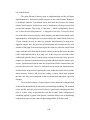
1.1 The Synchronous Dataflow model....................................................7
1.1.1 Background........................................................................7
1.1.2 Utility of dataflow for DSP .............................................11
1.2 Parallel scheduling ..........................................................................13
1.2.1 Fully-static schedules ......................................................15
1.2.2 Self-timed schedules........................................................19
1.2.3 Execution time estimates and static schedules ................21
1.3 Application-specific parallel architectures......................................24
1.3.1 Dataflow DSP architectures ............................................24
1.3.2 Systolic and wavefront arrays .........................................25
1.3.3 Multiprocessor DSP architectures ...................................26
1.4 Thesis overview: our approach and contributions ..........................27
2
TERMINOLOGY AND NOTATIONS ........................................................33
2.1 HSDF graphs and associated graph theoretic notation ...................33
2.2 Schedule notation ............................................................................35
3
THE ORDERED TRANSACTION STRATEGY.......................................39
3.1 The Ordered Transactions strategy .................................................39
3.2 Shared bus architecture ...................................................................42
3.2.1 Using the OT approach....................................................46
3.3 Design of an Ordered Memory Access multiprocessor ..................47
3.3.1 High level design description ..........................................48
3.3.2 A modified design ...........................................................49
3.4 Design details of a prototype ..........................................................52
3.4.1 Top level design ..............................................................53
3.4.2 Transaction order controller ............................................55
3.4.2.1. Processor bus arbitration signals......................55
3.4.2.2. A simple implementation .................................57
iii
3.4.2.3. Presettable counter ...........................................58
3.4.3 Host interface...................................................................60
3.4.4 Processing element ..........................................................61
3.4.5 Xilinx circuitry ................................................................62
3.4.5.1. I/O interface .....................................................64
3.4.6 Shared memory................................................................65
3.4.7 Connecting multiple boards.............................................65
3.5 Hardware and software implementation .........................................66
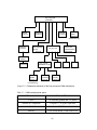
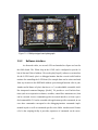
3.5.1 Board design....................................................................66
3.5.2 Software interface............................................................69
3.6 Ordered I/O and parameter control .................................................71
3.7 Application examples......................................................................73
3.7.1 Music synthesis ...............................................................73
3.7.2 QMF filter bank...............................................................75
3.7.3 1024 point complex FFT .................................................76
3.8 Summary .........................................................................................78
4
AN ANALYSIS OF THE OT STRATEGY .................................................79
4.1 Inter-processor Communication graph (Gipc) .................................82
4.2 Execution time estimates ................................................................88
4.3 Ordering constraints viewed as edges added to Gipc .............................89
4.4 Periodicity .......................................................................................90
4.5 Optimal order ..................................................................................92
4.6 Effects of changes in execution times.............................................96
4.6.1 Deterministic case ...........................................................97
4.6.2 Modeling run time variations in execution times ............99
4.6.3 Implications for the OT schedule ..................................104
4.7 Summary .......................................................................................106
5
MINIMIZING SYNCHRONIZATION COSTS IN SELF-TIMED
SCHEDULES ...............................................................................................107
iv
5.1 Related work .................................................................................108
5.2 Analysis of self-timed execution...................................................112
5.2.1 Estimated throughput.....................................................114
5.3 Strongly connected components and buffer size bounds ..............114
5.4 Synchronization model .................................................................116
5.4.1 Synchronization protocols .............................................116
5.4.2 The synchronization graph Gs ..................................................118
5.5 Formal problem statement ............................................................122
5.6 Removing redundant synchronizations .........................................124
5.6.1 The independence of redundant synchronizations ........125
5.6.2 Removing redundant synchronizations .........................126
5.6.3 Comparison with Shaffer’s approach ............................128
5.6.4 An example....................................................................129
5.7 Making the synchronization graph strongly connected ................131
5.7.1 Adding edges to the synchronization graph ..................133
5.7.2 Insertion of delays .........................................................137
5.8 Computing buffer bounds from Gs and Gipc...........................................141
5.9 Resynchronization.........................................................................142
5.10 Summary .......................................................................................144
6
EXTENSIONS..............................................................................................147
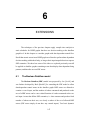
6.1 The Boolean Dataflow model .......................................................147
6.1.1 Scheduling .....................................................................148
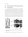
6.2 Parallel implementation on shared memory machines .................152
6.2.1 General strategy.............................................................152
6.2.2 Implementation on the OMA.........................................155
6.2.3 Improved mechanism ....................................................157
6.2.4 Generating the annotated bus access list .......................161
6.3 Data-dependent iteration ...............................................................164
6.4 Summary .......................................................................................165
v
7
CONCLUSIONS AND FUTURE DIRECTIONS.....................................166
8
REFERENCES.............................................................................................170
vi
List of Figures
Figure 1.1.
Fully static schedule ........................................................................ 16
Figure 1.2.
Fully-static schedule on five processors.......................................... 17
Figure 1.3.
Steps in a self-timed scheduling strategy ........................................ 20
Figure 3.1.
One possible transaction order derived from the fully-static schedule
.........................................................................................................41
Figure 3.2.
Block diagram of the OMA prototype ............................................ 49
Figure 3.3.
Modified design............................................................................... 50
Figure 3.4.
Details of the “TA” line mechanism (only one processor is shown) .
.........................................................................................................51
Figure 3.5.
Top-level schematic of the OMA prototype.................................... 54
Figure 3.6.
Using processor bus arbitration signals for controlling bus access. 56
Figure 3.7.
Ordered Transaction Controller implementation ............................ 58
Figure 3.8.
Presettable counter implementation ................................................ 59
Figure 3.9.
Host interface .................................................................................. 61
Figure 3.10. Processing element .......................................................................... 62
Figure 3.11. Xilinx configuration at run time ..................................................... 64
Figure 3.12. Connecting multiple boards ............................................................ 67
Figure 3.13. Schematics hierarchy of the four processor OMA architecture ...... 68
Figure 3.14. OMA prototype board photograph .................................................. 69
Figure 3.15. Steps required for downloading code (tcl script omaDoAll)........... 70
Figure 3.16. Hierarchical specification of the Karplus-Strong algorithm in 28
voices............................................................................................... 74
Figure 3.17. Four processor schedule for the Karplus-Strong algorithm in 28
voices. Three processors are assigned 8 voices each, the fourth (Proc
1) is assigned 4 voices along with the noise source. ....................... 75
Figure 3.18. (a) Hierarchical block diagram for a 15 band analysis and synthesis
filter bank. (b) Schedule on four processors (using Sih’s DL heuristic
[Sih90])............................................................................................ 77
vii
Figure 3.19. Schedule for the FFT example. ....................................................... 78
Figure 4.1.
Fully-static schedule on five processors.......................................... 80
Figure 4.2.
Self-timed schedule ......................................................................... 81
Figure 4.3.
Schedule evolution when the transaction order of Fig. 3.1 is
enforced ........................................................................................... 81
Figure 4.4.
The IPC graph for the schedule in Fig. 4.1. .................................... 83
Figure 4.5.
Transaction ordering constraints ..................................................... 89
Figure 4.6.
Modified schedule S´ ....................................................................... 95
Figure 4.7.
Gipc, actor C has execution time tc, constant over all invocations of C
....................................................................................................................97
Figure 4.8.
TST(tC) ....................................................................................................... 98
Figure 4.9.
Gipc with transaction ordering constraints represented as dashed lines
.......................................................................................................105
Figure 4.10. TST(tC) and TOT(tC)................................................................................. 105
Figure 5.1.
(a) An HSDFG (b) A three-pro(a) An HSDFG (b) A three-processor
self-timed schedule for (a). (c) An illustration of execution under the
placement of barriers. .................................................................... 110
Figure 5.2.
Self-timed execution ..................................................................... 113
Figure 5.3.
An IPC graph with a feedforward edge: (a) original graph (b) imposing bounded buffers....................................................................... 115
Figure 5.4.
x2 is an example of a redundant synchronization edge. ................ 124
Figure 5.5.
An algorithm that optimally removes redundant synchronization
edges.............................................................................................. 127
Figure 5.6.
(a) A multi-resolution QMF filter bank used to illustrate the benefits
of removing redundant synchronizations. (b) The precedence graph
for (a). (c) A self-timed, two-processor, parallel schedule for (a). (d)
The initial synchronization graph for (c)....................................... 130
Figure 5.7.
The synchronization graph of Fig. 5.6(d) after all redundant synchronization edges are removed. .......................................................... 132
Figure 5.8.
An algorithm for converting a synchronization graph that is not
vii
strongly connected into a strongly connected graph. .................... 133
Figure 5.9.
An illustration of a possible solution obtained by algorithm Convertto-SC-graph. .................................................................................. 134
Figure 5.10. The synchronization graph, after redundant synchronization edges
are removed, induced by a four-processor schedule of a music synthesizer based on the Karplus-Strong algorithm. .......................... 136
Figure 5.11. A possible solution obtained by applying Convert-to-SC-graph to the
example of Figure 5.10.................................................................. 137
Figure 5.13. An example used to illustrate a solution obtained by algorithm DetermineDelays.................................................................................... 138
Figure 5.12. An algorithm for determining the delays on the edges introduced by
algorithm Convert-to-SC-graph. ................................................... 139
Figure 5.14. An example of resynchronization. ................................................ 143
Figure 5.15. The complete synchronization optimization algorithm................. 145
Figure 6.1.
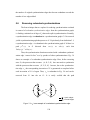
BDF actors SWITCH and SELECT.............................................. 148
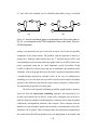
Figure 6.2.
(a) Conditional (if-then-else) dataflow graph. The branch outcome is
determined at run time by actor B. (b) Graph representing datadependent iteration. The termination condition for the loop is determined by actor D. .......................................................................... 149
Figure 6.3.
Acyclic precedence graphs corresponding to the if-then-else graph of
Fig. 6.2. (a) corresponds to the TRUE assignment of the control
token, (b) to the FALSE assignment. ............................................ 150
Figure 6.4.
Quasi-static schedule for a conditional construct (adapted from
[Lee88b]) ....................................................................................... 152
Figure 6.5.
Programs on three processors for the quasi-static schedule of Fig.
6.4.................................................................................................. 153
Figure 6.6.
Transaction order corresponding to the TRUE and FALSE branches .
........................................................................................................155
Figure 6.7.
Bus access list that is stored in the schedule RAM for the quasi-static
schedule of Fig. 6.6. Loading operation of the schedule counter conix
ditioned on value of c is also shown.............................................. 157
Figure 6.8.
Conditional constructs in parallel paths ........................................ 158
Figure 6.9.
A bus access mechanism that selectively “masks” bus grants based
on values of control tokens that are evaluated at run time ............ 159
Figure 6.10. Bus access lists and the annotated list corresponding to Fig. 6.6.. 161
Figure 6.11. Quasi-static schedule for the data-dependent iteration graph of Fig.
6.2(b). ............................................................................................ 164
Figure 6.12. A possible access order list corresponding to the quasi-static schedule of Fig. 6.11. ............................................................................. 165
Figure 7.1.
An example of how execution time guarantees can be used to reduce
buffer size bounds. ........................................................................ 168
x
ACKNOWLEDGEMENTS
I have always considered it a privilege to have had the opportunity of pursuing my Ph.D. at Berkeley. The time I have spent here has been very fruitful, and
I have found the interaction with the exceptionally distinguished faculty and the
smart set of colleagues extremely enriching. Although I will not be able to
acknowledge all the people who have directly or indirectly helped me during the
course of my Ph. D., I wish to mention some of the people who have influenced me
most during my years as a graduate student.
First and foremost, I wish to thank Professor Edward Lee, my research
advisor, for his valuable support and guidance, and for having been a constant
source of inspiration for this work. I really admire Professor Lee’s dedication to
his research; I have learned a lot from his approach of conducting research.
I also thank Professors Pravin Varaiya and Henry Helson for serving on my
thesis committee. I thank Professor David Messerschmitt for his advice; I have
learned from him, both in the classroom as well as through his insightful and
humorous “when I was at Bell Labs ...” stories at our Friday afternoon post-seminar get-togethers. I have also greatly enjoyed attending classes and discussions
with Professors Avideh Zakhor, Jean Walrand, John Wawrzynek, and Robert Brayton. I thank Professors Michael Lieberman and Allan Lichtenberg for their support
and encouragement during my first year as a graduate student.
During the course of my Ph. D. research I have had the opportunity to work
closely with several fellow graduate students. In particular I would like to mention
Shuvra Bhattacharyya, in collaboration with whom some of the work in this thesis
was done, and Praveen Murthy. Praveen and Shuvra are also close friends and I
xi
have immensely enjoyed my interactions with them, both technical as well as nontechnical (such as music, photography, tennis, etc.).
I want to thank Phil Lapsley, who helped me with the DSP lab hardware
when I first joined the DSP group; Soonhoi Ha, who helped me with various
aspects of the scheduling implementation in Ptolemy; and Mani Srivastava, who
helped me a great deal with printed circuit board layout tools, and provided me
with several useful tips that helped me design and prototype the 4 processor OMA
board.
I should mention Mary Stewart and Carol Sitea for helping me with reimbursements and other bureaucratic paperwork, Christopher Hylands for patiently
answering my system related queries, and Heather Levien for cheerfully helping
me with the mass of graduate division related paperwork, deadlines, formalities to
be completed, etc.
I have enjoyed many useful discussions with some of some of my friends
and colleagues, in particular Alan Kamas (I have to mention his infectious sense of
humor), Louis Yun, Wan-teh Chan, Rick Han, William Li, Tom Parks, Jose Pino,
Brian Evans, Mike Williamson, Bilung Lee and Asawaree Kalavade, who have
made my (innumerable) hours in Cory Hall much more fun than what would have
been otherwise. I will miss the corridor/elevator discussions (on topics ranging
from the weather to Hindu philosophy) with Sriram Krishnan (the other Sriram),
Jagesh Sanghavi, Rajeev Murgai, Shankar Narayanaswami, SKI, Angela Chuang,
Premal Buch; and so will I miss the discussions, reminiscences and retelling of old
tales with the sizable gang of graduate students in Berkeley and Stanford with
whom I share my alma mater (IIT Kanpur) — Vigyan, Adnan, Kumud, Sunil,
Amit Narayan, Geetanjali, Sanjay, Vineet, Ramesh, to name a few.
While at Berkeley, I have met several people who have since become good
xii
friends: Juergen Teich, Raghuram Devarakonda, Amit Lal, Amit Marathe, Ramesh
Gopalan, Datta Godbole, Satyajit Patwardhan, Aparna Pandey, Amar Kapadia. I
thank them all for their excellent company; I have learned a lot from their talents
and experiences as well.
I also wish to thank my long time friends Anurag, Ashish, Akshay, Anil,
Kumud, Nitin, RD, Sanjiv — our occasional get-togethers and telephone chats
have always provided a welcome relief from the tedium that grad school sometimes tends to become.
Of course, the Berkeley experience in general — the beautiful campus with
great views of the San Francisco bay and the Golden Gate, the excellent library
system, the cafe´s and the restaurants, the CD shops and the used book stores, student groups and cacophonic drummers on Sproul plaza, the Hateman and the
Naked Guy — has left me with indelible memories, and a wealth of interesting stories to tell, and has also helped keep my efforts towards a Ph. D. in perspective.
Finally, I wish to thank my parents for all their support and belief in me,
and my sister, who has a knack for boosting my morale during rough times. I dedicate this thesis to them.
xiii
1
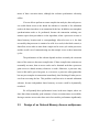
in both these respects: the programmable core needs to be verified for correctness
only once, and design changes can be made late in the design cycle by modifying
the software program. Although verifying the embedded software to be run on a
programmable part is also a hard problem, in most situations changes late in the
design cycle (and indeed even after the system design is completed) are much easier and cheaper to make in the case of software than in the case of hardware.
INTRODUCTION
Special processors are available today that employ an architecture and an
instruction set tailored towards signal processing. Such software programmable
integrated circuits are called “Digital Signal Processors” (DSP chips or DSPs for
short). The special features that these processors employ are discussed by Lee in
[Lee88a]. However, a single processor — even DSPs — often cannot deliver the
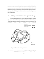
The focus of this thesis is the exploration of architectures and design meth-
performance requirement of some applications. In these cases, use of multiple pro-
odologies for application-specific parallel systems for embedded applications in
cessors is an attractive solution, where both the hardware and the software make
digital signal processing (DSP). The hardware model we consider consists of mul-
use of the application-specific nature of the task to be performed.
tiple programmable processors (possibly heterogeneous) and multiple application-
Over the past few years several companies have been offering boards con-
specific hardware elements. Such a heterogeneous architecture is found in a num-
sisting of multiple DSP chips. More recently, semiconductor companies are offer-
ber of embedded applications today: cellular radios, image processing boards,
ing chips that integrate multiple CPUs on a single die: Texas Instruments (the
music/sound cards, robot control applications, etc. In this thesis we develop sys-
TMS320C80 multi-DSP), Star Semiconductors (SPROC chip), Adaptive Solutions
tematic techniques aimed at reducing inter-processor communication and synchro-
(CNAPS processor), etc. Multiple processor DSPs are becoming popular because
nization costs in such multiprocessors that are designed to be application-specific.
of variety of reasons. First, VLSI technology today enables one to “stamp” 4-5
The techniques presented in this thesis apply to DSP algorithms that involve sim-
standard DSPs onto a single die; this trend is only going to continue in the coming
ple control structure; the precise domain of applicability of these techniques will
years. Such an approach is expected to become increasingly attractive because it
be formally stated shortly.
reduces the testing time for the increasingly complex VLSI systems of the future.
Applications in signal processing and image processing require large com-
Second, since such a device is programmable, tooling and testing costs of building
puting power and have real-time performance requirements. The computing
an ASIC (application-specific integrated circuit) for each different application are
engines in such applications tend to be embedded as opposed to general-purpose.
saved by using such a device for many different applications, a situation that is
Custom VLSI implementations are usually preferred in such high throughput
going to be increasingly important in the future with up to a tenfold improvement
applications. However, custom approaches have the well known problems of long
in integration. Third, although there has been reluctance in adopting automatic
design cycles (the advances in high-level VLSI synthesis notwithstanding) and
compilers for embedded DSP processors, such parallel DSP products make the use
low flexibility in the final implementation. Programmable solutions are attractive
of automated tools feasible; with a large number of processors per chip, one can
1
2
afford to give up some processing power to the inefficiencies in the automatic
tion in a cellular radio handset involves specific DSP functions such as speech
tools. In addition new techniques are being researched to make the process of auto-
compression, channel equalization, modulation, etc.). Furthermore, embedded
matically mapping a design onto multiple processors more efficient — this thesis
applications face very different constraints compared to general purpose computa-
is also an attempt in that direction. This situation is analogous to how logic design-
tion: non-recurring design costs, power consumption, and real-time performance
ers have embraced automatic logic synthesis tools in recent years — logic synthe-
requirements are a few examples. Thus it is important to study techniques that are
sis tools and VLSI technology have improved to the point that the chip area saved
application-specific, and that make use of the special characteristics of the applica-
by manual design over automated design is not worth the extra design time
tions they target, in order to optimize for the particular metrics that are important
involved: one can afford to “waste” a few gates, just as one can afford to waste
for that specific application. These techniques adopt a design methodology that tai-
processor cycles to compilation inefficiencies in a multiprocessor DSP.
lors the hardware and software implementation to the particular application. Some
Finally, there are embedded applications that are becoming increasingly
examples of such embedded computing systems are in robot controllers [Sriv92]
important for which programmability is in fact indispensable; set-top boxes capa-
and real-time speech recognition systems [Stolz91]; in consumer electronics such
ble of recognizing a variety of audio/video formats and compression standards,
as future high-definition televisions sets, compact disk players, electronic music
multimedia workstations that are required to run a variety of different multimedia
synthesizers and digital audio systems; and in communication systems such as dig-
software products, programmable audio/video codecs, etc.
ital cellular phones and base stations, compression systems for video-phones and
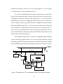
The generalization of such a multiprocessor chip is one that has a collec-
video-conferencing, etc.
tion of programmable processors as well as custom hardware on a single chip.
The idea of using multiple processing units to execute one program has
Mapping applications onto such an architecture is then a hardware/software code-
been present from the time of the very first electronic computer in the nineteen for-
sign problem. The problems of inter-processor communication and synchroniza-
ties. Parallel computation has since been the topic of active research in computer
tion are identical to the homogeneous multiprocessor case. In this thesis when we
science. Whereas parallelism within a single processor has been successfully
refer to a “multiprocessor” we will imply a heterogeneous architecture that may be
exploited (instruction-level parallelism), the problem of partitioning a single user
comprised of different types of programmable processors and may include custom
program onto multiple such processors is yet to be satisfactorily solved. Instruc-
hardware elements too. All the techniques we present here apply to such a general
tion-level parallelism includes techniques such as pipelining (employed in tradi-
system architecture.
tional RISC processors), vectorization, VLIW (very large instruction word),
Why study application-specific parallel processing in the first place instead
superscalar — these techniques are discussed in detail by Patterson and Hennessy
of applying the ideas in general purpose parallel systems to the specific applica-
in [Patt90]. Architectures that employ multiple CPUs to achieve task-level paral-
tion? The reason is that general purpose parallel computation deals with a user-
lelism fall into the shared memory, message passing, or dataflow paradigms. The
programmable computing device. Computation in embedded applications, how-
Stanford DASH multiprocessor [Len92] is a shared memory machine whereas the
ever, is usually one-time programmed by the designer of that embedded system (a
Thinking Machines CM-5 falls into the message passing category. The MIT Mon-
digital cellular radio handset for example) and is not meant to be programmable by
soon machine [Pap90] is an example of a dataflow architecture.
the end user. The computation in embedded systems is specialized (the computa3
Although the hardware for the design of such multiple processor machines
4
— the memory, interconnect network, IO, etc. — has received much attention,
BDF model can therefore compute all Turing computable functions, whereas this
software for such machines has not been able to keep up with the hardware devel-
is not possible in the case of the SDF model. We discuss the Boolean dataflow
opment. Efficient partitioning of a general program (written in C say) across a
model further in Chapter 6.
given set of processors arranged in a particular configuration is still an open prob-
In exchange for the limited expressivity of an SDF representation, we can
lem. Detecting parallelism, the overspecified sequencing in popular imperative
efficiently check conditions such as whether a given SDF graph deadlocks, and
languages like C, managing overhead due to communication and synchronization
whether it can be implemented using a finite amount of memory. No such general
between processors, and the requirement of dynamic load balancing for some pro-
procedures can be devised for checking the corresponding conditions (deadlock
grams (an added source of overhead) makes the partitioning problem for a general
behaviour and bounded memory usage) for a computation model that can simulate
program hard.
any given Turing machine. This is because the problems of determining if any
If we turn away from general purpose computation to application-specific
given Turing machine halts (the halting problem), and determining whether it will
domains, however, parallelism is easier to identify and exploit. For example, one
use less than a given amount of memory (or tape) are undecidable [Lew81]; that is,
of the more extensively studied family of such application-specific parallel proces-
no general algorithm exists to solve these problems in finite time.
sors is the systolic array architecture [Kung88][Quin84][Rao85]; this architecture
In this thesis we will first focus on techniques that apply to SDF applica-
consists of regularly arranged arrays of processors that communicate locally, onto
tions, and we will propose extensions to these techniques for applications that can
which a certain class of applications, specified in a mathematical form, can be sys-
be specified essentially as SDF, but augmented with a limited number of control
tematically mapped. We discuss systolic arrays further in section 1.3.2.
constructs (and hence fall into the BDF model). SDF has proven to be a useful
The necessary elements in the study of application-specific computer archi-
model for representing a significant class of DSP algorithms; several DSP tools
tectures are: 1) a clearly defined set of problems that can be solved using the par-
have been designed based on the SDF and closely related models. Examples of
ticular application-specific approach, 2) a formal mechanism for specification of
commercial tools based on SDF are the Signal Processing Worksystem (SPW),
these applications, and 3) a systematic approach for designing hardware from such
developed by Comdisco Systems (now the Alta group of Cadence Design Sys-
a specification.
tems) [Pow92][Barr91]; and COSSAP, developed by Cadis in collaboration with
In this thesis, the applications we focus on are those that can be described
Meyr’s group at Aachen University [Ritz92]. Tools developed at various universi-
by Synchronous Dataflow Graphs (SDF) [Lee87] and its extensions; we will dis-
ties that use SDF and related models include Ptolemy [Pin95a], the Warp compiler
cuss this model in detail shortly. SDF in its pure form can only represent applica-
[Prin92], DESCARTES [Ritz92], GRAPE [Lauw90], and the Graph Compiler
tions that have no decision making at the task level. Extensions of SDF (such as
[Veig90].
the Boolean dataflow (BDF) model [Lee91][Buck93]) allow control constructs, so
The SDF model is popular because it has certain analytical properties that
that data-dependent control flow can be expressed in such models. These models
are useful in practice; we will discuss these properties and how they arise in the
are significantly more powerful in terms of expressivity, but they give up some of
following section. The property most relevant for this thesis is that it is possible to
the useful analytical properties that the SDF model has. For instance, Buck shows
effectively exploit parallelism in an algorithm specified in SDF by scheduling
that it is possible to simulate any Turing machine in the BDF model [Buck93]. The
computations in the SDF graph onto multiple processors at compile or design time
5
6
rather than at run time. Given such a schedule that is determined at compile time,
ties that facilitate formal reasoning about programs specified in these models, and
we can extract information from it with a view towards optimizing the final imple-
are useful in practise, leading to simpler implementation of the specified computa-
mentation. The main contribution of this thesis is to present techniques for mini-
tion in hardware or software.
mizing synchronization and inter-processor communication overhead in statically
One such restricted model (and in fact one of the earliest graph based com-
(i.e. compile time) scheduled multiprocessors where the program is derived from a
putation models) is the computation graph of Karp and Miller [Karp66]. In their
dataflow graph specification. The strategy is to model run time execution of such a
seminal paper Karp and Miller establish that their computation graph model is
multiprocessor to determine how processors communicate and synchronize, and
determinate, i.e. the sequence of tokens produced on the edges of a given computa-
then to use this information to optimize the final implementation.
tion graph are unique, and do not depend on the order that the actors in the graph
fire, as long as all data dependencies are respected by the firing order. The authors
1.1
1.1.1
The Synchronous Dataflow model
also provide an algorithm that, based on topological and algebraic properties of the
graph, determines whether the computation specified by a given computation
Background
graph will eventually terminate. Because of the latter property, computation graphs
Dataflow is a well-known programming model in which a program is rep-
clearly cannot simulate all Turing machines, and hence are not as expressive as a
resented as a directed graph, where the vertices (or actors) represent computation
general dataflow language like Lucid or pure LISP. Computation graphs provide
and edges (or arcs) represent FIFO (first-in-first-out) queues that direct data values
some of the theoretical foundations for the SDF model.
from the output of one computation to the input of another. Edges thus represent
Another model of computation relevant to dataflow is the Petri net model
data precedences between computations. Actors consume data (or tokens) from
[Peter81][Mur89]. A Petri net consists of a set of transitions, which are analogous
their inputs, perform computation on them (fire), and produce certain number of
to actors in dataflow, and a set of places that are analogous to arcs. Each transition
tokens on their outputs.
has a certain number of input places and output places connected to it. Places may
Programs written in high-level functional languages such as pure LISP, and
contain one or more tokens. A Petri net has the following semantics: a transition
in dataflow languages such as Id and Lucid can be directly converted into dataflow
fires when all its input places have one or more tokens and, upon firing, it produces
graph representations; such a conversion is possible because these languages are
a certain number of tokens on each of its output places.
designed to be free of side-effects, i.e. programs in these languages are not allowed
A large number of different kinds of Petri net models have been proposed
to contain global variables or data structures, and functions in these languages can-
in the literature for modeling different types of systems. Some of these Petri net
not modify their arguments [Ack82]. Also, since it is possible to simulate any Tur-
models have the same expressive power as Turing machines: for example if transi-
ing machine in one of these languages, questions such as deadlock (or,
tions are allowed to posses “inhibit” inputs (if a place corresponding to such an
equivalently, terminating behaviour) and determining maximum buffer sizes
input to a transition contains a token, then that transition is not allowed to fire) then
required to implement edges in the dataflow graph become undecidable. Several
a Petri net can simulate any Turing machine (pp. 201 in [Peter81]). Others
models based on dataflow with restricted semantics have been proposed; these
(depending on topological restrictions imposed on how places and transitions can
models give up the descriptive power of general dataflow in exchange for proper-
be interconnected) are equivalent to finite state machines, and yet others are simi-
7
8
lar to SDF graphs. Some extended Petri net models allow a notion of time, to
is not possible for a general dataflow model); consequently, buffers can be allo-
model execution times of computations. There is also a body of work on stochastic
cated statically, and run time overhead associated with dynamic memory allocation
extensions of timed Petri nets that are useful for modeling uncertainties in compu-
is avoided. The existence of a periodic schedule that can be inferred at compile
tation times. We will touch upon some of these Petri net models again in Chapter
time implies that a correctly constructed SDF graph entails no run time scheduling
4. Finally, there are Petri nets that distinguish between different classes of tokens
overhead.
in the specification (colored Petrinets), so that tokens can have information associ-
An SDF graph in which every actor consumes and produces only one token
ated with them. We refer to [Peter81] [Mur89] for details on the extensive variety
from each of its inputs and outputs is called a homogeneous SDF graph
of Petri nets that have been proposed over the years.
(HSDFG). An HSDF graph actor fires when it has one or more tokens on all its
The particular restricted dataflow model we are mainly concerned with in
input edges; it consumes one token from each input edge when it fires, and pro-
this thesis is the SDF — Synchronous Data Flow — model proposed by Lee and
duces one token on all its output edges when it completes execution. A general
Messerschmitt [Lee87]. The SDF model poses restrictions on the firing of actors:
(multirate) SDF graph can always be converted into an HSDF graph [Lee86]; this
the number of tokens produced (consumed) by an actor on each output (input)
transformation may result in an exponential increase in the number of actors in the
edge is a fixed number that is known at compile time. The arcs in an SDF graph
final HSDF graph (see [Pin95b] for an example of an SDF graph in which this
may contain initial tokens, which we also refer to as delays. Arcs with delays can
blowup occurs). Such a transformation, however, appears to be necessary when
be interpreted as data dependencies across iterations of the graph; this concept will
constructing periodic multiprocessor schedules from multirate SDF graphs. There
be formalized in the following chapter. In an actual implementation, arcs represent
is some recent work on reducing the complexity of the HSDFG that results from
buffers in physical memory.
transforming a given SDF graph by applying graph clustering techniques to that
DSP applications typically represent computations on an indefinitely long
SDF graph [Pin95b]. Since we are concerned with multiprocessor schedules in this
data sequence; therefore the SDF graphs we are interested in for the purpose of
thesis, we assume we start with an application represented as a homogeneous SDF
signal processing must execute in a nonterminating fashion. Consequently, we
graph henceforth, unless we state otherwise. This of course results in no loss of
must be able to obtain periodic schedules for SDF representations, which can then
generality because a multirate graph is converted into a homogeneous graph for
be run as infinite loops using a finite amount of physical memory. Unbounded
the purposes of multiprocessor scheduling anyway. In Chapter 6 we discuss how
buffers imply a sample rate inconsistency, and deadlock implies that all actors in
the ideas that apply to HSDF graphs can be extended to graphs containing actors
the graph cannot be iterated indefinitely. Thus for our purposes, correctly con-
that display data-dependent behaviour (i.e. dynamic actors).
structed SDF graphs are those that can be scheduled periodically using a finite
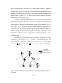
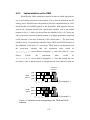
We note that an HSDFG is very similar to a marked graph in the context
amount of memory. The main advantage of imposing restrictions on the SDF
of Petri nets [Peter81]; transitions in the marked graph correspond to actors in the
model (over a general dataflow model) lies precisely in the ability to determine
HSDFG, places correspond to edges, and initial tokens (or initial marking) of the
whether or not an arbitrary SDF graph has a periodic schedule that neither dead-
marked graph correspond to initial tokens (or delays) in HSDFGs. We will repre-
locks nor requires unbounded buffer sizes [Lee87]. The buffer sizes required to
sent delays using bullets (•) on the edges of the HSDFG; we indicate more than
implement arcs in SDF graphs can be determined at compile time (recall that this
one delay on an edge by a number alongside the bullet, as in Fig. 1.1(a).
9
10
SDF should not be confused with synchronous languages [Hal93][Ben91]
the functional or behavioural level, and for synthesis from such a high level speci-
(e.g. LUSTRE, SIGNAL, and ESTEREL), which have very different semantics
fication to a software description (e.g. a C program) or a hardware description (e.g.
from SDF. Synchronous languages have been proposed for formally specifying
VHDL) or a combination thereof. The descriptions thus generated can then be
and modeling reactive systems, i.e. systems that constantly react to stimuli from a
compiled down to the final implementation, e.g. an embedded processor, or an
given physical environment. Signal processing systems fall into the reactive cate-
ASIC.
gory, and so do control and monitoring systems, communication protocols, man-
One of the reasons for the popularity of such dataflow based models is that
machine interfaces, etc. In these languages variables are possibly infinite
they provide a formalism for block-diagram based visual programming, which is a
sequences of data of a certain type. Associated with each such sequence is a con-
very intuitive specification mechanism for DSP; the expressivity of the SDF model
ceptual (and sometimes explicit) notion of a clock signal. In LUSTRE, each vari-
sufficiently encompasses a significant class of DSP applications, including multi-
able is explicitly associated with a clock, which determines the instants at which
rate applications that involve upsampling and downsampling operations. An
the value of that variable is defined. SIGNAL and ESTEREL do not have an
equally important reason for employing dataflow is that such a specification
explicit notion of a clock. The clock signal in LUSTRE is a sequence of Boolean
exposes parallelism in the program. It is well known that imperative programming
values, and a variable in a LUSTRE program assumes its n th value when its corre-
styles such as C and FORTRAN tend to over-specify the control structure of a
sponding clock takes its n th TRUE value. Thus we may relate one variable with
given computation, and compilation of such specifications onto parallel architec-
another by means of their clocks. In ESTEREL, on the other hand, clock ticks are
tures is known to be a hard problem. Dataflow on the other hand imposes minimal
implicitly defined in terms of instants when the reactive system corresponding to
data-dependency constraints in the specification, potentially enabling a compiler to
an ESTEREL program receives (and reacts to) external events. All computations
detect parallelism. The same argument holds for hardware synthesis, where it is
in synchronous language are defined with respect to these clocks.
important to be able to exploit concurrency.
In contrast, the term “synchronous” in the SDF context refers to the fact
The SDF model has also proven useful for compiling DSP applications on
that SDF actors produce and consume fixed number of tokens, and these numbers
single processors. Programmable digital signal processing chips tend to have spe-
are known at compile time. This allows us to obtain periodic schedules for SDF
cial instructions such as a single cycle multiply-accumulate (for filtering func-
graphs such that the average rates of firing of actors are fixed relative to one
tions), modulo addressing (for managing delay lines), bit-reversed addressing (for
another. We will not be concerned with synchronous languages in this thesis,
FFT computation); DSP chips also contain built in parallel functional units that are
although these languages have a close and interesting relationship with dataflow
controlled from fields in the instruction (such as parallel moves from memory to
models used for specification of signal processing algorithms [Lee95].
registers combined with an ALU operation). It is difficult for automatic compilers
to optimally exploit these features; executable code generated by commercially
1.1.2
Utility of dataflow for DSP
available compilers today utilizes one and a half to two times the program memory
As mentioned before, dataflow models such as SDF (and other closely
that a corresponding hand optimized program requires, and results in two to three
related models) have proven to be useful for specifying applications in signal pro-
times higher execution time compared to hand-optimized code [Zivo95]. There has
cessing and communications, with the goal of both simulation of the algorithm at
been some recent work on compilation techniques for embedded software target-
11
12
ted towards DSP processors and microcontrollers [Liao95]; it is still too early to
actor fires such that all data precedence constraints are met. Each of these three
determine the impact of these techniques on automatic compilation for large-scale
tasks may be performed either at run time (a dynamic strategy) or at compile time
DSP/control applications, however.
(static strategy). We restrict ourselves to non-preemptive schedules, i.e. schedules
Block diagram languages based on models such as SDF have proven to be
where an actor executing on a processor can not be interrupted in the middle of its
a bridge between automatic compilation and hand coding approaches; a library of
execution to allow another task to be executed. This is because preemption entails
reusable blocks in a particular programming language is hand coded, this library
a significant implementation overhead and is therefore of limited use in embedded,
then constitutes the set of atomic SDF actors. Since the library blocks are reusable,
time-critical applications.
one can afford to carefully optimize and fine tune them. The atomic blocks are fine
Lee and Ha [Lee89] propose a scheduling taxonomy based on which of the
to medium grain in size; an atomic actor in the SDF graph may implement any-
scheduling tasks are performed at compile time and which at run time; we use the
thing from a filtering function to a two input addition operation. The final program
same terminology in this thesis. To reduce run time computation costs it is advan-
is then automatically generated by concatenating code corresponding to the blocks
tageous to perform as many of the three scheduling tasks as possible at compile
in the program according to the sequence prescribed by a schedule. This approach
time, especially in the context of algorithms that have hard real-time constraints.
is mature enough that there are commercial tools available today, for example the
Which of these can be effectively performed at compile time depends on the infor-
SPW and COSSAP tools mentioned earlier, that employ this technique. Powerful
mation available about the execution time of each actor in the HSDFG.
optimization techniques have been developed for generating sequential programs
from SDF graphs that optimize for metrics such as memory usage [Bhat94].
For example, dataflow computers first pioneered by Dennis [Denn80] perform the assignment step at compile time, but employ special hardware (the token-
Scheduling is a fundamental operation that must be performed in order to
match unit) to determine, at runtime, when actors assigned to a particular proces-
implement SDF graphs on both uniprocessor as well as multiprocessors. Unipro-
sor are ready to fire. The runtime overhead of token-matching and dynamic sched-
cessor scheduling simply refers to determining the sequence of execution of actors
uling (within each processor) is fairly severe, so much so that dataflow
such that all precedence constraints are met and all the buffers between actors (cor-
architectures have not been commercially viable; even with expensive hardware
responding to arcs) return to their initial states. We discuss the issues involved in
support for dynamic scheduling, performance of such computers has been unim-
multiprocessor scheduling next.
pressive.
1.2
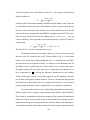
iteration period T : the average time it takes for all the actors in the graph to be
The performance metric of interest for evaluating schedules is the average
Parallel scheduling
executed once. Equivalently, we could use the throughput T
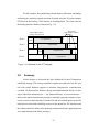
We recall that in the execution of a dataflow graph, actors fire when sufficient number of tokens are present at their inputs. The task of scheduling such a
actors on each processor (the actor ordering step), and determining when each
(i.e. the number of
iterations of the graph executed per unit time) as a performance metric. Thus an
optimal schedule is one that minimizes T .
graph onto multiple processing units therefore involves assigning actors in the
HSDFG to processors (the processor assignment step), ordering execution of these
–1
In this thesis we focus on scheduling strategies that perform both processor
assignment and actor ordering at compile time, because these strategies appear to
be most useful for a significant class of real time DSP algorithms. Although
13
14
assignment and ordering performed at run time would in general lead to a more
flexible implementation (because a dynamic strategy allows for run time variations
in computation load and for operations that display data dependencies) the over-
B
head involved in such a strategy is usually prohibitive and real-time performance
C
B
C
D
A
D
Proc 1 C A
B
Proc 2 D
t
2
guarantees are difficult to achieve. Lee and Ha [Lee89] define two scheduling
strategies that perform the assignment and ordering steps at compile time: fullystatic and self-timed. We use the same terminology in this thesis.
1.2.1
A
(a) HSDFG
Proc 1 C A
C A
C A
Proc 2 D
B D
B D
acyclic precedence graph
T=3 t.u.
(b) blocked schedule
Fully-static schedules
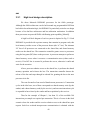
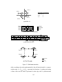
In the fully-static (FS) strategy, the exact firing time of each actor is also
determined at compile time. Such a scheduling style is used in the design of systolic array architectures [Kung88], for scheduling VLIW processors [Lam88], and
Proc 1
Proc 2
Proc 1
C B
Proc 2 D A
t
T = 2 t.u.
in high-level VLSI synthesis of applications that consist only of operations with
guaranteed worst-case execution times [DeMich94]. Under a fully static schedule,
C B C B C B A
B
D A D A D A D
(c) overlapped schedule
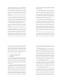
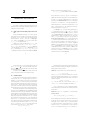
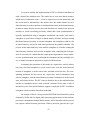
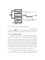
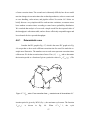
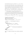
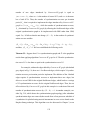
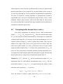
Figure 1.1. Fully static schedule
all processors run in lock step; the operation each processor performs on each
clock cycle is predetermined at compile time and is enforced at run time either
implicitly (by the program each processor executes, perhaps augmented with
“nop”s or idle cycles for correct timing) or explicitly (by means of a program
on how successive iterations of the HSDFG are treated. Execution times of all
actors are assumed to be one time unit (t.u.) in this example. The FS schedule in
Fig. 1.1(b) represents a blocked schedule: successive iterations of the HSDFG in a
blocked schedule are treated separately so that each iteration is completed before
sequencer for example).
A fully-static schedule of a simple HSDFG G is illustrated in Fig. 1.1. The
FS schedule is schematically represented as a Gantt chart that indicates the processors along the vertical axis, and time along the horizontal axis. The actors are represented as rectangles with horizontal length equal to the execution time of the
actor. The left side of each actor in the Gantt chart corresponds to its starting time.
The Gantt chart can be viewed as a processor-time plane; scheduling can then be
viewed as a mechanism to tile this plane while minimizing total schedule length
and idle time (“empty spaces” in the tiling process). Clearly, the FS strategy is viable only if actor execution time estimates are accurate and data-independent or if
tight worst-case estimates are available for these execution times.
As shown in Fig. 1.1, two different types of FS schedules arise, depending
15
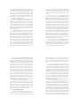
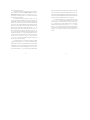
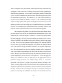
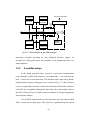
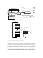
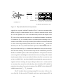
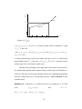
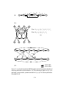
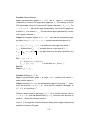
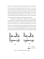
the next one begins. A more elaborate blocked schedule on five processors is
shown in Fig. 1.2. The HSDFG is scheduled as if it executes for only one iteration,
i.e. inter-iteration dependencies are ignored; this schedule is then repeated to get
an infinite periodic schedule for the HSDFG. The length of the blocked schedule
determines the average iteration period T . The scheduling problem is then to
obtain a schedule that minimizes T (which is also called the makespan of the
schedule). A lower bound on T for a blocked schedule is simply the length of the
critical path of the graph, which is the longest delay-free path in the graph.
Ignoring the inter-iteration dependencies when scheduling an HSDFG is
equivalent to the classical multiprocessor scheduling problem for an Acyclic Precedence Graph (APG): the acyclic precedence graph is obtained from the given
16
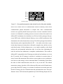
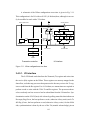
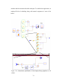
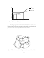
The heuristics mentioned above ignore communication costs between proProc 1
A
•
•
E
H
•
B
Proc 5
F
Proc 1
Execution Times
D
A , B, F
C, H
D
E
G
Proc 4
Proc 3
C
G
Proc 2
:6
:4
Proc 2
Proc 3
Proc 4
:2
Proc 5
:3
:5
r1
B
G
E
A
s6
C
r3
D
s6
r4
s3
H
cessors, which is often inappropriate in actual multiprocessor implementations. An
s5
F
r2
s1
s4
s2
ment step represents interprocessor communication (IPC) (illustrated in Fig.
r5
1.3(a)). These communication points are usually implemented using send and
= Idle
receive primitives that make use of the processor interconnect hardware. These
(b) Static schedule
(a) HSDFG “G”
edge of the HSDFG that crosses processor boundaries after the processor assign-
primitives then have an execution cost associated with them that depends on the
multiprocessor architecture and hardware being employed. Fully-static scheduling
TFS=11
Proc 1
E
Proc 2
Proc 3
Proc 4
B
E
A
B
F
C
G
C
C
10
heuristics
20
take
communication
costs
into
account
include
Computations in the HSDFG, however, are iterated essentially infinitely.
H
15
that
[Sark89][Sih91][Prin91].
D
H
5
A
F
G
D
H
0
B
F
G
D
Proc 5
E
A
t
The blocked scheduling strategies discussed thus far ignore this fact, and thus pay
a penalty in the quality of the schedule they obtain. Two techniques that enable
(c) Fully-static execution
Figure 1.2. Fully-static schedule on five processors
blocked schedules to exploit inter-iteration parallelism are unfolding and retiming. The unfolding strategy schedules J iterations of the HSDFG together, where
HSDFG by eliminating all edges with delays on them (edges with delays represent
J is called the blocking factor. Thus the schedule in Fig. 1.1(b) has J = 1 .
dependencies across iterations) and replacing multiple edges that are directed
Unfolding often leads to improved blocked schedules (pp. 78-100 [Lee86],
between the same two vertices in the same direction with a single edge. This
[Parhi91]), but it also implies a factor of J increase in program memory size and
replacement is done because such multiple edges represent identical precedence
also in the size of the scheduling problem, which makes unfolding somewhat
constraints; these edges are taken into account individually during buffer assign-
impractical.
ment, however. Optimal multiprocessor scheduling of an acyclic graph is known to
Retiming involves manipulating delays in the HSDFG to reduce the critical
be NP-Hard [Garey79], and a number of heuristics have been proposed for this
path in the graph. This technique has been explored in the context of maximizing
problem. One of the earliest, and still popular, solutions to this problem is list
clock rates in synchronous digital circuits [Lei83], and has been proposed for
scheduling, first proposed by Hu [Hu61]. List scheduling is a greedy approach:
improving blocked schedules for HSDFGs (“cutset transformations” in [Lee86],
whenever a task is ready to run, it is scheduled as soon as a processor is available
and [Hoang93]).
to run it. Tasks are assigned priorities, and among the tasks that are ready to run at
Fig. 1.1(c) illustrates an example of an overlapped schedule. Such a
any instant, the task with the highest priority is executed first. Various researchers
schedule is explicitly designed such that successive iterations in the HSDFG over-
have proposed different priority mechanisms for list scheduling [Adam74], some
lap. Obviously, overlapped schedules often achieve a lower iteration period than
of which use critical path based (CPM) methods [Ram72][Koh75][Blaz87]
blocked schedules. In Fig. 1.1, for example, the iteration period for the blocked
([Blaz87] summarizes a large number of CPM based heuristics for scheduling).
schedule is 3 units whereas it is 2 units for the overlapped schedule. One might
17
18
wonder whether overlapped schedules are fundamentally superior to blocked
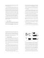
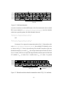
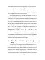
(b)), we simply discard the timing information that is not required, and only retain
schedules with the unfolding and retiming operations allowed. This question is set-
the processor assignment and the ordering of actors on each processor as specified
tled in the affirmative by Parhi and Messerschmitt [Parhi91]; the authors provide
by the FS schedule (Fig. 1.3(c)). Each processor is assigned a sequential list of
an example of an HSDFG for which no blocked schedule can be found, even
actors, some of which are send and receive actors, that it executes in an infinite
allowing unfolding and retiming, that has a lower or equal iteration period than the
loop. When a processor executes a communication actor, it synchronizes with the
overlapped schedule they propose.
processor(s) it communicates with. Exactly when a processor executes each actor
Optimal resource constrained overlapped scheduling is of course NP-Hard,
depends on when, at run time, all input data for that actor are available, unlike the
although a periodic overlapped schedule in the absence of processor constraints
fully-static case where no such run time check is needed. Conceptually, the proces-
can be computed efficiently and optimally [Parhi91][Gasp92].
sor sending data writes data into a FIFO buffer, and blocks when that buffer is full;
Overlapped scheduling heuristics have not been as extensively studied as
the receiver on the other hand blocks when the buffer it reads from is empty. Thus
blocked schedules. The main work in this area is by Lam [Lam88], and deGroot
flow control is performed at run time. The buffers may be implemented using
[deGroot92], who propose a modified list scheduling heuristic that explicitly con-
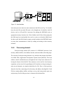
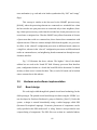
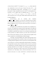
shared memory, or using hardware FIFOs between processors. In a self-timed
structs an overlapped schedule. Another work related to overlapped scheduling is
strategy, processors run sequential programs and communicate when they execute
the “cyclo-static scheduling” approach proposed by Schwartz. This approach
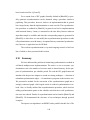
the communication primitives embedded in their programs, as shown schemati-
attempts to optimally tile the processor-time plane to obtain the best possible
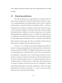
cally in Fig. 1.3 (c).
schedule. The search involved in this process has a worst case complexity exponential in the size of the input graph, although it appears that the complexity is
manageable in practice, at least for small examples [Schw85].
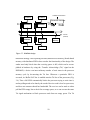
1.2.2
Self-timed schedules
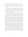
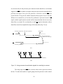
The fully-static approach introduced in the previous section cannot be used
when actors have variable execution times; the FS approach requires precise
A
s
r
D
Proc 1 D
Proc 2 C
r
s
A
B
t
C
B
(b) Fully-static schedule
(a) HSDFG
Proc 1
Proc 2
start
start
rec
C
D
rec
A
send
B
send
(c) Self-timed implementation
(schematic)
knowledge of actor execution times to guarantee sender-receiver synchronization.
It is possible to use worst case execution times and still employ an FS strategy, but
this requires tight worst case execution time estimates that may not be available to
Figure 1.3. Steps in a self-timed scheduling strategy
us. An obvious strategy for solving this problem is to introduce explicit synchroni-
An ST strategy is robust with respect to changes in execution times of
zation whenever processors communicate. This leads to the self-timed scheduling
actors, because sender-receiver synchronization is performed at run time. Such a
(ST) strategy in the scheduling taxonomy of Lee and Ha [Lee89]. In this strategy
strategy, however, implies higher IPC costs compared to the fully-static strategy
we first obtain an FS schedule using the techniques discussed in section 1.2, mak-
because of the need for synchronization (e.g. using semaphore management). In
ing use of the execution time estimates. After computing the FS schedule (Fig. 1.3
addition the ST strategy faces arbitration costs: the FS schedule guarantees mutu-
19
20
ally exclusive access of shared communication resources, whereas shared
magnitude occasionally occur due to phenomena such as cache misses, interrupts,
resources need to be arbitrated at run time in the ST schedule. Consequently,
user inputs or error handling. Consequently, tight worst-case execution time
whereas IPC in the FS schedule simply involves reading and writing from shared
bounds cannot generally be determined for such operations; however, reasonably
memory (no synchronization or arbitration needed), implying a cost of a few pro-
good execution time estimates can in fact be obtained for these operations, so that
cessor cycles for IPC, the ST strategy requires of the order of tens of processor
static assignment and ordering techniques are viable. For such applications self-
cycles, unless special hardware is employed for run time flow control. We discuss
timed scheduling is ideal, because the performance penalty due to lack of dynamic
in detail how this overhead arises in a shared bus multiprocessor configuration in
load balancing is overcome by the much smaller run time scheduling overhead
Chapter 3.
involved when static assignment and ordering is employed.
Run time flow control allows variations in execution times of tasks; in
The estimates for execution times of actors can be obtained by several dif-
addition, it also simplifies the compiler software, since the compiler no longer
ferent mechanisms. The most straightforward method is for the programmer to
needs to perform detailed timing analysis and does not need to adjust the execution
provide these estimates when he writes the library of primitive blocks. This strat-
of processors relative to one another in order to ensure correct sender-receiver syn-
egy is used in the Ptolemy system, and is very effective for the assembly code
chronization. Multiprocessor designs, such as the Warp array [Ann87][Lam88] and
libraries, in which the primitives are written in the assembly language of the target
the 2-D MIMD (Multiple Instruction Multiple Data) array of [Ziss87], that could
processor (Ptolemy currently supports the Motorola 56000 and 96000 processors).
potentially use fully-static scheduling, still choose to implement such run time
The programmer can provide a good estimate for blocks written in such a library
flow control (at the expense of additional hardware) for the resulting software sim-
by counting the number of processor cycles each instruction consumes, or by pro-
plicity. Lam presents an interesting discussion on the trade-off involved between
filing the block on an instruction-set simulator.
hardware complexity and ease of compilation that ensues when we consider
It is more difficult to estimate execution times for blocks that contain con-
dynamic flow control implemented in hardware versus static flow control enforced
trol constructs such as data-dependent iterations and conditionals within their
by a compiler (pp. 50-68 of [Lam89]).
body, and when the target processor employs pipelining and caching. Also, it is
difficult, if not impossible, for the programmer to provide reasonably accurate esti-
1.2.3
Execution time estimates and static schedules
mates of execution times for blocks written in a high-level language (as in the C
We assume we have reasonably good estimates of actor execution times
code generation library in Ptolemy). The solution adopted in the GRAPE system
available to us at compile time to enable us to exploit static scheduling techniques;
[Lauw90] is to automatically estimate these execution times by compiling the
however, these estimates need not be exact, and execution times of actors may
block (if necessary) and running it by itself in a loop on an instruction-set simula-
even be data-dependent. Thus we allow actors that have different execution times
tor for the target processor. To take into account data-dependent execution behav-
from one iteration of the HSDFG to the next, as long as these variations are small
iour, different input data sets can be provided for the block during simulation.
or rare. This is typically the case when estimates are available for the task execu-
Either the worst case or the average case execution time is used as the final esti-
tion times, and actual execution times are close to the corresponding estimates
mate.
with high probability, but deviations from the estimates of (effectively) arbitrary
The estimation procedure employed by GRAPE is obviously time consum-
21
ing; in fact estimation turns out to be the most time consuming step in the GRAPE
22
1.3
design flow. Analytical techniques can be used instead to reduce this estimation
time; for example, Li and Malik [Li95] have proposed algorithms for estimating
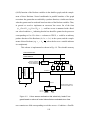
the execution time of embedded software. Their estimation technique, which
forms a part of a tool called cinderella, consists of two components: 1) determining the sequence of instructions in the program that results in maximum execution
time (program path analysis) and 2) modeling the target processor to determine
Application-specific parallel architectures
There has been significant amount of research on general purpose high-
performance parallel computers. These employ expensive and elaborate interconnect topologies, memory and Input/Output (I/O) structures. Such strategies are
unsuitable for embedded DSP applications as we discussed earlier. In this section
we discuss some application-specific parallel architectures that have been
employed for signal processing, and contrast them to our approach.
how much time the worst case sequence determined in step 1 takes to execute
(micro-architecture modeling). The target processor model also takes the effect of
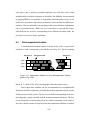
1.3.1
Dataflow DSP architectures
instruction pipelines and cache activity into account. The input to the tool is a
There have been a few multiprocessors geared towards signal processing
generic C program with annotations that specify the loop bounds (i.e. the maxi-
that are based on the dataflow architecture principles of Dennis [Denn80]. Notable
mum number of iterations that a loop runs for). Although the problem is formu-
among these are Hughes Data Flow Multiprocessor [Gau85], the Texas Instru-
lated as an integer linear program (ILP), the claim is that practical inputs to the
ments Data Flow Signal Processor [Grim84], and the AT&T Enhanced Modular
tool can be efficiently analyzed using a standard ILP solver. The advantage of this
Signal Processor [Bloch86]. The first two perform the processor assignment step at
approach, therefore, is the efficient manner in which estimates are obtained as
compile time (i.e. tasks are assigned to processors at compile time) and tasks
compared to simulation.
assigned to a processor are scheduled on it dynamically; the AT&T EMPS per-
It should be noted that the program path analysis component of the Li and
forms even the assignment of tasks to processors at runtime.
Malik technique is in general an undecidable problem; therefore for these tech-
Each one of these machines employs elaborate hardware to implement
niques to function, the programmer must ensure that his or her program does not
dynamic scheduling within processors, and employs expensive communication
contain pointer references, dynamic data structures, recursion, etc. and must pro-
networks to route tokens generated by actors assigned to one processor to tasks on
vide bounds on all loops. Li and Malik’s technique also depends on the accuracy of
other processors that require these tokens. In most DSP applications, however,
the processor model, although one can expect good models to eventually evolve
such dynamic scheduling is unnecessary since compile time predictability makes
for DSP chips and microcontrollers that are popular in the market.
static scheduling techniques viable. Eliminating dynamic scheduling results in
The problem of estimating execution times of blocks is central for us to be
much simpler hardware without an undue performance penalty.
able to effectively employ compile time design techniques. This problem is an
Another example of an application-specific dataflow architecture is the
important area of research in itself, and the strategies employed in Ptolemy and
NEC µPD7281 [Chase84], which is a single chip processor geared towards image
GRAPE, and those proposed by Li and Malik are useful techniques, and we expect
processing. Each chip contains one functional unit; multiple such chips can be
better estimation techniques to be developed in the future.
connected together to execute programs in a pipelined fashion. The actors are statically assigned to each processor, and actors assigned to a given processor are
23
24
scheduled on it dynamically. The primitives that this chip supports, convolution,
of a programmable systolic array, as opposed to a dedicated array designed for one
bit manipulations, accumulation, etc., are specifically designed for image process-
specific application. Processors are arranged in a linear array and communicate
ing applications.
with their neighbors through FIFO queues. Programs are written for this computer
in a language called W2 [Lam88]. The Warp project also led to the iWarp design
1.3.2
Systolic and wavefront arrays
[Bork88], which has a more elaborate inter-processor communication mechanism
Systolic arrays consist of processors that are locally connected and may be
than the Warp machine. An iWarp node is a single VLSI component, composed of
arranged in different topologies: mesh, ring, torus, etc. The term “systolic” arises
a computation engine and a communication engine; the latter consists of a crossbar
because all processors in such a machine run in lock-step, alternating between a
and data routing mechanisms. The iWarp nodes can be connected in various single
computation step and a communication step. The model followed is usually SIMD
and two dimensional topologies, and point to point message-passing type commu-
(Single Instruction Multiple Data). Systolic arrays can execute a certain class of
nication is supported.
problems that can be specified as “Regular Iterative Algorithms (RIA)” [Rao85];
systematic techniques exist for mapping an algorithm specified in a RIA form onto
1.3.3
as processor and communication link utilization, scalability with the problem size,
Multiprocessor DSP architectures
In this section we discuss multiprocessors that make use of multiple off the
dedicated processor arrays in an optimal fashion. Optimality includes metrics such
shelf programmable DSP chips.
achieving best possible speedup for a given number of processors, etc. Several
The SMART architecture [Koh90] is a reconfigurable bus design com-
numerical computation problems were found to fall into the RIA category: linear
prised of AT&T DSP32C processors, and custom VLSI components for routing
algebra,
(see
data between processors. Clusters of processors may be connected onto a common
[Kung88][Leigh92] for interesting systolic array implementations of a variety of
bus, or may form a linear array with neighbor to neighbor communication. This
different numerical problems). Only fairly regular computations can be specified
allows the multiprocessor to be reconfigured depending on the communication
in the RIA form; this makes the applicability of systolic arrays somewhat restric-
requirement of the particular application being mapped onto it. Scheduling and
tive.
code generation for this machine is done by the McDAS compiler [Hoang93].
matrix
operations,
singular
value
decomposition,
etc.
Wavefront arrays are similar to systolic arrays except that processors are
The DSP3 multiprocessor [Shive92] was built at AT&T, and is comprised
not under the control of a global clock. Communication between processors is
of DSP32C processors connected in a mesh configuration. The mesh interconnect
asynchronous or self-timed; handshake between processors ensures run time syn-
is implemented using custom VLSI components for data routing. Each processor
chronization. Thus processors in a wavefront array can be complex and the arrays
communicates with four of its adjacent neighbors through this router, which con-
themselves can consist of a large number of processors without incurring the asso-
sists of input and output queues, and a crossbar that is configurable under program
ciated problems of clock skew and global synchronization. Again, similar to FS
control. Data packets contain headers that indicate the ID of the destination proces-
versus ST scheduling, the flexibility of wavefront arrays over systolic arrays
sor.
comes at the cost of extra handshaking hardware.
The Warp project at Carnegie Mellon University [Anna87] is an example
The Ring Array Processor (RAP) system [Morg92] uses TI DSP320C30
processors connected in a ring topology. This system is designed specifically for
25
26
speech recognition applications based on artificial neural networks. The RAP sys-
image processing applications that this part has been designed for; the order in
tem consists of several boards that are attached to a host workstation, and acts as a
which each processor executes instructions assigned to it can potentially be fixed
coprocessor for the host. The unidirectional pipelined ring topology employed for
at compile time without loss in parallelism.
interprocessor communication was found to be ideal for the particular algorithms
Systolic arrays normally employ a fully-static strategy. As we discussed
that were to be mapped to this machine. The ring structure is similar to the
before, RIA specifications and the primarily SIMD approach used in systolic array
SMART array, except that no processor ID is included with the data, and processor
mapping techniques restrict their domain of applicability. The approach taken by
reads and writes into the ring are scheduled in a fully-static fashion. The ring is
these techniques is to use a large number of very simple processors to perform the
used to broadcast data from one processor to all the others during one phase of the
computation, whereas the approach we follow in this thesis is to use a small num-
neural net algorithm, and is used to shift data from processor to processor in a
ber of powerful processors. This enables us to handle algorithms specified as data-
pipelined fashion in the second phase.
flow graphs where the actors are tasks with a potentially large granularity. The
The MUSIC system [Gunz92] uses Motorola DSP96000 processors, and
parallelism we employ is therefore at the task level (functional parallelism). Such a
has been designed for neural network simulations and scientific simulations. An
strategy gives up some of the optimality properties that systolic array mapping
“intelligent” communication network, implemented on Xilinx gate arrays, broad-
techniques guarantee in exchange for a larger application domain. Again, utilizing
casts data generated by any processing element (PE) to all the other PEs. The PEs
a number of pretested processor cores is economically more attractive than build-
are arranged in a ring topology. This kind of broadcast mechanism is suited to the
ing a systolic array implementation from scratch.
applications the MUSIC system targets: the outputs from one layer of a multi-layer
Ideally we would like to exploit the strategy of partitioning data among dif-
perceptron (a kind of neural net) is needed by all the “neurons” in the next layer,
ferent processors (data parallelism) that systolic techniques employ, along with
making broadcasting an ideal strategy when the different net layers are executed in
task level parallelism. There has not been much work in this direction, although
a pipelined fashion. The molecular dynamics example the authors provide also
the work of Printz [Prin91], and the Multidimensional SDF model proposed by
benefits from this broadcast mechanism.
Lee in [Lee93], are two promising approaches for combining data and functional
parallelism.
1.4
Thesis overview: our approach and contributions
The multiple DSP machines we discussed in the last section all employ
some form of self-timed scheduling. Clearly, general purpose parallel machines
We argued that the self-timed scheduling strategy is suited towards parallel
implementation for DSP. The multiprocessor architectures we discussed in the previous section support this argument: the dataflow architectures in section 1.3.1 use
dynamic scheduling, but pay a high hardware cost, which makes them unsuited for
embedded applications. In the case of the NEC dataflow chips, parallelism is
mainly derived through pipelined execution. The dataflow model of execution that
is implemented in hardware in this chip, although elegant, is of limited use for the
27
like the Thinking Machines CM-5 and Stanford Dash multiprocessor can also be
programmed using the self-timed scheduling style, since these machines provide
mechanisms for run time synchronization and flow control. These machines, however, do not attempt to make use of the fact that the interprocessor communication
pattern in a self-timed implementation is fairly predictable. In this thesis we
explore techniques that optimize the parallel implementation of a self-timed schedule by performing compile time analysis of the schedule to determine the pattern
28
of processor communication and synchronization. We assume we are given a self-
cessor assignment and ordering constraints that a self-timed schedule specifies. In
timed schedule, i.e. we are given a processor assignment and actor ordering. This
the context of the OT scheme, we use the IPC graph construction to determine a
could be obtained using any of the techniques discussed in section 1.2. For the
transaction order that makes optimal use of actor execution time information avail-
actual programs examples that we discuss in this thesis, we use one of three sched-
able to us during the compilation or design phase. The idea is to predict the pattern
uling methods that are currently available within the Ptolemy system: Sih’s sched-
of processor communications using the IPC graph, and then to use this pattern to
uling heuristics [Sih92], Hu’s list scheduling heuristic, and manual scheduling.
determine the transaction order. We outline this procedure in Chapter 4. We also
The first technique we present is the Ordered Transaction (OT) strategy.
In the OT strategy, we impose additional constraints on the self-timed execution.
discuss the effect of run time variations in execution times of actors on the performance of a multiprocessor executing a self-timed schedule.
In particular we force an order in which processors communicate. Doing this
Determining the pattern of processor communications is relatively straight-
allows us to eliminate arbitration and synchronization costs, like the fully-static
forward in SIMD implementations. Techniques applied to systolic arrays in fact
strategy, but enables us to retain some of the flexibility of the self-timed schedule
use the regular communication pattern to determine an optimal interconnect topol-
in that execution times of actors need only be estimates rather than values accurate
ogy for a given algorithm. An interesting architecture in this context is the GF11
down to the clock cycle.
machine built at IBM [Beet85]. The GF11 is an SIMD machine in which proces-
In Chapter 3 we discuss the OT strategy in detail and present the hardware
sors are interconnected using a Benes network, which allows the GF11 to support a
design and implementation of a four processor machine — the Ordered Memory
variety of different interprocessor communication topologies rather than a fixed
Access Architecture (OMA) — that employs the OT idea to achieve low cost inter-
topology, e.g. a mesh or a ring, that most systolic arrays support.
processor communication. The OMA is a shared bus machine that uses shared
Benes networks are non-blocking, i.e. they can provide connections from
memory for IPC. The order in which processors access shared memory for the pur-
all the network inputs to the network outputs simultaneously according to any
pose of communication is predetermined at compile time and enforced by a bus
specified permutation. These networks achieve the functional capability of a full
controller on the board, resulting in a low cost IPC mechanism without the need
crossbar switch with much simpler hardware. The drawback, however, is that in a
for explicit synchronization.
Benes network, computing switch settings needed to achieve a particular permuta-
Reducing IPC costs is particularly important for parallel implementation of
tion involves a somewhat complex algorithm [Leigh92]. In the GF11, this problem
embedded real-time applications, because there is usually a premium on processor
is solved by precomputing the switch settings based on the program to be executed
cycles in these situations. For example, if we process audio at a sample rate of 44
on the array, and reconfiguring the Benes network at runtime based on these prede-
KHz on a multiprocessor that consists of processors with a 60 nanosecond cycle
termined switch settings.
time, we have about 380 instructions on average per processor to complete all
The OT strategy is along similar lines as the static network configuration
operations on each audio sample. IPC can potentially waste precious processor
strategy employed in the GF11. The GF11 strategy, however, applies to a FS
cycles, negating some of the benefits of using multiple processors.
scheduling scenario: the communication network and the processors run synchro-
In Chapter 4 we present a graph theoretic scheme for modeling self-timed
nously and the compiler must determine what the network and the processors do at
schedules using a structure we call the IPC graph that takes into account the pro-
each clock cycle. As we discussed earlier, this restriction narrows down the appli-
29
30
cation domain for such a scheme. Indeed, the GF11 is employed mainly for scien-
In Chapter 6 we discuss ideas for extending the OT strategy to models
tific computation applications that have a very regular communication and
more powerful than SDF, e.g. the Boolean dataflow model. The strategy here is to
computation structure (linear algebra, finite element methods, FFTs, etc.). Again,
assume we have only a small number of control constructs in the SDF graph and
the techniques we explore in this thesis apply to an MIMD style of computation
explore techniques for this case. This allows us to expand the domain of applica-
where we do not assume precise knowledge of execution times of tasks, or even
bility of our techniques without having to deal with the complexity of tackling a
the availability of guaranteed worst case execution times for operations.
general BDF model. Finally, we present our conclusions in Chapter 7 and point out
The second technique we present in this thesis consists of efficient algorithms that minimize the overall synchronization activity in the implementation of
a given self-timed schedule. A straightforward implementation of a self-timed
future directions for this research.
In the following chapter (Chapter 2) we lay down some of the notation and
terminology we follow in the remainder of the thesis.
schedule often includes redundant synchronization points, i.e. the objective of a
certain set of synchronizations is guaranteed as a side effect of other synchronization points in the system. In Chapter 5 we present efficient (polynomial time) algorithms for detecting and eliminating such redundant synchronization operations.
We relate our techniques to the algorithm proposed by Shaffer [Sha89] for minimizing directed synchronizations in multiprocessors that are essentially executing
self-timed schedules, and to the work described by Dietz et. al. [Dietz92] for minimizing the number of barrier synchronizations in a multiprocessor that contains
barrier synchronization hardware. It is also possible to reduce the overall synchronization cost of a self-timed implementation by adding synchronization points
between processors that were not present in the schedule specified originally. In
Chapter 5, we present a technique, called resynchronization, for systematically
manipulating synchronization points in this manner. The work described in this
chapter is a part of an ongoing research effort in collaboration with Dr. Shuvra
Bhattacharyya, a research scientist at Hitachi America Ltd.
The ordered transaction strategy can be viewed as a hardware approach
that optimizes for IPC and synchronization overhead in statically scheduled multiprocessor implementations. The synchronization optimization techniques on the
other hand operate at the level of a scheduled parallel program by altering the synchronization structure of a given schedule to minimize the synchronization overhead in the final implementation.
31
32
tal cycle is a cycle of which no proper subsequence is a cycle.
2
If p = ( e 1, e 2, …, e n ) is a path in an HSDFG, then we define the path den
∑ delay ( ei ) . Since the delays on
lay of p , denoted Delay ( p ) , by Delay ( p ) =
i=1
all HSDFG edges are restricted to be non-negative, it is easily seen that between any
TERMINOLOGY AND NOTATIONS
two vertices x, y ∈ V , either there is no path directed from x to y , or there exists a
(not necessarily unique) minimum-delay path between x and y . Given an HSDFG
G , and vertices x, y in G , we define ρ G ( x, y ) to be equal to the path delay of a
minimum-delay path from x to y if there exist one or more paths from x to y , and
In this chapter we introduce terminology and definitions used in the
remainder of the thesis. We also formalize the scheduling concepts that were presented intuitively in the previous chapter.
equal to ∞ if there is no path from x to y . If G is understood, then we may drop
the subscript and simply write “ ρ ” in place of “ ρ G ”.
By a subgraph of ( V, E ) , we mean the directed graph formed by any
2.1
HSDF graphs and associated graph theoretic notation
We represent an HSDFG by an ordered pair ( V, E ) , where V is the set of
vertices (actors) and E is the set of edges. We refer to the source and sink vertices
of a graph edge e by src ( e ) and snk ( e ) , and we denote the delay (or the number of initial tokens) on e by delay ( e ) . We say that e is an output edge of
src ( e ) , and that e is an input edge of snk ( e ) . We will also use the notation
( v i, v j ) , v i, v j ∈ V , for an edge directed from v i to v j .
A path in ( V, E ) is a finite, non-empty sequence ( e 1, e 2, …, e n ) , where
each e i is a member of E , and snk ( e 1 ) = src ( e 2 ) , snk ( e 2 ) = src ( e 3 ) , …,
snk ( e n – 1 ) = src ( e n ) . We say that the path p = ( e 1, e 2, …, e n ) contains each
e i and each subsequence of ( e 1, e 2, …, e n ) ; p is directed from src ( e 1 ) to
snk ( e n ) ; and each member of { src ( e 1 ) , src ( e 2 ) , …, src ( e n ) , snk ( e n ) } is on
p . A path that is directed from a vertex to itself is called a cycle, and a fundamen-
V′ ⊆ V together with the set of edges { e ∈ E src ( e ) , snk ( e ) ∈ V′ } . We denote
the subgraph associated with the vertex-subset V′ by subgraph ( V′ ) . We say that
( V, E ) is strongly connected if for each pair of distinct vertices x, y , there is a
path directed from x to y and there is a path directed from y to x . We say that a
subset V′ ⊆ V is strongly connected if subgraph ( V′ ) is strongly connected. A
strongly connected component (SCC) of ( V, E ) is a strongly connected subset
V′ ⊆ V such that no strongly connected subset of V properly contains V′ . If V′ is
an SCC, then when there is no ambiguity, we may also say that subgraph ( V′ ) is
an SCC. If C 1 and C 2 are distinct SCCs in ( V, E ) , we say that C 1 is a predecessor SCC of C 2 if there is an edge directed from some vertex in C 1 to some vertex
in C 2 ; C 1 is a successor SCC of C 2 if C 2 is a predecessor SCC of C 1 . An SCC
is a source SCC if it has no predecessor SCC; and an SCC is a sink SCC if it has
no successor SCC. An edge e is a feedforward edge of ( V, E ) if it is not contained in an SCC, or equivalently, if it is not contained in a cycle; an edge that is
contained in at least one cycle is called a feedback edge.
33
34
Given two arbitrary sets S 1 and S 2 , we define the difference of these two
Recall that a fully-static schedule specifies a processor assignment, actor
sets by S 1 – S 2 = { s ∈ S 1 s ∉ S 2 } , and we denote the number of elements in a
ordering on each processor, and also the precise firing times of actors. We use the
finite set S by S . Also, if r is a real number, then we denote the smallest integer
following notation for a fully-static schedule:
that is greater than or equal to r by r .
For elaboration on any of the graph-theoretic concepts presented in this
Definition 2.1: A fully-static schedule S (for P processors) specifies a triple:
section, we refer the reader to Cormen, Leiserson, and Rivest [Corm92].
2.2
S = { σ p ( v ) , σ t ( v ) , T FS } ,
where σ p ( v ) → [ 1, 2, …, P ] is the processor assignment, and T FS is the itera-
Schedule notation
tion period. An FS schedule specifies the firing times start ( v, k ) of all actors, and
To model execution times of actors (and to perform static scheduling) we
+
associate execution time t ( v ) ∈ Z (non-negative integer) with each actor v in
since we want a finite representation for an infinite schedule, an FS schedule is
constrained to be periodic:
the HSDFG; t ( v ) assigns execution time to each actor v (the actual execution
time can be interpreted as t ( v ) cycles of a base clock). Inter-processor communication costs are represented by assigning execution times to the send and receive
actors. The values t ( v ) may be set equal to execution time estimates when exact
execution times are not available, in which case results of the computations that
make use of these values (e.g. the iteration period T ) are compile time estimates.
Recall that actors in an HSDFG are executed essentially infinitely. Each fir-
start ( v, k ) = σ t ( v ) + kT FS ,
σt ( v)
is thus the starting time of the first execution of actor v (i.e.
–1
start ( v, 0 ) = σ t ( v ) ). Clearly, the throughput for such a schedule is T FS .
The σ p ( v ) function and the σ t ( v ) values are chosen so that all data precedence constraints and resource constraints are met. We define precedence constraints as follows:
ing of an actor is called an invocation of that actor. An iteration of the HSDFG
corresponds to one invocation of every actor in the HSDFG. A schedule specifies
Definition 2.2: An edge ( v j, v i ) ∈ V in an HSDFG ( V, E ) represents the (data)
processor assignment, actor ordering and firing times of actors, and these may be
precedence constraint:
done at compile time or at run time depending on the scheduling strategy being
employed. To specify firing times, we let the function start ( v, k ) ∈ Z
+
represent
start ( v i, k ) ≥ end ( v j, k – delay ( ( v j, v i ) ) ) , ∀k ≥ delay ( v j, v i ) .
the time at which the k th invocation of the actor v starts. Correspondingly, the
function end ( v, k ) ∈ Z
+
represents the time at which the k th execution of the
The above definition arises because each actor consumes one token from each of
actor v completes, at which point v produces data tokens at its output edges. Since
its input edges when it fires. Since there are already delay ( e ) tokens on each
we are interested in the k th execution of each actor for k = 0, 1, 2, 3, … , we set
incoming edge e of actor v , another k – delay ( e ) – 1 tokens must be produced
start ( v, k ) = 0 and end ( v, k ) = 0 for k < 0 as the “initial conditions”. If the
on e before the k th execution of v can begin. Thus the actor src ( e ) must have
k th invocation of an actor v j takes exactly t ( v j ) , then we can claim:
completed its ( k – delay ( e ) – 1 )th execution before v can begin its k th execu-
end ( v j, k ) = start ( v j, k ) + t ( v j ) .
35
tion. The “ – 1 “s arise because we define start ( v, k ) for k ≥ 0 rather than k > 0 .
36
This is done for notational convenience.
Any schedule that satisfies all the precedence constraints specified by
T FS
and the average iteration period for the original graph is then -------- . In the remainder
u
edges in an HSDFG G is also called an admissible schedule for G [Reit68]. A
of this thesis, we assume we are dealing with the unfolded graph and we refer only
valid execution of an HSDFG corresponds to a set of firing times { start ( v i, k ) }
to the iteration period and throughput of the unfolded graph, if unfolding is in fact
that correspond to an admissible schedule, i.e. a valid execution respects all data
employed, with the understanding that these quantities can be scaled by the unfold-
precedences specified by the HSDFG.
ing factor to obtain the corresponding quantities for the original graph.
For the purposes of the techniques presented in this thesis, we are only
In a self-timed scheduling strategy, we determine a fully-static schedule,
interested in the precedence relationships between actors in the HSDF graph. In a
{ σ p ( v ) , σ t ( v ) , T FS } , using the execution time estimates, but we only retain the
general HSDFG one or more pairs of vertices can have multiple edges connecting
processor assignment σ p and the ordering of actors on each processor as specified
them in the same “direction.” Such a situation often arises when a multirate SDF
by σ t , and discard the precise timing information specified in the fully-static
graph is converted into a homogeneous HSDFG. Multiple edges between the same
schedule. Although we may start out with setting start ( v, 0 ) = σ t ( v ) , the subse-
pair of vertices in the same direction are redundant as far as precedence relation-
quent start ( v, k ) values are determined at runtime based on availability of data at
ships are concerned. Suppose there are multiple edges from vertex v i to v j , and
the input of each actor; the average iteration period of a self-timed schedule is rep-
amongst these edges the edge that has minimum delay has delay equal to d min .
Then, if we replace all these edges by a single edge with delay equal to d min , it is
resented by T ST . We analyze the evolution of a self-timed schedule further in
Chapter 4.
easy to verify that this single edge maintains the precedence constraints for all the
edges that were directed from v i to v j . Thus a general HSDF graph may be preprocessed into a form where the source and sink vertices uniquely identify an edge in
the graph, and we may represent an edge e ∈ E by the ordered pair
( src ( e ) , snk ( e ) ) . The multiple edges are taken into account individually when
buffers are assigned to the arcs in the graph.
As we discussed in section 1.2.1, in some cases it is advantageous to unfold
a graph by a certain unfolding factor, say u , and schedule u iterations of the graph
together in order to exploit inter-iteration parallelism more effectively. The unfolded graph contains u copies of each actor of the original graph. In this case σ p and
σ t are defined for all the vertices of the unfolded graph (i.e. σ p and σ t are defined
for u invocations of each actor); T FS is the iteration period for the unfolded graph,
37
38
3
THE ORDERED TRANSACTION STRATEGY
The self-timed scheduling strategy in Chapter 1 introduces synchronization
checks when processors communicate; such checks permit variations in actor execution times, but they also imply run time synchronization and arbitration costs. In
this chapter we present a hardware architecture approach called Ordered Transactions (OT) that alleviates some of these costs, and in doing so, trades off some of
the run time flexibility afforded by the ST approach. The ordered transactions
strategy was first proposed by Bier, Lee, and Sriram [Lee90][Bier90]. In this chapter we describe the idea behind the OT approach and then we discuss the design
and hardware implementation of a shared-bus multiprocessor that makes use of
this strategy to achieve a low-cost interprocessor communication using simple
hardware. The software environment for this board is provided by the Ptolemy system developed at the University of California at Berkeley [Buck94][Ptol94].
3.1
The Ordered Transactions strategy
In the OT strategy we first obtain a fully-static schedule using the execu-
tion time estimates, but we discard the precise timing information specified in the
fully-static schedule; as in the ST schedule we retain the processor assignment
( σ p ) and actor ordering on each processor as specified by σ t ; in addition, we also
39
retain the order in which processors communicate with one another and we enforce
this order at run time. We formalize the concept of transaction order below.
Suppose
there
are
k
inter-processor
communication
points
( s 1, r 1 ) , ( s 2, r 2 ) , …, ( s k, r k ) — where each ( s i, r i ) is a send-receive pair — in
the FS schedule that we obtain as a first step in the construction of a self-timed
schedule. Let R be the set of receive actors, and S be the set of send actors (i.e.
R ≡ { r 1, r 2, …, r k } and S ≡ { s 1, s 2, …, s k } ). We define a transaction order to
be
a
sequence
O = ( v 1, v 2, v 3, …, v 2k – 1, v 2k ) ,
where
{ v 1, v 2, …, v 2k – 1, v 2k } ≡ S ∪ R (each communication actor is present in the
sequence O ). We say a transaction order O (as defined above) is imposed on a
multiprocessor if at run time the send and receive actors are forced to execute in
the sequence specified by O . That is, if O = ( v 1, v 2, v 3, …, v 2k – 1, v 2k ) , then
imposing
O
means ensuring the constraints:
end ( v 1, k ) ≤ start ( v 2, k ) ,
end ( v 2, k ) ≤ start ( v 3, k ) , … , end ( v k – 1, k ) ≤ start ( v k, k ) ; ∀k ≥ 0 .
Thus the OT schedule is essentially an ST schedule with the added transaction order constraints specified by O .
After an FS schedule is obtained using the execution time estimates, the
transaction order is obtained from the σ t function of the FS schedule: we simply
set the transaction order to O = ( v 1, v 2, v 3, …, v 2k – 1, v 2k ) , where
σ t ( v 1 ) ≤ σ t ( v 2 ) ≤ … ≤ σ t ( v 2k – 1 ) ≤ σ t ( v 2k ) .
The transaction order can therefore be determined by sorting the set of communication actors ( S ∪ R ) according to their start times σ t . Fig. 3.1 shows an example
of how such an order could be derived from a given fully-static schedule. This FS
schedule corresponds to the HSDFG and schedule illustrated in Chapter 1 (Fig.
1.2).
The transaction order is enforced at run time by a controller implemented
in hardware. The main advantage of ordering inter-processor transactions is that it
40
Proc 1
Proc 2
B
Proc 3
G
s1
s4
D
H
s3
s2
A
s5
F
r2
r3
Proc 4
Proc 5
E
r1
s6
C
s6
r4
r5


Transaction order:  s 1, r 1, s 2, r 2, s 3, r 3, s 4, r 4, s 5, r 5, s 6, r 6 
Figure 3.1. One possible transaction order derived from the fully-static schedule
allows us to restrict access to communication resources statically, based on the
communication pattern determined at compile time. Since communication
resources are typically shared between processors, run time contention for these
resources is eliminated by ordering processor accesses to them; this results in an
efficient IPC mechanism at low hardware cost. We have built a prototype four processor DSP board, called the Ordered Memory Access (OMA) architecture, that
demonstrates the ordered transactions concept. The OMA prototype board utilizes
shared memory and a single shared bus for IPC — the sender writes data to a particular shared memory location that is allocated at compile time, and the receiver
reads that location. In this multiprocessor, a very simple controller on the board
enforces the pre-determined transaction order at run time, thus eliminating the
need for run time bus arbitration or semaphore synchronization. This results in
efficient IPC (comparable to the FS strategy) at relatively low hardware cost. As in
the ST scenario, the OT strategy is tolerant of variations in execution times of
actors, because the transaction order enforces correct sender-receiver synchronization; however, this strategy is more constrained than ST scheduling, which allows
the order in which communication actors fire to vary at run time. The ordered
transactions strategy, therefore, falls in between fully-static and self-timed strategies in that, like the ST strategy, it is tolerant of variations in execution times and,
like the FS strategy, has low communication and synchronization costs. These performance issues will be discussed quantitatively in the following chapter; the rest
41
of this chapter describes the hardware and software implementation of the OMA
prototype.
3.2
Shared bus architecture
The OMA architecture uses a single shared bus and shared memory for
inter-processor communication. This kind of shared memory architecture is attractive for embedded multiprocessor implementations owing to its relative simplicity
and low hardware cost and to the fact that it is moderately scalable — a fully interconnected processor topology, for example, would not only be much more expensive than a shared bus topology, but would also suffer from its limited scalability.
Bus bandwidth limits scalability in shared bus multiprocessors, but for medium
throughput applications (digital audio, music, etc.) and the size of the machine we
are considering, a shared bus is ideal. We propose to solve the scalability problem
by using multiple busses and hierarchy of busses, for which the ideas behind the
OMA architecture directly apply. We refer to Lee and Bier [Lee90] for how the
OMA concept is extended to such hierarchical bus structures.
From Fig. 1.3 we recall that the self-timed scheduling strategy falls naturally into a message passing paradigm that is implemented by the send and receive
primitives inserted in the HSDFG. Accordingly, the shared memory in an architecture implementing such a scheduling strategy is used solely for message passing:
the send primitive corresponds to writes to shared memory locations, and receive
primitives correspond to reads from shared memory. Thus the shared memory is
not used for storing shared data structures or for storing shared program code. In a
self-timed strategy we can further ensure, at compile time, that each shared memory location is written by only one processor (one way of doing this is to simply
assign distinct shared buffers to each of the send primitives, which is the scheme
implemented in the Ptolemy environment); as a result, no atomic test-and-set
instruction needs to be provided by the hardware.
42
Let us now consider the implementation of IPC in self-timed schedules on
such a shared bus multiprocessor. The sender has to write into shared memory,
which involves arbitration costs — it has to request access to the shared bus, and
the access must be arbitrated by a bus arbiter. Once the sender obtains access to
shared memory, it needs to perform a synchronization check on the shared memory
location to ensure that the receiver has read data that was written in the previous
iteration, to avoid overwriting previously written data. Such synchronization is
typically implemented using a semaphore mechanism; the sender waits until a
semaphore is reset before writing to a shared memory location, and upon writing
that shared memory location, it sets that semaphore (the semaphore could be a bit
in shared memory, one bit for each send operation in the parallel schedule). The
receiver on the other hand busy waits until the semaphore is set before reading the
shared memory location, and resets the semaphore after completing the read operation. It can easily be verified that this simple protocol guarantees correct senderreceiver synchronization, and, even though the semaphore bits have multiple writers, no atomic test-and-set operation is required of the hardware.
In summary the operations of the sender are: request bus, wait for arbitration, busy wait until semaphore is in the correct state, write the shared memory
location if semaphore is in the correct state, and then release the bus. The corresponding operations for the receiver are: request bus, wait for arbitration, busy
wait on semaphore, read the shared memory location if semaphore is in the correct
state, and release the bus. The IPC costs are therefore due to bus arbitration time
and due to semaphore checks. Such overhead consumes of the order of tens of
instruction cycles if no special hardware support is employed for IPC. In addition,
semaphore checks consume shared bus bandwidth.
An example of this is a four processor DSP56000 based shared bus system
designed by Dolby labs for digital audio processing applications. In this machine,
processors communicate through shared memory, and a central bus arbiter resolves
bus request conflicts between processors. When a processor gets the bus it per43
forms a semaphore check, and continues with the shared memory transaction if the
semaphore is in the correct state. It explicitly releases the bus after completing the
shared memory transaction. A receive and a send together consume 30 instruction
cycles, even if the semaphores are in their correct state and the processor gets the
bus immediately upon request. This translates to 8% of the 380 instructions per
processor in the example of Chapter 1, section 1.4, that considered processing
samples of a high-quality audio signal at a sampling rate of 44 KHz on processors
running on a 60ns clock. Such a high cost of communication forces the scheduler
to insert as few interprocessor communication nodes as possible, which in turn
limits the amount of parallelism that can be extracted from the algorithm.
One solution to this problem is to send more than one data sample when a
processor gets access to the bus; the arbitration and synchronization costs are then
amortized over several data samples. A scheme to “vectorize” data in this manner
has been proposed by [Zivo94], where the authors use retiming [Lei91] to move
delays in the HSDFG such that data can be moved in blocks, instead of one sample
at a time. There are several problems with this strategy. First, retiming HSDFGs
has to be done very carefully: moving delays across actors can change the initial
state of the HSDFG causing undesirable transients in the algorithm implementation. This can potentially be solved by including preamble code to compute the
value of the sample corresponding to the delay when that delay is moved across
actors. This, however results in increased code size, and other associated code generation complications. Second, the work of Zivojinovic et. al. does not apply uniformly to all HSDFGs: if there are tight cycles in the graph that need to be
partitioned among processors, the samples simply cannot be “vectorized”
[Messer88]. Thus presence of a tight cycle precludes arbitrary blocking of data.
Third, vectorizing samples leads to increased latency in the implementation; some
signal processing tasks such as interactive speech are sensitive to delay, and hence
the delay introduced due to blocking of data may be unacceptable. Finally, the
problem of vectorizing data in HSDFGs into blocks, even with all the above limi-
44
tations, appear to be fundamentally hard; the algorithms proposed by Zivojinovic
et. al. have exponential worst case run times. Code generated currently by the
Ptolemy system does not support blocking (or vectorizing) of data for many of the
above reasons.
Another possible solution is to use special hardware. One could provide a
full interconnection network, thus obviating the need to go through shared memory. Semaphores could be implemented in hardware. One could use multiported
memories. Needless to say, this solution is not favourable because of cost, especially when targeting embedded applications.
A general-purpose shared bus machine, the Sequent Balance [Patt90] for
example, will typically use caches between the processor and the shared bus.
Caches lead to increased shared memory bandwidth due to the averaging effect
provided by block fetches and due to probabilistic memory access speedup due to
cache hits. In signal processing and other real time applications, however, there is
a stringent requirement for deterministic performance guarantee as opposed to
probabilistic speedup. In fact, the unpredictability in task execution times introduced due to the use of caches may be a disadvantage for static scheduling techniques that utilize compile time estimates of task execution times to make
scheduling decisions (we recall the discussion in section 1.2.3 on techniques for
estimating task execution times). In addition, due to the deterministic nature of
most signal processing problems (and also many scientific computation problems),
shared data can be deterministically prefetched because information about when
particular blocks of data are required by a particular processor can often be predicted by a compiler. This feature has been studied in [Mouss92], where the
authors propose memory allocation schemes that exploit predictability in the memory access pattern in DSP algorithms; such a “smart allocation” scheme alleviates
some of the memory bandwidth problems associated with high throughput applications.
45
Processors with caches can cache semaphores locally, so that busy waiting
can be done local to the processor without having to access the shared bus, hence
saving the bus bandwidth normally expended on semaphore checks. Such a procedure, however, requires special hardware (a snooping cache controller, for example) to maintain cache coherence; cost of such hardware usually makes it
prohibitive in embedded scenarios.
Thus, for the embedded signal processing applications that we are focussing on, we argue that caches do not have a significant role to play, and we claim
that the OT approach discussed previously provides a cost effective solution for
minimizing IPC overhead in implementing self-timed schedules.
3.2.1
Using the OT approach
The OT strategy, we recall, operates on the principle of determining (at
compile time) the order in which processor communications occur, and enforcing
that order at run time. For a shared bus implementation, this translates into determining the sequence of shared memory (or, equivalently, shared bus) accesses at
compile time and enforcing this predetermined order at run time. This strategy,
therefore, involves no run time arbitration; processors are simply granted the bus
according to the pre-determined access order. When a processor obtains access to
the bus, it performs the necessary shared memory transaction, and releases the bus;
the bus is then granted to the next processor in the ordered list.
The task of maintaining ordered access to shared memory is done by a central ordered transaction controller. When the processors are downloaded with
code, the controller too is loaded with the pre-determined access order list. At run
time the controller simply grants bus access to processors according to this list,
granting access to the next processor in the list when the current bus owner
releases the bus. Such a mechanism is robust with respect to variations in execution times of the actors; the functionality of the system is unaffected by poor esti-
46
mates of these execution times, although the real-time performance obviously
suffers.
If we are able to perform accurate compile time analysis, then each processor would obtain access to the shared bus whenever it needed it. No arbitration
needs to be done since there is no contention for the bus. In addition, no semaphore
synchronization needs to be performed, because the transaction ordering constraints respect data precedences in the algorithm; when a processor accesses a
shared memory location and is correspondingly allowed access to it, the data
accessed by that processor is certain to be valid. As a result, in the ideal scenario, a
shared bus access takes no more than a single read or write cycle on the processor,
and the overall cost of communicating one data sample is two or three instruction
cycles.
The performance of this scheme depends on how accurately the execution
times of the actors are known at compile time. If these compile time estimates are
reasonably accurate, then an access order can be obtained such that a processor
gains access to shared memory whenever it needs. Otherwise, a processor may
have to idle until it gets a bus grant, or, even worse, a processor when granted the
bus may not complete its transaction immediately, thus blocking all other processors from accessing the bus. This problem would not arise in normal arbitration
schemes, because independent shared memory accesses would be dynamically
reordered.
We will quantify these performance issues in the next chapter, where we
show that when reasonably good estimates of actor execution times are available,
forcing a run time access order does not in fact sacrifice performance significantly.
3.3
Design of an Ordered Memory Access multiproces-
47
sor
3.3.1
High level design description
We chose Motorola DSP96002 processors for the OMA prototype.
Although the OMA architecture can be built around any programmable DSP that
has built-in bus arbitration logic, the DSP96002 is particularly suited to our design
because of its dual bus architecture and bus arbitration mechanism. In addition
these processors are powerful DSPs with floating point capability [Moto89].
A high level block diagram of such a system is depicted in Fig. 3.2. Each
DSP96002 is provided with a private memory that contains its program code; this
local memory resides on one of the processor busses (the “A” bus). The alternate
“B” bus of all processors are connected to the shared bus, and shared memory
resides on the shared bus. The transaction controller grants access to processors
using the bus grant (BG) lines on the processor. A processor attempts to perform a
shared memory access when it executes a communication actor (either send or
receive). If its BG line is asserted it performs the access, otherwise it stalls and
waits for the assertion.
After a processor obtains access to the shared bus, it performs the shared
memory operation and releases the bus. The transaction controller detects the
release of the bus and steps through its ordered list, granting the bus to the next
processor in its list.
The cost of transfer of one word of data between processors is 3 instruction
cycles in the ideal case; two of these correspond to a shared memory write (by the
sender) and a shared memory read (by the receiver), and an extra instruction cycle
is expended in bus release by the sender and bus acquisition by the receiver.
Thus for the example of Chapter 1, less than 1% of the available 380
instructions per sample are required per transaction. This is of course in the ideal
scenario where the sender and the receiver obtain access to the shared bus upon
request. Such low overhead interprocessor communication is obtained with the
48
Local Memory
Local Memory
DSP96002
DSP96002
Schedule Information
Transaction Controller
Bus
Grant
lines
Bus
Release
SHARED BUS
DSP96002
DSP96002
Local Memory
Local Memory
Shared
Memory
Figure 3.2. Block diagram of the OMA prototype
transaction controller providing the only additional hardware support. As
described in a subsequent section, this controller can be implemented with very
simple hardware.
3.3.2
A modified design
In the design proposed above, processor to processor communication
occurs through a central shared memory; two transactions — one write and one
read — must occur over the shared bus. This situation can be improved by distributing the shared memory among processors, as shown in Fig. 3.3, where each processor is assigned shared memory in the form of hardware FIFO buffers. Writes to
each FIFO are accomplished through the shared bus; the sender simply writes to
the FIFO of the processor to which it wants to send data by using the appropriate
shared memory address.
Use of a FIFO implies that the receiver must know the exact order in which
data is written into its input queue. This, however, is guaranteed by the ordered
49
Schedule Information
Local Memory
Local Memory
Transaction Controller
FIFO
Buffer
DSP96002
DSP96002
Bus
Grant
lines
Bus
Release
SHARED BUS
TA line
(shared)
DSP96002
DSP96002
Local Memory
Local Memory
Shared
Memory
Figure 3.3. Modified design
transaction strategy. Thus replacing a RAM (random access memory) based shared
memory with distributed FIFOs does not alter the functionality of the design. The
sender need only block when the receiving queue is full, which can be accomplished in hardware by using the ‘Transfer Acknowledge (TA)’ signal on the
DSP96002; a device can insert arbitrary number of wait states in the processor
memory cycle by de-asserting the TA line. Whenever a particular FIFO is
accessed, its ‘Buffer Full’ line is enabled onto the TA line of the processors (Fig.
3.4). Thus a full FIFO automatically blocks the processor trying to write into it,
and no polling needs to be done by the sender. Receiver read is local to a processor,
and does not consume shared bus bandwidth. The receiver can be made to either
poll the FIFO empty line to check for an empty queue, or we one can use the same
TA signal mechanism to block processor reads from an empty queue. The TA
50
mechanism will then use the local (“A”) bus control signals (“A” bus TA signal,
“A” address bus etc.). This is illustrated in Fig. 3.4.
Use of such a distributed shared memory mechanism has several advantages. First, the shared bus traffic is effectively halved, because only writes need to
go through the shared bus. Second, in the design of Fig. 3.2, a processor that is
granted the bus is delayed in completing its shared memory access, all other processors waiting for the bus get stalled; this does not happen for half the transactions in the modified design of Fig. 3.3 because receiver reads are local. Thus there
is more tolerance to variations in the time at which a receiver reads data sent to it.
Last, a processor can broadcast data to all (or any subset) of processors in the system by simultaneously writing to more than one FIFO buffer. Such broadcast is not
possible with a central shared memory.
The modified design, however, involves a significantly higher hardware
cost than the design proposed earlier. As a result, the OMA prototype was built
around the central shared memory design and not the FIFO based design. In addition, the DSP96002 processor has an on-chip host interface unit that can be used as
shared
TA line
SHARED BUS
shared addr.
decode
“B” address/data
buff. full
flag
“B”TA
DSP96002
buff.
empty
flag
“A” Add.
“A”TA
“A” Data
local addr.
decode
Local Memory
Figure 3.4. Details of the “TA” line mechanism (only one processor is shown).
51
a 2-deep FIFO; therefore, the potential advantage of using distributed FIFOs can
still be evaluated to some degree by using the chip host interface even in the
absence of external FIFO hardware.
Simulation models were written for both the above designs using the Thor
hardware simulator [Thor86] under the Frigg multi-processor simulator system
[Bier89]. Frigg allows the Thor simulator to communicate with a timing-driven
functional simulator for the DSP96002 processor provided by Motorola Inc. The
Motorola simulator also simulates Input/Output (I/O) operations of the pins of the
processor, and Frigg interfaces the signals on the pins to with the rest of the Thor
simulation; as a result, hardware associated with each processor (memories,
address decoding logic, etc.) and interaction between processors can be simulated
using Frigg. This allows functionality of the entire system to be verified by running actual programs on the processor simulators. We did not use this model for
performance evaluation, however, because with just a four processor system the
cycle-by-cycle Frigg simulation was far too slow, even for very simple programs.
A higher-level (behavioral) simulation would be more useful than a cycle-by-cycle
simulation for the purposes of performance evaluation, although we did not
attempt such high-level simulation of our designs.
The remainder of this chapter describes hardware and software design
details of an OMA board prototype.
3.4
Design details of a prototype
A proof-of-concept prototype of the OMA architecture has been designed
and implemented. The single printed circuit board design is comprised of four
DSP96002 processors; the transaction controller is implemented on a Xilinx
FPGA (Field Programmable Gate Array). The Xilinx chip also handles the host
interface functions, and implements a simple I/O mechanism. A hierarchical
description of the hardware design follows.
52
3.4.1
Top level design
This section refers to Fig. 3.5. At the top level, there are four “processing
element” blocks that consist of the processor, local memory, local address decoder,
and some glue logic. Address, data, and control busses from the PE blocks are connected to form the shared bus. Shared memory is connected to this bus; address
decoding is done by the “shared address decoder” PAL (programmable array logic)
chip. A central clock generator provides a common clock signal to all processing
elements.
A Xilinx FPGA (XC3090) implements the transaction controller and a simple I/O mechanism, and is also used to implement latches and buffers during
bootup, thus saving glue logic. A fast static RAM (up to 32K x 8) stores the bus
access order in the form of processor identifications (IDs). The sequence of processor IDs is stored in this “schedule RAM”, and this determines the bus access order.
An external latch is used to store the processor ID read from the schedule RAM.
This ID is then decoded to obtain the processor bus grants.
A subset of the 32 address lines connect to the Xilinx chip, for addressing
the I/O registers and other internal registers. All 32 lines from the shared data bus
are connected to the Xilinx. The shared data bus can be accessed from the external
connector (the “right side” connector in Fig. 3.5) only through the Xilinx chip.
This feature can be made use of when connecting multiple OMA boards: shared
busses from different boards can be made into one contiguous bus, or they can be
left disconnected, with communication between busses occurring via asynchronous “bridges” implemented on the Xilinx FPGAs. We discuss this further in section 3.4.7.
Connectors on both ends of the board bring out the shared bus in its
entirety. Both left and right side connectors follow the same format, so that multiple boards can be easily connected together. Shared control and address busses are
53
OnCE PAL
PE
PE
Schedule
RAM
BG0
BG0..3
BG2
8 data
16 Ad
Xilinx
32 data
XC3090
control
(R/W, TA, BA, etc.)
16
32 address
shared Addr
decode
bidir. buffers
BG1
Global
clock
BG3
R/W
CE
18Ad
Left side
connector
PE
PE
OnCE PAL
32 Data
Shared
Memory
54
4 BG lines
Figure 3.5. Top-level schematic of the OMA prototype
BG decode
PAL
buffered before they go off board via the connectors, and the shared data bus is
buffered within the Xilinx.
The DSP96000 processors have on chip emulation (“OnCE” in Motorola
terminology) circuitry for debugging purposes, whereby a serial interface to the
OnCE port of a processor can be used for in-circuit debugging. On the OMA
board, the OnCE ports of the four processors are multiplexed and brought out as a
single serial port; a host may select any one of the four OnCE ports and communicate to it through a serial interface.
We discuss the design details of the individual components of the prototype
system next.
3.4.2
Transaction order controller
The task of the transaction order controller is to enforce the predetermined
bus access order at run time. A given transaction order determines the sequence of
processor bus accesses that must be enforced at run time. We refer to this sequence
of bus accesses by the term bus access order list. Since the bus access order list is
program dependent, the controller must possess memory into which this list is
downloaded after the scheduling and code generation steps are completed, and
when the transaction order that needs to be enforced is determined. The controller
must step through the access order list, and must loop back to the first processor ID
in the list when it reaches the end. In addition the controller must be designed to
effectively use bus arbitration logic present on-chip, to conserve hardware.
3.4.2.1. Processor bus arbitration signals
We use the bus grant (BG) signal on the DSP chip to allow the processor to
perform a shared bus access, and we use the bus request (BR) signal to tell the controller when a processor completes its shared bus access.
Each of the two ports on the DSP96002 has its own set of arbitration signals; the BG and BR signals are most relevant for our purposes, and these signals
55
are relevant only for the processor port connected to the shared bus. As the name
suggests, the BG line (which is an input to the processor) must be asserted before a
processor can begin a bus cycle: the processor is forced to wait for BG to be
asserted before it can proceed with the instruction that requires access to the bus.
Whenever an external bus cycle needs to be performed, a processor asserts its BR
signal, and this signal remains asserted until an instruction that does not access the
shared bus is executed. We can therefore use the BR signal to determine when a
shared bus owner has completed its usage of the shared bus (Fig. 3.6 (a)).
Processor requests bus Processor accepts bus
Bus release
BR
Bus grant deasserted
after the bus is released
any number of consecutive bus cycles
BG
Processor granted bus
(a)
BG0 BR0
BG1 BR1
BGn BRn
BG2 BR2
.......
BR (common)
(b)
Figure 3.6. Using processor bus arbitration signals for controlling bus access
The rising edge of the BR line is used to detect when a processor releases
the bus. To reduce the number of signals going from the processors to the control-
56
ler, we multiplexed the BR signals from all processors onto a common BR signal.
The current bus owner has its BR output enabled onto this common reverse signal;
this provides sufficient information to the controller because the controller only
needs to observe the BR line from the current bus owner. This arrangement is
shown in Fig. 3.6 (b); the controller grants access to a processor by asserting the
corresponding BG line, and then it waits for an upper edge on the reverse BR line.
On receiving a positive going edge on this line it grants the bus to the next processor in its list.
3.4.2.2. A simple implementation
One straightforward implementation of the above functionality is to use a a
counter addressing a RAM that stores the access order list in the form of processor
IDs. We call this counter the schedule counter and the memory that stores the processor IDs is called the schedule RAM. Decoding the output of the RAM provides
the required BG lines. The counter is incremented at the beginning of a processor
transaction by the negative going edge of the common BR signal and the output of
the RAM is latched at the positive going edge of BR, thus granting the bus to the
next processor as soon as the current processor completes its shared memory transaction. The counter is reset to zero after it reaches the end of the list (i.e. the
counter counts modulo the bus access list size). This is shown in Fig. 3.7. Incrementing the counter as soon as BR goes low ensures enough time for the counter
outputs and the RAM outputs to stabilize. For a 33MHz processor with zero wait
states, BR width is a minimum of 60 nanoseconds. Thus the counter incrementing
and the RAM access must both finish before this time. Consequently, we need a
fast counter and fast static RAM for the schedule memory. The width of the
counter determines the maximum allowable size of the access list (a counter width
n
of size n implies a maximum list size of 2 ); a wider counter, however, implies a
slower counter. If, for a certain width, the counter (implemented on the Xilinx part
in our case) turns out to be too slow — i.e. the output of the schedule memory will
not stabilize at least one latch set up period before the positive going edge of BR
57
Schedule counter
address
count n-1
addr.
countn
Schedule RAM
contains access list
(address : procID)
BR
BR
data
countup
latch
Latch
BGx
BGy latch
out
BG decode
.....
Decoded
BG lines
BG0 BG1
BGn
Figure 3.7. Ordered Transaction Controller implementation
arrives — wait states may have to be inserted in the processor bus cycle to delay
the positive edge of BR. We found that a 10 bit wide counter does not require any
wait states, and allows a maximum of 1024 processor IDs in the access order list.
3.4.2.3. Presettable counter
A single bus access list implies we can only enforce one bus access pattern
at run time. In order to allow for some run time flexibility we have implemented
the OMA controller using a presettable counter. The processor that currently owns
the bus can preset this counter by writing to a certain shared memory location.
This causes the controller to jump to another location in the schedule memory,
allowing the multiple bus access schedules to be maintained in the schedule RAM
and switching between them at run time depending on the outcome of computations in the program. The counter appears as an address in the shared memory map
of the processors. The presettable counter mechanism is shown in Fig. 3.8.
An arbitrary number of lists may, in principle, be maintained in the schedule memory. This feature can be used to support algorithms that display data
58
count n-1
shared address bus
RAM
addr.
countm
shared data bus
preset
BR
BR
Schedule counter
Decode
countup
preset
latch
address
BGy
BGx
RAM
contains access list
address : procID
latch
out
(a)
Addr
Proc x
.
..
0
1
.
..
countn-2
countn-1
Proc z
.
..
Preset operation
countn
Proc y
.
..
.
..
countm
.
..
(b)
Figure 3.8. Presettable counter implementation
dependency in their execution. For example, a dataflow graph with a conditional
construct will, in general, require a different access schedule for each outcome of
the conditional. Two different SDF graphs are executed in this case, depending on
the branch outcome, and the processor that determines the branch outcome can
also be assigned the task of presetting the counter, making it branch to the access
59
list of the appropriate SDF subgraph. The access controller behaves as in Fig 3.8
(b).
We discuss the use of this presettable feature in detail in Chapter 6.
3.4.3
Host interface
The function of the host interface is to allow downloading programs onto
the OMA board, controlling the board, setting parameters of the application being
run, and debugging from a host workstation. The host for the OMA board connects
to the shared bus through the Xilinx chip, via one of the shared bus connectors.
Since part of the host interface is configured inside the Xilinx, different hosts (32
bit, 16 bit) with different handshake mechanisms can be used with the board.
The host that is being used for the prototype is a DSP56000 based DSP
board called the S-56X card, manufactured by Ariel Corp [Ariel91]. The S-56X
card is designed to fit into one of the Sbus slots in a Sun Sparc workstation; a user
level process can communicate with the S-56X card via a unix device driver. Thus
the OMA board too can be controlled (via the S-56X card) by a user process running on the workstation. The host interface configuration is depicted in Fig. 3.9.
Unlike the DSP56000 processors, the DSP96002 processors do not have
built in serial ports, so the S-56X board is also is used as a serial I/O processor for
the OMA board. It essentially performs serial to parallel conversion of data, buffering of data, and interrupt management. The Xilinx on the OMA board implements the necessary transmit & receive registers, and synchronization flags — we
discuss the details of the Xilinx circuitry shortly.
The S-56X card communicates with the Sparc Sbus using DMA (direct
memory access). A part of the DSP56000 bus and control signals are brought out
of the S-56X card through another Xilinx FPGA (XC3040) on the S-56X. For the
purpose of interfacing the S-56X board with the OMA board, the Xilinx on the S56X card is configured to bring out 16 bits of data and 5 bits of address from the
60
OMA board
S-56X
56K
cable
XC3040 (5 bit address,
16 bit data)
96K
96K
96K
96K
XC3090
S-56X card
in Sbus
serial I/O
slot
(SSI port)
Figure 3.9. Host interface
DSP56000 processor onto the cable connected to the OMA (see Fig. 3.9). In addition, the serial I/O port (the SSI port) is also brought out, for interface with I/O
devices such as A/D and D/A convertors. By making the DSP56000 write to
appropriate memory locations, the 5 bits of address and 16 bits of data going into
the OMA may be set and strobed for a read or a write, to or from the OMA board.
In other words, the OMA board occupies certain locations in the DSP56000 memory map; host communication is done by reading and writing to these memory
locations.
3.4.4
Processing element
Each processing element (PE) consists of a DSP96002 processor, local
memory, address buffers, local address decoder, and some address decoding logic.
The circuitry of each processing element is very similar to the design of the Motorola 96000 ADS (Application Development System) board [Moto90]. The local
address, control, and data busses are brought out into a 96 pin euro-connector, following the format of the 96ADS. This connector can be used for local memory
expansion; we have used it for providing local I/O interface to the processing element (as an alternative to using the shared bus for I/O). Port A of the processor
forms the local bus, connecting to local memory and address decoding PAL. Each
PE also contains address buffers, and logic to set up the bootup mode upon reset
and powerup. Port B of the processor is connected to the shared bus.
61
96 pin Euro-connector
Local bus connector
32
256K x 32
SRAM
18
(25 ns)
Local
Memory
PAL
32
Addr
32
Data
16
control
local addr. decode
addr
buff
Local Bus (A)
DSP96002
Shared Bus (B)
Port B Host Interface (HI)
OnCE
port
32
Addr
32
Data
16
control
Figure 3.10. Processing element
The DSP96002 processor has a Host Interface (HI) on each of its ports.
The port B HI is memory mapped to the shared bus, so that HI registers may be
read and written from the shared bus. This feature allows a host to download code
and control information into each processor through the shared bus. Furthermore a
processor, when granted the shared bus, may also access the port B HI of other
processors. This allows processors to bypass the shared memory while communicating with one another and to broadcast data to all processors. In effect, the HI on
each processor can be used as a two-deep local FIFO, similar to the scheme in section 3.3.2, except that the FIFO is internal to each processor.
3.4.5
Xilinx circuitry
As mentioned previously, the XC3090 Xilinx chip is used to implement the
transaction controller as well as a simple I/O interface. It is also configured to provide latches and buffers for addressing the Host Interface (HI) ports on the
DSP96002 during bootup and downloading of code onto the processors. For this to
work, the Xilinx is first configured to implement the bootup and download related
circuitry, which consists of latches to drive the shared address bus and to access the
62
schedule memory. After downloading code onto the processors, and downloading
the bus access order into the schedule RAM, the Xilinx chip is reconfigured to
implement the ordered transaction controller and the I/O interface. Thus the process of downloading and running a program requires configuring the Xilinx chip
twice.
There are several possible ways in which a Xilinx part may be programmed. For the OMA board, the configuration bitmap is downloaded byte-wise
by the host (Sun workstation through the S-56X card). The bitmap file, generated
and stored as a binary file on a workstation, is read in by a function implemented in
the qdm software (discussed in section 3.5, which describes the OMA software
interface) and the bytes thus read are written into the appropriate memory location
on the S-56X card. The DSP56K processor on the S-56X then strobes these bytes
into the Xilinx configuration port on the OMA board. The user can reset and
reconfigure the Xilinx chip from a Sun Sparc workstation by manipulating the Xilinx control pins by writing to a “Xilinx configuration latch” on the OMA board.
Various configuration pins of the Xilinx chip are manipulated by writing different
values into this latch.
We use two different Xilinx circuits (bootup.bit and moma1.bit),
one during bootup and the other during run time. The Xilinx configuration during
bootup helps eliminate some glue logic that would otherwise be required to latch
and decode address and data from the S-56X host. This configuration allows the
host to read and write from any of the HI ports of the processors, and also to access
the schedule memory and the shared memory on board.
Run time configuration on the Xilinx consists of the transaction controller
implemented as a presettable counter. The counter can be preset through the shared
bus. It addresses an external fast RAM (8 nanosecond access time) that contains
processor IDs corresponding to the bus access schedule. Output from the schedule
memory is externally latched and decoded to yield bus grant (BG) lines (Fig. 3.7).
63
A schematic of the Xilinx configuration at run time is given in Fig. 3.11.
This configuration is for I/O with an S-56X (16 bit data) host, although it can easily be modified to work with a 32 bit host.
TA
Shared Address Bus
Shared Data Bus
32
Tx wr
Rx read
RxEmp TxFull
Tx Reg (32 b)
16
16
16
16
Rx
reg
preset
decode
Xilinx
16 bit presettable
counter
I/O Status
read
(by host)
2
16
Address
schedule RAM
16
16
16
5
Host Address
Host Data Bus
4
BG latch
4
BG0..3
Transaction controller
I/O interface
Figure 3.11. Xilinx configuration at run time
3.4.5.1. I/O interface
The S-56X board reads data from the Transmit (Tx) register and writes into
the receive (Rx) register on the Xilinx. These registers are memory-mapped to the
shared bus, such that any processor that possesses the bus may write to the Tx register or read from the Rx register. For a 16 bit host, two transactions are required to
perform a read or write with the 32 bit Tx and Rx registers. The processors themselves need only one bus access to load or unload data from the I/O interface. Synchronization on the S-56X (host) side is done by polling status bits that indicate an
Rx empty flag (if true, the host performs a write, otherwise it busy waits) and a Tx
full flag (if true, the host performs a read, otherwise it busy waits). On the OMA
side, synchronization is done by the use of the TA (transfer acknowledge) pin on
64
the processors. When a processor attempts to read Rx or write Tx, the appropriate
status flags are enabled onto the TA line, and wait states are automatically inserted
in the processor bus cycle whenever the TA line is not asserted, which in our
implementation translates to wait states whenever the status flags are false. Thus
processors do not have the overhead of polling the I/O status flags; an I/O transaction is identical to a normal bus access, with zero or more wait states inserted automatically.
The DSP56000 processor on the S-56X card is responsible for performing
I/O with the actual (possibly asynchronous) data source and acts as the interrupt
processor for the OMA board, relieving the board of tasks such as interrupt servicing and data buffering. This of course has the downside that the S-56X host needs
to be dedicated to “spoon-feeding” the OMA processor board, and limits other
tasks that could potentially run on the host.
3.4.6
Shared memory
Space for two shared memory modules are provided, so that up to 512K x
32 bits of shared static RAM can reside on board. The memory must have an
access time of 25ns to achieve zero wait state operation.
3.4.7
Connecting multiple boards
Several features have been included in the design to facilitate connecting
together multiple OMA boards. The connectors on either end of the shared bus are
compatible, so that boards may be connected together in a linear fashion (Fig.
3.12). As mentioned before, the shared data bus goes to the “right side connector”
through the Xilinx chip. By configuring the Xilinx to “short” the external and
internal shared data busses, processors on different boards can be made to share
one contiguous bus. Alternatively, busses can be “cleaved” on the Xilinx chip,
with communication between busses implemented on the Xilinx via an asynchro-
65
nous mechanism (e.g. read and write latches synchronized by “full” and “empty”
flags).
This concept is similar to the idea used in the SMART processor array
[Koh90], where the processing elements are connected to a switchable bus: when
the bus switches are open processors are connected only to their neighbors (forming a linear processor array), and when the switched are closed processors are connected onto a contiguous bus. Thus the SMART array allows formation of clusters
of processors that reside on a common bus; these clusters then communicate with
adjacent clusters. When we connect multiple OMA boards together, we get a similar effect: in the “shorted” configuration processors on different boards connect to
a single bus, whereas in the “cleaved” configuration processors on different boards
reside on common busses, and neighboring boards communicate through an asynchronous interface.
Fig. 3.12 illustrates the above scheme. The highest 3 bits of the shared
address bus are used as the “board ID” field. Memory, processor Host Interface
ports, configuration latches etc. decode the board ID field to determine if a shared
memory or host access is meant for them. Thus, a total of 8 boards can be hooked
onto a common bus in this scheme.
3.5
3.5.1
Hardware and software implementation
Board design
We used single sided through-hole printed circuit board technology for the
OMA prototype. The printed circuit board design was done using the ‘SIERA’ system developed at Professor Brodersen’s group at Berkeley [Sriv92]. Under this
system, a design is entered hierarchically using a netlist language called SDL
(Structure Description Language). Geometric placement of components can be
easily specified in the SDL netlist itself. A ‘tiling’ feature is also provided to ease
compact fitting of components. The SDL files were written in a modular fashion;
66
SUN
sbus card
4x96002 board
4x96002 board
4x96002 board
4x96002 board
or
Xilinx
Xilinx
latches
handshake
Busses on different boards connected
together, to have more than four processors on a single bus.
Processors on separate busses with
handshake between busses. Helps in
scalability of the system.
Figure 3.12. Connecting multiple boards
the schematics hierarchy is shown in Fig. 3.13. The SIERA design manager
(DMoct) was then used to translate the netlists into an input file acceptable by
Racal, a commercial PCB layout tool, which was then used to autoroute the board
in ten layers, including one Vcc and one Ground plane. The files corresponding to
the traces on each layer (gerber files) were generated using Racal, and these files
were then sent to Mosis for board fabrication. Component procurement was
mainly done using the FAST service, but some components were ordered/bought
directly from electronic component distributors. Table 3.1 lists the salient physical
features of the board, and Fig. 3.14 shows a photograph of the board.
67
top_level.sdl
(root file)
Manual
reset cct
Global clk
generator
Host side
connector
512K x 32
SRAM
reset.sdl
clock.sdl
rightcon.sch
256ksram.sdl
(Global Memory)
Expansion
connector
Xilinx (XC3090)
circuitry
Shared bus
address buffers
four_proc.sdl
xilinx.sdl
leftcon.sdl
trans32.sdl
left.sdl
(buffers)
proc_unit.sdl
DSP96000 circuitry
trans32.sdl
proc_unit.sdl proc_unit.sdlproc_unit.sdl
256K x 32
SRAM
256ksram.sdl
Local
connector
Startup
circuitry
conn.sdl
intmod.sdl
(Local Memory)
Figure 3.13. Schematics hierarchy of the four processor OMA architecture
Table 3.1. OMA board physical specs
Dimensions
30 cm. x 17 cm.
Layers
10 (including ground and Vcc plane)
Number of Components
230 parts + 170 bypass capacitors
sdl code
2800 lines
Memory
512K words shared, 256K words local
68
Figure 3.14. OMA prototype board photograph
3.5.2
Software interface
As discussed earlier, we use an S-56X card attached to a Sparc as a host for
the OMA board. The Xilinx chip on the S-56X card is configured to provide 16
bits of data and 5 bits of address. We use the qdm [Laps91] software as an interface
for the S-56X board; qdm is a debugger/monitor that has several useful built-in
routines for controlling the S-56X board, for example data can be written and read
from any location in the DSP56000 address space through function calls in qdm.
Another useful feature of qdm is that it uses ‘tcl’, an embeddable, extensible, shelllike interpreted command language [Ous94]. Tcl provides a set of built-in functions (such as an expression evaluator, variables, control-flow statements etc.) that
can be executed via user commands typed at its textual interface, or from a specified command file. Tcl can be extended with application-specific commands; in our
case these commands correspond to the debugging/monitor commands implemented in qdm as well as commands specific to the OMA. Another useful feature
of tcl is the scripting facility it provides; sequences of commands can be conve-
69
niently integrated into scripts, which are in turn executed by issuing a single command.
Some functions specific to the OMA hardware that have been compiled
into qdm are the following:
omaxiload fileName.bit :
load OMA Xilinx with configuration
specified by file.bit
omapboot fileName.lod proc# :
load bootstrap monitor code into the
specified processor
omapload fileName.lod proc# :
load DSP96002 .lod file into the
specified processor
schedload accessOrder :
load OMA bus access schedule memory
These functions use existing qdm functions for reading and writing values
to the DSP56000 memory locations that are mapped to the OMA board host interface. The sequence of commands needed to download code onto the OMA board
and run it is summarized in Fig. 3.15.
proc omaDoAll {} {
xload
# configure S-56X board Xilinx
omareset
# reset OMA board
omaxiload bootup.bit
# configure OMA Xilinx for booting procs
foreach i {0 1 2 3} {
# load bootstrap monitor routine
omapboot $i omaMon.lod
omapload $i $icode.lod
# load code (0code.lod, 1code.lod etc.)
schedload access_order.data # load bus access schedule into
}
schedule memory
omaxiload moma1.bit
# reconfigure OMA Xilinx to implement
load host.lod; run
synch
Transaction Controller and I/O
# run and load I/O interrupt routines on S56X board
# start all processors synchronously
}
Figure 3.15. Steps required for downloading code (tcl script omaDoAll)
70
Each processor is programmed through its Host Interface via the shared
bus. First, a monitor program (omaMon.lod) consisting of interrupt routines is
loaded and run on the selected processor. Code is then loaded into processor memory by writing address and data values into the HI port and interrupting the processor. The interrupt routine on the processor is responsible for inserting data into the
specified memory location. The S-56X host forces different interrupt routines, for
specifying which of the three (X, Y, or P) memories the address refers to and for
specifying a read or a write to or from that location. This scheme is similar to that
employed in downloading code onto the S-56X card [Ariel91].
Status and control registers on the OMA board are memory mapped to the
S-56X address space and can be accessed to reset, reboot, monitor, and debug the
board. Tcl scripts were written to simplify commands that used are most often (e.g.
‘change y:fff0 0x0’ was aliased to ‘omareset’). The entire code downloading procedure is executed by the tcl script ‘omaDoAll’ (see Fig. 3.15).
A Ptolemy multiprocessor hardware target (Chapter 12, Section 2 in
[Ptol94]) was written for the OMA board, for automatic partitioning, code generation, and execution of an algorithm from a block diagram specification. A simple
heterogeneous multiprocessor target was also written in Ptolemy for the OMA and
S-56X combination; this target generates DSP56000 code for the S-56X card, and
generates DSP96000 multiprocessor code for the OMA.
3.6
Ordered I/O and parameter control
We have implemented a mechanism whereby I/O can be done over the
shared bus. We make use of the fact that I/O for DSP applications is periodic; samples (or blocks of samples) typically arrive at constant, periodic intervals, and the
processed output is again required (by, say, a D/A convertor) at periodic intervals.
With this observation, it is in fact possible to schedule the I/O operations within
the multiprocessor schedule, and consequently determine when, relative to the
other shared bus accesses due to IPC, the shared bus is required for I/O. This
71
allows us to include bus accesses for I/O in the bus access order list. In our particular implementation, I/O is implemented as shared address locations that address
the Tx and Rx registers in the Xilinx chip (section 3.4.5), which in turn communicate with the S-56X board; a processor accesses these registers as if they were a
part of shared memory. It obtains access to these registers when the transaction
controller grants access to the shared bus; bus grants for the purpose of I/O are
taken into account when constructing the access order list. Thus we order access to
shared I/O resources much as we order access to the shared bus and memory.
We also experimented with application of the ordered memory access idea
to run time parameter control. By run time parameter control we mean controlling
parameters in the DSP algorithm (gain of some component, bit-rate of a coder,
pitch of synthesized music sounds, etc.) while the algorithm is running in real time
on the hardware. Such a feature is obviously very useful and sometimes indispensable. Usually, one associates such parameter control with an asynchronous user
input: the user changes a parameter (ideally by means of a suitable GUI on his or
her computer) and this change causes an interrupt to occur on a processor, and the
interrupt handler then performs the appropriate operations that cause the parameter
change that the user requested.
For the OMA architecture, however, unpredictable interrupts are not desirable, as was noted earlier in this chapter; on the other hand shared I/O and IPC are
relatively inexpensive owing to the OT mechanism. To exploit this trade-off, we
implemented the parameter control in the following fashion: The S-56X host handles the task of accepting user interrupts; whenever a parameter is altered, the
DSP56000 on the S-56X card receives an interrupt and it modifies a particular
location in its memory (call it M ). The OMA board on the other hand receives the
contents of M on every schedule period, whether M was actually modified or not.
Thus the OMA processors never “see” a user created interrupt; they in essence
update the parameter corresponding to the value stored in M in every iteration of
72
the dataflow graph. Since reading in the value of M costs two instruction cycles,
the overhead involved in this scheme is minimal.
An added practical advantage of the above scheme is that the tcl/tk [Ous94]
based GUI primitives that have been implemented in Ptolemy for the S-56X (see
“CG56 Domain” in Volume 1 of [Ptol94]) can be directly used with the OMA
board for parameter control purposes.
3.7
3.7.1
Application examples
Music synthesis
The Karplus-Strong algorithm is a well known approach for synthesizing
the sound of a plucked string. The basic idea is to pass a noise source in a feedback
loop containing a delay, a low pass filter, and a multiplier with a gain of less than
one. The delay determines the pitch of the generated sound, and the multiplier gain
determines the rate of decay. Multiple voices can be generated and combined by
implementing one feedback loop for each voice and then adding the outputs from
all the loops. If we want to generate sound at a sampling rate of 44.1 KHz (compact disc sampling rate), we can implement 7 voices on a single processor in real
time using the blocks from the Ptolemy DSP96000 code generation library
(CG96). These 7 voices consume 370 instruction cycles out of the 380 instruction
cycles available per sample period.
Using four processors on the OMA board, we implemented 28 voices in
real time. The hierarchical block diagram for this is shown in Fig. 3.16. The resulting schedule is shown in Fig. 3.17. The makespan for this schedule is 377 instruction cycles, which is just within the maximum allowable limit of 380. This
schedule uses 15 IPCs, and is therefore not communication intensive. Even so, a
higher IPC cost than the 3 instruction cycles the OMA architecture affords us
would not allow this schedule to execute in real time at a 44.1 KHz sampling rate,
because there is only a 3 instruction cycle margin between the makespan of this
73
schedule and the maximum allowable makespan. To schedule this application, we
employed Hu-level scheduling along with manual assignment of some of the
blocks.
Out
Figure 3.16. Hierarchical specification of the Karplus-Strong algorithm in 28
voices.
74
377 instruction cycles
Figure 3.17. Four processor schedule for the Karplus-Strong algorithm in 28
voices. Three processors are assigned 8 voices each, the fourth (Proc 1) is
assigned 4 voices along with the noise source.
3.7.2
QMF filter bank
A Quadrature Mirror Filter (QMF) bank consists of a set of analysis filters
used to decompose a signal (usually audio) into frequency bands, and a bank of
synthesis filters is used to reconstruct the decomposed signal [Vai93]. In the analysis bank, a filter pair is used to decompose the signal into high pass and low pass
components, which are then decimated by a factor of two. The low pass component is then decomposed again into low pass and high pass components, and this
process proceeds recursively. The synthesis bank performs the complementary
operation of upsampling, filtering, and combining the high pass and low pass components; this process is again performed recursively to reconstruct the input signal.
Fig. 3.18(a) shows a block diagram of a synthesis filter bank followed by an analysis bank.
QMF filter banks are designed such that the analysis bank cascaded with
the synthesis bank yields a transfer function that is a pure delay (i.e. has unity
response except for a delay between the input and the output). Such filter banks are
also called perfect reconstruction filter banks, and they find applications in high
quality audio compression; each frequency band is quantized according to its
75
energy content and its perceptual importance. Such a coding scheme is employed
in the audio portion of the MPEG standard.
We implemented a perfect-reconstruction QMF filter bank to decompose
audio from a compact disc player into 15 bands. The synthesis bank was implemented together with the analysis part. There are a total of 36 multirate filters of 18
taps each. This is shown hierarchically in Fig. 3.18(a). Note that delay blocks are
required in the first 13 output paths of the analysis bank to compensate for the
delay through successive stages of the analysis filter bank.
There are 1010 instruction cycles of computation per sample period in this
example. Using Sih’s Dynamic Level (DL) scheduling heuristic, we were able to
achieve an average iteration period of 366 instruction cycles, making use of 40
IPCs. The schedule that is actually constructed (Gantt chart of Fig. 3.18(b)) operates on a block of 512 samples because these many samples are needed before all
the actors in the graph fire at least once; this makes manual scheduling very difficult. We found that the DL heuristic performs close to 20% better than the Hulevel heuristic in this example, although the DL heuristic takes more than twice the
time to compute the schedule compared to Hu-level.
3.7.3
1024 point complex FFT
For this example, input data (1024 complex numbers) is assumed to be
present in shared memory, and the transform coefficients are written back to shared
memory. A single 96002 processor on the OMA board performs a 1024 point complex FFT in 3.0 milliseconds (ms). For implementing the transform on all four processors, we used the first stage of a radix four, decimation in frequency FFT
computation, after which each processor independently performs a 256 point FFT.
In this scheme, each processor reads all 1024 complex inputs at the beginning of
the computation, combines them into 256 complex numbers on which it performs
a 256 point FFT, and then writes back its result to shared memory using bit
reversed addressing. The entire operation takes 1.0 ms. Thus we achieve a speedup
76
delay blocks
Out
In
(a)
(b)
Figure 3.18. (a) Hierarchical block diagram for a 15 band analysis and synthesis
filter bank. (b) Schedule on four processors (using Sih’s DL heuristic [Sih90]).
of 3 over a single processor. This example is communication intensive; the
throughput is limited by the available bus bandwidth. Indeed, if all processors had
independent access to the shared memory (if the shared memory were 4-ported for
example), we could achieve an ideal speedup of four, because each 256 point FFT
is independent of the others except for data input and output.
77
For this example, data partitioning, shared memory allocation, scheduling,
and tuning the assembly program was done by hand, using the 256 point complex
FFT block in the Ptolemy CG96 domain as a building block. The Gantt chart for
the hand generated schedule is shown in Fig. 3.19.
write result
(256 complex values)
1024 complex values
read by each processor
Proc 1
Proc 2
read
input
256 point FFT
read
input
Proc 3
Proc 4
256 point FFT
read
input
256 point FFT
read
input
256 point FFT
Figure 3.19. Schedule for the FFT example.
3.8
Summary
In this chapter we discussed the ideas behind the Ordered Transactions
scheduling strategy. This strategy combines compile time analysis of the IPC pattern with simple hardware support to minimize interprocessor communication
overhead. We discussed the hardware design and implementation details of a prototype shared bus multiprocessor — the Ordered Memory Access architecture —
that uses the ordered transactions principle to statically assign the sequence of processor accesses to shared memory. External I/O and user control inputs can also be
taken into account when scheduling accesses to the shared bus. We also discussed
the software interface details of the prototype and presented some applications that
were implemented on the OMA prototype.
78
4
AN ANALYSIS OF THE OT STRATEGY
In this chapter we systematically analyze the limits of the OT scheduling
strategy. Recall that the ST schedule is obtained by first generating a fully-static
(FS) schedule { σ p ( v ) , σ t ( v ) , T FS } , and then ignoring the exact firing times
specified by the FS schedule; the FS schedule itself is derived using compile time
estimates of actor execution times of actors. The OT strategy is essentially the selftimed strategy with the added ordering constraints O that force processors to communicate in an order predetermined at compile time. The questions we try to address in this chapter are: What exactly are we sacrificing by imposing such a
restriction? Is it possible to choose a transaction such that this penalty is minimized?
What is the effect of variations of task (actor) execution times on the throughput
achieved by a self-timed strategy and by an OT strategy?
The effect of imposing a transaction order on a self-timed schedule is best
illustrated by the following example. Let us assume that we use the dataflow graph
and its schedule that was introduced in Chapter 1 (Fig. 1.2), and that we enforce the
transaction order of Fig. 3.1; we reproduce these for convenience in Fig. 4.1 (a) and
(b).
If we observe how the scheduled “evolves” as it is executed in a self-timed
manner (essentially a simulation in time of when each processor executes actors as79
Proc 1
A
•
H
B
Proc 5
F
•
Proc 2
Proc 1
Execution Times
•
E
D
Proc 4
Proc 3
C
G
(a) HSDFG “G”
A , B, F
C, H
D
E
G
:6
:4
Proc 2
Proc 3
Proc 4
:2
Proc 5
:3
:5
r1
B
G
s1
E
s4
r3
D
H
s3
s2
A
s5
F
r2
s6
C
s6
r4
r5
Transaction order:  s 1, r 1, s 2, r 2, s 3, r 3, s 4, r 4, s 5, r 5, s 6, r 6 
(b) Schedule and Transaction order
Figure 4.1. Fully-static schedule on five processors
signed to it), we get the “unfolded” schedule of Fig. 4.2; successive iterations of the
HSDFG overlap in a natural manner. This is of course an idealized scenario where
IPC costs are ignored; we do so to avoid unnecessary detail in the diagram, since
IPC costs can be included in our analysis in a straightforward manner. Note that the
ST schedule in Fig. 4.2 eventually settles to a periodic pattern consisting of two iterations of the HSDFG; the average iteration period under the self-timed schedule
is 9 units. The average iteration period (which we will refer to as T ST ) for such an
idealized (zero IPC cost) self-timed schedule represents a lower bound on the iteration period achievable by any schedule that maintains the same processor assignment and actor ordering. This is because the only run time constraint on processors
that the ST schedule imposes is due to data dependencies: each processor executes
actors assigned to it (including the communication actors) according to the compile
time determined order. An actor at the head of this ordered list is executed as soon
as data is available for it. Any other schedule that maintains the same processor assignment and actor ordering, and respects data precedences in G , cannot result in
an execution where actors fire earlier than they do in the idealized ST schedule. In
particular, the overlap of successive iterations of the HSDFG in the idealized ST
schedule ensures that T ST ≤ T FS in general.
The ST schedule allows reordering among IPCs at run time. In fact we observe from Fig. 4.2 that once the ST schedule settles into a periodic pattern, IPCs in
80
Proc 1
Proc 2
Proc 3
Proc 4
E
B
D
E
A
B
F
C
B
G
C
G
Proc 5
E
A
F
F
C
G
D
D
F
C
B
G
D
H
H
E
A
H
H
18
TST = 9
Figure 4.2. Self-timed schedule
successive iterations are ordered differently: in the first iteration the order in which
IPCs occur is indeed ( s 1, r 1, s 2, r 2, s 3, r 3, s 4, r 4, s 5, r 5, s 6, r 6 ) ; once the schedule
settles into a periodic pattern, the order alternates between:
( s 3, r 3, s 1, r 1, s 2, r 2, s 4, r 4, s 6, r 6, s 5, r 5 )
and
( s 1, r 1, s 3, r 3, s 4, r 4, s 2, r 2, s 5, r 5, s 6, r 6 ) .
In contrast, if we impose the transaction order in Fig. 3.1 that enforces the
order ( s 1, r 1, s 2, r 2, s 3, r 3, s 4, r 4, s 5, r 5, s 6, r 6 ) , the resulting OT schedule evolves
as shown in Fig. 4.3. Notice that enforcing this schedule introduces idle time
(hatched rectangles); as a result, T OT , the average iteration period for the OT schedule, is 10 units, which is (as expected) larger than the iteration period of the ideal
ST schedule T ST (9 units) but is smaller than T FS (11 units). In general
Proc 1
Proc 2
Proc 3
Proc 4
Proc 5
E
B
G
A
F
B
G
C
D
H
D
H
E
F
E
A
C
A
F
B
G
D
B
G
C
D
H
H
20
TOT = 10
E
F
A
C
B
G
D
H
= idle time due to ordering
constraint
Figure 4.3. Schedule evolution when the transaction order of Fig. 3.1 is enforced
81
T FS ≥ T OT ≥ T ST : the ST schedule only has assignment and ordering constraints,
the OT schedule has the transaction ordering constraints in addition to the constraints in the ST schedule, whereas the FS schedule has exact timing constraints
that subsume the constraints in the ST and OT schedules. The question we would
like to answer is: is it possible to choose the transaction ordering more intelligently
than the straightforward one (obtained by sorting) chosen in Fig. 3.1?
As a first step towards determining how such a “best” possible access order
might be obtained, we attempt to model the self-timed execution itself and try to determine the precise effect (e.g. increase in the iteration period) of adding transaction
ordering constraints. Note again that as the schedule evolves in a self-timed manner
in Fig. 4.2, it eventually settles into a periodic repeating pattern that spans two iterations of the dataflow graph, and the average iteration period, T ST , is 9. We would
like to determine these properties of self-timed schedules analytically.
4.1
Inter-processor Communication graph (Gipc)
In a self-timed strategy a schedule S specifies the actors assigned to each
processor, including the IPC actors send and receive, and specifies the order in
which these actors must be executed. At run time each processor executes the actors
assigned to it in the prescribed order. When a processor executes a send it writes
into a certain buffer of finite size, and when it executes a receive, it reads from a
corresponding buffer, and it checks for buffer overflow (on a send) and buffer underflow (on a receive) before it performs communication operations; it blocks, or
suspends execution, when it detects one of these conditions.
We model a self-timed schedule using an HSDFG Gipc = ( V, Eipc ) derived from the original SDF graph G = ( V, E ) and the given self-timed schedule.
The graph Gipc , which we will refer to as the inter-processor communication
modelling graph, or IPC graph for short, models the fact that actors of G assigned
to the same processor execute sequentially, and it models constraints due to inter-
82
processor communication. For example, the self-timed schedule in Fig. 4.1 (b) can
be modelled by the IPC graph in Fig. 4.4.
A
E
s6
•
•
s3
s4
r1
r3
r6
B •
H
C
s5
s1
s2
• D
r4
r2
r5
F
•
G
s
critical
cycle
send
r
receive
Figure 4.4. The IPC graph for the schedule in Fig. 4.1.
The IPC graph has the same vertex set V as G , corresponding to the set of
actors in G . The self-timed schedule specifies the actors assigned to each processor,
and the order in which they execute. For example in Fig. 4.1, processor 1 executes
A and then E repeatedly. We model this in Gipc by drawing a cycle around the vertices corresponding to A and E , and placing a delay on the edge from E to A . The
delay-free edge from A to E represents the fact that the k th execution of A precedes the k th execution of E , and the edge from E to A with a delay represents the
fact that the k th execution of A can occur only after the ( k – 1 ) th execution of E
has completed. Thus if actors v 1, v 2, …, v n are assigned to the same processor in
that
order,
then
Gipc
would
have
a
cycle
( ( v 1, v 2 ) , ( v 2, v 3 ) , …, ( v n – 1, v n ) , ( v n, v 1 ) ) , with delay ( ( v n, v 1 ) ) = 1 (because v 1 is executed first). If there are P processors in the schedule, then we have
P such cycles corresponding to each processor. The additional edges due to these
constraints are shown dashed in Fig. 4.4.
83
As mentioned before, edges in G that cross processor boundaries after
scheduling represent inter-processor communication. Communication actors (send
and receive) are inserted for each such edge; these are shown in Fig. 4.1.
The IPC graph has the same semantics as an HSDFG, and its execution
models the execution of the corresponding self-timed schedule. The following definitions are useful to formally state the constraints represented by the IPC graph.
Time is modelled as an integer that can be viewed as a multiple of a base clock.
Recall that the function start ( v, k ) ∈ Z
+
represents the time at which the
k th execution of actor v starts in the self-timed schedule. The function
+
end ( v, k ) ∈ Z represents the time at which the k th execution of the actor v ends
and v produces data tokens at its output edges, and we set start ( v, k ) = 0 and
end ( v, k ) = 0 for k < 0 as the “initial conditions”. The start ( v, 0 ) values are
specified by the schedule: start ( v, 0 ) = σ t ( v ) .
Recall from Definition 2.2, as per the semantics of an HSDFG, each edge
( v j, v i ) of Gipc represents the following data dependence constraint:
start ( v i, k ) ≥ end ( v j, k – delay ( ( v j, v i ) ) ) ,
∀ ( v j, v i ) ∈ Eipc, ∀k ≥ delay ( v j, v i )
(4-1)
The constraints in (Eqn. 4-1) are due both to communication edges (representing
synchronization between processors) and to edges that represent sequential execution of actors assigned to the same processor.
Also, to model execution times of actors we associate execution time t ( v )
with each vertex of the IPC graph; t ( v ) assigns a positive integer execution time
to each actor v (which can be interpreted as t ( v ) cycles of a base clock). Inter-processor communication costs can be represented by assigning execution times to the
send and receive actors. Now, we can substitute end ( v j, k ) = start ( v j, k ) + t ( v j )
in (Eqn. 4-1) to obtain
84
start ( v i, k ) ≥ start ( v j, k – delay ( ( v j, v i ) ) ) + t ( v j ) ∀ ( v j, v i ) ∈ Eipc
(4-2)
In the self-timed schedule, actors fire as soon as data is available at all their
input edges. Such an “as soon as possible” (ASAP) firing pattern implies:
start ( v i, k ) = max  { start ( v j, k – delay ( ( v j, v i ) ) ) + t ( v j ) ( v j, v i ) ∈ Eipc } 


In contrast, recall that in the FS schedule we would force actors to fire periodically
according to start ( v, k ) = σ t ( v ) + kT FS .
The IPC graph has the same semantics as a Timed Marked graph in Petri net
theory [Peter81][Ram80] — the transitions of a marked graph correspond to the
nodes of the IPC graph, the places of a marked graph correspond to edges, and the
initial marking of a marked graph corresponds to initial tokens on the edges. The
IPC graph is also similar to Reiter’s computation graph [Reit68]. The same properties hold for it, and we state some of the relevant properties here. The proofs here
are similar to the proofs for the corresponding properties in marked graphs and
computation graphs in the references above.
Lemma 4.1: The number of tokens in any cycle of the IPC graph is always conserved over all possible valid firings of actors in the graph, and is equal to the path
delay of that cycle.
Proof: For each cycle C in the IPC graph, the number of tokens on C can only
change when actors that are on it fire, because actors not on C remove and place
tokens
only
on
edges
that
are
not
part
of
C.
If
C = ( ( v 1, v 2 ) , ( v 2, v 3 ) , …, ( v n – 1, v n ) , ( v n, v 1 ) ) , and any actor v k ( 1 ≤ k ≤ n )
fires, then exactly one token is moved from the edge ( v k – 1, v k ) to the edge
( v k, v k + 1 ) , where v 0 ≡ v n and v n + 1 ≡ v 1 . This conserves the total number of
tokens on C . QED.
85
Definition 4.1: An HSDFG G is said to be deadlocked if at least one of its actors
cannot fire an infinite number of times in any valid sequence of firings of actors in
G . Thus in a deadlocked HSDFG, some actor v fires k < ∞ number of times, and
is never enabled to fire subsequently.
Lemma 4.2: An HSDFG G (in particular, an IPC graph) is free of deadlock if and
only if it does not contain delay free cycles.
Proof:
Suppose
there
is
a
delay
free
cycle
C = ( ( v 1, v 2 ) , ( v 2, v 3 ) , …, ( v n – 1, v n ) , ( v n, v 1 ) ) in G (i.e. Delay ( C ) = 0 ). By
Lemma 4.1 none of the edges ( v 1, v 2 ) , ( v 2, v 3 ) , …, ( v n – 1, v n ) , ( v n, v 1 ) , can
contain tokens during any valid execution of G . Then each of the actors v 1, …, v n
has at least one input that never contains any data. Thus none of the actors on C
are ever enabled to fire, and hence G is deadlocked.
Conversely, suppose G is deadlocked, i.e. there is one actor v 1 that never
fires after a certain sequence of firings of actors in G . Thus, after this sequence of
firings, there must be an input edge ( v 2, v 1 ) that never contains data. This implies
that the actor v 2 in turn never gets enabled to fire, which in turn implies that there
must be an edge ( v 3, v 2 ) that never contains data. In this manner we can trace a
path p = ( ( v n, v n – 1 ) , …, ( v 3, v 2 ) , ( v 2, v 1 ) ) for n = V back from v 1 to v n
that never contains data on its edges after a certain sequence of firing of actors in
G . Since G contains only V actors, p must visit some actor twice, and hence must
contain a cycle C . Since the edges of p do not contain data, C is a delay free cycle.
QED.
Definition 4.2: A schedule S is said to be deadlocked if after a certain finite time
at least one processor blocks (on a buffer full or buffer empty condition) and stays
86
blocked.
If the specified schedule is deadlock free then the corresponding IPC graph
is deadlock free. This is because a deadlocked IPC graph would imply that a set of
processors depend on data from one another in a cyclic manner, which in turn implies a schedule that displays deadlock.
Lemma 4.3: The asymptotic iteration period for a strongly connected IPC graph
G when actors execute as soon as data is available at all inputs is given by:
 ∑ t ( v) 
max
is on C
 v---------------------------
T =
cycle C in G  Delay ( C ) 
(4-3)
Note that Delay ( C ) > 0 for an IPC graph constructed from an admissible schedule.
This
result
has
been
proved
in
so
many
different
contexts
([Kung87a][Peter81][Ram80][Reit68][Renf81]) that we avoid presenting another
proof of this fact here.
The quotient in Eqn. 4-3 is called the cycle mean of the cycle C . The entire
quantity on the right hand side of Eqn. 4-3 is called the “maximum cycle mean” of
the strongly connected IPC graph G . If the IPC graph contains more than one SCC,
then different SCCs may have different asymptotic iteration periods, depending on
their individual maximum cycle means. In such a case, the iteration period of the
overall graph (and hence the self-timed schedule) is the maximum over the maximum cycle means of all the SCCs of Gipc , because the execution of the schedule is
constrained by the slowest component in the system. Henceforth, we will define the
maximum cycle mean as follows.
Definition 4.3: The maximum cycle mean of an IPC graph Gipc , denoted by
MCM ( Gipc ) , is the maximal cycle mean over all strongly connected components
87
of Gipc : That is,
 ∑ t ( v) 
max
is on C
 v--------------------------- .
MCM ( Gipc ) =
cycle C in Gipc  Delay ( C ) 
Note that MCM ( G ) may be a non-integer rational quantity. We will use the term
MCM instead of MCM ( G ) when the graph being referred to is clear from the
context. A fundamental cycle in Gipc whose cycle mean is equal to MCM is called
a critical cycle of Gipc . Thus the throughput of the system of processors executing
1
a particular self-timed schedule is equal to the corresponding -------------- value.
MCM
For example, in Figure 4.4, Gipc has one SCC, and its maximal cycle mean
is
7
time
units.
This
corresponds
to
the
critical
cycle
( ( B, E ) , ( E, I ) , ( I, G ) , ( G, B ) ) . We have not included IPC costs in this calculation, but these can be included in a straightforward manner by appropriately setting the execution times of the send and receive actors.
The
maximum
cycle
mean
can
be
calculated
in
time
O ( V E ipc log 2 ( V + D + T ) ) , where D and T are such that delay ( e ) ≤ D
∀e ∈ E ipc and t ( v ) ≤ T ∀v ∈ V [Law76].
4.2
Execution time estimates
If we only have execution time estimates available instead of exact values,
and we set t ( v ) in the previous section to be these estimated values, then we obtain
the estimated iteration period by calculating MCM . Henceforth we will assume that
1
we know the estimated throughput -------------- calculated by setting the t ( v ) values
MCM
to the available timing estimates. As mentioned in Chapter 1, for most practical sce88
narios, we can only assume such compile time estimates, rather than clock-cycle accurate execution time estimates. In fact this is the reason we had to rely on selftimed scheduling, and we proposed the ordered transaction strategy as a means of
achieving efficient IPC despite the fact that we do not assume knowledge of exact
actor execution times.
4.3
Ordering constraints viewed as edges added to Gipc
The ordering constraints can be viewed as edges added to the IPC graph: an
edge ( v j, v i ) with zero delays represents the constraint start ( v i, k ) ≥ end ( v j, k ) .
The ordering constraints can therefore be expressed as a set of edges between communication
actors.
For
example,
the
constraints
transaction
ordering constraints
critical cycle
A
E
s6
•
•
s3
s4
r1
r3
r6
H
B
r2
C
s5
s1
s2
• D
r4
•
•
r5
G
F
s
send
r
receive
Figure 4.5. Transaction ordering constraints
O = ( s 1, r 1, s 2, r 2, s 3, r 3, s 4, r 4, s 5, r 5, s 6, r 6 ) applied to the IPC graph of Fig. 4.4
89
is represented by the graph in Fig. 4.5. If we call these additional ordering constraint
edges E OT (solid arrows in Fig. 4.5), then the graph ( V, Eipc ∪ E OT ) represents
constraints in the OT schedule, as it evolves in Fig. 4.3. Thus the maximum cycle
mean of ( V, Eipc ∪ E OT ) represents the effect of adding the ordering constraints.
The critical cycle C of this graph is drawn in Fig. 4.5; it is different from the critical
cycle in Fig. 4.4 because of the added transaction ordering constraints. Ignoring
communication costs, the MCM is 9 units, which was also observed from the evolution of the transaction constrained schedule in Fig. 4.3.
The problem of finding an “optimal” transaction order can therefore be stated as: Determine a transaction order O such that the resultant constraint edges E OT
do not increase the MCM , i.e.
MCM ( ( V, Eipc ) ) = MCM ( ( V, Eipc ∪ E OT ) ) .
4.4
Periodicity
We noted earlier that as the ST schedule in Fig. 4.2 evolves, it eventually
settles into a periodic repeating pattern that spans two iterations of the dataflow
graph. It can be shown that a ST schedule always settles down into a periodic execution pattern; in [Bacc92] the authors show that the firing times of transitions in a
marked graph are periodic asymptotically. Interpreted in our notation, for any
strongly connected HSDFG:
∃K, N s.t.
start ( v i, k + N ) = start ( v i, k ) + MCM ( Gipc ) × N
∀v i ∈ V, ∀k > K
Thus after a “transient” that lasts K iterations, the ST schedule evolves into a periodic pattern. The periodic pattern itself spans N iterations; we call N the periodicity. The periodicity depends on the number of delays in the critical cycles of Gipc ;
it can be as high as the number least common multiple of the number of delays in
90
the critical cycles of Gipc [Bacc92]. For example, the IPC graph of Fig. 4.4 has
one critical cycle with two delays on it, and thus we see a periodicity of two for the
schedule in Fig. 4.2. The “transient” region defined by K (which is 1 in Fig. 4.2)
can also be exponential.
The effect of transients followed by a periodic regime is essentially due to
properties of longest paths in weighted directed graphs. These effects have been
studied in the context of instruction scheduling for VLIW processors
[Aik88][Zaky89], as-soon-as-possible firing of transitions in Petri nets [Chre83],
and determining clock schedules for sequential logic circuits [Shen92]. In [Aik88]
the authors note that if instructions in an iterative program for a VLIW processor
(represented as a dependency graph) are scheduled in an as-soon-as-possible fashion, a pattern of parallel instructions “emerges” after an initial transient, and the authors show how determining this pattern (essentially by simulation) leads to
efficient loop parallelization. In [Zaky89], the authors propose a max-algebra
[Cun79] based technique for determining the “steady state” pattern in the VLIW
program. In [Chre83] the author studies periodic firing patterns of transitions in
timed Petri nets. The iterative algorithms for determining clock schedules in
[Shen92] have convergence properties similar to the transients in self-timed schedules (their algorithm converges when an equivalent self-timed schedule reaches a
periodic regime).
Returning to the problem of determining the optimal transaction order, one
possible scheme is to derive the transaction order from the repeating pattern that the
ST schedule settles into. That is, instead of using the transaction order of Fig. 3.1,
if we enforce the transaction order that repeats over two iterations in the evolution
of the ST schedule of Fig. 4.2, the OT schedule would “mimic” the ST schedule exactly, and we would obtain an OT schedule that performs as well as the ideal ST
schedule, and yet involves low IPC costs in practice. However, as pointed out
above, the number of iterations that the repeating pattern spans depends on the critical cycles of Gipc , and it can be exponential in the size of the HSDFG [Bacc92].
91
In addition the “transient” region before the schedule settles into a repeating pattern
can also be exponential. Consequently the memory requirements for the controller
that enforces the transaction order can be prohibitively large in certain cases; in fact,
even for the example of Fig. 4.2, the doubling of the controller memory that such a
strategy entails may be unacceptable. We therefore restrict ourselves to determining
and enforcing a transaction order that spans only one iteration of the HSDFG; in the
following section we show that there is no sacrifice in imposing such a restriction
and we discuss how such an “optimal” transaction order is obtained.
4.5
Optimal order
In this section we show how to determine an order O* on the IPCs in the
schedule such that imposing O* yields an OT schedule that has iteration period
within one unit of the ideal ST schedule ( T ST ≤ T OT ≤ T ST ). Thus imposing the
order we determine results in essentially no loss in performance over an unrestrained schedule, and at the same time we get the benefit of cheaper IPC.
Our approach to determining the transaction order O* is to modify a given
fully-static schedule so that the resulting FS schedule has T FS equal to T ST , and
then to derive the transaction order from that modified schedule. Intuitively it appears that, for a given processor assignment and ordering of actors on processors,
the ST approach always performs better than the FS or OT approaches
( T FS > T OT > T ST ) simply because it allows successive iterations to overlap. The
following result, however, tells us that it is always possible to modify any given fully-static schedule so that it performs nearly as well as its self-timed counterpart.
Stated more precisely:
Claim 4.1: Given a fully-static schedule S ≡ { σ p ( v ) , σ t ( v ) , T FS } , let T ST be
the average iteration period for the corresponding ST schedule (as mentioned
before, T FS ≥ T ST ). Suppose T FS > T ST ; then, there exists a valid fully-static
schedule S′ that has the same processor assignment as S , the same order of execution of actors on each processor, but an iteration period of
92
T ST . That is,
S′ ≡ { σ p ( v ) , σ′ t ( v ) , T ST } where, if actors v i , v j are on the same processor
(i.e. σ p ( v i ) = σ p ( v j ) ) then σ t ( v i ) > σ t ( v j ) ⇒ σ′ t ( v i ) > σ′ t ( v j ) . Furthermore, S′ is obtained by solving the following set of linear inequalities for σ′ t :
σ′ t ( v j ) – σ′ t ( v i ) ≤ T ST × d ( v j, v i ) – t ( v j )
for each edge ( v j, v i ) in Gipc .
Proof: Let S′ have a period equal to T . Then, under the schedule S′ , the k th starting time of actor v i is given by:
start ( v i, k ) = σ′ t ( v i ) + kT
(4-4)
Also, data precedence constraints imply (as in Eqn. 4-2):
start ( v i, k ) ≥ start ( v j, k – delay ( v j, v i ) ) + t ( v j ) ∀ ( v j, v i ) ∈ Eipc
(4-5)
Substituting Eqn. 4-4 in Eqn. 4-5:
σ′ t ( v i ) + kT ≥ σ′ t ( v j ) + ( k – delay ( v j, v i ) ) T + t ( v j ) ∀ ( v j, v i ) ∈ Eipc
That is:
σ′ t ( v j ) – σ′ t ( v i ) ≤ T × d ( v j, v i ) – t ( v j ) ∀ ( v j, v i ) ∈ Eipc
(4-6)
Note that the construction of Gipc ensures that processor assignment constraints
are automatically met: if σ p ( v i ) = σ p ( v j ) and v i is to be executed immediately
after v j then there is an edge ( v j, v i ) in Gipc . The relations in Eqn. 4-6 represent a
system of Eipc inequalities in V unknowns (the quantities σ′ t ( v i ) ).
The system of inequalities in Eqn. 4-6 is a difference constraint problem that
can be solved in polynomial time ( O ( Eipc V ) ) using the Bellman-Ford shortestpath algorithm [Law76][Corm92]. The details of this approach are well described
in [Corm92]; the essence of it is to construct a constraint graph that has one vertex
for each unknown σ′ t ( v i ) . Each difference constraint is then represented by an
93
edge between the vertices corresponding to the unknowns, and the weight on that
edge is set to be equal to the RHS of the difference constraint. A “dummy” vertex
is added to the constraint graph, and zero weight edges are added from the dummy
vertex to each of the remaining vertices in the constraint graph. Then, setting the
value of σ′ t ( v i ) to be the weight of the shortest path from the dummy vertex to the
vertex that corresponds to σ′ t ( v i ) in the constraint graph results in a solution to the
system of inequalities, if indeed a solution exists. A feasible solution exists if and
only if the constraint graph does not contain a negative weight cycle [Corm92],
which is equivalent to the following condition:
T≥
T ≥ T ST .
max
cycle C in Gipc
If we set T =
 ∑ t ( v) 
∈C
 v---------------------  ; and, from Eqn. 4-3, this is equivalent to
 D ( C) 
T ST , then the right hand sides of the system of inequalities
in 4-6 are integers, and the Bellman-Ford algorithm yields integer solutions for
σ′ t ( v ) . This is because the weights on the edges of the constraint graph, which are
equal to the RHS of the difference constraints, are integers if T is an integer; consequently, the shortest paths calculated on the constraint graph are integers.
Thus S′ ≡ { σ p ( v ) , σ′ t ( v ) , T ST } is a valid fully-static schedule. QED.
Remark: Claim 4.1 essentially states that an FS schedule can be modified by skewing the relative starting times of processors so that the resulting schedule has iteration period less than ( T ST + 1 ) ; the resulting iteration period lies within one time
unit of its lower bound for the specified processor assignment and actor ordering.
It is possible to unfold the graph and generate a fully-static schedule with average
period exactly T ST , but the resulting increase in code size is usually not worth the
benefit of (at most) one time unit decrease in the iteration period. Recall that a
“time unit” is essentially the clock period; therefore, one time unit can usually be
neglected.
94
For example the static schedule S corresponding to Fig. 4.1 has
T FS = 11 > T ST = 9 units. Using the procedure outlined in Claim , we can skew
the starting times of processors in the schedule S to obtain a schedule S′ , as shown
in (4-5), that has a period equal to 9 units (Fig. 4.6). Note that the processor assignment and actor ordering in the schedule of Fig. 4.6 is identical to that of the schedule
in Fig. 4.1. The values σ′ t ( v ) are: σ′ t ( A ) = 9 , σ′ t ( B ) = σ′ t ( G ) = 2 ,
Proc 1
Proc 2
Proc 3
Proc 4
Proc 5
E
E
A
B
F
C
G
B
C
D
D
E
A
F
B
G
G
D
H
H
E
A
F
C
B
A
F
C
G
D
H
H
9
Figure 4.6. Modified schedule S´
σ′ t ( C ) = 6 , σ′ t ( D ) = 0 , σ′ t ( E ) = 5 , σ′ t ( F ) = 8 , and σ′ t ( H ) = 3 .
Claim 4.1 may not seem useful at first sight: why not obtain a fully-static
schedule that has a period T ST to begin with, thus eliminating the post-processing step suggested in Claim 4.1? Recall that an FS schedule is usually obtained using heuristic techniques that are either based on blocked non-overlapped scheduling
(which use critical path based heuristics) [Sih91] or are based on overlapped scheduling techniques that employ list scheduling heuristics [deGroot92][Lam88]]. None
of these techniques guarantee that the generated FS schedule will have an iteration
period within one unit of the period achieved if the same schedule were run in a selftimed manner. Thus for a schedule generated using any of these techniques, we
might be able to obtain a gain in performance, essentially for free, by performing
the post-processing step suggested in Claim 4.1. What we propose can therefore be
added as an efficient post-processing step in existing schedulers. Of course, an exhaustive search procedure like the one proposed in [Schw85] will certainly find the
schedule S′ directly.
95
We set the transaction order O* to be the transaction order suggested by the
modified schedule S′ (as opposed to the transaction order from S used in Fig. 3.1).
Thus O* = ( s 1, r 1, s 3, r 3, s 2, r 2, s 4, r 4, s 6, r 6, s 5, r 5 ) . Imposing the transaction order O* as in Fig. 4.6 results in T OT of 9 units instead of 10 that we get if the transaction order of Fig. 3.1 is used. Under the transaction order specified by S′ ,
T ST ≤ T OT ≤ T ST ; thus imposing the order O* ensures that the average period is
within one unit of the unconstrained ST strategy. Again, unfolding may be required
to obtain a transaction ordered schedule that has period exactly equal to T ST , but
the extra cost of a larger controller (to enforce the transaction ordering) outweighs
the small gain of at most one unit reduction in the iteration period. Thus for all practical purposes O* is the optimal transaction order. The “optimality” is in the sense
that the transaction order O* we determine statically is the best possible one, given
the timing information available at compile time.
4.6
Effects of changes in execution times
We recall that the execution times we use to determine the actor assignment
and ordering in a self-timed schedule are compile time estimates, and we have been
stating that static scheduling is advantageous when we have “reasonably good”
compile time estimates of execution time of actors. Also, intuitively we expect an
ordered transaction schedule to be more sensitive to changes in execution times
than an unconstrained ST schedule. In this section we attempt to formalize these notions by exploring the effect of changes in execution times of actors on the throughput achieved by a static schedule.
Compile time estimates of actor execution times may be different from their
actual values at run time due to errors in estimating execution times of actors that
otherwise have fixed execution times, and due to actors that display run time variations in their execution times, because of conditionals or data-dependent loops
within them for example. The first case is simple to model, and we will show in section 4.6.1 how the throughput of a given self-timed schedule changes as a function
96
of actor execution times. The second case is inherently difficult; how do we model
run time changes in execution times due to data-dependencies, or due to events such
as error handling, cache misses, and pipeline effects? In section 4.6.2 below we
briefly discuss a very simple model for such run time variations; we assume actors
have random execution times according to some known probability distribution.
We conclude that analysis of even such a simple model for the expected value of
the throughput is often intractable, and we discuss efficiently computable upper and
lower bounds for the expected throughput.
4.6.1
Deterministic case
Consider the IPC graph in Fig. 4.7, which is the same IPC graph as in Fig.
4.4 except that we have used a different execution time for actor H to make the example more illustrative. The numbers next to each actor represents execution times
of the actors. We let the execution time of actor C be t ( C ) = t C , and we determine
the iteration period as a function of given a particular value of t C ( T ST ( t C ) ). The
3A
E
s6
•
•
1
• D
r4
4
r1
r3
tC
r6
C
s5
s1
H
B
•
s3
6
s4
r5
•
G
2
3
s2
r2
F 3
Figure 4.7. Gipc, actor C has execution time tc, constant over all invocations of C
iteration period is given by MCM ( Gipc ) , the maximum cycle mean. The function
T ST ( t C )
is
shown
in
Fig.
4.8.
When
97
0 ≤ tC ≤ 1 ,
the
cycle
TST
slope=1
11
slope=1/2
7
4
2
0
tC
1
2
4
6
8
9
Figure 4.8. TST(tC)
( ( A, s 6 ) ( s 6, r 1 ) ( r 1, E ) ( E, A ) ) is critical, and the MCM is constant at 7; when
1 ≤ t C ≤ 9 , the cycle
( ( B, s 1 ) ( s 1, r 1 ) ( r 1, E ) ( E, s 4 ) ( s 4, r 4 ) ( r 4, D ) ( D, s 3 ) ( s 3, r 3 ) ( r 3, C ) ( C, s 5 )
( s 5, r 5 ) ( r 5, B ) )
is critical, and since this cycle has two delays, the slope of T ST ( t C ) is half in this
region; finally, when 9 ≤ t C the cycle ( ( C, s 5 ) ( s 5, G ) ( G, C ) ) becomes critical,
and the slope now is one because on that cycle.
Thus the effect of changes in execution times of each actor is piecewise linear, and the slope depends on the number of delays on the critical cycle that the actor lies on. The slope is at most one (when the critical cycle containing the particular
actor has a single delay on it). The iteration period is a convex function of actor
execution times.
Definition 4.4: A function f ( x ) is said to be convex over an interval ( a, b ) if for
every
x 1, x 2 ∈ ( a, b )
and
f ( λx 1 + ( 1 – λ ) x 2 ) ≤ λf ( x 1 ) + ( 1 – λ ) f ( x 2 ) .
98
0 ≤ λ ≤ 1,
Geometrically, if we plot a convex function f ( x ) along x , a line drawn between
two points on the curve lies above the curve (but it may overlap sections of the
curve).
It is easily verified geometrically that T ST ( t C ) is convex: since this function is piecewise linear with a slope that is positive and non-decreasing, a line joining two points on it must lie above (but may coincide with) the curve.
We can also plot T ST as a function of execution times of more than one actor
(e.g. T ST ( t A, t B, … ) ); this function will be a convex surface consisting of intersecting planes. Slices of this surface along each variable look like Fig. 4.8, which is a
slice parallel to the t C axis, with the other execution times held constant ( t A = 3 ,
t B = 3 , etc.).
The modelling described in this section is useful for determining how “sensitive” the iteration period is to fixed changes in execution times of actors, given a
processor assignment and actor ordering. We observe that the iteration period increases linearly (with slope one) at worst, and does not change at all at best, when
execution time of an actor is increased beyond its compile time estimate.
4.6.2
Modeling run time variations in execution times
The effect of variations in execution times of actors on the performance of
statically scheduled hardware is inherently difficult to quantify, because these variations could occur due to a large number of factors — conditional branches or data
dependent loops within an actor, error handling, user interrupts etc. — and because
these variations could have a variety of different characteristics, from being periodic, to being dependent on the input statistics, and to being completely random. As a
result thus far we have had to resort to statements like “for a static scheduling strategy to be viable, actors must not show significant variations in execution times.” In
this section we point out the issues involved in determining the effects of variations
in execution times of actors.
99
A very simple model for actors with variable execution times is to assign to
each actor an execution time that is a random variable (r.v.) with a discrete probability distribution (p.d.f.); successive invocations of each actor are assumed statistically independent, execution times of different actors are assumed independent,
and the statistics of the random execution times are assumed to be time invariant.
Thus, for example, an actor A could have execution time t 1 with probability (w.p.)
p and execution time t 2 w.p. ( 1 – p ) . The model is essentially that A flips a coin
each time it is invoked to decide what its execution time should be for that invocation. Such a model could describe a data-dependent conditional branch for example,
but it is of course too simple to capture many real scenarios.
Dataflow graphs where actors have such random execution times have been
studied by Olsder et. al. [Ols89][Ols90] in the context of modeling data-driven networks (also called wave-front arrays [Kung87a]) where the multiply operations in
the array display data-dependent execution times. The authors show that the behaviour of such a system can be described by a discrete-time Markov chain. The idea
behind this, briefly, is that such a system is described by a state space consisting of
a set of state vectors s . Entries in each vector s represent the k th starting time of
each actor normalized with respect to one (any arbitrarily chosen) actor:
0


 start ( v , k ) – start ( v , k ) 
2
1



s =  start ( v 3, k ) – start ( v 1, k ) 


…


 start ( v n, k ) – start ( v 1, k ) 
The normalization (with respect to actor v 1 in the above case) is done to
make the state space finite; the number of distinct values that the vector s (as defined above) can assume is shown to be finite in [Ols90]. The states of the Markov
100
chain correspond to each of the distinct values of s . The average iteration period,
which is defined as:
start ( v i, K )
T = lim ---------------------------K
K→∞
can then be derived from the stationary distribution of the Markov chain. There are
several technical issues involved in this definition of the average iteration period;
how do we know the limit exists, and how do we show that the limit is in fact the
same for all actors (assuming that the HSDFG is strongly connected)? These questions are fairly non-trivial because the random process { start ( v i, k ) }
may not
k
even be stationary. These questions are answered rigorously in [Bacc92], where it
is shown that:
start ( v i, K )
T = lim ---------------------------- = E [ T ] ∀v i ∈ V .
K
K→∞
Thus the limit T is in fact a constant almost surely.
The problem with such exact analysis, however, is the very large state space
that can result. We found that for an IPC Graph similar to Fig. 4.4, with certain
choices of execution times, and assuming that only t C is random (takes two different values based on a weighted coin flip), we could get several thousand states for
the Markov chain. A graph with more vertices leads to an even larger state space.
The upper bound on the size of the state space is exponential in the number of vertices (exponential in V ). Solving the stationary distribution for such Markov
chains would require solving a set of linear equations equal in number to the number of states and is highly compute intensive. Thus we conclude that this approach
has limited use in determining effects of varying execution times; even for unrealistically simple stochastic models, computation of exact solutions is prohibitive.
If we assume that all actors have exponentially distributed execution times,
then the system can be analyzed using continuous-time Markov chains [Moll82].
This is done by exploiting the memoryless property of the exponential distribution:
when an actor fires, the state of the system at any moment does not depend on how
long that actor has spent executing its function; the state changes only when that actor completes execution. The number of states for such a system is equal to the num101
ber of different valid token configurations on the edges of the dataflow graph,
where by “valid” we imply any token configuration that can be reached by a sequence of firings of enabled actors in the HSDFG. This is also equal to the number
of valid retimings [Lei91] that exist for the HSDFG. This number, unfortunately, is
again exponential in the size of the HSDFG.
Analysis of such graphs with exponentially distributed execution times has
been extensively studied in the area of stochastic Petri nets (in [Mur89] Murata provides a large and comprehensive list of references on Petri nets — 315 in all — a
number of which focus on stochastic Petri nets). There is a considerable body of
work that attempts to cope with the state explosion problem. Some of these works
attempt to divide a given Petri net into parts that can be solved separately (e.g.
[Yao93]), some others propose simplified solutions when the graphs have particular
structures (e.g. [Cam92]), and others propose approximate solutions for values such
as the expected firing rate of transitions (e.g. [Hav91]). None of these methods are
general enough to handle even a significant class of IPC graphs. Again, exponentially distributed execution times for all actors is clearly a crude approximation to
any realistic scenario to make the computations involved in exact calculations
worthwhile.
As an alternative to determining the exact value of E [ T ] we discuss how
to determine efficiently computable bounds for it.
Definition 4.5: Given an HSDFG G = V, E that has actors with random execution times, define G ave = ( V, E ) to be an equivalent graph with actor execution
times equal to the expected value of their execution times in G .
Fact 4.1: [Durr91] (Jensen’s inequality) If f ( x ) is a convex function of x , then:
E [ f ( x) ] ≥ f ( E [ x] ) .
102
In [Rajs94] the authors use Fact 4.1 to show that E [ T ] ≥ MCM ( G ave ) .
This follows from the fact that MCM ( G ave ) is a convex function of the execution
times of each of its actors. This result is interesting because of its generality; it is
true no matter what the statistics of the actor execution times are (even the various
independence assumptions we made can be relaxed!).
One might wonder what the relationship between
E [ T]
and
E [ MCM ( G ) ] might be. We can again use Fact 4.1along with the fact that the
maximum cycle mean is a convex function of actor execution times to show the following:
E [ MCM ( G ) ] ≥ MCM [ G ave ] .
However, we cannot say anything about E [ T ] in relation to E [ MCM ( G ) ] ; we
were able to construct some graphs where E [ T ] > E [ MCM ( G ) ] , and others
where E [ T ] < E [ MCM ( G ) ] .
If the execution times of actors are all bounded ( t min ( v ) ≤ t ( v ) ≤ t max ( v )
∀v ∈ V , e.g. if all actors have execution times uniformly distributed in some interval [ a, b ] ) then we can say the following:
MCM ( G max ) ≥ E [ T ] ≥ MCM ( G ave ) ≥ MCM ( G min )
(4-7)
where G max = ( V, E ) is same as G except the random actor execution times are
replaced by their upper bounds ( t max ( v ) ), and similarly G min = ( V, E ) is the
same as G except the random actor execution times are replaced by their lower
bounds ( t min ( v ) ).
Equation (4-7) summarizes the useful bounds we know for expected value
of the iteration period for graphs that contain actors with random execution times.
It should be noted that good upper bounds on E [ T ] are not known. Rajsbaum and
Sidi propose upper bounds for exponentially distributed execution times [Rajs94];
these upper bounds are typically more than twice the exact value of E [ T ] , and
hence not very useful in practice. We attempted to simplify the Markov chain model
103
(i.e. reduce the number of states) for the self-timed execution of a stochastic HSDFG by representing such an execution by a set of self-timed schedules of deterministic HSDFGs, between which the system makes transitions randomly. This
representation reduces the number of states of the Markov chain to the number of
different deterministic graphs that arise from the stochastic HSDFG. We were able
to use this idea to determine a upper bound for E [ T ] ; however, this bound also
proved to be too loose in general (hence we omit the details of this construction
here).
4.6.3
Implications for the OT schedule
Intuitively, an OT schedule is more sensitive to variations in execution
times; even though the computations performed using the OT schedule are robust
with respect to execution time variations (the transaction order ensures correct
sender-receiver synchronization), the ordering restriction makes the iteration period
more dependent on execution time variations than the ideal ST schedule. This is apparent from our IPC graph model; the transaction ordering constraints add additional edges ( E OT ) to Gipc . The IPC graph with transaction ordering constraints
represented as dashed arrows is shown in Fig. 4.9 (we use the transaction order
O* = ( s 1, r 1, s 3, r 3, s 2, r 2, s 4, r 4, s 6, r 6, s 5, r 5 ) determined in section 4.5 and,
again, communication times are not included). The graph for T OT ( t C ) is now different and is plotted in Fig. 4.8. Note that the T OT ( t C ) curve for the OT schedule
(solid) is “above” the corresponding curve for the unconstrained ST schedule
(dashed): this shows precisely what we mean by an OT schedule being more sensitive to variations in execution times of actors. The “optimal” transaction order O*
we determined ensures that the transaction constraints do not sacrifice throughput
(ensures T OT = T ST ) when actor execution times are equal to their compile time
estimates; O* was calculated using t C = 3 in section 4.5, and sure enough,
T OT ( t C ) = T ST ( t C ) when t C = 3 .
104
T
T OT ( t C )
T ST ( t C )
slope=1
11
•
slope=1/2
7
4
2
tC
0
1
2
3
4
6
9
8
Figure 4.10. TST(tC) and TOT(tC)
Modeling using random variables for the OT schedule can again be done as
before, and since we have more constraints in this schedule, the expected iteration
period will in some cases be larger than that for an ST schedule.
3A
E
s6
•
•
1
• D
r4
4
r1
r3
tC
r6
s1
H
•
B
C
s5
•
s3
6
s4
r5
•
G
2
3
s2
r2
F 3
Figure 4.9. Gipc with transaction ordering constraints represented as dashed
lines
105
4.7
Summary
In this chapter we presented a quantitative analysis of ST and OT schedules
and showed how to determine the effects of imposing a transaction order on an ST
schedule. If the actual execution times do not deviate significantly from the estimated values, the difference in performance of the ST and OT strategies is minimal. If
the execution times do in fact vary significantly, then even an ST strategy is not
practical; it then becomes necessary to use a more dynamic strategy such as static
assignment or fully dynamic scheduling [Lee89] to make the best use of computing
resources. Under the assumption that the variations in execution times are small
enough so that an ST or an OT strategy is viable, we argue that it is in fact wiser to
use the OT strategy rather than ST because of the cheaper IPC of the OT strategy.
This is because we can determine the transaction order O* such that the ordering
constraints do not sacrifice performance; if the execution times of actors are close
to their estimates, the OT schedule with O* as the transaction order has iteration period close to the minimum achievable period T ST . Thus we make the best possible
use of compile time information when we determine the transaction order O* .
We also presented the complexities involved in modeling run time variations in execution times of actors; even highly simplified stochastic models are difficult to analyze precisely. We pointed out bounds that have been proposed in Petri
net literature for the value of the expected iteration period, and concluded that although a lower bound is available for this quantity for rather general stochastic
models (using Jensen’s inequality), tight upper bounds are still not known, except
for the trivial upper bound using maximum execution times of actors
( MCM ( G max ) ).
106
5
MINIMIZING SYNCHRONIZATION COSTS IN
SELF-TIMED SCHEDULES
The previous three chapters dealt with the Ordered Transactions strategy,
which is a hardware approach to reducing IPC and synchronization costs in selftimed schedules. In this chapter we present algorithms that minimize synchronization costs in the final implementation of a given self-timed schedule, and we do not
assume the availability of any hardware support for employing the OT approach.
Recall that the self-timed scheduling strategy introduces synchronization
checks whenever processors communicate. A straightforward implementation of a
self-timed schedule would require that for each inter-processor communication
(IPC), the sending processor ascertain that the buffer it is writing to is not full, and
the receiver ascertain that the buffer it is reading from is not empty. The processors
block (suspend execution) when the appropriate condition is not met. Such senderreceiver synchronization can be implemented in many ways depending on the particular hardware platform under consideration: in shared memory machines, such
synchronization involves testing and setting semaphores in shared memory; in
machines that support synchronization in hardware (such as barriers), special synchronization instructions are used; and in the case of systems that consist of a mix
of programmable processors and custom hardware elements, synchronization is
achieved by employing interfaces that support blocking reads and writes.
In each type of platform, each IPC that requires a synchronization check
107
costs performance, and sometimes extra hardware complexity. Semaphore checks
cost execution time on the processors, synchronization instructions that make use
of special synchronization hardware such as barriers also cost execution time, and
blocking interfaces between a programmable processor and custom hardware in a
combined hardware/software implementations require more hardware than nonblocking interfaces [Huis93].
In this chapter we present algorithms and techniques that reduce the rate at
which processors must access shared memory for the purpose of synchronization
in multiprocessor implementations of SDF programs. One of the procedures we
present, for example, detects when the objective of one synchronization operation
is guaranteed as a side effect of other synchronizations in the system, thus enabling
us to eliminate such superfluous synchronization operations. The optimization procedure that we propose can be used as a post-processing step in any static scheduling technique (any one of the techniques presented in Chapter 1, section 1.2) for
reducing synchronization costs in the final implementation. As before we assume
that “good” estimates are available for the execution times of actors and that these
execution times rarely display large variations so that self-timed scheduling is viable for the applications under consideration. If additional timing information is
available, such as guaranteed upper and lower bounds on the execution times of
actors, it is possible to use this information to further optimize synchronizations in
the schedule. However, use of such timing bounds will be left as future work; we
mention this again in Chapter 7.
This chapter is a part of ongoing research in collaboration with Dr. Shuvra
Bhattacharyya, who is a Research Scientist at Hitachi America Ltd.
5.1
Related work
Among the prior art that is most relevant to this chapter is the barrier-
MIMD principle of Dietz, Zaafrani, and O’Keefe, which is a combined hardware
and software solution to reducing run-time synchronization overhead [Dietz92]. In
108
this approach, a shared-memory MIMD computer is augmented with hardware
support that allows arbitrary subsets of processors to synchronize precisely with
respect to one another by executing a synchronization operation called a barrier. If
a subset of processors is involved in a barrier operation, then each processor in this
subset will wait at the barrier until all other processors in the subset have reached
the barrier. After all processors in the subset have reached the barrier, the corresponding processes resume execution in exact synchrony.
In [Dietz92], the barrier mechanism is applied to minimize synchronization
overhead in a self-timed schedule with hard lower and upper bounds on the task
execution times. The execution time ranges are used to detect situations where the
earliest possible execution time of a task that requires data from another processor
is guaranteed to be later than the latest possible time at which the required data is
produced. When such an inference cannot be made, a barrier is instantiated
between the sending and receiving processors. In addition to performing the
required data synchronization, the barrier resets (to zero) the uncertainty between
the relative execution times for the processors that are involved in the barrier, and
thus enhances the potential for subsequent timing analysis to eliminate the need for
explicit synchronizations.
The techniques of barrier MIMD do not apply to the problem that we
address because they assume that a hardware barrier mechanism exists; they
assume that tight bounds on task execution times are available; they do not address
iterative, self-timed execution, in which the execution of successive iterations of
the dataflow graph can overlap; and even for non-iterative execution, there is no
obvious correspondence between an optimal solution that uses barrier synchronizations and an optimal solution that employs decoupled synchronization checks at
the sender and receiver end (directed synchronization). This last point is illustrated in Fig. 5.1. Here, in the absence of execution time bounds, an optimal application of barrier synchronizations can be obtained by inserting two barriers — one
barrier across A 1 and A 3 , and the other barrier across A 4 and A 5 . This is illustrated in Figure 5.1(c). However, the corresponding collection of directed synchro109
nizations ( A 1 to A 3 , and A 5 to A 4 ) is not sufficient since it does not guarantee that
the data required by A 6 from A 1 is available before A 6 begins execution.
In [Sha89], Shaffer presents an algorithm that minimizes the number of
directed synchronizations in the self-timed execution of a dataflow graph. However, this work, like that of Dietz et al., does not allow the execution of successive
iterations of the dataflow graph to overlap. It also avoids having to consider dataflow edges that have delay. The technique that we present for removing redundant
synchronizations can be viewed as a generalization of Shaffer’s algorithm to handle delays and overlapped, iterative execution, and we will discuss this further in
section 5.6. The other major techniques that we present for optimizing synchronization — handling the feedforward edges of the synchronization graph (to be
defined in section 5.4.2), discussed in section 5.7, and “resynchronization”,
defined and addressed in sections 5.9 and the appendix — are fundamentally different from Shaffer’s technique since they address issues that are specific to our
A6
A5
Proc 1: A 1, A 2
A1
A2
Proc 2: A 3, A 4
A4
Proc 3: A 5, A 6
A3
(a)
Proc 1 start
(b)
A1
Proc 2 start
Proc 3 start
b
a
r
r
i
e
r
A2
A3
A5
b
a
r
r
i
e
r
A4
A6
(c)
Figure 5.1. (a) An HSDFG (b) A three-pro(a) An HSDFG (b) A three-processor self-timed schedule for (a). (c) An illustration of execution under the
placement of barriers.
110
more general context of overlapped, iterative execution.
As discussed in Chapter 1, section 1.2.2, a multiprocessor executing a selftimed schedule is one where each processor is assigned a sequential list of actors,
some of which are send and receive actors, which it executes in an infinite loop.
When a processor executes a communication actor, it synchronizes with the processor(s) it communicates with. Thus exactly when a processor executes each actor
depends on when, at run time, all input data for that actor is available, unlike the
fully-static case where no such run time check is needed. In this chapter we use
“processor” in slightly general terms: a processor could be a programmable component, in which case the actors mapped to it execute as software entities, or it
could be a hardware component, in which case actors assigned to it are implemented and execute in hardware. See [Kala93] for a discussion on combined hardware/software synthesis from a single dataflow specification. Examples of
application-specific multiprocessors that use programmable processors and some
form of static scheduling are described in [Bork88][Koh90], which were also discussed in Chapter 1, section 1.3.
Inter-processor communication between processors is assumed to take
place via shared memory. Thus the sender writes to a particular shared memory
location and the receiver reads from that location. The shared memory itself could
be global memory between all processors, or it could be distributed between pairs
of processors (as a hardware FIFO queues or dual ported memory for example).
Each inter-processor communication edge in our HSDFG thus translates into a
buffer of a certain size in shared memory.
Sender-receiver synchronization is also assumed to take place by setting
flags in shared memory. Special hardware for synchronization (barriers, semaphores implemented in hardware, etc.) would be prohibitive for the embedded
multiprocessor machines for applications such as DSP that we are considering.
Interfaces between hardware and software are typically implemented using memory-mapped registers in the address space of the programmable processor (again a
kind of shared memory), and synchronization is achieved using flags that can be
111
tested and set by the programmable component, and the same can be done by an
interface controller on the hardware side [Huis93].
Under the model above, the benefits that our proposed synchronization
optimization techniques offer become obvious. Each synchronization that we eliminate directly results in one less synchronization check, or, equivalently, one less
shared memory access. For example, where a processor would have to check a flag
in shared memory before executing a receive primitive, eliminating that synchronization implies there is no longer need for such a check. This translates to one less
shared memory read. Such a benefit is especially significant for simplifying interfaces between a programmable component and a hardware component: a send or a
receive without the need for synchronization implies that the interface can be
implemented in a non-blocking fashion, greatly simplifying the interface controller. As a result, eliminating a synchronization directly results in simpler hardware
in this case.
Thus the metric for the optimizations we present in this chapter is the total
number of accesses to shared memory that are needed for the purpose of synchronization in the final multiprocessor implementation of the self-timed schedule.
This metric will be defined precisely in section 5.5.
5.2
Analysis of self-timed execution
We model synchronization in a self-timed implementation using the IPC
graph model introduced in the previous chapter. As before, an IPC graph
Gipc ( V, Eipc ) is extracted from a given HSDFG G and multi-processor schedule;
Fig. 5.2 shows one such example, which we use throughout this chapter.
We will find it useful to partition the edges of the IPC graph in the following manner: Eipc ≡ Eint ∪ Ecomm , where Ecomm are the communication edges
(shown dotted in Fig. 5.2(d)) that are directed from the send to the receive actors in
Gipc , and Eint are the “internal” edges that represent the fact that actors assigned
to a particular processor (actors internal to that processor) are executed sequen112
Proc 4
H
Proc 1
E
A
B
Proc 3
F
Proc 2
A, C, H, F : 2
:3
B, E
:4
G, I
C
G
D
Execution Time Estimates
I
D
(a) HSDFG “G”
E
Proc 1 A
Proc 2 B
Proc 3 C
Proc 4 I
= Send
= Receive
= Idle
F
G
H
(b) Schedule on four processors
A
B
C
I
E
F
E
F
G
A
B
C
G
H
H
I
A
B
C
I
E
F
E
F
G
A
B
C
G
H
H
I
A
B
C
I
E
F
G
H
14
(c) Self-timed execution
A
E
I
H
Proc 4
Proc 1
Proc 2
F
Proc 3
B
G
C
Ecomm
Eint
(d) The IPC graph
Figure 5.2. Self-timed execution
tially according to the order predetermined by the self-timed schedule. A communication edge e ∈ Ecomm in Gipc represents two functions: 1) reading and writing
of data values into the buffer represented by that edge; and 2) synchronization
113
between the sender and the receiver. As mentioned before, we assume the use of
shared memory for the purpose of synchronization; the synchronization operation
itself must be implemented using some kind of software protocol between the
sender and the receiver. We discuss these synchronization protocols shortly.
5.2.1
Estimated throughput
Recall from Eqn. 4-3 that the average iteration period corresponding to a
self-timed schedule with an IPC graph Gipc is given by the maximum cycle mean
of the graph MCM ( Gipc ) . If we only have execution time estimates available
instead of exact values, and we set the execution times of actors t ( v ) to be equal
to these estimated values, then we obtain the estimated iteration period by computing MCM ( Gipc ) . Henceforth we will assume that we know the estimated
throughput MCM
–1
calculated by setting the t ( v ) values to the available timing
estimates.
In all the transformations that we present in the rest of the chapter, we will
preserve the estimated throughput by preserving the maximum cycle mean of
Gipc , with each t ( v ) set to the estimated execution time of v . In the absence of
more precise timing information, this is the best we can hope to do.
5.3
Strongly connected components and buffer size
bounds
In dataflow semantics, the edges between actors represent infinite buffers.
Accordingly, the edges of the IPC graph are potentially buffers of infinite size.
However, from Lemma 4.1, every feedback edge (an edge that belongs to a
strongly connected component, and hence to some cycle) can only have a finite
number of tokens at any time during the execution of the IPC graph. We will call
this constant the self-timed buffer bound of that edge, and for a feedback edge e
we will represent this bound by Bfb ( e ) . Lemma 4.1 yields the following selftimed buffer bound:
114
Bfb ( e ) = min ( { Delay ( C ) C is a cycle that contains e } )
(5-1)
Feedforward edges (edges that do not belong to any SCC) have no such
bound on buffer size; therefore for practical implementations we need to impose a
bound on the sizes of these edges. For example, Figure 5.3(a) shows an IPC graph
where the communication edge ( s, r ) could be unbounded when the execution
time of A is less than that of B , for example. In practice, we need to bound the
m
A
s
r
A
B
(a)
s
r
B
(b)
Figure 5.3. An IPC graph with a feedforward edge: (a) original graph (b)
imposing bounded buffers.
buffer size of such an edge; we will denote such an “imposed” bound for a feedforward edge e by Bff ( e ) . Since the effect of placing such a restriction includes
“artificially” constraining src ( e ) from getting more than Bff ( e ) invocations
ahead of snk ( e ) , its effect on the estimated throughput can be modelled by adding a reverse edge that has m delays on it, where m = Bff ( e ) – delay ( e ) , to
Gipc (grey edge in Fig. 5.3(b)). Since the addition of this edge introduces a new
cycle in Gipc , it has the potential to reduce the estimated throughput; to prevent
such a reduction, Bff ( e ) must be chosen to be large enough so that the maximum
cycle mean remains unchanged upon adding the reverse edge with m delays.
Sizing buffers optimally such that the maximum cycle mean remains
unchanged has been studied by Kung, Lewis and Lo in [Kung87], where the
authors propose an integer linear programming formulation of the problem, with
the number of constraints equal to the number of fundamental cycles in the
HSDFG (potentially an exponential number of constraints).
115
An efficient albeit suboptimal procedure to determine Bff is to note that if
Bff ( e ) ≥  ∑ t ( x )  ⁄ ( MCM ( Gipc ) )
x∈V

holds for each feedforward edge e , then the maximum cycle mean of the resulting
graph does not exceed MCM .
Then, a binary search on Bff ( e ) for each feedforward edge, while computing the maximum cycle mean at each search step and ascertaining that it is less
than MCM ( Gipc ) , results in a buffer assignment for the feedforward edges.
Although this procedure is efficient, it is suboptimal because the order that the
edges e are chosen is arbitrary and may effect the quality of the final solution.
As we will see in section 5.7, however, imposing such a bound Bff is a
naive approach for bounding buffer sizes, because such a bound entails an added
synchronization cost. In section 5.7 we show that there is a better technique for
bounding buffer sizes; this technique achieves bounded buffer sizes by transforming the graph into a strongly connected graph by adding a minimal number of additional synchronization edges. Thus, in our final algorithm, we will not in fact find
it necessary to use or compute these bounds Bff .
5.4
5.4.1
Synchronization model
Synchronization protocols
We define two basic synchronization protocols for a communication edge
based on whether or not the length of the corresponding buffer is guaranteed to be
bounded from the analysis presented in the previous section. Given an IPC graph
G , and a communication edge e in G , if the length of the corresponding buffer is
not bounded — that is, if e is a feedforward edge of G — then we apply a synchronization protocol called unbounded buffer synchronization (UBS), which
guarantees that (a) an invocation of snk ( e ) never attempts to read data from an
empty buffer; and (b) an invocation of src ( e ) never attempts to write data into
the buffer unless the number of tokens in the buffer is less than some pre-specified
limit Bff ( e ) , which is the amount of memory allocated to the buffer as discussed
116
in the previous section.
On the other hand, if the topology of the IPC graph guarantees that the
buffer length for e is bounded by some value Bfb ( e ) (the self-timed buffer bound
of e ), then we use a simpler protocol, called bounded buffer synchronization
(BBS), that only explicitly ensures (a) above. Below, we outline the mechanics of
the two synchronization protocols defined so far.
BBS. In this mechanism, a write pointer wr ( e ) for e is maintained on the
processor that executes src ( e ) ; a read pointer rd ( e ) for e is maintained on the
processor that executes snk ( e ) ; and a copy of wr ( e ) is maintained in some
shared memory location sv ( e ) . The pointers rd ( e ) and wr ( e ) are initialized to
zero and delay ( e ) , respectively. Just after each execution of src ( e ) , the new
data value produced onto e is written into the shared memory buffer for e at offset
wr ( e ) ;
wr ( e )
is
updated
by
the
following
operation
—
wr ( e ) ← ( wr ( e ) + 1 ) mod Bfb ( e ) ; and sv ( e ) is updated to contain the new
value of wr ( e ) . Just before each execution of snk ( e ) , the value contained in
sv ( e ) is repeatedly examined until it is found to be not equal to rd ( e ) ; then the
data value residing at offset rd ( e ) of the shared memory buffer for e is read; and
rd ( e ) is updated by the operation rd ( e ) ← ( rd ( e ) + 1 ) mod Bfb ( e ) .
UBS. This mechanism also uses the read/write pointers rd ( e ) and
wr ( e ) , and these are initialized the same way; however, rather than maintaining a
copy of wr ( e ) in the shared memory location sv ( e ) , we maintain a count (initialized to delay ( e ) ) of the number of unread tokens that currently reside in the
buffer. Just after src ( e ) executes, sv ( e ) is repeatedly examined until its value is
found to be less than Bff ( e ) ; then the new data value produced onto e is written
into the shared memory buffer for e at offset wr ( e ) ; wr ( e ) is updated as in
BBS (except that the new value is not written to shared memory); and the count in
sv ( e ) is incremented. Just before each execution of snk ( e ) , the value contained
in sv ( e ) is repeatedly examined until it is found to be nonzero; then the data
value residing at offset rd ( e ) of the shared memory buffer for e is read; the count
in sv ( e ) is decremented; and rd ( e ) is updated as in BBS.
117
Note that we are assuming that there is enough shared memory to hold a
separate buffer of size Bff ( e ) for each feedforward communication edge e of
Gipc , and a separate buffer of size Bfb ( e ) for each feedback communication edge
e . When this assumption does not hold, smaller bounds on some of the buffers
must be imposed, possibly for feedback edges as well as for feedforward edges,
and in general, this may require some sacrifice in estimated throughput. Note that
whenever a buffer bound smaller than Bfb ( e ) is imposed on a feedback edge e ,
then a protocol identical to UBS must be used. The problem of optimally choosing
which edges should be subject to stricter buffer bounds when there is a shortage of
shared memory, and the selection of these stricter bounds is an interesting area for
further investigation.
5.4.2
The synchronization graph Gs
As we discussed in the beginning of this chapter, some of the communica-
tion edges in Gipc need not have explicit synchronization, whereas others require
synchronization, which need to be implemented either using the UBS protocol or
the BBS protocol. All communication edges also represent buffers in shared memory. Thus we divide the set of communication edges as follows: Ecomm ≡ Es ∪ Er ,
where the edges Es need explicit synchronization operations to be implemented,
and the edges Er need no explicit synchronization. We call the edges Es synchronization edges.
Recall that a communication edge ( v j, v i ) of Gipc represents the synchronization constraint:
start ( v i, k ) ≥ end ( v j, k – delay ( ( v j, v i ) ) ) ∀k > delay ( v j, v i )
(5-2)
Thus, before we perform any optimization on synchronizations,
Ecomm ≡ Es and Er ≡ φ , because every communication edge represents a synchronization point. However, in the following sections we describe how we can move
certain edges from Es to Er , thus reducing synchronization operations in the final
118
implementation. At the end of our optimizations, the communication edges of the
IPC graph fall into either Es or Er . At this point the edges Es ∪ Er in Gipc represent buffer activity, and must be implemented as buffers in shared memory,
whereas the edges Es represent synchronization constraints, and are implemented
using the UBS and BBS protocols introduced in the previous section. For the
edges in Es the synchronization protocol is executed before the buffers corresponding to the communication edge are accessed so as to ensure sender-receiver
synchronization. For edges in Er , however, no synchronization needs to be done
before accessing the shared buffer. Sometimes we will also find it useful to introduce synchronization edges without actually communicating data between the
sender and the receiver (for the purpose of ensuring finite buffers for example), so
that no shared buffers need to be assigned to these edges, but the corresponding
synchronization protocol is invoked for these edges.
All optimizations that move edges from Es to Er must respect the synchronization constraints implied by Gipc . If we ensure this, then we only need to
implement the synchronization protocols for the edges in Es . We call the graph
Gs = ( V, Eint ∪ Es ) the synchronization graph. The graph Gs represents the
synchronization constraints in Gipc that need to be explicitly ensured, and the
algorithms we present for minimizing synchronization costs operate on Gs . Before
any synchronization related optimizations are performed Gs ≡ Gipc , because
Ecomm ≡ Es at this stage, but as we move communication edges from Es to Er , Gs
has fewer and fewer edges. Thus moving edges from Es to Er can be viewed as
removal of edges from Gs . Whenever we remove edges from Gs we have to
ensure, of course, that the synchronization graph Gs at that step respects all the
synchronization constraints of Gipc , because we only implement synchronizations
represented by the edges Es in Gs . The following theorem is useful to formalize
the concept of when the synchronization constraints represented by one synchronization graph Gs
1
2
imply the synchronization constraints of another graph Gs .
This theorem provides a useful constraint for synchronization optimization, and it
underlies the validity of the main techniques that we will present in this chapter.
119
Theorem 5.1:
The synchronization constraints in a synchronization graph

1
1
Gs =  V, Eint ∪ Es  imply the synchronization constraints of the synchroniza
2
2
tion graph Gs =  V, Eint ∪ Es  if the following condition holds: ∀ε s.t.
2
1
ε ∈ Es , ε ∉ Es , ρ
Gs
1
( src ( ε ) , snk ( ε ) ) ≤ delay ( ε ) ; that is, if for each edge ε
2
1
that is present in Gs but not in Gs there is a minimum delay path from src ( ε )
1
to snk ( ε ) in Gs that has total delay of at most delay ( ε ) .
(Note that since the vertex sets for the two graphs are identical, it is meaningful to
1
refer to src ( ε ) and snk ( ε ) as being vertices of Gs even though there are edges
2
1
ε s.t. ε ∈ Es , ε ∉ Es .)
First we prove the following lemma.
1
Lemma 5.1: If there is a path p = ( e 1, e 2, e 3, …, e n ) in Gs , then
start ( snk ( e n ) , k ) ≥ end ( src ( e 1 ) , k – Delay ( p ) ) .
Proof of Lemma 5.1:
The following constraints hold along such a path p (as per Eqn. 4-1)
start ( snk ( e 1 ) , k ) ≥ end ( src ( e 1 ) , k – delay ( e 1 ) ) .
Similarly,
start ( snk ( e 2 ) , k ) ≥ end ( src ( e 2 ) , k – delay ( e 2 ) ) .
Noting that src ( e 2 ) is the same as snk ( e 1 ) , we get
start ( snk ( e 2 ) , k ) ≥ end ( snk ( e 1 ) , k – delay ( e 2 ) ) .
Causality implies end ( v, k ) ≥ start ( v, k ) , so we get
120
(5-3)
start ( snk ( e 2 ) , k ) ≥ start ( snk ( e 1 ) , k – delay ( e 2 ) ) .
(5-4)
Substituting Eqn. 5-3 in Eqn. 5-4,
start ( snk ( e 2 ) , k ) ≥ end ( src ( e 1 ) , k – delay ( e 2 ) – delay ( e 1 ) ) .
Continuing along p in this manner, it can easily be verified that
start ( snk ( e n ) , k ) ≥ end ( src ( e 1 ) , k – delay ( e n ) – delay ( e n – 1 ) –
… – delay ( e 1 ) )
that is,
start ( ( snk ( e n ) , k ) ≥ end ( src ( e 1 ) , k – Delay ( p ) ) ) . QED.
2
1
Proof of Theorem 5.1: If ε ∈ Es , ε ∈ Es , then the synchronization constraint due
2
1
to the edge ε holds in both graphs. But for each ε s.t. ε ∈ Es , ε ∉ Es we need to
show that the constraint due to ε :
start ( snk ( ε ) , k ) > end ( src ( ε ) , k – delay ( ε ) )
1
holds in Gs provided ρ
Gs
1
(5-5)
( src ( ε ) , snk ( ε ) ) ≤ delay ( ε ) , which implies there is
at least one path p = ( e 1, e 2, e 3, …, e n ) from src ( ε ) to snk ( ε ) in Gs
1
( src ( e 1 ) = src ( ε ) and snk ( e n ) = snk ( ε ) ) such that Delay ( p ) ≤ delay ( ε ) .
From Lemma 5.1, existence of such a path p implies
start ( ( snk ( e n ) , k ) ≥ end ( src ( e 1 ) , k – Delay ( p ) ) ) .
that is,
start ( ( snk ( ε ) , k ) ≥ end ( src ( ε ) , k – Delay ( p ) ) ) .
If Delay ( p ) ≤ delay ( ε ) , then
121
(5-6)
end ( src ( ε ) , k – Delay ( p ) ) ≥ end ( src ( ε ) , k – delay ( ε ) ) . Substituting this in
Eqn. 5-6 we get
start ( ( snk ( ε ) , k ) ≥ end ( src ( ε ) , k – delay ( ε ) ) ) .
The above relation is identical to Eqn. 5-5, and this proves the Theorem. QED.
The above theorem motivates the following definition.


1
1
2
2
Definition 5.1: If Gs =  V, Eint ∪ Es  and Gs =  V, Eint ∪ Es  are syn1
2
chronization graphs with the same vertex-set, we say that Gs preserves Gs if
∀ε s.t. ε ∈ E 2, ε ∉ E 1 , we have ρ
Gs
1
( src ( ε ) , snk ( ε ) ) ≤ delay ( ε ) .

1
Thus, Theorem 5.1 states that the synchronization constraints of  V, Eint ∪ Es 


2
1
imply the synchronization constraints of  V, Eint ∪ Es  if  V, Eint ∪ Es  pre
2
serves  V, Eint ∪ Es  .
Given an IPC graph Gipc , and a synchronization graph Gs such that Gs
preserves Gipc , suppose we implement the synchronizations corresponding to the
synchronization edges of Gs . Then, the iteration period of the resulting system is
determined by the maximum cycle mean of Gs ( MCM ( Gs ) ). This is because the
synchronization edges alone determine the interaction between processors; a communication edge without synchronization does not constrain the execution of the
corresponding processors in any way.
5.5
Formal problem statement
We refer to each access of the shared memory “synchronization variable”
sv ( e ) by src ( e ) and snk ( e ) as a synchronization access1 to shared memory.
If synchronization for e is implemented using UBS, then we see that on average,
4 synchronization accesses are required for e in each iteration period, while BBS
122
implies 2 synchronization accesses per iteration period. We define the synchronization cost of a synchronization graph G s to be the average number of synchronization accesses required per iteration period. Thus, if n ff denotes the number of
synchronization edges in G s that are feedforward edges, and n fb denotes the number of synchronization edges that are feedback edges, then the synchronization
cost of G s can be expressed as ( 4n ff + 2n fb ) . In the remainder of this paper we
develop techniques that apply the results and the analysis framework developed in
sections 4.1 and sections 5.2-5.4 to minimize the synchronization cost of a selftimed implementation of an HSDFG without sacrificing the integrity of any interprocessor data transfer or reducing the estimated throughput.
We will explore three mechanisms for reducing synchronization accesses.
The first (presented in section 5.6) is the detection and removal of redundant synchronization edges, which are synchronization edges whose respective synchronization functions are subsumed by other synchronization edges, and thus need not
be implemented explicitly. This technique essentially detects the set of edges that
can be moved from the Es to the set Er . In section 5.7, we examine the utility of
adding additional synchronization edges to convert a synchronization graph that is
not strongly connected into a strongly connected graph. Such a conversion allows
us to implement all synchronization edges with BBS. We address optimization criteria in performing such a conversion, and we will show that the extra synchronization accesses required for such a conversion are always (at least) compensated
by the number of synchronization accesses that are saved by the more expensive
UBSs that are converted to BBSs. Finally, in section 5.9 we outline a mechanism,
which we call resynchronization, for inserting synchronization edges in a way that
1. Note that in our measure of the number of shared memory accesses required for synchronization, we neglect the accesses to shared memory that are performed while the sink actor
is waiting for the required data to become available, or the source actor is waiting for an
“empty slot” in the buffer. The number of accesses required to perform these “busy-wait”
or “spin-lock” operations is dependent on the exact relative execution times of the actor invocations. Since in our problem context this information is not generally available to us,
we use the best case number of accesses — the number of shared memory accesses required
for synchronization assuming that IPC data on an edge is always produced before the corresponding sink invocation attempts to execute — as an approximation.
123
the number of original synchronization edges that become redundant exceeds the
number of new edges added.
5.6
Removing redundant synchronizations
The first technique that we explore for reducing synchronization overhead
is removal of redundant synchronization edges from the synchronization graph,
i.e. finding a minimal set of edges Es that need explicit synchronization. Formally,
a synchronization edge is redundant in a synchronization graph G if its removal
yields a synchronization graph that preserves G . Equivalently, from definition 5.1,
a synchronization edge e is redundant in the synchronization graph G if there is a
path
p ≠ ( e)
in
G
directed
from
src ( e )
to
snk ( e )
such
that
Delay ( p ) ≤ delay ( e ) .
Thus, the synchronization function associated with a redundant synchronization edge “comes for free” as a by product of other synchronizations. Fig. 5.4
shows an example of a redundant synchronization edge. Here, before executing
actor D , the processor that executes { A, B, C, D } does not need to synchronize
with the processor that executes { E, F, G, H } because, due to the synchronization edge x 1 , the corresponding invocation of F is guaranteed to complete before
each invocation of D is begun. Thus, x 2 is redundant in Fig. 5.4 and can be
removed from Es into the set Er . It is easily verified that the path
A
E
B
C
D
x1
F
x2
G
H
synch. edges
internal edges
Figure 5.4. x2 is an example of a redundant synchronization edge.
124
p = ( ( F, G ) , ( G, H ) , x 1, ( B, C ) , ( C, D ) )
is directed from src ( x 2 )
to
snk ( x 2 ) , and has a path delay (zero) that is equal to the delay on x 2 .
In this section we develop an efficient algorithm to optimally remove
redundant synchronization edges from a synchronization graph.
5.6.1
The independence of redundant synchronizations
The following theorem establishes that the order in which we remove
redundant synchronization edges is not important; therefore all the redundant synchronization edges can be removed together.
Theorem 5.2: Suppose that Gs = ( V, Eint ∪ Es ) is a synchronization graph, e 1
and e 2 are distinct redundant synchronization edges in G s (i.e. these are edges that
could be individually moved to Er ), and G˜ s =  V, Eint ∪  E – { e 1 }   . Then



e 2 is redundant in G˜ s . Thus both e 1 and e 2 can be moved into Er together.
Proof: Since e 2 is redundant in G s , there is a path p ≠ ( e 2 ) in G s directed from
src ( e 2 ) to snk ( e 2 ) such that
Delay ( p ) ≤ delay ( e 2 ) .
(5-7)
Similarly, there is a path p′ ≠ ( e 1 ) , contained in both G s and G˜ s , that is directed
from src ( e 1 ) to snk ( e 1 ) , and that satisfies
Delay ( p′ ) ≤ delay ( e 1 ) .
(5-8)
Now, if p does not contain e 1 , then p exists in G˜ s , and we are done. Otherwise,
let p′ = ( x 1, x 2, …, x n ) ; observe that p is of the form
125
p = ( y 1, y 2, …, y k – 1, e 1, y k, y k + 1, …, y m ) ; and define
p″ ≡ ( y 1, y 2, …, y k – 1, x 1, x 2, …, x n, y k, y k + 1, …, y m ) .
Clearly, p″ is a path from src ( e 2 ) to snk ( e 2 ) in G˜ s . Also,
Delay ( p″ ) =
∑ delay ( xi ) + ∑ delay ( yi )
= Delay ( p′ ) + ( Delay ( p ) – delay ( e 1 ) )
≤ Delay ( p )
(from Eqn. 5-8)
≤ delay ( e 2 )
(from Eqn. 5-7).
QED.
Theorem 5.2 tells us that we can avoid implementing synchronization for
all redundant synchronization edges since the “redundancies” are not interdependent. Thus, an optimal removal of redundant synchronizations can be obtained by
applying a straightforward algorithm that successively tests the synchronization
edges for redundancy in some arbitrary sequence, and since computing the weight
of the shortest path in a weighted directed graph is a tractable problem, we can
expect such a solution to be practical.
5.6.2
Removing redundant synchronizations
Fig. 5.5 presents an efficient algorithm, based on the ideas presented in the
previous subsection, for optimal removal of redundant synchronization edges. In
this algorithm, we first compute the path delay of a minimum-delay path from x to
y for each ordered pair of vertices ( x, y ) ; here, we assign a path delay of ∞
whenever there is no path from x to y . This computation is equivalent to solving
an instance of the well known all points shortest paths problem [Corm92]. Then,
we examine each synchronization edge e — in some arbitrary sequence — and
determine whether or not there is a path from src ( e ) to snk ( e ) that does not
contain e , and that has a path delay that does not exceed delay ( e ) . This check for
redundancy is equivalent to the check that is performed by the if statement in
126
RemoveRedundantSynchs because if p is a path from src ( e ) to snk ( e ) that contains more than one edge and that contains e , then p must contain a cycle c such
that c does not contain e ; and since all cycles must have positive path delay (from
Lemma 4.1), the path delay of such a path p must exceed delay ( e ) . Thus, if e 0
satisfies the inequality in the if statement of RemoveRedundantSynchs, and p∗ is a
path from snk ( e 0 ) to snk ( e ) such that Delay ( p∗ ) = ρ ( snk ( e 0 ) , snk ( e ) ) ,
then p∗ cannot contain e . This observation allows us to avoid having to recompute the shortest paths after removing a candidate redundant edge from G s .
From the definition of a redundant synchronization edge, it is easily verified that the removal of a redundant synchronization edge does not alter any of the
minimum-delay path values (path delays). That is, given a redundant synchronization edge e r in G s , and two arbitrary vertices x, y ∈ V , if we let
Gˆ s =  V, Eint ∪  E – { e r }   , then ρ ˆ ( x, y ) = ρ G ( x, y ) . Thus, none of the



s
Gs
Function RemoveRedundantSynchs
Input: A synchronization graph G s = Eint ∪ Es
Output: The synchronization graph G s∗ = ( V, Eint ∪ ( Es – Er ) )
1. Compute ρ G ( x, y ) for each ordered pair of vertices in G s .
s
2. Er ← ∅
3. For each e ∈ Es
For each output edge e o of src ( e ) except for e
If delay ( e o ) + ρ G ( snk ( e o ) , snk ( e ) ) ≤ delay ( e )
s
Then
Er ← Er ∪ { e }
Break
/* exit the innermost enclosing For loop */
Endif
Endfor
Endfor
4. Return ( V, Eint ∪ ( Es – Er ) ) .
Figure 5.5. An algorithm that optimally removes redundant synchronization
edges.
127
minimum-delay path values computed in Step 1 need to be recalculated after
removing a redundant synchronization edge in Step 3.
Observe that the complexity of the function RemoveRedundantSynchs is
dominated by Step 1 and Step 3. Since all edge delays are non-negative, we can
repeatedly apply Dijkstra’s single-source shortest path algorithm (once for each
 3
vertex) to carry out Step 1 in O  V  time; a modification of Dijkstra’s algorithm
 2

can be used to reduce the complexity of Step 1 to O  V log 2 ( V ) + V E 
[Corm92]. In Step 3, E is an upper bound for the number of synchronization
edges, and in the worst case, each vertex has an edge connecting it to every other
member of V . Thus, the time complexity of Step 3 is O ( V E ) , and if we use the
modification to Dijkstra’s algorithm mentioned above for Step 1, then the time
complexity of RemoveRedundantSynchs is
 2

 2

O  V log 2 ( V ) + V E + V E  = O  V log 2 ( V ) + V E  .
5.6.3
Comparison with Shaffer’s approach
In [Sha89], Shaffer presents an algorithm that minimizes the number of
directed synchronizations in the self-timed execution of an HSDFG under the
(implicit) assumption that the execution of successive iterations of the HSDFG are
not allowed to overlap. In Shaffer’s technique, a construction identical to our synchronization graph is used except that there is no feedback edge connecting the last
actor executed on a processor to the first actor executed on the same processor, and
edges that have delay are ignored since only intra-iteration dependencies are significant. Thus, Shaffer’s synchronization graph is acyclic. RemoveRedundantSynchs can be viewed as an extension of Shaffer’s algorithm to handle selftimed, iterative execution of an HSDFG; Shaffer’s algorithm accounts for selftimed execution only within a graph iteration, and in general, it can be applied to
iterative dataflow programs only if all processors are forced to synchronize
between graph iterations.
128
5.6.4
An example
In this subsection, we illustrate the benefits of removing redundant syn-
chronizations through a practical example. Fig. 5.6(a) shows an abstraction of a
three channel, multi-resolution quadrature mirror (QMF) filter bank, which has
applications in signal compression [Vai93]. This representation is based on the
general (not homogeneous) SDF model, and accordingly, each edge is annotated
with the number of tokens produced and consumed by its source and sink actors.
Actors A and F represent the subsystems that, respectively, supply and consume
data to/from the filter bank system; B and C each represents a parallel combination of decimating high and low pass FIR analysis filters; D and E represent the
corresponding pairs of interpolating synthesis filters. The amount of delay on the
edge directed from B to E is equal to the sum of the filter orders of C and D . For
more details on the application represented by Fig. 5.6(a), we refer the reader to
[Vai93].
To construct a periodic, parallel schedule we must first determine the number of times q ( N ) that each actor N must be invoked in the periodic schedule.
Systematic techniques to compute these values are presented in [Lee87]. Next, we
must determine the precedence relationships between the actor invocations. In
determining the exact precedence relationships, we must take into account the
dependence of a given filter invocation on not only the invocation that produces
the token that is “consumed” by the filter, but also on the invocations that produce
the n preceding tokens, where n is the order of the filter. Such dependence can
easily be evaluated with an additional dataflow parameter on each actor input that
specifies the number of past tokens that are accessed [Prin91]1. Using this infor-
1. It should be noted that some SDF-based design environments choose to forego parallelization across multiple invocations of an actor in favor of simplified code generation and
scheduling. For example, in the GRAPE system, this restriction has been justified on the
grounds that it simplifies inter-processor data management, reduces code duplication, and
allows the derivation of efficient scheduling algorithms that operate directly on general
SDF graphs without requiring the use of the acyclic precedence graph (APG) [Bil94].
129
1
A
(a)
1 2
B
2
1
C
1
1
1
1
D
2
1
1
E
2
1
F
n
(b)
A1
A2
A3
A4
Proc. 1 A 1, A 2, B 1, C 1, D 1, E 1, F 1, F 2
B1
n
n
(n+1)
C1
B2
Proc. 2 A 3, A 4, B 2, E 2, F 3, F 4
n
(c)
E1
F1
A1
D1
F2
A2
E2
F3
F4
B1
C1
D1
E1
F1
F2
(n+1)
n
A3
A4
B2
E2
F3
F4
synch. edges
internal edges
(d)
Figure 5.6. (a) A multi-resolution QMF filter bank used to illustrate the benefits of
removing redundant synchronizations. (b) The precedence graph for (a). (c) A
self-timed, two-processor, parallel schedule for (a). (d) The initial synchronization graph for (c).
130
mation, together with the invocation counts specified by q , we obtain the precedence relationships specified by the graph of Fig. 5.6(b), in which the i th
invocation of actor N is labeled N i , and each edge e specifies that invocation
snk ( e ) requires data produced by invocation src ( e ) delay ( e ) iteration periods
after the iteration period in which the data is produced.
A self-timed schedule for Fig. 5.6(b) that can be obtained from Hu’s list
scheduling method [Hu61] (described in is specified in Chapter 1 section 1.2) is
specified in Fig. 5.6(c), and the synchronization graph that corresponds to the IPC
graph of Fig. 5.6(b) and Fig. 5.6(c) is shown in Fig. 5.6(d). All of the dashed edges
in Fig. 5.6(d) are synchronization edges. If we apply Shaffer’s method, which considers only those synchronization edges that do not have delay, we can eliminate
the need for explicit synchronization along only one of the 8 synchronization
edges — edge ( A 1, B 2 ) . In contrast, if we apply RemoveRedundantSynchs, we
can detect the redundancy of ( A 1, B 2 ) as well as four additional redundant synchronization edges — ( A 3, B 1 ) , ( A 4, B 1 ) , ( B 2, E 1 ) , and ( B 1, E 2 ) . Thus,
RemoveRedundantSynchs reduces the number of synchronizations from 8 down to
3 — a reduction of 62%. Fig. 5.7 shows the synchronization graph of Fig. 5.6(d)
after all redundant synchronization edges are removed. It is easily verified that the
synchronization edges that remain in this graph are not redundant; explicit synchronizations need only be implemented for these edges.
5.7
Making the synchronization graph strongly connected
In section 5.4.1, we defined two different synchronization protocols —
bounded buffer synchronization (BBS), which has a cost of 2 synchronization
accesses per iteration period, and can be used whenever the associated edge is contained in a strongly connected component of the synchronization graph; and
unbounded buffer synchronization (UBS), which has a cost of 4 synchronization
accesses per iteration period. We pay the additional overhead of UBS whenever
131
the associated edge is a feedforward edge of the synchronization graph.
One alternative to implementing UBS for a feedforward edge e is to add
synchronization edges to the synchronization graph so that e becomes encapsulated in a strongly connected component; such a transformation would allow e to
be implemented with BBS. However, extra synchronization accesses will be
required to implement the new synchronization edges that are inserted. In this section, we show that by adding synchronization edges through a certain simple procedure, the synchronization graph can be transformed into a strongly connected
graph in a way that the overhead of implementing the extra synchronization edges
is always compensated by the savings attained by being able to avoid the use of
UBS. That is, our transformations ensure that the total number of synchronization
accesses required (per iteration period) for the transformed graph is less than or
equal to the number of synchronization accesses required for the original synchronization graph. Through a practical example, we show that this transformation can
significantly reduce the number of required synchronization accesses. Also, we
discuss a technique to compute the delay that should be added to each of the new
edges added in the conversion to a strongly connected graph. This technique com-
A1
A3
A2
B1
A4
C1
B2
D1
E2
E1
F1
F3
F2
F4
synch. edges
internal edges
Figure 5.7. The synchronization graph of Fig. 5.6(d) after all redundant synchronization edges are removed.
132
putes the delays in a way that the estimated throughput of the IPC graph is preserved with minimal increase in the shared memory storage cost required to
implement the communication edges.
5.7.1
Adding edges to the synchronization graph
Fig. 5.8 presents our algorithm for transforming a synchronization graph
that is not strongly connected into a strongly connected graph. This algorithm simply “chains together” the source SCCs, and similarly, chains together the sink
SCCs. The construction is completed by connecting the first SCC of the “source
chain” to the last SCC of the sink chain with an edge that we call the sink-source
edge. From each source or sink SCC, the algorithm selects a vertex that has mini-
Function Convert-to-SC-graph
Input: A synchronization graph G that is not strongly connected.
Output: A strongly connected graph obtained by adding edges between the
SCCs of G .
1. Generate an ordering C 1, C 2, …, C m of the source SCCs of G , and similarly,
generate an ordering D 1, D 2, …, D n of the sink SCCs of G .
2. Select a vertex v 1 ∈ C 1 that minimizes t ( * ) over C 1 .
3. For i = 2, 3…, m
• Select a vertex v i ∈ C i that minimizes t ( * ) over C i .
• Instantiate the edge d 0 ( v i – 1, v i ) .
End For
4. Select a vertex w 1 ∈ D 1 that minimizes t ( * ) over D 1 .
5. For i = 2, 3…, n
• Select a vertex w i ∈ D i that minimizes t ( * ) over D i .
• Instantiate the edge d 0 ( w i – 1, w i ) .
End For
6. Instantiate the edge d 0 ( w m, v 1 ) .
Figure 5.8. An algorithm for converting a synchronization graph that is not
strongly connected into a strongly connected graph.
133
mum execution time to be the chain “link” corresponding to that SCC. Minimum
execution time vertices are chosen in an attempt to minimize the amount of delay
that must be inserted on the new edges to preserve the estimated throughput of the
original graph. In section 5.7.2, we discuss the selection of delays for the edges
introduced by Convert-to-SC-graph.
It is easily verified that algorithm Convert-to-SC-graph always produces a
strongly connected graph, and that a conversion to a strongly connected graph cannot be attained by adding fewer edges than the number of edges added by Convertto-SC-graph. Fig. 5.9 illustrates a possible solution obtained by algorithm Convert-to-SC-graph. Here, the black dashed edges are the synchronization edges contained in the original synchronization graph, and the grey dashed edges are the
edges that are added by Convert-to-SC-graph. The dashed edge labeled e s is the
sink-source edge.
Assuming the synchronization graph is connected, the number of feedforward edges n f must satisfy ( n f ≥ ( n c – 1 ) ), where n c is the number of SCCs. This
follows from the fundamental graph theoretic fact that in a connected graph
( V∗, E∗ ) , E∗ must be at least ( V∗ – 1 ) . Now, it is easily verified that the
new edges
synch. edges
internal edges
es
Figure 5.9. An illustration of a possible solution obtained by algorithm Convert-toSC-graph.
134
number of new edges introduced by Convert-to-SC-graph is equal to
( n src + n snk – 1 ) , where n src is the number of source SCCs, and n snk is the number of sink SCCs. Thus, the number of synchronization accesses per iteration
period, S + , that is required to implement the edges introduced by Convert-to-SCgraph is ( 2 × ( n src + n snk – 1 ) ) , while the number of synchronization accesses,
S − , eliminated by Convert-to-SC-graph (by allowing the feedforward edges of the
original synchronization graph to be implemented with BBS rather than UBS)
equals 2n f . It follows that the net change ( S + – S − ) in the number of synchronization accesses satisfies
( S + – S − ) = 2 ( n src + n snk – 1 ) – 2n f = 2 ( n c – 1 – n f ) ≤ 2 ( n c – 1 – ( n c – 1 ) ) ,
and thus, ( S + – S − ) ≤ 0 . We have established the following result.
Theorem 5.3: Suppose that G is a synchronization graph, and Ĝ is the graph that
results from applying algorithm Convert-to-SC-graph to G . Then the synchronization cost of Ĝ is less than or equal to the synchronization cost of G .
For example, without the edges added by Convert-to-SC-graph (the dashed
grey edges) in Fig. 5.9, there are 6 feedforward edges, which require 24 synchronization accesses per iteration period to implement. The addition of the 4 dashed
edges requires 8 synchronization accesses to implement these new edges, but
allows us to use UBS for the original feedforward edges, which leads to a savings
of 12 synchronization accesses for the original feedforward edges. Thus, the net
effect achieved by Convert-to-SC-graph in this example is a reduction of the total
number of synchronization accesses by ( 12 – 8 ) = 4 . As another example, consider Fig. 5.10, which shows the synchronization graph topology (after redundant
synchronization edges are removed) that results from a four-processor schedule of
a synthesizer for plucked-string musical instruments in seven voices based on the
Karplus-Strong technique. This algorithm was also discussed in Chapter 3, as an
135
example application that was implemented on the ordered memory access architecture prototype. This graph contains n i = 6 synchronization edges (the dashed
edges), all of which are feedforward edges, so the synchronization cost is
4n i = 24 synchronization access per iteration period. Since the graph has one
source SCC and one sink SCC, only one edge is added by Convert-to-SC-graph,
and adding this edge reduces the synchronization cost to 2n i + 2 = 14 — a 42%
savings. Fig. 5.11 shows the topology of a possible solution computed by Convertto-SC-graph on this example. Here, the dashed edges represent the synchronization edges in the synchronization graph returned by Convert-to-SC-graph.
Proc 1
Proc 2
Proc 3
Proc 4
Voice2
Voice4
Voice6
Voice3
Voice5
Voice7
+
+
+
Excit.
Voice1
+
+
synch. edges
Out
internal edges
Figure 5.10. The synchronization graph, after redundant synchronization edges
are removed, induced by a four-processor schedule of a music synthesizer
based on the Karplus-Strong algorithm.
136
5.7.2
Insertion of delays
One issue remains to be addressed in the conversion of a synchronization
graph G s into a strongly connected graph Gˆ s — the proper insertion of delays so
that Gˆ is not deadlocked, and does not have lower estimated throughput than G .
s
s
The potential for deadlock and reduced estimated throughput arise because the
conversion to a strongly connected graph must necessarily introduce one or more
new fundamental cycles. In general, a new cycle may be delay-free, or its cycle
mean may exceed that of the critical cycle in G s . Thus, we may have to insert
delays on the edges added by Convert-to-SC-graph. The location (edge) and magnitude of the delays that we add are significant since they effect the self-timed
buffer bounds of the communication edges, as shown subsequently in Theorem
5.4. Since the self-timed buffer bounds determine the amount of memory that we
allocate for the corresponding buffers, it is desirable to prevent deadlock and
decrease in estimated throughput in a way that the sum of the self-timed buffer
bounds over all communication edges is minimized. In this section, we outline a
simple and efficient algorithm for addressing this problem. Our algorithm pro-
new edges
synch. edges
Figure 5.11. A possible solution obtained by applying Convert-to-SC-graph to the
example of Figure 5.10.
137
duces an optimal result if G s has only one source SCC or only one sink SCC; in
other cases, the algorithm must be viewed as a heuristic.
Fig. 5.12 outlines the restricted version of our algorithm that applies when
the synchronization graph G s has exactly one source SCC. Here, BellmanFord is
assumed to be an algorithm that takes a synchronization graph Z as input, and
repeatedly applies the Bellman-Ford algorithm discussed in pp. 94-97 of [Law76]
to return the cycle mean of the critical cycle in Z ; if one or more cycles exist that
have zero path delay, then BellmanFord returns ∞ . Details of this procedure can
be found in [Bhat95a].
Fig. 5.13 illustrates a solution obtained from DetermineDelays. Here we
assume that t ( v ) = 1 for each vertex v , and we assume that the set of communication edges are e a and e b . The grey dashed edges are the edges added by Convert-to-SC-graph. We see that MCM is determined by the cycle in the sink SCC of
the original graph, and inspection of this cycle yields MCM = 4 . The solution
determined by DetermineDelays for Fig. 5.13 is one delay on e a and one delay on
e b ( δ 0, δ 1 = 1 ); the resulting self-timed buffer bounds of e a and e b are, respectively, 1 and 2 ; the total buffer sizes for the communication edges is thus 3 (sum
of the self-timed buffer bounds).
DetermineDelays can be extended to yield heuristics for the general case in
which the original synchronization graph G s contains more than one source SCC
e1
ea
new edges
synch. edges
eb
eo
Figure 5.13. An example used to illustrate a solution obtained by algorithm
DetermineDelays.
138
Function DetermineDelays
Input: Synchronization graphs G s = ( V, E ) and Gˆ s , where Gˆ s is the graph
computed by Convert-to-SC-graph when applied to G s . The ordering of source
SCCs generated in Step 2 of Convert-to-SC-graph is denoted C 1, C 2, …, C m . For
i = 1, 2, …m – 1 , e i denotes the edge instantiated by Convert-to-SC-graph from
a vertex in C i to a vertex in C i + 1 . The sink-source edge instantiated by Convert-
to-SC-graph is denoted e 0 .
Output: Non-negative integers d o, d 1, …, d m – 1 such that the estimated throughput when delay ( e i ) = d i , 0 ≤ i ≤ m – 1 , equals estimated throughput of G s .
X 0 = Gˆ s [ e 0 → ∞, …, e m – 1 → ∞ ] /* set delays on each edge to be infinite */
λ max= BellmanFord( X 0 )
d ub =
/* compute the max. cycle mean of G s */
 ∑ t ( x )  ⁄ MCM
x∈V

/* an upper bound on the delay required for any
e i */
For i = 0, 1, …, m – 1
δ i = MinDelay ( X i, e i, MCM, d ub )
Xi + 1 = Xi [ ei → δi]
/* fix the delay on e i to be δ i */
End For
Return δ o, δ 1, …, δ m – 1 .
Function MinDelay( X, e, λ, B )
Input: A synchronization graph X , an edge e in X , a positive real number λ ,
and a positive integer B .
–1
Output: Assuming X [ e → B ] has estimated throughput no less than λ , determine the minimum d ∈ { 0, 1, …, B } such that the estimated throughput of
–1
X [ e → d ] is no less than λ .
Perform a binary search in the range [ 0, 1, …, B ] to find the minimum value of
r ∈ { 0, 1, …, B } such that BellmanFord( X [ e → r ] ) returns a value less than or
equal to λ . Return this minimum value of r .
Figure 5.12. An algorithm for determining the delays on the edges introduced by
algorithm Convert-to-SC-graph.
139
and more than one sink SCC. For example, if ( a 1, a 2, …, a k ) denote edges that
were instantiated by Convert-to-SC-graph “between” the source SCCs — with
each a i representing the i th edge created — and similarly, ( b 1, b 2, …, b l ) denote
the sequence of edges instantiated between the sink SCCs, then algorithm DetermineDelays can be applied with the modification that m = k + l + 1 , and
( e 0, e 1, …, e m – 1 ) ≡ ( e s, a 1, a 2, …, a k, b l, b l – 1, …, b 1 ) , where e s is the sinksource edge from Convert-to-SC-graph. Further details related to these issues can
be found in [Bhat95a].
DetermineDelays
and
its
variations
have
complexity
2
 4
O  V ( log 2 ( V ) )  [Bhat95a]. It is also easily verified that the time complexity of DetermineDelays dominates that of Convert-to-SC-graph, so the time complexity of applying Convert-to-SC-graph and DetermineDelays in succession is
2
 4
again O  V ( log 2 ( V ) )  .
Although the issue of deadlock does not explicitly arise in algorithm DetermineDelays, the algorithm does guarantee that the output graph is not deadlocked,
assuming that the input graph is not deadlocked. This is because (from Lemma
4.1) deadlock is equivalent to the existence of a cycle that has zero path delay, and
is thus equivalent to an infinite maximum cycle mean. Since DetermineDelays
does not increase the maximum cycle mean, it follows that the algorithm cannot
convert a graph that is not deadlocked into a deadlocked graph.
Converting a mixed grain HSDFG that contains feedforward edges into a
strongly connected graph has been studied by Zivojnovic [Zivo94b] in the context
of retiming when the assignment of actors to processors is fixed beforehand. In this
case, the objective is to retime the input graph so that the number of communication edges that have nonzero delay is maximized, and the conversion is performed
to constrain the set of possible retimings in such a way that an integer linear programming formulation can be developed. The technique generates two dummy
vertices that are connected by an edge; the sink vertices of the original graph are
connected to one of the dummy vertices, while the other dummy vertex is connected to each source. It is easily verified that in a self-timed execution, this
140
scheme requires at least four more synchronization accesses per graph iteration
than the method that we have proposed. We can obtain further relative savings if
we succeed in detecting one or more beneficial resynchronization opportunities.
The effect of Zivojnovic’s retiming algorithm on synchronization overhead is
unpredictable since one hand a communication edge becomes “easier to make
redundant” when its delay increases, while on the other hand, the edge becomes
less useful in making other communication edges redundant since the path delay of
all paths that contain the edge increase.
5.8
Computing buffer bounds from Gs and Gipc
After all the optimizations are complete we have a final synchronization
graph Gs = ( V, Eint ∪ Es ) that preserves Gipc . Since the synchronization edges
in Gs are the ones that are finally implemented, it is advantageous to calculate the
self-timed buffer bound Bfb as a final step after all the transformations on Gs are
complete, instead of using Gipc itself to calculate these bounds. This is because
addition of the edges in the Convert-to-SC-graph and Resynchronize steps may
reduce these buffer bounds. It is easily verified that removal of edges cannot
change the buffer bounds in Eqn. 5-1 as long as the synchronizations in Gipc are
preserved. Thus, in the interest of obtaining minimum possible shared buffer sizes,
we compute the bounds using the optimized synchronization graph. The following
theorem tells us how to compute the self-timed buffer bounds from Gs .
Theorem 5.4: If Gs preserves Gipc and the synchronization edges in Gs are
implemented, then for each feedback communication edge e in Gipc , the selftimed buffer bound of e ( Bfb ( e ) ) — an upper bound on the number of data
tokens that can be present on e — is given by:
Bfb ( e ) = ρ G ( snk ( e ) , src ( e ) ) + delay ( e ) ,
s
Proof: By Lemma 5.1, if there is a path p from snk ( e ) to src ( e ) in Gs , then
141
start ( src ( e ) , k ) ≥ end ( snk ( e ) , k – Delay ( p ) ) .
Taking p to be an arbitrary minimum-delay path from snk ( e ) to src ( e ) in Gs ,
we get
start ( src ( e ) , k ) ≥ end ( snk ( e ) , k – ρ G ( snk ( e ) , src ( e ) ) ) .
s
That is, src ( e ) cannot be more that ρ G ( snk ( e ) , src ( e ) ) iterations “ahead” of
s
snk ( e ) . Thus there can never be more that ρ G ( snk ( e ) , src ( e ) ) tokens more
s
than the initial number of tokens on e — delay ( e ) . Since the initial number of
tokens on e was delay ( e ) , the size of the buffer corresponding to e is bounded
above by Bfb ( e ) = ρ G ( snk ( e ) , src ( e ) ) + delay ( e ) . QED.
s
The quantities ρ G ( snk ( e ) , src ( e ) ) can be computed using Dijkstra’s
s
algorithm [Corm92] to solve the all-pairs shortest path problem on the synchroni 3
zation graph in time O  V  .
5.9
Resynchronization
It is sometimes possible to reduce the total number of synchronization
edges Es by adding new synchronization edges to a synchronization graph. We
refer to the process of adding one or more new synchronization edges and removing the redundant edges that result as resynchronization; Fig. 5.14(a) illustrates
this concept, where the dashed edges represent synchronization edges. Observe
that if we insert the new synchronization edge d 0 ( C, H ) , then two of the original
synchronization edges — ( B, G ) and ( E, J ) — become redundant, and the net
effect is that we require one less synchronization edge to be implemented. In Fig.
5.14(b), we show the synchronization graph that results from inserting the resynchronization edge d 0 ( C, H ) (grey edge) into Fig. 5.14(a), and then removing the
redundant synchronization edges that result.
We refer to the problem of finding a resynchronization with the fewest
number of final synchronization edges as the resynchronization problem. In
142
[Bhat95a] we formally establish that the resynchronization problem is NP-hard by
deriving a polynomial time reduction from the classic minimal set covering problem, which is known to be NP-hard [Garey79], to the pair-wise resynchronization
problem. The complexity remains the same whether we consider a general resynchronization problem that also attempts to insert edges within SCCs, or a restricted
version that only adds feed-forward edges between SCCs (the Resynchronize procedure in [Bhat95a] restricts itself to the latter, because in this case it is simpler to
ensure that the estimated throughput is unaffected by the added edges).
Although the correspondence that we establish between the resynchronization problem and set covering shows that the resynchronization problem probably
cannot be attacked optimally with a polynomial-time algorithm, the correspondence allows any heuristic for set covering to be adapted easily into a heuristic for
the pair-wise resynchronization problem, and applying such a heuristic to each pair
of SCCs in a general synchronization graph yields a heuristic for the general (not
just pair-wise) resynchronization problem [Bhat95a]. This is fortunate since the set
covering problem has been studied in great depth, and efficient heuristic methods
A
D
A
D
B
C
E
F
B
C
E
F
G
H
I
J
G
H
I
J
(b)
(a)
new edge
synch. edges
Figure 5.14. An example of resynchronization.
143
have been devised for it [Corm92].
For a certain class of IPC graphs (formally defined in [Bhat95b]) a provably optimum resynchronization can be obtained, using a procedure similar to
pipelining. This procedure, however, leads to an implementation that in general
has a larger latency than the implementation we start out with. The resynchronization procedure as outlined in [Bhat95a] in general can lead to implementations
with increased latency. Latency is measured as the time delay between when an
input data sample is available and when the corresponding output is generated. In
[Bhat95b] we show how we can modify the resynchronization procedure to trade
off synchronization cost with latency. An optimal latency constrained synchronization, however, is again shown to be NP-hard.
The work on resynchronization is very much ongoing research, a brief outline of which we have presented in this section.
5.10
Summary
We have addressed the problem of minimizing synchronization overhead in
self-timed multiprocessor implementations. The metric we use to measure synchronization cost is the number of accesses made to shared memory for the purpose of synchronization, per schedule period. We used the IPC graph framework
introduced in the previous chapter to extend an existing technique — detection of
redundant synchronization edges — for noniterative programs to the iterative case.
We presented a method for the conversion of the synchronization graph into a
strongly connected graph, which again results in reduced synchronization overhead. Also, we briefly outlined the resynchronization procedure, which involves
adding synchronization points in the schedule such that the overall synchronization costs are reduced. Details of resynchronization can be found in [Bhat95a] and
[Bhat95b]. We demonstrated the relevance of our techniques through practical
examples.
The input to our algorithm is an HSDFG and a parallel schedule for it. The
144
output is an IPC graph Gipc = ( V, Eipc ) , which represents buffers as communication edges; a strongly connected synchronization graph Gs = ( V, Eint ∪ Es ) ,
which represents synchronization constraints; and a set of shared-memory buffer
sizes { Bfb ( e ) e is an IPC edge in Gipc } . Fig. 5.15 specifies the complete algorithm.
A code generator can then accept Gipc and Gs , allocate a buffer in shared
memory for each communication edge e specified by Gipc of size Bfb ( e ) , and
generate synchronization code for the synchronization edges represented in Gs .
These synchronizations may be implemented using the BBS protocol. The resulting synchronization cost is 2n s , where n s is the number of synchronization edges
in the synchronization graph Gs that is obtained after all optimizations are comFunction MinimizeSynchCost
Input: An HSDFG G and a self-timed schedule S for this HSDFG.
Output: Gipc , Gs , and { Bfb ( e ) e is an IPC edge in Gipc } .
1. Extract Gipc from G and S
2. Gs ← Gipc
/* Each communication edge is also a synchronization
edge to begin with */
3. Gs ← Resynchronize ( Gs )
4. Gs ← Convert-to-SC-graph ( Gs )
5. Gs ← DetermineDelays ( Gs )
6. Gs ← RemoveRedundantSynchs ( Gs )
7. Calculate the buffer size Bfb ( e ) for each communication edge e in
Gipc .
a) Compute ρ G ( src ( e ) , snk ( e ) )
s
b) Bfb ( e ) ← ρ G ( src ( e ) , snk ( e ) ) + delay ( e )
s
Figure 5.15. The complete synchronization optimization algorithm.
145
pleted.
146
6
EXTENSIONS
The techniques of the previous chapters apply compile time analysis to
static schedules for HSDF graphs that have no decision making at the dataflow
graph level. In this chapter we consider graphs with data dependent control flow.
Recall that atomic actors in an HSDF graph are allowed to perform data-dependent
decision making within their body, as long as their input/output behaviour respects
SDF semantics. We show how some of the ideas we explored previously can still
be applied to dataflow graphs containing actors that display data-dependent firing
patterns, and therefore are not SDF actors.
6.1
The Boolean Dataflow model
The Boolean Dataflow (BDF) model was proposed by Lee [Lee91] and
was further developed by Buck [Buck93] for extending the SDF model to allow
data-dependent control actors in the dataflow graph. BDF actors are allowed to
contain a control input, and the number of tokens consumed and produced on the
arcs of a BDF actors can be a two-valued function of a token consumed at the control input. Actors that follow SDF semantics, i.e. that consume and produce fixed
number of tokens on their arcs, are clearly a subset of the set of allowed BDF
actors (SDF actors simply do not have any control inputs). Two basic dynamic
147
actors in the token flow model are the SWITCH and SELECT actors shown in Fig.
6.1. The switch actor consumes one Boolean-valued control token and another
input token; if the control token is TRUE, the input token is copied to the output
labelled T, otherwise it is copied to the output labelled F. The SELECT actor performs the complementary operation; it reads an input token from its T input if the
control token is TRUE, otherwise it reads from its F input; in either case, it copies
the token to its output. Constructs such as conditionals and data-dependent itera-
T
SWITCH
control
T
F
control
F
SELECT
Figure 6.1. BDF actors SWITCH and SELECT
tions can easily be represented in a BDF graph, as illustrated in Fig. 6.2. The vertices A, B, C, etc. in Fig. 6.2 need not be atomic actors; they could also be arbitrary
SDF graphs. A BDF graph allows SWITCH and SELECT actors to be connected
in arbitrary topologies. Buck [Buck93] in fact shows that any Turing machine can
be expressed as a BDF graph, and therefore the problems of determining whether
such a graph deadlocks and whether it uses bounded memory are undecidable.
Buck proposes heuristic solutions to these problems based on extensions of the
techniques for SDF graphs to BDF model.
6.1.1
Scheduling
Buck presents techniques for statically scheduling BDF graphs on a single
processor; his methods attempt to generate a sequential program without a
dynamic scheduling mechanism, using if-then-else and do-while control
constructs where required. Because of the inherent undecidability of determining
deadlock behaviour and bounded memory usage, these techniques are not always
148
B
A
A
T
SWITCH
T
F
SELECT
F
c
D
D
B
C
D
(F)
SWITCH
T
T
F
F
SELECT
C
E
(a)
(b)
Figure 6.2. (a) Conditional (if-then-else) dataflow graph. The branch outcome
is determined at run time by actor B. (b) Graph representing data-dependent
iteration. The termination condition for the loop is determined by actor D.
guaranteed to generate a static schedule, even if one exists; a dynamically scheduled implementation, where a run time kernel decides which actors to fire, can be
used when a static schedule cannot be found in a reasonable amount of time.
Automatic parallel scheduling of general BDF graphs is still an unsolved
problem. A naive mechanism for scheduling graphs that contain SWITCH and
SELECT actors is to generate an Acyclic Precedence Graph (APG), similar to the
APG generated for SDF graphs discussed in section 1.2.1, for every possible
assignment of the Boolean valued control tokens in the BDF graph. For example,
the if-then-else graph in Fig. 6.2(a) could have two different APGs, shown in Fig.
149
T
E
A
B
F
F
T
D
T
SELECT
T
F
SWITCH
C
F
SELECT
A
SWITCH
6.3, and APGs thus obtained can be scheduled individually using a self-timed
E
B
(b)
(a)
Figure 6.3. Acyclic precedence graphs corresponding to the if-then-else graph of
Fig. 6.2. (a) corresponds to the TRUE assignment of the control token, (b) to the
FALSE assignment.
strategy; each processor now gets several lists of actors, one list for each possible
assignment of the control tokens. The problem with this approach is that for a
n
graph with n different control tokens, there are 2 possible distinct APGs, each
corresponding to each execution path in the graph. Such a set of APGs can be compactly represented using the so called Annotated Acyclic Precedence Graph
(AAPG) of [Buck93] in which actors and arcs are annotated with conditions under
which they exist in the graph. Buck uses the AAPG construct to determine whether
a bounded-length uniprocessor schedule exists. In the case of multiprocessor
scheduling, it is not clear how such an AAPG could be used to explore scheduling
options for the different values that the control tokens could take, without explicitly enumerating all possible execution paths.
The main work in parallel scheduling of dataflow graphs that have dynamic
actors has been the Quasi-static scheduling approach, first proposed by Lee
[Lee88b] and extended by Ha [Ha92]. In this work, techniques have been developed that statically schedule standard dynamic constructs such as data-dependent
conditionals, data-dependent iterations, and recursion. These constructs must be
identified in a given dataflow graph, either manually or automatically, before Ha’s
techniques can be applied. These techniques make the simplifying assumption that
the control tokens for different dynamic actors are independent of one another, and
150
that each control stream consists of tokens that take TRUE or FALSE values randomly and are independent and identically distributed (i.i.d.) according to statistics
known at compile time. Such a quasi-static scheduling approach clearly does not
handle a general BDF graph, although it is a good starting point for doing so.
Ha’s quasi-static approach constructs a blocked schedule for one iteration
of the dataflow graph. The dynamic constructs are scheduled in a hierarchical fashion; each dynamic construct is scheduled on a certain number of processors, and is
then converted into a single node in the graph and is assigned a certain execution
profile. A profile of a dynamic construct consists of the number of processors
assigned to it, and the schedule of that construct on the assigned processors; the
profile essentially defines the shape that a dynamic actor takes in the processortime plane. When scheduling the remainder of the graph, the dynamic construct is
treated as an atomic block, and its profile is used to determine how to schedule the
remaining actors around it; the profile helps tiling actors in the processor-time
plane with the objective of minimizing the overall schedule length. Such a hierarchical scheme effectively handles nested control constructs, e.g. nested conditionals.
One important aspect of quasi-static scheduling is determining execution
profiles of dynamic constructs. Ha [Ha92] studies this problem in detail and shows
how one can determine optimal profiles for constructs such as conditionals, datadependent iteration constructs, and recursion, assuming certain statistics are
known about the run time behaviour of these constructs.
We will consider only the conditional and the iteration construct here. We
will assume that we are given a quasi-static schedule, obtained either manually or
using Ha’s techniques. We then explore how the techniques proposed in the previous chapters for multiprocessors that utilize a self-timed scheduling strategy apply
when we implement a quasi-static schedule on a multiprocessor. First we propose
an implementation of a quasi-static schedule on a shared memory multiprocessor,
and then we show how we can implement the same program on the OMA architecture, using the hardware support provided in the OMA prototype for such an
151
implementation
6.2
Parallel implementation on shared memory machines
6.2.1
General strategy
A quasi-static schedule ensures that the pattern of processor availability is
identical regardless of how the data-dependent construct executes at runtime; in
the case of the conditional construct this means that irrespective of which branch is
actually taken, the pattern of processor availability after the construct completes
execution is the same. This has to be ensured by inserting idle time on processors
when necessary. Fig. 6.4 shows a quasi-static schedule for a conditional construct.
Maintaining the same pattern of processor availability allows static scheduling to
proceed after the execution of the conditional; the data-dependent nature of the
control construct can be ignored at that point. In Fig. 6.4 for example, the schedulA
B
D
c
C
SWITCH
f(•)
conditional branch instructions
CODE FOR f(•)
TRUE
Branch
proc 1
A
proc 2
B
proc 3
E
C
G
D
H
pattern of processor availability
g(•)
SELECT
F
FALSE
Branch
proc 1
A
proc 2
B
proc 3
I
J
K
C
D
subgraph-1
L
NO-OPS
CODE FOR g(•)
schedule for
subgraph-1
Figure 6.4. Quasi-static schedule for a conditional construct (adapted
from [Lee88b])
ing of subgraph-1 can proceed independent of the conditional construct because
152
the pattern of processor availability after this construct is the same independent of
the branch outcome; note that “nops” (idle processor cycles) have been inserted to
ensure this.
Multiprocessor implementation of a quasi-static schedule directly, however, implies enforcing global synchronization after each dynamic construct in
order to ensure a particular pattern of processor availability. We therefore use a
mechanism similar to the self-timed strategy; we first determine a quasi-static
schedule using the methods of Lee and Ha, and then discard the timing information and the restrictions of maintaining a processor availability profile. Instead, we
only retain the assignment of actors to processors, the order in which they execute,
and also under what conditions on the Boolean tokens in the system the actor
should execute. Synchronization between processors is done at run time whenever
processors communicate. This scheme is analogous to constructing a self-timed
schedule from a fully-static schedule, as discussed in section 1.2.2. Thus the quasistatic schedule of Fig. 6.4 can be implemented by the set of programs in Fig. 6.5,
for the three processors. Here, { r c1, r c2, r 1, r 2 } are the receive actors, and
Proc 1
A
receive c (rc1)
if (c) {
E
receive (r1)
F
} else {
I
receive (r2)
J
}
<code for subgraph-1>
Proc 2
B
send c (sc1)
C
if (c)
send (s1)
G
else
K
<code for subgraph-1>
Proc 3
D
receive c (rc2)
if (c) {
H
} else
L
send (s2)
<code for subgraph-1>
Figure 6.5. Programs on three processors for the quasi-static schedule
of Fig. 6.4
{ s c1, s 1, s 2 } are the send actors. The subscript “c” refers to actors that communi153
cate control tokens.
The main difference between such an implementation and the self-timed
implementation we discussed in earlier chapters are the control tokens. Whenever
a conditional construct is partitioned across more than one processor, the control
token(s) that determine its behaviour must be broadcast to all the processors that
execute that construct. Thus in Fig. 6.4 the value c , which is computed by Processor 2 (since the actor that produces c is assigned to Processor 2), must be broadcast to the other two processors. In a shared memory machine this broadcast can be
implemented by allowing the processor that evaluates the control token (Processor
2 in our example) to write its value to a particular shared memory location preassigned at compile time; the processor will then update this location once for each
iteration of the graph. Processors that require the value of a particular control token
simply read that value from shared memory, and the processor that writes the value
of the control token needs to do so only once. In this way actor executions can be
conditioned upon the value of control tokens evaluated at run time. In the previous
chapters we discussed synchronization associated with data transfer between processors. Synchronization checks must also be performed for the control tokens; the
processor that writes the value of a token must not overwrite the shared memory
location unless all processors requiring the value of that token have in fact read the
shared memory location, and processors reading a control token must ascertain
that the value they read corresponds to the current iteration rather than a previous
iteration.
The need for broadcast of control tokens creates additional communication
overhead that should ideally be taken into account during scheduling. The methods
of Lee and Ha, and also prior research related to quasi-static scheduling that they
refer to in their work, do not take this cost into account. Static multiprocessor
scheduling applied to graphs with dynamic constructs taking costs of distributing
control tokens into account is thus an interesting problem for further study.
154
6.2.2
Implementation on the OMA
Recall that the OMA architecture imposes an order in which shared mem-
ory is accessed by processors in the machine. This is done to implement the OT
strategy, and is feasible because the pattern of processor communications in a selftimed schedule of an HSDF graph is in fact predictable. What happens when we
want to run a program derived from a quasi-static schedule, such as the parallel
program in Fig. 6.5, which was derived from the schedule in Fig. 6.4? Clearly, the
order of processor accesses to shared memory is no longer predictable; it depends
on the outcome of run time evaluation of the control token c . The quasi-static
schedule of Fig. 6.4 specifies the schedules for the TRUE and FALSE branches of
the conditional. If the value of c were always TRUE, then we can determine from
the
quasi-static
schedule
that
the
transaction
order
would
be
( s c1, r c1, r c2, s 1, r 1, <access order for subgraph-1> ) , and if the value of c were
always
FALSE,
the
transaction
order
would
be
( s c1, r c1, r c2, s 2, r 2, <access order for subgraph-1> ) . Note that writing the control token c once to shared memory is enough since the same shared location can
schedule for
subgraph-1
TRUE
Branch
proc 1
A
proc 2
B
proc 3
E
F
C
G
D
H
( s c1, r c1, r c2, s 1, r 1, <access order for subgraph-1> )
FALSE
Branch
proc 1
A
proc 2
B
proc 3
I
J
K
C
D
L
( s c1, r c1, r c2, s 2, r 2, <access order for subgraph-1> )
Figure 6.6. Transaction order corresponding to the TRUE and FALSE
branches
155
be read by all processors requiring the value of c .
For the OMA architecture, our proposed strategy is to switch between these
two access orders at run time. This is enabled by the preset feature of the transaction controller (Chapter 3, section 3.4.2). Recall that the transaction controller is
implemented as a presettable schedule counter that addresses memory containing
the processor IDs corresponding to the bus access order. To handle conditional
constructs, we derive two bus access lists corresponding to each path in the program, and the processor that determines the branch condition (processor 2 in our
example) forces the controller to switch between the access lists by loading the
schedule counter with the appropriate value (address “7” in the bus access schedule of Fig. 6.7). Note from Fig. 6.7 that there are two points where the schedule
counter can be set; one is at the completion of the TRUE branch, and the other is a
jump into the FALSE branch. The branch into the FALSE path is best taken care of
by processor 2, since it computes the value of the control token c , whereas the
branch after the TRUE path (which bypasses the access list of the FALSE branch)
is best taken care of by processor 1, since processor 1 already possesses the bus at
the time when the counter needs to be loaded. The schedule counter load operations are easily incorporated into the sequential programs of processors 1 and 2.
The mechanism of switching between bus access orders works well when
the number of control tokens is small. But if the number of such tokens is large,
then this mechanisms breaks down, even if we can efficiently compute a quasistatic schedule for the graph. To see why this is so, consider the graph in Fig. 6.8,
which contains k conditional constructs in parallel paths going from the input to
the output. The functions “fi” and “gi” are assumed to be subgraphs that are
assigned to more than one processor. In Ha’s hierarchical scheduling approach,
each conditional is scheduled independently; once scheduled, it is converted into
an atomic node in the hierarchy, and a profile is assigned to it. Scheduling of the
other conditional constructs can then proceed based on these profiles. Thus the
scheduling complexity in terms of the number of parallel paths is O ( k ) if there
are k parallel paths. If we implement the resulting quasi-static schedule in the
156
bus access list
if c is FALSE proc 2
forces controller to jump
to the FALSE branch
if c is TRUE proc 1 forces
controller to bypass the
access list for the
FALSE branch
Addr
Proc 2 (sc1)
0
Proc 1 (rc1)
1
Proc 3 (rc2)
Proc 2
2
3
4
5
6
7
8
Proc 2 (s1)
Proc 1 (r1)
Proc 1
Proc 3 (s2)
Proc 1 (r2)
Access list for the
TRUE branch
Access list for the
FALSE branch
Access order for
subgraph-1
Figure 6.7. Bus access list that is stored in the schedule RAM for the quasi-static
schedule of Fig. 6.6. Loading operation of the schedule counter conditioned on
value of c is also shown.
manner stated in the previous section, and employ the OMA mechanism above, we
would need one bus access list for every combination of the Booleans b1,..., bk.
This is because each fi and gi will have its own associated bus access list, which
then has to be combined with the bus access lists of all the other branches to yield
one list. For example, if all Booleans bi are true, then all the fi’s are executed, and
we get one access list. If b1 is TRUE, and b2 through bk are FALSE, then g1 is executed, and f2 through fk are executed. This corresponds to another bus access list.
k
This implies 2 bus access lists for each of the combination of fi and gi that execute, i.e. for each possible execution path in the graph.
6.2.3
Improved mechanism
Although the idea of maintaining separate bus access lists is a simple
mechanism for handling control constructs, it can sometimes be impractical, as in
the example above. We propose an alternative mechanism based on masking that
handles parallel conditional constructs more effectively.
157
b1
SWITCH
F
T
F
f2
T
I
SELECT
g1
T
SELECT
f1
SWITCH
F
T
b1
F
g2
..
.
..
.
F
gk
T
bk
SELECT
T
F
SWITCH
fk
O
bk
Figure 6.8. Conditional constructs in parallel paths
The main idea behind masking is to store an ID of a Boolean variable along
with the processor ID in the bus access list. The Boolean ID determines whether a
particular bus grant is “enabled.” This allows us to combine the access lists of all
the nodes f1 through fk and g1 through gk. The bus grant corresponding to each fi is
tagged with the boolean ID of the corresponding bi, and an additional bit indicates
that the bus grant is to be enabled when bi is TRUE. Similarly, each bus grant corresponding to the access list of gi is tagged with the ID of bi, and an additional bit
indicates that the bus grant must be enabled only if the corresponding control
token has a FALSE value. At runtime, the controller steps through the bus access
list as before, but instead of simply granting the bus to the processor at the head of
the list, it first checks that the control token corresponding to the Boolean ID field
of the list is in its correct state. If it is in the correct state (i.e. it is TRUE for a bus
grant corresponding to an fi and FALSE for a bus grant corresponding to a gi), then
the bus grant is performed, otherwise it is masked. Thus the run time values of the
Booleans must be made available to the transaction controller for it to decide
whether to mask a particular bus grant or not.
More generally, a particular bus grant should be enabled by a product
158
(AND) function of the Boolean variables in the dataflow graph, and the complement of these Booleans. Nested conditionals in parallel branches of the graph
necessitate bus grants that are enabled by a product function; a similar need arises
when bus grants must be reordered based on values of the Boolean variables. Thus,
in general we need to implement an annotated bus access list of the form
{ ( c 1 )Pro cI D 1, ( c 2 )Pro cI D 2, … } ; each bus access is annotated with a Boolean valued condition c i , indicating that the bus should be granted to the processor
corresponding to Pro cI D i when c i evaluates to TRUE; c i could be an arbitrary
product function of the Booleans ( b 1, b 2, …, b n ) in the system, and the complements of these Booleans (e.g. c j = b 2 ⋅ b 4 , where the bar over a variable indicates
its complement).
This scheme is implemented as shown in Fig. 6.9. The schedule memory
shared address bus
shared data bus
b1 b2 b3 ... bn
address
decode
c1
<Condition>:<ProcID>
Latch
data
Schedule RAM
contains access list
address
Schedule counter
memory maps the
flags C1 through Cm
to the shared bus
c2
c3
...
cm
<Condition>
De-Mux
<ProcID>
BR
Signal indicating whether
to mask current BG or not
BG decode
Enable
Decoded
BG lines
.....
BG0 BG1
BGn
Figure 6.9. A bus access mechanism that selectively “masks” bus
grants based on values of control tokens that are evaluated at run time
now contains two fields corresponding to each bus access: <Condition>:<ProcID>
159
instead of the <ProcID> field alone that we had before. The <Condition> field
encodes a unique product c i associated with that particular bus access. In the
OMA prototype, we can use 3 bits for <ProcID>, and 5 bits for the <Condition>
field. This would allow us to handle 8 processors and 32 product combinations of
n
Booleans. There can be up to m = 3 product terms in the worst case corresponding to n Booleans in the system, because each Boolean b i could appear in the
product term as itself, or its complement, or not at all (corresponding to a “don’t
n
care”). It is unlikely that all 3 possible product terms will be required in practice;
we therefore expect such a scheme to be practical. The necessary product terms
( c j ) can be implemented within the controller at compile time, based on the bus
access pattern of the particular dynamic dataflow graph to be executed.
In Fig. 6.9, the flags b 1, b 2, …, b n , are 1-bit memory elements (flip-flops)
that are memory mapped to the shared bus, and store the values of the Boolean
control tokens in the system. The processor that computes the value of each control
token updates the corresponding b i by writing to the shared memory location that
maps to b i . The product combinations c 1, c 2, …, c n , are just AND functions of
the b i s and the complement of the b i s, e.g. c j could be b 2 ⋅ b 4 . As the schedule
counter steps through the bus access list, the bus grant is actually granted only if
the condition corresponding to that access evaluates to TRUE; thus if the entry
<c2><Proc1> appears at the head of the bus access list, and c 2 = b 2 ⋅ b 4 , then
processor 1 receives a bus grant only if the control token b2 is TRUE and b4 is
FALSE, otherwise the bus grant is masked and the schedule counter moves up to
the next entry in the list.
This scheme can be incorporated into the transaction controller in our
existing OMA architecture prototype, since the controller is implemented on an
FPGA. The product terms c 1, c 2, …, c n may be programmed into the FPGA at
compile time; when we generate programs for the processors, we can also generate
the annotated bus access list (a sequence of <Condition><Proc ID> entries), and a
hardware description for the FPGA (in VHDL, say) that implements the required
product terms.
160
6.2.4
Generating the annotated bus access list
Consider the problem of obtaining an annotated bus access list
{ ( c 1 )Pro cI D 1, ( c 2 )Pro cI D 2, … } , from which we can derive the sequence of
<Condition><Proc ID> entries for the mask-based transaction controller. A
straightforward, even if inefficient, mechanism for obtaining such a list is to use
enumeration; we simply enumerate all possible combinations of Booleans in the
n
system ( 2 combinations for n Booleans), and determine the bus access sequence
(sequence of ProcID’s) for each combination. Each combination corresponds to an
execution path in the graph, and we can estimate the time of occurrence of bus
accesses corresponding to each combination from the quasi-static schedule. For
example, bus accesses corresponding to one schedule period of the two execution
paths in the quasi-static schedule of Fig. 6.6 may be marked along the time axis as
shown in Fig. 6.10 (we have ignored the bus access sequence corresponding to
subgraph-1 to keep the illustration simple).
The bus access schedules for each of the combinations can now be collapsed into one annotated list, as in Fig. 6.10; the fact that accesses for each combi-
Proc 2 (s1)
Proc 1 (r1)
t
c = TRUE
t
c = FALSE
Proc 1 (r2)
Proc 3 (s2)
Proc 2 (sc1)
Proc 1 (rc1)
Proc 3 (rc2)
Proc 2 (sc1)
Proc 1 (rc1)
Proc 3 (rc2)
nation are ordered with respect to time allows us to enforce a global order on the
{(c) Proc2, (c) Proc2, (c) Proc1, (c) Proc1, (c) Proc3, (c) Proc3,
“annotated” list
(c) Proc2, (c) Proc1, (c) Proc3, (c) Proc 1}
Figure 6.10. Bus access lists and the annotated list corresponding to Fig. 6.6
161
accesses in the collapsed bus access list. The bus accesses in the collapsed list are
annotated with their respective Boolean condition.
The collapsed list obtained above can be used as is in the masked controller
scheme; however there is a potential for optimizing this list. Note, however, that
the same transaction may appear in the access list corresponding to different Boolean combinations, because a particular Boolean token may be a “don’t care” for
that bus access. For example, the first three bus accesses in Fig. 6.10 appear in both
execution paths, because they are independent of the value of c . In the worst case
a bus access that is independent of all Booleans will end up appearing in the bus
access lists of all the Boolean combinations. If these bus accesses appear contiguously in the collapsed bus access sequence, we can combine them into one. For
example, “( c ) Proc2, ( c ) Proc2” in the annotated schedule of Fig. 6.10 can be
combined into a single “Proc 2” entry, which is not conditioned on any control
token. Consider another example: if we get contiguous entries “( b 1 ⋅ b 2 ) Proc3”
and “( b 1 ⋅ b 2 ) Proc3” in the collapsed list, we can replace the two entries with a
single entry “( b 1 ) Proc3”.
More generally, if the collapsed list contains a contiguous segment of the
form:
{ …, ( c 1 )Pro cI D k, ( c 2 )Pro cI D k, ( c 3 )Pro cI D k, …, ( c l )Pro cI D k, … } ,
we can write each of the contiguous segments as:
{ …, ( c 1 + c 2 + … + c l )Pro cI D k, … } ,
where the bus grant condition is an expression ( c 1 + c 2 + … + c l ) , which is a sum
of products (SOP) function of the Booleans in the system. We can now apply 2level minimization to determine a minimal representation of each of these expressions. Such 2-level minimization can be done by using a logic minimization tool
such as ESPRESSO [Bray84], which simplifies a given SOP expression into an
SOP representation with minimal number of product terms. Suppose the expression
( c1 + c2 + … + cl )
can be minimized into another SOP expression
162
( c 1 ′ + c 2 ′ + … + c p ′ ) , where p < l . We can then replace the segment
{ …, ( c 1 )Pro cI D k, ( c 2 )Pro cI D k, ( c 3 )Pro cI D k, …, ( c l )Pro cI D k, … }
of the annotated bus access list with an equivalent segment of the form:
{ …, ( c 1 ′ )Pro cI D k, ( c 2 ′ )Pro cI D k, ( c 3 ′ )Pro cI D k, …, ( c p ′ )Pro cI D k, … } .
We can thus obtain a minimal set of contiguous appearances of a bus grant
to the same processor.
Another optimization that can be performed is to combine annotated bus
access lists with the switching mechanism of section 6.2.1. Suppose we have the
following annotated bus access list:
{ …, ( b 1 ⋅ b 2 )Pro cI D i, ( b 1 ⋅ b 3 )Pro cI D j, ( b 1 ⋅ b 4 ⋅ b 5 )Pro cI D k, … } .
Then, by “factoring” b 1 out, we can equivalently write the above list as:
{ …, ( b 1 ) { ( b 2 )Pro cI D i, ( b 3 )Pro cI D j, ( b 4 ⋅ b 5 )Pro cI D k }, … }
.
Now, we can skip over all the three accesses whenever the Boolean b 1 is FALSE
by loading the schedule counter and forcing it to increment its count by three,
instead of evaluating each access separately, and skipping over each one individually. This strategy reduces overhead, because it costs an extra bus cycle to disable a
bus access when a condition corresponding to that bus access evaluates to FALSE;
by skipping over three bus accesses that we know are going to be disabled, we save
three idle bus cycles. There is an added cost of one cycle for loading the schedule
counter; the total savings in this example is therefore two bus cycles.
One of the problems with the above approach is that it involves explicit
enumeration of all possible combinations of Booleans, the complexity of which
limits the size of problems that can be tackled with this approach. An implicit
mechanism for representing all possible execution paths is therefore desirable. One
such mechanism is the use of Binary Decision Diagrams (BDDs), which have been
used to efficiently represent and manipulate Boolean functions for the purpose of
logic minimization [Bryant86]. BDDs have been used to compactly represent large
163
state spaces, and to perform operations implicitly over such state spaces when
methods based on explicit techniques are infeasible. One difficulty we encountered
in applying BDDs to our problem of representing execution paths is that it is not
obvious how precedence and ordering constraints can be encoded in a BDD representation. The execution paths corresponding to the various Boolean combinations
can be represented using a BDD, but it isn’t clear how to represent the relative
order between bus accesses corresponding to the different execution paths. We
leave this as an area for future exploration.
6.3
Data-dependent iteration
A data-dependent iteration construct is shown in Fig. 6.2(b). A quasi-static
schedule for such a construct may look like the one in Fig. 6.11. We are assuming
Subgraph A
Subgraphs B & D
Subgraph C
proc 1
proc 2
proc 3
k iterations of subgraphs B & D
Figure 6.11. Quasi-static schedule for the data-dependent iteration
graph of Fig. 6.2(b).
that A, B, C, and D of Fig. 6.2(b) are subgraphs rather than atomic actors.
Such a quasi-static schedule can also be implemented in a straightforward
fashion on the OMA architecture, provided that the data-dependent construct spans
all the processors in the system. The bus access schedule corresponding to the iterated subgraph is simply repeated until the iteration construct terminates. The processor responsible for determining when the iteration terminates can be made to
force the schedule counter to loop back until the termination condition is reached.
164
This is shown in Fig. 6.12.
Bus access list
bus access
list for A
Processor that
determines termination
condition of the iteration
can also re-initialize
the schedule counter
bus access
list for the
loop body
(B & D)
bus access
list for C
Figure 6.12. A possible access order list corresponding to
the quasi-static schedule of Fig. 6.11.
6.4
Summary
This chapter dealt with extensions of the ordered transactions approach to
graphs with data-dependent control flow. We briefly reviewed the Boolean Dataflow model, and the quasi-static approach to scheduling conditional and datadependent iteration constructs. We then presented a scheme whereby the Ordered
Memory Access board could be used when such control constructs are included in
the dataflow graph. In this scheme, bus access schedules are computed for each set
of values that the control tokens in the graph evaluate to, and the bus access controller is made to select between these lists at run time based on which set of values
the control tokens actually take at any given time. This was also shown to be applicable to data-dependent iteration constructs. Such a scheme is feasible when the
number of execution paths in the graph is small. We proposed another mechanism
based on masking of bus accesses depending on run time values of control tokens,
for handling the case when there are multiple conditional constructs in “parallel.”
165
(throughput) may be affected. We showed how such effects of run time variations
7
in execution times on the throughput of a given schedule can be quantified.
The ordered transactions approach also extends to graphs that include constructs with data-dependent firing behaviour. We discussed how conditional constructs and data-dependent iteration constructs can be mapped to the OMA
architecture, when the number of such control constructs is small — a reasonable
CONCLUSIONS AND FUTURE DIRECTIONS
assumption for most DSP algorithms.
Finally, we presented techniques for minimizing synchronization costs in a
self-timed implementation that can be achieved by systematically manipulating the
synchronization points in a given schedule; the IPC graph construct was used for
this purpose. The techniques proposed include determining when certain synchro-
In this thesis we explored techniques that minimize inter-processor com-
nization points are redundant, transforming the IPC graph into a strongly con-
munication and synchronization costs in statically scheduled multiprocessors for
nected graph, and then sizing buffers appropriately such that checks for buffer
DSP. The main idea is that communication and synchronization in statically sched-
overflow by the sender can be eliminated. We also outlined a technique we call
uled hardware is fairly predictable, and this predictability can be exploited to
resynchronization, which introduces new synchronization points in the schedule
achieve our aims of low overhead parallel implementation at low hardware cost.
with the objective of minimizing the overall synchronization cost.
The first technique we looked at was the ordered transactions strategy, where the
idea is to predict the order of processor accesses to shared resources and enforce
The work presented in this thesis leads to several open problems and directions for further research.
this order at run time. We applied this idea to a shared bus multiprocessor where
Mapping a general BDF graph onto the OMA to make best use of our abil-
the sequence of accesses to shared memory is pre-determined at compile time and
ity to switch between bus access schedules at run time is a topic that requires fur-
enforced at run time by a controller implemented in hardware. We built a prototype
ther study. Techniques for multiprocessor scheduling of BDF graphs could build
of this architecture called the ordered memory access architecture, and demon-
upon the quasi-static scheduling approach, which restricts itself to certain types of
strated how we could achieve low overhead IPC at low hardware cost for the class
dynamic constructs that need to be identified (for example as conditional con-
of DSP applications that can be specified as SDF graphs, and for which good com-
structs or data-dependent iterations) before scheduling can proceed. Assumptions
pile time estimates of execution times exist. We also introduced the IPC graph
regarding statistics of the Boolean tokens (e.g. the proportion of TRUE values that
model for modeling self-timed schedules. This model was used to show that we
a control token assumes during the execution of the schedule) would be required
can determine a particular transaction order such that enforcing this order at run
for determining multiprocessor schedules for BDF graphs.
time does not sacrifice performance when actual execution times of tasks are close
The OMA architecture applies the ordered transactions strategy to a shared
to their compile time estimates. When actual running times differ from the compile
bus multiprocessor. If the interprocessor communication bandwidth requirements
time estimates, the computation performed is still correct, but the performance
for an application are higher than what a single shared bus can support, a more
166
167
elaborate interconnect, such as a crossbar or a mesh topology, may be required. If
yields a buffer size B fb ( ( A, B ) ) = 3 , since 3 is the minimum path delay of a
the processors in such a system run a self-timed schedule, the communication pat-
cycle that contains ( A, B ) . However, if t ( A ) and t ( B ) , the execution times of
tern is again periodic and we can predict this pattern at compile time. We can then
actors A and B , are guaranteed to be equal to the same constant, then it is easily
determine the states that the crossbar in such a system cycles through or we can
verified that a buffer size of 1 will suffice for ( A, B ) . Systematically applying
determine the sequence of settings for the switches in the mesh topology. The fact
execution time guarantees to derive lower buffer size bounds appears to be a prom-
that we can determine this information should make it possible to simplify the
ising direction for further work.
hardware associated with these interconnect mechanisms, since the associated
Another interesting problem is applying the synchronization minimization
switches need not be configured at run time. How exactly this compile time infor-
techniques to graphs that contain dynamic constructs. Suppose we schedule a
mation can be made use of for simplifying the hardware in such interconnects is an
graph that contains dynamic constructs using a quasi-static approach, or a more
interesting problem for further study.
general approach if one becomes available. Is it still possible to employ the syn-
In the techniques we proposed in Chapter 5 for minimizing synchroniza-
chronization optimization techniques we discussed in Chapter 5? The first step to
tion costs, no assumptions regarding bounds on execution times of actors in the
take would be to obtain an IPC graph equivalent for the quasi-static schedule that
graph were made. A direction for further work is to incorporate timing guarantees
has a representation for the control constructs that a processor may execute as a
— for example, hard upper and lower execution time bounds, as Dietz, Zaafrani,
part of the quasi-static schedule. If we can show that the conditions we established
and O’Keefe use in [Dietz92]; and handling of a mix of actors some of which have
for a synchronization operation to be redundant (in section 5.6) holds for all execu-
guaranteed execution time bounds, and some that have no such guarantees, as Filo,
tion paths in the quasi-static schedule, then we could identify redundant synchroni-
Ku, Coelho Jr., and De Micheli do in [Filo93]. Such guarantees could be used to
zation points in the schedule. It may also be possible to extend the strongly-
detect situations in which data will always be available before it is needed for con-
connect and resynchronization transformations to handle graphs containing condi-
sumption by another processor.
tional constructs; these issues require further investigation.
Also, execution time guarantees can be used to compute tighter buffer size
bounds. As a simple example, consider Fig. 7.1. Here, the analysis of section 5.8
A
B
3
Figure 7.1. An example of how execution time guarantees can be
used to reduce buffer size bounds.
168
169
REFERENCES
[Ack82]
W. B. Ackerman, “Data Flow Languages,” IEEE Computer Magazine, Vol.
15, No. 2, February, 1982.
[Adam74]
T. L. Adam, K. M. Chandy and J. R. Dickson, “A Comparison of List
Schedules for Parallel Processing Systems,” Communications of the ACM,
Vol. 17, No. 12, pp. 685-690, December 1974.
[Aik88]
A. Aiken, and A. Nicolau, “Optimal Loop Parallelization,” Proceedings of
the SIGPLAN 88 Conference on Programming Language Design and
Implementation, 1988.
[Alle87]
R. Allen and K. Kennedy, “Automatic Transformation of Fortran Programs
to Vector Form,” ACM Transactions on Programming Languages and Systems, Vol. 9, No. 4, October, 1987.
[Ambl92]
A. L. Ambler, M. M. Burnett, and B. A. Zimmerman, “Operational Versus
Definitional: A Perspective on Programming Paradigms,” IEEE Computer
Magazine, Vol. 25, No. 9, September, 1992.
[Ariel91]
User’s Manual for the S-56X, Ariel Corporation, Highland Park, New Jersey, 1991.
[Arvi90]
Arvind and R. S. Nikhil, “Executing a Program on the MIT Tagged-Token
170
Dataflow Architecture,” IEEE Transactions on Computers, Vol. C-39, No.
3, March, 1990.
[Arvi91]
Arvind, L. Bic, and T. Ungerer, “Evolution of Dataflow Computers,”
Advanced Topics in Dataflow Computing, Prentice-Hall, 1991.
[Bacc92]
F. Baccelli, G. Cohen, G. J. Olsder, and J.-P. Quadrat, Synchronization and
Linearity, John Wiley & Sons Inc., New York, pp. 103-154, 1992.
[Bacc92]
F. Baccelli and Z. Liu, “On a Class of Stochastic Recursive Sequences
Arising in Queueing Theory,” The Annals of Probability, Vol. 20, No. 1,
pp. 350-374.
[Barr91]
B. Barrera and E. A. Lee, “Multirate Signal Processing in Comdisco’s
SPW,” Proceedings of the International Conference on Acoustics, Speech,
and Signal Processing, Toronto, April, 1991.
[Ben91]
A. Benveniste and G. Berry, “The Synchronous Approach to Reactive and
Real-Time Systems,” Proceedings of the IEEE, Vol. 79, No. 9, 1991,
pp.1270-1282.
[Bhat95a]
S. S. Bhattacharyya, S. Sriram, and E. A. Lee, Optimizing Synchronization
in Multiprocessor Implementations of Iterative Dataflow
Programs, ERL Technical Report UCB/ERL M95/2, University of California, Berkeley, CA 94720, January 5, 1995.
[Bhat95b]
171
S. S. Bhattacharyya, S. Sriram, and E. A. Lee, Resynchronization for
Embedded Multiprocessors, Draft XXX, to be made into an ERL memo.
[Bhat93]
S. S. Bhattacharyya and Edward A. Lee, “Scheduling Synchronous Dataflow Graphs for Efficient Looping,” Journal of VLSI Signal Processing,
No. 6, 1993.
[Bhat94]
S. S. Bhattacharyya and E. A. Lee, “Memory Management for Dataflow
Programming of Multirate Signal Processing Algorithms,” IEEE Trans. on
Signal Processing, Vol. 42, No. 5, May 1994.
[Bier89]
J. Bier and E. A. Lee, “Frigg: A Simulation Environment for Multiprocessor DSP System Development”, Proceedings of the International Conference on Computer Design, pp. 280-283, October, 1989, Boston, MA.
[Bier90]
J. Bier, S. Sriram and E. A. Lee, “A Class of Multiprocessor Architectures
for Real-Time DSP,” VLSI DSP IV, ed. H. Moscovitz, IEEE Press, November, 1990.
[Bils94]
G. Bilsen, M. Engels, R. Lauwereins and J. A. Peperstraete, “Static Scheduling of Multi-Rate and Cyclo-Static DSP Applications,” VLSI SIgnal Processing VII, IEEE Press, 1994.
[Blaz87]
J. Blazewicz, “Selected Topics in Scheduling Theory,” in Surveys in Combinatorial Optimization, North Holland Mathematica Studies, 1987.
[Bork88]
172
S. Borkar et. al., “iWarp: An Integrated Solution to High-Speed Parallel
Computing”, Proceedings of Supercomputing 1988 Conference, Orlando,
Florida, 1988.
[Bray84]
R. K. Brayton, G. D. Hachtel, C. T. McMullen, and A. L. Sangiovanni-Vincentelli, Logic Minimization Algorithms for VLSI Synthesis, Kluwer Academic Publishers, 1984.
[Bryant86]
R. E. Bryant, “Graph Based Algorithms for Boolean Function Manipulation,” IEEE Transactions on Computers, C-35(8), pp. 677-691, August
1986.
[Buck93]
J. T. Buck, Scheduling Dynamic Dataflow Graphs with Bounded Memory
using the Token Flow Model, Ph. D. Thesis, Memorandum No. UCB/
ERLM93/69, Electronics Research Laboratory, University of California at
Berkeley, September, 1993.
[Buck94]
J. T. Buck, S. Ha, E. A. Lee, and D. G. Messerschmitt, “Ptolemy: A Framework for Simulating and Prototyping Heterogeneous Systems,” International Journal of Computer Simulation, January 1994.
[Cam92]
J. Campos and M. Silva, “Structural Techniques and Performance Bounds
of Stochastic Petri Net Models,” in Advances in Petri Nets 1993, pp. 325349, edited by G. Rosenberg, Springer-Verlag, 1993.
[Chase84]
M. Chase, “A Pipelined Data Flow Architecture for Digital Signal Process173
ing: The NEC mPD7281,” IEEE Workshop on Signal Processing, November 1984.
[Chao92]
L. F. Chao, and E. Sha, “Unfolding and Retiming Data-Flow DSP Programs for RISC Multiprocessor Scheduling,” Proceedings of the IEEE
International Conference on Acoustics, Speech, and Signal Processing,
April 1992.
[Chre83]
P. Chretienne, “Timed Event Graphs: A Complete Study of their Controlled
Executions,” International Workshop on Timed Petri Nets, July 1985.
[Cohen85]
G. Cohen, D. Dubois, J. Quadrat, “A Linear System Theoretic View of Discrete Event Processes and its use for Performance Evaluation in Manufacturing,” IEEE Transactions on Automatic Control, March 1985.
[Corm92]
T. H. Cormen, C. E. Leiserson, and R. L. Rivest, Introduction to Algorithms, The MIT Press and the McGraw Hill Book Company, Sixth printing, Chapter 25, pp. 542-543, 1992.
[Cun79]
R. Cunningham-Green, “Minimax Algebra,” Lecture Notes in Economics
and Mathematical Systems, Vol. 166, Springer-Verlag 1979.
[deGroot92]
S. M. H. de Groot, S. Gerez, and O. Herrmann, “Range-Chart-Guided Iterative Data-Flow Graph Scheduling,” IEEE Transactions on Circuits and
Systems, pp. 351-364, May 1992.
[DeMich94]
174
G. De Micheli, Synthesis and Optimization of Digital Circuits, McGraw
Hill Inc., New Jersey, 1994.
[Denn80]
J. B. Dennis, “Dataflow Supercomputers,” IEEE Computer Magazine, Vol.
13, No. 11, November, 1980.
[Dietz92]
H. G. Dietz, A. Zaafrani, and M. T. O’Keefe, “Static Scheduling for Barrier
MIMD Architectures,” Journal of Supercomputing, Vol. 5, No. 4, 1992.
[Durr91]
R. Durett, Probability: Theory and Examples, Wadsworth & Brooks/Cole
Statistics/Probability Series, Pacific Grove, CA, 1991.
[Filo93]
D. Filo, D. C. Ku, C. N. Coelho Jr., and G. De Micheli, “Interface Optimization for Concurrent Systems Under Timing Constraints,” IEEE Transactions on Very Large Scale Integration, Vol. 1, No. 3, September, 1993.
[Gajs94]
D. J. Gajski, F. Vahid, S. Narayan and J. Gong, Specification and Design of
Embedded Systems, Prentice Hall, Englewood Cliffs, New Jersey, 1994.
[Garey79]
M. R. Garey and D. S. Johnson, Computers and Intractability — A Guide
to the Theory of NP-Completeness, W. H. Freeman and Company, New
York, 1979.
[Gasp92]
F. Gasperoni and Uwe Schweigelshohn, “Scheduling Loops on Parallel
Processors: A Simple Algorithm with Close to Optimum Performance,”
International Conference on Vector & Parallel Processors, Sept. 1992.
175
[Gau91]
J. Gaudiot and L. Bic, Advanced Topics in Data-flow Computing, Prentice
Hall, Englewood Cliffs, New Jersey, 1991.
[Gov94]
R. Govindarajan, G. R. Gao, and P. Desai, “Minimizing Memory Requirements in Rate-Optimal Schedules,” Proceedings of the International Conference on Application Specific Array Processors, San Francisco, August,
1994.
[Grin88]
C. M. Grinstead, “Cycle Lengths in Akb*,” SIAM Journal on Matrix Analysis, October 1988.
[Ha92]
S. Ha, Compile Time Scheduling of Dataflow Program Graphs with
Dynamic Constructs, Ph. D. Thesis, Memorandum No. UCB/ERL M92/43,
April 1992.
[Hal91]
N. Halbwachs, P. Caspi, P. Raymond and D. Pilaud, “The Synchronous
Data Flow Programming Language LUSTRE,” Proceedings of the IEEE,
September 1991.
[Hal93]
N. Halbwachs, Synchronous Programming of Reactive Systems, Kluwer
Academic Publishers, 1993.
[Hav91]
B. R. Haverkort, “Approximate Performability Analysis Using Generalized
Stochastic Petri Nets,” Proceedings of the Fourth International Workshop
on Petri Nets and Performance Models, Melbourne, Australia, pp. 176176
185, 1991.
[Hu61]
T. C. Hu, “Parallel Sequencing and Assembly Line Problems,” Operations
Research, Vol. 9, 1961.
[Huis93]
J. A. Huisken et. al., “Synthesis of Synchronous Communication Hardware
in a Multiprocessor Architecture,” Journal of VLSI Signal Processing, Vol.
6, pp.289-299, 1993.
[Kala93]
A. Kalavade, and E. A. Lee, “A Hardware/Software Codesign Methodology for DSP Applications,” IEEE Design and Test, September 1993, Vol.
10, No. 3, pp. 16-28.
[Karp66]
R. M. Karp and R. E. Miller, “Properties of a Model for Parallel Computations: Determinacy, Termination Queueing,” SIAM Journal of Applied
Math., Vol. 14, No. 6, November, 1966.
[Karp78]
R. M. Karp, “A Characterization of the Minimum Cycle Mean in a
Digraph,” Discrete Mathematics, Vol. 23, 1978.
[Koh90]
W. Koh, A Reconfigurable Multiprocessor System for DSP Behavioral Simulation, Ph. D. Thesis, Memorandum No. UCB/ERL M90/53, Electronics
Research Laboratory, University of California, Berkeley, June 1990.
[Koh75]
W. H. Kohler, “A Preliminary Evaluation of Critical Path Method for
Scheduling Tasks on Multiprocessor Systems,” IEEE Transactions on
177
Computers, pp. 1235-1238, December 1975.
[Kung87]
S. Y. Kung, P. S. Lewis, and S. C. Lo, “Performance Analysis and Optimization of VLSI Dataflow Arrays” Journal of Parallel and Distributed
Computing, Vol. 4, pp. 592-618, 1987.
[Kung88]
S. Y. Kung, VLSI array processors, Englewood Cliffs, N. J., Prentice Hall,
1988.
[Lam88]
M. Lam, “Software Pipelining: An Effective Scheduling Technique for
VLIW Machines,” Proceedings of the SIGPLAN 1988 Conference on Programming Language Design and Implementation, pp. 318-328, June 1988.
[Lam89]
M. Lam, A Systolic Array Optimizing Compiler, Kluwer Academic Publishers, Norwell, Massachusetts, 1989.
[Lamp86]
L. Lamport, “The Mutual Exclusion Problem: Part I and II,” Journal of the
ACM, Vol. 33, No. 2, pp. 313-348, April 1986.
[Laps91]
P. D. Lapsley, Host Interface and Debugging of Dataflow DSP Systems, M.
S. Thesis, Electronics Research Laboratory, University of California, Berkeley, CA 94720, December, 1991.
[Lauw90]
R. Lauwereins, M. Engels, J.A. Peperstraete,
E. Steegmans, and J. Van
Ginderdeuren, “GRAPE: A CASE Tool for Digital Signal Parallel Processing,” IEEE ASSP Magazine, Vol. 7, No. 2, April, 1990.
178
[Law76]
E. L. Lawler, Combinatorial Optimization: Networks and Matroids, Holt,
Rinehart and Winston, New York, pp. 65-80, 1976.
[Lee86]
E. A. Lee, A Coupled Hardware and Software Architecture for Programmable DSPs, Ph. D. Thesis, Department of EECS, University of California
Berkeley, May 1986.
[Lee87]
E. A. Lee and D. G. Messerschmitt, “Static Scheduling of Synchronous
Dataflow Programs for Digital Signal Processing,” IEEE Transactions on
Computers, February, 1987.
[Lee88a]
E. A. Lee, “Programmable DSP Architectures, Part I”, IEEE Acoustics,
Speech, and Signal Processing Magazine, October, 1988.
[Lee88b]
E. A. Lee, “Recurrences, Iteration, and Conditionals in Statically Scheduled Block Diagram Languages,” VLSI Signal Processing III, IEEE, Press,
1988.
[Lee89]
E. A. Lee, and S. Ha, “Scheduling Strategies for Multiprocessor Real-Time
DSP,” Globecom, Dallas Texas, pp. 1279-1283, November 1989.
[Lee90]
E. A. Lee and J. C. Bier, “Architectures for Statically Scheduled Dataflow,”
Journal of Parallel and Distributed Computing, Vol. 10, pp. 333-348,
December 1990.
[Lee91]
179
E. A. Lee, “Consistency in Dataflow Graphs”, IEEE Transactions on Parallel and Distributed Systems, Vol. 2, No. 2, April 1991.
[Lee93]
E. A. Lee, “Representing and Exploiting Data Parallelism Using Multidimensional Dataflow Diagrams,” Proceedings of the IEEE International
Conference on Acoustics, Speech, and Signal Processing, Minneapolis,
Vol. 1, pp. 453-456, April 1993.
[Lee95]
E. A. Lee and T. M. Parks, “Dataflow Process Networks,” Proceedings of
the IEEE, May 1995.
[Lei91]
C. E. Leiserson and J. B. Saxe, “Retiming Synchronous Circuitry,” Algorithmica, Vol. 6, No. 1, pp. 5-35, 1991.
[Len92]
D. Lenoski, J. Laudon, K. Gharachorloo, W. D. Weber and J. Hennessey,
“The Stanford Dash multiprocessor,” IEEE Computer, March 1992.
[Lew81]
H. R. Lewis and C. H. Papadimitriou, Elements of the Theory of Computation, Prentice Hall, 1982.
[Liao94]
G. Liao, G. R. Gao, E. Altman, and V. K. Agarwal, A Comparative Study of
DSP Multiprocessor List Scheduling Heuristics, technical report, School of
Computer Science, McGill University, 1994.
[Liao95]
S. Liao, S. Devadas, K. Keutzer, S. Tjiang and A. Wang, “Code Optimization Techniques for Embedded DSP Microprocessors,” Proceedings of the
180
32nd Design Automation Conference, June 1995.
[Li95]
Y. S. Li and S. Malik, “Performance Analysis of Embedded Software
Using Implicit Path Enumeration,” Proceedings of the 32nd Design Automation Conference, June 1995.
[Messer88]
D. G. Messerschmitt, “Breaking the Recursive Bottleneck,” in Performance Limits in Communication Theory and Practice, J. K. Skwirzynski
editor, Chapter 7, Kluwer Academic Publishers, 1988.
[Moll82]
Michael K. Molloy, “Performance Analysis Using Stochastic Petri Nets,”
IEEE Transactions on Computers, Vol. c-31, No. 9, September 1982.
[Moto89]
DSP96002 IEEE Floating-Point Dual-Port Processor User’s Manual,
Motorola Inc., 1989.
[Moto90]
DSP96000ADS Application Development System Reference Manual,
Motorola Inc., 1990.
[Mouss92]
F. Moussavi and D. G. Messerschmitt, “Statistical Memory Management
for Digital Signal Processing,” Proceedings of the 1992 IEEE International
Symposium on Circuits and Systems, Vol. 2, pp. 1011-14, May 1992.
[Mur89]
T. Murata, “Petri nets: Properties, Analysis, and Applications,” Proceedings of the IEEE, Vol. 77, pp. 39-58, January 1989.
[Ols90]
181
G. J. Olsder, J. A. C. Resing, R. E. De Vries and M. S. Keane, “Discrete
Event Systems with Stochastic Processing Times,” IEEE Transactions on
Automatic Control, March 1990, Vol.35, No.3, pp. 299-302.
[Ols89]
G. J. Oldser, “Performance Analysis of Data-driven Networks,” Systolic
Array Processors; Contributions by Speakers at the International Conference on Systolic Arrays; Edited by: J. McCanny, J. McWhiter, E. Swartzlander Jr., Prentice Hall, New York, 1989, pp. 33-41.
[Ous94]
J. K. Ousterhout, An Introduction to Tcl and Tk, Addison-Wesley Publishing, Redwood City, CA, 1994.
[Pap90]
G. M. Papadopoulos, “Monsoon: A Dataflow Computing Architecture
Suitable for Intelligent Control,” Proceedings of the 5th IEEE International Symposium on Intelligent Control, 1990.
[Parhi91]
K. Parhi, and D. G. Messerschmitt, “Static Rate-optimal Scheduling of
Iterative Data-flow Programs via Optimum Unfolding,” IEEE Transactions
on Computers, Vol. 40, No. 2, pp. 178-194, February 1991.
[Patt90]
D. A. Patterson and J. L. Hennessy, Computer Architecture: A Quantitative
Approach, Morgan Kaufman Publishers, 1990.
[Peter81]
J. L. Peterson, Petri Net Theory and the Modelling of Systems, PrenticeHall Inc., 1981.
[Pin95a]
182
J. Pino, S. Ha, E. A. Lee, and J. T. Buck, “Software Synthesis for DSP
Using Ptolemy,” Journal of VLSI Signal Processing, Vol. 9, No. 1, January,
1995.
[Pin95b]
J. L. Pino, S. S. Bhattacharyya and E. A. Lee, “A Hierarchical Multiprocessor Scheduling System for DSP Applications,” to appear in IEEE Asilomar
Conference on Signals, Systems, and Computers, Pacific Grove, CA, October 29 - November 1, 1995.
[Pow92]
D. B. Powell, E. A. Lee, and W. C. Newman, “Direct Synthesis of Optimized DSP Assembly Code from Signal Flow Block Diagrams,” Proceedings of the International Conference on Acoustics, Speech, and Signal
Processing, San Francisco, March, 1992.
[Prin91]
H. Printz, Automatic Mapping of Large Signal Processing Systems to a
Parallel Machine, Ph.D. thesis, Memorandum CMU-CS-91-101, School of
Computer Science, Carnegie Mellon University, May, 1991.
[Prin92]
H. Printz, “Compilation of Narrowband Spectral Detection Systems for
Linear MIMD Machines,” Proceedings of the International Conference on
Application Specific Array Processors, Berkeley, August, 1992.
[Ptol94]
Ptolemy design group, UC Berkeley, The Almagest, UC Berkeley, 1994.
[Rab91]
J. M. Rabaey, C. Chu, P. Hoang, and M. Potkonjak, “Fast Prototyping of
Datapath Intensive Architectures,” IEEE Design and Test of Computers,
183
Vol. 8, No. 2, pp. 40-51, June 1991.
[Rajs94]
Sergio Rajsbaum and Mosha Sidi, “On the Performance of Synchronized
Programs in Distributed Networks with Random Processing Times and
Transmission Delays,” IEEE Transactions on Parallel and Distributed Systems. Vol. 5, No. 9, September 1994.
[Ram80]
C. V. Ramamoorthy and G. S. Ho, “Performance Evaluation of Asynchronous Concurrent Systems using Petri Nets,” IEEE Transactions on Software Engineering, Vol. SE-6, No. 5, pp. 440-449, September 1980.
[Ram72]
C. V. Ramamoorthy, K. M. Chandy, and M. J. Gonzalez, “Optimal Scheduling Strategies in Multiprocessor Systems,” IEEE Transactions on Computers, Feb. 1972.
[Reit68]
R. Reiter, “Scheduling Parallel Computations”, Journal of the Association
for Computing Machinery, October 1968.
[Renf81]
M. Renfors and Y. Neuvo, “The Maximum Sampling Rate of Digital Filters
Under Hardware Speed Constraints,” IEEE Transactions on Circuits and
Systems, CAS-28(3), March 1981.
[Ritz92]
S. Ritz, M. Pankert, and H. Meyr, “High Level Software Synthesis for Signal Processing Systems,” Proceedings of the International Conference on
Application Specific Array Processors, Berkeley, August, 1992.
[Sark89]
184
V. Sarkar, “Partitioning and Scheduling Parallel Programs for Multiprocessors,” Research Monographs in Parallel and Distributed Computing, Pitman, London, 1989.
[Sha89]
P. L. Shaffer, “Minimization of Interprocessor Synchronization in Multiprocessors with Shared and Private Memory,” International Conference on
Parallel Processing, 1989.
[Schw85]
D. A. Schwartz, and T. P. Barnwell III, “Cyclo-Static Solutions: Optimal
Multiprocessor Realizations of Recursive Algorithms,” VLSI Signal Processing II, IEEE Special Publications, pp. 117-128, June 1985.
[Shen92]
N. Shenoy, R. K. Brayton, A. L. Sangiovanni-Vincentelli, “Graph algorithms for clock schedule optimization,” in 1992 IEEE/ACM International
Conference on Computer-Aided Design. Digest of Technical Papers (Cat.
No.92CH03183-1), Santa Clara, CA, pp. 132-6.
[Sih91]
G. C. Sih, Multiprocessor Scheduling to account for Interprocessor Communication, Ph. D. Thesis, Department of EECS, University of California
Berkeley, April 1991.
[Stolz91]
A. Stolzle, A Real Time Large Vocabulary Connected Speech Recognition
System, Ph. D. Thesis, Department of EECS, University of California Berkeley, December 1991.
[Sriv92]
M. B. Srivastava, Rapid-Prototyping of Hardware and Software in a Uni185
fied Framework, Ph. D. Thesis, Memorandum No. UCB/ERL M92/67,
Electronics Research Laboratory, University of California, Berkeley, June
1992.
[Thor86]
Thor Tutorial, VLSI CAD Group, Stanford University, 1986.
[Vai93]
P. P. Vaidyanathan, Multirate Systems and Filter Banks, Prentice Hall,
1993.
[Veig90]
M. Veiga, J. Parera and J. Santos, “Programming DSP Systems on Multiprocessor Architectures,” Proceedings of the International Conference on
Acoustics, Speech, and Signal Processing, Albuquerque, April 1990.
[Yao93]
L. Yao and C. M. Woodside, “Iterative Decomposition and Aggregation of
Stochastic Marked Graph Petri Nets,” in Advances in Petri Nets 1993, pp.
325-349, edited by G. Rosenberg, Springer-Verlag, 1993.
[Zaky89]
A. Zaky and P. Sadayappan, “Optimal Static Scheduling of Sequential
Loops on Multiprocessors,” Proceedings of the International Conference
on Parallel Processing, Vol. 3, pp. 130-137, 1989.
[Zivo94a]
V. Zivojnovic, S. Ritz and H. Meyr, “Retiming of DSP programs for optimum vectorization,” Proceedings of the International Conference on
Acoustics, Speech, and Signal Processing, April 1994.
[Zivo94b]
V. Zivojnovic, H. Koerner, and H. Meyr, “Multiprocessor Scheduling with
186
A-priori Node Assignment,” VLSI Signal Processing VII, IEEE Press,
1994.
[Zivo95]
V. Zivojnovic, J. M. Velarde, C. Schlager and H. Meyer, “DSPSTONE: A
DSP-Oriented Benchmarking Methodology,” Proceedings of ICSPAT,
1995.
187