1
R~:,s
o~"
Du
DETECTION OF TREND
AND NORM VIOLATION
USER'S MANUAL
"DETECT" and "EXCEED"
Version 2
by
Daniel CLUIS
Mars 1989
INRS-Eau
P.O. Box 7500, Sainte-Foy
Quebec, Canada
G1V 4C7
Ta.
(f
TABLE OF CONTENTS
Page
INTRODUCTION .....................................................
1
WARNING ..........................................................
2
1.
General remarks ............................................ .
3
1.1
System requirements
3
1.2
General information
3
1.3
General flow chart ......................................... .
4
2.
Utilities .................................................. .
5
2.1
System configuration ....................................... .
5
2.2
Data acquisition ........................................... .
5
2.3
File manipulation
6
3.
"Batch" files ............................................... .
8
4.
Series preparation (P1.EXE) ................................ .
9
5.
Graphie analyses (P2.EXE) .................................. .
11
5.1
Graphs available
14
6.
Series evaluation (P3. EXE) ..................................
15
6.1
Graphs and tables available .................................
19
7.
Work series, creation and structure (P4.EXE) .•..............
22
7.1
Tables available ............................................
24
8.
Test preparation
25
8.1
Graphs available
28
9.
Tests
29
10.
Analysis summary (P6.EXE)
30
10.1 Output of resu1 ts ...........................................
31
Il.
Norm violation (P7.EXE and P8 EXE) ..........................
32
Il.1 Definition of the two sub-populations ........ ......... ......
32
Il.2 Choice of norm or threshold .... ............ .................
32
Il.3 Analysis ....................................................
33
APPENDIX: Program flow charts for P1.EXE to P7.EXE
-1-
INTRODUCTION
This software package uses non-parametric methods to detect trends in water
quality data. Input data may be any compatibly structured temporal series. The
program is easy to use due to its interactive and graphic interface.
The principal parts of the program are as follows:
Part 1:
Reading
of
the
measured
concentrations,
mass-Ioadings
and
discharges.
Part 2:
Graphic representation of the original data.
Part 3:
Analysis of sampling frequency, elimination of periods without data
(months
and/or
concentration
Part 4:
Choice
of
a
years),
detection
of
possible
seasonality and
a
discharge relationship.
work
interval
and
method
to
replace
missing
data,
detection of any persistence.
Part 5:
Display of inertia graphics
(Double-Mass and CUSUM function)
from
which the type of trend (monotonic or step) may be determined, as
weIl
as
the
appropriate
date
of
any
non-parame tric
change.
test
Recommendation
considering the
of
the
structure of
most
the
present series.
Test:
Execution of test and diagnostic.
Part 6:
Summary of the data characteristics and the options chosen,. as weIl
as parametric interpretation of the results:
- slope of the trend
date of the change
- initial and final levels
Part 7:
Analysis of norm violation.
A flow chart for each of these parts is included in the Appendix.
-2-
WARNING
As with aIl statistical programs of this type, the user is, by his choices,
responsible for the validity of the results obtained. Warnings are issued by
the
program at
the
various
critical
steps.
Because
of
changing
sampling
schemes, the choice of an appropriate work interval requires both that the data
collected accurately
reflect
the
phenomenon studied,
interval does not create too much fictitious data.
and
that
the chosen
-3-
1. General remarks
The program requires an IBM compatible PC, XT or AT model personal computer
running DOS 2.0 or higher. It should have:
512 K RAM (at least);
a CGA, EGA or ATT video card;
a monochrome or color monitor capable of displaying graphies;
2 floppy drives, or a hard disk and one disk drive (360 Kb, 5 1/2 in.,
double sided, double density);
a dot matrix printer capable of producing graphies;
an 8087 or 80287 co-processor is not required, but greatly increases
calculation speed.
1.2
General information
Although the program can be used on a system with two floppy drives, it was
designed to be used with a hard disk, and is therefore more efficient in this
configuration.
The program, in its original form, accepts data of maximum length 1390.
-41.3
General flow chart
DATA ACQUISITION
DIVISION OF
THE FILES
SERIES
PREPARATION
GRAPHIC
ANALYSES
ANALYSIS OF
THE DATA MEASUREMENT
CREATION OF
A WORK SERIES
PREPARATION FOR TESTS
III
TEST
SUMMARY
III
TTT TT?
~----~------~---'I~~€--~------~----~
l
VIOLATION STUDIES
P7 +
PB
l
CLEAN-UP OF
TEMPORARY FILES.
l
TM~'c
-5-
2. Utili ties
To allow more efficient use of the program, several utilities are included. The
following is a brief description of these companion programs.
CONF.EXE
As the program is designed to work on different systems, CONF.EXE allows the
user
to adapt
program asks
the program to his
questions
about
the
particular system characteristics.
screen
resolution,
color modes,
This
graphie
symbols to use and the definition of the interfaces. The programs can be used
with CGA (640 x 200), EGA (640 x 350) and ATI (640 x 400). They can also
function in 320 x 200 mode, but certain titles will be superimposed, as the
corresponding 40 x 25 text mode does not leave much room for adding comments to
the graphs.
CONF.EXE creates the file SETUP.PC which must be present when the programs are
used.
N.B.
CONF.EXE must be run first,
so that the other programs can operate
correctly.
ENTRY.EXE
This program permits a simple acquisition of the data, and creates an output
file which is easily readable by the file division program. This program also
permits the acquisition of a single series of data, which can then be read by
Pl.
The user is guided by menus and questions which permit him to:
-6-
define
the presence or absence of dates
(the presence of dates is
mandatory for the analysis performed by the programs)
- eliminate badly recorded data
append data to an already existing file
DIVISE.EXE
NAQUADAT and industrial files contain data on concentrations and mass-Ioadings
pertaining to many parameters. This program divides these files into files
containing only one parameter.
To use the program, the user types DIVISE with the disk containing the program
DIVISE .EXE in the drive. The user is first asked to give the name of the file
to be divided, ego DATA.DAT. The user then is asked to choose one of the three
types of files which can be used:
1. Normal NAQUADAT file type
2. NAQUADAT file type with a <CR> after 80 characters
3. Industrial file type
As
the
two
first
file
types
have
very
spacial
uses,
the
tâst'
choice
(industrial) will generally be chosen by the user.
This last option allows the treatment of nearly all file types which do not
come from NAQUADAT. The user is asked to number the columns in the input file
(including the date). He is then guided by menus and explications permitting
him to:
- locate the date in the file. Note that if there is no date, the programs
can not be used, even if DIVISE.EXE worked. This option is included for
the external use of the program when the data are equidistant.
identify the column containing discharges if one exists.
transform the concentrations to mg/l, the charges to Kg/day and the
discharges to m3 /sec so that results from different parts of the program
will be compatible.
-7-
permit the inclusion of dates, if desired, in the output files.
(The
dates are mandatory, however, for analysis with the programs).
Finally, the user is asked for output file names. It is not necessary to create
files for aIl the parameters in the input file. For example, only one parameter
and one output file may be chosen.
-8-
3.
Batch files
So that the different parts of the programs can run rapidly and automatically,
a series of nested batch files are used. They include: EXCEED.BAT, DETECT.BAT,
PPI.BAT, ... , PP5.BAT.
The file EXCEED.BAT permits an analysis of violations, calling successively Pl,
P2DEP, P7 and P8.
The file DETECT.BAT permits a complete trend analysis: Pl
... P6.
Each of the other programs allows the user to restart at a different spot in
the programs (for example, PP2 allow the user to restart at P2). However, the
preceeding analysis must have been run up to one level farther along than the
new starting point. For example, the program can be restarted at PP3 after a
complete run of the program, but it could not be started at that point if the
execution had stopped at Pl.
-9-
4. Series Preparation (P1.EXE)
This program carries out the following operations:
- completely reads the input file
- identification of the discharges if they exist
elimination of dates where the studied parameter in question has not
been analyzed
replacement of the sampling date with the number of days since the
beginning of the sampling period
- creation of a second quality parameter (concentration or mass-Ioading)
from the dis charge series if it exists
- creation of a work file .TMP for later use
General remarks
INPUf FILE
The input file can contain mass-Ioadings or concentrations. The data files
supplied with the program contain only concentrations. The input file must be
in the following FORTRAN format:
(12X, I2, IX, I2, IX, I2, l6X, F12.6, F12.6),
which means:
- 12 spaces
- a 2 digit integer containing the year
- a space
- a 2 digit integer containing the month
- a space
- a 2 digit integer containing the day
- 16 spaces
- a 12 digit real number with 6 decimal places containing the charge or
concentration
- a 12 digit real number with 6 decimal places containing the discharge.
As this last number is optional, blank spaces should be used if there
are no discharges in the file.
N.B.
The programs can be modified to accept another type of data structure.
-10-
The following are examples of files which will be read correctly:
example 1:
79-04-19
1.900000
79-05-10
2.300000
79-06-07
1.900000
79-06-29
2.000000
example 2:
OOQU02MC920279-04-191440EST 805
25
7.900000
OOQU02MC920279-05-191550EST 805
25
8.400000
OOQU02MC920279-06-071200EST 805
25
8.200000
OOQU02MC920279-06-293400EST 805
25
8.200000
OOQU02MC920279-08-281300EST 805
25
8.100000
example 3:
79-04-19
1.900000
.212341
79-05-10
2.300000
.198743
79-06-07
1.900000
.207432
79-06-29
2.000000
.198672
From the example it is clear that the spaces can be left blank or not, as the
fields are not read. This format was chosen because it conforms with that used
by NAQUADAT.
UNITS
So that quantities agree with those used by the programs, concentration should
be in mg/l, mass-loadings in kg/day and discharges in m3 /sec.
DISCHARGE FILE
If discharges are used, they must be present in the original dis charge file and
in the file described above.
-115. Graphic analysis
This file reads the previously created work file and carries out a graphic
analysis. Initially, it presents the temporal evolution of the parame ter under
study and suggests the elimination of maxima and minima, which, if not rejected
as outliers, could bias the graphic interpretation. It should be noted that for
the trend detection itself, the choice of non-parametric methods limits the
impact of these values.
The program then asks the user if he wants the following plotted:
Double-Mass curves
CUSUM function
GENERAL REMARKS
OUTLIERS
Outliers are eliminated so as not to bias the results of the graphic analysis
as weIl as the different parametric analyses carried out in other parts of the
program. For the trend detection, the non-parametric tests used yield stable
results even if outliers are present. Once such a value has been eliminated, it
is no longer accessible by the rest of the program, and the only way to get it
back, is to start again with Pl using the original file.
DOUBLE-MASS CURVES
Double-mass curves show, using accurnulated surns, parameter evolution. For a
double-mass curve of the parameter vs. time, we have on the ordinate time t*:
t,'c
L
x
' où x where x is the value of the parameter at time t. On the
t
t
t
t=O
abscissa, we have the ranks of time t* expressed as nurnber of days since the
first measured observation. In the case of a double-mass curve of parameter vs.
t*
discharge, on the a~scissa we would have at time t*: L Qt. The ordinate is
t=O
calculated as in the previous example.
-12As the observations may not be non-equidistant, the Double-Mass curves should
be used here as an exploratory method for detecting trends. Their use in P5
with
equidistant
data will
be
more
representative
of
the
nature
of
the
phenomenon studied.
What to look for?
A) Double-mass of parameter vs. time
Graphs 2.2 and 2.3 present such Double-Mass curves. The line that starts at
(0 t 0)
and goes to the upper right-hand corner of the graph is called the
general mean line. Such graph should be regarded as an set of changing slopes.
Thus, if a group of points seems to form a straight line with a slope greater
than that of the mean line, one can conclude that the mean of these points is
greater than that of the mean in general. At the same time, a slope less than
that of the mean line means that the mean of these points is less than that of
the general mean. These types of curves are therefore very useful for detecting
trends in the means.
Other lines, ab ove and below the mean line, can be seen in graphs 2.2 and 2.3.
These "rails" represent two standard deviations from the mean line and each is
calculated using only the points associated with its side. If these "rails" are
far from the mean line, it suggests large variations in the data and-- aHows the
detection of large differences between the Double-Mass curve and the mean line.
The "rail" is not distinguishable from the mean line if all the points are
situated on only one side of it. If there is no trend present, the points of
the Double-Mass curve are situated on both sides of the mean line in a random
fashion.
B) Double-mass of parameter vs. discharge
The principle of these Double-Mass curves is the same as for parame ter vs.
time. However, it allows to see if a detected trend vs. time could not have
been introduced by an effect of changes in dis charges . Therefore, the user
should look for a different pattern than that of the Double-Mass of parame ter
vs. time.
-13CUSUM FUNCTION
The CUSUM function should be used in the same way as the Double-Mass curves as
far
as
the change of slope of successive points is concerned.
The CUSUM
function is calculated as follows:
t
CUSUM(X )
t
= r
j=1
x. - j.x
J
the CUSUM is graphed as a function of time t.
What to look for?
Thè CUSUM function (cumulative suros) in effect rotates the mean lines of graphs
2.2 and 2.3 so that they are brought to the horizontal. The deviations from the
general mean line are therefore much more visible as they determine the scale
of the graph, in opposition to the mean line as in the double-mass curves.
This graph reveals:
if the curve intersects the y=O axis very oftenj in that case there is
probably no significant trend
- if there are departures on only one side of the curve, indicating a
probable trend
if the curve is parabolic, suggesting a monotonie linear trend
- if there are discontinuous lines, typical of stepwise trends
-14-
The program can produce up to eight different graphs, al though only one is
always displayed.
It is graph 2.1 which shows the temporal evolution of the
parameter and permits the user to see any possible outliers. This graph is
displayed after each outlier elimination.
Graphs 2.2 to 2.5 show different Double-Mass curves called by the menu options
1, 2, 3 and 4. These graphs allow the user to detect large deviations on one
side of the line representing the general mean (from the lower le ft to the
upper right), these deviations being important in the detection of trends.
Graphs 2.6 to 2.8, the CUSUM curves, allow the user to see, in the form of a
trend, the concentration and mass-Ioadings of the parameter, as weIl as its
associated discharge. These graphs are menu options 5, 6 and 7.
It should be noted that when there are no discharge available, many graphs are
not available. If, in a series without discharges, the parameter measured was
concentrations,
graphs
2.3,
2.4,
2.5,
2.6 and 2.8 will not be available,
whereas if mass-Ioadings was the measured parameter, graphs 2.2, 2.3, 2.4, 2.5,
2.6 and 2.7 will not be available.
-15-
6. Series evaluation
This program accomplishes the following tasks:
display of the temporal evolution.
establishment of
a
monthly sampling
frequency
table.
This permits
a
preliminary evaluation of the work interval. A subsequent question allows
the elimination of entire months where sampling did not take place (eg.
winter).
seasonality analysis on a monthly basis (by ANOVA). The resulting graphs
of monthly means allow the user to determine a suitable regrouping of the
months.
the detection of a significant concentration-discharge relationship which
can be used later if the user wishes.
GENERAL REMARKS
IRREGULAR SAMPLING
As shown in table 3.1, certain questions can be asked if there is irregular
sampling.
1.
If at least two consecutive months were not sampled. The user is allowed
to truncate certain consecutive months. It is not possible to eliminate
months which are not adjacent.
After months have been eliminated, the only choice of interval which will
keep this truncation is one value per month for the non-truncated months.
Any other selection will not take into account the previous truncation.
N.B. In using this software, it became evident that the criteria should be a
little less restrictive. It is now possible to truncate months if there
are two consecutiye months with two values or less.
-162.
If at least one year has less than 4 values. It is possible to limit later
analysis. The choices are presented in the following menu:
As the number of values for certain year(s) is small, you may limit the
analysis:
1) Eliminate certain intermediate years
2) Eliminate certain months at the extremes
3) Return to frequency table before elimination
4) See the complete table up to now
5) Non-representative distribution: exit without test
6) Normal continuation of program
7) Help
A brief description of the different options follows.
1)
Eliminate certain intermediate years
The
user
is
allowed
to
select
certain
intermediate
years
with
low
frequencies for later analysis. The years which are kept for this analysis
must be consecutive. The user will have the choice (in P4) to:
a) use
the
seasonal means
in place of the
selected intermediate
low
frequency years.
b) truncate the selected years
c) do nothing
When b)
is
truncation
selected,
is
a
level
automatically
appropriate test.
study
chosen
(stepwise)
by
the
before and after
program,
using
the
the
most
-17-
2)
Eliminate certain months at the extremes
The user is allowed to choose a smaller analysis period than that defined
by the input file. The values which are not part of the newly defined
period will be eliminated from the file created by Pl (.TMP). Therefore,
the rest of the program will treat this series as if the values outside
the new period did not exist.
3)
Return to frequency table before elimination
This option permits the user to return to the original period if he
decides not to keep the newly created one.
4)
See the complete sampling frequency table up to now
This option allows the user to see the original table. This is useful when
defining a new period.
5)
Non-representative distribution: exit without test
This
option allows the user to exit the rest of the program if the
sampling was too little or irregular. The file SYNTHESE. P6 contains the
preliminary
information
about
the
series,
as
weIl
as
the
monthly
frequencies (table 3.1). Several criteria in the program's output allow
the user to detect a sampling that was too low or too irregular.
6)
Normal continuation of program
This option allows the user t.o return to the normal execution of the
program as soon as the data manipulations are finished. The user may also
avoid any treatment of years with low frequencies by choosing this option
as soon as the menu appears.
7)
Help
Gives a bit of help concerning the use of option 1).
-18-
ANOVA
The analysis of variance used here is only a preliminary step in the detection
of a trend, as it serves only to detect seasonality.
The analyses of variance used in this program use only one value per interval
(season)
for
each year.
If
the
original
sample
contained more
than
one
observation in the interval, the mean of these values is used.
As li ttle experimental planning was done so as to have optimum resul ts, the
analysis of variance must be done with the available data and conclusions
validated when they don't seem appropriate. To validate the use of the analysis
of variance, a test of the equality of the variances (BARTLETT) is performed
before the resul ts are printed, and a warning issued if the equality of the
variances is rejected.
SEASONALITY
The analysis of variance is used to construct "seasons" having significantly
different means. Firstly, the monthly me ans are tested to see if they are
significantly different. If the y are, then there is seasonality. The user is
allowed to regroup the data so that larger seasons are analyzed (this option is
not possible if months have been truncated). The user can regroup the-data as
many times as he wishes, however, only the last one will be used. If the user
does not regroup, 12 seasons of one month each will be used.
The use of seasons permi ts the use of tests which take into account the
presence of cycles in the data. However, the use of seasonality tests on data
with no seasonality, will result in a loss of power as compared to nonseasonality tests.
C-Q RELATIONSHIP
Another way to
estima~e
the values for empty intervals, is to look for a is a
strong relationship between concentration and discharge.
-19The proposed relationship is of the following form (rating curve):
C
= aQb
Firstly, the following regression is carried out:
ln C
= a-lr
+
Q
b~'cln
o.""
which results in the initial units of a
= ,,-.
and b =
b~'c.
This model is not the
best for the original base, but it is simple and gives a good idea of the
strength of the relationship between the concentration and discharge.
6.1 Graphs and tables available
The program contains 5 graphs and 6 tables. However, they will not aIl be used
in any one session, as in many cases there is a different graph or table for
either mass-Ioading or concentration.
A) Graphs
Graphs 3.1 and 3.2 present the temporal evolution of the parame ter in question,
although only one will
be displayed according to whether mass-Ioading or
concentration is being analyzed.
The monthly means for each year for the chosen parame ter are plotted on graphs
3.3 and 3.4. The symbols used (1-9) represent the last digit of the year, while
the stars connected by straight lines represent the means of aIl the values for
the same month. This graph allows the user to see how the data might possibly
be regrouped into homogenous seasons.
Graph
3.5
plots
the
logs
of
the concentrations against the
logs of the
discharges, allowing the user to detect any relationship which might be present
between the variables as weIl as completing the regression analysis presented
in table 3.4.
-20-
B) Tables
Table 3.1 presents the monthly frequencies of the observation for each year.
This
allows
the
user
to
select
an
appropriate
interval
for
creating
an
equidistant series (P4.EXE). When there is sufficiently regular sampling, the
mean number of observations per year make the choice of a frequency more
easy. This selection should not give rise to too many empty intervals.
Table 3.2 presents the results of the analysis of variance on the equality of
the monthly means.
Each observation of the original series represents one
replicate for the month during which it was taken. The results are presented in
the usual form of ANOVA tables:
d.f.
ss
ms
F
= number of degrees of freedom
= sum of squares
= mean square
= value of the statistic for the
test Ho :
~1
Hl: the monthly means are not equal, where
th
i
month.
= ~2 = .,. = ~12
~i
vs.
is the mean of the
For more information on analyses of variance and their associated hypotheses,
refer to NETER and WASSERMAN (1974): Applied Linear Statistical Models. Irwin.
Homewood. 842 pp. Seasonality is present if the test shows that the. monthly
me ans are significantly different. When the equality of the means is rejected,
the user has the option of regrouping the months so as to construct seasons
which may be more appropriate.
Table
3. 2b presents
the
resul ts
of the
analysis of variance of the data
regrouped by the user. The table is the same as table 3.2, except that the
corresponding test is Ho
= ~1 = ... = ~k'
where k is the number of seasons
defined when the data where regrouped. Tables 3.3 and 3.3b are used if the
parameter analyzed was mass-loading instead of concentration.
Table
3.4
presents
relationship C
the
= aQb ..
results
of
the
regression
in
the
form
of
the
The first resul ts, variance and mean, are the natural
logs of the concentration and discharge. The parameter estimators a and b are
-21-
obtained from the result of the regression C = a~': + b~': ln Q, transforming
a
a = e * and b = b*. The percentage of the variance explained gives an estimate
of the strength of the relationship. FISHER's test is also used to determine if
the
relationship
is
significant
concentrations from discharges.
and
to
allow
a
valid
estimate
of
the
-22-
7. Work series, creation and structure (P4.EXE)
This part of the program carries out the following:
choice of an interval
days (1, 3, 7, 15)
month (1, 2, 3, 4, 6, 12)
replace missing values using one of three methods:
a) temporal interpolation
b) seasonal mean
c) concentration-discharge relationship
At this stage, a complete series of equidistant values has been generated and
saved in files with extensions . TMe or . TML, depending on whether they are
concentrations or mass-loadings.
The last part of this program determines if there is persistence, and if there
is, whether it is Markovian.
GENERAL REMARKS
GENERATION OF KISSING VALUES
The choice of a work interval which is too small will result in the creation of
fictitious data (generation of missing values).
It is important not to fill in
toomany intervals with the available methods (seasonal me ans , interpolation,
concentration- dis charge relationship).
In order to make the user aware of
this situation, a warning is issued when more than 20% of t-he intervals will be
synthetised using other data. The user can then choose another interval so as
to reduce the number of intervals without data, or he can continue, knowing
that the chosen work series contains a large percentage of fictitious data (in
certain cases,
the sampling may have been very irregular, making a better
choice of interval difficult).
-23-
METRODS OF GENERATING DATA FOR EMPTY INTERVALS
The three methods offered for the creation of data are:
Temporal interpolation.
Use of the mean value of the parame ter taken in the same period in the
other years.
Use of concentration-discharge relationship.
Interpolation is used when there is no seasonality, but there is persistence.
It should be noted, however, that the use of this method will increase the
persistence.
The use of the mean value for the interval during the other years is done when
seasonality is present and when representative means of each of the intervals
is used.
The concentration-discharge method is the preferred method, but it is not very
often that the relationship is strong enough to allow a valid estimate for the
empty interval.
N. B When the number of observation is low, i t may be better to choose the
second method
(means)
so as
not to create persistence before it is
studied. In fact, there is a difficulty in the analysis: equidistant data
should
be
used
for
the
analysis
of
persistence
lent
a
preliminary
persistence analysis could validate the interpolation as the method for
data generation.
-247.1 Tables available
The program has two tables. Table 4.1 displays the number of missing values per
interval: the number of intervals is the number of complete intervals in a
year. Intervals are numbered from the beginning of the calendar year, if there
has been no truncation., The number of missing values for an interval is the
number of years for which there was no observation available for that interval.
If the number of missing values is high for aIl the intervals, it is probably
because the interval chosen was too narrow (frequency too high). On the other
hand, few missing values may mean that the interval was weIl chosen in the case
of. regular sampling, or that the chosen interval was too large (low frequency).
It should be noted that this table will not be presented if there were no
missing values (no empty intervals).
Table 4.2 displays the resul ts of the analysis of persistence done on the
equidistant series. The coefficients of correlation for the first to sixth
arder, and their associated standard deviations, are presented. From this, the
user can see the coefficients that were significantly different from 0 as weIl
as
the
most
probable
structure of the persistence
(as determined by the
program). Three different structures can be identified. In the first, there is
no
persistence
(the
first
order
autocorrelation
coefficient
(pl)
is
not
significantly different from 0). The second structure is Markovian persistence
(pl
is
significantly different
from 0 and the second order partial auto-
correlation coefficient is not significantly different from 0). Finally, the
third is non-Markovian persistence
(pl and the second order partial auto-
correlation coefficient are significantly different from 0).
A coefficient is considered significantly different from 0 if its value is at
least 2 times greater than its standard deviation.
-258. Test preparation (P5.EXE)
This program gathers together aIl the information about the work series that
has
been
determined
by
the
preeeding
programs:
interval,
seasonality,
persistenee, length, etc.
It then determines whieh part of the series to analyze, if there is a monotonie
or step trend, and suggests the appropriate test aecording to the following
deeision tree:
DECISION
- - - -TREE
-TREND
Monotonie
-+
trend
PERSISTENCE
-----
SEASONALITY
-----
Markovian
- no seasons
LettenmaierlSpearman
persistenee
- with seasons
Hirseh and Slaek
no seasons
Spearman/Kendall
No
Stepwise
-+
trend
APPROPRIATE
TEST
------
persistenee
- with seasons
Kendall seasonality
Markovian
- no seasons
Lettenmaier/Mann-Whitney
persistenee
- with seasons
Hirseh and Slaek
No
- no seasons
Mann-Whitney
persistenee
- with seasons
Kendall seasonality
The test ehosen by the user is earried out and the results displayed.
GENERAL REMARKS
MONOTONIe OR STEPWISE?
The ehoiee of the deteetion of a monotonie or stepwise trend ean be made
aeeording to the knowledge the user has about the series under study. The
objective of the analysis also helps in making the choiee. For example, if one
wants to study the impact of the opening a treatment plant, it would be best to
ehoose detection of stepwise trend with the separation on either side of the
-26opening date of the plant. For those cases where the changes are more graduaI,
such as the acid rain effect or changes of land uses in a watershed, the
monotonie trend detection should he used.
When the trend is very strong, eithermethod will work while the criteria
for
model
adjustment
at
the
end of
P6
can he
used to choose the most
appropriate test. The CUSUM functions can he very use fuI from an exploratory
point of view when making such a choice. In fact, a stepwise trend results in a
CUSUM of the form:
7-.-----•
•
..
•
•
•
•
..
..
•
•
•
-t.
,.
'2
••
..
••
..
t ..
while the CUSUM of a monotonie trend looks like:
.,
••
••
••
••
••
••
••
tY
1
••
••
•••
••
..
•••
••
•
•
•
..
•
•
•
•
•
••
The two models can he identified from these graphs, making the choice easier.
-27DOUBLE-MASS AND CUSUM
These graphs should be considered in the same way as in P2. The data, however,
"are now equidistant permitting a more efficient study of the graphs.
It is important to use the graphs in a complementary fashion: the double-mass
graph gives a idea of the amplitude of the possible trend, while the CUSUM
graph gives a better idea of the changes in the slope. In fact, the height of
the Double-Mass is defined by the extreme right of the cumulated values, and
large deviations from that line are a hint for the significance of the trend.
The height of the CUSUM graph is defined by the amplitude. Therefore, it will
always appear that thereis a significant trend, so the CUSUM must be used to
appreciate changes in slopes.
ANOTHER TEST?
In general, the test suggested above is the most appropriate, but in certain
cases the user may want to compare the results with those of other tests. When
a Markovian persistence is detected, the suggested tests use the LETTENMAIER
correction for Markovian persistence. The user may want to compare the results
obtained with this adaptation, with those obtained without it, to see if there
is a difference in trend detection.
For various reasons, the analysis of seasonality may not be convincing due to
the presence of outliers which make the distribution of the data non-normal
(the equality of the variances may be rejected). In this case, the user may
want to compare the results of seasonal tests with those of non-seasonal tests.
The agreement of several tests
despite
factors
such
as
permits
persistence
the validation of the conclusions
and
seasonality.
When
there
is
no
agreement, the user must use his best judgement to determine the best test to
use in the face of the effects of seasonality or persistence.
It may also be advisable to choose another test if the suggested test is
seasonal and there are few observations. This is especially important in the
case of the MANN-WHITNEY seasonality test as its power is not known and the
data used must have been taken before and after a separation.
-28-
The program contains four graphs, although only two will be displayed for any
analysis according to whether the user has chosen to analyze concentrations or
mass-loadings.
Graph 5.1 displays the double-mass curve of the parameter concentration as a
function of time. This graph is made from the equidistant series, and it is
this difference that distinguishes it from graph 2.2. The trend structures,
however, are the same type. Graph 5.2 is displayed when the mass-loading is
analyzed instead of the concentration.
Graph 5.3 displays the CUSUM curve of the parameter concentration in function
of time. The equidistant series is used for this graph as wel1. This graph
allows the user to detect break points, which can serve as separation points in
the case of a Mann-Whitney test for the detection of a stepwise trend. Graph
5.4 is displayed when mass-loading is analyzed instead of concentration.
-299. Tests
Twelve tests are available to the user. The majority of these tests are classic
non-parametric tests modified so that they take into account seasonality and/or
persistence. Six programs allow the different tests to be run on regrouped data
so that each program runs the test for the case where persistence is present
and a corresponding test where persistence is absent.
Table 9.1 displays the number and name of each test as well as the program
where it is located:
Table 9.1: Tests available
Test number
Test name
Program name
1
MANN-WHITNEY
MW.EXE
2
MANN-WHITNEY/LETTENMAIER
MW.EXE
3
MANN-WHITNEY/SEASONALITY
MWS.EXE
4
MANN-WHITNEY SEAS/LETTENMAIER
MWS.EXE
5
KENDALL
KEN.EXE
6
SPEARMANN/LETTENMAIER
SP.EXE
7
KENDALL SEASONALITY
KENS.EXE
8
HIRSCH AND SLACK
KENS.EXE
9
FOSTER AND STUART 1
FS.EXE
10
FOSTER AND STUART 2
FS.EXE
11
KENDALL' S TAU
KEN.EXE
12
SPEARMAN
SP.EXE
-
AlI the information on the construction and application of these tests is in
the detailed methodological report of the programs. Technical specifications
are presented for each.
-30-
10. Analysis summary (P6.EXE)
This program summarises aIl the results obtained for the series and presents,
for the parametric tests, the dates of the changes, the levels of the parameter
studied as weIl as the slopes of the trends.
GENERAL REMARKS
CRITERIA ADJUSTMENT
Th~
criteria adjustment and the graphie study at the end of P6 allow the user
to judge how weIl the trend model used (stepwise or monotonie) was suited to
the data.
The
smaller the root mean square error
(RMSE),
the better the
adjustment. The elimination of extreme values in P2 will generally reduce the
RMSE, but should not be used for this purpose.
PARAMETRIC
As
vs.
NON-PARAMETRIC
the trend detection tests
used in this
software package are a11 non-
parametric and the analyses in P6 are aIl parametric, there can occasionally be
disagreement between results. In such cases, the presence of extreme values is
usually the cause of the contradictory resul ts.
The user can restart the
program at P2 and eliminate the extreme values if agreement of
desired.
Such a
the~results
is
phenomenon is possible because of the weak influence of
outliers on non-parametric tests compared to parametric tests. It is always
preferable to give more weight to the results obtained with the non-parametric
results.
-31-
Several distinct outputs are available according to the presence of seasonality
and the type of trend studied. AlI output in text mode is written to the screen
and a file (SYNTHESE.P6) at the same time; each time it is run, results are
appended to the end of this file.
The only difference between what is seen on the screen and what is written to
the file SYNTHESE.P6 is the screen display of the graphs showing the quality of
the adjustment for the type of trend ehosen (none, monotonie or stepwise). In
the case where there is no trend,
straight line.
only the general mean is plotted as a
-32-
Il. NORM VIOLATION
(P7.EXE AND P8.EXE)
This program studies the frequency, intensity and the duration of those values
of a series
(concentrations or mass-Ioadings) which exceed an environmental
norm or regulation. It also allows the comparison of two sub-populations from
the studied series. The definition of the two sub-populations can be determined
after completion of the preceding program (DETECT) (before and after the first
operation of a treatment plant, for example), or completely arbitrarily (recent
data vs. old data, summer months vs. winter months, high-flow data vs. low-flow
data). In any case, it is only necessary to run the preparation program Pl.
Il.1 Definition of the sub-populations
The sub-populations are divided by boolean intersections according to dates
(start-end), specific months or classes of discharge.
Il.2 Choice of a norm or threshold
Once the sub-populations are defined, the user must choose a norm or reference.
Three norms are available:
a)
A general or individual norm which should never be exceeded. It applies to
each value of the populations used.
b)
A monthly norm which is applied to the monthly means of the values used.
c)
An individual norm which can be exceeded once per month. It is applied to
each value of the populations used, the highest value, if exceeding the
norm for each month, being eliminated.
-3311.3 Analysis
Once the form of the analysis has been chosen, the program calculates and
prints the results for each sub-population (individual or monthly):
number of values present
mean
standard deviation
median
number of violations
percentage of violations
A table then displays the statistics concerning the duration of the violations
in each of the sub-populations:
duration of violation and associated frequency
mean duration of the violations
associated standard deviation
A series of graphs
is then displayed which compare the distributions and
cumulative distributions of the two chosen populations. This is followed by
graphs which compare the violations of each sub-population, with values which
exceed the norm plotted relative to the chosen norm. Finally, a graph
~howning
the duration of successive violations is displayed.
As with program P6, program P7 writes the results of the analyses to a file. In
this case, it writes to SYNTHESE.P7, and as before, each time the program is
run, results are appended to the end of the file.
In addition, during the execution of P7, graphs are displayed on the screen,
and will be printed if the user has selected this option in Pl.
FLOW-CHART OF PROGRAM Pl
READING OF C OR L
DO
DISCHARGES
EXIST ?
ANALYSIS OF
0- CONCENTRATION
1- MASS-LOADING
no
---
GRAPH
ON
PRINTER ?
no
-yes
PRINT
=l
FLOW-CHART OF PROGRAM P2
GRAPH OF SERIES
VS.TIME
yes
REJECT OF MAX
AND/OR MIN AS
OUTLIERS ?
8
DOUBLE-MASS
C vs T
1
1
!
no
2
DOUBLE-MASS
L vs T
2
!
DOUBLE-MASS
C vs Q
3
3
!
DOUBLE-MASS
L vs Q
4
!
1
CUSUM
T
5
5
Q vs
1-7
!
9
-
CUSUM
C vs T
6
6
!
CUSUM
L vs T
7
!
LEGEND
t.
C= CONCENTRATIONS
L= MASS-LOADINGS
T= TIME
.-
8
2
3
4
5
6
7
8
9
4
9
8
'"
1STOP 1
7
GRAPH OF
SERlES VS. TIME
FLOW CHART OF PROGRAM P3
1
l
- - - - - - - - - - - - - -- --1.----- - - --..:-- - --- - - - - -.
1
?
Jmru>OO?
ID
~ ~=?
1
F
yes lSAIS=2
YEAR
'J.RlN".A'.JE)? I---t 0,0,0 t-+
)"eS
00
ISM~=.l
1,1,12
ISA\S =
SUBROOT.INE
-+
l
~I
1
l
31
rto,I,..,11
JN:NAB
L-+I
-----------------------+1--+
t
1
1
ISAVE?
l - Im~I----+
m
INEW mERCDPOO:
)"eS
00
1_ 1----+
1
1,1,12
Q
00
EXISTS
?
f-+
FUM-CHARI' OF PRŒRAM P4
1~~I~no~
lyes
./.
00 YaJ WANf TIIIS
REEROOPOO ?
no
--+
yes
./.
CREATI<N OF
a:.mF.SRNJOO INIERVAL
1
TABlE OF
MISSOO VALUES
PERSISIDŒ
SIUDY
IPERS=1
RlD=pl
1 ŒlERM!N.m!N OF
\\ORK INIERVAL
FLOW-CHART OF PROGRAM P5
DOUBLE-MASS
CURVE
1
+
CUSUM
CURVE
1
+
TREND TYPE?
STEPWISE OR MONOTONIC
1
+
SERIES DIVISION ?
1 no
+
SUGGESTED TEST
ACCORDING TO TYPE OF
TREND ,PERSISTENCE
AND SEASONALITY
CHOICE OF THE
TEST TO USE
no
USE OF THE
APPROPRIATE TEST ?
!yeS
,j.
WRITING OF
INFORMATION TO
IDENT.TMP FOR USE
BY TEST
1
STOP
yes
ASK FOR RANKS OR
DATES FOR
DIVISION
FLOW-CHART OF PROGRAN P6
DISPLAY OF GENERAL
INFORHATION ABOUT THE
SERIES
DISPLAY OF
~T' CT T
xS,CTs, s=1 ... S
t oui
HAS A TREND BEEN
DETECTED BY THE TEST
no
? 1------+
yes
STEPWISE TREND
HONOTONIC TREND
DISPLAY OF
xT and CTT
no
no
SEASONALITY ?
SEASONALITY
1
yes
DISPLAY OF
~T' CTT
xs s=1 ... S
BEFORE AND
AFTER THE STEP
CT s 5=1 ... S
BEFORE AND
AFTER THE STEP
DISPLAY OF
- HEAN SLOPE
- INITIAL AND
FINAL LEVELS
DISPLAY OF
~T' CTT
x ]BEFORE
CT AND AFTER
THE STEP
yes
DISPLAY OF
- MEAN SLOPE FOR .
THE GLOBAL
SERIES AND EACH
SEASON
- INITIAL AND
FINAL LEVELS
,J.
~~------------------~
xT
~T
Xs
CTs
S
=
=
=
=
=
MEAN OF THE' GLOBAL SERIES
STANDARD DEVIATION
SEASONAL MEAN
SEASONAL STANDARD DEVIATION
NUMBER OF SEASONS
FLOW-CHART OF PROGRAM P7-PB
CHOICE OF SUB-POPULATIONS
dates
months
discharges
1
.t-
CHOICE OF A NORM
individual
monthly
once per month
1
.t-
STATISTICAL ANALYSIS
OF THE SUB-POPULATIONS
t
STUDY OF THE
FREQUENCY, INTENSITY AND
DURATION OF THE VIOLATIONS
l
. GRAPHS COMPARED FOR THE
SUB-POPULATIONS
ANOTHER TYPE
OF NORM TO
ANALYSE?
1 no
.t-
ISTOpl
yes