Download "An Overview of RNA Structure Prediction and Applications to RNA

An Overview of RNA Structure
Prediction and Applications to RNA Gene
Prediction and RNAi Design
UNIT 12.1
Chapter 12 describes methods for predicting RNA structures. The appreciation of the role
of RNA in the cell continues to grow rapidly. Prior to 1982, RNA was thought to have
three forms, each with a distinct function: mRNA contained the sequence of the gene to
direct its synthesis into protein; tRNA was the adapter that connected the codons of the
mRNA to the amino acids of the protein; and rRNA served as the structural scaffold upon
which the ribosome formed, but it was assumed that the ribosomal proteins performed
the functions of peptide synthesis. Tom Cech’s discovery of catalytic RNA was the first
of many realizations of RNA’s importance and versatility. Since then, many additional
RNA enzymatic activities have been discovered (Doudna and Cech, 2002), as well as
many examples of RNAs importance in regulating gene expression (Gottesman, 2002;
Stormo, 2003). The discovery that interfering RNAs (RNAi), both naturally occurring
and designed, can greatly diminish the expression of a gene has led to new approaches
for discovering the functions of genes and the consequences of their elimination (Zamore
and Haley, 2005). It has also come to be appreciated that RNA can be selected in vitro to
have many functions that may not exist in vivo.
It has become apparent that, for some functions, the absolute structure of the RNA
involved is not critical. The most obvious example of this is mRNA, whose sequence
controls the synthesis of a given protein product; however, the structure of the mRNA
may not actually be important for this process to occur properly. However, for many
RNA functions, proper structure is essential, and the ability to predict RNA structure
from sequence can provide insights into the mechanism of action and clues about the
dysfunction caused by mutations or inhibitors.
There are two fundamentally different methods of predicting RNA structures. The first
is to find that structure with the minimum free energy of folding, as predicted by various
thermodynamic parameters related to base-pair stacking, loop lengths, and other features.
The first program to apply that method was from Zuker and Stiegler (1981), with current
programs being very similar in their approach; the parameters have been improved and
some additional features have been added, but the programs still follow essentially the
same method introduced in 1981. More recently, it has become possible to examine a
collection of suboptimal predictions, as well as compute partition functions to obtain
probabilities for different structures (Matthews et al., 2000). If one has only a single
sequence, this thermodynamic approach is the best available method. Unfortunately, its
accuracy is not as high as one would like, and it falls off rapidly with the length of the
sequence.
The second fundamental approach to RNA structure prediction is to use multiple, homologous sequences for which one can infer a common structure, and then try and
predict a structure common to all of the sequences. Such an approach is referred to as a
comparative method or phylogenetic method of RNA structure prediction. If one has a
reliable alignment of many homologous sequences, this can be a very accurate method
for predicting the structure (Gutell et al., 2002). From the alignment, one essentially
measures the correlation between base changes in columns (positions) of the alignment.
If two positions base pair, then mutations in one position will usually be compensated by
a corresponding change in the other position. Of course, obtaining that reliable alignment
Contributed by Gary D. Stormo
Current Protocols in Bioinformatics (2006) 12.1.1-12.1.3
C 2006 by John Wiley & Sons, Inc.
Copyright Analyzing RNA
Sequence and
Structure
12.1.1
Supplement 13
is itself a challenging problem (UNITS 2.3 & 3.6), and simultaneously obtaining the structure
and the alignment is the best approach, but is computationally very challenging.
describes the Vienna RNA Package, a collection of specific programs to predict
RNA structures using a variety of different methods as well as a collection of tools
for displaying and analyzing structures (Hofacker, 2003). It also includes a program to
produce a sequence that will fold into a predefined structure, a procedure called inverse
folding.
UNIT 12.2
UNITS 12.4 and 12.6, both by David Mathews, also describe methods for RNA structure
prediction. The program RNAstructure includes several Windows programs for predicting
and displaying RNA structures. It also includes a program to predict oligonucleotides
to bind with high affinity to a structured RNA target. Dynalign (UNIT 12.4) uses dynamic
programming and thermodynamic parameters to predict a minimum free energy structure
common to two RNAs.
describes a suite of programs for various tasks related to RNA interference.
It includes methods to identify new miRNA genes and their potential targets. It also
describes methods to design libraries of RNAs for gene silencing studies and their use in
functional screens.
UNIT 12.3
Another common task related to RNA structures is to search a DNA database for sequences that correspond to a particular RNA family; this is, essentially, the gene-finding
problem for RNA genes. rRNAs can be found fairly easily just by sequence comparisons
because they are long and reasonably conserved. However, tRNAs are short enough that
accurate identification requires evaluating whether they can fold into the proper structure.
There are programs like tRNAscan-SE that will search a genome to find likely tRNA
genes (Lowe and Eddy, 1997). Other families of RNA genes can also be searched for
using specific patterns associated with each family (Macke et al., 2001), and methods
are currently being developed for generalized tools to identify RNA genes (Eddy, 2002).
UNIT 12.5 describes the Rfam database of noncoding RNA (ncRNA) genes. These are represented by multiple alignments and covariance models, which indicate the base-pairing
positions of the RNA structures. Programs associated with the Rfam database can be
used to search for new members of specific ncRNA families in sequences of interest,
providing a gene finding tool for ncRNA genes.
LITERATURE CITED
Doudna, J.A. and Cech, T.R. 2002. The chemical repertoire of natural ribozymes. Nature 418:222-228.
Eddy, S.R. 2002. Computational genomics of noncoding RNA genes. Cell 109:137-140.
Gottesman, S. 2002. Stealth regulation: Biological circuits with small RNA switches. Genes & Devel.
16:2829-2842.
Gutell, R.R., Lee, J.C., and Connone, J.J. 2002. The accuracy of ribosomal RNA comparative structure
models. Curr. Opin. Struct. Biol. 12:301-310.
Hofacker, I.L. 2003. Vienna RNA secondary structure server. Nucl. Acids Res. 31:3429-3431.
Lowe, T.M. and Eddy, S.R. 1997. tRNAscan-SE: A program for improved detection of transfer RNA genes
in genomic sequence. Nucl. Acids Res. 25:955-964.
Macke, T.J., Ecker, D.J., Gutell, R.R., Gautheret, D., Case, D.A., and Sampath, R. 2001. RNAMotif, an
RNA secondary structure definition and search algorithm. Nucl. Acids Res. 29:4724-4725.
Matthews, D.H., Turner, D.H., and Zucker, M. 2000. RNA secondary structure prediction. In Current
Protocols in Nucleic Acid Chemistry (S.L. Beaucage, D.E. Bergstrom, G.D. Glick, and R.A. Jones, eds.)
pp. 11.2.1-11.2.10. John Wiley & Sons, New York.
Stormo, G.D. 2003. New tricks for an old dogma: Riboswitches as cis-only regulatory systems. Mol. Cell
11:1419-1420.
An Overview of
RNA Structure
Prediction
12.1.2
Supplement 13
Current Protocols in Bioinformatics
Zamore, P.D. and Haley, B. 2005. Ribo-gnome: the big world of small RNAs. Science 309:1519-1524.
Zuker, M. and Stiegler, P. 1981. Optimal computer folding of larger RNA sequences using thermodynamics
and auxiliary information. Nucl. Acids Res. 9:133-148.
Contributed by Gary D. Stormo
Washington University School of Medicine
St. Louis, Missouri
Analyzing RNA
Sequence and
Structure
12.1.3
Current Protocols in Bioinformatics
Supplement 13
RNA Secondary Structure Analysis Using
the Vienna RNA Package
UNIT 12.2
Ivo L. Hofacker1
1
University of Vienna-Institute of Theoretical Chemistry, Vienna, Austria
ABSTRACT
This unit documents how to use the Vienna RNA package for RNA secondary structure
analysis. Possible tasks include structure prediction for single sequences, prediction of
consensus structures, prediction of RNA-RNA interactions, and sequence design. Curr.
C 2009 by John Wiley & Sons, Inc.
Protoc. Bioinform. 26:12.2.1-12.2.16. Keywords: structure prediction r secondary structure r RNA structure r
consensus structure r sequence design r RNA interactions
INTRODUCTION
The Vienna RNA package (Hofacker et al., 1994) is a free software package that implements a variety of algorithms for the prediction and analysis of RNA secondary
structures. The various algorithms are usually accessed through several command-line
programs (discussed here), but the package also provides a C library that can be used to
develop new programs, as well as a Perl module that gives access to all functions of the
library from the Perl scripting language.
For structure prediction (see Basic Protocol 1), the package implements the classic
minimum-free-energy algorithm of Zuker and Stiegler (1981), the partition function algorithm of McCaskill (1990), which calculates base pair probabilities in thermodynamic
equilibrium, and the suboptimal folding algorithm (Wuchty et al., 1999), which generates
all suboptimal structures within a given energy range of the optimal energy.
Since many functional RNAs act by forming complexes with other RNAs, we also provide
two approaches to predict RNA-RNA interactions (Bernhart et al., 2006; Mückstein et al.,
2006).
If several sequences are expected to share a common structure, highly accurate predictions
of the consensus structure can be obtained by combining thermodynamic rules with an
analysis of sequence variation and covariation. Such a method is implemented in the
RNAalifold program (Hofacker et al., 2002; see Basic Protocol 2).
Finally, the authors of the Vienna RNA package provide an algorithm for inverse folding
(see Basic Protocol 4), i.e., to design sequences with a predefined structure (see Basic
Protocol 3).
NOTE: Investigators who are unfamiliar with the Unix environment should refer to
and APPENDIX 1D.
APPENDIX 1C
USING THE RNAfold PROGRAM TO PREDICT RNA SECONDARY
STRUCTURE
Secondary structure prediction from individual sequences is the most frequently
performed task. Basic structure prediction is done using the RNAfold program; for short
sequences, the RNAsubopt program can also be used. The programs support quite a
few options that modify the way the prediction is done. Here, only the default settings
Current Protocols in Bioinformatics 12.2.1-12.2.16, June 2009
Published online June 2009 in Wiley Interscience (www.interscience.wiley.com).
DOI: 10.1002/0471250953.bi1202s26
C 2009 John Wiley & Sons, Inc.
Copyright BASIC
PROTOCOL 1
Analyzing RNA
Sequence and
Structure
12.2.1
Supplement 26
will be used. All other options are described in detail on the RNAfold main page, and
a few are further discussed in the Commentary of this unit (see Critical Parameters and
Troubleshooting).
Materials
Hardware
A personal computer running Linux is recommended; alternatively, a Unix
workstation or Macintosh under OS X may be used. PCs with MS Windows
require significant extra installation effort. For predictions on long sequences,
sufficient memory should be available: e.g., a complete HIV genome will require
∼1 Gb of memory.
Software
Vienna RNA package (see Support Protocol)
A basic x-y plotting program (e.g., xmgrace; http://plasma-gate.weizmann.ac.il/
Grace/) for mountain plots; an alternative for use on most Unix systems would
be gnuplot (http://www.gnuplot.info)
Files
One or more RNA sequences. The RNAfold program uses a “trivial” sequence
format with each sequence on a single line without embedded whitespace. Each
sequence may be preceded by a line starting with the > character followed by a
sequence name, which will be used for output filenames later. Thus, sequences
in FASTA format (APPENDIX 1B) can be converted simply by removing whitespace
and newlines within the sequence. For sequence files in other formats, the
program Readseq (APPENDIX 1E) can be used. A modified version of Readseq that
writes output suitable for RNAfold is included in the package. Lowercase
characters will be converted to uppercase and Ts will be replaced by Us. Any
remaining characters except for A, C, G, U, I, X, and K will be treated as
nonpairing bases (APPENDIX 1A).
1. Download and install the Vienna RNA package (see Support Protocol).
Prepare the sequence file for input
2a. To compute a single optimal secondary structure (i.e., a structure with minimum free
energy, mfe): Assuming that the sequence file of interest is named file.seq, type:
RNAfold < file.seq > file.fold
2b. To compute optimal (mfe) structure, partition function, and pair probabilities: Type
the command in step 2a and add a -p option:
RNAfold -p < file.seq > file.fold
Note that the program reads from stdin and writes to stdout, i.e., the < and > above are
necessary to redirect input and output. It is also possible to start the program without
an input file and type the sequence(s) on the terminal, or use the program in a pipe (i.e.,
have another program produce the input). Depending on the length of the sequences, the
computation will take between a fraction of a second (e.g., for tRNA) and several hours
(for a complete viral genome).
3. Examine and interpret the output file.
RNA Secondary
Structure Analysis
Using the Vienna
RNA Package
12.2.2
Supplement 26
The output file (file.fold in our example) first repeats the input sequence; the next
line contains the predicted mfe structure in bracket notation and its free energy in kcal/mol
(Fig. 12.2.1). In the bracket notation, unpaired positions are represented by dots, while
base pairs (i, j) are represented by a pair of matching parentheses at positions i and j.
Thus, the secondary structure (((..((((...)))).)))describes a stem-loop structure consisting of an outer helix of three base pairs interrupted by an interior loop of size
3, a second helix of length 4, and a hairpin loop of size 3.
Current Protocols in Bioinformatics
A
% cat 5s.seq
> 5s
UCAAUAGCGGCCACAGCAGGUGUGUCACACCCGUUCCCAUUCCGAACACGGAAGUUAAGACACCUCACGUGGAUGACGGUACUGAGGUACGCGAGUCCU
% RNAfold -p < 5s.seq > 5s.fold
RNAfold -p < 5s.seq > 5s.fold
% cat 5s.fold
> 5s
UCAAUAGCGGCCACAGCAGGUGUGUCACACCCGUUCCCAUUCCGAACACGGAAGUUAAGACACCUCACGUGGAUGACGGUACUGAGGUACGCGAGUCCU (-47.70)
.((((((((((....(.((((((...((....)).....(((((....)))))......)))))))....((((((.....((((((.((....))))))))....))))))..)))))))))).. [-52.08]
.((((((((((....{..(({((.[.......({{{.......|}...|}}..)}....))))})}..(.((((((.....((((((.((....))))))))....))))))..))))))))))..
frequency of mfe structure in ensemble 0.000814848
0.000814848
% gv 5s_ss.ps
% gv 5s_dp.ps
% mountain.p1 5s_dp.ps | xmgrace -p1pe
C
B
U
U U
CG
AU
AU
UA
AU
GC
CG
GU
GC
CGC
AC
U
C
A
CCU
AAA
G
GG A A C U
ACGC
UGA
G
GGC U
U A C GU
G
CCUGA
U
C
U
G G C
CUGA
C
C
G GUA C G
A
U CA
GG U A
C CA
A
GC
C GU
G
C CU
A
A
C U
A
C
U
U A
C A GU
C G
AG G
A C
CA
5S
UCA A UA GCGGCCA CA GCA GGUGUGUCA CA CCCGUUCCCA UUCCGA A CA CGGA A GUUA A GA CA CCUCA CGUGGA UGA CGGUA CUGA GGUA CGCGA GUCCUCGGGA A A UCA UCCUCGCUGCUA UUGUU
UCA A UA GCGGCCA CA GCA GGUGUGUCA CA CCCGUUCCCA UUCCGA A CA CGGA A GUUA A GA CA CCUCA CGUGGA UGA CGGUA CUGA GGUA CGCGA GUCCUCGGGA A A UCA UCCUCGCUGCUA UUGUU
UCA A UA GCGGCCA CA GCA GGUGUGUCA CA CCCGUUCCCA UUCCGA A CA CGGA A GUUA A GA CA CCUCA CGUGGA UGA CGGUA CUGA GGUA CGCGA GUCCUCGGGA A A UCA UCCUCGCUGCUA UUGUU
UCA A UA GCGGCCA CA GCA GGUGUGUCA CA CCCGUUCCCA UUCCGA A CA CGGA A GUUA A GA CA CCUCA CGUGGA UGA CGGUA CUGA GGUA CGCGA GUCCUCGGGA A A UCA UCCUCGCUGCUA UUGUU
D
25
m(k)
20
15
10
5
0
0
20
40
60
80
100
120
Position k
Figure 12.2.1 Sample session, computing the structure of a 5S rRNA. (A) Input, (B) secondary structure graph, (C) dot
plot, and (D) mountain plot. Colors have been converted to patterns in this black and white reproduction of the mountain plot:
solid line (black) represents pair probabilities; short dashes (red) represent mfe structure; dotted line (green) represents
positional entropy; and long dashes (blue) represent the correct structure (for comparison).
12.2.3
Current Protocols in Bioinformatics
Supplement 26
If partition function folding was selected above (step 2b), the next line contains another
string giving a condensed representation of the pair probabilities followed by the ensemble free energy in kcal/mol (Fig. 12.2.1). The structure string is similar to the bracket
notation but contains additional symbols: parentheses represent positions with strong
tendency to pair and dots represent positions that are mostly unpaired, while curly brackets and commas represent positions with less clear pairing preferences. See the manual
(http://www.tbi.univie.ac.at/∼ivo/RNA/RNAfold.html) for the exact definitions.
From the minimum free energy, E, and the ensemble free energy, F, the frequency of the
mfe structure in thermodynamic equilibrium can be computed as:
⎛ −(E−F ) ⎞
p = exp ⎜
⎟
RT
⎠
⎝
This value is given on the last line. The mfe structure is well defined when the difference E –
F is small, and the two structure strings look similar. The more well defined the structure,
the more confidence one may have in the accuracy of the prediction.
4. View the PostScript figures.
Apart from the text output, RNAfold produces a PostScript structure drawing, suitable
for inclusion in publications, as well as for printing on any PostScript-capable printer
(Fig. 12.2.1). For on-screen, viewing a PostScript viewer such as GhostScript (or one of
its front ends, i.e., gv or gsview; http://www.cs.wisc.edu/∼ghost/) is needed. If the input
defined a sequence name (say seq1), it will be used to name the PostScript file (e.g,.
seq1 ss.ps); otherwise, the default filename rna.ps will be used.
Pair probabilities will be written in the form of a PostScript “dot plot.” The dot plot shows
a n × n matrix of squares, such that the area of the square at row i and column j in the
upper right half is proportional to probability of the pair (i, j), while the lower left half
shows all pairs belonging to the mfe structure. The name of the dot plot file will again
be derived from the sequence name (e.g., seq1 dp.ps) or the default filename dot.ps
will be used.
Dot plots are an excellent way to visualize structural alternatives. For RNA with welldefined mfe structure, the upper right half should only contain a few small additional dots
compared to the lower left. The PostScript dot plot is constructed such that the actual pair
probabilities can be easily read from the file itself (see, e.g., step 5).
5. Produce a mountain plot.
Secondary structure graphs and dot plots both become cumbersome for long file sequences.
A mountain plot is a structure representation that works well even for long sequences,
and which is well suited for comparing structures. A mountain plot is an x-y graph that
plots the number of base pairs enclosing a sequence position, or, for pair probabilities,
the average number of enclosing pairs. The Perl script mountain.pl can be used to
produce the coordinates for a mountain plot from a dot plot PostScript file. The result can
then be plotted with any x-y plotting program. Using, e.g., the xmgrace plotting program,
the following command is typed:
mountain.pl seq1 dp.ps | xmgrace -pipe
If a mountain.pl: Command not found error is encountered, use the full path in
the command (e.g., /usr/local/share/ViennaRNA/bin/mountain.pl).
The resulting plot shows three curves: two mountain plots derived from mfe structure and
pair probabilities and a positional entropy derived from the pair probabilities:
RNA Secondary
Structure Analysis
Using the Vienna
RNA Package
Si = −
∑ j pij log pij
− piu log piu
where pi u is the probability of i being unpaired. Well-defined regions are marked by low
entropy.
12.2.4
Supplement 26
Current Protocols in Bioinformatics
6. Include experimental constraints.
Secondary structure prediction is of course error-prone, and no prediction should be
trusted blindly without experimental support. If any experimental results (such as chemical
probing data) are available, it is possible to test whether the prediction is compatible with
the experimental data. Furthermore, constraints can be used to ensure that RNAfold will
only consider structures compatible with the constraints.
To do constrained folding, open the sequence file in a text editor and add another line
after the sequence consisting of the symbols x, |, ., and matching parentheses, (). A
pair of matching parentheses signify that the corresponding positions must form a base
pair. A vertical line (|) marks a position that must pair, and an x marks a position that
must not pair. The dot (.) marks positions without constraint. Refold the sequences with
constraints using the -C option:
RNAfold -p -C < file c.seq > file c.fold
One can now compare the constrained and unconstrained foldings. Ideally, the constraints
should only lead to a small change in energy.
7. Generate structures with suboptimal folding.
For short sequences, the RNAsubopt program can be used to produce all secondary
structures within given energy increment of the mfe. Note that this is quite different from
the suboptimal folding offered by Michael Zuker’s mfold program (Zuker, 1989). For
example the command line:
RNAsubopt -e 3 -s < file.seq > file.sub
will generate all secondary structures with energies within 3 kcal/mol of the mfe as an
energy sorted list (-s). Since the number of such suboptimal structures grows exponentially
with sequence length, this approach is useful only for short sequences (say < 100 nt) and
small energy intervals.
The -noLP option will cause RNAsubopt to only produce structures without isolated base
pairs. This is very useful to keep the number of suboptimal structures manageable.
COMPUTING CONSENSUS STRUCTURES
Functional RNA molecules often exhibit secondary structures that are much better conserved than their sequences. This makes it possible to infer the conserved structure from
sequence covariation. RNAalifold is a program in version 1.5 of the Vienna RNA package. It uses modified dynamic programming algorithms that combine the standard energy
model with a covariance term (Hofacker et al., 2002). The accuracy of the predicted consensus structures is much higher than for predictions from single sequences.
BASIC
PROTOCOL 2
The program is used much the same way as RNAfold (see Basic Protocol 1), except that
it uses a sequence alignment instead of a single sequence as input.
Materials
Hardware
A personal computer running Linux is recommended; a Unix workstation (e.g.,
from Sun, SGI, or IBM) or Macintosh under OS X may be used, but these
platforms are less well tested. PCs with MS Windows require significant extra
installation effort.
Software
Vienna RNA package (see Support Protocol)
Optional: Perl Tk extension for using the dot plot viewer
Analyzing RNA
Sequence and
Structure
12.2.5
Current Protocols in Bioinformatics
Supplement 26
A
C
% clustalw HIV_TAR.seq
[lotsof clustalw output omitted ...]
CLUSTAL-Alignment file created [HIV_TAR.aln]
% RNAalifold -p HIV_TAR.aln
13 sequences; length of alignment 63.
_GGUCUCUCUGGUUAGACCAGAUCUGAGCCUGGGAGCUCUCUGGCUAGC
.((..(((((((((((.(((((...((((......))))))))))))))))))))..))....
minimum free energy = -32.47 kcal/mol
.((..(((((((((((.(((((...((((......))))))))))))))))))))..))....
free energy of ensemble = -32.71 kcal/mol
frequency of mfe structure in ensemble 0.674966
% AliDot.pl alifold.out &
% gv alirna.ps &
B
_
_
C A
C CC A
AGGG
GG
AUC
A G
_
U CU C U C U G G G A U C G G U C
G
UCUCG
UUAG
AC C A G AUU
G
CG A G C C U
Figure 12.2.2 RNAalifold sample session to predict the consensus structure of the HIV TAR element using
the first 60 bases of 13 genomic HIV-1 sequences. (A) Command-line input; (B) the resulting consensus
structure, and (C) the AliDot.pl viewer.
Files
A set of related RNA sequences. RNAalifold uses a multiple sequence alignment in
Clustal format as input (UNIT 2.3). Note that a good alignment is crucial for the
quality of the predicted consensus structure. Other alignment programs can be
used, as long as they can produce output in Clustal format.
1. Compute the consensus structure from the alignment file.aln:
RNAalifold -p file.aln > file.alifold
2. Examine the output (Fig. 12.2.2).
The computed structure is written to stdout (here redirected to file.alifold) in the
same format used by RNAfold.
3. Examine the dot plots and structure graphs (Fig. 12.2.2).
RNAalifold writes three additional output files: the PostScript dot plots and structure graphs alidot.ps and alirna.ps, and a text file named alifold.out.
The PostScript files look much the same as their equivalents from RNAfold (see Basic
Protocol 1), but contain additional information on sequence covariations.
In the structure graph alirna.ps, consistent and compensatory mutations are marked
by a circle around the variable base(s), i.e., pairs where one pairing partner is encircled
exhibit consistent mutations (such as GU → GC), whereas pairs supported by compensatory mutations have both bases marked. Pairs that cannot be formed by some of the
sequences are shown in gray instead of black.
The dot plots produced by RNAalifold use color to convey information on sequence
variations. The color hue encodes the number of different base pair types observed,
ranging from red for a pair with conserved sequence to blue for a pair where all six pair
types (GC, CG, AU, UA, GU, UG) occur. Unsaturated (pale) colors mark pairs that cannot
be formed by all sequences.
4. Use the AliDot.pl viewer.
RNA Secondary
Structure Analysis
Using the Vienna
RNA Package
12.2.6
Supplement 26
The alifold.out file contains a list with information on all plausible base pairs sorted
by the likelihood of the pair. The AliDot.pl script displays this information in the form
of a dot plot equivalent to the PostScript version. The viewer gives feedback and additional
information (not available from a PostScript viewer), but requires the Perl Tk module to
be installed.
Current Protocols in Bioinformatics
Start the viewer using AliDot.pl alifold.out, and a canvas will open showing
the dot plot. The + and -- keys can be used to zoom in and out. The coordinates of the
base pair below the mouse pointer is indicated in the upper left corner. Clicking on any
base pair will display more detailed information, including the probability of the pair, the
number of sequences unable to form the pair, and the observed base pair types.
5. Select and refold conserved structure motifs.
Longer sequences will often exhibit several short conserved structure motifs separated by
regions without conserved structure. In this case, it is recommended that RNAalifold be
rerun on just the conserved regions.
Identify the conserved region from the dot plot and write a new alignment file for each
of them. The ClustalX program (UNIT 2.3) is convenient for cutting a region out of an
alignment, but a simple text editor can be used as well.
COFOLDING OF TWO RNA MOLECULES
Occasionally one is interested in not only the structure of one RNA molecule, but rather
the bi-molecular structure that is formed between two interacting RNAs. This can be
done using the RNAcofold program, which works by virtually concatenating the two
sequences.
BASIC
PROTOCOL 3
Materials
Hardware
A personal computer running Linux is recommended; alternatively, a Unix
workstation or Macintosh under OS X may be used. PCs with MS Windows
require significant extra installation effort.
Software
Vienna RNA package (see Support Protocol)
Files
Two RNA sequences that may form an intermolecular complex. The RNAcofold
program requires that the sequences be concatenated with an ampersand “&”
character marking the break between the two RNA chains.
1. Prepare the sequence file for input.
The input format for RNAcofold is the same as for RNAfold, except that each sequence
line consists of a pair of sequences separated by a “&,” e.g.:
>sequence1-sequence2
GAGCGUUUUUAUGCUCA&GGAGUAUGGAAACGCUUNA
2. Run RNAcofold.
RNAcofold understands most options available in {RNAfold}, thus to compute the mfe
structure, as well as partition function and dot plots run:
RNAcofold -p < twoRNA.seq
3. Compute concentration dependency of hybridization.
Hybridization is of course a concentration-dependent process. An interesting feature
of RNAcofold is the ability to compute the equilibrium between monomer and dimer
structures, and predict the concentrations of the monomer, homo-, and hetero-dimers as
a function of input concentrations. Suppose the file conc.txt contains a list of input
concentrations, such as:
Analyzing RNA
Sequence and
Structure
12.2.7
Current Protocols in Bioinformatics
Supplement 26
RNAcofold -f conc.txt < twoRNAs.seq
GAGCGUUUUUAUGCUCA&GGAGUAUGGAAACGCUU
((((((((((((((((.&.)))))))))))))))) (-22.20)
((((((((((((((((.&.)))))))))))))))) [-22.49]
frequency of mfe structure 0.62666, delta G binding=-11.85
Free Energies:
AB
AA
BB
A
B
-22.488
-18.01
-6.85
-7.65
-2.98
Kaa..81.7576 4.17579 2.25143e+08
Initial concentrations
relative Equilibrium concentrations
A
B
AB
AA
BB
A
B
1e-09 1e-09
0.07959
0.000
0.000
0.4204
0.4204
1e-08 1e-08
0.25980
0.000
0.000
0.2402
0.2402
1e-07 1e-07
0.40514
0.000
0.000
0.0949
0.0949
Figure 12.2.3 Sample RNAcofold session that computes equilibrium concentrations of homoand hetero-dimers for several different input concentrations specified in the conc.txt input file.
1e-9 1e-9
1e-8 1e-8
1e-7 1e-7
then running RNAcofold will yield the output as seen in Figure 12.2.3.
4. Interpret the output.
RNAcofold can be run in several modes depending on options given on the command
line. Without any options, it produces an mfe structure and post-script drawing in the
same format as RNAfold. Dot plots produced by RNAcofold -p contain two thick lines
dividing the area into intra- and inter-molecular base pairs. When the -a option is used
it computes free energies for all five monomer and dimer species, and with -f concfile it
additionally computes the equilibrium between the five molecular species given the input
concentrations of the two RNAs. In the example shown in Figure 12.2.3, we see that the
hetero-dimer AB is the most stable conformation, with a total Gbinding = GAB − GA −
GB = −11.85 kcal/mol. This translates into approximately equal amounts of monomer
and hetero-dimer at a concentration of 10 nanomolar. The homo-dimers are always less
favorable in this example.
ALTERNATE
PROTOCOL 1
PREDICTING RNA-RNA INTERACTIONS USING RNAduplex AND RNAup
A quick way to check whether two RNAs might form a stable interaction is to use
the RNAduplex program. It runs a simplified folding algorithm that allows only intermolecular base pairs. This makes it fast and suitable for a target search, such as comparing
a small noncoding RNA versus all mRNAs. RNAup uses a more sophisticated model
in which the total binding free energy of an RNA-RNA interaction is divided into two
contributions: (1) the free energy gained by forming the intermolecular duplex (as in
the case of RNAduplex), and (2) the opening energy necessary to make the interacting
regions accessible (i.e., free of intra-molecular structure).
For genome-wide target searches, RNAup is often too slow. A good strategy for such
cases is to use RNAduplex to produce an initial list of candidate sites, and then re-compute
each of these candidates using RNAup.
RNA Secondary
Structure Analysis
Using the Vienna
RNA Package
12.2.8
Supplement 26
Current Protocols in Bioinformatics
Materials
Hardware
A personal computer running Linux is recommended; alternatively, a Unix
workstation or Macintosh under OS X may be used. PCs with MS Windows
require significant extra installation effort.
Software
Vienna RNA package (see Support Protocol)
Files
For RNAduplex, input consists of a file containing two RNA sequences in the same
format as for RNAfold
1. Prepare the sequence file for input.
In contrast to RNAcofold, sequences should not be concatenated for RNAduplex. For
RNAup either the RNAduplex or RNAcofold format can be used. An example using human
mir-145 and part of a 3 -UTR might look like the output shown in Figure 12.2.4.
2. Run RNAduplex and RNAup.
To compute the most stable interaction between two RNAs type:
RNAduplex < twoRNAs.seq
The program can also be used to compute suboptimal binding sites. To obtain all binding
sites with an interaction energy within say, 5 kcal/mol of the optimum, run:
RNAduplex < twoRNAs.seq
To run RNAup on the same example we would use:
RNAup -b < twoRNAs.seq
Without the --b, only opening energies but no interactions would be computed. To run
RNAduplex on the same example we would use:
RNAduplex < twoRNAs.seq
3. Interpret the output.
RNAduplex returns the position of interaction on both sequences, the interaction free
energy, as well as the structure of the inter-molecular duplex. For the example sequences
shown above this yields the output shown in Figure 12.2.5.
That is, the miRNA binds to position 24-47 of the mRNA with a G of −21.8 kcal/mol.
Note that the interaction is not a perfect double helix, but contains two short bulge loops.
In order to form this interaction, the mRNA has to partially unfold, which costs energy.
This effect is included when using RNAup instead of RNAduplex (see Fig. 12.2.6).
>NM_024615
ACATGATTCGAAAGCCTTCCTCGGGTTCAAAGCTGGATTTTGAACTGAAGAAGATTATAAAATTATTTATTGTTA
>hsa-miR-145
GUCCAGUUUUCCCAGGAAUCCCUU
Figure 12.2.4 Sample input file for RNAup and RNAduplex containing the sequence of human microRNA 145 and
part of the messenger RNA for PARP-8.
Analyzing RNA
Sequence and
Structure
12.2.9
Current Protocols in Bioinformatics
Supplement 26
RNAduplex < twoRNAs.seq
>NM_024615
>hsa-miR-145
.(((((.(((...((((((((((.&)))))))))))))))))). 16,39 : 1,19 (-21.80)
Figure 12.2.5 RNAduplex output for the two sequences shown in Figure 12.2.4. Position 16-39 of the mRNAs
sequence is predicted to bind nucleotide 1-19 of the miRNA with an interaction energy of −21.8 kcal/mol.
RNAup -b < twoRNAs.seq
>NM_024615
>hsa-miR-145
.((((.(((...(((((((((&)))))))))))))))). 17,37 : 2,18 (-7.62 = -21.38 + 11.31 + 2.44)
UUCCUCGGGUUCAAAGCUGGA&UCCAGUUUUCCCAGGAA
RNAup output in file: NM_024615_hsa-miR-145_w25_u4_up.out
Figure 12.2.6
RNAup prediction for the binding of the two sequences shown in Figure 12.2.4.
In Figure 12.2.6, the total G is composed of the interaction energy (21.38 kcal/ mol,
close to the RNAduplex value), while opening the interaction sites on the two molecules
uses 10.59 and 2.44 kcal/mol, respectively. Note that since the set of allowed interaction
structures is different for RNAcofold and RNAup, the total free energy of binding returned
by the two programs will differ in general, but are often similar.
BASIC
PROTOCOL 4
INVERSE FOLDING
Finding sequences that fold into a predefined structure is the inverse of the structure
prediction problem. Often it is useful to design such sequences, e.g., in order to experimentally test a hypothesis about functional structures. The RNAinverse program treats
the design as an optimization problem that is tackled using a simple greedy search (i.e.,
a heuristic search that tries to minimize the distance between the desired structure and
the predicted mfe structure).
Materials
Hardware
A personal computer running Linux is recommended; a Unix workstation (e.g.,
from Sun, SGI, or IBM) or Macintosh under OS X may be used, but these
platforms are less well tested. PCs with MS Windows require significant extra
installation effort.
Software
Vienna RNA package (see Support Protocol)
Files
An RNA secondary structure. Input for the RNAinverse program consists of an
RNA secondary structure (the target) in bracket notation (on the first line),
optionally followed by a sequence to be used as starting point of the
optimization (otherwise a random start sequence will be used).
1a. To run the optimization using only mfe folding: Type the command:
RNAinverse < input
RNA Secondary
Structure Analysis
Using the Vienna
RNA Package
The optimization will stop as soon as a sequence is found whose mfe structure is the target.
This often produces sequences with marginally stable structures. To design several (say,
10) sequences with one call use the RNAinverse -R 10.
12.2.10
Supplement 26
Current Protocols in Bioinformatics
A
% cat> hammerhead.struct
.((((((.(((((...))))).......(((........))))...)))))).
NNNNNNNcNNNNNNNNNNNNNcugaNgaNNNNNNNNNNNNNNNNNNaNNNNNNN
% RNAinverse -Fmp < hammerhead.struct > hammer.inv
% cat hammer.inv
AGGCUUGcGCUACUCUGUGGCcugaCgaGUAUGAACCCUAAUACAUaCAGGUCG
15
CGCCGGCcGCCUCACUGAGGCcugaCgaGCUCGAAAAAAAGAGCAAaGCCGGCA
31 (0.811315)
% RNAalifold -p < hammer.inv
GGCUUGCGCUACUCUGUGGCCUGACGAGUAUGAACCCUAAUACAUACAGGUCG
.((((((.(((((...))))).......((((.......))))...)))))). (-13.10)
.((({.{.({{((...)))))}|{....(((({.......}))}}})}}))). [-14.42]
frequency of mfe structure in ensemble 0.190561
CGCCGGCCGCCUCACUGAGGCCUGACGAGCUCGAAAAAAAGAGCAAAGCCGGC
.((((((.(((((...))))).......(((........))))...)))))). (-26.90)
.((((((.(((((...))))).......(((........))))...)))))). [-27.33]
frequency of mfe structure in ensemble 0.811315
B
C
A GGCUUGCGCUA CUCUGUGGCCUGA CGA GUA UGA A CCCUA A UA CA UA CA GGUCG
CGCCGGCCGCCUCA CUGA GGCCUGA CGA GCUCGA A A A A A A GA GCA A A GCCGGCA
A GGCUUGCGCUA CUCUGUGGCCUGA CGA GUA UGA A CCCUA A UA CA UA CA GGUCG
A GGCUUGCGCUA CUCUGUGGCCUGA CGA GUA UGA A CCCUA A UA CA UA CA GGUCG
CGCCGGCCGCCUCA CUGA GGCCUGA CGA GCUCGA A A A A A A GA GCA A A GCCGGCA
CGCCGGCCGCCUCA CUGA GGCCUGA CGA GCUCGA A A A A A A GA GCA A A GCCGGCA
A GGCUUGCGCUA CUCUGUGGCCUGA CGA GUA UGA A CCCUA A UA CA UA CA GGUCG
CGCCGGCCGCCUCA CUGA GGCCUGA CGA GCUCGA A A A A A A GA GCA A A GCCGGCA
Figure 12.2.7 Using RNAinverse to design an artificial hammerhead ribozyme. (A) Commandline input, (B) A dot plot of the correct mfe structure with many alternative foldings, and (C) A dot
plot of a sequence with an extremely well-defined structure.
1b. To design stable sequences using partition function folding: Type the command:
RNAinverse -Fmp -f 0.1 < input
With the option -Fmp, this will first run an mfe optimization as in step 1a, followed by an
optimization that tries to maximize the frequency of the target structure in the equilibrium
ensemble. The -f 0.1 option will cause the optimization to stop when the difference
between the energy of the target and the ensemble free energy is smaller than 0.1 kcal/mol.
This corresponds to a frequency of p = exp(−0.1/RT ) ≈ 0.85.
2. Interpret the output (Fig. 12.2.7).
If successful, output from the mfe part of the calculation will show the designed sequence
followed by number of mutations performed by the optimizer. This number is useful as a
measure for the ubiquity of the target structure. Since the search is heuristic, there is no
guarantee that an exact solution will be found. If the search failed, the output line will end
with something like d=4, where the number is a structure distance between the target and
the final structure.
If partition function optimization was selected (-Fp), the next line will display the final
sequence followed again by the number of mutations and the frequency of the target
structure obtained.
Analyzing RNA
Sequence and
Structure
12.2.11
Current Protocols in Bioinformatics
Supplement 26
3. Troubleshoot the output.
The ubiquity of secondary structures varies widely. While many valid secondary structure
strings never occur as mfe structure of a sequence (i.e., often the design problem has no
solution), others are extremely common (see, e.g., Schuster et al., 1994). Correspondingly,
the time needed for the search varies widely. For sequence lengths beyond 100 nt, searching
for rare structures is of little use. If RNAinverse takes an extremely long time and produces
unsatisfactory results, this may be because the target structure is too rare.
Small changes to the target structure are often sufficient to make the design problem
tractable, the most common problem being isolated base pairs (i.e., helices of length 1).
Except for very small structures, isolated base pairs should be avoided either by deleting
the pair or by elongating the helix.
4. Add sequence constraints.
Functional RNA molecules will often not only require a particular structure but will have
to fulfill certain sequence constraints. For example, a binding site may require a hairpin
with a particular loop sequence. Such sequence constraints can be specified by supplying
a starting sequence as described in step 1. Any lowercase letters in the start sequence
will remain unchanged during the optimization. One may supply an N for any positions
that should use a random character initially. When using sequence constraints for paired
positions, make sure that the constrained sequence forms valid base pairs.
ALTERNATE
PROTOCOL 2
USING THE VIENNA RNA WEBSUITE
Most of the tasks from Basic Protocols 1 to 4 can also be carried out online using Vienna
RNA Websuite (Gruber et al., 2008) without the need to install any programs locally.
Materials
Hardware
Computer with internet connection
Software
Web browser, ideally with support for scalable vector graphics (SVG). The Firefox
and Opera browsers support SVG natively. Internet explorer users can install a
plugin from Adobe.
Files
Sequence files containing RNA sequences in FASTA format or alignments in
CLUSTAL or multi FASTA format
1. Direct your browser to the Vienna RNA Web servers at http://.rna.tbi.univie.ac.at.
2. Select the desired prediction server from the list of services.
3. Upload sequences or paste them into the text input field. Change program options if
desired. Optionally, provide an e-mail address for completion notification. Press the
proceed button to submit your job.
4. Examine the results.
RNA Secondary
Structure Analysis
Using the Vienna
RNA Package
After you have submitted your job, you are redirected to a page where you can monitor
the progress of your job. Upon completion, you are directed to the results page where
you can view the results. All text and graphical output described in the protocols above is
available for download. All graphical postscript output can be converted to pdf, as well
as several bitmap formats.
12.2.12
Supplement 26
Current Protocols in Bioinformatics
INSTALLING THE VIENNA RNA PACKAGE
The Vienna RNA package is distributed as portable ANSI C source code that can be
compiled on a wide variety of different hardware platforms. Precompiled binary packages
are available for some Linux distributions and Windows executables for some of the
programs can be downloaded from the Vienna RNA Web site. However, for best results
we recommend compiling and installing the software from the source as described below.
SUPPORT
PROTOCOL
Materials
Hardware
A personal computer running Linux is recommended; a Unix workstation (e.g.,
from Sun, SGI, or IBM) or Macintosh under OS X may be used, but these
platforms are less well tested. PCs with MS Windows require significant extra
installation effort.
Software
Web browser
ANSI compliant C compiler and related tools (make utility, shell, header files)
Optional: Perl5 installation for compiling the Perl modules; some of the bundled
sample scripts require the Perl/Tk module
While Linux and Unix typically provide all required tools in a default installation,
Mac OS X does not come preinstalled with development tools. The development
package can be downloaded (free of charge) from http://www.apple.com. For
MS Windows, the easiest solution is to install the CygWin environment from
http://www.cygwin.com. This is a rather large package that provides a complete
GNU development environment running under Windows.
1. Point the Web browser to http://www.tbi.univie.ac.at/∼ivo/RNA/ and download the
source code for the latest version (currently ViennaRNA-1.8). Save in a convenient
location.
2. Unpack the tar file by running:
gunzip ViennaRNA-1.8.tar.gz
tar -xvf ViennaRNA-1.8.tar
3. To configure, build, and install the package, run:
cd ViennaRNA-1.8
./configure
make
make install
The make install should be run as root if one is installing to the default location. This
will install the main programs in /usr/local/bin; additional scripts and example
programs will be installed in /usr/local/share/ViennaRNA/bin. To use these,
one will have to either make sure the directory is in the PATH environment variable, or
use the full path.
The installation location can be controlled through options to the configure scripts.
For example, to install in the directory ViennaRNA in one’s home directory, use:
./configure ---prefix=$HOME/ViennaRNA
For more detailed instructions see the INSTALL file in the distribution or the documentation on the Web page.
Analyzing RNA
Sequence and
Structure
12.2.13
Current Protocols in Bioinformatics
Supplement 26
GUIDELINES FOR UNDERSTANDING RESULTS
Structure prediction is, of course, error-prone, and the user is ultimately forced to decide
how much trust to put in the prediction. Several approaches described here can at least
help with an informed decision.
In its simplest form, RNA structure prediction returns a single, optimal solution—the mfe
structure. While this may be the most convenient form of structure prediction, a single
predicted structure can give no hint as to the reliability of the prediction. The authors
therefore strongly recommend using base-pair probabilities and/or suboptimal folding to
obtain an overview of plausible foldings and assess how well defined a prediction has
been obtained.
Current parameters are expected to predict some 70% of base pairs correctly (Mathews
et al., 1999), on average, but these accuracies vary widely and may be below 40% in
unfortunate cases. Measures of “well definedness” derived from base-pair probabilities
or suboptimal structures can help identify such problematic cases, since well-defined
regions are usually predicted with much higher accuracy than less well-defined regions.
This is illustrated in Figure 12.2.1, which shows the prediction for a 5S rRNA. While the
helix enclosing the multi-loop and the 3 portion has a well-defined structure, the first
arm of the multi-loop shows several alternative structures and the optimal structure is
indeed partly wrong in this region.
Of course, predictions that exhibit many structural alternatives need not be a consequence
of inaccurate parameters, but may reflect real structural flexibility, which in turn may be
of functional importance. Nevertheless, good predictions are harder to achieve in such
cases.
Ideally, one should always strive to support predictions through experimental data. Alternatively, if several related sequences are available, sequence covariations can be used
to support predicted structures. Even with only two or three sequences, the consensus
structure predicted by RNAalifold will be much more accurate than prediction for single
sequences.
COMMENTARY
Background Information
RNA Secondary
Structure Analysis
Using the Vienna
RNA Package
Single-stranded RNA molecules may fold
back on themselves to produce double-helical
regions interrupted by loops. A secondary
structure is simply the list of base pairs thus
formed. Here, the discussion is restricted to
secondary structures without pseudo-knots,
i.e., base pairs i, j and k, l with i < k < j
< l are not allowed.
RNA secondary structure prediction is
based on a realistic energy model using experimentally determined parameters (Mathews
et al., 1999). Because of the additivity of the
energy model, a base pair divides a structure into two independent parts. This observation allows the construction of efficient
dynamic programming to solve the folding
problem.
These algorithms require CPU time that
grows with the cube of the sequence length,
while memory requirements grow quadrati-
cally. This means that sequences up to some
10,000 nt can be handled well on present-day
workstations.
Dynamic programming algorithms are
typically used to solve an optimization
problem, producing a single optimal solution
(here the mfe structure). The dynamic programming scheme can, however, be used just
as well to compute ensemble quantities such as
the partition function, or enumerate all structures within a range of the optimum.
Using more than a single optimal structure
is particularly important for RNA structure
prediction since the optimal structure problem
is ill conditioned. This is because the number
of structures to be considered grows exponentially with sequence length, even small inaccuracies will eventually cause wrong structures
to be predicted as optimal.
Furthermore, an RNA molecule at room
temperature will fluctuate between different
12.2.14
Supplement 26
Current Protocols in Bioinformatics
structures; while the thermodynamic ensemble is often dominated by the mfe structure,
it may also contain very diverse structures of
similar energy. All of these structures, not just
the most stable one, can be functionally relevant.
Using the partition function Q, the frequency of any structure, s, in the thermodynamic equilibrium ensemble can be computed
as its Boltzmann weight:
p=
⎛ − E (s ) ⎞
⎟
⎝ RT ⎠
exp ⎜
Q
or, using the ensemble free energy:
F = –RT log Q
it can be computed as:
⎛ − (E (s )− F) ⎞
⎟⎟
⎜
RT
⎠
⎝
p = exp ⎜
The difference between “minimum free energy” and “ensemble free energy” sometimes
causes confusion. Each secondary structure is
a macrostate described by a free energy whose
entropy stems from the fact that a secondary
structure comprises many microstates. The ensemble free energy also contains a different
type of entropy related to the fact that the ensemble contains many secondary structures.
Thus, the ensemble free energy F is always
lower than the minimum free energy.
Critical Parameters and
Troubleshooting
The energy rules used by the Vienna RNA
programs can be tweaked using several parameters; here only a few are mentioned. For a
complete list of options and their effect, see the
main pages and the RNAlib documentation.
RNA secondary structures are affected by
their environment through parameters such as
temperature and ionic conditions. The -T option can be used to change the folding temperature. This is done by extrapolating the energy parameters to the desired temperature.
The accuracy of the prediction, however, is expected to be highest at the default temperature
of 37◦ C. Options to correct energy parameters
for ionic conditions will hopefully be provided
in an upcoming release.
Another interesting command line switch
is the -noLP option. This will produce structures without isolated base pairs (e.g., helices
of length 1). Since such isolated base pairs are
not well described by the energy model, this
should not affect prediction accuracy, but leads
to strong reduction of the number of structures
in suboptimal folding.
Advanced Parameters
A sometimes confusing option in the Vienna RNA package pertains to the treatment
of so-called dangling ends. Dangling ends are
the unpaired bases adjacent to pairs in multiloops and the external loop. They stabilize
the structure through stacking interaction. The
programs implement three different levels of
dangling-end treatment: Using the option d2 chooses a simplified dangling-end model
that is however supported in all algorithms.
-d1 chooses the default treatment but is unavailable in the partition function algorithm
(it will revert to -d2). Finally, -d3 enables
limited support for coaxial stacking in multiloops, which may improve predictions (Walter
et al., 1994), but is available only for mfe folding and energy evaluation. Using -d2 ensures
that all algorithms use the exact same energy
model facilitating comparison.
The Vienna RNA package uses the
standard energy parameters available from
Doug Turner’s group (http://rna.chem.
rochester.edu/) and described in Mathews
et al. (1999). Customized energy parameters
can be supplied using the -P option. Files
containing the current parameter set, as
well as an older version, are included in the
distribution. The authors hope to include DNA
parameters as well, as soon as a complete and
freely distributable parameter set becomes
available.
Suggestions for Further Analysis
Comparing secondary structures: The
RNAdistance program of the Vienna RNA
package can be used to compare RNA
secondary structures using various distance
measures. A useful measure to compare alternative structures of the same sequence is the
“base pair distance,” which counts the number
of pairs present in one structure but not the
other. As distance measures that can be used
to compare structures of different length, the
program offers simple string alignment (on the
bracket notation) and tree editing (Shapiro and
Zhang, 1990).
Calculating specific heat curves: The melting behavior of an RNA molecule is best described by its specific heat curve. The RNAheat program calculates the specific heat of an
RNA sequence as a function of temperature
Analyzing RNA
Sequence and
Structure
12.2.15
Current Protocols in Bioinformatics
Supplement 26
by numerical differentiation from the partition function. The output is a list of coordinates suitable for an x-y plotting tool such
as xmgrace. Peaks in the specific heat curves
mark structural transitions, the highest temperature transition being the final unfolding of the
molecule.
Finding conserved RNA secondary structures: The alidot program (Hofacker et al.,
1998; Hofacker and Stadler, 1999) can be used
as an alternative to RNAalifold. Instead of intermixing folding and covariance analysis, alidot uses structure predictions for individual
sequences that are then combined with a sequence alignment to find conserved structural
motifs. This approach may be preferable for
long sequences with interspersed conserved
region, but without an overall consensus secondary structure.
Folding dynamics: RNA folding kinetics
sometimes play an important role for RNA
functions. The barriers program available
from http://www.tbi.univie.ac.at/∼ivo/RNA/
Barriers/ can be used in conjunction with
RNAsubopt to analyze the energy landscape
of an RNA molecule in terms of local
minima and energy barriers (Flamm et al.,
2002). The kinfold program (Flamm et al.,
2000) can be used to do explicit simulations of RNA folding dynamics; it is available
from http://www.tbi.univie.ac.at/∼xtof/RNA/
Kinfold/.
Literature Cited
Bernhart, S.H., Tafer, H., Mückstein, U., Flamm,
Ch., Stadler, P.F., and Hofacker, I.L. 2006. Partition function and base pairing probabilities of
RNA heterodimers. Algorithms Mol. Biol. 1:3.
Flamm, C., Fontana, W., Hofacker, I.L., and
Schuster, P. 2000. RNA folding at elementary
step resolution. RNA 6:325-338.
Flamm, C., Hofacker, I.L., Stadler, P.F., and
Wolfinger, M.T. 2002. Barrier trees of degenerate landscapes. Z. Phys. Chem. 216:155-173.
RNA Secondary
Structure Analysis
Using the Vienna
RNA Package
RNA structure elements in complete RNA virus
genomes. Nucl. Acids Res. 26:3825-3836.
Hofacker, I.L., Fekete, M., and Stadler, P.F. 2002.
Secondary structure prediction for aligned RNA
sequences. J. Mol. Biol. 319:1059-1066.
Mathews, D., Sabina, J., Zucker, M., and Turner, H.
1999. Expanded sequence dependence of thermodynamic parameters provides robust prediction of RNA secondary structure. J. Mol. Biol.
288:911-940.
McCaskill, J. 1990. The equilibrium partition
function and base pair binding probabilities
for RNA secondary structure. Biopolymers
29:1105-1119.
Mückstein, U., Tafer, H., Hackermüller, J.,
Bernhart, S.H., Stadler, P.F., and Hofacker, I.L.
2006. Thermodynamics of RNA-RNA binding.
Bioinformatics 22:1177-1182.
Schuster, P., Fontana, W., Stadler, P.F., and
Hofacker, I.L. 1994. From sequences to shapes
and back: A case study in RNA secondary structures. Proc. R. Soc. London B Biol. Sci. 255:279284.
Shapiro, B. and Zhang, K. 1990. Comparing
multiple RNA secondary structures using tree
comparisons. Comput. Appl. Biosci. 6:309318.
Walter, A.E., Turner, D.H., Kim, J., Lyttle, M.H.,
Muller, P., Mathews, D.H., and Zuker, M. 1994.
Coaxial stacking of helixes enhances binding of
oligoribonucleotides and improves predictions
of RNA folding. Proc. Natl. Acad. Sci. U.S.A.
91:9218-9222.
Wuchty, S., Fontana, W., Hofacker, I.L., and
Schuster, P. 1999. Complete suboptimal folding
of RNA and the stability of secondary structures.
Biopolymers 49:145-165.
Zuker, M. 1989. On finding all suboptimal foldings of an RNA molecule. Science 244:4852.
Zuker, M. and Stiegler, P. 1981. Optimal computer
folding of larger RNA sequences using thermodynamics and auxiliary information. Nucl. Acids
Res. 9:133-148.
Key References
Gruber, A.R., Lorenz, R., Bernhart, S.H., Neuböck,
R., and Hofacker, I.L. 2008. The Vienna RNA
websuite. Nucl. Acids Res. Epub, April 19,
2008.
Hofacker, I.L. 2003. The Vienna RNA secondary
structure server. Nucl. Acids Res. 31:3429-3431.
Describes how to perform several of the functions
discussed in this unit on the Web using the Vienna
RNA server.
Hofacker, I.L. and Stadler, P.F. 1999. Automatic
detection of conserved base pairing patterns in
RNA virus genomes. Comput. Chem. 23:401414.
Hofacker et al., 1994. See above.
The paper describing the first release of the Vienna
RNA package, including a description of the underlying algorithm.
Hofacker, I.L., Fontana, W., Stadler, P.F.,
Bonhoffer, S., Tacker, M., and Schuster, P. 1994.
Fast folding and comparison of RNA secondary
structures (the Vienna RNA Package). Monath.
Chem. 125:167-188.
http://www.tbi.univie.ac.at/∼ivo/RNA/
Site at which to download the latest version of the
Vienna RNA package and read online manuals.
Hofacker, I.L., Fekete, M., Flamm, C., Huynen,
M.A., Rauscher, S., Stolorz, P.E., and Stadler,
P.F. 1998. Automatic detection of conserved
http://rna.tbi.univie.ac.at/
Web interfaces to several of the Vienna RNA
programs.
Internet Resources
12.2.16
Supplement 26
Current Protocols in Bioinformatics
RNAi: Design and Analysis
UNIT 12.3
RNAi, or RNA interference, is the specific silencing of a gene by a double-stranded RNA
(dsRNA) comprising a strand homologous to the gene (see Background Information). The
RNAi pathway is conserved across species (all higher eukaryotes have it, but, in yeast,
S. cerevisiae seems to have lost the pathway, while S. pombe seems to have portions of
it). The RNAi pathway is implicated in diverse processes, such as gene silencing (either
through mRNA degradation or blocking mRNA translation), chromatin maintenance,
centromere silencing, epigenetic control, and genomic stability (Hannon, 2002; Denli
and Hannon, 2003; Bartel, 2004).
The study and use of RNAi requires bioinformatics broadly in six main areas:
1. Study of the RNAi process and proteins involved in it, which involves searching for
motifs using HMMs and phylogenetic analysis. This can help uncover the mechanism
of RNAi, in turn helping with better silencing designs (see Background Information).
2. Prediction of novel miRNA genes. Discovery of new miRNA genes can help identify critical features that control the silencing behavior of dsRNAs. MiRscan and
MiRseeker are two programs that have been used to identify novel miRNA genes (see
Basic Protocol 3).
3. Identification of miRNA targets and understanding the temporal and spatial modulation
of miRNA expression (see Basic Protocol 4). Understanding targeting of miRNAs
would provide an understanding of their biological function and help in more precise
designs of siRNA and shRNAs.
4. Design of oligos for silencing (siRNA, see Basic Protocol 1; and shRNA, see Basic
Protocol 2). This incorporates knowledge gained from the studies listed above.
5. Building a genome-wide RNAi silencing library (see Alternate Protocol 1).
6. Use of the library in functional screens (see Alternate Protocol 1). The complexity
and size of the RNAi library makes bioinformatics an indispensable tool in designing
studies and interpreting results.
DESIGNING siRNAs
siRNAs are now routinely used to silence genes in vitro. They can be ordered off-the-shelf
for common genes, and a lot of effort has gone into understanding their action. Given
here are the procedures that can help design siRNAs that are likely to be functional.
BASIC
PROTOCOL 1
The disadvantages of the use of siRNAs include the fact that siRNAs are expensive and
that the use of high dosage (each cell usually receives several siRNAs) makes induction
of other effects more likely.
The advantages of this method, on the other hand, are that one can usually find well characterized siRNAs for several genes in the literature. Several companies (e.g., Dharmacon
and Ambion; see Internet Resources) sell well characterized off-the-shelf siRNAs for
genes, which take the guesswork out of experiments.
The steps of this procedure have been implemented on the Web server at
(http://katahdin.cshl.org:9331/siRNA). Dharmacon has a Web site (see Internet Resources) that allows design of siRNAs.
Analyzing RNA
Sequence and
Structure
Contributed by Ravi Sachidanandam
Current Protocols in Bioinformatics (2004) 12.3.1-12.3.10
C 2004 by John Wiley & Sons, Inc.
Copyright 12.3.1
Supplement 6
Table 12.3.1 Weight Matrix Table for Scoring siRNA Oligos
1
2
3
4
5
6
7
8
9
10
11
12
13
14
15
16
17
18
19
A
0.09
0.30
0.16
0.34
0.10
0.32
0.35
0.22
0.19
0.12
0.08
0.3
0.27
0.32
0.29
0.26
0.30
0.35
0.67
C
0.49
0.23
0.33
0.18
0.26
0.19
0.22
0.18
0.31
0.15
0.34
0.26
0.13
0.18
0.22
0.22
0.18
0.15
0.03
G
0.41
0.18
0.33
0.17
0.28
0.18
0.23
0.19
0.30
0.16
0.37
0.19
0.14
0.20
0.23
0.24
0.19
0.16
0.03
T
0.001 0.27
0.16
0.30
0.33
0.29
0.17
0.39
0.18
0.54
0.19
0.22
0.43
0.27
0.24
0.27
0.32
0.32
0.26
10
11
12
13
14
15
16
17
18
19
0.24
0.07
0.24
0.14
0.03
0.18
0.33
0.98
Table 12.3.2 Log-Odds Scoring Matrix for siRNA Oligosa
1
2
A −1.02
3
0.18 −0.44
4
5
0.30 −0.91
6
7
8
9
0.24
0.33 −0.12 −0.27 −0.73 −1.13
C
0.67 −0.08
0.27 −0.32
0.03 −0.27 −0.12 −0.32
0.21 −0.51
0.30
G
0.49 −0.32
0.27 −0.38
0.11 −0.32 −0.08 −0.27
0.18 −0.44
0.39 −0.27 −0.57 −0.22 −0.08 −0.04 −0.27 −0.44 −2.12
T −5.52
0.07 −0.44
0.18
0.27
0.14 −0.38
0.44 −0.32
0.03 −0.65 −0.32 −0.12 −0.12 −0.32 −0.51 −2.12
0.77 −0.27 −0.12
0.54
0.07 −0.04
0.07
0.24
0.24
0.03
a To score a 19-mer, add the numbers corresponding to the nucleotide at each position.
Necessary Resources
Hardware
Any computer with at least 512 Mb of RAM (more is better) with a high-speed
Internet connection
Software
NCBI BLAST (UNITS 3.3 & 3.4), which can be downloaded from NCBI
(http://www.ncbi.nlm.nih.gov)
MySQL database (download from http://www.MySQL.com; UNIT 9.2)
Apache Web server (http://www.apache.org)
Programming language: all the work can be done using Perl (Schwartz and
Phoenix, 2001), though other languages can also be used
1. Given a gene to be silenced using siRNAs, download the sequence from NCBI’s
site, or else start with a given sequence. Extract the coding sequence (CDS) from the
FASTA file; this information is available in the GenBank format files (APPENDIX 1B).
2. Select all possible 19-mers from the sequence.
3. Order the 19-mers by scoring them with the matrix given in Table 12.3.2, which is
similar to scoring splice sites with scoring matrices. The matrix in Table 12.3.1 is
derived by aligning the sequences for good siRNAs and assigning probabilities to the
nucleotides (A, C, G, T) at each position. The matrix in Table 12.3.2 is derived by
taking the log of the odds of each occurrence compared to random distribution, where
each nucleotide is equally likely. This ensures that the siRNAs show compositional
bias observed at each position (Khvorova et al., 2003). The partial explanation for
these rules is that they agree with observations on strand usage bias.
It was discovered that making the 5 end of a strand less stable makes the RISC machinery
(see Commentary) use the strand preferentially over the other strand for gene targeting
(Schwarz et al., 2003). The other positions are biased toward one or the other composition
using statistics derived from studies on large populations of siRNAs. It is not clear how
the underlying physical phenomena are related to this. This is reminiscent of the rules for
detection of good splice sites in genomic sequences.
RNAi: Design
and Analysis
4. Eliminate sequences that do not have GC content within 30% to 60%. Eliminate
sequences that contain the following sequences AAAA, TTTT, GGGG or CCCC.
12.3.2
Supplement 6
Current Protocols in Bioinformatics
5. Determine if any of the designed oligos occur in other genes within the genome of
interest by conducting a BLAST search (UNITS 3.3 & 3.4) for each oligo against the
genome. Alternatively, construct a database of nonredundant sequences (see Support
Protocol 1) and map each design, working down the ordered list generated in step 3,
to the database of nonredundant sequences. BLAST (UNITS 3.3 & 3.4) from NCBI can
be used, but care must be taken to pick all matches at a level of 15 bp or more.
If an siRNA design matches more than one target, then it should be eliminated. Build
as many designs as needed. To ensure results that are not tainted by off-target effects
(targeting genes that are not direct targets), at least three designs should be used for each
gene. Using several siRNAs against each gene of interest ensures that one has different offtargets for each siRNA. Experimentally, northern blots are necessary to ensure that mRNA
silencing is occurring, and a rescue experiment is necessary to show that the phenotype
is restored. This is a crucial to ensure that the results are interpreted correctly.
The siRNAs can be ordered from companies that synthesize them (see Internet Resources)
with TT overhangs on the 3 ends of each strand.
CONSTRUCTING A DATABASE OF NONREDUNDANT mRNA SEQUENCES
This procedure constructs a database of relatively nonredundant sequences, so that one
has every mRNA represented, though splice variants will be missing. This also allows
querying for functionally related subsets of genes.
SUPPORT
PROTOCOL 1
1. Download mRNAs for the species of interest. This can be done at NCBI’s Web site
(http://www.ncbi.nlm.nih.gov; UNIT 1.3). For selecting all human genes, pick Entrez
Gene and search for the term txid9606[Organism:exp], then save the results to a
file. The file can be parsed for accessions.
2. Download the sequences for the list of accessions using bulk download from the
NCBI site (UNIT 1.3).
3. Construct a list of mRNA accessions and order them by size.
4. Insert into a database, one at a time, only those accessions that have <40% match (by
length) to sequences already in the database, until all of the accessions are exhausted.
5. Construct an annotation database, listing known functions (e.g., kinase, phosphatase)
and processes (e.g., cell cycle) using the GO annotations (UNIT 7.2), as well as other
human annotations (experts and papers).
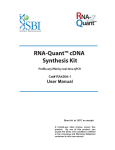
shRNA DESIGN
shRNAs, or short hairpin RNAs, are artificial constructs that can be inserted into a genome
and expressed endogenously (Paddison et al., 2002). The expressed hairpins can then fold
to form dsRNA, and Drosha and Dicer can then act on these to create mature sequence,
used by RISC complex (see Commentary) to target the genes. There are two possible
orientations of the hairpin sense-loop-antisense (SAS) or antisense-loop-sense (ASS)
shown in Figure 12.3.1, which is the design used in a library created by the Hannon Lab.
If a 29-mer is used for the hairpin as shown in the figure, then the first 22-mer from the
end is believed to be used for creating the siRNA. siRNA design considerations (see Basic
Protocol 1) are used to design 19-mers that are then extended two base pairs at the 5
end and one at the 3 end to obtain the 22-mer. This is then extended by seven base pairs
along the 5 direction to get the 29-mer. Procedures are given below for constructing the
designs, along with a concrete example to illustrate the concepts.
Let the loop sequence be TTGG, let restriction site I be EcoRI (GAATTC), and let restriction site II be SalI (GTCGAC). The U6 promoter is TTGTGGAAAGGACGAAACACC
BASIC
PROTOCOL 2
Analyzing RNA
Sequence and
Structure
12.3.3
Current Protocols in Bioinformatics
Supplement 6
U6
restriction
terminator site II
restriction
site I
U6 promoter
hairpin
x
restriction
site III
bar code
antisense
hairpin
loop
sense
Figure 12.3.1
The design of hairpins.
and the U6 terminator is TTTTT. Let the accession of interest be NM 001033, whose
current version number is 2.
NOTE: The exact restriction site and terminator and promoter sequences depend upon
the laboratory procedures involved in inserting these sequences into plasmids. Another
method of constructing these, aside from the method presented here, is to use the context
of a known miRNA. An miRNA with a target strand of length 22 is picked, and the target
sequence is replaced with the antisense strand from the design above. The complementary
strand is also replaced, taking care to preserve the bulges, loops, and other types of
mismatches. This helps ensure that the precursor sequence, generated by Drosha, is
properly and efficiently processed by the Dicer and gets associated properly with the
RISC complex.
Necessary Resources
Hardware
Any computer with at least 512 Mb of RAM (more is better) with a high-speed
Internet connection
Software
NCBI BLAST (UNITS 3.3 & 3.4), which can be downloaded from NCBI
(http://www.ncbi.nlm. nih.gov)
MySQL database (download from http://www.MySQL.com; UNIT 9.2)
Apache Web server (http://www.apache.org)
Programming language: all the work can be done using Perl (Schwartz and
Phoenix, 2001), though other languages can also be used
1. Using the procedures given for siRNA design (see Basic Protocol 1), it is found that the
19-mer CAAAGTATGGTATAAGAAA is one of the good designs for NM 001033.2.
2. Extending it 2 base pairs in the 3 direction and one in the 5 direction gives the
22-mer: GCAAAGTATGGTATAAGAAACA.
3. Extending it 7 base pairs along the 5 direction gives the 29-mer:
GAAGATTGCAAAGTATGGTATAAGAAACA.
4. Generate the antisense sequence: TGTTTCTTATACCATACTTTGCAATCTTC.
5. Create a hairpin by concatenating the antisense loop and sense strand, in that order:
TGTTTCTTATACCATACTTTGCAATCTTCTTGGGAAGATTGCAAAGTATG
GTATAAGAAACA.
RNAi: Design
and Analysis
6. Use a folding program like mfold (http://www.bioinfo.rpi.edu/applications/mfold/)
to confirm that the hairpin folds correctly. The result is shown in Figure 12.3.2.
12.3.4
Supplement 6
Current Protocols in Bioinformatics
10
20
30
U
U
GUUUCUU A U A C C A U A CUUUGC A A UCU UC
U
C A A AGA A U A UGGU A UGA A A CGUU AGA AG G
A^
G
60
Figure 12.3.2
50
40
Output from mfold for the author’s hairpin design.
7. Add a SalI site to the 5 end of the hairpin:
GTCGACTGTTTCTTATACCATACTTTGCAATCTTCTTGGGAAGATTGCAAA
GTATGGTATAAGAAACA
8. Add the U6 promoter sequence to the 5 end of the hairpin:
TTGTGGAAAGGACGAAACACCGTCGACTGTTTCTTATACCATACTTTGCA
ATCTTCTTGGGAAGATTGCAAAGTATGGTATAAGAAACA
The U6 promoter ensures that the gene gets expressed.
9. Add the U6 terminator sequence to 3 end of the hairpin:
TTGTGGAAAGGACGAAACACCGTCGACTGTTTCTTATACCATACTTTGCA
ATCTTCTTGGGAAGATTGCAAAGTATGGTATAAGAAACATTTTT.
The terminator ensures that only the hairpin gets expressed, i.e., that there is no runthrough.
10. Add an EcoRI site to the 3 end of the hairpin:
TTGTGGAAAGGACGAAACACCGTCGACTGTTTCTTATACCATACTTTGCA
ATCTTCTTGGGAAGATTGCAAAGTATGGTATAAGAAACATTTTTGAATTC.
11. Add CC to the 3 end of the hairpin for the restriction site to work:
TTGTGGAAAGGACGAAACACCGTCGACTGTTTCTTATACCATACTTTGCAA
TCTTCTTGGGAAGATTGCAAAGTATGGTATAAGAAACATTTTTGAATTCCC.
12. Make sure that only one copy of each restriction site and the U6 terminator occur in
the sequence.
13. Reverse complement the whole construct, and send it to a facility for DNA synthesis:
GGGAATTCAAAAATGTTTCTTATACCATACTTTGCAATCTTCCCAAGAAGA
TTGCAAAGTATGGTATAAGAAACAGTCGACGGTGTTTCGTCCTTTCCACAA.
14. The oligo is synthesized as a DNA, cloned into a plasmid using PCR, grown, and then
inserted into a vector. For transient effects, the plasmid can be transfected into the
cell with the effects seen about 48 hours after transfection; for permanent insertion,
the vector is used to infect the cell.
PREDICTION OF miRNA GENES
Discovery of novel miRNA genes can help with the discovery of the various subtle
features of the RNAi pathway, which in turn facilitates more rational shRNA designs.
The steps involved in predicting miRNA genes are outlined below.
BASIC
PROTOCOL 3
1. Identify regions outside coding regions that are homologous across genomes.
2. Of these regions, find ones that can form short hairpin structures (total length <100
base pairs).
Analyzing RNA
Sequence and
Structure
12.3.5
Current Protocols in Bioinformatics
Supplement 6
3. Once an miRNA is identified in a genome, it can be used to find homologous miRNAs
in related genomes.
The programs MiRscan and MiRseeker (see Internet Resources) implement the ideas in the
above steps. Cloning and sequencing small RNAs have verified several of these predictions.
They have also been used to place upper bounds on the number of miRNA genes in the
human and mouse genomes. The problem with such techniques is that they will miss
miRNAs that have diverged a lot over evolutionary time scales. For greater details the
reader is referred the original publications referenced above and encouraged to use their
Web sites for exploration of the programs.
BASIC
PROTOCOL 4
IDENTIFYING TARGETS OF miRNA
Once miRNAs can be reliably mapped to their targets, the key is provided to understanding
the nature of the targeting machinery, which is crucial to designing better si and shRNAs.
This knowledge allows assignment of biological function to the miRNA genes. This may
also allow rational design of shRNAs that have a calibrated potency, that is, the shRNAs
can silence with varying efficiencies ranging from 0% to 100% (Hemann et al., 2003).
Due to G:U wobble base pairing and matches with several loops, the number of potential targets for each miRNA is quite large. Identifying them and making sense of the
developmental pathways is a daunting task that is currently being undertaken in several
laboratories (Rhoades et al., 2002). The steps involved in prediction of miRNA targets
are outlined below
1. Identify target genes for miRNAs. The mature products of miRNA genes have been
experimentally sequenced. Using a dynamical programming approach that also allows G:U base pairing will help identify putative matches for the mature sequence.
The matches for miRNAs are usually assumed to lie in the 3 UTR, but this is not
necessarily true. It is also usually assumed that the first seven nucleotides must match
well.
2. Use homology with other species to narrow down the list of targets.
3. Use pathway information to select miRNAs that regulate related mRNAs.
ALTERNATE
PROTOCOL 1
BUILDING AND USING A LIBRARY OF shRNAs
The use of an shRNA library allows large-scale studies that are prohibitively expensive
with siRNAs. Using shRNA, it is now possible to perform genome-wide analysis in ways
that are not feasible with siRNA. A library has been constructed along these lines and is
available from the Hannon Lab at Cold Spring Harbor Laboratory (http://www.cshl.org;
Paddison et al., 2004).
Library construction requires making a collection of shRNAs that can be ordered off-theshelf. The collection needs to be fairly complete, covering every major functional group
and almost all known genes (at least the major variants of each gene type). In addition,
the collection needs to contain constructs that can be trusted to work. This is required,
since it is impossible to have functional assays for each individual construct. Instead, the
library is most likely to be used for silencing collections of genes in functional groups,
such as kinases. Building the library involves the steps outlined below.
Necessary Resources
Hardware
RNAi: Design
and Analysis
Any computer with at least 512 Mb of RAM (more is better) with a high-speed
Internet connection
12.3.6
Supplement 6
Current Protocols in Bioinformatics
Software
NCBI BLAST (UNITS 3.3 & 3.4), which can be downloaded from NCBI
(http://www.ncbi.nlm.nih.gov)
MySQL database (download from http://www.MySQL.com; UNIT 9.2)
Apache Web server (http://www.apache.org)
Programming language: all the work can be done using PERL, though other
languages can also be used
Build the library
1. Design at least three shRNAs per gene (see Basic Protocol 2). All of the design
principles for siRNAs apply (see Basic Protocol 1). In addition, one can pick oligos
that can work for both mouse and human genes (this has indeed been done for the
library at CSHL), allowing use of common oligos in both species.
2. Barcodes (random 60-mer sequences synthesized in a lab; Paddison et al., 2004) are
inserted into the construct.
The barcode at the end is a random 60-mer that is unique to each hairpin allowing
identification of the hairpin, either via microarrays, as described below, or via the use of
PCR.
3. Set up a laboratory tracking system (LIMS) and make data accessible through a Webbased access system. All the data can be put into a MySQL database, and a Web
interface can be set up, using an Apache server, along with CGI scripts.
This step is crucial as it allows Web-based access to the data for bench scientists. The
details can be found in many books (Lee and Ware, 2002), and will not be provided here.
4. The shRNAs must be verified by sequencing, before use. Use a MySQL database
(UNIT 9.2) to track the fate of the sequencing activities.
5. Build a BLAST database (UNITS 3.3, 3.4 & 3.11) of all the target sequences in the library, so
users can input names and get back oligos against their genes. This removes problems,
e.g., with annotations or errors in naming.
6. Keep track of the barcodes for each construct, as these are crucial for analysis of
assays.
Use the library
7. Design the study using the annotation of the genes. For example, to design a study
on the effect of kinases on cancer cells, find all the shRNAs that silence kinases and
get them from the library.
8. The list of shRNAs will form the pool of oligos that can be obtained from the laboratories that have constructed the libraries (the library from the Hannon Lab mentioned
above is one of several that have been constructed; Berns et al., 2004; Paddison et al.,
2004). Transfected or infect the relevant shRNAs into cells, at a dilution that ensures
statistically that there will be one shRNA per cell.
9. Grow the cells for a few generations.
10. Extract the shRNAs from the cells using restriction enzymes. Microarrays designed
to detect the barcodes are used to find shRNAs that have been depleted. Analysis of
microarray data is done using either custom-made or ready-made software, details of
which are discussed elsewhere in this manual (see Chapter 7).
Analyzing RNA
Sequence and
Structure
12.3.7
Current Protocols in Bioinformatics
Supplement 6
11. Find the mRNAs that are targets of the shRNAs that have been depleted and design
further studies using other techniques (these techniques depend on the biological
questions being addressed and are outside the scope of this unit).
COMMENTARY
Background Information
RNAi: Design
and Analysis
Biological premise of RNAi
RNAi is a powerful new technique that
promises to revolutionize the study of gene
function and genetic networks by enabling relatively easy and selective silencing of genes.
Efficient use of RNAi requires a good understanding of the mechanism in order to build
better silencing constructs and construct libraries of silencing constructs. This unit provides a survey of methods used in various
stages of the process as well as the details
of designs of RNAi oligos (either siRNA or
shRNA). Figure 12.3.3 shows how RNAiinduced silencing works in vivo. Drosha, a ribonuclease III (RnaseIII) enzyme, processes
dsRNA in the nucleus. The Drosha product, a
dsRNA, is then exported to the cytoplasm by a
factor called exportin-5. In the cytoplasm, another RNaseIII enzyme, Dicer, cuts the dsRNA
into short interfering RNAs, (siRNA), which
are 22- to 29-nucleotide (nt) double-stranded
RNAs with a 2-nt overhang at the 3 end of
each strand. The RNA Interference Silencing
Complex (RISC) uses a single strand of the
siRNA to target genes for silencing by message
degradation. RISC consists of Argonaute (1
and 2), Fragile X related protein (FXRP), Vasa
Intronic Gene (VIG), and other factors, Understanding the physical process at each of these
steps can help in the design of more specific
and potent siRNAs (Denli and Hannon, 2003).
In plants and animals, short (∼22nt) noncoding RNAs, called microRNAs
(miRNAs), are involved in developmental
pathways through regulation of protein expression, either through message degradation or by
translational repression (Bartel, 2004). miRNAs use at least part of the RNAi pathway,
but usually end up blocking translation, rather
than degrading the message. A better understanding of miRNAs will lead to better use of
RNAi as a tool for biological investigations.
One artificial method of harnessing RNAi
to silence genes is to introduce siRNAs into
a cell, going directly to the RISC processing
step (Elbashir et al., 2001). This is a common
laboratory technique now; design of siRNAs
is discussed in Basic Protocol 1.
Another artificial method of introducing
dsRNA into the cell is to insert hairpin
constructs into the genome of the host cell and
get them expressed endogenously (Paddison
et al., 2002). This ensures stable suppression,
and can be made inducible—i.e., the expression of the dsRNA can be controlled by external factors such as drugs. In mammalian
cells, introducing large dsRNA can result in
an interferon response that leads to cell death.
Thus, the dsRNA has to be short. The details
of the design process are described in Basic
Protocol 2.
Study of proteins involved in RNAi
The study of protein families involved in
RNAi can help reveal new members of these
families and uncover new mechanisms of the
pathway. This, in turn, can help with designing
shRNAs and siRNAs with degree of silencing
specified by the user (Hemann, et al., 2003).
This is an active area of research, especially as
more genomes are being sequenced (Carmell
et al., 2002).
Conserved domains in RNAi-related proteins are identified and then used to identify other proteins that might be involved in
the pathway. Here, the authors briefly discuss the study of RnaseIII enzymes. There
are three classes of RnaseIII enzymes; the
first class (E. coli) contains one catalytic
endonuclease domain (RIII domain), and a
dsRNA-binding domain (dsRBD). The second class (Drosha) has two RIII domains,
and the third class (Dicer) usually contains
a DexH-box helicase domain, two RIII domains, a PAZ domain, and a dsRBD domain.
The PAZ domain is a characteristic feature of
the Argonaute family of proteins, which also
contain a PIWI domain. The helicase domain
unwinds double stranded RNA, and the PAZ
domain is believed to bind to single stranded
RNA.
The steps involved in this kind of discovery
are outlined below.
1. Align the domains from the known proteins to get a multiple alignment, using programs such as ClustalW (UNIT 2.3) or T-Coffee
(UNIT 3.8) for each domain of interest (see Internet Resources for the Web sites of these programs).
2. Build an HMM (see Internet Resources
for S.R. Eddy’s HMMER Web site) from this
alignment for each domain.
12.3.8
Supplement 6
Current Protocols in Bioinformatics
nucleus
cytoplasm
Drosha
Dicer
rtin
po
ex
siRNAs
Dicer
Ago complexes
translational
inhibition
mRNA cleavage
degradation
(RISC)
Ago:
MNT
FXR
VIG
Figure 12.3.3 The processes involved in RNAi. Abbreviations: MNT, micrococcal nuclease tudor;
FXR, fragile X–related; VIG, vasa intronic gene.
3. Search the protein database to identify
proteins with the domains (e.g., UNITS 2.2, 2.4
& 2.5).
4. Identify the proteins in the various classes
and try to assign function. The multiple alignments built above can be used to study the
phylogeny of these families. The study of the
phylogeny of the complexes involved in the
pathway provides information on the evolution of the pathway and may even help identify novel conserved domains. The interested
reader is referred to other relevant units of this
manual for more information on the procedures used here.
5. Carry out a phylogenetic analysis to understand the evolution of these proteins (see
Chapter 6).
Acknowledgments
Greg Hannon, Doug Conklin, and JoseMaria Silva taught me all I know about RNAi.
Ahmet Denli helped with the figures. Marco
Mangone, Susan Janicki, Jose-Maria Silva,
and Xavier Roca read the manuscript critically.
Literature Cited
Bartel, D.P. 2004. MicroRNAs: Genomics, biogenesis, mechanism, and function. Cell 116:281-297.
Berns, K., Hijmans, E.M., Mullenders, J., Brummelkamp, T.R., Velds, A., Heimerikx, M.,
Kerkhoven, R.M., Madiredjo, M., Nijkamp, W.,
Weigelt, B., Agami, R., Ge, W., Cavet, G., Linsley, P.S., Beijersbergen, R.L., and Bernards, R.
2004. A large-scale RNAi screen in human cells
identifies new components of the p53 pathway.
Nature 428:431-437.
Analyzing RNA
Sequence and
Structure
12.3.9
Current Protocols in Bioinformatics
Supplement 6
Carmell, M.A., Xuan, Z., Zhang, M.Q., and Hannon, G.J. 2002. The Argonaute family: Tentacles that reach into RNAi, developmental control, stem cell maintenance, and tumorigenesis.
Genes Dev. 16:2733-2742.
Denli, A.M. and G.J. Hannon 2003. RNAi: An evergrowing puzzle. Trends Biochem. Sci. 28:196201.
Elbashir, S.M., Harborth, J., Lendeckel, W., Yalcin,
A., Weber, K., and Tuschl, T. 2001. Duplexes of
21-nucleotide RNAs mediate RNA interference
in cultured mammalian cells. Nature 411:494498.
Hannon, G.J. 2002. RNA interference. Nature
418:244-251.
Internet Resources
http://www.ambion.com/catalog/supp/
silencer lib.html
Ambion company Web site.
http://www.apache.org
Apache open source Web server.
http://www.ebi.ac.uk/clustalw/
ClustalW: Open source multiple alignment program..
http://katahdin.cshl.org:9331/siRNA
Cold Spring Harbor Laboratory siRNA Web site (R.
Sachidanandam and J. Lee).
http://www.dharmacon.com/
Hemann, M.T., Fridman, J.S., Zilfou, J.T., Hernando, E., Paddison, P.J., Cordon-Cardo, C.,
Hannon, G.J., and Lowe, S.W. 2003. An epiallelic series of p53 hypomorphs created by stable RNAi produces distinct tumor phenotypes in
vivo. Nat. Genet. 33:396-400.
Dharmacon company Web site.
Khvorova, A., Reynolds, A., and Jayasena, S.D..
2003. Functional siRNAs and miRNAs exhibit
strand bias. Cell 115:209-216.
Hannon Laboratory Web site at Cold Spring Harbor
Laboratory.
Lee, J.B. and Warc, B. 2002. Open Source Web Development with LAMP: Using Linux, Apache,
MySQL, Perl, and PHP. Addison-Wesley, Reading, Mass.
HMMER Web site (S.R. Eddy). Open source HMM
tools.
Paddison, P.J., Caudy, A.A., Bernstein, E., Hannon, G.J., and Conklin D.S. 2002. Short hairpin
RNAs (shRNAs) induce sequence-specific silencing in mammalian cells. Genes Dev. 16:948958.
Paddison, P.J., Silva, J.M., Conklin, D.S.,
Schlabach, M., Li, M., Aruleba, S., Balija,
V., O’Shaughnessy, A., Gnoj, L., Scobie,
K., Chang, K., Westbrook, T., Cleary, M.,
Sachidanandam, R., McCombie, W.R., Elledge,
S.J., and Hannon, G.J. 2004. A resource for
large-scale RNA-interference-based screens in
mammals. Nature 428:427-431.
Rhoades, M.W., Reinhart, B.J., Lim, L.P., Burge,
C.B., Bartel, B., and Bartel, D.P. 2002. Prediction of plant microRNA targets. Cell 110:513520.
Schwartz, R.L. and Phoenix, T. 2001. Learning Perl.
O’Reilly & Associates, Sebastopol, Calif.
Schwarz, D.S., Hutvagner, G., Du, T., Xu, Z.,
Aronin, N., and Zamore, P.D. 2003. Asymmetry
in the assembly of the RNAi enzyme complex.
Cell 115:199-208.
http://design.dharmacon.com/rnadesign/default.
aspx?sid=731615029
Dharmacon siRNA Design Center.
http://www.cshl.org/public/SCIENCE/hannon.html
http://hmmer.wustl.edu/
http://www.bioinfo.rpi.edu/applications/mfold/
mfold: Open source RNA folding program (M.
Zuker).
http://genes.mit.edu/mirscan/
MiRscan Web site (M. Mawson, L.P. Lim, and N.
Lau).
http://toy.lbl.gov:9050/cgi-bin/miRseeker.pl
MiRseeker Web site (P. Tomancak).
http://www.mysql.com
MySQL: Open source database.
http://www.ncbi.nlm.nih.gov/
NCBI: A site for genomics data, tools, and analyses.
http://igs-server.cnrs-mrs.fr/Tcoffee/
T-Coffee server.
Contributed by Ravi Sachidanandam
Sachidanandam Lab
Cold Spring Harbor Laboratory
Cold Spring Harbor, New York
RNAi: Design
and Analysis
12.3.10
Supplement 6
Current Protocols in Bioinformatics
Predicting the Secondary Structure
Common to Two RNA Sequences with
Dynalign
UNIT 12.4
Dynalign is an algorithm that uses dynamic programming to simultaneously find the
lowest free energy secondary structure common to two RNA sequences and the sequence
alignment that facilitates that structure (Mathews and Turner, 2002a). By using two
sequences, the accuracy of secondary structure prediction is improved as compared to
free energy minimization structure prediction of a single sequence. For example, with a
database of 5S RNA sequences poorly predicted by free energy minimization of a single
sequence, the average accuracy of prediction improved from 47.8% to 86.4% with the
use of two sequences (Mathews and Turner, 2002a).
This unit presents two protocols for using Dynalign. The Basic Protocol covers the
use of Dynalign with the RNAstructure program in Microsoft Windows. The Alternate
Protocol covers the compilation and use of Dynalign on a Unix or Linux operating system.
Selection of sequences and choice of basic parameters used by Dynalign are discussed
in Background Information.
USING DYNALIGN ON A WINDOWS PLATFORM WITH RNAstructure
This protocol details step-by-step instructions for the use of the Dynalign algorithm on
Windows using the program RNAstructure. It assumes some basic familiarity with the
Microsoft Windows operating system. An example is drawn from two tRNA sequences,
RA7680 and RD0260, derived from the Sprinzl database (Sprinzl et al., 1998).
BASIC
PROTOCOL
Necessary Resources
Hardware
RNAstructure runs under Microsoft Windows, including Windows ME, Windows
NT, Windows 2000, and Windows XP. Dynalign will support any hardware
configuration; however, see Background Information to consider the possible
time and memory requirements for sequences of interest.
RNAstructure is also known to run stably on Linux using Wine (http://www.
winehq.com), a Windows emulator. It has been tested on Wine, version
December 12, 2003, under RedHat Linux 9. Detailed instructions for installing
RNAstructure on Linux are beyond the scope of this unit, although the use of the
program is identical under both Windows and Linux.
Software
The software package, RNAstructure, can be downloaded from the World Wide
Web at http://rna.chem.rochester.edu/RNAstructure.html. Registration is required
for download, so that a count of those using the software can be maintained and
so users can be notified of significant updates in the software. The list of
registered users is not shared with others and not used for any other purpose.
Files
Text files of the RNA sequences of interest, in their 5 to 3 orientation. The
sequence file format, .seq, required by Dynalign is illustrated in Figure 12.4.1.
Contributed by David Mathews
Current Protocols in Bioinformatics (2004) 12.4.1-12.4.11
C 2004 by John Wiley & Sons, Inc.
Copyright Analyzing RNA
Sequence and
Structure
12.4.1
Supplement 8
Figure 12.4.1 A Sample Sequence (.seq)
file. Any number of comment lines, labeled with
a semicolon, can precede the sequence. The required title is on the next line and must be contained on a single line. The sequence follows,
listed from 5 to 3 . White space is ignored, but
the sequence must terminate with 1. Note that
RNAstructure and Dynalign do not allow lowercase nucleotides to base-pair; therefore most
nucleotides must be entered in uppercase.
In Windows, it is generally easier to enter the sequence in the sequence editor,
which uses this format to save the files. In Unix/Linux (see Alternate Protocol),
the sequence file format must be explicitly entered. Note that the sequence
should generally be entered in uppercase, because lowercase nucleotides are
forced to be single-stranded in structure predictions. Also note that when RNA
thermodynamic parameters are used for structure prediction, nucleotides entered
as T are treated as uracil in structure predictions. The symbol X can be used for
nucleotides that do not stack or base-pair.
Download and install RNAstructure
1. Download RNAstructure as RNAstructure.zip from http://rna.chem.rochester.
edu/RNAstructure.html.
2a. For versions of Windows other than Windows XP: RNAstructure.zip needs
to be uncompressed before installation using a decompression program such
as WinRAR (http://www.rarlab.com), WinZip (http://www.winzip.com), or PKZIP
(http://www.pkware.com). Using one of these tools, uncompress the contents of
RNAstructure.zip to a temporary folder, then double-click on SETUP.exe.
2b. For Windows XP: Double-click on RNAstructure.zip to open the compressed
folder, then double-click SETUP.exe to install.
SETUP.exe will carry out all the steps required for Windows installation. The user can
choose to override the default destination directory and default name for the program in
the Windows Start Menu.
Enter the sequences
3. If the default menu item was chosen, start RNAstructure by choosing RNAstructure
from the RNAstructure 4 item in the Windows Start Menu.
4. To enter sequences in RNAstructure, use the sequence editor, which can be opened
either by selecting New Sequence from the File menu or by clicking the New Sequence icon at the far left of the toolbar. The sequence editor will open as shown in
Figure 12.4.2.
Note that items in the toolbar, located directly under the menu bar, identify themselves
with a pop-up label if the mouse pointer is placed over that icon.
5. Enter a title in the Title field at the top. This title will be used to label the output from
calculations. The Comment field provides an opportunity to save comments with the
sequence. Finally, enter the sequence, from 5 to 3 , in the Sequence field.
Predicting RNA
Secondary
Structure with
Dynalign
Sequences can be entered by hand or pasted from other programs by cut and paste. A
sequence copied to the clipboard can be pasted into the Sequence field by first clicking in
the Sequence field to place the cursor and then choosing Paste from the Edit menu item
or typing Ctrl-V.
12.4.2
Supplement 8
Current Protocols in Bioinformatics
Figure 12.4.2
The RNAstructure sequence editor.
Several tools are available in the sequence editor. Clicking the Format Sequence button
places the sequence in columns of five nucleotides with fifty nucleotides per line. If the Read
Sequence button is clicked, the sequence is read aloud (over the computer’s speakers) from
5 to 3 . This can be canceled by clicking the same button, which has its label changed to
Cancel Read. Also, the sequence can be read while it is typed by choosing Read Sequence
While Typing on the Read menu item. The secondary structure can be predicted for a
single sequence by clicking Fold as RNA or Fold as DNA buttons. Protocols for secondary
structure prediction for a single sequence using RNAstructure are detailed elsewhere
(Mathews et al., 2000).
6. Save the sequence either by choosing Save Sequence under the File menu item or by
clicking the disk icon on the toolbar. This sequence can later be accessed by opening
the file with the sequence editor, either by choosing Open Sequence under the File
menu item or by clicking the Open Sequence icon on the toolbar.
The two sequences for the sample calculation, RA7680 and RD0260, are included with
RNAstructure, so they do not need to be entered.
Starting Dynalign
7. After both sequences have been entered and saved using the sequence editor, proceed
to the Dynalign window by choosing Dynalign under the File menu item or by clicking
the Dynalign icon on the toolbar. Figure 12.4.3 illustrates the Dynalign window.
8. Choose the first sequence by clicking the button labeled Sequence File 1. The standard
Windows File Open Dialog box will appear for selecting the sequence. For example,
open RA7680.seq from the RNAstructure installation folder. Repeat this for the
second sequence by clicking the Sequence File 2 button, and select RD0260.seq.
The shorter of the two sequences should always be used as sequence 1 to save
calculation time.
Analyzing RNA
Sequence and
Structure
12.4.3
Current Protocols in Bioinformatics
Supplement 8
Figure 12.4.3 The Dynalign window in RNAstructure. Two tRNA sequences that are included
with RNAstructure are selected and the default parameters are shown. The calculation is started
by clicking the START button.
9. Default values will now be displayed for the user-adjustable parameters and for
the output files. The predicted structures will be output in CT files (see Guidelines
for Understanding Results) and the predicted alignment is output in plain text. The
names of these files can be changed from the default by clicking the buttons labeled
CT File 1, CT File 2, or Alignment File. The values for M and Gap Penalty can be
adjusted (see Critical Parameters).
For the example calculation, use the default values for M (15) and gap penalty (0.4).
Finally, to allow single-base-pair inserts in the structures, the check box after Single BP
Inserts Allowed should be checked.
10. Begin the calculation by clicking the START button. A window labeled Dynalign in
Progress, with a progress bar, will open to show the progress of the calculation. The
calculation may take some time. Refer to Background Information, which contains
a table for sample calculation times.
Viewing the output
11. When the Dynalign calculation is complete, a dialog box appears that gives the options
of “draw structures” and “cancel.” Click the “draw structures” button to display
the structures on the screen. This opens the interactive drawing tool incorporated
in RNAstructure. The structure of each of the two sequences is drawn in a separate
window. Figure 12.4.4 shows the structure for the RA7680 tRNA sequence, predicted
using Dynalign.
Predicting RNA
Secondary
Structure with
Dynalign
12. To zoom in and out of the structure, use the Ctrl–right arrow and Ctrl–left arrow
keys. Alternatively, the zoom level can be chosen by clicking Zoom under the Draw
menu item. The structure can be drawn clockwise or counterclockwise by checking
or unchecking Render Clockwise, respectively, under the Draw menu.
12.4.4
Supplement 8
Current Protocols in Bioinformatics
Figure 12.4.4 Sample output from the Dynalign algorithm. This is the secondary structure predicted for the tRNA sequence RA7680.
13. The sequence alignment is saved as a plain text file with the extension .ali. It can be
viewed with any text editor, such as WordPad, which comes with Windows. To view
this file, double-click on the file in Windows Explorer or in the folder in which it was
saved.
If an .ali file has never been opened on the computer, Windows will ask which program
to use to open the file. Choose WordPad from the list of programs and click the check
box next to “Always use this program to open this type of file” so that the next .ali
file will be opened by Wordpad. Note that in Windows XP, after double-clicking the file,
Windows will query whether to “Use the Web service to find the appropriate program”
or “Select the program from a list.” Choose “Select the program from a list” to proceed
to the program list. The file format for alignments is explained below (see Guidelines for
Understanding Results).
Getting help with RNAstructure
14. RNAstructure includes online help, available by clicking Help Topics under the Help
menu item. The online help is organized into chapters covering the different functions.
An index is also available by clicking the index button from the online help window.
USING DYNALIGN FOR UNIX/LINUX
This protocol details the use of Dynalign on Unix/Linux, including local compilation.
A sample calculation is run using two tRNA sequences as an example. Basic familiarity
with Unix is required (see APPENDIX 1C).
Alternatively, the RNAstructure package for Windows can be installed on the Linux operating system using the Windows emulator, Wine, as in the Basic Protocol. RNAstructure
is known to run stably on Wine, version December 12, 2003, with RedHat Linux 9. RNAstructure is described above in the Basic Protocol and comes with an install program and
online help.
ALTERNATE
PROTOCOL
Analyzing RNA
Sequence and
Structure
12.4.5
Current Protocols in Bioinformatics
Supplement 8
Necessary Resources
Hardware
Dynalign will run on any machine using Unix or Linux. See Background
Information for sample computation times and memory requirements.
Software
Dynalign for Unix/Linux is available for download from the World Wide Web at
http://rna.chem.rochester.edu/dynalign.html. A C++ compiler will be needed
compile the program. To display an automated drawing of the Dynalign output, a
secondary structure drawing package is required. On such package is Naview
(Bruccoleri and Heinrich, 1988), which has been modified by Darren Stuart and
Michael Zuker and is available for download at http://www.bioinfo.rpi.edu/
∼zukerm/rna/node3.html#SECTION00033.
Files
Text files of the RNA sequences of interest. Sequences are required to be in the
.seq format, detailed in the Necessary Resources section of the Basic Protocol
(Fig. 12.4.1). Two sample tRNA sequences are included in dynalign.tar.
Install Dynalign
1. Extract the contents of Dynalign.tar, for example with:
tar -xvf Dynalign.tar
The directory dynalign will be created, which contains the source code, the
thermodynamic parameter files, a Makefile, a ReadMe.txt file, and two sample
tRNA sequences, RA7680.seq and RD0260.seq (Sprinzl et al., 1998). The
ReadMe file contains some instructions for installing and using Dynalign.
2. To compile Dynalign, first edit the Makefile to indicate the name of the local
compiler. The default is the GNU compiler, g++. Two other compiler names are
suggested, CC for Sun Solaris or SGI IRIX, and icc for the Intel C++ compiler.
3. Next enter the following command at the shell prompt to compile the program:
make dynalign
The executable, dynalign, and thermodynamic parameter files (*.dat files) can be
moved to any location.
4. Finally, define the environment variable DATAPATH to indicate the location of the
thermodynamic data files. Dynalign reads the data files with each execution to define
the free energy parameters (Mathews et al., 1999; Mathews and Turner, 2002b). For
example, in bash, use the command:
export DATAPATH=/usr/local/dynalign/
or, in csh, use the command:
setenv DATAPATH /usr/local/dynalign/
where the local path should be substituted for /usr/local/dynalign/. The
final slash must be included.
Predicting RNA
Secondary
Structure with
Dynalign
12.4.6
Supplement 8
Current Protocols in Bioinformatics
Figure 12.4.5 Dynalign input. User-provided responses are shown in bold for clarity. This input
will predict the common secondary structure and alignment for the two tRNA sequences, RA7680
and RD0260.
Running Dynalign
5. Start Dynalign by using the following command (assuming that Dynalign is in the
user path):
dynalign
Figure 12.4.5 shows the user input required to find the structure common to the
two tRNA sequences, RA7680 and RD0260, and the alignment of the sequences.
The user specifies the names of each sequence, the max separation, the gap penalty,
whether single-base-pair inserts are allowed (where 1 means allow single base pair
inserts), and the names of output files. The max separation is the M parameter (see
Critical Parameters). The gap penalty penalizes gaps inserted into the sequence
alignment; 0.4 is a good starting point for calculations. After the information is
entered, Dynalign will start the calculation.
Plain text is output to indicate the progress of the calculation.
6. Dynalign outputs a CT file for each sequence that specifies the base pairing of each
nucleotide. This file is explained in Guidelines for Understanding Results, below. A
plain text alignment file, also explained in Guidelines for Understanding Results, is
also output. Figure 12.4.4 illustrates the predicted secondary structure of one of the
two tRNA sequences used for this example, drawn with RNAstructure (see Necessary
Resources for this protocol; also see Basic Protocol).
GUIDELINES FOR UNDERSTANDING RESULTS
Three output files are generated by Dynalign, the CT files, which contain predicted base
pairs for a single sequence, and the alignment file, which contains the predicted alignment
of the two sequences. The Dynalign sequence alignment is output in plain text and the
format is illustrated in Figure 12.4.6 using the example of the two tRNA sequences,
RA7680 and RD0260, derived from the Sprinzl database (Sprinzl et al., 1998). The CT
file containing the base pairs predicted for RA7680 is shown in Figure 12.4.7.
Analyzing RNA
Sequence and
Structure
12.4.7
Current Protocols in Bioinformatics
Supplement 8
Figure 12.4.6 Sample alignment (.ali) file. This is the alignment predicted for two tRNA sequences, RA7680 and
RD0260, with RA7680 on top. The score reported is the Gtotal (Equation 12.4.1). Inserts are represented by a dash (–),
and the caret symbols show locations of base pairs.
Predicting RNA
Secondary
Structure with
Dynalign
Figure 12.4.7 A sample CT file. The structure predicted for RA7680 is shown (for graphic equivalent, see Fig. 12.4.4), with nucleotides 20 through 60 omitted for brevity. The first line gives a count
of nucleotides, followed by the sequence title. Each nucleotide is then represented by a single line.
From left to right are the nucleotide position, nucleotide type, 5 connected nucleotide, 3 connected
nucleotide, canonical pair, and historical numbering. A break in the 5 connected nucleotide and 3
connected nucleotide sequence can be used to indicate separate strands, although Dynalign does
not use this functionality. A 0 in the canonical pair column indicates that the nucleotide is unpaired.
Note the symmetry in the canonical pair column—e.g., nucleotide 2 is paired to 71 and 71 is paired
to 2. Historical numbering can be used to annotate a structure with a natural numbering scheme;
for example, if the sequence was extracted from a longer sequence, the natural numbering does
not need to start with 1. Dynalign will always output historical numbering identical to nucleotide
position.
12.4.8
Supplement 8
Current Protocols in Bioinformatics
COMMENTARY
Background Information
The prediction of RNA secondary structure
has been shown to be about 73% accurate at
predicting base pairs for a diverse database of
secondary structures (Mathews et al., 2004).
This accuracy can be improved by constraining prediction with the use of experimental
constraints (Mathews et al., 1999; 2004) such
as enzymatic (Knapp, 1989) or FMN cleavage
(Burgstaller and Famulok, 1997), or chemical
modification data (Ehresmann et al., 1987). Alternatively, the accuracy of secondary structure
prediction can be improved by taking advantage of information contained in sequence evolution by using multiple sequences.
Methods for using multiple sequences to
predict structures are divided into two groups:
those that use a fixed alignment (Corpet
and Michot, 1994; Juan and Wilson, 1999;
Knudsen and Hein, 1999; Lück et al., 1999;
Hofacker et al., 2002) and those that simultaneously find the sequence alignment and secondary structure (Sankoff, 1985; Eddy and
Durbin, 1994; Gorodkin et al., 1997; Chen
et al., 2000; Holmes and Rubin, 2002; Mathews and Turner, 2002a). In general, methods
that use a fixed alignment are not as robust
because the alignment is determined by sequence matching using ClutsalW (UNIT 2.3;
Thompson et al., 1994) or similar methods (see
UNIT 3.7). Compensating base-pair changes (the
change of two nucleotides in a sequence that
preserves a conserved base pair) are required
proof for the existence of helices (Pace et al.,
1999). These compensating changes, however,
frustrate methods for determining alignments
based on sequence matching alone. Methods that simultaneously determine the common secondary structure and alignment, on
the other hand, although more robust, can take
considerably more time to execute.
ondary structure and alignment of the two sequences is then found, such that each base pair
in the common secondary structure must be accommodated by the sequence alignment. The
total free energy minimized is defined as:
Equation 12.4.1
where Ggap is a parameter that calibrates the
cost of introducing gaps in the sequence alignment to the Gibbs free energy of secondary
structure formation in RNA. Conformational
free energies for each sequence are predicted
using the nearest-neighbor parameters derived
by Doug Turner and co-workers (Xia et al.,
1998; Mathews et al., 1999, 2004).
To reduce the time and storage cost of the
algorithm, the set of possible alignments is reduced using a parameter, M. This parameter
limits the alignment so that for nucleotide i in
sequence A to align to nucleotide j in sequence
B, |i – j| ≤ M. This limitation makes intuitive
sense because nucleotides with very different
positions in each sequence are unlikely to be
aligned. An extreme example of this is that the
first nucleotide in sequence A cannot reasonably align with the last nucleotide in sequence
B. M places an upper bound on this distance.
The Dynalign algorithm is O(N3 M3 ) in time
and O(N2 M2 ) in storage, where N is the length
of the shorter sequence. This means that a doubling in either N or M results in a calculation
that takes eight times as much computer time
and four times the memory usage. Table 12.4.1
shows the calculation time for three sets of
RNA sequences ranging in length from 76 to
217 nucleotides.
Critical Parameters
The Dynalign algorithm
Dynalign is a dynamic programming algorithm based on the algorithm first suggested
by Sankoff (1985). It simultaneously predicts
the lowest free energy secondary structure for
two sequences and the alignment of the two
sequences. By using dynamic programming, it
can guarantee that the lowest free energy solution to Equation 12.4.1, below, is found, given
that the algorithm cannot predict pseudoknotted base pairs.
As input, Dynalign accepts two sequences
that are assumed to have a common secondary
structure. A lowest free energy common sec-
The user selects values for three adjustable
parameters in the calculation; M, Ggap , and
whether or not single-base-pair inserts are allowed in one of the two sequences. The choice
of M is crucial for the calculation. M must be
large enough to allow the optimal alignment,
but must also kept small to reduce the cost of
the calculation. M should be no smaller than
the difference in length of the two sequences,
and in most cases should be larger. In general,
the size of M needs to be determined by an
intuition about the alignment that will emerge
from the calculation. One method to support
a choice of M is to use Dynalign to predict
Analyzing RNA
Sequence and
Structure
12.4.9
Current Protocols in Bioinformatics
Supplement 8
Table 12.4.1 Benchmarks for Dynalign Calculation Timea
Sequence type
Sequence 1
Sequence 2
N
M
Time
(hr:min:sec)
Memory
(Mb)
tRNA
RA7680
RD0260
76
15
0:08:39
19
5S rRNA
H. volcanii
A. globiformis
122
15
0:37:09
40
D. takahashii
D. melanogaster
217
24
11:04:05
252
R2 3 UTR
a Three sets of sequences are benchmarked, where N is the length of sequence 1. Time and memory use are reported for
a 3.06 GHz Pentium 4 machine with 512 Mb RAM, using Red Hat Linux 9 and the GNU C++ compiler, version 3.2.2.
the common secondary structure and then to
repeat the calculation with a larger M, maybe
10% to 20% larger, to verify that the same common structure is found. If different structures
and alignments are predicted with a larger M, it
may be helpful to continue increasing M with
successive calculations.
Ggap has been calibrated by optimizing
the accuracy of pairwise secondary structure
predictions for 5S rRNA. The optimum value
found by this method is 0.4 kcal/mol/gap, and
this value should suffice for most calculations.
Larger values reduce the number of gaps permitted in the sequence alignment, and smaller
values permit a larger number of gaps.
The final user-specified parameter is
whether to allow single-base-pair inserts in one
sequence. In many cases, equivalent helices
can be expanded in a structural RNA of one
species compared to another. Dynalign can accommodate this by allowing single-base-pair
inserts in the structure predicted for one of
the sequences if there are conserved flanking
base pairs occurring in each strand direction. In
practice, this means that a helix of length L in
one sequence could be represented by a helix of
length as long as 2L – 1 in the other sequence.
For most Dynalign calculations, single-basepair inserts should be allowed.
Suggestions for Further Analysis
To make publication-quality secondary
structures, the program XRNA is quite
useful. It is available from the University
of California at Santa Cruz RNA Center at
http://rna.ucsc.edu/rnacenter/xrna/xrna.html.
It uses the Sun Java Runtime Environment,
which is available for most platforms,
including Linux and Windows.
Predicting RNA
Secondary
Structure with
Dynalign
Burgstaller, P. and Famulok, M. 1997. Flavindependent photocleavage of RNA at G U base
pairs. J. Am. Chem. Soc. 119:1137-1138.
Chen, J., Le, S., and Maizel, J.V. 2000. Prediction
of common secondary structures of RNAs: A
genetic algorithm approach. Nucleic Acids Res.
28:991-999.
Corpet, F. and Michot, B. 1994. RNAlign program:
Alignment of RNA sequences using both primary and secondary structures. Comput. Appl.
Biosci. 10:389-399.
Eddy, S.R. and Durbin, R. 1994. RNA sequence
analysis using covariance models. Nucleic Acids
Res. 22:2079-2088.
Ehresmann, C., Baudin, F., Mougel, M., Romby,
P., Ebel, J., and Ehresmann, B. 1987. Probing
the structure of RNAs in solution. Nucleic Acids
Res. 15:9109-9128.
Gorodkin, J., Heyer, L.J., and Stormo, G.D. 1997.
Finding the most significant common sequence
and structure in a set of RNA sequences. Nucleic
Acids Res. 25:3724-3732.
Hofacker, I.L., Fekete, M., and Stadler, P.F. 2002.
Secondary structure prediction for aligned RNA
sequences. J. Mol. Biol. 319:1059-1066.
Holmes, I. and Rubin, G.M. 2002. Pairwise RNA
structure comparison using stochastic contextfree grammars. In Proceedings of the 7th Pacific Symposium on Biocomputing (PSB 2002),
Lihue, Hawaii, January 3-7, 2002 pp. 163-174.
World Scientific Press, Singapore.
Juan, V. and Wilson, C. 1999. RNA secondary structure prediction based on free energy and phylogenetic analysis. J. Mol. Biol. 289:935-947.
Knapp, G. 1989. Enzymatic approaches to probing
RNA secondary and tertiary structure. Methods
Enzymol. 180:192-212.
Knudsen, B. and Hein, J.J. 1999. Using stochastic
context free grammars and molecular evolution
to predict RNA secondary structure. Bioinformatics 15:446-454.
Literature Cited
Lück, R., Gräf, S., and Steger, G. 1999. ConStruct:
A tool for thermodynamic controlled prediction
of conserved secondary structure. Nucleic Acids
Res. 27:4208-4217.
Bruccoleri, R.E. and Heinrich, H. 1988. An improved algorithm for nucleic acid secondary
structure display. Comput. Appl. Biosci. 4:167173.
Mathews, D.H. and Turner, D.H. 2002a. Dynalign:
An algorithm for finding the secondary structure
common to two RNA sequences. J. Mol. Biol.
317:191-203.
12.4.10
Supplement 8
Current Protocols in Bioinformatics
Mathews, D.H. and Turner, D.H. 2002b. Use of
chemical modification to elucidate RNA folding
pathways. In Current Protocols in Nucleic Acid
Chemistry (S.L. Beaucage, D.E. Bergstrum,
G.D. Glick, and R.A. Jones, eds.) pp. 11.9.111.9.4. John Wiley & Sons, Hoboken, N.J.
Mathews, D.H., Sabina, J., Zuker, M., and Turner,
D.H. 1999. Expanded sequence dependence of
thermodynamic parameters provides improved
prediction of RNA secondary structure. J. Mol.
Biol. 288:911-940.
Mathews, D.H., Turner, D.H., and Zuker, M. 2000.
RNA secondary structure prediction. In Current Protocols in Nucleic Acid Chemistry (S.L.
Beaucage, D.E. Bergstrum, G.D. Glick, and
R.A. Jones, eds.) pp. 11.2.1-11.2.10. John Wiley
& Sons, Hoboken, N.J.
of progressive multiple sequence alignment
through sequence weighting, position-specific
gap penalties and weight matrix choice. Nucleic
Acids Res. 22:4673-4680.
Xia, T., SantaLucia, J. Jr., Burkard, M.E., Kierzek,
R., Schroeder, S.J., Jiao, X., Cox, C., and Turner,
D.H. 1998. Parameters for an expanded nearestneighbor model for formation of RNA duplexes with Watson-Crick pairs. Biochemistry
37:14719-14735.
Key References
Mathews and Turner, 2002. See above.
Describes the Dynalign algorithm and benchmarks
the accuracy of secondary structure prediction using Dynalign.
Sankoff, 1985. See above.
Mathews, D.H., Disney, M.D., Childs, J.L.,
Schroeder, S.J., Zuker, M., and Turner, D.H.
2004. Incorporating chemical modification constraints into a dynamic programming algorithm
for prediction of RNA secondary structure. Proc.
Natl. Acad. Sci. U.S.A. 101:7287-7292.
The paper that first proposed using dynamic programming to find a structure common to multiple
sequences.
Pace, N.R., Thomas, B.C., and Woese, C.R. 1999.
Probing RNA structure, function, and history by
comparative analysis. In The RNA World, 2nd
ed. (R.F. Gesteland, T.R. Cech, and J.F. Atkins,
eds.) pp. 113-141. Cold Spring Harbor Laboratory Press, Cold Spring Harbor, N.Y.
The Dynalign algorithm for Microsoft Windows, as
part of RNAstructure, is available for download at
this URL.
Sankoff, D. 1985. Simultaneous solution of the
RNA folding, alignment and protosequence
problems. SIAM J. Appl. Math. 45:810-825.
Sprinzl, M., Horn, C., Brown, M., Ioudovitch, A.,
and Steinberg, S. 1998. Compilation of tRNA sequences and sequences of tRNA genes. Nucleic
Acids Res. 26:148-153.
Thompson, J.D., Higgins, D.G., and Gibson, T.J.
1994. CLUSTAL W: Improving the sensitivity
Internet Resources
http://rna.chem.rochester.edu/RNAstructure.html
http://rna.chem.rochester.edu/dynalign.html
The Dynalign algorithm for Unix/Linux is available
for download.
Contributed by David Mathews
Center for Human Genetics and Molecular
Pediatric Disease
Aab Institute of Biomedical Sciences
University of Rochester Medical Center
Rochester, New York
Analyzing RNA
Sequence and
Structure
12.4.11
Current Protocols in Bioinformatics
Supplement 8
Annotating Non-Coding RNAs with Rfam
UNIT 12.5
Like proteins, non-coding RNA genes (ncRNAs, see Background Information) can be
classified into families that have evolved from a common ancestor. Sequence families can
be used to get specific information about the structure, function, and evolution of these
RNAs. Rfam is a database of such ncRNA families, represented by multiple sequence
alignments and covariance models (CMs, also called stochastic context free grammars,
or SCFGs) used for homolog detection and sequence alignment. The database is freely
available to all via the web and for download. The philosophy of the Rfam database is
described elsewhere (Griffiths-Jones et al., 2003, 2005). This unit provides detailed information on how to use the alignment and annotation information presented on the Rfam
Web sites, and how to search for known ncRNA families in a short nucleotide sequence
remotely (see Basic Protocol) and larger sequences (including complete genomes) locally
(see Alternate Protocol).
FINDING MEMBERS OF A FAMILY VIA THE Rfam WEB INTERFACE
The Rfam Web servers allow the user to browse the repertoire of ncRNA families in the
entire database or in a genome of interest; search the database using keywords, sequence
identifiers or short nucleotide sequences; read a short description of the function of
family members; view structure annotated multiple sequence alignments; and view the
taxonomic distribution of family members. The protocol below describes some of the
above functions. The description here relates to use of Rfam 6.1 in August 2004. The
core functionality of the Web servers will be maintained over time, but the design and
layout of the Web pages is subject to change.
BASIC
PROTOCOL
Necessary Resources
Hardware
Any computer with an Internet connection
Software
An up-to-date Web browser, such as Mozilla or Internet Explorer
Files
A FASTA file (APPENDIX 1B) containing some nucleic acid sequences of interest
Access the Rfam Web interface
1. Open the browser and navigate to the Rfam home page at http://www.sanger.ac.uk/
Software/Rfam/ (U.K. site) or http://rfam.wustl.edu/ (U.S. site).
The two Web sites have common core functionality and identical underlying data with
subtle differences in presentation. Help files and frequently asked questions are available
at both sites and should be referred to alongside this chapter.
Search using any of the following strategies
2a. To search a nucleic acid sequence for homolog of known ncRNAs using the Rfam
library of CMs: Navigate to the Sequence Search page using the Sequence Search tab
at the top of the home page for the U.K. site or using the link of that name at the top
of the home page for the U.S. mirror site. Alternatively, type the URL http://www.
sanger.ac.uk/Software/Rfam/search.shtml. Copy/paste a nucleotide sequence into the
“New search” text box in the “By sequence” area of the screen, or upload a single
Contributed by Sam Griffiths-Jones
Current Protocols in Bioinformatics (2005) 12.5.1-12.5.12
C 2005 by John Wiley & Sons, Inc.
Copyright Analyzing RNA
Sequence and
Structure
12.5.1
Supplement 9
Figure 12.5.1 A typical Rfam sequence search results page. The table in the upper part of the
figure summarizes the hits, locations, and scores; the alignments of each subsequence to the model
are shown in the lower part of the figure. The first sequence line shows the simplified consensus
sequence represented by the model as generated by the search software, with the bottom line
showing the subsequence match of the query. The central line shows bases conserved between
the model consensus and the query, with the base-paired secondary structure depicted as nested
parentheses above (see Appendix for more information).
sequence in a FASTA file by clicking the Browse button. Click the Search Rfam
button to submit the search.
Submitting a sequence results in the assignment of a job identifier. When the job is complete,
the results can be viewed by clicking the Retrieve button, or can be retrieved for a period
of up to 2 weeks using the URL provided. A sample results page is shown in Figure 12.5.1.
The remote sequence search facility is limited by sequence length. The compute time for
searches is dependent on a number of factors and can vary from seconds to hours. Rfam
can also be used locally to search longer sequences; see Alternate Protocol.
Annotating
Non-Coding
RNAs with Rfam
2b. To search for a published RNA sequence using an EMBL accession number or identifier: Rfam has annotated entries in the EMBL nucleotide sequence database for
homologs of known ncRNAs. To retrieve these precalculated results, navigate to the
Sequence Search page as described in step 2a, then enter an EMBL sequence identifier or accession number in the indicated text box in the “By EMBL identifier” area
of the screen. Try, for example, pasting the EMBL accession number “AJ243001.”
Click the Submit Query button to activate the search.
12.5.2
Supplement 9
Current Protocols in Bioinformatics
2c. Search the family annotation by keyword: Navigate to the Keyword Search page using
the Keyword Search tab at the top of the home page for the U.K. site or using the
link of that name at the top of the home page for the U.S. mirror site. Alternatively,
type the URL http://www.sanger.ac.uk/Software/Rfam/tsearch.shtml (U.K. site) or
http://rfam.wustl.edu/textsearch.shtml (U.S. site). In the text box provided, enter
words to be searched, which will be linked with an implicit logical AND, then
click the Submit Query button. A list of families containing the query text will be
displayed on the results page. Click the family names to view the family annotation.
Browse ncRNA families
The Web pages have two main browse interfaces, accessible via the Browse Rfam link
on the front page (accessed as in step 1) or at the following locations: http://www.sanger.
ac.uk/Software/Rfam/browse/index.shtml (U.K. site) or http://rfam.wustl.edu/browse.
shtml. These each offer the browsing strategies described in steps 3a, 3b, and 3c.
3a. To browse by name: Click the “Browse by family name” link (U.K. site) to show
a table of families, organized alphabetically by name, with family description and
statistics (for example, number of sequences in the seed and full alignments, the
average length and percentage identity of sequences, and the family type).
Click a family name or accession number on any browse page to access the family page.
3b. To browse by type: Click this link to identify Rfam families of a given type from a
limited ontology.
Presently the top-level types are Gene, Intron, and Cis-reg (for cis-regulatory element).
Figure 12.5.2 The Rfam Genomes page for Clostridium perfringens from the Rfam U.K. Web
site. The table describes the families identified in the genome, together with types and counts. The
graphic on the left shows the locations of all hits in the genome sequence.
Analyzing RNA
Sequence and
Structure
12.5.3
Current Protocols in Bioinformatics
Supplement 9
Figure 12.5.3
The Rfam family page for the nuclear RNase P family.
3c. To browse by genome: Go to the Rfam home page as described in step 1, then click
the Genomes tab (U.K. site) or the Genomes link (U.S. mirror site) at the top of the
page. On the following page click either Eukaryota, Bacteria, or Archaea, then, in
the list that appears, click a genome name to see the Rfam families in that genome.
Figure 12.5.2 shows the page for the Clostridium perfringens genome. Check the
boxes and use the buttons under the table to retrieve a list of genomic positions of
matches.
SVG-enabled browsers can view a graphic showing the distribution of hits in the genome
of interest.
View the annotation of an Rfam family
4. Click on a family name or accession number on any Rfam page to access the “family
page” (see, e.g., Fig. 12.5.3).
Annotating
Non-Coding
RNAs with Rfam
The family page is the central point of information on any family. The page is split into
several sections. The top section shows a depiction of the secondary structure of the RNA,
together with textual annotation of structural and functional information. The central
table contains links to view multiple sequence alignments, and the distribution of species
in the family (described below in steps 5 and 6). The lower sections contain links to
external databases and literature references, together with some information about the
construction of the family.
12.5.4
Supplement 9
Current Protocols in Bioinformatics
5. Retrieve an Rfam alignment from the alignment section of a family page. Choose an
alignment format and click “Get alignment.”
“Seed” and “Full” alignments (described in Background Information) are available in
several formats, including a structure-markup colored alignment in HTML, plain text
Rfam, Stockholm, FASTA, or MSF format, or imported into Belvu or Jalview alignment
viewers (see the Rfam help pages for information about these programs).
6. Click the “View species tree” button on the family page to show the species distribution of members of the family.
The depth of the species tree can be changed, and each highlighted species name links
to a list of family member sequences in the chosen taxonomy. Please note that this sequence list may be highly redundant due to the redundancy of the underlying sequence
database. Nonredundant lists of family members in a given genome can be accessed from
the “Genomes” pages described in step 3c.
USING Rfam AND INFERNAL TO IDENTIFY ncRNAs IN GENOMIC DNA
Rfam can be downloaded and installed locally to search large sequences, including complete genomes, for the presence of ncRNA homologs. This protocol describes the requirements and procedure. Please note that the computing time and resources involved
in annotating whole genomes is large, and this section may be considered significantly
more advanced than the Basic Protocol. See the Commentary for more information.
ALTERNATE
PROTOCOL
Necessary Resources
Hardware
A high-performance Unix/Linux/MacOS X workstation or compute farm
Software
INFERNAL
http://infernal.wustl.edu/
Perl 5.6 or later (optional)
http://www.cpan.org/src/README.html
rfam-scan.pl (optional)
http://www.sanger.ac.uk/Software/Rfam/help/scripts/search/rfam scan.pl
Bioperl (optional)
http://bio.perl.org/
BLAST (UNIT 3.3; optional)
http://www.ncbi.nlm.nih.gov/Ftp/
Files
The Rfam distribution from:
ftp://ftp.sanger.ac.uk/pub/databases/Rfam/
ftp://ftp.genetics.wustl.edu/pub/eddy/Rfam/
In particular, the files Rfam.tar, Rfam.fasta, and Rfam.thr are needed.
A FASTA file (APPENDIX 1B) containing some nucleic acid sequences of interest
Using Rfam/INFERNAL locally
1. Download and install the latest version of the INFERNAL software suite from
http://infernal.wustl.edu/. Follow the instructions in the README file for installation.
2. Download the Rfam library of covariance models from ftp://ftp.sanger.ac.uk/
pub/databases/Rfam/Rfam.tar.gz or ftp://ftp.genetics.wustl.edu/pub/eddy/Rfam/Rfam.
tar.gz.
Analyzing RNA
Sequence and
Structure
12.5.5
Current Protocols in Bioinformatics
Supplement 9
Search a short sequence against a single model using cmsearch
3. The following command line searches a FASTA sequence file (sequence.fa)
against the Rfam 5S ribosomal RNA model (RF00001.cm):
cmsearch -W 150 RF0001.cm sequence.fa
The -W option specifies the maximum expected length of the hit, limiting the search space
and drastically improving the search speed. In this case, a 5S rRNA is not expected to
be longer than 150 bases. See the INFERNAL documentation (http://infernal.wustl.edu/)
for more information. The authors recommend that longer sequences (more than a few
kilobases) be searched against the entire Rfam library using rfam-scan.pl.
4. Search a longer FASTA-format sequence file (sequence.fa; containing one or
many sequences) against the entire Rfam library using rfam-scan.pl (also
see http://www.sanger.ac.uk/Software/Rfam/help/software.shtml) using the following command line:
rfam-scan.pl -d <rfam dir> sequence.fa
The <rfam dir> argument should point to the location of the downloaded Rfam
distribution. Run the following command for more information:
perldoc rfam-scan.pl
One could use INFERNAL directly as in step 3 to search a sequence of any length against
each model in turn. The Perl script rfam-scan.pl facilitates a single-step search of
the entire Rfam library, using a heuristic algorithm to significantly reduce the search
time. This step has other prerequisites, including Perl, the Bioperl toolkit, and BLAST.
Make sure that these tools have been downloaded from the locations listed in Necessary
Resources and that they have been properly installed. Output from rfam-scan.pl is
available as tab-delimited text or GFF (see http://www.sanger.ac.uk/Software/formats/
GFF/).
GUIDELINES FOR UNDERSTANDING RESULTS
Scores
At the time of writing, the INFERNAL software does not provide e-value measures of
statistic significance. Results from both the Basic and Alternate Protocols will include
a score for each hit, called a bit score. The algorithm calculates the probability that
the sequence matches the given covariance model, and compares it with the probability
that the sequence was “generated” by a random model (also called the null model). The
logarithm of the ratio of these probabilities is called the log odds ratio, and when the
log is base 2, the log odds ratio is also called a bit score. The statistical significance of
a bit score depends on many variables, including the quality of the model and the size
of the sequence database searched, but a good rule of thumb is that a bit score of 25
is good, and a score of 40 bits or more is great. Rfam eliminates the requirement for
the user to worry about these scores by curating a threshold for each family. For more
information on adjusting the threshold, see Critical Parameters and Troubleshooting. The
authors of this unit believe that any hit with a score greater than this threshold is a real
and significant match to the model. These thresholds are distributed in the annotated
alignment files (see the Appendix at the end of this unit). Web searches (Basic Protocol)
and rfam-scan.pl (Alternate Protocol, step 5) automatically filter out any hits that
fall below these cutoffs.
Annotating
Non-Coding
RNAs with Rfam
12.5.6
Supplement 9
Current Protocols in Bioinformatics
COMMENTARY
Background Information
Non-coding RNAs
Non-coding RNA (ncRNA) genes encode
a functional RNA product rather than a
translated protein. Some ncRNAs are well
described and understood; for example
transfer RNA (tRNA) and ribosomal RNA
(rRNA) are fundamental and ubiquitous
components of the translation machinery.
Many other ncRNAs are also components of
essential ribonucleoproteins; for example, the
spliceosome contains a number of essential
RNA components (U1, U2, U4, U5, and U6),
telomerase RNA is a component of the telomerase complex, and the signal-recognition
particle (SRP) contains SRP RNA. Some
ncRNAs are catalytic, mediating essential
cellular reactions. For example, the ubiquitous
RNase P catalyses the 5 maturation of tRNAs
by precursor cleavage, and the hammerhead
and hairpin ribozymes catalyze self-cleavage
reactions in plant viruses (reviewed in Doudna
and Cech, 2002). In contrast, small nucleolar
RNAs (snoRNAs) act as guides for methylation and pseudouridylation of ribosomal and
spliceosomal RNAs (reviewed in Kiss, 2002).
More recently, a novel class of small ncRNA,
called microRNAs (miRNAs) have been found
to regulate the expression of a wide range of
genes in higher eukaryotes (reviewed in Bartel,
2004).
Investigations involving ncRNAs pose
a number of problems not associated with
protein-coding genes. The genes themselves
are difficult to identify computationally—the
factors used to find protein-coding genes,
such as open reading frame, codon biases,
and stop codons, are of no use. Furthermore,
unlike protein-coding genes, ncRNAs often
do not show significant sequence similarity,
but rather conserve a base-paired secondary
structure. The practical effect of this is that
homologs of known ncRNAs are often extremely difficult to find by sequence similarity
alone; many of the algorithms that are relied
upon by bioinformaticians and biologists,
such as BLAST, FASTA, and HMMer
(http://hmmer.wustl.edu/), prove ineffective
when dealing with ncRNA sequences. RNA
algorithms must therefore consider both sequence and structure simultaneously. Indeed,
one can think of the covariance model (or
profile SCFG) used by the Rfam/INFERNAL
approach as an extension of the profile-hidden
Markov model (HMM), so beloved of protein
sequence analysis, to deal with consensus
secondary structure (see Durbin et al., 1998,
for more information).
Multiple sequence alignments of families of
ncRNAs have a number of uses. The protocols
presented here demonstrate that alignments are
the starting point for covariance model–based
homolog detection, but they can also be used to
learn about evolutionary relationships within a
sequence family. Alignments are also of utility
for training and testing new ncRNA alignment
and detection algorithms. However, production of the high-quality alignments of structured RNAs is computationally challenging.
The alignment is often not evident without
knowledge of the secondary structure, and yet
the best secondary structure prediction methods rely on a good alignment as a starting point.
Algorithms that align and fold RNA sequences
simultaneously are extremely computationally
intensive, and are in their infancy. For this reason, aligning structured RNAs is largely a manual and iterative process of refining alignment
and structure predictions.
Constructing an Rfam family from an
alignment
Each Rfam family is represented by two
multiple sequence alignments, called the Seed
and Full alignments, and a statistical model,
the covariance model (CM) or profile SCFG.
The models are constructed and manipulated
by the INFERNAL software suite, as shown
in Figure 12.5.4. The Seed alignment, and
the associated secondary structure consensus,
is curated by hand, often based on structures
and alignments in the literature or other RNA
databases. The cmbuild program from the
INFERNAL software is then used to build a
CM from the Seed alignment. The resulting
model can be thought of as a statistical representation of an RNA family’s sequence and
structure. The model can be used to search
for related sequences in a sequence library using the program cmsearch. Each hit to the
model is given a score (a bit score, described
above), and the curator will choose a threshold
score, above which all hits are related to the
sequences in the Seed alignment. The cmalign program is then used to automatically
align all these sequences to the CM to give
the Full alignment. The alignment and secondary structure consensus are thus generated
by the INFERNAL software, given the initial
Seed alignment. The sequence library used for
Rfam family construction is composed of the
taxonomic divisions of the EMBL nucleotide
sequence database.
Analyzing RNA
Sequence and
Structure
12.5.7
Current Protocols in Bioinformatics
Supplement 9
Figure 12.5.4 The scheme for construction
of an Rfam family. The programs cmbuild,
cmsearch, and cmalign are components of
the INFERNAL software. See text for more
detail.
Critical Parameters and
Troubleshooting
No hits?
By default, both Web searches and
rfam-scan.pl only return hits that
match the model library with a score above
the curated family-specific threshold (the
cmsearch program returns all hits with a
positive score). The user can lower the cutoff
to retrieve less significant matches using the
−+ option of rfam-scan.pl, but any
such results should be analyzed with extreme
care.
Annotating complete genome sequences
As described above, one of the principal
uses of the Rfam database is to detect
homologs of known ncRNAs in genomic
sequence. This works particularly well
for bacterial genomes, but annotation of
higher eukaryotic genomes using Rfam and
INFERNAL poses some significant problems
as described under the headings below.
Annotating
Non-Coding
RNAs with Rfam
Search time
SCFG searches are algorithmically complex and computationally demanding. The
time complexity of a search is roughly O(N4 )
with respect to the length of the RNA to search
for, such that doubling the length of the model
leads to a 16-fold increase in the time the
calculation takes. Searching for short RNAs
in a small bacterial genome sequence is computationally feasible, but searching for 26S
ribosomal RNA in the human genome would
take around 40000 compute years. The Web
searches and rfam-scan.pl use a heuristic
algorithm to speed up the process, with an
unknown but inevitable loss of sensitivity,
but the compute time required for large-scale
genome annotation is still prohibitive.
Specificity
The Rfam/INFERNAL approach aims to
be generic for all RNAs. A sequence can
be searched using every model in exactly
the same way. In contrast, several tools are
available to search for specific types of RNA:
e.g., tRNAscan-SE (http://www.genetics.wustl.
edu/eddy/tRNAscan-SE/) for tRNAs, snoscan
(http://rna.wustl.edu/snoRNAdb/code/) for snoRNAs, and SRPscan (http://bio.lundberg.gu.
se/srpscan/) for SRP RNA. The generic
approach has obvious advantages for the
user. However, the specialized programs are
likely to be able to incorporate family-specific
methodology to ensure that they outperform
the general method, often in a fraction of the
compute time. For this reason, the best way to
annotate tRNAs in a genome sequence is with
tRNAscan-SE.
Pseudogenes
ncRNA-derived pseudogenes pose the
biggest problem for eukaryotic genome
annotation using Rfam/INFERNAL. Many
genomes contain repeat elements that are derived from a non-coding RNA gene, sometimes
in huge copy number. For example, Alu repeats in human are evolutionarily related to
SRP RNA, and the active B2 SINE in mouse
is recently derived from a tRNA. In addition,
specific RNA genes appear to have undergone
massive pseudogene expansions in certain
genomes. For example, searching the human
genome using the Rfam U6 family yields over
1000 hits, all with very high score. These are
not “false positives” in the sequence-analysis
sense because they are clearly and closely related by sequence to the real U6 genes, but
they completely overwhelm the small number
(only tens of hits) of expected real U6 genes. At
present no computational methods are available to distinguish the real genes from the
12.5.8
Supplement 9
Current Protocols in Bioinformatics
pseudogenes (of course the standard protein
coding gene tricks, in-frame stop codons and
the like, are useless). The sensible and precedented method for ncRNA annotation in large
vertebrate genomes is to annotate the easy-toidentify RNAs like tRNAs and rRNAs, and
then trust only hits with very high sequence
identity (>95% over >95% of the sequence
length) to an experimentally verified real gene.
Despite these caveats, Rfam/INFERNAL
does provide information about important sequence similarities that are effectively undetectable by other means. However, in complex
eukaryotic genomes it is important to treat hits
as sequence-similarity information (much as
one might treat BLAST hits), rather than as
complete evidence of bona fide ncRNA genes.
Durbin, R., Eddy, S., Krogh, A., and Mitchison,
G. 1998. Biological sequence analysis: Probabilistic models of proteins and nucleic acids.
Cambridge University Press. Cambridge, U.K.
Griffiths-Jones, S., Bateman, A., Marshall, M.,
Khanna, A., and Eddy, S.R. 2003. Rfam:
An RNA family database. Nucleic Acids Res.
31:439-441.
Griffiths-Jones, S., Moxon, S., Marshall, M.,
Khanna, A., Eddy, S.R., and Bateman, A. 2005.
Rfam: Annotating non-coding RNAs in complete genomes. Nucleic Acids Res. 33:D121D124.
Kiss, T. 2002. Small nucleolar RNAs: An abundant
group of noncoding RNAs with diverse cellular
functions. Cell 109:145-148.
Internet Resources
http://www.sanger.ac.uk/Software/Rfam/
http://rfam.wustl.edu/
Acknowledgements
Rfam is a collaboration between researchers at the Wellcome Trust Sanger Institute (Sam Griffiths-Jones, Simon Moxon,
Mhairi Marshall, and Alex Bateman) and
Washington University, St. Louis (Ajay
Khanna and Sean R. Eddy).
Literature Cited
Bartel, D.P. 2004. MicroRNAs: Genomics, biogenesis, mechanism, and function. Cell 116:281-297.
Doudna, J.A. and Cech, T.R. 2002. The chemical
repertoire of natural ribozymes. Nature 418:222228.
Rfam home pages.
ftp://ftp.sanger.ac.uk/pub/databases/Rfam/
ftp://ftp.genetics.wustl.edu/pub/eddy/Rfam/
Rfam FTP sites.
http://infernal.wustl.edu/
INFERNAL home page.
Contributed by Sam Griffiths-Jones
Wellcome Trust Sanger Institute
Wellcome Trust Genome Campus
Hinxton, Cambridgeshire
United Kingdom
Analyzing RNA
Sequence and
Structure
12.5.9
Current Protocols in Bioinformatics
Supplement 9
APPENDIX: Rfam ALIGNMENT FORMATS
Rfam Seed and Full alignments (see Commentary) are distributed in blocked Stockholm
format from the following locations:
ftp://ftp.sanger.ac.uk/pub/databases/Rfam/
ftp://ftp.genetics.wustl.edu/pub/eddy/Rfam/
Stockholm format is described at http://www.cgb.ki.se/cgb/groups/sonnhammer/
Stockholm.html, which should be referred to in conjunction with this text. A short
example Rfam alignment is shown in Figure 12.5.5. Alignment lines take the form:
<EMBL accession>/<start>-<end> <aligned residues>
Stockholm format also allows annotation of the alignment, sequences, and residues to be
embedded in the alignment by use of the following special tags:
#=GF
#=GC
#=GS
#=GR
<feature>
<feature>
<sequence
<sequence
<per file annotation>
<per column annotation>
name> <feature> <per sequence annotation>
name> <feature> <per residue annotation>
Table 12.5.1 Some of the Most Important Per-File Annotation Featuresa
Annotating
Non-Coding
RNAs with Rfam
Field name
Field tag
Description
Accession number
AC
The accession number is of the form RFxxxxx, where x
is a digit. The accession number for a family is stable and
should not change between releases.
Identifier
ID
A short name for the family—not strictly stable between
releases
Description
DE
A one-line description of the family
Author
AU
Author of the entry
Seed source
SE
Source of the Seed alignment. May be an author,
literature reference, or alignment algorithm.
Secondary structure
SS
Source of the secondary structure mark-up. May be
Published or Predicted.
Gathering cutoff
GA
Bits score cutoff chosen to determine whether a match is
a real member of the family. All hits above the gathering
cutoff are aligned to the model to produce the Full
alignment.
Trusted cutoff
TC
Bits score of the lowest scoring match above the GA
threshold
Noise cutoff
NC
Bits score of the highest scoring match below the GA
threshold
Type
TP
The type is taken from a limited ontology of family types.
The top-level types are presently Gene, Intron, and
Cis-reg.
Build method
BM
INFERNAL command line parameters used to construct
the family
Reference number
RN
Literature references are described by several tags
starting with the reference number
Comment
CC
The family’s textual annotation
Sequence count
SQ
Number of sequences in the alignment
a The full up-to-date list is available from the Rfam FTP site (see Internet Resources).
12.5.10
Supplement 9
Current Protocols in Bioinformatics
Figure 12.5.5
The Rfam Seed alignment for the U12 minor spliceosomal RNA family.
New feature tags may be added to allow inclusion of novel data. Some examples of perfile annotation features are shown in Table 12.5.1—for the full list of features, consult the
Rfam user manual, available from the above FTP sites. Of particular note, the SS-cons
line (per-column annotation) describes the consensus base-paired secondary structure of
a given alignment, encoded as nested sets of brackets. In the example shown in Figure
12.5.6, column 1 pairs with column 23, column 2 with 22, 3 with 12, etc.
Analyzing RNA
Sequence and
Structure
12.5.11
Current Protocols in Bioinformatics
Supplement 9
Figure 12.5.6 The SS-cons line (per-column) annotation describes the consensus base-paired
secondary structure of a given alignment, encoded as nested sets of brackets.
Table 12.5.2 Symbols Used to Represent Unpaired
Bases in the SS-cons Line
Symbol
Meaning
.
5 or 3 terminal unpaired
,
Single strand between helices
Hairpin loop
-
Single stranded bulge
:
Insert state
∼
Local insert state
Note that the nested relationship of these brackets does not allow the annotation of
pseudoknots. These are marked-up in some alignments using capital letters in place of
open brackets, and lowercase letters in place of closed brackets. The brackets <>, (), {},
and [] are all valid base pairs and are used in this order from inside to outside. Unpaired
bases can be represented by the symbols shown in Table 12.5.2. Presently the Seed
alignments are marked up with all base pairs as <>, and all gaps as “.”. The SS-cons
line for the Full alignments is generated automatically by the INFERNAL alignment
engine.
Annotating
Non-Coding
RNAs with Rfam
12.5.12
Supplement 9
Current Protocols in Bioinformatics
RNA Secondary Structure Analysis Using
RNAstructure
UNIT 12.6
RNAstructure is a user-friendly program for the prediction and analysis of RNA secondary structure under Microsoft Windows. It is available for free download from the
World Wide Web. The program includes several algorithms, including: secondary structure prediction by free energy minimization (Zuker, 1989; Mathews et al., 2004); a
partition function for predicting base-pair probabilities (Mathews, 2004); OligoWalk, for
predicting binding affinity of oligonucleotides to a complementary RNA target (Mathews
et al., 1999a); and Dynalign, for predicting the lowest free energy structure common to
two sequences (Mathews and Turner, 2002; Mathews, 2005).
Basic Protocol 1 provides instructions for predicting RNA secondary structure by free
energy minimization and for predicting base probabilities with a partition function calculation. A worked example is included, using a 5S rRNA sequence (Szymanski et al.,
2000). Basic Protocol 2 covers the use of OligoWalk to predict binding affinities of complementary oligonucleotides to an RNA target. The same 5S rRNA sequence is used as
an example. Predicting the secondary structure common to two sequences with Dynalign
is covered in UNIT 12.4.
RNA secondary structure prediction is available in other software packages. The Vienna
RNA package can be used to predict secondary structures in either a Unix or Windows
environment and is covered in UNIT 12.2. The use of the mfold server for secondary
structure prediction is covered in Mathews et al. (2000). The Commentary at the end of
the unit compares the available packages.
PREDICTING SECONDARY STRUCTURE AND PREDICTING BASE-PAIR
PROBABILITIES
BASIC
PROTOCOL 1
Secondary structure prediction by free energy minimization is the core functionality
of RNAstructure. The secondary structure prediction algorithm predicts the lowest free
energy structure, which is the single best prediction of the secondary structure. It also
predicts low free energy structures, called suboptimal structures, which suggest possible
alternative structures (Zuker, 1989). Low free energy structures can be color-annotated
according to base-pair probabilities determined by a partition function calculation, and
these probabilities imply confidence in the prediction of pairs (Mathews, 2004).
This protocol describes the basic use of the program. Many other options are available,
and these are described in detail in the online help manual, which can be accessed from
the program by choosing the Help Topics item from the Help menu. The protocol requires
some basic familiarity with Windows.
Necessary Resources
Hardware
A personal computer running Microsoft Windows is required. RNAstructure is
compatible with Windows XP, Windows 2000, and Windows ME. RNAstructure
will be kept up to date when Windows Vista is released in 2006. Table 12.6.1
shows the computation times and memory requirements for secondary structure
prediction and partition function calculation as a function of sequence length.
Table 12.6.1 should be consulted to determine the memory (RAM) requirement
for the sequence of interest.
Contributed by David H. Mathews
Current Protocols in Bioinformatics (2006) 12.6.1-12.6.14
C 2006 by John Wiley & Sons, Inc.
Copyright Analyzing RNA
Sequence and
Structure
12.6.1
Supplement 13
Table 12.6.1 Time and Memory Requirements for Secondary Structure Prediction and Base-Pair Probability
Prediction Using RNAstructurea
Time for
structure
prediction
RR1664 tRNA
77
<1 sec
15
<1 sec
28
Bacillus
stearothermophilus
SRP RNA
268
3 sec
15
5 sec
34
Tetrahymena
thermophila group I
intron
433
11 sec
17
16 sec
40
Saccharomyces
cerevisiae A5 group
II intron
631
36 sec
18
49 sec
51
E. coli 16S rRNA
1542
8 min
34
12 min
148
E. coli 23S rRNA
2904
55 min
152
105 min
440
Sequence
Memory for
Time for base-pair
structure
probability
prediction (Mb)
calculation
Memory for
base-pair
probability
calculation (Mb)
Length
(nucleotides)
a Calculations were performed on a computer with a 3.4 GHz Pentium 4 processor and 1 Gb of RAM, running Microsoft Windows XP.
Calculation times are less with a faster processor or with more memory and slower with a slower processor or less memory. The calculation
time scales according to O(N3 ), where N is the length of the sequence. Therefore, doubling the length of the sequence requires roughly eight
times the calculation time. Memory use scales according to O(N2 ), so doubling the length of the sequence required roughly four times the
RAM.
RNAstructure is also known to run on Apple Macintosh computers with Virtual PC
and on the Linux operating system using WINE. However, RNAstructure has
not been extensively tested under those operating systems. Instructions for
installing RNAstructure on Linux and Mac OS X are beyond the scope of this
unit, but the use of the program is identical.
Software
The RNAstructure package must be downloaded from the World Wide Web at
http://rna.urmc.rochester.edu. User registration is requested so that E-mail can
be sent when significant upgrades are available or if significant bugs are found.
The list of registered users is not shared with others.
Install RNAstructure
1. RNAstructure is downloaded as RNAstructure.zip. Windows XP can open
the .zip file directly. Windows 2000 and Windows ME require the use of another
program to open the zip file, such as WinZip (http://www.winzip.com) or WinRAR (http://www.rarlab.com). Open RNAstructure.zip and double-click the
file setup.exe. This will launch the installation routine. During the installation,
the user can choose the installation destination. Most users will want to accept the
default location. The installation will add RNAstructure to the start menu in the
folder RNAstructure X.Y, where X.Y is the current version of the software.
Enter a sequence
2. Start RNAstructure by choosing it from the Windows start menu. Open the sequence
editor by choosing New Sequence at the top of the File menu.
RNA Secondary
Structure
Analysis Using
RNAstructure
Figure 12.6.1 shows the layout of the sequence editor. The name or a short description of
the sequence can be entered in the field labeled Title. This information will be displayed
with predicted structures. The field labeled Comment is available for entering longer
12.6.2
Supplement 13
Current Protocols in Bioinformatics
Figure 12.6.1 Screen shot of the RNAstructure sequence editor. The D. melanogaster 5S rRNA
sequence is entered and formatted using the Format Sequence button.
comments that are stored with the sequence, but will not be shown with the predicted
structure. The sequence is entered in the field labeled Sequence.
3. Sequences can either be entered manually or pasted from another program. To paste
a sequence, copy it to the clipboard, click with the mouse in the Sequence field, then
choose Paste from the Edit menu option or press Ctrl-V. Save the sequence by
choosing Save Sequence from the File menu.
The sequence should consist of A (adenine), C (cytidine), G (guanine), U (uridine),
T (treated as uridine in RNA folding), and X (a nucleotide that neither base-pairs nor
stacks). Note that nucleotides entered as lowercase characters are forced single-stranded
in the structure prediction, and therefore most nucleotides should be uppercase. Spaces
and carriage returns are ignored during structure prediction.
The sequence editor has several features. Clicking the Format Sequence button on the
editor window will automatically format the sequence into lines of 50 nucleotides with
a space between every fifth nucleotide. The sequence is recited aloud over speakers (if
available) if the Read Sequence button is clicked. This provides a convenient method
for checking the accuracy of a manually entered sequence. Clicking the Fold as RNA
button saves the sequence and opens the secondary structure prediction window. Clicking
Fold as DNA saves the sequences and opens a structure prediction window that predicts
secondary structure of a DNA sequence.
Predict the secondary structure
4. After saving the input sequence (above), next choose Fold RNA Single Strand from
the File menu. The RNA secondary structure prediction window will open, as shown
in Figure 12.6.2.
Analyzing RNA
Sequence and
Structure
12.6.3
Current Protocols in Bioinformatics
Supplement 13
Figure 12.6.2
Screen shot of the RNA secondary structure prediction window.
5. Choose the name of the sequence file by clicking the Sequence File button. This
will open a standard Windows Open File dialog box for selecting the file. After the
file has been selected, the name of the file will appear next to the Sequence File
button, and default values will have been entered in all other fields. The output of the
calculation (a predicted secondary structure and a set of low free energy structures)
will be stored in a CT (connection table) file. The default CT file is the name of
the sequence file chosen, but with a .ct file extension. The default name can be
changed by clicking the CT File button.
Three parameters control the generation of suboptimal structures. The first parameter is
maximum percent energy difference of suboptimal structures as compared to the lowest
free energy structure. Larger percent energy differences allow the prediction of more
suboptimal structures, whereas a maximum percent of zero allows only prediction of the
lowest free energy structure. The maximum percent energy difference can be changed
from the default by manually typing in the text box adjacent to Max % Energy Difference.
The second parameter is the maximum number of structures. This places an absolute
limit on the number of suboptimal structures and can be changed manually by typing in
the text box adjacent to Max Number of Structures. The third parameter is the window
size, which specifies how different each suboptimal structure must be, as compared to all
other predicted structures. A window size of zero does not place any restriction. Larger
window sizes result in structures with greater difference, but also result in fewer predicted
structures. The default window parameter can be manually changed by typing in the text
box adjacent to Window Size.
RNA Secondary
Structure
Analysis Using
RNAstructure
The check box next to Generate Save File is checked by default. This will generate a Save
file that can be used to show energy dot plots or to predict a different set of suboptimal
structures using different suboptimal structure parameters. The online help contains
entries labeled Dot Plot and Refolding a Saved Sequence that explain these functions.
The name of the Save file is the same as the CT file, except that the file has a .sav
extension instead of .ct.
12.6.4
Supplement 13
Current Protocols in Bioinformatics
6. RNAstructure can predict secondary structures with user-specified constraints. These
are entered by choosing the appropriate menu item under the Force menu.
a. Base Pair is used to specify required base pairs in the structure.
b. Chemical Modification is used to specify nucleotides that are accessible to chemical modification, i.e., single-stranded, at the end of a helix, or in or adjacent to a
GU pair.
c. Double Stranded is used to specify nucleotides that must be base-paired, without
specifying to which nucleotides they are paired.
d. FMN Cleavage is used to indicate Us that are in GU base pairs.
e. Single Stranded is used to indicate unpaired nucleotides.
f. Prohibit Basepairs is used to indicate specific base pairs that are not allowed.
Each of these options opens a dialog box for entering the specified constraints. In the
dialog box, “OK” can be clicked to keep the dialog box open to enter more constraints,
Cancel can be clicked in order not to record the constraints, or “OK and Close” can
be clicked when all constraints are entered into the dialog box. The entered constraints
are displayed on the screen if Current is chosen from the Force menu. Reset removes all
entered constraints. Save Constraints can be used to save all constraints to a file (with
a .con extension). Constraints can be read from a file by choosing Restore Constraints.
7. Click the button labeled Start to begin the secondary structure prediction calculation.
A window will open with a progress indicator. When the calculation ends, a dialog
box opens with the options Draw Structures and Cancel. Click Draw Structures to
display the predicted secondary structures. Figure 12.6.3 shows the secondary structure predicted for the D. melanogaster 5S rRNA sequence (with no user-specified
Figure 12.6.3 The lowest free energy secondary structure predicted for the D. melanogaster 5S
rRNA sequence as drawn by RNAstructure.
Analyzing RNA
Sequence and
Structure
12.6.5
Current Protocols in Bioinformatics
Supplement 13
constraints). The functionality of the RNAstructure drawing program is detailed in
the later steps of this protocol.
Predict base-pair probabilities with a partition function calculation
8. Open the partition function window by choosing Partition Function RNA from the
File menu. Choose the sequence name by clicking the Sequence Name button. For
the example of the D. melanogaster 5S rRNA, choose the sequence file that contains
that sequence. After the calculation, the base-pair probability data are saved to disk
in a Save (.pfs) file. A default Save file name automatically appears in the field
next to the Save File button after a sequence has been chosen. The default name can
be changed by clicking the Save File button.
9. Start the calculation by clicking the button labeled Start. A window will open to
show the progress of the calculation. When it is completed, a probability dot plot
will be displayed that indicates the probability of all valid canonical (AU, GC, and
GU) base pairs. First, reduce the probability range of base pairs by choosing Plot
Range under the Draw menu option. This will open a dialog box in which a min and
max range are entered. Dots are registered by –log10 (Base Pair Probability). Set the
maximum to 2, so that all base pairs with pairing probability greater than 0.01 (1%)
will be displayed. Click “OK.” The plot will now resemble the plot in Figure 12.6.4.
RNA Secondary
Structure
Analysis Using
RNAstructure
Figure 12.6.4 The probability dot plot for base pairs in the D. melanogaster 5S rRNA sequence.
Each dot in this plot is a single base pair and is associated with a base-pairing probability. For
pairs between nucleotides i and j, with i < j, i is down the right-hand side of the plot and j is
across the top. In RNAstructure, dots are colored to indicate a probability interval, with the most
probable pairs in red and the least probable in blue. The current base pairs displayed have pairing
probability of ≥1%. A color key is drawn at the bottom of the window (not shown in this view).
After clicking on a dot, the pair and −log10 (base-pair probability) are indicated at the bottom of the
RNAstructure window. The current display shows that the base pair between G75 and C102 was
clicked and has −log10 (base-pair probability) of 5.33232 × 10−2 (88.4457%).
12.6.6
Supplement 13
Current Protocols in Bioinformatics
The probability dot plot window provides several features for analyzing the dot plot
information. By clicking on a dot, the message window at the bottom of RNAstructure
provides the identity of the base pair and –log10 of the base-pair probability. The size of the
plot in the window can be zoomed by choosing Zoom under the Draw menu. Alternatively,
pressing Ctrl--left arrow zooms out and pressing Ctrl--right arrow zooms
in. The base-pair probabilities can be written to a tab-delimited text file for analysis with
other programs by choosing Output Text File under the Output menu option. The text file
contains the –log10 of base-pair probability for all base pairs and not just the pairs that
are currently displayed on the screen. Secondary structures composed of only probable
base pairs can be output by choosing Output Probable Structure under the Output menu
option.
The probability dot plot window is created from the data stored in the Save (.pfs) file.
To draw the probability dot plot again at a later time, choose Dot Plot Partition Function
from the File menu. This will open a Windows file dialog box from which the Save file can
be chosen.
Color annotate the predicted secondary structures according to base-pair
probabilities
10. Return to the structure drawing window that contains the predicted secondary structures for the D. melanogaster 5S rRNA sequence. If the window has been closed,
the secondary structure can be redrawn using the data stored in the CT file. A new
drawing window can be opened by choosing Draw under the File menu. This will
open a Windows file dialog box from which the CT file can be chosen.
11. To color annotate a predicted secondary structure for which a partition function
calculation has also been performed, choose Add Color Annotation from the Draw
menu with the drawing window open. This will open a Windows file dialog box from
which the Save (.pfs) file can be selected. The secondary structure will then have
color annotation with the most probable base pairs in red and the least probable pairs
in violet. To show a key that indicates the association between color and probability
range, choose Show Color Annotation Key under the Draw menu.
Figure 12.6.5 shows the predicted lowest free energy structure for the D. melanogaster
5S rRNA with color annotation.
The drawing window has several functions to facilitate the analysis of secondary structures. When suboptimal structures are included in the CT file, the displayed structure
can be changed by choosing Structure Number under the Draw menu. This will open
a window that indicates the current structure number and allows that number to be
changed. The lowest free energy structure is structure 1, and folding free energy increases
with the structure number. Alternatively, pressing Ctrl--up arrow increases the number of the currently displayed structure and pressing Ctrl--down arrow lowers the
number of the currently displayed structure. The number of the currently displayed structure is indicated in the upper left-hand corner of the window. As indicated in Figures
12.6.3 and 12.6.5, there are a total of three low-energy secondary structures predicted
for the D. melanogaster 5S rRNA using the default parameters. The size of the structures on the screen can be zoomed in and out by choosing Zoom from the Draw menu.
Alternatively, pressing Ctrl--left arrow zooms out, and pressing Ctrl--right
arrow zooms in.
12. To produce publication-quality drawings of secondary structures, base pairs
predicted by RNAstructure can be exported to the drawing program XRNA,
which is available for free download from the Santa Cruz RNA Center at
http://rna.ucsc.edu/rnacenter/xrna/xrna.html. XRNA is Java-based and will run on
most computers. To export helix locations in a file that is readable by XRNA, choose
Export Structure to Text File from the Draw menu.
Analyzing RNA
Sequence and
Structure
12.6.7
Current Protocols in Bioinformatics
Supplement 13
Figure 12.6.5 The lowest free energy secondary structure predicted for the D. melanogaster 5S
rRNA sequence with color annotation. The color annotation key is shown in the lower right-hand
corner. The most probable base pairs are red and least probable are violet. The predicted pairs
with the highest base pair probabilities are more likely to be correctly predicted pairs (Mathews,
2004). For the color version of this figure go to http://www.currentprotocols.com.
BASIC
PROTOCOL 2
PREDICTING BINDING AFFINITIES OF OLIGONUCLEOTIDES
COMPLEMENTARY TO AN RNA TARGET WITH OligoWalk
RNAstructure includes the OligoWalk program for predicting the binding affinity of complementary oligonucleotides to an RNA target. For an RNA sequence of N nucleotides,
OligoWalk predicts an overall free energy of binding of all (N − L + 1) oligonucleotides
of length L that are complementary. Hence, the binding region is walked down the length
of the sequence. The overall free energy of binding, G◦ 37 overall includes the effects of
self structure in the target and self structure in the oligonucleotides.
Necessary Resources
Hardware
RNA Secondary
Structure
Analysis Using
RNAstructure
A personal computer running Microsoft Windows is required. RNAstructure is
compatible with Windows XP, Windows 2000, and Windows ME. RNAstructure
will be kept up to date when Windows Vista is released in 2006. Table 12.6.2
indicates typical calculation times for two different length target sequences.
RNAstructure is also known to run on Apple Macintosh computers with Virtual PC
and on the Linux operating system using WINE. However, RNAstructure has
not been extensively tested under those operating systems. Instructions for
installing RNAstructure on Linux and Mac OS X are beyond the scope of this
unit, but the use of the program is identical.
12.6.8
Supplement 13
Current Protocols in Bioinformatics
Table 12.6.2 Time and Memory Requirements for OligoWalk Calculationsa
Target length
Oligonucleotide
length
Saccharomyces
cerevisiae A5 group II
intron
631
Saccharomyces
cerevisiae A5 group II
intron
Target
Mode
Time
Memory (Mb)
10
Break Local Structure;
Do Not Include
Suboptimal Structures
2 sec
21
631
20
Break Local Structure;
Do Not Include
Suboptimal Structures
5 sec
21
Saccharomyces
cerevisiae A5 group II
intron
631
20
Break Local Structure;
Include Suboptimal
Structures
9 sec
21
Saccharomyces
cerevisiae A5 group II
intron
631
20
Do Not Consider Target
Structure
4 sec
21
Saccharomyces
cerevisiae A5 group II
intron
631
20
Refold Whole RNA;
Include Suboptimal
Structures
6 hr:17 min
26
E. coli 16S rRNA
1542
20
Break Local Structure;
Include Suboptimal
Structures
39 sec
25
a For calculations that break local structure or do not consider target structure, the calculation scales according to O(NL3 ) where N is the length of
the target and L is the length of the oligonucleotide. Doubling the length of the target only doubles the length of the calculation. A doubling in the
length of the oligonucleotide requires eight times as much calculation time. For calculations in which the whole target RNA is refolded for each
oligonucleotide, the calculation scales roughly according to O(N4 ). A doubling in the length of the target requires 16 times as much computation
time, but lengthening the oligonucleotide results in little change in the calculation time.
Software
The RNAstructure package must be downloaded from the World Wide Web at
http://rna.urmc.rochester.edu. User registration is requested so that E-mail can
be sent when significant upgrades are available or if significant bugs are found.
The list of registered users is not shared with others.
1. Install RNAstructure and predict the secondary structure of the target RNA (see
Basic Protocol 1).
Start the OligoWalk calculation
2. Open the OligoWalk input window (shown in Fig. 12.6.6) by choosing OligoWalk
from the File menu.
3. Click on the button labeled CT File and choose the target secondary structure, stored
in CT format (see Basic Protocol 1), using the Windows file dialog box. A default
name is then chosen for output of the thermodynamic parameters. This name is the
same as the CT file, but with the .ct extension changed to .rep.
The default name can be changed by clicking on the button labeled Report File. The
report file stores the calculated parameters as tab-delimited text that can be opened in
most spreadsheet programs, such as OpenOffice or Microsoft Excel.
4. Choose a Mode for the calculation by clicking the button (see Fig. 12.6.6) adjacent
to one of the three options: Break Local Structure, Refold Whole RNA for Each
Sequence, or Do Not Consider Target Structure.
Do Not Consider Target Structure is the fastest mode, but is not recommended because
the target RNA secondary structure is neglected. Refold Whole RNA for Each Sequence
predicts a new lowest free energy structure after oligonucleotide binding by predicting
Analyzing RNA
Sequence and
Structure
12.6.9
Current Protocols in Bioinformatics
Supplement 13
Figure 12.6.6
The OligoWalk input window.
a structure with the nucleotides that are bound by the oligonucleotide forced to be
unpaired. This mode is the slowest, but best approximates equilibrium. Break Local
Structure is much faster than Refold Whole RNA for Each Sequence, and it calculates the
secondary structure formation free energy change of the original structure with any pairs
that involve the oligonucleotide-bound nucleotides broken. For most applications, Break
Local Structure is a good compromise between accuracy and calculation time.
5. Below the Mode options (see Fig. 12.6.6), note the check box labeled Include Target
Suboptimal Structures in Free Energy Calculation. When checked, the cost (in free
energy change) of opening base pairs in the target structure is calculated for each
suboptimal secondary structure. The contribution made by each suboptimal structure
to the total cost of opening target self structure is weighted according the folding
free energy structure. In general, it is recommended that this box be checked, so that
alternative possible secondary structures are considered.
Input information about the oligonucleotides
6. The oligonucleotide length is entered in the text box to the right of Oligo Length
(see Fig. 12.6.6). Oligonucleotides can be either RNA or DNA; the choice between
these is indicated by the radio button in the Oligomer Chemistry box. Also choose
an oligonucleotide concentration. The concentration units can be changed between
mM, µM, nM, and pM by clicking the down arrow to the right of the displayed
units. For the example shown in Figure 12.6.6, DNA nucleotides of length 18 are
considered at a concentration of 1 µM.
RNA Secondary
Structure
Analysis Using
RNAstructure
7. Next, the region for oligonucleotide binding can be reduced by adjusting the Start
and Stop locations (see Fig. 12.6.6, bottom of dialog box). Start refers to the target
RNA nucleotide bound to the 3 end of the first oligonucleotide and Stop refers to
the nucleotide bound to the 5 end of the last oligonucleotide in the walk. By default,
these limits are set to the 5 and 3 ends of the target sequence. To adjust the limits,
12.6.10
Supplement 13
Current Protocols in Bioinformatics
Figure 12.6.7 The OligoWalk output display. For the color version of this figure go to http://www.
currentprotocols.com.
use the up and down arrows next to the value fields. Limiting the area of interest on
the target RNA strand reduces the calculation time.
8. Finally, start the calculation by clicking the Start OligoWalk button. A window will
open to show the progress of the calculation. When the calculation is complete,
RNAstructure will open the OligoWalk output window as shown in Figure 12.6.7.
Navigating the OligoWalk output window
9. The OligoWalk output window provides an interactive method for displaying the calculated thermodynamic parameters. The target sequence is drawn left to right across
the window in a 5 to 3 direction. Red nucleotides are predicted to be base-paired
in the lowest free energy structure. Black nucleotides are predicted to be singlestranded. The currently displayed oligonucleotide is above the target sequence in a
3 to 5 direction. The position along the target of the currently displayed oligonucleotide is indicated in the upper left-hand corner of the display. Oligonucleotides
are numbered according to the 5 -most binding nucleotide in the target; therefore,
the oligonucleotides are numbered from 1. Below the current oligonucleotide is the
backbone chemistry (RNA or DNA) and concentration of the oligonucleotide.
10. The thermodynamic parameters at the top of the screen are free energy changes
at 37◦ C in kcal/mol. “Overall G◦ 37 ” is the total free energy change of binding
for a structured target and structured oligonucleotide. “Duplex G◦ 37 ” is the free
energy change of duplex formation between the oligonucleotide and target, without
the cost of opening self-structure. “Break Targ. G◦ 37 ” is the free energy cost of
opening target secondary structure. “Oligo Self G◦ 37 ” and “Oligo-Oligo G◦ 37 ”
are the free energy costs of opening unimolecular and bimolecular self-structure
in the oligonucleotide, respectively. The Tm is the melting temperature of duplex
formation in ◦ C, not accounting for self-structure in target or oligonucleotide.
Analyzing RNA
Sequence and
Structure
12.6.11
Current Protocols in Bioinformatics
Supplement 13
The graph, by default, shows the “Overall G◦ 37 ” and “Duplex G◦ 37 ” profile along
the target sequence. The graph color is identical to the text color above, except that the
color for “Overall G◦ 37 ” for the current oligonucleotide is in red. The free energy term
that is graphed can be changed by selecting Free Energy under the Graph menu option.
Each of the free energy terms can be graphed and a check on the menu shows the current
selection.
11. The currently displayed oligonucleotide can be changed in several ways. The left
or right arrow keys move the displayed oligonucleotide 5 and 3 respectively. This
can also be done by clicking the buttons labeled < or >. The currently displayed
nucleotide is skipped ten nucleotides by clicking the buttons labeled or . By
clicking the Go button, a navigation window is reached. In the navigation window, a
specific oligonucleotide for display can be indicated or a button, labeled Most Stable,
can be clicked to display the most stable structure.
12. For oligonucleotides with self structure, the self structure can be drawn on the screen
by double-clicking the oligonucleotide sequence. For oligonucleotides with both
bimolecular and unimolecular structure, a window opens to allow user selection of
the structure type to display.
GUIDELINES FOR UNDERSTANDING RESULTS
The RNAstructure computer program, on average, predicts 73% of known base pairs in
the lowest free energy structure for a diverse set of sequences shorter than 700 nucleotides
and with known secondary structure (Mathews et al., 2004). However, using a different
set of sequences with known structures, RNAstructure only predicted 56% of known
base pairs (Dowell and Eddy, 2004). Therefore, secondary structure prediction should be
viewed as a method for developing structure hypotheses. Suboptimal structures are thus
alternative hypotheses for the secondary structure.
Using RNAstructure, constraints on the possible structures can be specified. It has been
shown that the use of constraints based on experimental data improves the accuracy of
secondary structure prediction for sequences that would have poorly predicted structures
without constraints (Mathews et al., 1999b, 2004). RNAstructure can utilize constraints
based on enzymatic cleavage (revealing paired or unpaired nucleotides; Knapp, 1989),
FMN cleavage (revealing U’s in GU pairs; Burgstaller et al., 1997), or chemical modification (revealing nucleotides that are unpaired, at the ends of helices, or in or adjacent to
GU pairs; Ehresmann et al., 1987).
The base-pair probabilities can be used to determine confidence in a predicted base pair
(Mathews, 2004). On average, 66% of predicted base pairs in the lowest free energy
structure are in the known structure for a diverse set of sequences. When only base
pairs with predicted pairing probability at or above 0.90 are considered, however, 83%
of predicted pairs are in the known structure. For a probability threshold of 0.99, this
accuracy increases to 91%. Nearly one quarter of predicted base pairs, on average, in the
lowest free energy structure have pairing probability of at least 0.99.
RNA Secondary
Structure
Analysis Using
RNAstructure
OligoWalk provides an estimate of binding affinity of structured oligonucleotides to a
structured RNA target. For an oligonucleotide to bind tightly, not only should the duplex
free energy be low (more negative), but the magnitude of the cost of opening the target
structure should also be minimized. It has been shown that the duplex formation free
energy and oligonucleotide self-structure terms correlate with antisense oligonucleotide
efficacy (Matveeva et al., 2003). Recent reports have shown that self-structure RNA
targets is an important siRNA design criterion (Bohula et al., 2003; Far and Sczakiel,
2003; Petch et al., 2003; Heale et al., 2005).
12.6.12
Supplement 13
Current Protocols in Bioinformatics
COMMENTARY
Background Information
RNAstructure predicts secondary structures on the basis of free energy minimization.
The lowest free energy structure is the structure that is most likely to occur at equilibrium.
The secondary structure formation free energy
change is predicted using a set of empirical
nearest-neighbor parameters, determined from
optical melting experiments on model systems (Xia et al., 1998; Mathews et al., 1999b;
Mathews et al., 2004). The partition function
is likewise built from free energy changes for
structure formation and implicitly considers
all possible secondary structures when calculating base-pair probabilities.
For secondary structure prediction, RNAstructure uses a dynamic programming algorithm which guarantees that the lowest free
energy structure will be found. Essentially, the
structure prediction problem is divided into
smaller problems, and recursion builds the
complete secondary structure. Two recent reviews are available that explain dynamic programming in detail (Eddy, 2004; Mathews and
Zuker, 2004). The partition function is also
calculated with a dynamic programming algorithm. The algorithms used, however, cannot
predict pseudoknotted (non-nested) base pairs.
Other algorithms exist that can predict pseudoknotted pairs, but these calculations take
considerably longer (Rivas and Eddy, 1999;
Condon et al., 2004; Dirks and Pierce, 2004).
On average, only 1.4% of base pairs are pseudoknotted in a database of diverse RNA structures, but this percentage can be much higher
for some classes of RNA structures, such as
RNase P (Brown, 1999) and tmRNA (Williams
and Bartel, 1996).
Several other software packages are available for predicting low free energy RNA secondary structures. Two of the more popular
packages are mfold (Zuker, 2003) and the
Vienna RNA package (Hofacker, 2003). The
packages differ slightly in the implementation
of the nearest-neighbor parameters for multibranch loops and exterior loops (loops that
contain the ends of the sequence). RNAstructure explicitly considers both coaxial stacking
of adjacent helices and helices separated by a
single mismatch. The Vienna Package considers adjacent helix coaxial stacking in free energy minimization, but does not include coaxial stacking in the partition function prediction of base-pair probabilities. Mfold does not
consider coaxial stacking in the dynamic programming algorithm, but a second step, efn2,
recalculates the free energy change of folding
for each structure including coaxial stacking
of adjacent helices and helices separated by
a single mismatch. Because of these differences in the energy model, the programs are
not guaranteed to predict the same lowest free
energy structure. A recent benchmark, however, showed that each program has similar
average accuracy (Dowell and Eddy, 2004).
Literature Cited
Bohula, E.A., Salisbury, A.J., Sohail, M., Playford,
M.P., Riedemann, J., Southern, E.M., and
Macaulay, V.M. 2003. The efficacy of small interfering RNAs targeted to the type 1 insulin-like
growth factor receptor (IGF1R) is influenced by
secondary structure in the IGF1R transcript. J.
Biol. Chem. 278:15991-15997.
Brown, J.W. 1999. The ribonuclease P database.
Nucl. Acids Res. 27:314.
Burgstaller, P., Hermann, T., Huber, C., Westhof,
E., and Famulok, M. 1997. Isoalloxazine derivatives promote photocleavage of natural RNAs at
GU base pairs embedded within helices. Nucl.
Acids Res. 25:4018-4027.
Condon, A., Davy, B., Rastegari, B., Tarrant, F., and
Zhao, S. 2004. Classifying RNA pseudoknotted
structures. Theor. Comp. Sci. 320:35-50.
Dirks, R.M. and Pierce, N.A. 2004. An algorithm for computing nucleic acid base-pairing
probabilities including pseudoknots. J. Comput.
Chem. 25:1295-1304.
Dowell, R.D. and Eddy, S.R. 2004. Evaluation
of several lightweight stochastic context-free
grammars for RNA secondary structure prediction. BMC Bioinformatics 5:71.
Eddy, S.R. 2004. How do RNA folding algorithms
work? Nat. Biotechnol. 22:1457-1458.
Ehresmann, C., Baudin, F., Mougel, M., Romby, P.,
Ebel, J., and Ehresmann, B. 1987. Probing the
structure of RNAs in solution. Nucl. Acids Res.
15:9109-9128.
Far, R.K. and Sczakiel, G. 2003. The activity of
siRNA in mammalian cells is related to structural target accessibility: A comparison with
antisense oligonucleotides. Nucl. Acids Res.
31:4417-4424.
Heale, B.S., Soifer, H.S., Bowers, C., and Rossi, J.J.
2005. siRNA target site secondary structure predictions using local stable substructures. Nucl.
Acids Res. 33:e30.
Hofacker, I.L. 2003. Vienna RNA secondary structure server. Nucl. Acids Res. 31:3429-3431.
Knapp, G. 1989. Enzymatic approaches to probing
RNA secondary and tertiary structure. Methods
Enzymol. 180:192-212.
Mathews, D.H. 2004. Using an RNA secondary
structure partition function to determine confidence in base pairs predicted by free energy
minimization. RNA 10:1178-1190.
Analyzing RNA
Sequence and
Structure
12.6.13
Current Protocols in Bioinformatics
Supplement 13
Mathews, D.H. 2005. Predicting a set of minimal free energy RNA secondary structures
common to two sequences. Bioinformatics
21:2246-2253.
Mathews, D.H. and Turner, D.H. 2002. Dynalign:
An algorithm for finding the secondary structure
common to two RNA sequences. J. Mol. Biol.
317:191-203.
Mathews, D.H. and Zuker, M. 2004. Predictive
methods using RNA sequences. In Bioinformatics: A Practical Guide to the Analysis of
Genes and Proteins, 3rd Ed. (A. Baxevenis and
F. Oullette, eds.) pp. 143-170, John Wiley &
Sons, Hoboken, N.J.
Mathews, D.H., Burkard, M.E., Freier, S.M.,
Wyatt, J.R., and Turner, D.H. 1999a. Predicting
oligonucleotide affinity to nucleic acid targets.
RNA 5:1458-1469.
Mathews, D.H., Sabina, J., Zuker, M., and Turner,
D.H. 1999b. Expanded sequence dependence of
thermodynamic parameters provides improved
prediction of RNA secondary structure. J. Mol.
Biol. 288:911-940.
Mathews, D.H., Turner, D.H., and Zuker, M. 2000.
RNA secondary structure prediction. In Current Protocols in Nucleic Acid Chemistry (S.L.
Beaucage, D.E. Bergstrom, P. Herdewijn, and
A. Matsuda, eds.) pp. 11.2.1-11.2.10. John
Wiley & Sons, Hoboken, N.J.
Petch, A.K., Sohail, M., Hughes, M.D., Benter,
I., Darling, J., Southern, E.M., and Akhtar, S.
2003. Messenger RNA expression profiling of
genes involved in epidermal growth factor receptor signalling in human cancer cells treated
with scanning array-designed antisense oligonucleotides. Biochem. Pharmacol. 66:819-830.
Rivas, E. and Eddy, S.R. 1999. A dynamic programming algorithm for RNA structure prediction including pseudoknots. J. Mol. Biol.
285:2053-2068.
Szymanski, M., Barciszewska, M.Z., Barciszewski,
J., and Erdmann, V.A. 2000. 5S ribosomal RNA
database Y2K. Nucl. Acids Res. 28:166-167.
Williams, K.P. and Bartel, D.P. 1996. Phylogenetic
analysis of tmRNA secondary structure. RNA
2:1306-1310.
Xia, T., SantaLucia, J. Jr., Burkard, M.E., Kierzek,
R., Schroeder, S.J., Jiao, X., Cox, C., and Turner,
D.H. 1998. Thermodynamic parameters for an
expanded nearest-neighbor model for formation
of RNA duplexes with Watson-Crick pairs. Biochemistry 37:14719-14735.
Zuker, M. 1989. On finding all suboptimal foldings
of an RNA molecule. Science 244:48-52.
Zuker, M. 2003. Mfold web server for nucleic
acid folding and hybridization prediction. Nucl.
Acids Res. 31:3406-3415.
Mathews, D.H., Disney, M.D., Childs, J.L.,
Schroeder, S.J., Zuker, M., and Turner, D.H.
2004. Incorporating chemical modification constraints into a dynamic programming algorithm
for prediction of RNA secondary structure. Proc.
Natl. Acad. Sci. U.S.A. 101:7287-7292.
Internet Resources
Matveeva, O.V., Mathews, D.H., Tsodikov, A.D.,
Shabalina, S.A., Gesteland, R.F., Atkins, J.F.,
and Freier, S.M. 2003. Thermodynamic criteria
for high hit rate antisense oligonucleotide design. Nucl. Acids Res. 31:4989-4994.
Contributed by David H. Mathews
University of Rochester Medical Center
Rochester, New York
http://rna.urmc.rochester.edu
Mathews lab Web site, where RNAstructure can be
downloaded.
RNA Secondary
Structure
Analysis Using
RNAstructure
12.6.14
Supplement 13
Current Protocols in Bioinformatics
Identifying Structural Noncoding RNAs
Using RNAz
UNIT 12.7
Stefan Washietl1 and Ivo L. Hofacker1
1
University of Vienna, Vienna, Austria
ABSTRACT
The functions of many noncoding RNAs and cis-acting regulatory elements of mRNAs
depend on a defined RNA secondary structure. RNAz predicts such functional RNA
structures on the basis of thermodynamic stability and evolutionary conservation of homologous sequences. It can be used to efficiently filter multiple alignments for noncoding
C 2007
RNA candidates in genomic screens. Curr. Protoc. Bioinform. 19:12.7.1-12.7.18. by John Wiley & Sons, Inc.
Keywords: RNA structure r noncoding RNA r structure conservation r
comparative genomics r gene prediction
INTRODUCTION
The program RNAz (Washietl et al., 2005) can be used to detect functional RNA structures in alignments of homologous nucleotide sequences. Functional RNA structures
can be found in many noncoding RNAs as well as cis-acting regulatory elements of
mRNAs. RNAz predicts functional RNAs on the basis of two key characteristics: (1)
thermodynamic stability and (2) evolutionary conservation of secondary structures.
The RNAz package consists of the RNAz core program and a series of helper programs.
All programs run under Linux/Unix, Macintosh OS X, and MS Windows.
Analysis of simple alignments can be carried out using the RNAz core program (Basic
Protocol 1). For more complex alignments (longer than 400 columns, more than six
sequences), some preprocessing steps may be necessary. This can be achieved using
the helper programs in combination with the RNAz core program (Basic Protocol 2).
The RNAz package also contains the program alifoldz.pl (Washietl and Hofacker,
2004), a predecessor of RNAz. It is sometimes helpful to use this program in addition
to RNAz in order to get additional support for a prediction (Alternate Protocol 1). For
analyzing a large number of genomic alignments with RNAz (e.g., scanning a complete
genome), the helper programs provide a complete analysis pipeline that automates all
necessary steps (Basic Protocol 3).
RNAz and all helper programs are purely command-line driven and come without any
graphical user interface. The protocols in this unit describe how to use these programs on
the command line. However, as an alternative, the user can choose to use a Web service,
which carries out most types of analysis on the Web (Alternate Protocol 2).
USING RNAz TO ANALYZE A SIMPLE ALIGNMENT
Short alignments (two to six sequences, not more than 400 columns) can be directly
analyzed using the RNAz program on the command line.
BASIC
PROTOCOL 1
Analyzing RNA
Sequence and
Structure
Current Protocols in Bioinformatics 12.7.1-12.7.18, September 2007
Published online September 2007 in Wiley Interscience (www.interscience.wiley.com).
DOI: 10.1002/0471250953.bi1207s19
C 2007 John Wiley & Sons, Inc.
Copyright 12.7.1
Supplement 19
Necessary Resources
Hardware
Personal computer (Linux or Windows), Apple Macintosh (OS X), or Unix
workstation (e.g., SGI, Sun). CPU and memory requirements of RNAz are
moderate and all examples in this unit can be run within reasonable time on a
single modern desktop or laptop computer.
Software
RNAz 1.x (see Support Protocol)
GhostView/GSview or any other program for viewing PostScript images (see
Support Protocol)
Files
A multiple sequence alignment in ClustalW or MAF format. An example of a
ClustalW-formatted alignment can be found in Figure 12.7.1. The MAF format
is mainly used for genomic screens as described in Basic Protocol 3. The
example files used in this protocol are part of the RNAz package and are
installed to /usr/local/share/RNAz/examples (Linux, Unix, and OS
X) or C:\Program Files\RNAz\examples (Windows).
1. Download and install RNAz (see Support Protocol).
2. Prepare an alignment of homologous sequences that you want to analyze for a
conserved RNA structure.
We recommend using ClustalW/ClustalX (see UNIT 2.3) for this purpose, but you can also
use any other sequence alignment program. As an example, here we use the alignment of
an IRE (iron responsive element) that can be found in untranslated regions of vertebrate
mRNAs. The file name is IRE.aln (see Fig. 12.7.1).
3. To analyze the alignment using RNAz, open a command prompt, change into the
directory where your alignment resides, and run the following command:
RNAz IRE.aln
Figure 12.7.1 ClustalW formatted alignment of an iron responsive element (IRE) conserved in vertebrates. This format
is read by RNAz. The first line must include the word CLUSTAL, the conservation line with asterisks is optional. The
block length can be of any size (default: 60 columns).
12.7.2
Supplement 19
Current Protocols in Bioinformatics
Figure 12.7.2 RNAz output of the alignment shown in Figure 12.7.1. The output consists of two parts: the header shows
important characteristics of the input alignment and all scores calculated by RNAz; the lower part explicitly shows the
secondary structure predictions for the single sequences and the consensus structure prediction for the alignment.
4. Interpret the output (example results are shown in Fig. 12.7.2).
The header of the output starts by displaying important characteristics of the alignments
(length, number of sequences, and mean pairwise identity). For each single sequence in
the alignment, a secondary structure is predicted using energy-minimization algorithms.
The mean of the minimum free energies is reported. More negative MFEs mean more stable RNAs. Since the absolute values of the MFEs depend on length and base composition,
RNAz calculates a normalized z-score from these MFEs. Also, here, more negative z-scores
mean more stable RNAs. To assess structural conservation, RNAz computes a consensus
structure and reports a consensus MFE, which is also calculated by the same minimum
free-energy-minimization algorithm, with the additional constraint that all sequences are
forced to fold into a common fold. If there exists a common fold, a good consensus MFE
is found. Again, the consensus MFE must be normalized to account for length and base
composition in the alignment. A structure conservation index (SCI) is calculated, which
ranges roughly from 0 (no conserved structure) to 1 (perfectly conserved structure). Based
on z-score and SCI, RNAz calculates a combined score, the so-called “RNA class probability,” which is referred to also as “P-value”. If P>0.5, RNAz classifies an alignment as
“RNA,” meaning that RNAz has detected an unusually stable and/or unusually conserved
Analyzing RNA
Sequence and
Structure
12.7.3
Current Protocols in Bioinformatics
Supplement 19
RNA structure. If P<0.5, RNAz classifies the alignment as “other,” meaning that there is
no detectable evidence for a stable/conserved structure. In the lower part of the output, the
structure prediction is explicitly shown in dot/bracket notation. Each pair of brackets, “()”,
corresponds to a base pair, while dots, “.”, indicate unpaired regions (also see UNIT 12.2).
5. Analyze reading direction.
If a nonannotated DNA sequence alignment is analyzed, there is usually no prior information regarding on which strand a potential RNA is encoded. Therefore, both the forward
and reverse complement need to be analyzed. This is accomplished by the following
command using the --both-strands option:
RNAz --both-strands --predict-strand IRE.aln
Due to the near symmetry of RNA base pairing, a functional RNA structure is often
predicted on both strands. While the RNA class probability is usually somewhat higher
for the correct strand, the difference can be small. RNAz therefore includes an additional
classification algorithm for strand prediction. This is still an experimental feature and
can be invoked using the --predict-strand options. In this example, the forward
direction is found to be the correct strand with a “strand probability” of 0.96. Note that
the P-values are almost indistinguishable (both >0.999).
Figure 12.7.3 Graphical output of RNAz. (A) Structure annotated alignment. The consensus structure is
shown in dot/bracket notation in the first line. The colors of the shadings indicate the number of different types
of letter combinations that form a base pair. Red, ochre, green means that there are 1, 2, 3 different base-pair
combinations, respectively. If a base pair cannot be formed in one or more sequences, the colors are shown
faded in different levels (not visible in this example because there are no sequences in the alignment that
are incompatible with the consensus fold). (B) RNA secondary structure drawing. A model of the consensus
secondary structure is shown. Variable positions are circled (one circle, consistent mutation; two circles,
compensatory mutation). The coloring scheme is the same as in panel A. For the color version of this figure
go to http://www.currentprotocols.com.
12.7.4
Supplement 19
Current Protocols in Bioinformatics
6. Generate graphical output using the --plot option:
RNAz --plot IRE.aln
If the --plot option is set, RNAz generates two graphics in PostScript format: aln.ps
(showing a structure annotated alignment; Fig. 12.7.3A) and rna.ps (a representation
of the predicted consensus structure; Fig. 12.7.3B).
The color code indicates the number of compensatory/consistent and incompatible mutations (Fig. 12.7.3).
To view the PostScript files under Linux/Unix run:
gv rna.ps
gv aln.ps
Under OS X/Windows double click on the file icons.
ANALYZING MORE COMPLEX ALIGNMENTS
Long alignments (longer than 400 columns) or alignments with more than six sequences
need some preprocessing before they can be scored with RNAz. The helper programs
rnazWindow.pl and rnazSelectSeqs.pl are used for this purpose.
BASIC
PROTOCOL 2
Necessary Resources
Hardware
Personal computer (Linux or Windows), Apple Macintosh (OS X) or Unix
workstation (e.g., SGI, Sun). CPU and memory requirements of RNAz are
moderate and all examples in this unit can be run within reasonable time on a
single modern desktop or laptop computer.
Software
RNAz 1.x (see Support Protocol)
Perl 5.8.x (see Support Protocol)
Files
A multiple sequence alignment in ClustalW or MAF format. An example of a
ClustalW-formatted alignment can be found in Figure 12.7.1. The MAF format
is mainly used for genomic screens as described in Basic Protocol 3. The
example files used in this protocol are part of the RNAz package and are
installed to /usr/local/share/RNAz/examples (Linux, Unix, and OS
X) or C:\Program Files\RNAz\examples (Windows).
1. Download and install RNAz and the helper programs (see Support Protocol).
2a. For scanning long alignments in overlapping windows: RNAz analyzes alignments
globally, i.e., the given alignment is scored as a whole. If the given alignment
is long, for example the alignment of a whole chromosome, it is necessary to
score such alignments in short overlapping windows. For this purpose, the program
rnazWindow.pl is used:
rnazWindow.pl --window=120 --slide=40 unknown.aln | RNAz
--both-strands
This command slices the example alignment unknown.aln in windows of size 120
using a step size of 40. The output of rnazWindow.pl is directly used as input for
RNAz via the pipe operator “|”. Unless you have prior information on the size of the
Analyzing RNA
Sequence and
Structure
12.7.5
Current Protocols in Bioinformatics
Supplement 19
secondary structures to be detected, we recommend slicing alignments longer than 200
columns using a window size of 120. This window size appears large enough to detect
local secondary structures within long ncRNAs, and, on the other hand, small enough to
find short secondary structures without losing the signal in a window that is much too
long. The program rnazWindow.pl not only performs slicing of long alignments but
also a series of other pre-processing steps, which are described in Basic Protocol 3.
2b. For analyzing alignments with more than six sequences: Since RNAz is limited to a
maximum of six sequences, a subset of sequences has to be selected in cases where
your alignment contains more sequences. This subset can be chosen either manually
or with the help of the program rnazSelectSeqs.pl. The following command
selects from the example file miRNA.maf, which contains 12 microRNAs a subset
of six sequences:
rnazSelectSeqs.pl miRNA.maf | RNAz
With default parameters, the program selects six sequences optimized for a mean pairwise
identity of 80% in the subset. As before, the output of rnazSelectSeqs.pl can be
directly piped into RNAz.
If there are many sequences in the alignment, it makes sense to analyze more than one
subset. The following command samples three different sets with four sequences, which
are subsequently scored with RNAz:
rnazSelectSeqs.pl --num-seqs=4 --num-samples=3
miRNA.maf | RNAz
ALTERNATE
PROTOCOL 1
USING alifoldz.pl
As an alternative to RNAz, an alignment can also be analyzed by alifoldz.pl, the
predecessor of RNAz. Comparing results of both algorithms might be insightful.
Necessary Resources
Hardware
Personal computer (Linux or Windows), Apple Macintosh (OS X), or Unix
workstation (e.g., SGI, Sun). CPU requirements of alifoldz.pl are high.
Although a few short alignments can be analyzed within reasonable time on a
single modern desktop or laptop computer, more powerful computing facilities
(computing cluster) are recommended if many alignments need to be analyzed.
Software
RNAz 1.x package (includes alifoldz.pl); see Support Protocol
Perl 5.8.x (see Support Protocol)
Vienna RNA package 1.6 (see Support Protocol)
Files
A multiple sequence alignment in ClustalW format. The example file IRE.aln
used in this protocol is part of the RNAz package and is installed to
/usr/local/share/RNAz/examples (Linux, Unix, and OS X) or
C:\Program Files\RNAz\examples (Windows).
1. Download and install the RNAz package and the Perl programs, including alifoldz.pl (see Support Protocol).
Identifying
Structural
Noncoding RNAs
Using RNAz
12.7.6
Supplement 19
Current Protocols in Bioinformatics
Figure 12.7.4 alifoldz.pl output of the alignment shown in Figure 12.7.1. The header shows
the program settings used. The complete alignment was scored in both forward and reverse
complement direction. A sample size of 100 was used to calculate the z-scores. The table below
shows the results of the calculation. The consensus MFE of the native alignment, mean, and
standard deviation of MFEs of 100 random alignments and the z-score are shown. We observe
significant z-scores of −6.4 in the forward direction. Note that, due to the random component of
the algorithm, your results on the same alignment may differ.
2. Run alifoldz.pl on the alignment:
alifoldz.pl IRE.aln
The output is shown in Figure 12.7.4. alifoldz.pl uses a different approach than
RNAz to analyze an alignment for a stable and conserved RNA structure. It folds the
alignment using RNAalifold and calculates the consensus minimum free energy
(MFE) of the alignment. To assess the significance of the consensus MFE, it generates
100 random alignments and calculates the mean (µ) and standard deviation (σ ) of the
consensus MFEs of the random samples. The significance of the native MFE (m) is then
expressed as a normalized z-score: z = (m-µ)/σ . Negative z-scores indicate that the native
alignment contains a more stable and conserved fold than expected by chance. In practice,
z-scores below −3.5 or −4 indicate an RNA signal that could be of interest. Compared to
RNAz, alifoldz.pl is more stringent, and not all ncRNAs score below −3.5 or −4,
although they can be detected by RNAz. However, significant alifoldz.pl z-scores
can corroborate RNAz predictions. z-scores from alifoldz.pl must not be confused
with the z-scores calculated by RNAz. In RNAz, the z-score measures the stability of
the single sequences, and is then combined with an independent conservation score
to get the final classification. In alifoldz.pl, the z-score is the final score, which
measures implicitly both stability and conservation. Drawbacks of the alifoldz.pl
approach are the relatively strong sensitivity to alignment errors, varying results due to
the random sampling, and slower performance. The latter two problems are connected:
the more samples used to calculate the background distribution, the more stable the
final z-score. However, large sample numbers require long calculation time. In practice
sample number of 100 or 1000 are recommended.
Analyzing RNA
Sequence and
Structure
12.7.7
Current Protocols in Bioinformatics
Supplement 19
BASIC
PROTOCOL 3
USING RNAz TO PERFORM A LARGE-SCALE GENOMIC SCREEN
A pipeline of helper programs is available to simplify and automate the screening of
large numbers of genomic alignments. This protocol describes all parts of this pipeline,
which is summarized in Figure 12.7.5.
Necessary Resources
Hardware
Personal computer (Linux or Windows), Apple Macintosh (OS X), or Unix
workstation (e.g., SGI, Sun). CPU and memory requirements of RNAz are
moderate and all examples in this unit can be run within reasonable time on a
single modern desktop or laptop computer.
Software
RNAz 1.x (see Support Protocol)
Perl 5.8.x (see Support Protocol)
GhostScript (see Support Protocol)
Vienna RNA package 1.6 (see Support Protocol)
NCBI BLAST (see Support Protocol)
Files
Multiple sequence alignment in MAF format
Optional for annotation:
Annotation file in BED format
Figure 12.7.5
Overview of the analysis pipeline described in Basic Protocol 3.
12.7.8
Supplement 19
Current Protocols in Bioinformatics
Figure 12.7.6 File formats used for genomic screens. (A) Multiple sequence alignment in MAF format. It consists of
several alignment blocks. Each block consists of a line starting with “a score=” where the alignment score is given.
The existence of this line is important for RNAz, although the value of the score is ignored. The first line is followed
by two or more sequence lines starting with s. These lines require six fields: (1) a unique identifier of the source
sequence, (2) the start position of the aligned subsequence with respect to this source sequence, (3) the length of
the aligned subsequence without gaps, (4) + or -, indicating if the sequence is in the same reading direction as
the source sequence or the reverse complement, (5) the sequence length of the complete source sequence, (6)
the aligned subsequence with gaps. All fields are required except field 5, which is ignored by RNAz; if the correct
value is not available, it can be filled with arbitrary values. (B) BED annotation file format. This format is used mainly
because of its simplicity. In its basic form, it consists of four tab-delimited fields: (1) sequence identifier, (2) start
coordinates, (3) end coordinates, and (4) name of entry. (C) For BLAST annotation, we use a database of sequences
in FASTA format. Each entry starts with a header line with a leading > and the name of the sequence followed by
the sequence itself.
Database of known RNA sequences in FASTA format (see Fig. 12.7.6 for examples
and explanation of the file formats; also see APPENDIX 1B). The example files used
in this protocol can be found in the following packages:
yeast-examples.tar.gz/yeast-examples.zip (available on the
Current Protocols Web site)
1. Obtain multiple sequence alignment.
Generating multiple alignments of long genomic regions is still a subject of extensive
research. A few software packages are available for this task:
TBA/Multiz (http://www.bx.psu.edu/miller lab/)
MLAGAN (http://lagan.stanford.edu/lagan web/)
PECAN (http://www.ebi.ac.uk/∼bjp/pecan/).
Usage of these programs are not covered in this unit; please refer to the available
documentation. In many cases, precomputed alignments are available from the various
sequencing projects.
Analyzing RNA
Sequence and
Structure
12.7.9
Current Protocols in Bioinformatics
Supplement 19
As example for this protocol, we use alignments of intergenic regions of Saccharomyces
cerevisiae aligned to six other yeast species. They were prepared using TBA/Multiz and
were downloaded from the UCSC genome browser. It is essential that all alignment blocks
in the MAF alignment contain a reference sequence, which must be always given as the
first sequence in each block. Here we use here the Saccharomyces cerevisiae as reference
sequence.
2. Preprocess raw alignments.
Long alignments must be sliced in overlapping windows. In addition to this step, several
filtering steps are necessary to get alignments usable for RNAz. Genomic alignments generally are full of gap-rich regions, dubious aligned fragments, or low-complexity regions.
The slicing and filtering steps are all carried out by a single call of the rnazWindow.pl
program:
rnazWindow.pl --min-seqs=4 input.maf > windows.maf
This command slices and filters the input alignment using default parameters. A detailed
description is provided in the manual page of the program (call rnazWindow.pl
--man). In essence, this command slices the alignment in windows of size 120 using a
step size of 40, discards sequences with more than 25% gaps with respect to the reference
sequence, discards sequences outside the definition range of RNAz (e.g., shorter than 50
nucleotides, GC content >75% ), chooses a subset of at most six sequences, and discards
alignments completely if there are fewer than --min-seqs sequences left after filtering
(in our case 4, default is 2) or if the reference sequence has been discarded in a previous
step. After this command, the file windows.maf contains alignment blocks suitable for
scoring with RNAz.
3. Run RNAz.
The pre-processed alignments are run through RNAz with the following command:
RNAz --both-strands --show-gaps --cutoff=0.5 windows.maf \
> rnaz.out
The RNAz output for all alignment windows are now stored in the file rnaz.out.
The --both-strands option is used to scan both forward and reverse direction, the
--show-gaps option displays gaps in the output, which is essential for some visualization steps further downstream in the pipeline. The--cutoff value is set to 0.5, so that
output is only generated for positive predictions.
4a. Collect and cluster the results.
It is possible that several overlapping windows give positive predictions. The genomic
regions of these windows must be extracted from the raw output in rnaz.out and
combined to a single genomic region, which we refer to as “locus” in this context. Note
that a locus is simply a region where one or more RNAz hits were encountered in either
of the two strands. It must not be understood as RNA gene prediction in the sense of a
genetic unit. It is possible that several RNAz loci are predicted for one RNA gene, or, on
the other hand, that one RNAz locus consists of several short ncRNAs (e.g., microRNA
cluster).
The results are now stored in results.dat with tabulator delimited data fields:
rnazCluster.pl rnaz.out > results.dat
Each window is assigned a window ID, and all overlapping windows are combined
into a locus with a locus ID. For each window and locus, the genomic coordinates as
well alignment characteristics and RNAz scores are stored. See the manual page for
rnazCluster.pl for details.
Identifying
Structural
Noncoding RNAs
Using RNAz
12.7.10
Supplement 19
Current Protocols in Bioinformatics
4b. Collect and cluster results with HTML output.
If you have GhostScript and the Vienna RNA package installed (see Support Protocol),
you can easily generate a Web site that summarizes all results and provides different ways
of visualizations. Simply use the --html option:
rnazCluster.pl --html rnaz.out > results.dat
This creates, in addition to the results.dat file, a subdirectory called results
where the HTML files are stored.
5. Generate HTML overview page.
The result file results.dat with its idiosyncratic format is mainly intended for internal
use by other programs downstream in the pipeline. You can convert the results file to a
HTML-formatted overview page that links to the HTML pages that you created in step 4b:
rnazIndex.pl --html results.dat > results/
results.html
You can now open the file results.html with a Web browser and browse through the
list of predictions.
6. Export results to annotation files.
The results file results.dat can also be exported to standard annotation file formats
like GFF or BED:
rnazIndex.pl --gff results.dat > results.gff
7. Filter the results.
Using the rnazFilter.pl program, it is possible to filter the predicted loci by different
criteria (e.g., z-score, SCI, P-value, . . .). The following command gives you only loci with
a RNAz P-value of at least 0.9:
rnazFilter.pl ‘‘P>0.9’’ results.dat > highscoring.dat
For explanation of the different fields and examples of more sophisticated filter statements,
refer to the manual (rnazFilter.pl -man).
8. Sort the results.
It is also possible to sort the entries in the results.dat file by various criteria. To get
a list of loci sorted by support from compensatory/consistent mutations, one can run the
following command:
rnazSort.pl combPerPair highscoring.dat \
> highscoring sorted.dat
This sorts the file highscoring.dat by the “combPerPair” field. This value is the
number of different base pair combinations per predicted pair in the consensus structure.
Note that rnazFilter.pl and rnazSort.pl read tab-delimited results files and
write tab-delimited results files. Therefore they can be used repeatedly and in different
combinations.
9. Compare results with available annotation.
Having produced a set of predictions, it is of interest which loci correspond to already
annotated regions in a genome. You can compare your predictions with an annotation file
in BED format (see Fig. 12.7.6):
rnazAnnotate.pl --bed ../sgdRNA.bed results.dat \
> annotated.dat
The file annotated.dat now contains an additional field which contains the name of
the annotation that overlaps a predicted locus.
Analyzing RNA
Sequence and
Structure
12.7.11
Current Protocols in Bioinformatics
Supplement 19
10. Compare results with database of known RNAs.
Another way to annotate predicted loci is to compare the sequence of the loci to a database
of known RNAs. Here we compare the predictions to the Rfam database (Griffiths-Jones
et al., 2005), which is contained in the FASTA-formatted file rfam. First a BLAST index
is generated:
formatdb -t rfam -i rfam -p F
Then the following command compares each predicted locus with each sequence in the
database:
rnazBlast.pl --database rfam --seq-dir=seq \
--blast-dir=rfam results.dat > annotated.dat
You must specify the directories where your index files reside with the --blast-dir
option. Also, it is necessary that you have the original FASTA-formatted sequence files of
your reference sequence. Specify the location of these files by the --seq-dir option.
If a significant homology has been detected (default E-value <10−6 ) rnazBlast.pl
adds the name of the database match to a new field in results.dat. At this stage, you
may want to repeat step 5 with the file annotated.dat. This includes the annotation
in the HTML overview page.
11. Randomize alignments for a control screen.
To get a rough estimate of the false discovery rate in a screen, it is useful to repeat the
complete procedure on randomized alignments:
rnazRandomizeAln.pl input.maf > random-input.maf
The program rnazRandomizeAln.pl shuffles the position in the alignment. It aims
to remove any correlations arising from a secondary structure while preserving important
alignment and sequence characteristics like mean pairwise identity or base composition.
12. Gather basic statistics of the screen.
A few additional helper programs are available that allow to gather some basic statistics
on a screen. rnazBEDstats.pl counts the entries of a BED file and calculates the
bases covered by the predictions. It assumes that the BED file is sorted by coordinates
and therefore should be used in conjunction with rnazBEDsort.pl:
rnazIndex.pl --bed results.dat \
| rnazBEDsort.pl | rnazBEDstats.pl
To get statistics for the input alignments, the program rnazMAF2BED.pl can be used,
which converts the coordinates of a given species in a MAF alignment to BED format:
rnazMAF2BED.pl --seq-id=sacCer windows.maf \
| rnazBEDsort.pl | rnazBEDstats.pl
Using these commands, you can get an idea which fraction of the input regions is predicted
as RNA.
ALTERNATE
PROTOCOL 2
USING THE RNAz WEB SERVER
Most of the steps described in Basic Protocols 1, 2, and 3 can also be carried out online
without the need to install any programs locally.
Necessary Resources
Hardware
Identifying
Structural
Noncoding RNAs
Using RNAz
Computer connected to the Internet
12.7.12
Supplement 19
Current Protocols in Bioinformatics
Software
Web browser
Files
Multiple sequence alignment in one of the following formats: ClustalW, MAF,
(multiple or extended multiple) FASTA, PHYLIP, NEXUS (also see APPENDIX 1B)
Optional for annotation: annotation file in BED format
1. Open the RNAz Web service in your browser using the URL http://rna.tbi.univie.
ac.at/RNAz.
2. Choose an analysis mode: Standard Analysis or Genomic Screen.
a. In Standard Analysis mode you can analyze one or more independent alignments
(corresponds to Basic Protocols 1 and 2).
b. In Genomic Screen mode you can analyze genomic alignments with a reference
sequence (corresponds to Basic Protocol 3).
3. Upload alignment. Paste one or more alignments into the entry field, or upload an
alignment file.
In Standard Analysis mode, you can choose between ClustalW, MAF, multiple, or extended
multiple FASTA, PHYLIP, or NEXUS format. In Genomic Screen mode, you need either
a MAF or extended multiple FASTA format (XMFA, see UNIT 3.9) with all necessary
information as described in Figure 12.7.6. Optionally, you can also upload a BED file
with annotation information (see Basic Protocol 1, step 9).
4. Set analysis options.
At this stage, you can customize the way the alignments are preprocessed and analyzed.
These options essentially correspond to the options of the rnazWindow.pl program
described in Basic Protocols 2 and 3. Click on the help icons to get online help on
all parameters. The system suggests reasonable defaults depending on your uploaded
alignment.
5. Set formatting options.
Here you can choose which kind of output should be generated.
6. Submit job.
For large alignments we recommend your e-mail address be input, to which a notification
message is sent upon completion of the job.
7. Examine the results.
After you have submitted your job, you are redirected to a results page. Here, you can monitor the progress of your job and, upon completion, you can view and download the results.
INSTALLING NECESSARY SOFTWARE
Necessary Resources
SUPPORT
PROTOCOL
Hardware
Personal computer (Linux or Windows), Apple Macintosh (OS X), or Unix
workstation (e.g., SGI, Sun)
Software
C compiler and necessary build tools, (usually available on Linux/Unix; on OS X
make sure that you have installed the “XCode” tools; on Windows no C
compiler is necessary)
Analyzing RNA
Sequence and
Structure
12.7.13
Current Protocols in Bioinformatics
Supplement 19
RNAz 1.x (available at http://www.tbi.univie.ac.at/∼wash/RNAz; download latest
∗.tar.gz package for Linux/Unix/OS X and latest ∗.msi package for
Windows)
Perl 5.8.x (usually installed on Linux/Unix/OS X; for Windows, available at
http://www.activestate.com/store/activeperl/download/)
GhostScript (usually available for all Linux distributions in precompiled packages;
for OS X, either try to get a precompiled package from
http://fink.sourceforge.net or http://darwinports.opendarwin.org, or,
alternatively, try to compile from source at http://www.ghostscript.com)
GhostView/GSview (usually available for all Linux distributions in precompiled
packages; not necessary for OS X, which can display PostScript files without
additional software; available for Windows at
http://www.cs.wisc.edu/∼ghost/gsview)
Vienna RNA package 1.6 (source available as ∗.tar.gz package at
http://www.tbi.univie.ac.at/∼ivo/RNA; not necessary for Windows since all
required programs are provided with the RNAz Windows package)
NCBI BLAST: available at ftp://ftp.ncbi.nih.gov/blast
1. Install RNAz core program.
a. Under Linux/Unix/OS X run the following commands:
tar -xzf RNAz-1.x.tar.gz
cd RNAz-1.x
./configure
make
su
make install
If you do not have root privileges on your system or want to install RNAz to another
location for some other reason, you can use the -prefix and -datadir options for
configure. The example below installs the package into a self-contained directory RNAz
in the home directory of a user named “stefan”:
./configure --prefix=/home/stefan/RNAz \
--datadir=/home/stefan/RNAz/share
b. Under Windows simply double click on the file RNAz-1.x-win32.msi and
follow the instructions.
2. Install the RNAz Perl helper programs.
If you run the installation in step 1 under Linux/Unix/OS X, all Perl programs are
by default installed to /usr/local/share/RNAz/perl. To make these programs
available on your command line, either add this directory to your path statement of
executables (use export or setenv, depending on the type of your shell) or simply
copy all Perl programs to a directory that is already in your path statement of executables.
The following should work for the default installation on all systems:
cp /usr/local/share/RNAz/perl/∗ /usr/local/bin
Under Windows, the Perl programs are automatically available on your command line
upon installation of the package. No further steps are necessary.
3. Install the Perl interpreter.
Identifying
Structural
Noncoding RNAs
Using RNAz
12.7.14
Supplement 19
Under Linux/Unix/OS X, the Perl interpreter, which is necessary to run the Perl programs,
is usually already installed. For use with Windows, download the latest MSI package for
your system and double-click on it, then follow the instructions. You can use default
values in all dialogs. Make sure that you have selected the options “Add Perl to the PATH
environment variable” and “Create Perl file extension association.”
Current Protocols in Bioinformatics
4. Install GhostScript.
Precompiled packages are available for most Linux distributions, which are often installed
by default. Also for OS X, precompiled versions are available through third-party package
systems like Fink or DarwinPorts (see above). Alternatively, GhostScript can also be
installed from source following the instructions contained in the ∗.tar.gz installer
package. Under Windows, download the self-extracting installer file (named gs854w32gpl.exe as of this writing) and run it. You can use default settings. To make the
executable available on the command line, you have to copy it to a directory which is in
the path statement of executables. That is the case for the RNAz directory which has been
created in step 1. So you can run:
cd \
copy ‘‘Program Files\gs\gs8.54\bin\gswin32c.exe’’
‘‘Program Files\RNAz\bin\gs.exe’’
This command copies the file gswin32c.exe to the directory where RNAz executable
resides and renames it to gs.exe. Adjust the directory names if you chose nondefault
locations for your installation.
5. Install GhostView.
GhostView is usually available as precompiled package for all Linux distributions. For
OS X, no separate PostScript viewer is necessary, since the system can internally convert
PostScript format to PDF, which can be displayed without problems. Under Windows,
you have to run the self-extracting installer file (named gsv48w32.exe as of writing
this text). Follow the instruction and make sure that you choose “Associate Postscript
files (∗.ps, ∗.eps) with GSview.”
6. Install the Vienna RNA package.
The package can be installed in the same manner as RNAz using ./configure and
make. Please refer to the documentation of the package or read the detailed instructions
given in UNIT 12.2. Windows users do not need to install the package separately, since all
necessary programs are automatically installed together with the RNAz Windows installer.
7. Installing NCBI Blast.
Under Linux/Unix/OS X, download the blast-2.∗.tar.gz file matching your system.
Unzip and untar this package. The executables are contained in the subdirectory bin.
To make the programs available, add this directory to your path statement of executables
or copy the executable program files to a directory that is already in your path statement. Under Windows, create a new folder (e.g., c:\Program Files\blast) and
download the blast-2.∗-win32.exe to this folder. Double click on the blast2.∗-win32.exe file which extracts the programs and data. Add the bin subdirectory
to your path statement as follows—right click My Computer, then select Properties. Select Advanced/Environment variables/New. Add the complete path of the BLAST bin
directory to the variable Path, using the semicolon (;) as separator.
GUIDELINES FOR UNDERSTANDING RESULTS
Basic limitations of RNAz
Since RNAz employs machine-learning techniques for classification, it is limited to
alignments whose properties are not too different from the training set. In general, RNAz
will produce a warning if the alignment parameters (such as GC content, or sequence
identity) fall outside this range.
More importantly, the methods described here miss all ncRNAs that do not depend on a
secondary structure in their function. For example, ncRNAs that act solely by antisense
interaction cannot be detected. There is also a nice example of a noncoding transcript
that regulates a neighboring gene by interfering with its transcription (Martens et al.,
2004). In this case, only the act of transcription is important. There is no constraint
Analyzing RNA
Sequence and
Structure
12.7.15
Current Protocols in Bioinformatics
Supplement 19
on sequence or structure of the transcript itself, which is therefore inevitably missed.
Similarly, RNAz cannot distinguish between independent “RNA genes” and cis-acting
elements of mRNAs, or predict boundaries of ncRNA transcripts. All predictions should
be regarded as candidates for local RNA structures. Any subsequent interpretation of
these results is the responsibility of the user.
Alignment quality
RNAz is a comparative method and thus relies on the availability of two or more sequences within a useful range of sequence similarity. For sequence similarities above
90%, there will be few covariations to support structure conservation, and RNAz will
classify alignments mainly on the basis of the z-score, leading to somewhat lower accuracy. At low sequence similarity, frequent alignment errors make it impossible to
predict conserved structures, limiting the sensitivity of RNAz. In our experience, sequence alignment programs such as ClustalW perform reasonably well for alignments
with mean-pairwise identity above 60%.
In principle, one might try various methods for “structural alignment” with low-homology
sequences. However, one should keep in mind that RNAz has been trained on pure
sequence alignments. Thus, any efforts to structurally enhance an alignment would give
artifactually high P-values even for sequences without conserved RNA structure.
The problem of false positives
As of writing this protocol, RNAz is one of the most accurate programs for predicting
functional RNA structures. Still, sensible interpretation of the results is necessary to get
the most out of the program for any particular application.
For genomic screens, the main problem of RNAz is limited specificity. From randomized
alignments, we expect ∼1% false positives for hits with P > 0.9 and ∼5% false positives
for hits with P > 0.5. Thus, a large numbers of alignments will translate into a large
number of false positives. If the actual number of true ncRNAs is low, the resulting
signal to-noise-ratio will be poor. In general it is useful to manually select a set of
promising candidates for further analysis.
Selecting good candidates by critical inspection of predictions
Looking critically at the different scores displayed by RNAz, as well as the graphical
output, can help to select good candidates. Often, one can weed out obvious false
positives easily. Weird gap patterns, low-complexity runs of single letters, or short repeats
usually are not found in functional RNA structures, but are often called erroneously by
RNAz. In general, it can be insightful to inspect z-score and structure conservation index
independently, instead of simply relying on the combined score (P value).
Average z-scores below −3 or −4 can be considered as “good” stability scores. The
significance of structure conservation index (SCI) can only be interpreted if the sequence
variation is taken into account. If you have 100% conserved sequences, the SCI will be
1 by construction. As a (rough) rule of thumb, SCIs around the mean pairwise identity
of the alignment are “good” SCI scores. However, the SCI also depends on the number
of sequences. On a pairwise alignment with 70% identity, an SCI of, say, 0.6 does not
give any strong indication that there is a conserved fold. However, on an alignment with
6 sequences and mean pairwise identity of 60%, the same SCI of 0.6 can be significant.
Identifying
Structural
Noncoding RNAs
Using RNAz
In general, the P value helps in the decision, but there are cases where high P values
only result from a very stable fold while SCI is low. There are examples of real ncRNAs
where this is the case, but to select highly probable candidates, one might first consider
those candidates with additional evidence from structural conservation.
12.7.16
Supplement 19
Current Protocols in Bioinformatics
For some applications, it might be useful to use the P value (e.g., cutoff 0.9) only
as a first rough prefilter, and then explicitly filter by z-score and SCI (e.g., using the
rnazFilter.pl program, see Basic Protocol 3, step 7). Also, visual inspection of the
mutational pattern in the colored alignment can be a useful additional filter for selecting
good candidates. If there are stems with many compensatory/consistent mutations, this
is strong evidence that these stems are indeed part of a functional structure. In a genomic
screen, the hits can be sorted by the number of compensatory/consistent mutations (see
Basic Protocol 3, step 8), making it easier to identify candidates based on this feature.
It is always a good idea in a genomic screen to have a look at the hits found in known
ncRNAs. You will realize that structural ncRNAs can differ remarkably with respect
to z-score, SCI, and compensatory mutations. For example, microRNA precursors are
extremely stable (z-scores in most cases below −4), but you will rarely find a significant number of compensatory mutations. tRNAs, on the other hand, are generally not
very stable (therefore sometimes missed completely by RNAz) but structurally strictly
conserved (Hofacker et al., 2002). As a result, they usually contain many compensatory
mutations (given there is sequence variation in the alignment).
COMMENTARY
Background Information
The challenge of ncRNA prediction
Methods for prediction of noncoding RNAs
are still in their infancy, and comprehensive automatic annotation of all ncRNAs in a genome
is still out of reach. The main reason is the
presence of noncoding RNAs form a heterogeneous class of genes. In particular, in complex genomes like those of mammals, noncoding transcription seems to be more abundant
and complex than anticipated. There are small
ncRNAs processed from introns or transcribed
from intergenic regions, long polyadenylated
mRNA-like ncRNAs, antisense transcripts,
and alternatively spliced noncoding transcripts
from protein gene loci or transcribed pseudogenes (Frith et al., 2005). The functional relevance of all these transcripts has yet to be
explored, and it can be safely assumed that
we have not seen the full functional spectrum of ncRNAs. However, it is already clear
that, from the perspective of gene prediction,
ncRNAs are a moving target and there will
probably never be one general-purpose RNA
gene-finding tool capable of detecting all sorts
of functional ncRNAs.
The RNAz approach
RNAz aims at detecting ncRNAs by prediction of functional secondary structures.
This strategy currently seems to be the
most promising approach for de novo prediction of ncRNAs. Many known ncRNAs
are “structural” ncRNAs, i.e., they depend on
a defined secondary structure for their function. Structural constraints may derive from
their role in ribonucleoprotein complexes (as
in snRNA or the signal recognition particle
RNA), from particular processing pathways
(as in the case of microRNA precursors), or
other steric requirements (as in the case of
tRNAs). Some secondary structures are also
directly required for the catalytic function of
the RNA itself (e.g., RNAaseP RNA, and
group I and II introns) (Bompfünewerer et al.
2005, Athanasius F. Bompfünewerer Consortium et al., 2007).
Two criteria used to detect functional RNA
structures are (1) thermodynamic stability and
(2) structure conservation.
In principle, one can fold sequences using
RNAfold (Hofacker et al., 1994, UNIT 12.2) and
use the minimum free energy (MFE) as the
measure for thermodynamic stability. However, the absolute values of the MFEs depend
on the length and sequence composition. Long
GC-rich sequences give lower (i.e., more stable) MFEs than short AU-rich sequences. To
get a normalized measure, one usually calculates the background distribution of MFEs of
random sequences of the given length and base
composition. Let µ and σ be the mean and
standard deviation, respectively, of the MFEs
of a large number of random permutations of a
sequence. The significance of the MFE m can
then be expressed as z-score: z = (m – µ)/σ .
Negative z-scores indicate that the given sequence is more stable than expected by chance.
Unfortunately, to obtain a single meaningful
z-score, one has to perform at least
1000 folding calculations. To overcome this
performance problem, RNAz approximates
Analyzing RNA
Sequence and
Structure
12.7.17
Current Protocols in Bioinformatics
Supplement 19
z-scores using a regression approach. It
can thus calculate accurate z-scores almost
instantaneously.
To measure structural conservation, RNAz
first calculates a consensus secondary
structure using the RNAalifold algorithm
(Hofacker et al., 2002, UNIT 12.2). This algorithm works almost exactly as single sequence
folding algorithms (e.g., RNAfold), with the
main difference that the energy model is augmented by covariance information. Compensatory mutations (e.g., a CG pair mutates to a
UA pair) and consistent mutations (e.g., AU
mutates to GU) give a “bonus” energy, while
inconsistent mutations (e.g., CG mutates to
CA) yield a penalty. This results in a “consensus MFE.” Again, it is difficult to assess
the significance of this value. It is straightforward to calculate z-scores of this consensus
MFE, an approach that is implemented in
the program alifoldz.pl (Washietl and
Hofacker, 2004). However this approach again
poses the performance problem. Therefore,
RNAz uses a different method of normalization. RNAz compares the consensus MFE to
the average MFEs of the individual sequences
in the alignment and calculates a structure conservation index: SCI = EA /E, where EA and E
are the consensus MFE and the mean MFEs
of the individual sequences, respectively. The
SCI will be high if the sequences fold together
equally well as if folded individually. On the
other hand, SCI will be low if no consensus
fold can be found.
RNAz has now calculated two independent
characteristics of the alignment. Real structural ncRNAs will have low z-scores and high
SCIs. To get a final classification, both scores
need to be combined to an overall score. RNAz
uses a “support vector machine” (SVM), i.e.,
a machine-learning technique trained using
known ncRNAs, to calculate an “RNA class
probability,” which efficiently combines both
features.
Literature Cited
Athanasius F. Bompfünewerer Consortium,
Backofen, R., Bernhart, S.H., Flamm, C.,
Fried, C., Fritzsch, G., Hackermüller, J.,
Hertel, J., Hofacker, I.L., Missal, K., Mosig,
A., Prohaska, S.J., Rose, D., Stadler, P.F.,
Tanzer, A., Washietl, S., and Will, S. 2007.
RNAs everywhere: Genome-wide annotation
of structured RNAs. J. Exp. Zool. B Mol. Dev.
Evol. 308:1-25.
Bompfünewerer, A., Flamm, C., Fried, C., Fritzsch,
G., Hofacker, I., Lehmann, J., Missal, K., Mosig,
A., Müller, B., Prohaska, S., Stadler, B., Stadler,
P., Tanzer, A., Washietl, S., and Witwer, C. 2005.
Evolutionary patterns of non-coding RNAs.
Theory Biosci. 123:301-369.
Frith, M.C., Pheasant, M., and Mattick, J.S. 2005.
The amazing complexity of the human transcriptome. Eur. J. Hum. Genet. 13:894-897.
Griffiths-Jones, S., Moxon, S., Marshall, M.,
Khanna, A., Eddy, S.R., and Bateman, A.
2005. Rfam: Annotating non-coding RNAs in
complete genomes. Nucl. Acids Res. 33:D121D124.
Hofacker, I.L., Fontana, W., Stadler, P.F.,
Bonhoeffer, S., Tacker, M., and Schuster, P.
1994. Fast folding and comparison of RNA
secondary structures. Monatsh. Chem. 125:167188.
Hofacker, I.L., Fekete, M., and Stadler, P.F. 2002.
Secondary structure prediction for aligned RNA
sequences. J. Mol. Biol. 319:1059-1066.
Martens, J.A., Laprade, L., and Winston, F. 2004.
Intergenic transcription is required to repress the
Saccharomyces cerevisiae SER3 gene. Nature
429:571-574.
Washietl, S. and Hofacker, I.L. 2004. Consensus
folding of aligned sequences as a new measure
for the detection of functional RNAs by comparative genomics. J. Mol. Biol. 342:19-30.
Washietl, S., Hofacker, I.L., and Stadler, P.F.
2005. Fast and reliable prediction of noncoding
RNAs. Proc. Natl. Acad. Sci. U.S.A. 102:24542459.
Key References
Hofacker et al., 2002. See above.
This paper describes the basic algorithm to predict a consensus structure for aligned sequences.
All programs described in this unit build upon this
algorithm.
Washietl and Hofacker 2004. See above.
This paper introduces the alifoldz.pl algorithm and demonstrates that only comparative analysis has enough statistical power to predict functional structures with reasonable accuracy.
Washietl et al., 2005. See above.
This paper provides the reader with detailed description of the RNAz algorithm.
Internet Resources
http://www.tbi.univie.ac.at/∼wash/RNAz/
Download the latest version ofRNAz; read online
manuals.
http://rna.tbi.univie.ac.at/RNAz
RNAz Web server.
Identifying
Structural
Noncoding RNAs
Using RNAz
12.7.18
Supplement 19
Current Protocols in Bioinformatics
RNA Secondary Structure Analysis Using
The RNAshapes Package
UNIT 12.8
Jens Reeder1 and Robert Giegerich2
1
2
University of Colorado, Boulder, Colorado
Bielefeld University, Bielefeld, Germany
ABSTRACT
This unit shows how to use the RNAshapes package for the prediction of the secondary
structure of a single RNA sequence using either minimum free energy methods or
weighted ensemble information. It also includes a protocol for the consensus prediction
C 2009 by
of a set of related sequences. Curr. Protoc. Bioinform. 26:12.8.1-12.8.17. John Wiley & Sons, Inc.
Keywords: RNA secondary structure r minimum free energy r Boltzmann weighted
ensemble r consensus structure r software package r suboptimal folding space r
graphical user interface
INTRODUCTION
The RNAshapes package combines a variety of programs for the prediction of the secondary structure of one or many RNA structures. It employs the same energy model
and basic recurrences as other popular RNA folding algorithms (Zuker, 2003; Hofacker,
2004; Mathews, 2006), but adds a unique flavor by grouping similar structures into distinct
classes. The separate analysis of each class allows for a condensed, yet comprehensive
overview of the whole folding space.
The tools of the RNAshapes package can be accessed in various ways: (1) interactively
through the Web interface at the Bielefeld University Bioinformatics Server (BiBiServ;
http://bibiserv.techfak.uni-bielefeld.de/rnashapes); (2) in a distributed software pipeline,
incorporating the BiBiServ installation of RNAshapes as a Web service; or (3) locally,
either through a platform-independent Java-based graphical user interface (for Windows
users a dedicated Windows GUI is available) or a powerful command-line interface. The
latter form of usage provides the best control over all program features and is described
here in this unit. However, the protocols are designed to work with any of the above
possibilities.
BASIC EXPLANATIONS
The key notions for work with the RNAshapes package are abstract shapes, shape strings,
shape abstraction levels, and shape representative structures.
An abstract shape characterizes an RNA secondary structure by its arrangement of
helices. It disregards length of helices, length of unpaired regions, and all concrete
sequence (nucleotide) content. Hence, abstract shapes are meaningful across sequences
of different length and nucleotide content. They are also useful to group together similar
alternative structures of the same molecule. Both types of use occur within the RNAshapes
package.
We describe an abstract shape by a shape string. Representing each helix by a pair of
square brackets, we can say that [] denotes the class of structures that exhibit a single
Current Protocols in Bioinformatics 12.8.1-12.8.17, June 2009
Published online June 2009 in Wiley Interscience (www.interscience.wiley.com).
DOI: 10.1002/0471250953.bi1208s26
C 2009 John Wiley & Sons, Inc.
Copyright Analyzing RNA
Sequence and
Structure
12.8.1
Supplement 26
C C
40
U
C
U
U
*A
C C *G
CGUCUUAAACUCAUCACCGUGUGGAGCUGCGACCCUUCCCUAGAUUCGAAGACGAG
C
A
((((((...(((..(((...))))))...(((..((.....))..))))))))).. 30 A * U U
G
C
G C *
U
Shape Level 5:[[][]]
*G
20
C
Shape Level 4:[[][[]]]
G A G
G U G
U
Shape Level 3:[[[]][[]]]
* U* C*
* A* C*
C
C
G
C
U A
A
Shape Level 2:[[ []][ [] ]]
50
A
A A U*
10
A
Shape Level 1:[ [ []] [ [] ]]
*
U G
C* A
U* C
56
G* G A
1
G
C*
Figure 12.8.1 Graphical illustration of shape abstraction. Features having the same color in the plot as well
as the dot-bracket and the shape notation mark up corresponding substructures. For color version of figure see
http://www.currentprotocols.com.
stem-loop, [[][][]] denotes all cloverleaf structures, and so on, while the unfolded
(open) structure is denoted .
Shapes can be more or less abstract according to the degree of attention they give to the
presence of unpaired bases in bulges, internal loops, and multiloops. Five different levels
of shape abstraction are offered by RNAshapes. From most concrete to most abstract,
they are as follows.
1. Level 1 represents all unpaired stretches, regardless of length, by an underscore in
the shape string. One exception is that the turn of a hairpin loop is never represented.
This is because it is always present and hence redundant.
2. Level 2 ignores the presence of unpaired bases in the external loop and between the
stems that form a multiloop.
3. Level 3 does not represent unpaired bases at all, but does record when a stem has
several helix parts, interrupted by bulges or internal loops. For example, a single stem
with three helix parts is described as [[[]]].
4. Level 4 is like level 3, except that helix interruptions by bulges are not accounted for.
Only a helix interruption due to an internal loop is accounted for.
5. Level 5 represents each stem by a single pair of brackets, no matter how many parts
the helix might have.
The shape abstraction levels thus defined form a strict hierarchy: two structures having
the same-level i shape also have the same-level i + 1 shape, but not vice versa, in general.
Figure 12.8.1 gives an example of a structure and its shapes at all five abstraction levels.
RNA Secondary
Structure Analysis
Using The
RNAshapes
Package
The notion of a shape representative structure, called shrep for short, is defined when
analyzing alternative potential foldings of the same molecule. All foldings with the same
shape constitute a shape class, and within this class, the structure with minimum free
energy is termed the shape representative structure or shrep. Computing the k best shreps
of an RNA molecule gives a comprehensive account of its structural well-definedness
or variability—they are close to minimal free energy, yet sufficiently different to be
interesting, because they have different shapes.
12.8.2
Supplement 26
Current Protocols in Bioinformatics
The protocols in this unit are summarized as follows:
Basic Protocol 1, “Shape Representative Structures,” extends minimum free energy
structure prediction to the computation of near-optimal shape representative structures.
Basic Protocol 2, “Probabilistic Shape Analysis,” uses Boltzmann statistics to compute
the probabilities of an RNA molecule to attain any structure of a given shape. This yields
stronger information than Basic Protocol 1, but is more expensive to compute.
Basic Protocol 3, “Consensus Shape Prediction,” applies comparative shape analysis by
computing (one or more) consensus shapes from several sequences. This is a route to
comparative structure prediction when there is little or no sequence conservation.
NOTE: Users not familiar with the Unix environment should refer to the introductory
APPENDIX 1C.
MINIMUM FREE ENERGY PREDICTION OF SHAPE REPRESENTATIVE
STRUCTURES
BASIC
PROTOCOL 1
This protocol extends minimum free energy structure prediction to the computation of
an arbitrary number of near-optimal, shape representative structures.
Necessary Resources
Hardware
A personal computer running Linux is recommended. Most Unix flavors will work
as well, although the software is mostly tested on Solaris 10, Linux, and Mac OS
X. Windows users might choose the graphical user interface instead of the
command-line interface.
Software
RNAshapes package (see Support Protocol for installation)
Postscript viewer for viewing of secondary structure drawings (e.g., Ghostview or
gv from the Ghostscript package; http://pages.cs.wisc.edu/∼ghost/; Linux users
might use ggv, which comes preinstalled in many Linux distributions)
Files
RNAshapes reads plain sequence files as well as multiple FASTA entries (see
APPENDIX 1B) in a single file. The first line of a file is recognized as a description
if it starts with a >. All following lines are expected to be the sequence until a
new descriptor line, marking the next sequence, is found. All letters except A, C,
G, U, T (upper or lower case) are mapped to N and are prevented from base
pairing. All non-letters are removed from the input. This allows for pasting of
sequences obtained from an alignment with gaps as dots or underscores, without
tedious removal of the gap characters. If the file contains more than one
sequence, the analysis is performed independently for each sequence.
Shape representative analysis
All options (Table 12.8.1) to the RNAshapes can be entered either upon invocation
on the command line or at any time in the interactive mode. The interactive mode is
automatically started when no sequence and no sequence file is specified.
1. Prepare an input file and save it in a file example.seq:
echo GUUACGGCGGUCAAUAGCGGCAGGGAAACGCCCGGUCCCAUCCCGAACC
CGGAAGCUAAGCCUGCCAGCGCCAAUGAUACUACCCUUCCGGGUGGAAAAGUAGG
ACACCGCCGAACAU> example.seq
The sequence file can contain just the sequence or be FASTA formatted.
Current Protocols in Bioinformatics
Analyzing RNA
Sequence and
Structure
12.8.3
Supplement 26
Table 12.8.1 Basic Option Switches
Option
Description
Mode control
-a
Shape representative folding mode (default)
-p
Shape probability mode
-q
Shape probability including shrep
-i <value>
Sampling mode with <value> iterations
-C
Consensus shape mode
Analysis control
-e <value>
Set absolute energy range
-c <value>
Set relative energy range (default 10%)
-t [1-5]
Set the shape level (default 5)
Input/Output control
-g <value>
Generate structure graphs for first <value> structures
-f <file>
Read input from <file>
2. Fold the sequence in example.seq using the default options:
RNAshapes -f example.seq
This command will read in the sequence and compute all near-optimal shapes and their
shreps, and prints the result on the screen.
Hint: Another way to input a sequence is via stdin. Simply pipe the output of some other
program via the | symbol into RNAshapes in a call
someprogram | RNAshapes
or channel the data input file through stdin as in
RNAshapes < example.seq
3. Examine and interpret the output (or see Fig. 12.8.2A).
Each line of the output holds one distinct shape class with its shape string displayed in the
rightmost column. The shape representative in dot-bracket notation and its free energy
are given in the first and second column. In the dot-bracket notation, unpaired bases are
denoted with dots and paired bases with a pair of matching parentheses. The shapes are
ordered by energy—the first structure is always the overall minimal free energy (MFE)
structure.
Hint: The -Z option color codes the output, such that corresponding parts in the shape
and the structure string are easier to identify.
4. Increase the suboptimal energy difference.
Per default, all shapes within 10% of the minimum free energy structure are computed.
In order to change this value to, say, 25% type:
RNAshapes -c 25 < example.seq
RNA Secondary
Structure Analysis
Using The
RNAshapes
Package
or for setting an absolute energy difference, say, 5 kcal/mol, type in:
RNAshapes -e 5 < example.seq
12.8.4
Supplement 26
Current Protocols in Bioinformatics
A
$ RNAshapes -g 3 -f 5sRNA.seq
>LT50091 Mycobacterium phlei
GUUACGGCGGUCAAUAGCGGCAGGGAAACGCCCGGUCCCAUCCCGAACCCGGAAGCUAAGCCUGCCAGCGCCAAUGAUACUACCCUUCCGGGUGGAAAAGUAGGACACCGCCGAACAU
-45.22
(((.(((((((.....((((((((.....((((((.............))))..))....)))))).)).((.((....((((((....))))))....)).))..))))))))))..
-42.30
(((.(((((((.....((((((((...((.....))......(((....)))........)))))).)).((.((....((((((....))))))....)).))..))))))))))..
-41.90
(((.(((((((...(((((((.(((.....))).))).....(((....)))..))))..(((((((.......))...((((((....))))))....)))))..))))))))))..
B
C
u
A
GC
UA
U
A
A
CG
GC
GC
CG
GC
GC
CU AC
A
A A AA
AA
G G AU G
U
A
GGUGGGC
CC AU
G
A
CUACCC C
C C G
G
G G
UU
A UA
G CA
C C
A
G UG
A A GG C
C
A
C
G
G
A
C C
C G U A
C GAA
C C U G GC G
C
C
A
C
U
A
C
C C GA
[[][]] energy: -45.22
[[][]]
[[[][]][]]
[[[][]][[][]]]
D
u
A
GC
UA
U
A
A
CG
GC
GC
CG
GC
GC
CU AC
A
A
A A AA
A
G G AU G
U
A
GGUGGGC
CC AU
G
A
CUACCC C
C C G
G
G G
UU
A UA
G
C C CA
A
A G G UG
G C
A
C
G
C GC A
A
C
GU
A
C G CC
U
C U CC
C
A C G A AG
G
A GC
A C
C
u
A
GC
UA
U
A
A
CG
GC
GC
CG
GC
GC
CU A C
A
A
A
AA G G U G G G C
U
GG
A A
GGGAC G CGA A
A AA AC U A C C C C
A
G
U A GCCU UG
UU
C GC C C G U C G C
G C GA U
G
CC A
C U A
A
A C
A
A
U CG
G
C
C
G
CGC
A GC
A C
C
[[[][]][]] energy: -42.30
[[[][]][[][]]] energy: -41.90
Figure 12.8.2 Sample session of RNAshapes with a 5S rRNA sequence. (A) Command-line output of RNAshapes for
the example sequence. (B to D) Shreps of the best three predicted shape classes.
Now, depending on the actual sequence folded, the output should contain more shapes
than the previous call.
5. Produce secondary structure plots. Activate the structure graphics output by typing:
RNAshapes -e 5 -g 5 -f example.seq
Postscript drawings (Fig. 12.8.2B,C,D) for the first five structures are stored to disc. If
provided with FASTA input, the first 12 characters of the description are taken as base
name, otherwise it defaults to “rna” and results in files rna 1.ps, rna 2.ps, . . . , rna 5.ps.
IMPORTANT NOTE: Files with the same name in the active directory are overwritten
without warning.
6. Compute the shrep probabilities according to Boltzmann statistics with:
RNAshapes -r -f example.seq
One can transform each energy to a probability by dividing the Boltzmann weighted
energy by the total partition function (see Background Information for more details).
For shorter sequences with a well-defined structure this usually results in a significant
probability. Often, for longer sequences, even a well-defined structure has a very low
probability, simply due to the fact that there are so many almost identical structures with
only a slightly different energy. These are cases where the complete probabilistic analysis
(see Basic Protocol 2) may be more conclusive.
7. Change the level of abstraction.
The default abstraction level delivers the fastest computation; however, it may be too
abstract, especially when examining small sequences, such as miRNAs. Reduce the level
of abstraction by typing the command:
RNAshapes -t 3 -f example.seq
The output should contain more solutions than the previous one. Bulge loops and internal
loops now result in shapes such as [[]].
Analyzing RNA
Sequence and
Structure
12.8.5
Current Protocols in Bioinformatics
Supplement 26
8. Reduce heuristically the number of reported shapes.
For large structures the presence or absence of particularly small hairpin-like substructures might be of negligible interest. Activate the small substructure filter with the option:
RNAshapes -f example.seq -y 10
and reanalyze the previous sequence. Compare the output.
Some shapes may have disappeared. This is the intended effect and happens if all structures
within a shape class have either a hairpin of size <10, or a free energy value above the
threshold.
Suboptimal structure analysis
This variant is only of interest to the specialist. RNAshapes also implements a suboptimal
folding routine with proper handling of dangling bases (unpaired bases at the end of a
helix). It differs from RNAsubopt (discussed in Hofacker, 2004) in one important aspect:
while RNAsubopt simplifies handling of dangling bases during folding and suboptimal
backtrace (a re-evaluation afterwards is possible, but may lead to artifacts), our routines
always produce structures with the exact free energy.
9. Rigorously explore the near-optimal folding space by entering:
RNAshapes -s -e 5 -f example.fasta
The command enumerates all possible secondary structures within 5 kcal/mol of the
MFE. Since the sequence space grows much faster with the sequence length than the
shape space, this command is only practicable for shorter sequences. Usually, one needs
another algorithm to post-process the list of suboptimal structures and extract interesting
features.
BASIC
PROTOCOL 2
PROBABILISTIC SHAPE ANALYSIS
This protocol uses Boltzmann statistics to compute the probabilities of an RNA molecule
to attain any structure of a given shape. This yields stronger information than Basic
Protocol 1, but computation is more expensive.
Necessary Resources
Hardware
See Basic Protocol 1.
Probabilistic shape analysis is computationally much more expensive than the
shape representative analysis, at least for longer sequences. The analysis of
sequences around 250 bases may require up to 2 GB of main memory.
Software
RNAshapes package (see Support Protocol for installation)
Postscript viewer for viewing of secondary structure drawings
Files
Plain text or FASTA-formatted sequence input (see Basic Protocol 1 and
APPENDIX 1B)
Complete probabilistic shape analysis
1. Compute exact shape probabilities with the -q option:
RNA Secondary
Structure Analysis
Using The
RNAshapes
Package
RNAshapes -q < example.fasta
12.8.6
Supplement 26
Current Protocols in Bioinformatics
A
$ RNAshapes -q -g 2 -S 60 -f addA-riboswitch.fasta
>gi|27366463:504387-504497 Vibrio vulnificus CMCP6 chromosome II, complete sequence
-23.00
1
60
CGCTTCATATAATCCTAATGATATGGTTTGGGAGTTTCTACCAAGAGCCTTAAACTCTTG
............((((((.........))))))........((((((.......))))) )
61
111
ATTATGAAGTCTGTCGCTTTATCCGAAATTTTATAAAGAGAAGACTCATGA
.(((((.(((((.((.((((((..........)))))).))))))))))))
0.6028058
-23.70
1
60
CGCTTCATATAATCCTAATGATATGGTTTGGGAGTTTCTACCAAGAGCCTTAAACTCTTG
.((((((((...((((((.........))))))........((((((.......))))))
61
111
ATTATGAAGTCTGTCGCTTTATCCGAAATTTTATAAAGAGAAGACTCATGA
..))))))))..(((.((((((..........))))))....)))......
0.3182985
-21.10
1
60
CGCTTCATATAATCCTAATGATATGGTTTGGGAGTTTCTACCAAGAGCCTTAAACTCTTG
((..((((((..........))))))..)).((((((((..((((((.......))))))
61
111
ATTATGAAGTCTGTCGCTTTATCCGAAATTTTATAAAGAGAAGACTCATGA
.(((((((((...(((.......))).)))))))))..))).)))))....
0.0417289
-19.80
1
60
CGCTTCATATAATCCTAATGATATGGTTTGGGAGTTTCTACCAAGAGCCTTAAACTCTTG
........................((((((((.((.(((....)))))))) )))))....
61
111
ATTATGAAGTCTGTCGCTTTATCCGAAATTTTATAAAGAGAAGACTCATGA
.(((((.(((((.((.((((((..........)))))).))))))))))))
0.0093625
-20.10
1
60
CGCTTCATATAATCCTAATGATATGGTTTGGGAGTTTCTACCAAGAGCCTTAAACTCTTG
....((((....((((((.........)))))).(((((..((((((.... ...))))))
61
111
ATTATGAAGTCTGTCGCTTTATCCGAAATTTTATAAAGAGAAGACTCATGA
.(((((((((...(((.......))).)))))))))..)))))....))))
0.0073457
B
[][][]
[[][]][]
[][[][]]
[][]
[[][[][]]]
C
ACT
T T T
T
T
T
A
A
C
A
T
T A GT
A
T
AGA A A
G
A
A T
A
G
T
A
T
AA
A
CCG
T
GA
C
C
A
T
T
C
C
T
C A
T G
G G T T T G G C T A G T A C A G T C TG
G A T T A T GA
T T GC A
T
ACG
CT AT
AT
GC
AT
CGC
A
C
A
T
T A
[][][] energy: -23.00 prob: 0.6028058
T T T
T
A
A
GA A A A T A
A
A
G
A T
A
TACT
T
G
G
T
CCG
A
CT
CA C
T
C
G
G
CG
T A GT
T T GT C T
A
A T
AC AA
AA
T
A
G
T
TC
A
T
GG TT T GG C T
TA
GA
T
T T GC
T
ACG A
CT AT
AT
GC
AT
G
C C
A
C
A
T
T A
[[][]][] energy: -23.70 prob: 0.3182985
Figure 12.8.3 (A) Probabilistic shape analysis of the Vibrio vulnificus add A riboswitch (Rieder et al., 2007)
sequence. The non-adenine-binding structure with the stable terminator is formed in the shrep of shape 1
([][][]) holding 60% of the total Boltzmann probability mass (B). The adenine-binding structure with the
multiloop is formed in shape 2 ([[][]][]) with 32% (C). For reason of space, the option -S was used to
split sequence and structures after 60 nucleotides. Also, the output shown here is truncated to the first five
predicted shapes.
2. Examine and interpret the output (or see Fig. 12.8.3A). As for the shape representative
mode, each line of output contains one shape and its shrep. In the first column, the
shrep’s energy is displayed, in the second, its structure. The third column holds the
cumulative shape probability. The list is ordered with respect to the shape probability.
In particular, look for cases of overtaking, where shape probabilities give another
order than shrep free energies. Your sequence has a single, well-defined folding if
it has only one highly probable shape. A well-behaving riboswitch, where the two
switch positions will have two different shapes, may be identifiable by two significant
shape probabilities, say 60% and 30%.
Analyzing RNA
Sequence and
Structure
12.8.7
Current Protocols in Bioinformatics
Supplement 26
3. Display a progress bar with your computation:
RNAshapes -B -p < example.fasta
The progress bar gives an estimate of the completed computation and thus can be valuable
in estimating the total run time. Note that the --p option computes shape probabilities
without the shape representative structures, and therefore is a little bit faster than the -q
option.
4. Most options explained in Basic Protocol 1 also work for shape probability mode.
For example, to change the abstraction to level 4 and produce 3 secondary structure
plots, type:
RNAshapes -B -q -t 4 -g 3 < example.fasta
Shape probabilities sampling
Due to its inherent complexity, the exact computation of shape probabilities is not applicable to sequences larger than 250 to 300 nucleotides. Beyond this limit, the RNAshapes
package provides an approximation heuristic, based on sampling of individual structures.
It has been proven in Voss et al. (2006) that this method delivers a good approximation
for highly probable shapes with a reasonably small sample size (1000 samples for p >
0.4, 4000 samples for p > 0.1).
5. Estimate the shape probabilities from 1000 independently drawn samples. Type in
the command:
RNAshapes -i 1000 < example.fasta
$ RNAshapes -i 1000 -A -S 60 -f addA-riboswitch.fasta
>gi|27366463:504387-504497 Vibrio vulnificus CMCP6 chromosome II, complete sequence
Results for 1000 iterations:
-23.00
-23.70
-20.80
-18.20
-19.80
1
60
CGCTTCATATAATCCTAATGATATGGTTTGGGAGTTTCTACCAAGAGCCTTAAACTCTTG
............((((((.........))))))........((((((.......))))) )
61
111
ATTATGAAGTCTGTCGCTTTATCCGAAATTTTATAAAGAGAAGACTCATGA
.(((((.(((((.((.((((((..........)))))).))))))))))))
1
60
CGCTTCATATAATCCTAATGATATGGTTTGGGAGTTTCTACCAAGAGCCTTAAACTCTTG
.((((((((...((((((.........))))))........((((((.......))))))
61
111
ATTATGAAGTCTGTCGCTTTATCCGAAATTTTATAAAGAGAAGACTCATGA
..))))))))..(((.((((((..........))))))....)))......
1
60
CGCTTCATATAATCCTAATGATATGGTTTGGGAGTTTCTACCAAGAGCCTTAAACTCTTG
((..((((((..........))))))..)).((((((((..((((((.......))))))
61
111
ATTATGAAGTCTGTCGCTTTATCCGAAATTTTATAAAGAGAAGACTCATGA
.(((((((((...(((.......))).)))))))))..))).)))))....
1
60
CGCTTCATATAATCCTAATGATATGGTTTGGGAGTTTCTACCAAGAGCCTTAAACTCTTG
((..((((.........))))..))...((((....)))).((((((.......))))))
61
111
ATTATGAAGTCTGTCGCTTTATCCGAAATTTTATAAAGAGAAGACTCATGA
.(((((.(((((.((.((((((..........)))))).))))))))))))
1
60
CGCTTCATATAATCCTAATGATATGGTTTGGGAGTTTCTACCAAGAGCCTTAAACTCTTG
....((((....((((((.........)))))).(((((..((((((.......))))))
61
111
ATTATGAAGTCTGTCGCTTTATCCGAAATTTTATAAAGAGAAGACTCATGA
.(((((((((...(((.......))).)))))))))..)))))....))))
0.613
[][][]
0.299
[[][]][]
0.054
[][[][]]
0.009
[][][][]
0.007
[[][[][]]]
Figure 12.8.4 Output of the probability sampling procedure for the same sequence in Figure 12.8.3,
for reason of space also truncated after the first five shapes. The highly probable shapes are estimated
accurately.
12.8.8
Supplement 26
Current Protocols in Bioinformatics
6. Examine and interpret the output (or see Fig. 12.8.4).
At first, the 1000 sampled structures are printed out. Then, the approximated shape
probabilities based on these samples are printed in the same format as described in step 1
of this protocol. Note that adding the option -A omits the (sometimes very long) output
of the samples and only prints the final probabilities.
7. Compare the probabilities of the highly probable shapes with the result of step 1 of
this protocol.
COMPARATIVE SHAPES ANALYSIS
Biologically related RNA molecules, performing the same function, may differ in structural details, but their overall form must be the same. This fact is used in the consensus
shape approach, where a shape common to a set of input sequences is derived.
BASIC
PROTOCOL 3
Necessary Resources
Hardware
See Basic Protocol 1
Software
RNAshapes package (see Support Protocol for installation)
Postscript viewer for viewing secondary structure drawings
RNAforester (part of the Vienna RNA package; Hofacker, 2004) and also available
at BiBiServ
Files
A multiple FASTA file, containing at least two sequences
Consensus shapes
1. Predict a conserved secondary structure with the consensus shapes method:
RNAshapes -C -e 10 -t 3 -f 5sRNA.mfa
RNAshapes searches within a range of 10 kcal/mol of the respective minimum free energy
for shapes in abstraction level 3 that can be formed by all input sequences. The common
shapes are scored by the sum of their shrep energies. They are ordered in terms of
increasing score. For each common shape, the shape string, the score, and the ratio of
the score and the sum of MFEs (“Ratio of MFE”) is printed (see Fig. 12.8.5A). A ratio
near 1.0 means a good conservation; a lower ratio means less conservation. Then, for
each sequence, the program follows the shrep of the common shape and the rank of this
shape in the shape space of the corresponding sequence. Here, a top ranking corresponds
to a high probability of the structure actually being attained in equilibrium. This way, the
rank is a good indicator for possible outliers.
If no common shape is found at all; this cannot be true (see Troubleshooting).
2. Align and visualize the predicted structures with RNAforester.
RNAshapes -C -e 10 -t 3 -f 5sRNA.mfa -o f |
RNAforester -m -2d
The -o f option lets RNAshapes produce output suitable for input to RNAforester. This
program aligns structures directly, and does not require any sequence similarity. The
alignment strategy is similar to ClustalW (see UNIT 2.3), a progressive multiple alignment
starting from nearest neighbors. From the “pure” structure alignment, a sequence alignment is derived and printed on the screen. Additionally, two secondary structure drawings
are produced: rnaprofile.ps uses a color code for representation of aligned bases,
and rnaprofile cs.ps draws only the most conserved nucleotide (see Fig. 12.8.5B
for an example). In both plots, the less conserved a base pair is, the lighter it is drawn.
Analyzing RNA
Sequence and
Structure
12.8.9
Current Protocols in Bioinformatics
Supplement 26
A
$ RNAshapes -C -e 10 -t 3 -C -f 5SrRNA.mfa
1) Shape: [[[[[]]]][[[]]]] Score: -192.42 Ratio of MFE: 0.92
> Haloferax volcanii
UUAAGGCGGCCAGAGCGGUGAGGUUCCACCCGUACCCAUCCCGAACACGGAAGUUAAGCUCACCUGCGUUCUGGUCAGUACUGGAGUGAGCGAUCCUCUGGGAAAUCCAGUUCGCCGCCCCU
-41.72
....((((((....((((((((.((....((((............ .)))).....)).)))))).))...((((......((((((.((....)))))))).....))))...))))))...
> Arthrob.globiformis
AUUACGGCGGUCAUAGCGUGGGGGAAACGCCCGGUCCCAUUCCGAACCCGGAAGCUAAGACCCACAGCGCCGAUGGUACUGCACCCGGGAGGGUGUGGGAGAGUAGGUCACCGCCGGACAC
-47.42
....(((((((....(((((((......((((((........... ..))))..)).....))))).)).((.((....((((((((....))))))))....)).))..))))))).....
> LT50091 Mycobacterium phlei
GUUACGGCGGUCAAUAGCGGCAGGGAAACGCCCGGUCCCAUCCCGAACCCGGAAGCUAAGCCUGCCAGCGCCAAUGAUACUACCCUUCCGGGUGGAAAAGUAGGACACCGCCGAACAu
-43.42
....(((((((.....((((((((.....((((((.......... ...))))..))....)))))).)).((.((....((((((....))))))....)).))..))))))).....
> Lactobacillus plantarum(Firmicutes,Clostridiobacteria)
UGUGGUGACGAUGGCGAGAAGGAUACACCUGUUCCCAUGUCGAACACAGAAGUUAAGCUUCUUAGCGCCGAGAGUAGUUGGGGGAUCGCUCCCUGCGAGGGUAGGACGUUGCCAUGC
-32.46
.(((((((((...((((((((...((..((((............. ))))..))....)))))).)).((.......((.(((((....))))).)).......)).)))))))))..
> Porphyromonas gingivalis(Cytophagales)
CUCAGGUGGUUAUUACGUUGGGGAUCCACCUCUUCCCAUUCCGAACAGAGAAGUUAAGCCCAACGGUGCCGAUGGUACUGCGUUAUAGUGGGAGAGUAGGACGCCGCCGCC
-27.40
....((((((.....(((((((.....((((((((.......)). .))))..))....)))))))...((.((....((((......))))....)).))..))))))...
[[[[[]]]][[[]]]]
R = 8
[[[[[]]]][[[]]]]
R = 18
[[[[[]]]][[[]]]]
R = 8
[[[[[]]]][[[]]]]
R = 153
[[[[[]]]][[[]]]]
R = 109
B
a ca
u
c
u
a
ac g
c
gc
gc
c g
gc
gc
uac
ac
a
a
g a
u
g
g g a u ga
a
gguc uc
a
c c au
g
c
g
c u g g a g cg g c
c
u
g
c
g
u cgu
g u
a
g
g
ca
u
g
gg a
u a ggg c a
c
a
c
c
g
a c au
a
c
g u a
c
c g a
a
g
u cg
u
c
c c aaca
g
a
c
u
c c
Figure 12.8.5 Sample session of consensus shape prediction with a set of five 5S rRNA sequence. (A) Output of the
consensus mode of RNAshapes. Only the highest ranking shape is displayed above. Many other, lower ranking shapes
are not shown. (B) Consensus structure alignment produced by RNAforester. The less conserved a base pair is, the lighter
it is drawn.
Totally conserved base pairs are drawn red (note that the picture in Figure 12.8.5B is
reduced to grayscale). For more information on the drawing style and general options of
RNAforester, consult its man page (man RNAforester).
SUPPORT
PROTOCOL
INSTALLATION OF THE RNAshapes PACKAGE
This protocol explains how to download and install the RNAshapes program.
Necessary Resources
Hardware
A personal computer running Linux is recommended. Most Unix flavors will work
as well, although the software is mostly tested on Solaris 10, Linux, and Mac OS
X. Windows users might choose the graphical user interface instead of the
command-line interface.
Software
RNA Secondary
Structure Analysis
Using The
RNAshapes
Package
Web browser
Optional:
ANSI-compliant C compiler and related tools (make, shell, etc.; optional on
most platforms, since precompiled binaries are available)
Java 1.4.2 or higher for the platform-independent GUI
Windows users might choose the dedicated Windows GUI of RNAshapes, which is
part of the Windows executable (see Fig. 12.8.6)
12.8.10
Supplement 26
Current Protocols in Bioinformatics
Figure 12.8.6
A screenshot of the dedicated Windows graphical user interface of RNAshapes.
1. Go to the project’s home page at http://bibiserv.techfak.uni-bielefeld.de/rnashapes
and select the download link on the right side. There you have basically two choices.
Either download a precompiled binary for your platform (available for Linux, Solaris
8 and 10, Mac OS X, and Windows) or download the C code and compile the package
yourself.
Installing a precompiled binary
If you choose the precompiled version follow these steps.
2a. Download the appropriate version and save it at any location.
3a. Change to the location and unpack the file by running:
gzip -d RNAshapes-2.1.5-i386-linux.tar.gz
tar -xvf RNAshapes-2.1.5-i386-linux.tar
Windows users should simply follow the instructions of the self-installing executable.
4a. Change to the unpacked directory and install to the desired location:
cd RNAshapes-2.1.5
cp RNAshapes /usr/local/bin/
cp RNAshapesGUI.jar /usr/local/bin/
The last two steps may require super user privileges on most machines. Alternatively, you
can also install the program to any other location; just make sure this location is in your
path.
Analyzing RNA
Sequence and
Structure
12.8.11
Current Protocols in Bioinformatics
Supplement 26
Installation and compilation from the source distribution
In case you want to compile yourself, follow these steps.
2b. Download the source distribution RNAshapes-2.1.5.tar.gz and save it.
3b. Change to the location and unpack the file by running:
gzip -d RNAshapes-2.1.5.tar.gz
tar -xvf RNAshapes-2.1.5.tar
4b. Change to the unpacked directory and install:
cd RNAshapes-2.1.5
./configure
make
make install
The make install command, again, may require super user privileges and will install
to /usr/local/bin. In order to change the install location, invoke the configure
script with the additional parameter:
./configure --prefix=YOUR DESIRED LOCATION
The INSTALL file, which comes with the package, contains further instructions on how
to use the script for adjusting the installation phase.
COMMENTARY
Background Information
Part of this text closely follows the references Giegerich et al. (2004), Voss et al.
(2006), and Reeder and Giegerich (2005).
RNA Secondary
Structure Analysis
Using The
RNAshapes
Package
Minimum free energy structure prediction
and the quest for a deeper analysis
RNA secondary structure analysis is a common task in research on RNA in its manifold
functions. The first algorithm capable of computing the structure with minimum free energy
(MFE) based on the nearest neighbor energy
model was introduced in Zuker and Stiegler
(1981). It was capable of calculating the MFE
structure only, and gave valuable results for
short sequences. Nevertheless, it was recognized that although predicted RNA secondary
structures contain, on average, 73% of known
base pairs for RNA sequences divided into domains of less than 700 nucleotides (Mathews
et al., 1999), at times the predicted structures are quite different from the secondary
structures obtained by comparative sequence
analysis. After two decades of refined measurements of thermodynamic parameters, the
problem persists (Doshi et al., 2004), and the
limited credibility of the MFE structure is attributed to intrinsic properties of the folding
space, such as its partitioning into families of
similar structures and the kinetics of folding
(Ding and Lawrence, 2003; Meyer and Miklós,
2004). Also, for sake of efficiency, the algorithm simplifies nature by ignoring sequence
effects in loops and more complex structures,
such as pseudoknots—of course, at the expense of correctness.
The state of an RNA molecule must be seen
as a Boltzmann ensemble of structures, some
very similar, some quite distinct. The challenge of folding-space analysis is to determine
whether there is some family of structures in
this ensemble that are internally similar, distinct from the rest, and together dominate the
probabilities of all other families. If found,
then the dominating family should be the biologically relevant one.
For this reason, it is of interest to include
suboptimal solutions in the process of structure elucidation. Zuker (1989) introduced an
extended version of his algorithm, capable of
also predicting certain suboptimal structures.
This allows a researcher to check different predictions for correspondence to experimental
results. The most recent version of the algorithm (Mathews et al., 1999) is implemented
in the MFOLD package (Zuker, 2003).
A drawback of the Zuker algorithm is
the use of heuristic filters to circumvent the
12.8.12
Supplement 26
Current Protocols in Bioinformatics
repeated output of the same structure. These
filters not only remove redundant structures
but also similar structures. This is desirable
from a human observer’s point of view, but
precludes a probabilistic analysis. In Wuchty
et al. (1999), an algorithm was introduced allowing for nonredundant and complete suboptimal folding, which is implemented in the tool
RNAsubopt from the Vienna RNA package
(UNIT 12.2; Hofacker et al., 1994). It is designed
to compute rigorously all structures within a
given energy range, and is guaranteed not to
miss any structure that is feasible with respect
to the nearest-neighbor energy model. The major advantage of this approach is that it gives
access to all suboptimal structures, i.e., the
complete folding space of an RNA sequence.
But, as the number of structures is exponential
in the sequence length (Stein and Waterman,
1978), this method produces a large number
of structures, which are laborious to analyze.
The first method (even prior to RNAsubopt) analyzing the complete folding space in
order to assess the relevance of a secondary
structure was introduced by McCaskill (1990).
The author makes use of the partition function
to address this property. In general, the partition function provides a measure of the total
number of states (structures) weighted by their
individual energy at a particular temperature.
For an RNA sequence and the set S of all possible structures for this sequence, it is defined
according to Equation 12.8.1,
−Ej
Q = ∑ e RT
j ∈S
Equation 12.8.1
where Ej is the energy of structure j, R the universal gas constant (0.00198717 kcal/K) and
T the temperature in Kelvin. In words, this is
the sum of Boltzmann-weighted energies of all
structures.
The probability P of a certain secondary structure x∈S is defined according to
Equation 12.8.2,
− Ex
e RT
P (x) =
Q
Equation 12.8.2
where Ex is the energy of structure x in
kcal/mol. Intrinsic to this approach is that the
probability is proportional to the (Boltzmannweighted) energy of a structure. This means
that this approach does not provide further information on structural relevance. There is no
possibility that an individual structure has a
higher probability than a structure with lower
free energy, and the MFE structure is always
the most probable one, albeit with an individual probability that is often very close to zero.
This problem has already been stated in
McCaskill (1990), and the author also provides a means to alleviate it. Instead of computing the probability of a complete structure,
the probabilities of atomic structural elements,
i.e., base pairs, are computed. Displaying these
as squares, whose area is proportional to the
probability, in a matrix results in the so called
“dot plot” for base-pairing probabilities. This
visualization shows all possible base pairs and
allows for the detection of alternative structures with high probability.
The partition function can also be used for
purposes other than to calculate the probability of individual structures or base pairs. Ding
and Lawrence (2003) introduced a statistical
sampling algorithm which is implemented in
the tool SFOLD. In each step of the recursive back-tracing procedure, base pairs and the
structural element they belong to are sampled
according to their probability, obtained from
the partition function. Features of the sampling procedure are that each run is likely to
produce a different sample and that the same
structure can be sampled multiple times, where
the MFE structure is the most frequent structure, as it has the highest probability. Still, the
MFE structure is not guaranteed to be present
in the sample, especially for long sequences.
The authors could show that sampling the folding space of the Spliced Leader of Leptomonas
collosoma gives structures from two families.
These two families, which were defined by
manual alignment of the sampled structures,
correspond to the alternating structures of this
conformational switch. This constitutes an improvement over a nonprobabilistic sampling
procedure yielding similar results (Giegerich
et al., 1999; Voss et al., 2004).
Another tool analyzing the complete folding space or part of the folding space of an
RNA is the barriers program (Flamm et al.,
2002). It is designed to find local minima and
saddle points connecting them, and additionally generates the so called “barrier tree” as a
visualization of the landscape. In the barrier
tree, the local minima are leaves and saddle
points are nodes connecting either two local
minima, a local minimum and a saddle point,
or two saddle points. The length of the edges
corresponds to the energy difference between
the connected elements.
Analyzing RNA
Sequence and
Structure
12.8.13
Current Protocols in Bioinformatics
Supplement 26
RNA Secondary
Structure Analysis
Using The
RNAshapes
Package
Common to all approaches is the attempt to
partition the folding space into structural families and to derive features of each such family.
For the partitioning, Zuker uses structural similarity based on a distance measure, McCaskill
base pairs, Ding and Lawrence similarity of
sampled structures, and the affiliation to the
same local minimum (Flamm et al., 2002).
One problem persists: exhaustive enumeration
is slow, while sampling cannot clearly designate a dominating family.
namic programming (Voss et al., 2006). It allows one to accumulate Boltzmann-weighted
energies of all structures by shape. In this computation, it is necessary to compute the probabilities for all shapes—we cannot directly
compute only the shapes with highest probability. This leads to an exponential runtime
factor related to the number of shapes. But, in
sharp contrast to the number of structures, the
number of shapes is typically small enough to
make the approach practical.
Basic Protocol 1: Predicting shape
representatives
In principle, the local minima in the folding
space neighborhoods can be taken as representatives of all the families. Unfortunately, no
algorithm has been found that computes these
representatives directly, i.e., without explicit
enumeration of all individual structures. From
a more macroscopic point of view, the notion
of neighborhood based on base-pair opening
and closing seems too low-level anyway—two
alternative structures may both have (say) a
cloverleaf shape, but not share a single base
pair, and hence belong to different families.
Having the same shape, thus, is a stronger
abstraction. It retains adjacency and nesting
of stacks and hairpins. It gives us the option
of regarding or disregarding the presence of
bulges. And it completely abstracts from individual base pairs and their location in the sequence. This idea has been formalized in the
approach of abstract shape analysis of RNA
by Giegerich et al. (2004) in the original paper
presenting the RNAshapes tool. Each shape is
a distinct class of structures, which has a representative structure, shrep for short, of minimal free energy within the shape. These shreps
can be computed directly, avoiding the burden of exhaustive enumeration of individual
structures. It has been shown that computing the k lowest-energy shreps provides useful
information.
Basic Protocol 3: Comparative shape
analysis
Approaches to comparative prediction of
RNA secondary structure can be categorized,
following Gardner and Giegerich (2004), according to three basic ideas. Starting from k
related sequences, suspected to share a consensus structure:
Plan A: sequences are aligned irrespective
of their structure, then the alignment is folded
into a consensus structure;
Plan B: sequences are structurally aligned
by solving an optimization problem that simultaneously considers structure prediction and
sequence alignment;
Plan C: multiple structures for each of the k
sequences are predicted individually, and then
the best multiple alignment of structures is determined (from which, if desired, a sequence
alignment can be extracted).
The tool RNAalifold (Hofacker et al., 2002)
implements Plan A and is probably the most
widely used approach today. It works best
around 70% sequence similarity. Plan B is theoretically the best and should always find the
optimal answer, but is slower and not practical for k > 2. Heuristic implementations of
Plan B sacrifice optimality and yield practical algorithms (Yao et al., 2006; Torarinsson
et al., 2007; Will et al., 2007). A first instance
of Plan C is the consensus abstract shape
technique (RNAcast; Reeder and Giegerich,
2005), as implemented in RNAshapes in Basic
Protocol 3. Its strength is that it does not depend on sequence similarity at all. The following discussion provides some more detail on
this method.
Whichever concrete implementation is
used for Plan A, B, or C, in the end, one
has a consensus structure. By the definition of
shape abstraction, the shape of the consensus
is also a common shape of all the individual
sequences, although probably not its rank 1
shape in each case. For comparative structure
prediction, RNAshapes folds the k sequences
separately, determines a set of top-ranking
Basic Protocol 2: Probabilistic shape
analysis
Complete probabilistic shape analysis computes, for each shape, the probability sum of
the structures within that shape. While this
goal is simply stated, it is more difficult and
computationally more costly to achieve than
simple shape analysis. It works as follows.
We can compute the shapes and Boltzmannweighted energies of each individual structure,
as well as the partition function, in an analogous way. We combine these calculations by
a programming technique called classified dy-
12.8.14
Supplement 26
Current Protocols in Bioinformatics
shapes for each, and then looks for shapes
common to all sequences across these sets.
One or more common shapes can be suggested as a consensus, and for each sequence,
we have the shrep for this consensus shape.
The shreps are as yet unaligned. Up to this
point, the method is very fast. Several possibilities exist for selecting top-ranking consensus shapes, and the k shreps of each
consensus shape can be aligned by a multiple structure alignment program such as
RNAforester (Höchsmann et al., 2004), as provided as an option in Basic Protocol 3. Other
tools can be used in place of RNAforester. Plan
C in general, and this approach in particular,
have not yet been explored in all their possible
variants.
manageable number of shapes. Unfortunately,
this process cannot be automated, since it depends on too many factors. Table 12.8.2 lists
some commonly encountered problems.
Even experienced people have blamed
RNAshapes for failing to return a common
shape at all. Here is an extra word of advice:
mathematically, there must always be a common shape. If everything else fails, there is the
completely unpaired structure (shape ), which
every molecule can attain with free energy 0.
If Basic Protocol 3 fails to return a common
shape, this is not a bug in the program! Rather,
your energy threshold has been too restrictive.
We suggest to relax it until at least one common shape is returned, and then the result and
its MFE ratio should be critically reviewed.
Critical Parameters and
Troubleshooting
Suggestions for Further Analysis
The most influential parameter, when using
RNAshapes in shape representative mode (see
Basic Protocol 1) and consensus shape mode
(Basic Protocol 3), is the suboptimal energy
difference (set either directly with -e or relative to the MFE with -c). A too-low value will
probably result in only one or a few reported
shapes for a short sequences, say, less than 100
nucleotides. In contrast, for longer sequences
(>200), even a value of 3 kcal/mol can result
in over a hundred shapes in abstraction level
3. We recommend that the user always start
with a smaller difference value and a high abstraction level in order to get an impression of
the near-optimal folding space. Then, depending on the RNA under evaluation, one should
reduce the abstraction to the desired level of
detail and increase the energy barrier until a
reasonable energy range is covered with a still-
People have used RNAshapes in many different ways. For example, large-scale studies on microRNAs (Berezikov et al., 2006;
Lu et al., 2008) have used shape probability
cutoffs of 90%, 80%, or 50% in the hairpin
shape to increase stringency of miRNA precursor predictions. The RNAsifter tool (Janssen
et al., 2008) shows that families of structurally
related RNAs may be well characterized and
quickly accessed by their “shape spectra,” i.e.,
the set of the three top-ranking shapes of each
family member.
Large-scale analyses can be very efficiently
performed with the RNAshapes package by using the window mode. Here, a sliding window is shifted over the sequence with useradjustable window and shift size. For each
window, only the nonoverlapping part needs
to be computed, making this method fast
enough to analyze relatively long sequences.
Table 12.8.2 Common Problems Encountered with Abstract Shape Folding
Problem
Possible reason
Solution
Too few or too many shapes
Inadequate setting of energy
barrier
Increase or decrease the energy
barrier as needed or try another
abstraction level
“Out of memory” error in
shape probability mode
The sequence is too long
Increase the abstraction level or
better use the sampling
approach
Computation takes seemingly Very long sequence or
forever in shape probability
structure with a high
mode
structural variability
Use the progress bar (option
-B) to get an estimate of the
total run time
No consensus shape found
Remove potential outlier or
increase energy difference
Suboptimal energy interval
too small or an outlier in the
set of input sequences
Analyzing RNA
Sequence and
Structure
12.8.15
Current Protocols in Bioinformatics
Supplement 26
Table 12.8.3 Advanced Option Switches
Option
Description
-w
Toggle the window mode and sets a window length
-o
Gives full control over output formatting, which allows
for an easy communication with other programs
-L
Highlights uppercase characters in structure drawings.
This feature can be useful to mark up interesting parts
of the molecule, such as sites of interaction with
proteins or other RNAs.
-D
Converts a dot-bracket string, possibly obtained from
some other program into the shape notation.
By shifting a window of length 100 in increments of 25, one could, for example, compute and extract all stable foldings (defined as
having a shape probability of over 50%) of a
10-kb sequence within 10 min on a 1.5-GHz
notebook.
An enhancement of RNAshapes currently
in progress is a new heuristic mode of probabilistic shape analysis that tries to circumvent
the exponential runtime increase for longer
sequences.
Advanced Parameters
The RNAshapes package offers a
wide range of advanced parameters. Call
RNAshapes -h for a complete list. In addition, use the -H option for more information
on a specific option, e.g.:
RNAshapes -H o
Flamm, C., Hofacker, I.L., Stadler, P.F., and Wolfinger, M.T. 2002. Barrier trees of degenerate landscapes. Z. Phys. Chem. 216:1-19.
Gardner, P.P. and Giegerich, R. 2004. A
comprehensive comparison of comparative
RNA structure prediction approaches. BMC
Bioinformatics 5:140.
Giegerich, R., Haase, D., and Rehmsmeier, M.
1999. Prediction and visualization of structural
switches in RNA. In Proceedings of the 1999
Pacific Symposium on Biocomputing 4:126137. World Scientific Publishing, Singapore.
Giegerich, R., Voss, B., and Rehmsmeier, M. 2004.
Abstract shapes of RNA. Nucleic Acids Res.
32:4843-4851.
Höchsmann, M., Voss, B., and Giegerich, R.
2004. Pure multiple RNA secondary structure
alignments: A progressive profile approach.
IEEE/ACM Trans. Comput. Biol. Bioinform.
1:53-62.
A list of interesting options is presented in
Table 12.8.3.
Hofacker, I.L. 2004. RNA secondary structure analysis using the Vienna RNA package. Curr.
Protoc. Bioinform. 4:12.2.1-12.2.12
Acknowledgements
Hofacker, I.L., Fekete, M., and Stadler, P.F. 2002.
Secondary structure prediction for aligned RNA
sequences. J. Mol. Biol. 319:1059-1066.
J.R. was supported by a postdoc scholarship
of the German Academic Exchange Service
(DAAD).
Literature Cited
Berezikov, E., van Tetering, G., Verheul, M.,
van de Belt, J., van Laake, L., Vos, J., Verloop,
R., van de Wetering, M., Guryev, V., Takada,
S., van Zonneveld, A.J., Mano, H., Plasterk,
R., and Cuppen, E. 2006. Many novel mammalian microRNA candidates identified by extensive cloning and RAKE analysis. Genome
Res. 16:1289-1298.
RNA Secondary
Structure Analysis
Using The
RNAshapes
Package
rameters for RNA secondary structure prediction. BMC Bioinformatics 5:105
Ding, Y. and Lawrence, C.E. 2003. A statistical
sampling algorithm for RNA secondary structure prediction. Nucleic Acids Res. 31:72807301.
Doshi, K., Cannone, J., Cobaugh, C., and Gutell, R.
2004. Evaluation of the suitability of free-energy
minimization using nearest-neighbor energy pa-
Hofacker, I.L., Fontana, W., Stadler, P.F.,
Bonhoeffer, S., Tacker, M., and Schuster, P.
1994. Fast folding and comparison of RNA
secondary structures. Monatsh. Chem. 125:167188.
Janssen, S., Reeder, J., and Giegerich, R. 2008.
Shape based indexing for faster search of RNA
family databases. BMC Bioinformatics 9:131.
Lu, J., Shen, Y., Wu, Q., Kumar, S., He, B., Shi,
S., Carthew, R.W., Wang, S.M., and Wu, C.-I.
2008. The birth and death of microRNA genes
in Drosophila. Nat. Genet. 40:351-355.
Mathews, D.H. 2006. RNA secondary structure
analysis using RNAstructure. Curr. Protoc.
Bioinform. 13:12.6.1-12.6.14.
Mathews, D.H., Sabina, J., Zuker, M. and Turner,
D.H. 1999. Expanded sequence dependence of
thermodynamic parameters improves prediction
12.8.16
Supplement 26
Current Protocols in Bioinformatics
of RNA secondary structure. J. Mol. Biol.
288:911-940.
McCaskill, J.S. 1990. The equilibrium partition
function and base pair binding probabilities
for RNA secondary structure. Biopolymers
29:1105-1119.
Meyer, I.M. and Miklós, I. 2004. Co-transcriptional
folding is encoded within RNA genes. BMC
Mol. Biol. 5:10.
Reeder, J. and Giegerich, R. 2005. Consensus
shapes: An alternative to the Sankoff algorithm
for RNA consensus structure prediction.
Bioinformatics 21:3516-3523.
Wuchty, S., Fontana, W., Hofacker, I.L., and
Schuster, P. 1999. Complete suboptimal folding
of RNA and the stability of secondary structures.
Biopolymers 49:145-165.
Yao, Z., Weinberg, Z., and Ruzzo, W.L. 2006.
CMfinder: A covariance model based RNA motif finding algorithm. Bioinformatics 22:445452.
Zuker, M. 1989. On finding all suboptimal foldings
of an RNA molecule. Science 244:48-52.
Zuker, M. 2003. Mfold web server for nucleic acid
folding and hybridization prediction. Nucleic
Acids Res. 31:3406-3415.
Rieder, R., Lang, K., Graber, D. and Micura, R.
2007. Ligand-induced folding of the adenosine
deaminase A-riboswitch and implications on
riboswitch translational control. Chembiochem
8:896-902.
Zuker, M. and Stiegler, P. 1981. Optimal computer folding of large RNA sequences using thermodynamic and auxiliary information. Nucleic
Acids Res. 9:133-148.
Stein, P.R. and Waterman, M.S. 1978. On some new
sequences generalizing the Catalan and Motzkin
numbers. Discr. Math. 26:261-272.
Key References
Torarinsson, E., Havgaard, J.H., and Gorodkin, J.
2007. Multiple structural alignment and clustering of RNA sequences. Bioinformatics 23:926932.
Voss, B., Giegerich, R., and Rehmsmeier, M. 2006.
Complete probabilistic analysis of RNA shapes.
BMC Biol. 4:5.
Voss, B., Meyer, C., and Giegerich, R. 2004.
Evaluating the predictability of conformational
switching in RNA. Bioinformatics 20:15731582.
Will, S., Reiche, K., Hofacker, I.L., Stadler, P.F.,
and Backofen, R. 2007. Inferring non-coding
RNA families and classes by means of genomescale structure-based clustering. PLoS Comput.
Biol. 3:e65
Giegerich et al., 2004. See above.
Introduces the abstract shape technique into minimum free energy prediction.
Reeder and Giegerich, 2005. See above.
Comparative structure prediction employing
abstract shapes.
Voss et al., 2006. See above.
Extends the shapes approach to a complete probabilistic analysis.
Internet Resources
http://bibiserv.techfak.uni-bielefeld.de/rnashapes
The project’s home page where the latest distribution can be downloaded and also be used online.
http://bibiserv.techfak.unibielefeld.de/bibi/Tools RNA Studio.html
Collection of several RNA-related tools, mostly for
online use via Web interface and also for download.
Analyzing RNA
Sequence and
Structure
12.8.17
Current Protocols in Bioinformatics
Supplement 26