Download MulTyLink: Multiple Type Linkages User Manual (version 2.0.2)

MulTyLink: Multiple Type Linkages
User Manual (version 2.0.2)
Raul Brás, J. Orestes Cerdeira, Diogo Alagador, and Miguel B. Araújo
Contents
1. Introduction
2. Algorithms
3. Program interface
4. Input file
Disclaimer
2
3
4
8
10
2
R BRÁS, JO CERDEIRA, D ALAGADOR, AND MB ARAÚJO
1. Introduction
MulTyLink (Multiple Type Linkages) is a C++ open source program, licensed under the GPL v3, to define linkages between terminals
of the same type.
Given a map, viewed as a set of cells in which subsets Tk , called terminals of type k (k = 1, 2, . . . , m), exist, MulTyLink links (if possible)
all terminals of type k not using cells which are considered inadequate
for linkage, called barriers for type k, and assuming a type k adjacency
relation for pairs of cells. We call these linkages feasible. A cost is
associated to every nonterminal cell, and the goal is to find a minimum
cost feasible linkage (i.e., minimizing the sum of nonterminal cells).
An application is the linkage of climatically-similar protected areas
(PA) in the Iberian Peninsula (IP) addressed in Alagador et al., 20111.
Terminals are (80,871 1km × 1km cells intersecting) 681 PA in IP
(represented as 580,696 1km×1km cells), which were clustered into
four groups sharing similar climates. For each climatic type, barriers
were defined as the cells that significantly differ from the mean climatic
conditions of that type, and an adjacency rule between cells was defined
in order that continuous linkages were obtained. A cost was assigned
to every non protected cell that is proportional to the cell’s fraction
not covered by Natura 2000 Network.
The rational for the identification of linkages between climaticallysimilar protected areas, free from climatic barriers, stands on the assumption advocated by Alagador et al., 20111 that species with similar
ecological requirements occupy the same environments. Thus, linking
at minimum cost climatically-similar protected areas is a cost effective way to promote the dispersal of species, counteracting in part the
negative effects of fragmentation.
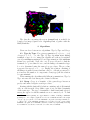
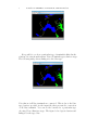
To illustrate the usage of MulTyLink we will use an image clip of
the IP data deemed by Alagador et al., 20111 , consisting of 100 × 100
cells (Figure below).
1Alagador
et al., Linking like with like: optimising connectivity between
environmentally-similar habitats, Landscape Ecology, 27, 291-301, 2012.
MULTYLINK
3
The data file concerning the region (example1.txt) is available for
download at http://purl.oclc.org/multylink, together with the
MulTyLink files.
2. Algorithms
Users can chose between two algorithms: Type by Type and Grasp.
2.1. Type by Type. For a given permutation P = (t1 , t2 , . . . , tm )
of types k = 1, 2, . . . , m, the Type by Type algorithm starts linking
terminals of type k = t1 , using (an adaptation for the node-weighted
case of) a minimum spanning tree based approximation of the minimum
Steiner tree problem2. Next, the cost of every cell used to link the
terminals k = t1 is redefined to zero, and the linkage of terminals of type
k = t2 is determined using the same above procedure. The procedure
is repeated for types k = t3 , . . . , tm . Finally, the solution consisting of
all linkages is pruned from redundant cells (i.e., cells whose removal do
not increase the number of components of any type) till the solution
becomes minimal.
When running the algorithm with different permutations, Type by
Type outcomes the best among the obtained solutions.
2.2. Grasp. Grasp is a heuristic of the general type known as
greedy randomized adaptive search procedure.
Starting with the (unfeasible) solution consisting only of all terminal
cells, at each iteration Grasp links a pair of not yet linked terminals
of the same type. The type of terminals to link is uniformly selected
among the types for which terminals are not connected yet. To link
2The
minimum spanning tree approximation consists of finding a minimum
spanning tree on a complete graph whose nodes are terminals and where the weight
of every edge (u, v) is the cost of the minimum cost path connecting terminal u to
v. Every edge of the minimum spanning tree is replaced by the corresponding
minimum cost path, and a minimal solution is obtained by sequentially removing
non-terminal nodes, whenever removal do not disconnect terminals.
4
R BRÁS, JO CERDEIRA, D ALAGADOR, AND MB ARAÚJO
terminals of the chosen type k, a terminal sk is uniformly selected
from Tk and the path of minimum cost among the minimum cost paths
(excluding barriers) between sk and every other terminal of Tk , not
yet linked with sk , is determined. The path is added to the current
solution, and the costs of its cells are redefined to zero. When all
terminals of the same type are linked (or when no more linkages are
possible), redundant cells (i.e., cells whose removal do not increase
the number of components of any type) are removed till the solution
becomes minimal.
Grasp outcomes the best solution among the solutions obtained
from an arbitrary predefined number of runs.
3. Program interface
Start the program and the main window will appear. Use File→Open
to read your data (see Section 4 for the format of the input file).
While reading the file the log window displays information about
the data read. After reading the data the map window will appear.
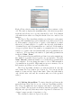
3.1. Selecting parameters. Before solving the problem you may
want to change some parameters. Go to Params→Set Params and open
the window.
MULTYLINK
5
Each cell has a friction value that quantifies the flow resistance of the
cell. The window displays the maximum value of the frictions specified
in the file and allows you to specify a threshold to used. Non terminal
cells with friction values exceeding the threshold are not considered for
linkages.
The Type by Type algorithm calculates one solution for each permutation of the terminals types, and returns the best solution (see Section
2). If the number of types is less or equal to 4, the number of permutations is by default settled to be equal to the factorial of the number
of terminal types, and all permutations are considered. If the number
of types is greater than 4, the number of permutations is by default
settled to be equal to 100, and 100 uniformly selected permutations are
considered. You can change the number of (uniformly) permutations
in the field Num. Perm.
The program solves in parallel the problem for several permutations.
The number of parallel solvers depends on your hardware. The field
Num. threads contains the number of cores that the program finds in
your computer. You can change the value to solve a different number
of permutations in parallel. High numbers use more memory. If you
have memory problems you can lower this value.
The Grasp algorithm calculates one random solution in each run,
and returns the best solution (see Section 2). You can specify the
number of runs and the elapsed time limit. (Since the time limit is
only checked after each run, the execution may exceed the specified
value.)
3.2. Solving the problem. To start solving the problem use the
menu Problem→Solve and choose one of the two algorithms available.
The Grasp algorithm uses more memory and may be inadequate for
large problems. The progress bar will show what the program is doing.
Map size and adjacency rules may render long time for solutions to be
obtained. maps can take a long time to solve.
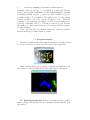
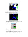
The calculated solution is depicted in yellow.
6
R BRÁS, JO CERDEIRA, D ALAGADOR, AND MB ARAÚJO
It is possible to see how a particular type of terminals is linked in the
solution, choosing from the menu: View→Terminal types solution→type.
The following image shows linkages for the blue type.
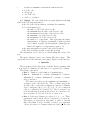
Note that not all blue terminals are connected. This is due to the blue
type barriers specified in the input file that prevent the connection
of all blue terminals. You can see the barriers for a particular type
choosing View→Barriers→type. The figure below depicts barriers and
linkages for the type blue.
MULTYLINK
7
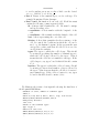
The linkages for type green is shown in the next picture. In this case
the path crosses terminals of type blue. Paths inside terminals are only
shown if these terminals are not selected for display.
3.3. Colour selection. The program has a default set of colours
but you can use your own. To change the colours go to View− >Colours
and change them.
To save your colour scheme go to File− >Save colour scheme and
choose a file name. You can load it any time you want for the same
problem or other problems.
3.4. Cell information. To obtain information about any cell in
the map just click over it. A popup window will appear with:
8
R BRÁS, JO CERDEIRA, D ALAGADOR, AND MB ARAÚJO
•
•
•
•
id of the cell,
cell type(s).
cost of the cell,
x and y coordinates.
3.5.
window
•
•
Output. For each solution the program displays in the log
the following information:
the ids of the cells in solution, excluding the terminals;
for each terminal type:
– the sum of costs of the selected cells,
– the minimum friction value of the selected cells,
– the maximum friction value of the selected cells,
– the minimum cost of the selected cells,
– the maximum cost of the selected cells,
– the number of components. This represents the (minimum) number of clusters of terminals of that type that
can be linked together. (If all terminals of that type are
linked, the number of components is equal to 1.)
• the same information is given for the global solution;
• the wall clock time spent in solving the problem.
The information can be saved to a text file using File→Save solution.
The image displayed can be saved using File→Save image. This
option will create a file with the exact image displayed in the window.
4. Input file
The program reads the data from a text file. Lines beginning with
a # are ignored. Numbers in a line have to be separated by commas.
The format of the file is:
• line 1: Number of cells, number of terminal types.
• line 2: Minimum X coordinate, Maximum X coordinate,
Minimum Y coordinate, Maximum Y coordinate, coordinate
step, zoom factor.
The first four values are the minimum and maximum coordinates of the cells in the file. The coordinate step is the
absolute value of the sum of differences between coordinates
of two contiguous cells, i.e |X − X ′ | + |Y − Y ′ |, for contiguous
cells of coordinates (X, Y ) and (Y, Y ′ ). The zoom factor controls how the map is shown in the screen. A zoom factor of 1
uses one pixel for each cell. A factor of 2 uses 4, etc.
• line 3: Adjacency distances for types k = 1, . . . , m. These
parameters control which cells are considered to be adjacent.
The distance is expressed in step units. A value of d means
that cells within a circle of radius d centred on √a particular
cell are adjacent to it. Common values are 1 and 2. In order
MULTYLINK
9
to avoid rounding errors use a value
a little over the desired
√
one, e.g. 1.001 for 1 or 1.42 for 2.
• line 4: Names of the terminal types, one for each type. For
example Mountains, Plains, Swamps.
• lines 5-end: Information about each cell. Each line must
contain the following comma separated fields:
id: A integer that identifies the cell. Ids must be unique
and in ascending order.
x coordinate: A float number with the longitude of the
cell.
y coordinate: A float number with the latitude of the cell.
cost: A float representing the cost of the cell.
friction: A float that quantifies the flow resistance of the
cell. It controls the conditions in which the cell can be
used, e.g. the human footprint. In the program the user
can specify a value such that all cells above it are discarded from the analysis.
types: The types to which the cell belongs. This should
be an integer specifying the number of terminal types to
which the cell belongs, followed by the types. Value 0
means that the cell is not a terminal for any type. If the
cell belongs to, say, types 5 and 6 this field should contain
2,5,6.
barriers: The types for which the cell is a barrier. Should
be an integer between 0 and number of types, followed by
the types. Value 0 means that the cell is not a barrier to
any terminal type. If the cell is a barrier for, say, types
1,2 and 6 this field should contain 3,1,2,6.
We illustrate the format of an input file showing the first lines of
the file parcial-100-100.txt:
# Number of cells, number of terminal types
23400,2
# Min X coord, Max X, Min Y, Max Y, step, zoom factor
460500,639500,4612500,4741500,1000,6
# Adjacency distance
1.42,1.42
# Name of the terminal types
Type 1,Type 2
# Data for each cell
49409,460500,4741500,0,23,0,2,1,2
49410,461500,4741500,0,20,0,2,1,2
...
10
R BRÁS, JO CERDEIRA, D ALAGADOR, AND MB ARAÚJO
Disclaimer
The authors accept no responsibility for any inconvenience caused
directly or indirectly by the installation or use of this software.
R Brás, Centre for Applied Mathematics and Economics (CEMAPRE),
Instituto Superior de Economia e Gestão, Technical University of
Lisbon, Rua do Quelhas 6, 1200-781 Lisbon, Portugal.
JO Cerdeira, Department of Mathematics, Faculty of Sciences and
Technology, New University of Lisbon, Campus de Caparica, 2829516 Caparica,Portugal and Forest Research Centre (CEF), Instituto
Superior de Agronomia, Technical University of Lisbon (TULisbon),
Tapada da Ajuda, 1349-017 Lisbon, Portugal.
D Alagador, Rui Nabeiro Biodiversity Chair, CIBIO, University
of Évora, Casa Cordovil 2◦ Andar, Rua Dr. Joaquim Henrique da
Fonseca , 7000-890 Évora, Portugal.
MB Araújo, Department of Biodiversity and Evolutionary Biology, Museo Nacional de Ciencias Naturales, CSIC, C/ José Gutiérrez
Abascal, 2, 28006, Madrid, Spain. Rui Nabeiro Biodiversity Chair,
CIBIO, University of Évora, Casa Cordovil 2◦ Andar, Rua Dr. Joaquim
Henrique da Fonseca , 7000-890 Évora, Portugal.