Download Introducing hierarchy, abstraction, namespaces and relays

TECHNISCHE UNIVERSITEIT EINDHOVEN
Department of Mathematics and Computer Science
The ToolBus: Introducing
hierarchy, abstraction,
namespaces and relays
By
Dennis Hendriks
Supervisors:
Mark van den Brand (TU/e)
Merijn de Jonge (Philips Research)
Eindhoven, October 27, 2007
Abstract
Software systems become larger, more complex and often consist of distributed,
heterogeneous parts. A coordination architecture can be used to facilitate the
communication between the parts, to control the coordination, to abstract away
low level details and to allow for structuring of the system. In this thesis the
focus is on the abstraction mechanisms and layered structures of coordination
architectures. In particular, it discusses the design and implementation of hierarchical abstraction mechanisms in the ToolBus coordination architecture,
which can be seen as a first step towards dependable ToolBus systems. Specifically, a hierarchical process structure is introduced along with a communication
restriction that enforces abstraction. This restriction has some disadvantages,
mainly in the form of chaining, which will be solved by introducing relays. Furthermore, namespaces are introduced as a solution to name clashes of messages
and they provide additional (optional) abstraction as well. Finally, a validation
is performed on some examples and the implementation details as well as future
work are discussed.
Acknowledgements
I would like to thank all of you who helped, guided and supported me throughout
my master’s project, as well as all of you who expressed an interest in my project.
In particular, I would like to thank my supervisor Prof. Dr. Mark van den Brand
for introducing me to the ToolBus project, for guiding me and for providing
valuable feedback throughout the project.
I would also like to thank my other supervisor Dr. Merijn de Jonge, Senior
Scientist at Philips Research Laboratories, for initiating the idea for this project
as well as for his guidance and feedback throughout the project.
Then I would like to thank Prof. Dr. Paul Klint of the Center for Mathematics
and Computer Science (CWI) for the fruitful discussions that we had on among
others the direction of the project and the ToolBus in general, as well as for his
pragmatic and realistic views and to the point suggestions.
Furthermore, I would like to thank all the other people of the CWI who attended
my PEM presentation or contributed in any other way, in particular Dr. Jurgen
Vinju and Arnold Lankamp.
Finally, I would like to thank the TU/e for providing me with the opportunity
to do this master’s project, all the people of the Eindhoven University of Technology (TU/e) that contributed in any way to my project and my family and
friends who supported me throughout the project.
i
Contents
1 Introduction
1
2 Coordination architectures
2.1 Properties . . . . . . . . . . . . . . . . . . . . . . . . . . . . . . .
2.2 Differences . . . . . . . . . . . . . . . . . . . . . . . . . . . . . . .
3
3
5
3 The ToolBus coordination architecture
3.1 Compiler system example . . . . . . . . . . . . . . . . . . . . . .
7
12
4 Related literature
4.1 Manifold . . . . . .
4.2 Sophtalk . . . . . .
4.3 Field . . . . . . . .
4.4 CORBA . . . . . .
4.5 Service Component
4.6 Koala . . . . . . .
4.7 Overview . . . . .
14
14
15
16
18
19
21
22
. . . . . . . . . . . .
. . . . . . . . . . . .
. . . . . . . . . . . .
. . . . . . . . . . . .
Architecture (SCA)
. . . . . . . . . . . .
. . . . . . . . . . . .
.
.
.
.
.
.
.
.
.
.
.
.
.
.
.
.
.
.
.
.
.
.
.
.
.
.
.
.
.
.
.
.
.
.
.
.
.
.
.
.
.
.
.
.
.
.
.
.
.
.
.
.
.
.
.
.
.
.
.
.
.
.
.
.
.
.
.
.
.
.
.
.
.
.
.
.
.
.
.
.
.
.
.
.
.
.
.
.
.
.
.
.
.
.
.
.
.
.
5 Problem introduction
25
5.1 The need for additional structure . . . . . . . . . . . . . . . . . . 25
5.2 Introducing Structured Process Groups . . . . . . . . . . . . . . 28
6 The solution: hierarchy, abstraction, namespaces and relays
6.1 Hierarchical processes . . . . . . . . . . . . . . . . . . . . . . .
6.1.1 The current situation . . . . . . . . . . . . . . . . . . .
6.1.2 Introducing hierarchical processes . . . . . . . . . . . .
6.1.3 Note on toolbus(...) construct . . . . . . . . . . . . .
6.1.4 Dealing with cycles . . . . . . . . . . . . . . . . . . . . .
6.1.5 Top level process . . . . . . . . . . . . . . . . . . . . . .
6.2 Hierarchical processes and communication . . . . . . . . . . . .
6.2.1 Current situation . . . . . . . . . . . . . . . . . . . . . .
6.2.2 Abstraction . . . . . . . . . . . . . . . . . . . . . . . . .
6.2.3 Chaining . . . . . . . . . . . . . . . . . . . . . . . . . .
6.2.4 Relays . . . . . . . . . . . . . . . . . . . . . . . . . . . .
6.2.5 Summary . . . . . . . . . . . . . . . . . . . . . . . . . .
6.3 Namespaces . . . . . . . . . . . . . . . . . . . . . . . . . . . . .
6.3.1 An example . . . . . . . . . . . . . . . . . . . . . . . . .
6.3.2 Instantiating processes in namespaces . . . . . . . . . .
6.3.3 Absolute vs. relative namespaces . . . . . . . . . . . . .
6.3.4 Communication actions and namespaces . . . . . . . . .
6.3.5 Some additional examples . . . . . . . . . . . . . . . . .
6.4 Chaining and relays revisited . . . . . . . . . . . . . . . . . . .
6.4.1 Relays with namespaces . . . . . . . . . . . . . . . . . .
6.4.2 Connects relays . . . . . . . . . . . . . . . . . . . . . . .
6.4.3 Another example of relays . . . . . . . . . . . . . . . . .
6.4.4 Direction of relays . . . . . . . . . . . . . . . . . . . . .
6.4.5 Note on relay targets . . . . . . . . . . . . . . . . . . . .
6.5 Summary . . . . . . . . . . . . . . . . . . . . . . . . . . . . . .
ii
.
.
.
.
.
.
.
.
.
.
.
.
.
.
.
.
.
.
.
.
.
.
.
.
.
30
30
30
31
32
32
33
34
34
34
35
37
38
39
39
39
41
42
43
45
45
46
48
48
49
49
6.6
6.7
6.8
6.9
Example of direct communication
Syntax considerations . . . . . .
Orthogonality of solutions . . . .
Summary . . . . . . . . . . . . .
.
.
.
.
.
.
.
.
.
.
.
.
.
.
.
.
.
.
.
.
.
.
.
.
.
.
.
.
.
.
.
.
.
.
.
.
.
.
.
.
.
.
.
.
.
.
.
.
.
.
.
.
.
.
.
.
.
.
.
.
.
.
.
.
.
.
.
.
.
.
.
.
50
51
51
52
7 Requirements revisited
7.1 Hierarchy (R1) and Abstraction (R2) . . . . .
7.2 Interfaces (R3) . . . . . . . . . . . . . . . . .
7.2.1 Definition and examples . . . . . . . .
7.2.2 Internal vs. external communication .
7.2.3 Benefit of interfaces . . . . . . . . . .
7.2.4 Summary . . . . . . . . . . . . . . . .
7.3 Evolution and reuse (R4) . . . . . . . . . . .
7.4 Semantics (R5) and formal foundation (R7) .
7.5 Backwards compatibility (R6) . . . . . . . . .
7.6 Performance (R8) . . . . . . . . . . . . . . . .
7.7 Name clashes (R9) . . . . . . . . . . . . . . .
7.8 Dependability (R10) . . . . . . . . . . . . . .
7.8.1 Example 1 . . . . . . . . . . . . . . . .
7.8.2 Example 2 . . . . . . . . . . . . . . . .
7.9 Analysis of matching communication actions
7.9.1 Dynamic checking . . . . . . . . . . .
7.9.2 Static checking . . . . . . . . . . . . .
.
.
.
.
.
.
.
.
.
.
.
.
.
.
.
.
.
.
.
.
.
.
.
.
.
.
.
.
.
.
.
.
.
.
.
.
.
.
.
.
.
.
.
.
.
.
.
.
.
.
.
.
.
.
.
.
.
.
.
.
.
.
.
.
.
.
.
.
.
.
.
.
.
.
.
.
.
.
.
.
.
.
.
.
.
.
.
.
.
.
.
.
.
.
.
.
.
.
.
.
.
.
.
.
.
.
.
.
.
.
.
.
.
.
.
.
.
.
.
.
.
.
.
.
.
.
.
.
.
.
.
.
.
.
.
.
.
.
.
.
.
.
.
.
.
.
.
.
.
.
.
.
.
.
.
.
.
.
.
.
.
.
.
.
.
.
.
.
.
.
.
.
.
.
.
.
.
.
.
.
.
.
.
.
.
.
.
53
53
53
53
54
55
56
56
56
57
57
58
58
58
58
59
59
59
8 Validation
61
8.1 The MouseClicked scenario . . . . . . . . . . . . . . . . . . . . . 61
8.2 The compiler system example revisited . . . . . . . . . . . . . . . 63
9 Implementation
9.1 Translation . . . . . . . . . . . . .
9.2 Native support . . . . . . . . . . .
9.2.1 Benefit . . . . . . . . . . . .
9.2.2 The ToolBusNG explained .
9.2.3 Implementation details . . .
.
.
.
.
.
.
.
.
.
.
.
.
.
.
.
.
.
.
.
.
.
.
.
.
.
.
.
.
.
.
.
.
.
.
.
.
.
.
.
.
.
.
.
.
.
.
.
.
.
.
.
.
.
.
.
.
.
.
.
.
.
.
.
.
.
.
.
.
.
.
.
.
.
.
.
.
.
.
.
.
.
.
.
.
.
66
66
66
66
66
67
10 Conclusions
69
10.1 Requirements . . . . . . . . . . . . . . . . . . . . . . . . . . . . . 69
10.2 Usefulness in practice . . . . . . . . . . . . . . . . . . . . . . . . 70
10.3 Final conclusion . . . . . . . . . . . . . . . . . . . . . . . . . . . 70
11 Future work
11.1 Real life testing . . . . . . . . . . . .
11.2 Compatibility . . . . . . . . . . . . .
11.3 Dynamic namespaces . . . . . . . . .
11.4 Process namespaces . . . . . . . . .
11.5 Protocols . . . . . . . . . . . . . . .
11.6 Cycle detection . . . . . . . . . . . .
11.7 Interfaces . . . . . . . . . . . . . . .
11.8 Analysis of matching communication
11.9 Semantics and formal foundation . .
iii
. . . . .
. . . . .
. . . . .
. . . . .
. . . . .
. . . . .
. . . . .
actions
. . . . .
.
.
.
.
.
.
.
.
.
.
.
.
.
.
.
.
.
.
.
.
.
.
.
.
.
.
.
.
.
.
.
.
.
.
.
.
.
.
.
.
.
.
.
.
.
.
.
.
.
.
.
.
.
.
.
.
.
.
.
.
.
.
.
.
.
.
.
.
.
.
.
.
.
.
.
.
.
.
.
.
.
.
.
.
.
.
.
.
.
.
.
.
.
.
.
.
.
.
.
71
71
71
71
72
72
72
72
73
73
11.10Dependability . . . . . . . . . . . . . . . . . . . . . . . . . . . . .
A SDF syntax of T scripts
B T script translation
B.1 Example . . . . . . . . .
B.2 The top of the hierarchy
B.3 Process names . . . . .
B.4 Communications . . . .
74
76
.
.
.
.
.
.
.
.
.
.
.
.
.
.
.
.
iv
.
.
.
.
.
.
.
.
.
.
.
.
.
.
.
.
.
.
.
.
.
.
.
.
.
.
.
.
.
.
.
.
.
.
.
.
.
.
.
.
.
.
.
.
.
.
.
.
.
.
.
.
.
.
.
.
.
.
.
.
.
.
.
.
.
.
.
.
.
.
.
.
.
.
.
.
81
81
81
81
82
1
Introduction
In the development of large software systems, there is often much competition
from companies that develop similar software. Due to this competition, new
software must be developed in a short amount of time, making it impossible
to create it entirely from scratch. The well-known solution to this problem is
to reuse existing software parts [18] (often called components). Also, existing
legacy software systems become more and more complex over time [22], mainly
because new features are constantly added. Often ad-hoc solutions are used to
add the new features, without regard for the architecture of the entire system,
which makes such systems harder and harder to maintain. It is good practice
to decompose such systems into parts that have clearly defined and coherent
functionality [34]. So, both in the development of new software systems as well
as in the decomposition of legacy systems, we end up with a system consisting
of components.
Individual parts of a system do not generally run in complete isolation; communication between the parts is needed. Therefore, the parts that together form
the system need to be integrated to compose the actual system. This raises the
question of how to perform this integration and how to describe and analyze the
communication between those parts. Today, in many systems, communication
may also span multiple machines within a network. Combined with the fact
that when systems get larger, the communication usually increases, it makes
those questions even harder to answer.
This master’s thesis is concerned with coordination architectures or coordination frameworks, which allow for the coordination of separate activities within
a system. They form a solution to the problem described earlier: the integration of and communication between software components. In particular we are
interested in the abstraction mechanisms and layered structures of coordination
architectures. The largest part of this thesis will be about the design and implementation of hierarchical abstraction mechanisms in a coordination architecture
called the ToolBus.
Philips is a company that among other things builds consumer electronics and
medical systems, which contain embedded software. They use third party software components and are therefore confronted with the problem of integrating
the components with the other software in their systems. Dependability has
always been an important issue in the design of embedded software systems.
Recently, Philips is focusing some of its research on fault tolerance and selfhealing (both in hardware [29] and software [35, 16]), that can be used to increase dependability, especially when integrating third party software. Philips
is interested to see if systems running in the ToolBus can be made dependable
and this project is a first step in that direction.
The outline of this thesis is as follows. In Section 2 coordination architectures
will be introduced and their properties will be discussed. Then one particular
coordination architecture, called the ToolBus, will be introduced in Section 3.
This is followed by a discussion of literature on coordination architectures (Section 4). Section 5 discusses some of the problems related to the ToolBus (most
1
notably the lack of structure) as well as the requirements on a solution to the
structure-related problems. In Section 6 the proposed solution will be described
in detail, including the motivation for choosing this particular solution. This is
followed by Section 7, which discusses the relation between the solution and the
requirements. Then, in Section 8, a validation of the solution will be performed
by investigating the benefit of the changes to some examples. Section 9 deals
with all implementation aspects and in Section 10 the conclusions of the entire
project are drawn. Finally, Section 11 contains some possibilities for future
research.
2
2
Coordination architectures
The previous section introduced coordination architectures as a solution to the
problem of integrating software components and describing and analyzing the
communication between them. In this section, a more extended introduction to
coordination architectures (and their properties) will be given.
Well-structured systems usually consist of several (cohesive) parts. In the early
days of software systems, parts were just subroutines in programming languages.
Later on, parallel systems allowed for the parallel execution of parts (usually
called tasks). With the introduction of object models and class hierarchies the
focus of parts shifted from subroutines to classes and (cohesive) collections of
classes. Nowadays, parts are generally referred to as components. However, the
term component is used both to refer to a collection of classes as well as to
refer to a part of a system in general. Even more recent as components is the
notion of open systems [23], in which parts of the system (called agents) may
dynamically join (and later leave) the system.
Coordination architectures go beyond anything that existed previously; they go
beyond parallel systems, beyond object models and class hierarchies and beyond
open systems. There are a lot of definitions of what exactly a coordination
architecture is. Some of these definitions include “the glue that binds separate
activities into an ensemble” [17], “a means of integrating a number of possibly
heterogeneous components together, by interfacing with each component in such
a way that the collective set forms a single application that can execute on and
take advantage of parallel and distributed systems” [32], “meant to close the
conceptual gap between the cooperation model of an application and the lowerlevel communication model used in its implementation” [3] and “provides a
framework in which the interaction of active and independent entities called
agents can be expressed” [13].
The common factor is that coordination architectures can be used to coordinate
the interactions between the different parts of an application, thereby supporting (or facilitating) the (high-level) integration of software systems. However,
the way in which the coordination of the communication between the parts
of a system is achieved, is one of the biggest differences between the existing
coordination architectures.
The impact of coordination architectures on software development is significant,
as “coordination is relevant in design, development, debugging, maintenance,
and reuse of all concurrent systems” [3]. Also, the issues in coordination are
not just computer science related; coordination is an interdisciplinary issue and
includes issues from “organization theory, economics, and biology” [30].
2.1
Properties
Since there are a lot of different definitions of coordination architectures, it
is extremely difficult (if not impossible) to give a list of properties that all
coordination architectures must satisfy. It is however possible to give a list of
3
properties that are often associated with coordination architectures and that
are satisfied by a lot of them. What follows is a discussion of these properties
(or features), including why they are important:
Integration Providing a means to integrate the different parts of a system,
by facilitating the communication between those parts. This is the essence
of a coordination architecture. However, the way that the integration is
achieved is one of the biggest differences between the existing coordination architectures. Also, when the parts of the system are integrated,
there is still a difference in how the coordination architecture determines
which parts will communicate and which restrictions are imposed on that
communication.
Abstraction of computation Enforcing a strict separation of computation
(in the different parts of the system) and communication (at a higher
level), allowing for the computation parts to be abstracted away. This
should decrease the number of dependencies between the different parts
of the system (decreased coupling). Also, the computation parts of the
system are often not aware of whom they communicate with or how the
system is composed. The communication parts connect to the system via
some interface and that is all they need to know. This is one the most
important properties of coordination architectures.
Heterogeneity Allowing the integration of software components written in
different programming languages and running on any computer platform.
This allows for legacy systems to be integrated into a system together
with newer systems. Also, it allows one to write parts of the system in the
language that is best suited for that particular part and it makes systems
highly portable. The downside is that conversions are usually needed
to make sure the components written in different languages can actually
communicate and cooperate, giving rise to decreased performance.
Distributivity Allowing the integration of software components running
on different physical machines, for example within a Local Area Network
(LAN). This way, the application can be distributed over several machines,
thereby increasing the available resources, such as processing power and
memory. However, in order for components running on different machines
to communicate, network communication is needed. Compared to components running on a single machine, this results in a performance penalty,
which may be considerable!
Abstraction of communication Hiding the (low-level) details of the communication, such that programmers need not be concerned with them. The
different parts of the system simply interface with the coordination system.
They don’t have to concern themselves with details of the communication,
like where the receiver is located and what communication protocols or
media are used. All coordination architectures hide some communication
details, but there are differences. Using more ‘higher level’ communication concepts gives you less control over the details of the communication,
thereby possibly decreasing the performance.
4
Structure/Hierarchy/Abstraction of composition Stimulating the introduction of structure in the system, by grouping parts of the system together
into what we will call components or subsystems. It is then possible to
structure the system even further, by introducing a hierarchy (on components) into the system architecture. Finally we can hide the internal
details of the components, to obtain an abstraction on the composition of
the system (internal details are encapsulated). Introducing structure has
several advantages, which include easier maintenance, improved scalability, decreased coupling and stimulation of reuse.
Dynamic Architecture Providing the means for the architecture to change
during execution, allowing parts to be added to or removed from the system (at runtime). This way maintenance can be performed on the system
while it is running; it is not necessary for the system to go off-line to update it. The downside is that extra administration is needed, as well as
mechanisms to facilitate the dynamic restructuring. These mechanisms
require resources as well.
Supporting distributivity has clear advantages, but there is a performance penalty. This is true for many features of coordination architectures. It depends
on the requirements for a coordination architecture, whether or not it should
support certain features. The key here is to balance a rich feature set with issues
like performance.
2.2
Differences
We have now seen the properties that (most) coordination architectures satisfy.
Existing coordination architectures differ from one another by the amount of
properties they satisfy, the extent to which they satisfy them and by how they
are satisfied. However, besides those properties, there are several other areas in
which they can differ:
Formal foundation Some coordination architectures have a formal foundation, including formal semantics. This allows for formal reasoning and
analysis of the communication.
Data- vs. control-driven Some coordination architectures are data-driven
and others are control-driven [32]. Data-driven coordination architectures
evolve around what happens to the data. They usually have some sort of
database that contains a large collection of data, which is shared among
the parts of the system. Control-driven coordination architectures evolve
around the flow of control.
Endogenous vs. Exogenous Closely related to ‘data- vs. control-driven’
is endogenous vs. exogenous coordination [32]. Endogenous coordination
is coordination from ‘within’; coordination is mixed in the computation.
Exogenous coordination is coordination from ‘without’; coordination is
not contained inside the module itself.
5
Application domain Some coordination architectures are designed for a
specific application domain, while others are more general and can be
used in many application domains.
Implementation status Some coordination architectures are not yet implemented, while some have existed for years and are widely used in practice.
Others are no longer under development.
(A)synchronous communication There are coordination architectures that
only support synchronous communication, those that only support asynchronous communication and those that support both. Also, some systems support point-to-point connections; some only support (selective)
broadcasting. Other systems even support both. Combining these two
characteristics results in four different forms of communication: synchronous point-to-point, asynchronous point-to-point, synchronous (selective)
broadcast and asynchronous (selective) broadcast.
Data format used Data plays a role in every coordination architecture; it
may be more important in data-driven architectures than it is in controldriven ones, but it always plays a role. Data must be represented in
some form. Different coordination architectures use different formats to
represent data.
Execution Some coordination architectures require compilation of source
files before execution, while others interpret source scripts at runtime. Applications that communicate via the coordination architecture may need
extra code to be compiled with it to be able to communicate with the
rest of the system. Also, conversions between the data formats used by
the application and the data formats used in the coordination architecture
may be needed.
Language used The languages that coordination architectures use to describe the communications within a system differ. Some use existing languages, while others invent new ones.
Some of the details of the differences that are described above may not be completely clear, but that is not a problem. The goal of the above discussion is
to very shortly introduce some of the differences between coordination architectures. These differences will play an important role in the next sections, in
particular Section 4.
6
3
The ToolBus coordination architecture
The ToolBus [8, 9, 26, 10, 25, 14] coordination architecture is being developed
at the University of Amsterdam and the CWI (the Dutch National Research
Institute for Mathematics and Computer Science). The name ‘ToolBus’ comes
from the link to hardware busses. The ToolBus can be seen as the software
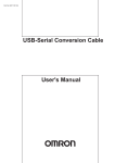
equivalent: a software bus. Applications (which are called tools) that are connected to this bus are part of the system. Figure 1 gives an overview of an
example ToolBus system. Note however that it is an abstract example that just
shows all the important concepts.
Figure 1: An example ToolBus system
It is important to note that within the ToolBus architecture, computation and
coordination are completely separated, since the ToolBus itself does (in principle) not perform any computations, but only coordinates the communication.
It can therefore be said that the ToolBus is control-driven and exogenous. The
computations are done by the tools (the external applications). Tools are not
allowed to communicate with each other directly, but only via the ToolBus.
This is also visible in Figure 1. Since tools interface with the ToolBus via a
strict interface, the ToolBus does not concern itself with the internals of the
tools or the computations they perform. Thus, strict separation of computation
and coordination effectively abstracts away from the computation part of the
system.
The ToolBus is programmed with so called ToolBus scripts. These ToolBus
scripts, or T scripts for short, are based on ACP (Algebra of Communicating
Processes [4]). The T scripts contain process descriptions that describe all possible communication behavior of the tools. There may be one process for each
tool, but there are no restrictions here; there may be extra processes and a
single process may communicate with more than one tool. In Figure 1, the
ellipses denote processes. Note that for Tool 1, there is only a single process
that controls all communication with that tool. If the only goal of a process
7
is to interface between the tool and the rest of the system, it is called an idef
(Interface Definition), as it defines the interface (behavior) of that tool. Tool 2
however, receives messages from both processes P3 and P5. The use of an idef
for each tool is currently common practice. T scripts support most of the process
algebra operations. Beside atomic actions, these include sequential composition
(.), choice (+), iteration (*), the delta action (delta) and parallel composition
(k). Some extensions are included as well, like the introduction of (local) variables (let ... in ... endlet) and assignments and expressions on variables
(V := E). See Table 11 for a more complete overview of the primitives that
can be used in T scripts. The behavior of the whole system is defined as the
parallel composition of all processes in the initial configuration (toolbus(...)
keywords).
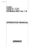
Figure 2 shows an example T script for the system of Figure 1 (except for the
definition of processes P1, P2, P4 and P5, which are omitted). In the first line,
the definitions from the file tool1.idef are included. After that, process P3
is defined. Three local variables are declared (variable T is of type tool2; variables I and J are of type int). The actual definition of the behavior of the
process starts after the in keyword. First the process subscribes to a note, then
it executes a tool. The rest is an iteration that consists of a choice. The first
alternative is to receive a message, send a request to the tool, receive an answer
from the tool and then send a message. The second alternative is to receive a
note and then send a message. Since the iteration ends with a delta primitive
that can never be chosen, the iteration iterates indefinitely. Almost at the end
we see the definition of tool2 with the command that needs to be executed
to get the tool running. Finally, we see that processes P1, P2, P3, P4 and P5
should initially be created.
#include <tool1.idef>
process P3 is
let T : tool2,
I : int,
J : int
in subscribe(somenote(<int>, <int>)) .
execute(tool2, T?) .
( ( rec-msg(some-msg(I?)) .
snd-eval(T, some-tool-message(I)) .
rec-value(T, some-tool-answer(I?)) .
snd-msg(some-other-msg(I))
) + (
rec-note(somenote(I?, J?)) .
snd-msg(some-other-msg(J))
)
) * delta
endlet
tool tool2 is {command = "./tool2"}
toolbus(P1, P2, P3, P4, P5)
Figure 2: An example T script
Unlike most other coordination architectures, the ToolBus has a solid formal
foundation, since processes are defined in a process algebra syntax. Also, the
ToolBus describes all the interactions between the tools, providing complete
1 This
table is based on Appendix E from [25].
8
Primitive
process ... is ...
tool ... is ...
toolbus(...)
let ... in ... endlet
create(...)
delta
P1 + P2
P1 . P2
P1 * P2
P1 k P2
snd-msg(...)
rec-msg(...)
snd-note(...)
rec-note(...)
no-note(...)
subscribe(...)
unsubscribe(...)
snd-eval(...)
rec-value(...)
snd-do(...)
rec-event(...)
snd-ack-event(...)
rec-connect(...)
rec-disconnect(...)
execute(...)
snd-terminate(...)
shutdown(...)
if ... then ... fi
if ... then ... else ... fi
V := E
delay(...)
abs-delay(...)
timeout(...)
abs-timeout(...)
printf(...)
Description
process definition
tool definition
ToolBus configuration (initial process
creation)
local variables
(dynamic) process creation
inaction (deadlock)
alternative composition (choice between
alternatives P1 and P2 )
sequential composition (P1 followed by
P2 )
iteration (zero or more times P1 followed by P2 )
parallel composition (communication
free merge)
send a message (binary, synchronous)
receive a message (binary, synchronous)
send a note (broadcast, asynchronous)
receive a note (asynchronous)
no notes available for process
subscribe to notes
unsubscribe from notes
send evaluation request to tool
receive a value from a tool
send request to tool (no return value)
receive event from tool
acknowledge a previous event from a
tool
receive a connection request from a tool
receive a disconnection request from a
tool
execute a tool
terminate the execution of a tool
terminate the ToolBus
guarded command
conditional expression
assignment
relative time delay
absolute time delay
relative timeout
absolute timeout
print formatted ToolBus terms to console
Table 1: Overview of ToolBus primitives
9
control over the tool communications. The behavior of the system is based on
the semantics of process algebra, which makes it possible to formally reason
about the communication within the ToolBus. By analyzing ToolBus communication, properties of the system can be proved formally.
Process definitions may include actions for starting and terminating tools (like
execute(...) in Figure 2). The operating system commands that must be
executed to start a tool are also defined in the T scripts. Another possibility is
to connect to (or disconnect from) tools that are started independently of the
ToolBus.
There are two methods of communication between processes inside the ToolBus:
messages and notes. When using messages, one process (using the snd-msg
action) sends a message and another process2 (using the rec-msg action) receives
the message. This communication is synchronous. To receive notes, a process
must first subscribe to it. Then, when a process sends a note (using the snd-note
action), all processes that are subscribed to that note will receive it (using the
rec-note action). This is a form of asynchronous selective broadcasting. The
dotted arrows in Figure 1 are an example of a note being received by two other
processes.
Communication between processes and tools is different. Processes may send
messages by using the snd-eval, snd-do and snd-ack-event actions, while tools
may use the snd-event and snd-value actions. As mentioned earlier, there is no
direct communication between tools.
All communication via the ToolBus is encoded in ATerms [11, 15]. ATerms are a
language and platform independent way of representing data. Maximal subterm
sharing is supported, which decreases memory use and allows for simple and fast
equality checking. The very concise binary exchange format makes this term
format ideal for communication. Examples of ATerms from Figure 2 include
somenote(I?, J?) and some-other-msg(J).
Tools that communicate via the ToolBus may be written in any programming
language. To interface with the ToolBus, a language-specific adapter is needed.
Such an adapter helps tools to support the message protocols of the ToolBus
and it helps in the use of ATerms. This way the ToolBus can be used, without
programmers having to be concerned too much with the details of the communication. Adapters for several languages, including Perl, Python and Tcl/Tk
are available. Figure 1 shows two tools. Tool 1 uses a generic adapter for the
Perl language. Tool 2 is written in C and uses two libraries (one for the ToolBus
connection and one for ATerms). In the case of Tool 2, the adapter is sort of
integrated in the tool. Tools may also be distributed over several machines with
different hardware platforms. Tools interface with the ToolBus using TCP/IP
sockets, but the details of this are hidden by the adapters. The ToolBus also
hides other details of the communication (like for instance on which machines
the other tools run) from the tools.
ToolBus scripts are static, they don’t change during execution. The ToolBus
2 The ToolBus doesn’t explicitly support sending messages to a specific process. More
information on this follows in the remainder of this section.
10
can be started with only a single script as it parameter, but scripts can include
other scripts. The ToolBus executes scripts by interpreting them.
The ToolBus coordination architecture does not use named ports to connect
parts of the system that may communicate. Instead, pattern matching on
ATerms is performed by the ToolBus to determine which processes and tools
communicate. As a consequence of this, it cannot (conclusively) be determined beforehand which process will receive a certain message. For example, in Figure 1 you see that process P3 sends out ATerms with signature
some-other-msg(<int>). Both processes P4 and P5 can receive such a message
and if both rec-msg actions are enabled at the same time, a non-deterministic
choice will be made (and only one of them actually receives the message!).
It is important to realize that user-defined data types are not present in the
ToolBus, unlike in several other existing coordination architectures. However,
ATerms are an encoding of user-defined data types. Therefore, even though
user-defined data types may not be present in the syntax of T scripts, they are
supported, since ATerms are used. Only a small set of built-in operations on
ATerms is provided, which is sufficient, since only tools should manipulate data
(and not the T scripts).
The ToolBus has been used for the renovation of the ASF+SDF Meta-Environment [24, 37, 38, 36], which was the reason the ToolBus was developed in the
first place. Currently, it is one of the largest projects using the ToolBus system.
It consists of almost 40 tools and about 300 process definitions, which is quite
a lot. However, the ToolBus can also be used to support a multi-user game site
with thousands of users3 . This shows that the ToolBus is not limited to a single
application domain, but can be used for very different types of applications.
Visit http://www.cwi.nl/htbin/sen1/twiki/bin/view/SEN1/ToolBus for the official ToolBus website. Extensive information on the first design of the ToolBus
can be found in [8]. More information on applications that have been implemented by using ToolBus technology can be found in [26]. The second (and
current) version of the ToolBus is the Discrete Time ToolBus, which includes
several extensions, including time primitives. Extensive information on this second design of the ToolBus can be found in [9, 10]. A summary of the experiences
that have been gained in the ToolBus project so far as well as a sketch of some
preliminary ideas on how the ToolBus can be further improved, can be found
in [14]. Information that is useful for ToolBus programmers can be found in [25].
The ToolBus is currently under active development. The first two versions were
implemented in C. A new version is being implemented in Java.
Next, a bigger example system will be introduced. It is added to show what an
actual ToolBus system looks like, to motivate some of the problems with the
current ToolBus (Section 5.1) and to validate the solution to those problems
(Section 8.2).
3 In
the Acknowledgments section of [14], it is stated that www.gamesquare.nl will be made
ToolBus enabled. In Section 6 it is stated that the new Java implementation of the ToolBus
aims at supporting such sites.
11
3.1
Compiler system example
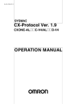
Figure 3: The compiler system example
12
It is now time to introduce a somewhat larger system: a compiler system that
can be used to compile both Java and C++ source code for both Windows
and Linux systems. The compiler system includes a code optimizer, a graphical
user interface (GUI) and an (external) editor. See Figure 3 for an overview
of the architecture of the compiler system (ignore the information related to
‘structured process group with interface’ for now). Note however, that the
ATerm signatures of the messages are incomplete, as only the names of the
messages are included.
There are nine tools, each with its own idef (process). The GUI tool/idef can
signal the Control process that the user has requested an action (load a source
file, save a source file or compile all source files). The Control process connects
all the parts of the system. It will ask the I-O process to perform the saving
and loading of the source files; it will send the loaded source code to the Editor ;
it will request the current code from the Editor before compilation; and it will
ask the Compiler process to compile the code. The Control process can send
messages (about compilation errors etc.) to the GUI, which will then display
them. Also, the Editor can indicate that the source code has changed by sending
a note.
The remaining part of the system is concerned with the actual compilation. The
Compiler process sends the code to either the JavaCompiler or the CPPCompiler, which will create Intermediate Language (IL) code. The CPPCompiler is
implemented by a single tool. The JavaCompiler is implemented by means of
two separate tools, a parser (JavaParser ) and an IL code generator (JavaCodeGen). Both the Java and C++ compiler can send out an il-compile-err message,
or a compile-rslt message. The OptimizeCode process can receive compile-rslt
messages, which include the IL code. The code optimizer will optimize the
code and send it back to the Compiler process, which will then ask the TargetCodeGen process to generate target platform code for Windows (WinCodeGen
process) or Linux (LinuxCodeGen process). The WinCodeGen and LinuxCodeGen processes are instantiated by the TargetCodeGen process.
13
4
Related literature
In this section, some other coordination architectures as well as related languages and systems that have been described in literature are discussed. Special interest will go out to the abstraction and modularization possibilities of
those systems. At the end of this section there is an overview of all described
coordination architectures and their properties.
4.1
Manifold
Manifold [1, 2] is a coordination architecture that was developed at the Center
for Mathematics and Computer Science (CWI) in The Netherlands, just like
the ToolBus. It is an implementation of a generic communication model, which
is referred to as the Idealized Worker Idealized Manager (IWIM) model. This
model enforces a strict separation of computation (by workers) and coordination
(by managers). The ‘idealized’ means that workers process input, do some kind
of computation and produce output, without knowing where the input comes
from, where the output goes (this is also called ‘anonymous communication’)
or how the system is build up (composed). For managers something similar
holds; managers can create worker instances and (dis)connect them, without
being concerned with what computation the workers perform and how they do
it.
In the IWIM model, a process is a black box with well defined ports through
which it can exchange information with its environment. There is a distinction
between input and output ports. An input and an output port can be connected
by a stream. Independent of the communication by streams, there is the notion
of events. Processes need to register to receive certain events. Compositionality
is a key concept of the IWIM model. A manager process that connects several
worker processes together can be seen as a worker process by a higher-level
manager. In this way, a hierarchy is introduced.
The Manifold coordination language can be used to create program modules (coordinator processes) that describe the interconnections (coordination) between
the different processes that make up the application. The language is stronglytyped, block-structured, declarative and event-driven. Since connections can
be dynamically created and destroyed, the architecture of a system constantly
changes at runtime. A module encapsulates all that is declared inside, which
corresponds nicely to the idea of processes being black boxes. So, there is a
strong notion of abstraction.
The Manifold system consists of a library of built-in and predefined functions of
general interest and a number of utilities, like a compiler and a runtime system.
External processes may be written in any programming language and they may
be running on different heterogeneous machines within a network. The Manifold
system will take care of separate compilation and runtime mapping of modules
to nodes.
14
Comparison with the ToolBus
The ToolBus and Manifold share a key goal: the strict separation of computation and communication. Also, both allow heterogeneous tools in a distributed
environment.
However, there are also several striking differences. In the Manifold system,
compositionality and abstraction are key concepts, while they are almost completely absent in the ToolBus. Furthermore, the ToolBus supports both synchronous and asynchronous communication, while Manifold only supports asynchronous communication4 . Manifold programs have to be compiled beforehand,
while ToolBus scripts are interpreted at runtime. Finally, the Manifold modules are described in what can be seen as a (specially designed) programming
language, while ToolBus script have a more formal foundation, since they are
based on process algebra.
4.2
Sophtalk
Sophtalk [20, 21] is a coordination architecture that was developed at the Institute National de Recherche en Informatique et en Automatique (INRIA) in
France. The most important notion in Sophtalk is the stnode (Sophtalk node).
There are two kinds of stnodes; an atomic stnode encapsulates an (external)
tool and a non-atomic stnode encapsulates other (atomic and/or non-atomic)
stnodes. In this way a strict hierarchy is introduced.
Stnodes can have multiple input and output ports, all of which have a name. All
input and output ports with the same name on the same level5 are connected
by a so called bus line. This gives rise to multicast communication; when an
stnode sends out a message on one of its output ports, it will be put on the bus
line. It will then be received by all stnodes that have one of their input ports
connected to that bus line. If the parent stnode has an output port connected
to this bus line, it will propagate the message outward. If there are no stnodes
‘listening’ to the message, it will fall on deaf ears. Ports only have simple names
and no types. This gives rise to some problems, as semantically equivalent ports
with different names will not be able to communicate, while you would want
them to. To cope with this problem, there is the possibility of renaming ports.
So, tools do not directly interact with the network; all communication goes via
its encapsulating (atomic) stnode. Also, stnodes are defined by their external
interface (their input and output ports). This results in their internal communication and composition to be completely encapsulated. Furthermore, this
enforces a strict separation between computation and communication. Sophtalk
only manages the composition of the system (and the communication within it)
and performs no computations, while tools can perform computations but don’t
concern themselves with composition.
4 The IWIM model does support synchronous communication, but this is not included in
the Manifold implementation. This was a deliberate decision and it makes the processes less
dependent.
5 Two stnodes are on the same level if they have the same parent.
15
The Sophtalk system has a Le-Lisp implementation. It consists of a few packages. The first package concerns stnodes. There are functions to define stnode
interfaces, create stnode instances, connect them, compose them, etc. The second one is the so called stio package. This package provides functionality that
facilitates (transparent) external communication (with tools). The third and
last package is the stservice package. This package provides an inter-process
communication mechanism (based on TCP/IP sockets), that makes it possible
for the stio package to work over networks.
Comparison with the ToolBus
Just like the ToolBus, Sophtalk enforces the strict separation of computation
and communication. As a result of that, in both systems, tools cannot directly
communicate. Sophtalk is highly event-driven; tools send messages about state
changes, important events or requests for information at any time, which are
then sent to the stnodes to be propagated to the rest of the system. The same
can be said about the ToolBus, where the processes can be seen as stnodes.
Both systems allow communication over networks (by using sockets).
There are however a lot of differences between the two systems. Sophtalk for
instance has a clear notion of hierarchy and abstraction, while this is lacking
in the ToolBus. Also, with Sophtalk it is possible to add, modify, substitute
or remove tools from the system (at runtime) without disturbing global behavior. This is impossible in the ToolBus, as T scripts are static and cannot be
changed at runtime. Furthermore, communication is different in the two systems. In Sophtalk ports with matching names can communicate (by means of
bus lines) and ports can be renamed. In the ToolBus system, pattern matching
on ATerms is used, and ATerms cannot be renamed6 . Since the ToolBus has
a single space of processes, pattern matching of sent ATerms involves all processes, while in Sophtalk, only the stnodes at the same level are involved in direct
communication. Another difference in communication is that the ToolBus supports both synchronous (messages) and asynchronous (notes) communication,
while Sophtalk only supports asynchronous communication (multicast). Also,
Sophtalk only provides transport for messages, as stnodes only just receive messages and propagate them to other stnodes or external tools. The ToolBus
however, performs pattern matching. It can extract a part of an ATerm, compose a new ATerm and send it, which is not possible in Sophtalk.
4.3
Field
Field [33, 5]7 was developed by Steven P. Reiss from Brown University somewhere in the 1980s. In [33], Reiss describes Field as an integrated programming
environment that is extensible and can use old as well as new tools. Existing
solutions weren’t to his likings, so he created his own. He recognizes that the
major contribution is, what he calls, the integration framework. And that is
6 However, it is possible to add a new process that receives the message (ATerm), modifies
it and then sends it out again.
7 In [5] the EBI framework is introduced, which can be used to describe event-based software
integration approaches. It is interesting in this context, since in that paper Field is (as an
example) described using the EBI framework.
16
exactly what makes it interesting from our perspective.
Field, which from now on refers to the integration framework and not the programming environment that Reiss built on top of it, is based on ‘selective broadcasting’ (multicast). Client programs (called tools) register with a central server
called Msg. They indicate the message patterns they are interested in. When a
client sends a message to Msg, Msg checks which clients are interested and then
sends the message to those clients. Messages can be sent both synchronously
and asynchronously. If sent asynchronously, the sender continues immediately
after sending the message; if sent synchronously, the sender waits for Msg to
inform it that all the receivers have acknowledged the message.
Later versions of Field include several extensions. One such extension allows
one to restrict the multicast to a subset of the tools. Another extension is the
optional ‘Policy Tool’, which allows messages to be intercepted and user-defined
actions (like replacing the message with another message or rerouting it) to be
performed on them.
The Msg server runs as a separate Unix process. Each tool has its own client
interface that forms the connection between that tool and the Msg server. Communication between client interfaces and the server goes via TCP sockets. This
makes it possible for tools running on different machines to use a single Msg
server. All messages are passed as strings. The client interfaces perform the
required operations to make sure the received messages are interpreted and the
correct procedure (with the correct arguments) of the corresponding tool is executed.
Comparison with the ToolBus
In the ToolBus, there are process descriptions that describe the possible communication behavior. In Field, all tools can basically communicate directly with
each other (albeit via the Msg server). This is exactly the major difference between Field and the ToolBus; Field does facilitate the communication, but it
doesn’t really coordinate it; coordination rules and protocols must be implemented in the tools. In Field, coordination is therefore endogenous. This makes
it harder to analyze the communication with Field than it is with the ToolBus.
There is however partial abstraction of computation, as the Msg server doesn’t
perform any computation, but only facilitates communication.
Field can best be compared to the notes feature of the ToolBus. In the ToolBus,
processes can subscribe to certain notes, which is like tools registering message
patterns with Msg in Field. In Field, there is asynchronous and synchronous
sending, while in the ToolBus, all notes are sent asynchronously. The ToolBus
does support synchronous message sending, but it is point-to-point and not
multicast.
The ToolBus doesn’t have a ‘Policy Tool’ or anything similar, but it should be
possible to implement something like it. The restriction of multicasting to only
a subset of the tools is interesting and can be seen as a form of abstraction.
There is no equivalent in the ToolBus.
The client interfaces of Field correspond in some way to the adapters in the
17
ToolBus system. However, the ToolBus system uses ATerms to communicate,
while Field uses strings. Both systems use socket communication and allow
tools to run on different machines. Heterogeneity is an important issue in the
ToolBus, while it seems that Field pays no attention to it; it seems tools are
only written in C. While it may be possible to write them in other languages as
well, this is not mentioned.
4.4
CORBA
The Object Management Architecture (OMA) is the vision of the Object Management Group (OMG, http://www.omg.org) on component software environments (object-oriented systems). The heart of the OMA is the Object Request
Broker (ORB) component that supports communication between heterogeneous
components in a distributed environment. The Common Object Request Broker Architecture (CORBA) [42, 27, 31], standardized by the OMG, describes all
aspects of the ORB in detail. Described here is version 2.0 of the CORBA.
As stated before, the ORB allows heterogeneous components to communicate
in a distributed environment, but it does so in a transparent way. Clients can
send requests to other objects (called the ‘target objects’). The ORB hides the
location, implementation and execution state of target objects; the requesting
client doesn’t know on which system the target object is located, how it is implemented (language, platform, etc.) and even if it’s currently running or not
(if the target object is not running, it will be started when needed). Also, the
communication mechanism (like TCP/IP, local method call, etc.) is hidden.
The client can simply request (from a Directory Service) an object reference
(of a target object) by specifying the targets name or by specifying the targets
properties. Note that the ORB doesn’t include any Directory Services. These
are located outside of the ORB in different parts of the OMA. Other functionality is pushed out of the ORB to different parts of the OMA as well, to keep
the ORB as simple as possible.
In order for clients to know what requests it can make on an object, all objects specify their supported operations and types (their interface) in the OMG
Interface Definition Language (OMG IDL). Such interface definitions closely resemble class definitions of C++ and Java. The OMG IDL however, is language
independent. There are mappings for a wide variety of languages (including C,
C++, Ada and Java) that define how OMG IDL constructs map to aspects of
those languages. CORBA-based applications require knowledge of the interfaces
of objects that it will communicate with. This information can be compiled into
the application or applications can access the CORBA Interface Repository (IR)
at runtime.
When a client has an object reference and it also knows the interface of the
target object it can send a request (via the client-side stub that marshals it) to
the client ORB. The client ORB will then make sure the request is delivered
to the target ORB (via TCP/IP, local method call, etc). Then, finally, the
target ORB will deliver the request to the target (via the target’s skeleton
that will unmarshal the request). The response is sent back in a similar way.
18
CORBA also supports Dynamic Invocation Interface (DII) for dynamic client
request invocation (no client-side stub) and Dynamic Skeleton Interface (DSI)
for dynamic dispatch to target objects (no target-side skeletons). The static
approach allows clients to use Synchronous Invocation (client blocks waiting
for the response) or One-Way Invocation (no response). Using DII, it is also
possible to use Deferred Synchronous Invocation (the client can continue and
will receive the response at a later time). DII however, has a hidden cost; it
requires access to the IR, which may be a remote invocation.
CORBA also specifies Object Adapters (OAs) in general and the specific Basic Object Adapter, the glue between CORBA object implementations and the
ORB. In later versions the Portable Object Adapter was introduced. The General Inter-ORB Protocol (GIOP), the Internet Inter-ORB Protocol (IIOP) and
support for other environment-specific inter-ORB protocols (ESIOPs), were
added in version 2.0. ‘CORBA Messaging’ and ‘Objects By Value’ further
extend the architecture. For more information on these aspects of CORBA,
see [42, 27, 31].
Comparison with the ToolBus
The ToolBus and CORBA are alike in that they both support communication
between heterogeneous and distributed activities. Both hide a lot of communication details from the computational units. Also, both provide well-defined
interfaces to the communication system.
There are also differences. CORBA supports only (asynchronous and synchronous) point-to-point communication. The target must be known (pre-compiled
or dynamically obtained). This makes that CORBA is more of a communication architecture than a coordination architecture, as clients are explicitly aware
of the targets they communicate with. The ToolBus supports both synchronous point-to-point and asynchronous selective broadcasting communication,
for both of which the receiver is unknown. The ToolBus is a true coordination
architecture. CORBA allows dynamic architecture reconfiguration, while in the
ToolBus the architecture (T scripts) are static.
The ORB allows clients to access targets with in OMG IDL defined services
and supports the communication. In the ToolBus, the T scripts strictly define
all the possible interactions between the tools. This allows for a static formal
analysis of the communication in the ToolBus.
CORBA is standardized and intensively used by industry. The ToolBus on the
other hand, is more of an academic system that is not yet utilized as much in
practice.
4.5
Service Component Architecture (SCA)
The Service Component Architecture (SCA) [19] is a set of specifications that
describe a model for building applications, using a Service-Oriented Architecture
(SOA). It is a collaboration of several dozen companies and all publications are
royalty-free. A first version of the specification is published, but not yet final;
19
contributions and suggestions are still welcome. Obviously, implementations are
not yet available either.
The SCA is a model that encompasses a wide variety of existing technologies, including component frameworks. Using SCA, it is possible to define services and
assemble them together to serve a particular business need. Existing systems
can be reused.
Components are the basis of the model. Components provide services and they
require services from other components (these services are called (service) references). Services (and references) have interfaces, which may for instance be
Java interfaces, WSDL portTypes or WSDL Interfaces [12]. Also, components
can have properties, which are data values that influence the operation of the
components. The SCA can be used to configure the system, by connecting
(called wiring or binding) services to references and by providing values for the
properties. Bindings come in many forms, including as an SCA service, as a Web
Service, as stateless session EJB (Enterprise Java Bean [28]) and as CORBA
IIOP (see also Section 4.4). Components themselves may be implemented in
a variety of languages, including Java, C++, BPEL, PHP, JavaScript, XQuery
and SQL. A hierarchical structure is possible, since components may be composed of other components. Also, services and properties may be deferred to
sub-components.
So, the SCA allows the use of many different existing technologies, making
it possible to choose the best solution for each element of the system. SCA
assemblies (called Composites) may contain components, services, references,
properties and the wiring that connect them. SCA uses an XML file format to
specify this (static) configuration of the system. The SCA runtime also allows
for the dynamic reconfiguration of systems.
Complementary to the SCA, there is Service Data Objects (SDO) [7, 6]. SDO is
a complete architecture for data types that allows heterogeneous and distributed
data access and provides static and dynamic APIs, framework support, common
data patterns and decoupling of application data code from data access code.
The use of SDO is strongly recommended, but not enforced.
Comparison with the ToolBus
The SCA is business oriented. It focuses on providing and using services, instead
of the actual communication. The configuration of the system is described (for
instance, service A is provided by service reference B ). In the ToolBus, T scripts
describe the actual communication behavior and not who communicates with
whom, since that is determined at runtime by pattern matching.
Companies can create their own implementations of the runtime system of the
SCA, as long as they satisfy the specifications and guidelines. The ToolBus is
just a single execution system, although (in theory) other ones could be created.
The SCA has a strong hierarchical system composition, while in the ToolBus
all processes (defined in the T scripts) live in a single space. Also, SCA implementations may support dynamic reconfiguration, while the ToolBus doesn’t
support it. The ToolBus however has a solid formal foundation that allows for
20
analysis of the communication.
4.6
Koala
The Koala Component Model [40, 41, 39] has been developed by Philips Research Laboratories and the London Imperial College. With its strong focus on
consumer electronics, it has already been successfully used by Philips for several
years in the development of software for televisions.
Components are pieces of software that communicate to their environment
through their interfaces. An interface defines the functionality that a component provides, as well as the functionality it requires in order to do so. Interfaces
are described in an Interface Description Language, which resembles COM and
Java. There is a distinction between interface type, being a reusable interface;
and interface instance, the use of such an interface in a component. Note that
components are completely unaware of the configuration in which they will be
used. Similarly to interfaces, there are the notions of component type and component instance. A configuration is created by instantiating components and
binding (connecting) their interfaces. Components may be instantiated more
than once. Note that a requires interface must be bound to exactly one provides interface, while a provides interface may service multiple (possibly zero)
requires interfaces. A requires interface must always be of the same type or a
subtype of the provides interface it is bound to. If interfaces don’t match directly, light-weight glue components (called modules) can be used. It is possible
to create compound components that contain other components, thereby creating a hierarchical structure. Components can have properties, which are usually
called diversity interfaces. They are implemented by means of standard requires
interfaces and they can thus be configured (bound) outside of the component
itself. This means that the properties can be set outside of the component.
Through function binding, multiple provides interfaces can service a single (extended) requires interface. Switches can be used to make dynamic servicing
possible; properties control the dynamic selection of one of several provides interfaces that will service a requires interface. Finally, optional interfaces, which
are requires interfaces that don’t necessarily have to be bound to a provides
interfaces, may be added to components.
Components must be implemented in C and they are subject to strict naming
conventions. The Koala compiler reads the configuration (written in a Configuration Description Language) and interface descriptions in order to generate
header files that contain bindings in C. A component should only include Koala
generated header files. A build process to compile the system (including its
components) is also part of Koala. The compiler is quite intelligent as it can
optimize code. If for example a static property is used in a switch, only one
alternative can be chosen. The actual used alternative is then bound by the
compiler and the other optional bindings are optimized out.
Comparison with the ToolBus
Both the ToolBus and Koala make a clear distinction between computation and
coordination. However, the list of differences seems endless. The fact that the
21
ToolBus and Koala were designed with completely different goals in mind, is
probably the reason for this. The ToolBus was designed with heterogeneity and
distributivity in mind and focuses on the integration of all existing tools. Koala
focuses on consumer electronics components written only in C. Furthermore,
Koala has a clear hierarchical structure, which is lacking in the ToolBus. Koala
uses compilation to bind C functions, while the ToolBus uses interpretation
of T scripts and pattern matching on messages in ATerm format. Consumer
electronics usually have limited hardware resources and that clearly has its
impact on Koala, for example in the optimization of the compiler.
4.7
Overview
An overview of the properties of all the systems described in this section, as
well as the ToolBus system described in the previous section, can be found in
Table 2.
The columns of the table correspond to the properties of coordination architectures as discussed in Section 2. The Integration column describes how the
integration is performed and how the communication between parts is organized. The Abstr. of comput. column indicates to what extent the coordination
framework separates computation and coordination, as well as how the details of
the composition are hidden from the computational units. The Abstr. of commun. indicates if and how the systems abstract away from the low-level details
of the communication. The Structure column indicates if there are methods
of structuring the composition within the coordination architecture. The Formal foundation column indicates if they have a formal basis to describe the
communication that allows for analysis of the communication. The Execution
column indicates if compilation is required or that scripts are interpreted at
runtime, where the data conversions are performed (if any) and other details of
the execution.
Interesting to point out is that CORBA doesn’t have full abstraction of computation. Also, there is a lot of diversity in the amount of structuring possible;
the ToolBus is one of the few systems that doesn’t have a dynamic architecture;
and Field is the only endogenous system. Communication (as in (a)synchronous
and broadcast vs. point-to-point) that is possible differs significantly between
the systems. Also, the implementation (execution, language, data) shows quite
some differences. The SCA doesn’t even have an execution environment; that
part is left unspecified. Implementers of the runtime system (several of the companies contributing to that project) may each fill in those details themselves.
If we compare the ToolBus with the other systems, we see that the ToolBus
fully supports heterogenic tools. It lacks structure and a dynamic architecture.
However, the latter, combined with the formal foundation, makes it possible
to analyze the communication and prove properties of that communication.
This is one of the defining features of the ToolBus. In addition, ATerms are
language and platform independent as well as resource efficient, unlike the data
types of some other architectures. Finally, the ToolBus allows one to define the
communication behavior of the tools; in the T scripts the interaction can be
22
formalized. Other systems don’t have such control over the communication. In
CORBA for instance, clients may join at any time, communicate with anyone
they like and then leave again. Other systems, like Field, merely just facilitate
the communication. The ToolBus however, allows one to fully coordinate all
interaction!
The conclusion is therefore that the ToolBus is a unique and useful coordination architecture. One of the biggest problems is the lack of structure (on
processes). In the next section the structure-related problems of the ToolBus
will be described in more detail.
23
24
Msg server + registration
ORB + targets
Composites + wiring
Components + bindings
Manifold
Field
CORBA
SCA
Koala
Yes
Partial
(switches)
Sophtalk
Field
CORBA
SCA
Koala
SCA
Koala
CORBA
Field
Sophtalk
Manifold
System
ToolBus
None
None
Yes (two-level transition system)
None
None
None
Yes (process algebra)
XML files (configuration)
IDL/CDL + C
N/A (no real coordination,
just communication)
OMG IDL
Le-Lisp
OMG IDL
types
SDO
C data types
Bit-strings
+ references
Le-Lisp data
types
Strings
Data
ATerms
Completed
Completed
Existing standardized versions
(new versions expected)
Specification not yet final
Completed
New Java version under development
Completed
Manifold language
Language
T scripts
Generic
Consumer
electronics
Generic
Generic
Generic
Generic
Generic
Limited (subset restriction)
Limited
(OMG IDL)
Hierarchical
Hierarchical
Hierarchical
Hierarchical
None
Structure
Implementation status
Yes (wiring)
Yes (header files)
Yes (ORB)
Yes (stio + stservice
packages)
Yes (client interfaces)
Yes (linker etc)
Yes (adapters)
Abstr. of commun.
Application
domain
Yes
No
Yes
Yes
Yes
Yes
Distributivity
Yes
Table 2: Overview of the properties of the described coordination architectures
Asynchr./synchr. sel. broadcast (via Msg
server)
Asynchr./synchr. p-to-p (targets, DII,
DSI)
Asynchr./synchr. p-to-p (wiring)
Synchr. p-to-p (function calls)
Exogenous
Exogenous
Exogenous
Endogenous
Exogenous
Exogenous
Exogenous
Execution
Interpretation of T scripts
+ adapters
Compilation + runtime
system
Execution of Le-Lisp commands
Msg server + client interfaces
Compilation (clients) and
ORB execution
Unspecified
Precompiled
Control-driven
Control-driven
Control-driven
Control-driven
Control-driven
Control-driven
Control-driven
Endo/exogenous
Yes (SDO)
None (just C)
Yes
(adapters,
ATerms)
Yes (platform) + No
(just C)
Limited (Le-Lisp +
Unix shell)
Unknown (probably
just C)
Yes (OMG IDL)
Heterogeneity
Data/controldriven
(A)synchronous communication
Synchr. p-to-p (messages) and asynchr.
sel. broadc. (notes)
Asynchr. p-to-p (streams) and asynchr.
sel. broadcast (events)
Asynchr. sel. broadcast (bus line)
Yes
Yes
Yes
Manifold
ToolBus
Dynamic
architecture
No (static
T scripts)
Yes
System
Partial (clients know
targets)
Full
Full (interfaces)
Full (encapsulation
by stnodes)
Partial (endogenous)
Full (IWIM model)
Full (adapters)
Abstr. of comput.
Formal foundation
T scripts + pattern matching
on ATerms
Managers (coordinator processes) + connected by streams
Stnodes + bus line
ToolBus
Sophtalk
Integration
System
5
Problem introduction
This section is about some of the (structure-related) limitations of the ToolBus,
as well as the requirements on the solution to the problems related to those
limitations.
5.1
The need for additional structure
The ToolBus runs T scripts, which consist of several process definitions that
together describe all possible communication within the system. There is no
structure on the collection of processes; all processes live in a single process
algebra space and are combined using the process algebra parallel composition
operator.
There is a possible efficiency problem that arises here. When the number of processes increases (possibly, but not necessarily, due to an increase in the number
of tools), the overhead of pattern matching also increases. This is the case,
since more processes (most probably) means more snd-msg and rec-msg actions, which also means that the number of pairs of them increases. So, more
matching needs to be done to find out which snd-msg and which rec-msg actions
can possibly communicate. Even though the matching algorithm is implemented
efficiently and runs very fast, in the worst case performance may degrade exponentially as systems become larger!
Another problem that manifests itself when systems become larger, is that those
systems become harder to understand. For systems written in mainstream programming languages like C++ and Java, it is usually easy to see what is going
on in a small module (or class) with only a few methods. But as the number of
methods increases, the module becomes harder to understand. It is then common practice to decompose it into several smaller modules (or classes), that are
then easier to understand. Methods with similar functionality and/or strong
dependencies are grouped together in modules. It is even better when the large
module is decomposed into several components. Then the internal details of
the components are hidden from the outside and communication between components is limited to what is supported by their interfaces (components are so
called ‘black boxes’). This not only makes them easier to understand, but it
also decreases the number of dependencies (decreases coupling) and improves
maintainability. When the number of ToolBus processes increases, things also
become harder to understand, since in principle all those processes can communicate with each other. It is possible to spread the processes over several
T scripts and create a new T script that includes all the other ones. This is
similar to the situation of decomposing a huge module into several smaller ones.
However, there is no abstraction of the internals of the smaller modules/scripts.
There is currently no way to decompose a large group of ToolBus processes into
some sort of ‘components’, similar to what is possible in modern programming
languages. In Figure 3 two components8 of the collection of processes (for the
8 Components are called ‘structured process groups’ in that figure. The term ‘Structured
Process Group’ will be introduced in Section 5.2.
25
compiler system example) are indicated: the whole compiler component and the
Java compiler (sub-)component. The compiler component has only two external messages (to Control), which means it has few dependencies. Also, there is
quite some communication inside that component, making it highly cohesive.
The compiler component thus contains a clearly defined part of the system,
making it easier to oversee the global structure of the system. The details of
the compiler component are hidden from the outside, which has no interest in
its internals (communication, structure, etc.).
A related problem is that of replacing parts of the system. If a subsystem needs
to be replaced by a different subsystem with the same functionality, it would
be nice if the old parts could just be removed and the new parts added. In
modern programming languages, components with similar functionality and the
same interface can be interchanged easily. In the ToolBus, with tools, this is
quite easy as well, as they have clearly defined interfaces (idefs). For processes
in the ToolBus, this is more difficult; the internal details of neither the old nor
the new subsystem are hidden from the rest of the system. This may cause
serious problems when interchanging them without investigating the extent of
that interchange. The next paragraph contains some more details on this. The
same problem as for replacing a part of a system goes for updating a part of
a system. Replacing and updating subsystems are important actions in the
evolution of a system. For the compiler system example, having a compiler
component makes it easier to replace the entire compiler part of the system;
we can just replace that component with an equivalent one (with matching
external interface). When there are no components, it is quite a puzzle to see
what processes have to be removed for all compiler functionality to be removed
from the system. In such a case, the biggest problem is to find all dependencies
of the processes you remove. Since pattern matching is used for communication,
it is not immediately clear what the dependencies of the removed processes are.
(Original
system)
(Intended
extended system)
(Actual
extended system)
Figure 4: Message clashes in the ToolBus
Another problem that is more likely to occur when systems become larger, is
the problem of name clashes of messages. Suppose there exists a system that
consists of two parts (subsystems), say A and B, both of which consist of several
ToolBus processes. In A, there is a message m that is used only internally
among processes in A. This situation is depicted in Figure 4 (on the left), but
note that all communication other than message m is left out for clarity. Then
26
the system is extended with a new subsystem C, which also consists of several
processes. Subsystem C is created by a different programmer, who implements
communication between subsystem C and the existing subsystem B to be by
means of a message m. The intended behavior of the system after C is added
is depicted in the same figure (in the middle). Since all processes exist in a
flat space, message m sent by C may not be communicated to B, but to A
instead! The actual behavior of the system is once again depicted in the same
figure (on the right). So, in this example we see that, when adding a new
subsystem that communicates with an existing subsystem, internal messages of
a completely unrelated subsystem interfere in the communication. Obviously,
in small systems this is not really a problem, as it is probably detected early
on and it can be corrected easily. However, when systems become larger and
larger, one may not even realize such a problem exists until it manifests itself.
That is, if it manifests itself, since it may only be a problem under certain very
rare circumstances. Therefore, in those cases the problem may go unnoticed,
leaving one with an incorrect system; and if it is noticed, it may be hard to
track down the actual problem.
When several tools communicate via a single ToolBus and one of them crashes,
the others can continue to run. This is true, since all tools run isolated from
each other and don’t communicate directly. The process (or processes) that
communicate with the crashed tool may deadlock, but the remaining processes
and tools can (in principle) continue to function. This means there is a good
basis for building dependable software systems with the ToolBus. There is a
strong interest in building dependable software systems, especially in industries
related to embedded systems. Dependability is also one of the main reasons
for Philips to be interested in this project. However, currently there is no
way to monitor tools or to reset them if they have crashed, which is needed
for real dependability. Also, among other things, we should be able to detect
and resolve the deadlocks mentioned earlier. If the ToolBus were to be extended
with monitoring and resetting capabilities, it would be nice if groups of ToolBus
processes could be monitored and controlled as one entity. However, as we have
previously seen, there is currently no way to introduce some sort of structure
into a large group of processes. In the compiler system example, it would be
nice to be able to monitor the entire compiler component as a single entity and
reset it in its entirety (if and when needed).
One of the major differences between the ToolBus and other coordination architectures is that in the ToolBus all interaction between the tools is described
in a formal matter, thus allowing formal analysis of the communication. However, when systems become larger, the communication usually increases. Since
in principle all processes can communicate with each other, the analysis of the
communication becomes more difficult. Adding structure to the collection of
processes would make it possible to analyze the communication of groups of
processes locally, which is easier to manage. Also, it would make it possible
to analyze the communication at different levels. However, there is currently
no way to group processes and introduce a hierarchy. Looking at the compiler
system example, we see that the compiler component has a very limited interface (only two messages). Hiding the internal communication from the outside
would make it possible to analyze the compiler component in isolation.
27
You may have noticed that most of the above limitations/problems manifest
themselves more prominently when systems become larger and the number of
processes increases. Systems with dozens (or even hundreds) of tools are considered to be large, as well as systems with several hundreds (or even thousands)
of processes. We are mainly interested in systems that are large in the number of processes and less so in those with large amounts of tools, although it
is plausible to assume a relation to exist between them. The great number of
processes causes problems, because they all live in the same space and there is
no structure among the processes. So, the lack of structure in the collection of
processes is the main issue that needs to be addressed.
5.2
Introducing Structured Process Groups
We have seen what structure-related problems exist in the ToolBus. As a solution to these problems, ‘Structured Process Groups’ will be introduced into
the ToolBus system. A ‘Structured Process Group’ is a group of ToolBus processes that run in ‘relative isolation’; it is an abstraction over groups of ToolBus
processes. These are the requirements that an implementation of structured
process groups should satisfy:
R1 Hierarchy It should be possible for structured process groups to contain
other structured process groups, thereby introducing a hierarchy on structured process groups.
R2 Abstraction Internal details of a structured process group should be hidden
from the outside. This means that communication that is internal to a
structured process group should not be observable from the outside. Also,
the composition of a structured process group should be kept internal.
R3 Interface Structured process groups should have a clearly defined (external) interface.
R4 Reuse It should be possible to reuse a structured process group in a different system.
R5 Semantics If possible, the introduction of structured process groups should
not change the semantics of the ToolBus.
R6 Backwards compatibility If possible, compatibility with old T scripts should
be maintained.
R7 Formal foundation It should still be possible to describe the behavior of
the system in process algebra, in order not to lose the formal foundation
of the ToolBus system.
R8 Performance An implementation of structured process groups should have
reasonable performance. That is, the introduction of structured process
groups should not decrease performance of ToolBus systems too much.
Preferably, any decrease in performance is either not noticeable by the
end-user, or so small that is doesn’t practically hinder the use of ToolBus
systems.
28
R9 Name clashes Name clashes (of messages) are a serious problem. A solution to this problem must be conceived. This may be in the form of
structured process groups, but it may also be an independent solution.
R10 Dependability As noted in Section 5.1, the ToolBus has a good basis for
building dependable software systems. However, monitoring and resetting
features are not yet present. Both structural isolation (see requirements
R1 and R2) and runtime isolation (also called physical isolation or execution isolation) are prerequisites for implementing such dependability
features. The implementation of dependability constructs is not a part of
this project. However, any solution implemented as part of this project
should facilitate the future implementation of dependability constructs.
Dependability is something to keep in mind.
So, why these requirements and not some other ones? Well, the need for hierarchy (or structure in general) and abstraction should be clear from Section 5.1. The reason for interfaces is (among others) to make reuse possible/easier and reuse itself is useful in decreasing development time as well as
reducing costs. Keeping the semantics unchanged makes backwards compatibility easier to achieve. Backwards compatibility in itself is very important,
since we don’t want to discard our existing systems. That we want to keep the
formal foundation is not surprising as it is one of the key selling points of the
ToolBus. As with any software product, performance is an issue. Name clashes
are a specific problem and a solution to them would certainly be useful. Finally,
dependability is something to keep in mind as it is one of the driving forces
behind this project.
The choice for a hierarchical structure is rather specific. We could have just
opted for groups of processes. However, that would be a hierarchy of fixed
depth (groups and processes). With a hierarchical structure, we create the
freedom to have hierarchies of any depth. This will however have consequences,
as we will see later on.
Note that requirements R5 and R6 state “If possible, . . . ”, but what if it’s
not possible? Well, in that case we allow changes if they are either necessary
or clearly preferable. If this breaks backwards compatibility, then so be it.
However, in that case, it may be possible to come up with a way to (partially)
convert old T scripts into the new format such that old systems can still be
used. The choices that are made will have to be based on solid arguments that
substantiate the decisions.
It is impossible to predict how the future dependability features will be implemented. This project will only be concerned with making processes structurally
isolated.
29
6
The solution: hierarchy, abstraction, namespaces and relays
In the previous section structured process groups were introduced. Many alternatives for specifying their structure were considered, several of them inspired
by systems from Section 4. Some of these alternatives included: putting the
hierarchy information in the name of the process (as a prefix), introducing a
new keyword for defining structured process groups (possibly in different files)
and allowing for nested process definitions. While considering the alternatives,
the realization that in some way structured process groups and processes are the
same thing became stronger and stronger (both for instance send and receive
messages). It was therefore only logical to see if both concepts could be unified
into a single concept.
The challenge was then to turn processes into structured process groups. To
that end, an (informal) comparison between processes in their current form and
Koala (from Section 4.6) was performed. It revealed that introducing a hierarchical structure on processes (like in Koala) would be essential. It also led to
the introduction of a communication restriction that could enforce abstraction.
Finally, in order to solve name clashes, Koala interfaces were investigated, which
led to a concept of namespaces.
A hierarchical process structure combined with the communication restriction
and namespaces seemed a promising solution and it was further investigated.
In the remainder of this section, all the aspects of that solution are described
in full detail.
6.1
6.1.1
Hierarchical processes
The current situation
Currently, instantiation of processes is achieved by adding toolbus(...) lines
to the T scripts. Upon execution of a ToolBus script, the ToolBus executable
gathers all those lines (by following the #includes) to find out which processes
should be instantiated. By including a certain T script, you automatically include all instantiations present in that file! This means that instantiation is
rather static. It should be noted however, that while it’s impossible to prevent
the instantiation of processes contained in the toolbus(...) lines, it is possible
to instantiate more processes dynamically, by means of the create(...) action,
or by using process calls. After collecting, the ToolBus will instantiate all collected processes (with the parameters that it also collected). The instantiated
processes will then live in a single space and there is no hierarchical structure.
An example of a simple system, including the corresponding T scripts, is depicted in Figure 5. Note that it is an abstract example and the system has no
meaning other than to explain new concepts. The system has three processes
(A, B and C ). In this example system all communication is omitted. Also, the
definitions of the processes are omitted, since communication is irrelevant at
this point.
30
#include <cur2.tb>
process A is
/* omitted */
process B is
/* omitted */
process C is
/* omitted */
toolbus(A)
toolbus(B, C)
(System overview)
(cur1.tb)
(cur2.tb)
Figure 5: Example of process instantiation in the current ToolBus
6.1.2
Introducing hierarchical processes
The idea of a hierarchical process structure is that processes can instantiate
other (sub-)processes. The instantiating process is called the parent process
and the instantiated process is called the child process. Since the child processes can also instantiate other (sub-)processes, this results in a hierarchical
structure. Processes can instantiate all the processes they like and they can
even instantiate a single process multiple times. This creates a lot of freedom.
The toolbus(...) construct will no longer be used. Instead, processes are
instantiated by means of the already existing create(...) action. Instantiation of the child processes will often be the first thing a process does. However,
this is not a restriction, as a process may (still) instantiate processes at any
time. Note that it was already possible to have processes create other processes. However, now we enforce the use of the create(...) action, since we
no longer allow the use of the toolbus(...) keyword. Also, we now keep track
of the resulting hierarchy, where as before newly created processes were just put
in the large unstructured collection of processes. Also note that this approach
solves the problem of instantiations being rather static (as just described in
Section 6.1.1).
#include <new2.tb>
process Main is
let Pid: int
in create(A, Pid?) .
create(D, Pid?) .
/* omitted */
endlet
process A is
/* omitted */
(System overview)
(new1.tb)
process D is
let Pid: int
in create(B, Pid?) .
create(C, Pid?) .
/* omitted */
endlet
process B is
/* omitted */
process C is
/* omitted */
(new2.tb)
Figure 6: Example of process instantiation when using hierarchical processes
Now that we have a hierarchical process structure, we can modify the example
system of Figure 5 by adding more structure. Suppose that processes B and C
together perform some function. We can then group them together as children
of a new process (D). In doing so, we get two processes (A and D) at the top
of the hierarchy. However, only a single top level process is allowed as we will
31
see in Section 6.1.5. Therefore, we introduce a new process (Main), which will
instantiate both processes A and D.
The result is a hierarchical system, with process Main at the top of the hierarchy.
An overview of the system as well as (partial) T scripts can be seen in Figure 6.
Figure 7 shows the hierarchical process structure (instantiation tree) of the
system. We can clearly see that processes B and C are children of process D,
while processes A and D are in turn children of process Main. The important
thing to remember from this example, is that we can now put coherent groups
of processes together as child processes of another process, thereby creating a
subsystem (or component).
Figure 7: Hierarchical process structure (instantiation tree)
Besides full control over what processes will be instantiated at what time, the
hierarchical structure doesn’t have any direct benefits. It will however play an
important role later on, when the hierarchical structure will be used to support
new features. The hierarchical structure is also called logical structure. Both
refer to the structure of process instantiation.
6.1.3
Note on toolbus(...) construct
The removal of the toolbus(...) construct doesn’t limit the expressional
power of the ToolBus system. Upon execution of a ToolBus script, the current ToolBus collects all toolbus(...) constructs and then instantiates all
the processes indicated by those constructs. Instead of such a toolbus(...)
construct, create(...) actions could have been used. However, during the
development of the original ToolBus, the decision was made to include an explicit construct for the initial creation of processes. The set of all toolbus(...)
constructs is nothing more than syntactic sugar for a single process that creates
the other ones. This insight is used in implementations of the ToolBus and will
also be used in Section 7.5. Note that when create(...) actions are used
exclusively, no process will be instantiated initially. See Section 6.1.5 for more
on this issue.
6.1.4
Dealing with cycles
Since processes can freely instantiate (create) whatever processes they like, there
is the danger of getting an infinite cycle of instantiations. If for example (in
Figure 7) process D would also instantiate process Main, then we would get
the following infinite cycle: ‘Main creates D creates Main creates D creates
32
Main. . . ’. Note that something similar is possible in the current ToolBus, by
having cycles in the #includes.
It is up to the developer of the system to make sure there are no such cycles.
The ToolBus executable however, could create a directed graph, which would
contain a node for each process as well as edges for all processes to each of the
processes they instantiate. Note that cycles may consist not only of process
instantiations, but also of process calls, so edges will have to be added for those
as well. This graph could then be checked for cycles and the ToolBus could
warn the user if such cycles are found.
It should be noted however, that the existence of cycles isn’t always a problem.
If for instance a process were to call itself recursively, we would have a cycle.
By making sure that the recursion ends (well-founded recursion), the cycle is
no longer infinite and thus there is no problem.
6.1.5
Top level process
As mentioned before, we only allow a single process at the top of the process
hierarchy. This process is called the top level process. The top level process
represents the complete system. When executing a system, the ToolBus simply
instantiates the top level process, which will then instantiate other processes,
which will also instantiate other processes, and so on.
But how do we indicate which process is the top level process? There are
two options. The first option is to supply an extra parameter to the ToolBus
executable that specifies the name of the top-level process that must be instantiated. The second option is to always have one process with a fixed name (for
example process Main) that starts the instantiation. This is similar to the way
the main(...) procedure is used in several programming languages.
In the end, a combination of both seems to be the most appropriate. If no
process name is supplied as top level process, then by default the Main process
will be instantiated. If however, a process name is indeed supplied, the process
with that name will be the top level process. This way we have full control over
what process will be at the top of the hierarchy. How to actually supply the
name of the top level process is an implementation issue, but it would make
sense to add is as an optional parameter to the ToolBus executable.
This approach to the top level process gives a lot of freedom. Assume for
instance that we have two separate systems, one with a top level process called
Main and the other with a top level process called System. Also assume we want
to combine the two systems into a single new system. We then create a new top
level process definition (with a unique name) and have that process instantiate
both original top level processes. Obviously, some interaction between the two
systems will have to added as well, but should be clear that combining systems
is quite easily achieved by adding a new top level process at the top of the new
system. However, if both original systems have a top level process called Main,
then a name clash of process names occurs. More on this in Section 11.4. Also,
a more extensive discussion on the decision to have only one top level process
33
can be found in Section 6.2.5.
6.2
Hierarchical processes and communication
We have just introduced hierarchical processes. However, in none of the examples there was communication.
6.2.1
Current situation
In the current ToolBus, communication occurs by pattern matching on ATerms.
All processes can potentially communicate with each other. In Figure 8 we see
(on the left) the same example system as we saw earlier. On the right, we see
the hierarchical version of the system. However, now process C communicates
with both process B and process A.
(Current ToolBus version)
(Hierarchical version)
Figure 8: Example of a ToolBus system with communication
6.2.2
Abstraction
One of our requirements is abstraction. We want to hide all internal details of
processes. For instance, we want to hide the fact that process D contains two
child processes (B and C ). Also, we want to hide all internal communication of
process D. Thus, the messages m1 and m2 sent by process C should be kept
internal to process D. In Figure 8 (on the right) we see that his is not the case,
since process A (which is outside of process D) receives a message from process
C (which is inside of process D). To achieve the required abstraction, we have
to restrict the possible (direct) communications. To that end the following rule
is introduced, which will be referred to as the communication restriction:
A process may only9 (directly) communicate with:
– Its parent process.
9 Note that it is not possible for a process to communicate with itself, even if it has matching
snd-msg and rec-msg actions that are enabled at the same time (due to the use of the k
operator). This is a deliberate design-decision made by the designers of the ToolBus system.
34
– All other child processes created by its parent process (we will refer
to those processes as the siblings).
– The child processes it itself created.
This rule restricts the group of processes that any single process can (directly)
communicate with, hence its name. Currently, if a snd-msg and rec-msg action
have matching ATerms, they can communicate. Now, because of the communication restriction, the situation changes a bit. If such a communication violates
the communication restriction, then those two actions no longer match (thus
enforcing the rule)! Note that none of this means that a send action always
has a single receive action that it will communicate with, as is the case in many
other communication architectures. Pattern matching is still used, only the
communication restriction is applied on top of it. So, communication is only
possible with the parent (one level up in the hierarchy), with the siblings (on
the same level in the hierarchy) and with the children (one level down in the
hierarchy)10 . Communication can never go more than one level up or down
the hierarchy, thereby enforcing abstraction. This is the exact reason the rule
is introduced; it enforces abstraction but doesn’t limit communication in any
other way. As we will see later on, this abstraction has several benefits.
6.2.3
Chaining
The restriction just introduced has the consequence that the message m2, sent
by process C in our example, can no longer be received by process A, as such
a communication would violate the communication restriction. The parent of
process C (process D), the siblings of process C (process B ) as well as the
children of process C (none exist) may receive message m2. But not process A,
which is a sibling of the parent of process C.
(Chaining solution 1)
(Chaining solution 2)
Figure 9: Examples of chaining
Figure 9 shows two possible solutions. In the first solution, process C sends
message m2. It is received by process D (indicated by a dot) that immediately
sends the same message, which is then finally received by process A. The restriction is not violated. In the second solution, the message m2 is once again
10 The parent of a process X, combined with the siblings of that process X are called the
environment of process X, which X knows nothing about.
35
sent by process C and received by process D, which now sends a message m2’.
That message is then received by process Main, which sends a message m2 to
process A. Note that in the second solution, one message was renamed to m2’,
as messages sent by process D can be received by both processes Main and A.
This is an example of a name clash (of message m2 )!
In the current ToolBus, we needed only one communication to send message m2.
Now we need at least two communications to get the same result. This effect
will be referred to as chaining, as the single communication is ‘cut up into a
chain’.
The difference between the two solutions is whether process D sends the message
directly to process A, or via process Main. In general, there are two options when
chaining between two siblings: direct communication (one communication step),
or communication via the parent (two communication steps). The decision can
be made by the parent (process Main in the example) and is completely transparent to all parties involved, except for the renaming of message m2 to m2’.
However, such renaming will no longer be necessary when namespaces are introduced in Section 6.3. Also note that in none of the solutions it was required
to change the original sending and receiving processes (processes C and A), as
they still respectively send and receive message m2.
The restriction makes sure that communication can’t go too far up or down the
hierarchy in a single communication step, thereby enforcing abstraction. We
have seen that this results in messages having to travel up and down the hierarchy, which increases the amount of communication in the system. However,
it also allows for more control, as on each level extra actions (like logging and
dependability checks) can be added. So, longer chains allow for more control,
while shorter chains are better performance wise. In practice, a tradeoff will
have to be made.
process D is
let Pid: int
in create(B, Pid?) .
create(C, Pid?) .
/* omitted */
||
( rec-msg(m2) .
snd-msg(m2)
) * delta
endlet
Figure 10: Typical chaining solution T script
There is another downside to chaining. Figure 10 shows the T script for process D of the first solution from Figure 9. The chaining of one single message
by one single process requires the use of the k operator and an infinite loop of
receiving and sending the message. However, we need the loop only if process C
can send message m2 multiple times. When chaining lots of messages, adding
these blocks of script that run in parallel becomes very tedious for the T script
programmer. When messages get longer and have several parameters, things
get even worse. Also, the parallelism within single processes makes everything
look very complicated.
36
A single communication being cut up into a chain of multiple communications
has another downside besides degraded performance; it may be so that the first
communication step of the chain is completed, but the next one is not enabled.
Obviously, this problem doesn’t occur for single step communications, therefore
this is a new problem that emerges due to chaining.
6.2.4
Relays
As we have seen, the advantage of chaining is more control and the biggest
downside is degraded performance as the result of multiple communications. To
overcome the problems of chaining, relays are now introduced. There are two
types of relays: exports and connects. The connects relay will be introduced
in Section 6.4.2, the exports relay will be introduced in the remainder of this
section.
Processes can export communications (messages and notes) from the child processes to the environment, or import them in the opposite direction, by using the
exports relay. This exporting of communications is almost identical to having
the process itself receive the message and sending it on again, thereby (manually) relaying the message (as in Figure 10). The difference is that relays don’t
introduce extra messages as the ToolBus will follow the chain of relays to find
out all processes to which it leads. All those processes may then directly communicate. Note however that they may only directly communicate the messages
that were relayed.
Figure 11 shows the relay solution to our example. Process C still sends a
message m2. It is now relayed by process D from process C to the environment
of process D. Note the difference in dots, as the chaining solution has a solid
dot, while the relay solution has an open dot. Since processes D and A may
directly communicate (they are siblings), the relayed message can be received
by process A. Both the chaining solution and the relay solution will have the
same behavior, but in the case of the relay solution, there is only a single
communication needed to get message m2 from process C to process A.
process D is
exports(m2)
let Pid: int
in create(B, Pid?) .
create(C, Pid?) .
/* omitted */
endlet
(Relay solution)
(T script)
Figure 11: Example of relays
When we look at the T scripts of both the chaining solution and the relay solution, we see that the relay solution doesn’t have the k operator; it doesn’t have
the infinite loop and it doesn’t have the duplication of the message (pattern).
37
It is therefore very easy to add such a relay. Note that the exports(...) keyword must immediately follow the is keyword. Also, there is no dot (sequential
composition) operator between the exports(...) keyword and the expression
defining the process.
This example has only a single relay, but it’s also possible to have multiple
relays. Just separate the message patterns by commas. It is even possible to
relay messages that have parameters. See Appendix A for the full SDF syntax
of T scripts. Here is another example of an exports relay:
exports(msg1, msg2(<int>, <str>), msg3(<int>))
One may wonder why there is an exports relay, but no imports relay. The reason
is that both would have the same functionality and only one of them is needed.
The reason that only the exports relay is included (instead of only the imports
relay), is that the exports keyword clearly indicates that this relay is part of the
external interface of a process. See Section 7.2 for more information on interfaces
and section 6.4.3 for a more detailed discussion on imports vs. exports.
We have seen that relays solve the performance problems of chaining, the developer and code complexity problems, as well as the ‘next step not being enabled’
problems. However, chaining is still possible, as it allows for extra control when
needed.
6.2.5
Summary
To summarize, a (direct) communication is only possible if the following requirements are met:
• The messages match. This is checked by using standard ATerm pattern
matching.
• The communication restriction must not be violated. A process may now
only directly communicate with its parent, its siblings and its children
(all three because of the communication restriction), as well as all the
processes it’s connected to via relays (also called relay chains).
One may still wonder if it wouldn’t be better to allow multiple top level processes. It is now possible to better motivate that choice. Assume we do indeed
allow multiple top level processes. Then we have multiple hierarchies (each with
its own top level process) and we want to connect the hierarchies in some way
(to allow communication between them). We could allow the top level processes
to communicate directly, as if they are siblings. Then it nicely conforms with
the communication restriction. However, if we simply just create a new top
level process with a unique name and let it instantiate all the ‘original’ top level
processes, then they are automatically siblings of each other. It is true that it
would be a little bit of work to create the new top level process definition, but it
is very easy and it won’t take long. Also, the ‘new’ top level process can exercise
38
more control over the communication between the ‘original’ top level processes.
Furthermore, this way, there are no exceptions, while in the case of multiple
top level processes, the top level processes are considered to be siblings, which
is a sort of an exception to the rule (as they don’t have parents). Finally, this
way we only have to provide the ToolBus with the name of the single top level
process, where in the case of multiple ones we have to indicate in some way the
names of all those top level processes. That could be done by reintroducing
the toolbus(...) keyword, but this would once again introduce some static
qualities that we just got rid of.
6.3
Namespaces
One of the problems introduced in Section 5.1 was the problem of name clashes
(of messages). To solve that problem, namespaces will now be introduced. Note
that namespaces will be added on top of the ToolBus system with hierarchical
processes and the communication restriction as described in Sections 6.1 and 6.2.
The idea of namespaces is that messages can be sent within a sort of ‘group’
(called a namespace). Messages sent in different namespaces are then considered
to be different messages and won’t match. Therefore, messages in different
namespaces won’t clash. So, besides solving name clashes, namespaces are also a
form of abstraction. However, abstraction by means of the restriction is enforced
abstraction, while abstraction by means of namespaces is optional.
6.3.1
An example
Let’s start with an example of a name clash. Figure 12 shows the intended
system, the T script for that system and the actual system that the T script
represents. It is an abstract example in the sense that the system doesn’t have
a goal/meaning. It may however be useful to think about it this way: process A
and B together complete some task and this task has to be performed twice
at the same time (in parallel). The obvious problem is that there is no way to
distinguish the two instances of process A (or the two instances of process B ).
Therefore, the messages m sent by either of the processes A may be received by
either of the processes B and there is no way to tell which one. Note that this
is similar to the example of the name clash from Section 5.1.
6.3.2
Instantiating processes in namespaces
The first place that namespaces will pop up, is in the instantiation of processes,
as processes may now be instantiated within a namespace. In Figure 13 we
can see what that looks like. The figure (Solution 1) shows that a process A
and a process B are instantiated in a namespace x (depicted as a (red) dotted
box), while the other processes A and B are instantiated in a namespace y. This
solves the problem of name clashes, as messages in namespace x can’t clash with
messages in namespace y. They don’t clash, simply because they don’t match,
as only messages within the same namespace can match.
39
process Main is
let Pid: int
in create(A,
create(A,
create(B,
create(B,
endlet
Pid?) .
Pid?) .
Pid?) .
Pid?)
process A is
snd-msg(m)
process B is
rec-msg(m)
(Intended system)
(T script)
(Actual system)
Figure 12: Example of a system with name clashes
process Main is
let Pid: int
in create(x/A,
create(x/B,
create(y/A,
create(y/B,
endlet
Pid?) .
Pid?) .
Pid?) .
Pid?)
process A is
snd-msg(m)
process B is
rec-msg(m)
(Solution 1)
(T script for solution 1)
(Solution 2)
Figure 13: Example of namespaces solving name clashes
40
Figure 13 also shows a second solution (Solution 2), in which only two processes
are instantiated within namespace x. The other two are not instantiated within
a namespace. Processes that are not instantiated within a namespace are also
said to be ‘instantiated within the empty namespace’. That solution also solves
the name clashes, as messages in namespace x can’t clash with messages outside
of that namespace.
In Solution 1, all processes were instantiated within a namespace. In Solution 2,
only some were. In general, namespaces are optional, not required. Furthermore, as we have seen, multiple processes may be instantiated within the same
namespace. The complete freedom in using namespaces allows for great freedom
in solving name clashes.
6.3.3
Absolute vs. relative namespaces
All namespaces are relative. They are relative to the namespace that the parent
process was created in. Let’s look at an example. Figure 14 shows a system
in which the process Main instantiates a process A in namespace x/y. The
namespace x/y is the namespace y inside the namespace x. The process A in turn
instantiates the process B in namespace abc. Remember that all namespaces are
relative. Therefore, the absolute namespace that process B lives in, is namespace
x/y/abc.
Figure 14: Example of relative namespaces
The benefit of relative namespaces is that they form a hierarchy. Any (parent)
process can decide to put the entire subtree rooted at one of its children in a
namespace, simply by instantiating that child process (which is the top level
process of such a subtree) in that namespace. This way, an entire subtree of
processes can be put in a namespace that the (parent) process knows will never
clash with any other messages of that process.
With absolute namespaces, one basically just prefixes the processes with some
constant, which is less powerful. It would then be much more complicated to
put an entire subtree in a different namespace, as all processes in that subtree
would have to be prefixed with the same constant. Not only would that be a lot
of work, it would also involve changing the definitions of those processes, unlike
with relative namespaces.
Figure 15 shows an example of this. Process A is the top level process of a
component. In the relative version (see the left one in the figure), process C is
created in relative namespace y. This also means that process D is automatically
instantiated in that namespace as well. Now we put the component in a new
41
system (see the second one from the left in the figure). We want to put the
component in namespace x. To do that, we only need to instantiate process A
(which is the top level process of the component) in namespace x. As for the
absolute version of the component, both processes C and D need to be explicitly
created in namespace y, as namespaces are absolute (see the third one from the
left in the figure). When we want to use the component in a new system in
namespace x, each and every one of the processes needs to be instantiated in
namespace x explicitly (see the right one in the figure)! The definitions of all
processes (except the leaf processes, that is processes B and D) need to be
modified. It should now be clear that with relative namespaces this was much
easier to accomplish.
(Relative component)
(Relative system)
(Absolute component)
(Absolute system)
Figure 15: Absolute vs. relative namespaces
The (relative) namespaces are relative to the process hierarchy, in the sense
that the (relative) namespace that a process is instantiated in, is relative to the
absolute namespace of its parent process. Figure 16 shows a system overview as
well as both the process hierarchy and the namespace hierarchy of that system.
From that figure it should be clear that the namespace hierarchy is independent
of the process hierarchy. A consequence of this independence is the complete
freedom in using namespaces. The process hierarchy was chosen as support
structure for relative namespaces because it was already in place and because
it fits nicely. You may wonder if the fact that processes C and E live in the
same absolute namespace gives rise to name clashes. However, this is not the
case, since the communication restriction applies and they are not allowed to
directly communicate.
6.3.4
Communication actions and namespaces
So far we have only seen namespaces pop up when instantiating processes. However, messages and notes can also be sent and received in namespaces. Figure 17
shows a third solution to the name clash problem of Figure 12. In this solution,
one process A is instantiated in a namespace x and one process B is instantiated in a namespace y. The message m sent by process A in namespace x, is
received by process Main (the parent of process A). It is then sent (by Main)
to process B in namespace y. Note how the communication actions in process
Main have their ATerms prefixed with namespaces. See Appendix A for the
42
(Overview of some system)
(Both hierarchies)
Figure 16: Example of the independence of the namespace hierarchy
full SDF syntax of T scripts. Also note that in none of the three solutions the
definitions of processes A and B needed to be modified!
process Main is
let Pid: int
in create(x/A, Pid?) .
create(y/B, Pid?) .
create(A, Pid?) .
create(B, Pid?)
||
( rec-msg(x/m) .
snd-msg(y/m)
) * delta
endlet
process A is
snd-msg(m)
process B is
rec-msg(m)
(Solution 3)
(T script for solution 3)
Figure 17: Example of sending/receiving messages in namespaces
Note that we can now solve the problem of ‘Chaining solution 2’ (Figure 9),
where we had to rename message m2 to m2’. Figure 18 shows the new solution.
Process A is created in namespace x and process D is created in namespace y.
Since they are now created in different namespaces, process D can just send
message m as usual. Process Main can then receive it (in namespace y) and
send it on to process A (in namespace x ).
6.3.5
Some additional examples
Figure 19 shows another example of a system (System 1) that uses namespaces.
Process Main instantiates process A in the empty namespace and process B in
namespace x. In process A, message m1 is sent in namespace x, message m2
is sent in the empty namespace and message m3 is sent in namespace y. In
process B, message m1 is received in the empty namespace, while messages m2
and m3 are received in namespace z.
43
Figure 18: No more renaming necessary
process Main is
let Pid: int
in create(A, Pid?) .
create(x/B, Pid?) .
( rec-msg(m2) .
snd-msg(x/z/m2)
+
rec-msg(y/m3) .
snd-msg(x/z/m3)
)
endlet
process A is
snd-msg(x/m1) .
snd-msg(m2) .
snd-msg(y/m3)
process B is
rec-msg(m1) .
rec-msg(z/m2) .
rec-msg(z/m3)
(System 1)
(T script for system 1)
(System 2)
Figure 19: Examples of namespaces
44
Message m1 is sent by process A in namespace x. It is received by process B
that is instantiated in the namespace x. Both communication actions operate
in absolute namespace x, therefore they may communicate.
Message m2 is sent by process A in the empty namespace. It is received by
process Main. It is then sent (by process Main) to process B in the (absolute)
namespace x/z. In process B the message m2 is received in absolute namespace x/z, since process B was instantiated in namespace x and the process
receives the message in relative namespace z.
Message m3 is similar to message m2, except that it is first sent in namespace y
and therefore it is received by process Main in that namespace as well.
Note that it is impossible for process B to (directly) communicate with any
message outside of namespace x 11 , since process B was instantiated in namespace x. Any namespace specified with a messages in process B (like for instance
the namespace z of message m2 ) is relative to the absolute namespace of that
process (which is namespace x ).
We have already seen that processes may be instantiated in any namespace, or
in no namespace at all. The same is true for messages and notes; namespaces
are optional and there is complete freedom in using them.
Figure 19 also shows a second system (System 2). In that system we see that
process A sends the same message m three times. However, since they are all
sent in different namespaces (that is, namespace x, namespace y and the empty
namespace), they can now be differentiated!
6.4
Chaining and relays revisited
In this section the topics of chaining and relays are revisited, since the addition
of namespaces has a significant impact on them.
6.4.1
Relays with namespaces
Let’s start with an example of some relays with namespaces (Figure 20). Process B sends a message m. Process A exports (relays) that message to its
environment in namespace y, since process B was created in that namespace.
Finally, process Main, which is part of the environment of process B, will receive
the message in namespace x/y, since process A is instantiated in namespace x
and process A exported the message in (relative) namespace y. Note that, since
a relay is used, there is only a single communication. Also note that the messages in the relays may now be prefixed with (relative) namespaces.
11 This
will change in Section 6.4.2.
45
process Main is
let Pid: int
in create(x/A, Pid?) .
rec-msg(x/y/m)
endlet
process A is
exports(y/m)
let Pid: int
in create(y/B, Pid?)
endlet
process B is
snd-msg(m)
(System)
(T script)
Figure 20: Example of relays with namespaces
6.4.2
Connects relays
Now that we have namespaces, a new type of chaining problem manifests itself.
In Figure 17 we solved a name clash. This resulted in a single communication
being split up into a chain consisting of two communication actions. Earlier
we fixed the problem of multiple communications by using (exports) relays.
However, the processes A and B are siblings. Therefore, in this case, an exports
relay won’t help us. To solve the problem of two siblings instantiated in different
namespaces not being able to communicate directly, the connects relay will now
be introduced.
Processes can relay communications (messages and notes) between their child
processes by using the connects relay. This relaying of communications (by
using the connects relay) is similar to the (parent) process receiving a message
from one of its children and then sending (thereby manually relaying) it to
one of its other children (as in Figure 17). Once again, relays result in single
communications, instead of a chain of communications.
The introduction of the connects relay in itself is not enough. Let’s look at the
connects relay version (Figure 21) of Figure 17. Process Main relays (connects)
message m from namespace x to namespace y.
All relays (thus, connects as well as exports) may have the optional in ... part.
It can be used to relay messages from a source namespace to a target namespace
(both relative). The namespace before the message is the source namespace.
The namespace after the in keyword is the target namespace. In case no target
namespace is specified, it is equal to the source namespace. Note that siblings
in the same (absolute) namespace can already directly communicate. Therefore,
it makes no sense not to use a target namespace for connects relays, since if you
don’t, the messages are relayed within the same namespaces.
It is also possible to relay messages from a (relative) namespace to the empty
(relative) namespaces by using slash (/) as the (relative) target namespace.
Figure 22 shows the same system as in Figure 20, but the T script is different
(the relay is different). Process B still sends message m. It is still relayed
46
process Main is
connects(x/m in y)
let Pid: int
in create(x/A, Pid?) .
create(y/B, Pid?) .
create(A, Pid?) .
create(B, Pid?)
endlet
process A is
snd-msg(m)
process B is
rec-msg(m)
(System with connects relay)
(T script for the system)
Figure 21: Example of a connects relay
(exported) by process A from namespace y to the environment. However, it
is exported from (relative) namespace y to the empty (relative) namespace. It
is then finally received by process Main in namespace x, since process A is
instantiated in that namespace and the message was exported by process A
in the empty relative namespace. Note that namespace x/ is just written as
namespace x, since leading and trailing slashes are always omitted.
process Main is
let Pid: int
in create(x/A, Pid?) .
rec-msg(x/m)
endlet
process A is
exports(y/m in /)
let Pid: int
in create(y/B, Pid?)
endlet
process B is
snd-msg(m)
(System)
(T script)
Figure 22: Example of relaying to empty namespace
Just as with the exports relays, the connects relays can be used to relay multiple
messages. Also the connects relay should be located after the is keyword and
before the expression defining the process. If both exports and connects relays
are present in a process, they may be placed in any order. Only at most one
exports(...) keyword and at most one connects(...) keyword are allowed
per process (they may however contain multiple comma-separated relays each).
See Appendix A for the full SDF syntax of T scripts.
47
6.4.3
Another example of relays
Figure 23 shows another example. Process C sends a message m. It is relayed
(exported) by process A, after which it is relayed (connected) by process Main
from the x/y/z namespace to the empty namespace. Then process B imports
it from the empty namespace to namespace w/t (actually, it exports it from
namespace w/t to the empty namespace, but as we will see later on, that is the
same!). Finally, process D receives it in (relative) namespace t.
Also, process A sends a message m2. It is relayed (connected) by process Main
from namespace x/y to namespace k. Finally, this message is received by process B in namespace k.
process Main is
connects(x/y/z/m in /,
x/y/m2 in k)
let Pid: int
in create(x/y/A, Pid?) .
create(B, Pid?)
endlet
process A is
exports(z/m)
let Pid: int
in create(z/C, Pid?) .
snd-msg(m2)
endlet
(Example system)
(T script)
process B is
exports(w/t/m in /)
let Pid: int
in create(w/D, Pid?) .
rec-msg(k/m2)
endlet
process C is
snd-msg(m)
process D is
rec-msg(t/m)
(T script)
Figure 23: Another example of relays
6.4.4
Direction of relays
For all relays, there is a source namespace and a target namespace. The source
namespace is the one before the message ATerm. The target namespace is the
one after the in keyword. If no target namespace is specified, it is equal to the
source namespace.
In Section 6.2.4 it was mentioned that the exports keyword is used for both
exporting as well as importing. The decision was made to only include exports,
because it clearly indicates that such relays are part of the external interface of
a process. In Figure 23 we saw an example of both an import of a message as
well as an export of a message.
For exports relays, the source namespace is always related to the child processes
and the target namespace is always related to the environment. When exporting, we go from source namespace to target namespace (see process A in the
example). It is also possible to look at it from the opposite direction; to look
at it as an import. In that case the (exports) relay imports the message from
the target namespace (still related the environment) to the source namespace
(still related to the child processes). So, when importing, we go from target
namespace to source namespace (see process B in the example). Note that im48
porting and exporting are the same thing, only the direction is different. The
exports keyword has an exports related syntax, giving rise to source and target
definitions from an exports view. This is the reason that when looking at it
from an imports view, the source and target seem to be switched. Actually,
assuming we indeed had an imports relay, then it would have been exactly the
same as the exports relay, except for the swapped source and target namespaces.
In that case, both imports and exports relays would have been imports as well
as exports, which is the reason only one of them was included.
With connects relays, we relay between siblings. In this case the source namespace corresponds to one of the children (of the process that relays) and the
target namespace corresponds to one of the other children of that same process.
6.4.5
Note on relay targets
For both exports and connects relays, it’s possible to relay messages from one
namespace to another (by using in ...). It is however not possible to change
the message pattern. This was done deliberately, since allowing changes in message patterns makes ToolBus systems very complex. Not only would they be
harder to understand, it would also be much more difficult to implement such
relays (as it would require complex renaming machinery). Furthermore, performance could degrade significantly. Note however that using chaining, such
‘renaming’ is still possible. Hopefully, such changes will occur only sporadically and therefore a small performance penalty is acceptable. This is actually
expected to be true. See also Section 8.2.
6.5
Summary
Namespaces were introduced on top of the ToolBus with hierarchical processes
and the communication restriction. In a ToolBus with both hierarchical processes, the communication restriction and namespaces (including relays), a (direct) communication can only occur if the following three conditions are met:
• The messages match. This is checked by using standard ATerm pattern
matching.
• The namespaces in which the messages are sent and received match (possibly via relays).
• The communication restriction must not be violated. A process may now
only directly communicate with its parent, its siblings and its children
(all three because of the communication restriction), as well as all the
processes it’s connected to via relays (also called relay chains).
In such a ToolBus system there is enforced abstraction by means of the restriction as well as optional abstraction by using namespaces.
49
6.6
Example of direct communication
With the addition of namespaces and relays it becomes a bit harder to see what
direct communications (also called single step communications) are possible in a
system. Figure 24 shows an (abstract) example system that should demonstrate
this. All communications are omitted in this figure, as we are only interested
in possible (direct) communications. Table 3 shows which processes may communicate which messages with which other processes in a single step, as well as
the relationship between those processes that allows them to do so.
process Main is
connects(x/msg1 in y)
let Pid: int
in create(x/A, Pid?) .
create(y/D, Pid?) .
/* omitted */
endlet
process A is
exports(msg2)
let Pid: int
in create(B, Pid?) .
create(C, Pid?) .
/* omitted */
endlet
process B is
/* omitted */
process C is
/* omitted */
process D is
/* omitted */
(Example system)
(System hierarchy)
(T script)
Figure 24: Example of direct communication
Process Main may (directly) communicate any message with both its children,
processes A and D. Since process A relays message msg2, process Main may
also communicate that message with both processes B and C.
Process A may communicate any message with its parent and its two children.
It may also directly communicate any message with its sibling (process D).
However, they are both instantiated in different namespaces, so direct communication is impossible. Except for message msg1 that is, since that message is
relayed by process Main.
Both processes B and C may directly communicate any message with their
common parent as well as each other (they’re siblings). They may also directly
communicate message msg2 with process Main, since it is relayed by process A.
Finally, process D may directly communicate any message with its parent (process Main) as well as its sibling (process A). However, once again only message
msg1 can be directly communicated as they are both in different namespaces
and only that message is relayed by process Main.
50
Process 1
Main
A
B
C
D
Process 2
A
B
C
D
Main
B
C
D
D
Main
A
C
Main
A
B
Main
A
A
Relationship
Child
Relay via A
Relay via A
Child
Parent
Child
Child
Sibling
Relay via Main
Relay via A
Parent
Sibling
Relay via A
Parent
Sibling
Parent
Sibling
Relay via Main
Messages
Any
msg2
msg2
Any
Any
Any
Any
Any/None
msg1
msg2
Any
Any
msg2
Any
Any
Any
Any/None
msg1
Table 3: Overview of possible direct communication in example system
Obviously, any direct communications that are listed as possible are still subject
to ATerm matching as well as (absolute) namespaces matching.
6.7
Syntax considerations
The syntax as proposed in this section is merely prototype syntax. For instance,
exports and connects relays could also be put directly before the is keyword
instead of directly after it. Also, instead of connects x/m in y we could use a
syntax like connects m from x to y. In general, the syntax is just a proposal.
See Appendix A for the full (proposed) SDF syntax of T scripts.
6.8
Orthogonality of solutions
Namespace were introduced on top of the ToolBus with hierarchical processes
and the communication restriction. This makes you wonder if the concepts of
hierarchy and namespaces are orthogonal or not.
If namespaces would have been introduced as a completely separate concept
on top of the current ToolBus (without hierarchical processes), all processes
would have been able to directly communicate with each other. In such case,
communication is possible if both the messages match (standard ATerm pattern
matching) and the namespaces match. Namespaces would then be the only
form of (optional!) abstraction present. Note that the absence of a hierarchical
structure would also mean that exports relays are useless. As for connects relays,
they could still be used. However, it would be a bit of a puzzle where to define
51
them, as there is no ‘parent’ process.
It should be clear that it is possible to use namespaces without having a hierarchical structure. Therefore, both concepts are orthogonal. Only when we
combine them, we get the problem of chaining. Relays are a solution to the
problems of chaining and therefore only really make sense when we combine the
hierarchical structure with namespaces. So, the concepts of hierarchy and namespaces are in principle orthogonal, but in the total solution a relation between
them definitely exists.
6.9
Summary
The toolbus(...) construct is no longer used, instead all processes are instantiated using the create(...) keyword. Also, we keep track of the resulting
hierarchical process structure. Because of the communication restriction, which
sole purpose is to enforce abstraction, processes may only directly communicate
with their parent, their siblings and their children. A consequence of this is
that communications may have to be ‘cut up into chains of communications’
in order not to violate the restriction. This is called the chaining effect. Some
of the problems with chaining include degraded performance and more complicated T scripts. In order to allow processes that may not directly communicate
(because of the communication restriction or namespace restrictions) to do so
anyway, relays are introduced. The first type of relay is the exports relay, which
is introduced to get around the problems of chaining. Using exports relays, processes may allow their environment and their children to directly communicate,
thereby relaxing the communication restriction locally. To solve name clashes
the concept of (relative) namespaces is introduced. Processes may now be instantiated in namespaces and messages may be sent and received in them. To
allow siblings living in different namespaces to directly communicate, a second
type of relay (the connects relay) is introduced, which relays messages between
siblings from one namespace to another. The namespace structure is hierarchical, just like the process structure and while both structures are related, they
are not the same.
52
7
Requirements revisited
In this section the solution, as presented in Section 6, will be discussed with
respect to the requirements as listed in Section 5.2. Also, in Section 7.9 a consequence of the solution is discussed. Although it doesn’t discuss a requirement,
it fits best here.
7.1
Hierarchy (R1) and Abstraction (R2)
It should be clear that processes form a hierarchical structure. Abstraction is
based on restricting the possible communications and is enforced. Also, namespaces provide a limited form of (optional) abstraction. Note that namespaces
have a hierarchical structure as well. The two hierarchies are related, as processes can be instantiated within a namespace, but they are certainly not identical.
7.2
Interfaces (R3)
Requirement R3 demands the existence of clearly defined interfaces. So, what
do interfaces of processes look like? We will see how we can extract the interface
of a process from its definition. However, we will also see that interfaces in their
current form are far from optimal.
7.2.1
Definition and examples
An interface of a process is just a list of all the communications extracted from
the definition of that process, combined with all the exports of that process.
Figure 25 shows the interfaces of all processes of the system from Figure 23.
Note that process Main is not included in the figure, since its interface is empty.
Also note that connects relays are not included as they relay messages between
child processes and are therefore not part of the external interface of a process.
exports(z/m)
snd-msg(m2)
exports(w/t/m in /)
rec-msg(k/m2)
snd-msg(m)
rec-msg(t/m)
(A)
(B)
(C)
(D)
Figure 25: Examples of interfaces
In Figure 26 we see another system, which has messages with variables. The
interfaces are still just lists of all the communications extracted from the definition of the processes (process Main has an empty list of communications),
combined with all exports relays (none in this example). Note that the variables
have been replaced by their types.
53
process Main is
let Pid: int
in create(A, Pid?) .
create(B, Pid?)
endlet
process A is
let I: int
in snd-msg(m1(5)) .
snd-msg(m2(5, I?))
endlet
[interface process A]
snd-msg(m1(5)) .
snd-msg(m2(5, <int>?))
[interface process B]
rec-msg(m1(<int>?))
rec-msg(m2(<int>?, <int>))
process B is
let I: int, J: int
in rec-msg(m1(I?)) .
rec-msg(m2(J?, I))
endlet
(System)
(T-scripts)
(Interfaces)
Figure 26: More examples of interfaces
From the interface of a process we can see exactly which messages it can send
and receive, as well as the namespaces they will be sent and received in. We can
also see if the process sends variable contents (for instance: <int>) or receives
data in variables (for instance: <int>?).
7.2.2
Internal vs. external communication
We will now go into the fact that interfaces, as just defined, are not interfaces
in the traditional sense, since they also contain internal communications.
Figure 27 shows (on the left) the interface of process D from Figure 9 (Chaining solution 1). The interface contains all messages sent and received by that
process. This includes the internal communication (with its children) as well
as external communication (with the environment). Just by looking at the
interface, it’s impossible to see what communications are internal and what
communications are external.
From the original figure showing the system, we can see that the receive action
is meant to be internal to that process (received from child process C ) and that
the send action is meant to be external (to sibling A). However, as stated, we
cannot distinguish that from the interface.
Figure 27 also shows that same system with added namespaces (in the middle)
and the interface of process D in that case (on the right). The send action (in
namespace e) is now definitely external; the child processes are instantiated in
different namespaces (b and c) and there are no connects relays in process D,
which means that messages from the child processes can never match any of the
messages in namespace e. The receive action (in namespace c) is now most likely
internal, as it matches the namespace that one of the child processes was created
in. However, the parent process (process Main) could send an m2 message (in
the d/c namespace) and it would match as well.
54
rec-msg(m2)
snd-msg(m2)
rec-msg(c/m2)
snd-msg(e/m2)
(Original interface)
(New system)
(New interface)
Figure 27: Example of internal vs. external communication
So, by looking at the process definitions we can sometimes say something about
what communication is internal and what communication is external. However,
none of it can be determined from the interface alone! What we really want,
is to be able to get only the external interface of a process, as that is all we
are interested in. After all, the internal communications should be abstracted
away. The fact that this approach to interfaces doesn’t allow us to make the
distinction between internal and external communications could be considered
the main disadvantage of the solution presented in Section 6. A proposal for
solving this problem is described in Section 11.7.
7.2.3
Benefit of interfaces
After reading the previous section you may think that interfaces (in their current
form) are completely useless. However, this is not the case.
Assume one (randomly) picks a single process in the process tree (process hierarchy) of a ToolBus system. That process is then the root of a subtree of
the process hierarchy, which includes the process itself as well as all of its children, the children of its children, the children of the children of its children, etc.
Since processes can only directly communicate with their parent, children and
siblings, none of the processes in the subtree (except for the root) can (directly)
communicate with any other process outside of the subtree (the environment).
An exception is when the root process relays messages from its children to the
environment (and vice versa). However, all such relays between the environment
and processes in the subtree go via the root process. This means that, because
of the enforced abstraction (by means of the communication restriction), the interface of such a root process defines the external interface of the entire subtree!
This is one of the biggest benefits of the enforced abstraction.
So, the interface of the root process of a subtree in the process tree defines the
external interface of that entire subtree. However, interfaces (in their current
form) contain some internal messages as well. But still, the interface of a process
(in its current form) contains the (ideal external) interface of the entire subtree.
Therefore, interfaces (in their current form) are useful to some degree, but not
55
nearly as useful as they would be if they only contained the external interface.
Essentially, it is better to have some form of interfaces than no interfaces at all.
7.2.4
Summary
It is possible to extract an ‘interface’ of a process from its definition. These
interfaces consists of a list of all the communication actions from the definition
of the process, combined with all its exports relays. We have seen that it is
impossible to determine (from the interface alone) if communication is internal
or external; the ‘interfaces’ contain internal details. However, the interface of a
process defines the interface of the entire subtree rooted at that process.
7.3
Evolution and reuse (R4)
With the extensions in place, it should be much easier to replace a part of a
system by an equivalent part. We just have to make sure that the interfaces of
both processes are the same. Or, to be more precise, the new process should
have at least the interface of the replaced process. Then we just change the
instantiation (within the definition of the parent of the replaced process) from
the old to the new process. This way we don’t just replace a single process, but
an entire subtree of the hierarchy! We no longer have to manually check which
(possibly huge) collection of processes we have to remove. However, there are
still things that can go wrong. For instance, the new process could have the
same interface, but a completely different behavior. This is something that
developers must check manually.
Also, additional messages may be added to the interface of a process (for instance
as an alternative composition on the highest level of the process). As long as
the rest of the interface remains the same, the locations where the process was
already included can still count on the existence of the original messages (the
original interface).
Replacing and extending systems becomes easier, thus making evolution of systems much easier to manage. Also, reuse of processes is encouraged. Since
processes are completely unaware of where they will be instantiated (they have
no knowledge of their environment), they can be included wherever needed.
And because of the fact that interfaces of root processes of subtrees define the
external behavior of the entire subtree, we can reuse entire subtrees of processes
(which could be seen as the equivalent to components in many programming
languages), simply by instantiating that root process.
7.4
Semantics (R5) and formal foundation (R7)
It is possible to translate new systems to old ones (without namespaces). See
Section 9.1 for more details on the translation. While the extensions are certainly useful, the existence of such a translation proves that they don’t add
additional expressional power to the ToolBus.
56
The introduction of all the new concepts obviously changes the semantics of the
ToolBus. The semantics of one of the earlier versions of the ToolBus are given
by means of Structured Operational Semantics (SOS) in [9]. Unfortunately, that
document is already more than ten years old. At this point there is no complete
set of semantic rules for the new version of the ToolBus. However, it should
be possible to update the semantics. This would entail the introduction of
some new functions, for instance one from each process to its parent. The most
work would have to go into the rules for communication, as the communication
restriction, namespaces and relays would have to be incorporated. So, once the
semantics rules have been updated, the ToolBus will once again have a strong
formal foundation.
7.5
Backwards compatibility (R6)
How does the proposed solution affect existing systems? Assume we have an
existing system that we want to run using the new ToolBus system. The
toolbus(...) keywords are no longer used. They will have to be removed,
although the implementation of the new ToolBus could simply ignore them.
Instead of those toolbus(...) keywords a single parent process (which could
be called process Main) will have to be added that creates (instantiates) all the
other processes that were previously instantiated by means of the toolbus(...)
keywords. Since then all processes are children of the single top level process,
they are all siblings of each other. This means that they are allowed (by the communication restriction) to directly communicate, just as in the current ToolBus.
It is very easy to automate such a translation for existing system to the new
format. The ToolBus could detect when an old T script file is used. It could
then display a warning indicating the T script should be converted to the new
format. Alternatively it could even do that automatically (and even silently).
Existing ToolBus systems don’t use namespaces or relays, so that is no problem.
However, to take full advantage of the new features, existing systems may need
significant rewriting and restructuring.
7.6
Performance (R8)
The communication restriction makes it easier to determine which processes a
process may communicate with, as it localizes the analysis. However, we also
have relays. That makes the analysis much more complex and time consuming.
Furthermore, the increase in communication as a result of chaining may degrade
the performance. However, the only way to know how the new ToolBus performs
is by actually implementing it and performing tests on it. See also, Sections 10.1
and 11.1.
57
7.7
Name clashes (R9)
Namespaces are introduced to solve the name clashes. They provide a lot of
freedom in doing so.
7.8
Dependability (R10)
One of the requirements is that all extensions should somehow make it easier to
implement dependability features later on. The following two examples should
show that this is indeed so. See Section 11.10 for future work on dependability.
7.8.1
Example 1
Figure 28 shows a system (System 1) consisting of two processes (A and B ).
Assume we know that process B may crash; the process could for instance communicate with a tool that may crash, get stuck in an infinite loop or suffer
from deadlock. Also assume that we wish to make sure the entire system is
dependable. To that end, we introduce a new process (process C ), which interfaces between the existing two processes. Process C will monitor process B
and restart it if necessary. This way, process A (and indeed, the whole system)
can just continue to function, even if somehow process B crashes. Note that
it is not part of this project to figure out how to monitor or restart a process.
This example only just demonstrates that by adding a monitor process, we can
prevent the system from crashing if a single process crashes.
(System 1)
(System 2)
Figure 28: Examples of dependability
7.8.2
Example 2
Figure 28 shows another system (System 2), in which we see a subsystem A
consisting of three processes. They communicate with each other and two of
them communicate with the environment (subsystem B ). Now, assume that the
processes in subsystem B can crash. Also assume that we wish to make sure
the entire system is dependable. Then, first we put all processes belonging to a
subsystem inside a new process. That way their internal details are hidden from
the outside. This gives us two new processes (A and B ). Both act as interfacing
58
processes, similar to process C in the first example. All communication between
processes in subsystem B and its environment are rerouted12 through process B,
effectively isolating subsystem B from the rest of the system. Isolating (a part
of) a system and controlling all external interactions is called sandboxing. Process B will monitor all processes in subsystem B and restart them if needed.
This way, if any of the processes in subsystem B crashes, process B will correct
the situation. The rest of the system is completely unaware of this.
7.9
Analysis of matching communication actions
It has always been possible to check if for every snd-msg action there is a
corresponding rec-msg action and vice versa. In the current ToolBus system
every process may communicate with every other process. Therefore, in the
analysis, for each process we have to check all other processes. In the new
ToolBus, because of the communication restriction, the analysis becomes much
more local. Obviously, we also have relays, which make the analysis a bit more
complicated, but still we don’t have to check all other processes for every process
as in the current situation. The ToolBus could (optionally) give warnings for
all messages that don’t have a counterpart, making it possible to detect (some)
deadlocks more easily. There are two methods for performing such analysis,
dynamic checking and static checking.
7.9.1
Dynamic checking
Dynamic checking (at runtime) is quite difficult as some processes may not yet
have been instantiated or may already have terminated. However, it is possible
to check if a snd-msg action has more than one rec-msg partner in the current
runtime configuration of the system. Such a situation indicates that the message
may be received by either of the rec-msg actions and there is no way to tell which
one. This could lead to unwanted behavior. Therefore, the ToolBus could give
a runtime warning if such situations occur. The reverse situation, a rec-msg
with multiple corresponding snd-msg actions is no problem, since for instance
an error component could receive error messages from multiple sources.
7.9.2
Static checking
Let’s take a look at Figure 19. Message m3 sent by process Main in namespace x/z, matches message m3 received in namespace z by process B, which is
instantiated by process Main in namespace x.
In general, we could check for each message and note that is sent or received,
whether there is a matching action, possibly via relays. It is also possible to
check if there are multiple rec-msg actions for snd-msg actions, like with the
dynamic check. However, if we check it statically, there is no guarantee that the
12 This
is also a good example of why, even though we have relays, chaining can still be
useful.
59
processes involved will be instantiated and running at the same time. That is,
unless we actually check that, which will most likely be rather difficult.
60
8
Validation
In this section some validation of the solution presented in Sections 6 and 7 will
be performed. This is done by zooming in on a small part of the ASF+SDF
Meta-Environment13 to see how it could look like in the new ToolBus. Also,
the compiler system example of Section 3.1 is revisited to see how it can benefit
from the changes and additions.
8.1
The MouseClicked scenario
Figure 29 shows the MouseClicked scenario (the MouseClicked process and its
immediate environment) of the ASF+SDF Meta-Environment as it currently is.
All details irrelevant to the scenario have been omitted.
When process EditorPlugin receives an event (indicating the user has clicked on
the editor with the mouse) from its corresponding tool, it creates an OffsetEvent
process. This process sends a te-mouse-click-at-offset message. Depending on
which editor is active, an EditTerm process, an EditEquation process or an
EditSyntax process is active. Those processes contain a loop that in turn consists
of an alternative composition. One of the alternatives is a process call that starts
process MouseClicked. If a te-mouse-click-at-offset message has been sent, that
process call becomes enabled, since the first thing the MouseClicked process
does, is receive that message. So, the MouseClicked process will be called and
will receive the message from OffsetEvent. It will then instantiate (create)
an OffsetHandler process. After that, it will send a request for a transaction
to the EditorManager, which will respond with success (em-transaction-started
message) or failure (em-no-transaction message). If it succeeded, it will check
if there is a structure editor registered. If that is indeed the case, it will send
a handle-mouse-event message, which will be routed to the appropriate place
by the OffsetHandler process. The MouseClicked process will then synchronize
the focus and inform the EditorManager that the transaction has ended.
It is not important why the scenario was implemented in this particular way.
It is not even important that you understand how it works exactly. All we
are interested in is how this scenario could look like in the new ToolBus. Figure 30 shows the same scenario as before, but now it is implemented in the new
ToolBus.
In the current version, most of the messages have prefixes (like em- or te-). Now
that we have namespaces, we can easily get rid of those prefixes by sending those
messages in namespaces and instantiating some processes in namespaces.
Another difference is that in the new version the communication restriction
applies. Both the mouse-click-at-offset message and the set-cursor-at-offset
message are cut up into relay chains.
The new version is a direct translation of the current version, with some minor
changes. However, in order to fully enjoy the benefits of the new features, the
13 Version
2.0.1RC2 of the ASF+SDF Meta-Environment was used for this.
61
Figure 29: The MouseClicked scenario (current ToolBus)
Figure 30: The MouseClicked scenario (new ToolBus)
62
ASF+SDF Meta-Environment will most likely have to undergo major restructuring. It for instance uses a lot of process calls. Process calls don’t instantiate
processes as independent entities, they sort of ‘insert’ the process definition of
the called process into the calling process. Related to that is the use of process
parameters as input and output of those ‘methods’ (invoked processes), which
makes that messages are used less frequently. The new features are mostly targeted to systems that instantiate (as opposed to call) new processes and use
messages (as opposed to process parameters) to communicate with them.
So, the question that remains is whether or not the new version is better than
the old one. It is in the sense that name clashes are now solved by means of
namespaces (for instance the em namespace). However, virtually nothing has
changed structurally (thus it is not an improvement in that sense). Actually, it
turned out to be impossible to find a group of only a few processes that could be
extracted and used as a component. It turns out the processes in the ASF+SDF
Meta-Environment are too tightly coupled and there is no structure present that
can be used to turn it into a hierarchy. This is an indication that great benefit
may come from restructuring it with the features introduced in this project.
8.2
The compiler system example revisited
Section 3.1 introduced the compiler system example. Figure 3 shows an overview
of that system in the current ToolBus and Figure 31 shows what that system
looks like in the new ToolBus.
In Figure 3 two ‘structured process groups’ are indicated. Obviously, in the
current ToolBus there is no hierarchical structure, so they exist only in that
figure. In the new ToolBus version, there is a hierarchical structure. We can
clearly distinguish several ‘structured process groups’ (or components, or subsystems), like CompilerSystem, JavaCompilerSystem and OptimizeCodeSystem.
The composition of the processes into components follows naturally and is easy
to achieve. If we look at the JavaCompilerSystem component, we see that it
has only three external messages. It is therefore easy to replace it by a different
implementation, as long as that other implementation has the same interface
(those three messages) as well as the same behavior. Also, all internal details are
(automatically) hidden from the outside (mostly because of the communication
restriction) as the interface consists of only three exports relays! Therefore it is
very easy to reuse this component in another system.
It may be interesting to note that chaining is used only in two separate instances,
while there are 16 instances of relays. This gives confidence that relays are useful
and can indeed be used to optimize most uses of chaining.
There is also a difference between the two implementations of the compiler
system example. In the current version, both the JavaCompiler process and
the CPPCompiler process receive an il-compile message from process Compiler
and both send a compile-rslt message to the OptimizeCode process. It would
have been nice to have them send an il-compile-rslt message, but that was not
possible, since such a message was already being sent by the OptimizeCode
process to the Compiler process. This is an example of a name clash. In the
63
Figure 31: The compiler system example (new ToolBus)
64
new version we see that indeed il-compile-rslt messages are used in all those
cases. Since namespaces are used, the messages can be differentiated!
It should be clear that the new version of the compiler system example is better
than the old one. The name clash is solved with namespaces. Also, the structure
of the components is now clearly visible. Finally, the components have limited
external interfaces, as can be seen in Figure 32 (only the processes that have
child processes are included). Note that the parts of the interface below the
lines are included in the current definition of interface, but they shouldn’t be
(since, as explained in Section 7.2.2, those messages are used internally only).
[empty interface]
exports(
compile(<str>, <str>, <str>) in comp,
compile-rslt(error(<str>)) in comp,
compile-rslt(success(<str>)) in comp
)
---------------------------------------rec-msg(comp/il-compile(<str>?, "Java"))
rec-msg(comp/il-compile(<str>?, "C++"))
snd-msg(java/ext/il-compile(<str>))
snd-msg(cpp/il-compile(<str>))
(Main)
(CompilerSystem)
rec-msg(gen-target-code(<str>?, "Windows"))
rec-msg(gen-target-code(<str>?, "Linux"))
snd-msg(gen-target-code-rslt(<str>))
-------------------------------------------
exports(
compile-rslt(<str>),
il-compile-rslt(<str>)
)
-----------------------
(TargetCodeGen)
(OptimizeCodeSystem)
exports(
il-compile(<str>) in ext,
il-compile-err(<str>) in ext,
compile-rslt(<str>) in ext
)
------------------------------
rec-msg(il-compile(<str>?))
snd-msg(il-compile-rslt(<str>))
snd-msg(il-compile-err(<str>))
snd-msg(il-compile-err(<str>))
------------------------------------------snd-msg(java-parse(<str>))
rec-msg(java-parse-rslt(error(<str>?)))
rec-msg(java-parse-rslt(success(<str>?)))
snd-msg(java-gencode(<str>))
rec-msg(java-gencode-rslt(error(<str>?)))
rec-msg(java-gencode-rslt(success(<str>?)))
(JavaCompilerSystem)
(JavaCompiler)
Figure 32: Interfaces for new compiler system example
65
9
Implementation
This section discusses the implementation of the proposed solution.
9.1
Translation
One way of implementing the solution is to translate the new T scripts (with hierarchical processes, namespaces and relays) to semantically equivalent T scripts
of the current ToolBus (the ones without namespaces, relays and hierarchical
processes). See Appendix B for the details of the translation.
The fact that such a translation is possible proves that the changes and new
features don’t add any expressional power to the ToolBus, as was previously
noted in Section 7.4.
The main benefit of this approach is that the current ToolBus system can be used
(no changes to the ToolBus system itself are required). The biggest downside
is that hierarchy and namespaces don’t become actual concepts in the ToolBus
and future extensions cannot build on them as they are translated away. Due
to this downside, this translation has not (yet) been implemented.
9.2
Native support
Another way of implementing the solution is to natively support the new features
in the ToolBus.
9.2.1
Benefit
The benefit of natively supporting the new features is that the ToolBus actually
has them. Assume for instance, we want to implement dependability features,
such as restarting of a subtree of the process hierarchy. If the ToolBus doesn’t
have a notion of process hierarchy (like when it is translated into a flat structure), it will be virtually impossible to implement those dependability features.
So, by providing native support, future extensions can rely on for instance a hierarchical process structure and namespaces. Therefore, the decision was made
to natively support the features and implement them into the ToolBus.
9.2.2
The ToolBusNG explained
Currently, a Java version of the ToolBus is being developed in the ToolBusNG
project. This section very shortly explains how it works. However, all nonrelevant details are omitted.
When the ToolBus is started, a ToolBus class is instantiated. It will create an
instance of the TScriptParser class to parse the T scripts. The TScriptParser
66
class will instruct an external application to do the actual parsing. The external application uses a compiled SDF syntax definition of T scripts to do the
parsing. After that, the resulting ATerm is used (by the TScriptParser class)
to construct a state machine for each process using NodeBuilder classes. For
each language concept there is NodeBuilder class. Finally, the TScriptParser
class will instantiate the initial processes (the initial configuration) by creating
instances of the ProcessInstance class.
When the parsing is completed, the ToolBus class will enter the execute method.
That method will loop through all active process instances to see if they can
make a step from the current state, which they can if their current action is
enabled. If so, the action of the current state is executed and the next state is
computed. Also, if the process has terminated, it will be removed from the list
of active processes. The loop is repeated until non of the processes can change
their state (non of the current actions of the processes is enabled). Then, all
communication with the tools is processed. If there are still active processes left,
then the execute method starts all over again, otherwise the ToolBus terminates.
All atoms (like snd-msg, subscribe and create) have corresponding classes (like
SndMsg, Subscribe and Create) in the ToolBus that inherit from the abstract
Atom class. This way it is easy to add new atoms. Also, each class has an execute
method that will try to execute that atom and progress its corresponding process
to the next state. It will return a boolean value whether the action could be
executed (and the state was progressed) or not. For a snd-msg action, execution
may fail when the action is not enabled or when none of the corresponding recmsg actions is enabled. Note that when it does execute, not only the process
that the snd-msg action belongs to progresses its state, as the process that the
rec-msg action belongs to progresses its state as well.
The ProcessInstance class has several interesting methods. One of them is the
addPartnersToAllProcesses method, which adds to each communication action
of that process instance all the communication actions of other processes (called
partners) that it may possibly communicate with. Also, it will add to all the
partner communication actions (of the other processes) the corresponding communication actions of its own process instance. All communication related atom
classes have methods for adding and removing partners. Related to the addPartnersToAllProcesses method is the delPartnersFromAllProcesses method, which
doesn’t add partners, but removes them.
9.2.3
Implementation details
The solution as presented in this thesis was implemented on a separate Subversion branch of the ToolBusNG implementation. The modularity of the
ToolBusNG implementation made it rather easy to adapt it to the changes.
First, the hierarchical process structure was implemented. This is mainly just
bookkeeping of the process relations. Each instance of the ProcessInstance class
keeps track of its parent and its children. Also, the ToolBus class keeps track
of the top level process. Furthermore, the toolbus(...) keywords are ignored
during parsing and the top level process (Main by default) is instantiated in67
stead.
Then the communication restriction was implemented. This came down to restricting the partners that are added to each communication action (atom).
To that end, the addPartnersToAllProcesses method was modified. After that,
namespaces were up. The definition of T scripts (in SDF) had to be changed,
as well as the parsing routines in the ToolBus (mainly the NodeBuilder classes).
Bookkeeping was added for absolute and relative namespaces to all communication related classes that inherit from the Atom class. Also, the adding of
partners was once again updated (this time in the AddPartner methods of the
communication related atoms.
After namespaces, relays were implemented. Once again the SDF definition was
updated along with the ToolBus parsing routines. Bookkeeping was added for
relays (in the ProcessInstance classes) and the adding/removing of partners was
completely overhauled.
After that, loop detection was added to the ToolBus, so that the ToolBus can
warn the user about possibly unbounded recursions. Finally, dynamic (runtime)
warnings were added for snd-msg atoms with more than one rec-msg partner.
68
10
Conclusions
In Section 5.2 the requirements for this project are listed. This section discusses
to what extent the proposed solution satisfies those requirements. However,
satisfying all the requirements is not enough to declare a project successful; the
solution should also be useful in practice. A short discussion on that is included
as well.
10.1
Requirements
Does the solution presented in Sections 6 satisfy all of the requirements? The
relation to the requirements was already discussed in Section 7, but we will
summarize the conclusions here.
It should be clear that the solution indeed introduces both hierarchy and (enforced) abstraction. This means that both requirements R1 and R2 are satisfied.
Interfaces are extracted from the definitions of the processes and are therefore
implicit. They contain some internal details and are therefore far from optimal.
This means that requirement R3 is satisfied to some extent, but definitely not
completely.
The solution as it is makes it much easier to reuse a component of one system
in another, thus satisfying requirement R4. However, the sub-optimal interfaces
do complicate things a bit.
The semantics of the ToolBus have changed and at the moment there is no
complete description of the new semantics. However, the formal semantics can
be updated. This makes requirements R5 and R7 unsatisfied.
Old ToolBus systems (T scripts) can automatically be translated to semantically
equivalent T scripts in the new format. Therefore it may be concluded that
requirement R6 is satisfied.
There is an actual implementation of the solution as presented and it should
therefore be possible to say something about the performance. However, the
Java version of the ToolBus is still being developed. As such, there are no
applications of reasonable size that use the Java version of the ToolBus. It
would be nice to test the ASF+SDF Meta-Environment in the current ToolBus
(the C version), the Java version (one that is more or less compatible with the
C version) and the Java version with native support for hierarchical processes,
the communication restriction, namespaces and relays. That way we could really
test the performance. For now, all that can be said is that the implementations
of the compiler system example in both the current ToolBus and the Java version
of the ToolBus, with all the extensions as proposed in this project, seem to have
equal performance. However, both implementations include stubs (in the form
of ToolBus processes) for all of the tools. Whether requirement R8 is satisfied
is thus still unclear.
Namespaces are introduced to solve the name clashes and they provide a lot of
69
freedom in doing so. This satisfies requirement R9.
The additional structure that is introduced to the ToolBus is indeed expected to
make it easier to implement dependability features later on, thereby satisfying
requirement R10.
So, requirement R3 is not completely satisfied. Therefore, it may be a good idea
to look at completely different approaches to interfaces and see how they can
be integrated into the ToolBus. Also, it is still unclear whether or not requirement R8 is satisfied. However, it is expected that performance is not a problem
and in the future proof of this may become available. Finally, requirements R5
and R7 are not satisfied, but can be satisfied in the future.
10.2
Usefulness in practice
From the validation we can conclude that for some systems (like the compiler
system example), using the new ToolBus system is easy and the additional structure comes natural. For other systems (like the ASF+SDF Meta-Environment),
more work has to be done, as large parts of the system may have to be restructured. Depending on the kind of system, the benefits of the new features and
amount of work that has to be done to fully benefit from them will have to be
balanced.
For new systems it should be clear that they can be developed with the new
features in mind. That way they can be used to their full potential. Especially
in larger systems, their usefulness should be evident.
10.3
Final conclusion
Although not all of the requirements are completely satisfied, the solution as
part of this project seems to be a step in the right direction. This becomes clear,
for instance, when we look at the validation of the compiler system example.
However, more experience with the use of the new concepts, in particular in
the development of real-life systems, is needed to gain insight in the practical
usefulness of the concepts. Time will tell if a solution similar to the one presented
in this thesis is the way to go, or if a completely different solution is better.
However, there is no doubt that this project will in some way be the first step
towards more structure in the ToolBus.
70
11
Future work
This section will address some of the loose ends of the project. It also contains
several suggestions for research that may be done in future projects.
11.1
Real life testing
It may be a good idea to get some actual experience with the changes in the
new ToolBus by applying them to an existing (reasonably large) system, like the
ASF+SDF Meta-Environment. By modifying it to make use of the hierarchical
structure, namespaces and relays, it can be determined how easy (or hard) it
is to adapt an existing system. Also, it could give more insight into the easy
of reuse, replacement and evolution of subsystems, as well as the amount of
chaining versus relays. Finally, it could allow for performance testing.
11.2
Compatibility
In Section 7.5 it was noted that it should be easy to translate old systems
to equivalent ones in the new T script format. This translation is not yet
implemented and it may be a good idea to do so. Also, integrating detection
for old T scripts and allowing for automatic conversion could be implemented
with minimal effort.
11.3
Dynamic namespaces
Currently, namespaces are static; you specify them at design time in the T scripts
and they can’t be changed at runtime. It would be interesting to have dynamic
namespaces, where the namespace can be specified in the T script by just a
(string) variable.
process P1 is
let Pid: int,
Ns: str
in rec-msg(Ns?) .
create(Ns/P2, Pid?)
/* omitted */
endlet
Figure 33: Example of a dynamic namespace
Figure 33 shows an example of a dynamic namespace. Process P1 first receives
a string value in variable Ns. Then it instantiates process P2 in the namespace
that it just received. Variable Ns could contain something like “x/y/z”. Then
process P2 would be instantiated in namespace x/y/z.
There are some issues that need to be investigated. When sending and receiving messages (and notes) in dynamic namespaces, their partners cannot be
determined at the time the process is instantiated and expensive checks have
71
to be performed each time a message is sent or received. This could decrease
performance significantly. Also, it may be difficult for the parser to detect the
difference between a static namespace and a variable name. A solution would
be to put variable names in namespaces between some form of brackets or to
prefix them with some dedicated character.
11.4
Process namespaces
Name clashes for messages are solved by means of namespaces. However, name
clashes are also possible for process names. It would be interesting to see of
the concept of namespaces could be extended to processes. Processes could be
defined in namespaces, so that several processes with the same name could exist
as long as they are defined in different namespaces. The definition of a process
could then look something like this:
process x/y/z/P1 is ...
11.5
Protocols
Processes have interfaces. These interfaces show a list of possible communications that a process can engage in. However, processes also have behavior.
Therefore, it may be nice to introduce protocols that define the (external) behavior of processes. One could look at protocols in a similar way as to interfaces in for instance Java; Java classes can be specified to implement a certain
interface. Similarly, ToolBus processes could then be specified to implement a
certain protocol, which would be defined separately. When replacing a subsystem X with another subsystem Y, subsystem Y should then not only have at
least the interface of subsystem X, but it should also at least implement all the
protocols that subsystem X implements. Note however that protocols would
probably duplicate a large part of the definition of a process, which could lead
to for instance maintenance problems.
11.6
Cycle detection
The current implementation includes a cycle detection algorithm that warns the
user of possibly unbounded recursions in the system. Currently, it only warns
the user about the first found cycle. The detection algorithm could be extended
to (optionally) detect all cycles.
11.7
Interfaces
In Section 7.2.2 it was noted that the fact that interfaces include some internal
details of the process is one of the biggest disadvantages of the solution. It could
therefore be interesting to investigate if it is possible to somehow reduce, or even
72
eliminate, the internal details from interfaces. One such possible approach is
(very shortly) explained below.
Currently, interfaces are inferred (or extracted) from the definitions of the processes; they are implicit in the process definitions. It would for instance be
possible to add to each process a list of elements from the ‘inferred interface’
that are allowed to be external. This way, the added list would be the true
external interface of the process. It would also be an explicit interface. The
implementation of the ToolBus would then have to be adapted to make sure
communication actions between a process and the environment only match if
they are present in the ‘external interface list’ of the process. Such an implementation would most likely be reasonable easy to implement. This would solve
the interface problems. However, T script programmers would have to add interfaces to all processes, which may be quite some work. Some practical tests
could then be performed to see if the benefits outweigh the extra work. Also,
interfaces would duplicate (possibly large) parts of process definitions.
If we take the above idea a step further, we could additionally introduce a
concept of abstract interfaces, which are still lists of communication actions
(and exports relays) as before. Instead of just indicating per process the list of
communication actions that are external, we could also say its external interface
contains one or more abstract interfaces. Processes would then sort of implement
abstract interfaces. This would resemble the concept of interfaces in for instance
Java and it could save the T script programmers quite some work. It would also
make interfaces more reusable and it would allow for some verification, as it
could be checked whether the process actually contains all the actions in the
abstract interfaces.
11.8
Analysis of matching communication actions
Section 7.9 discussed the analysis of matching communication actions. There
were two methods for performing such analysis, dynamic checking and static
checking. The current implementation includes some limited dynamic checking,
but much more is possible. The implementation contains methods that add
partners to communication actions. Those methods take namespaces, relays and
the communication restriction into account. Besides that, the ToolBus already
parses T scripts. Therefore, it should be reasonable easy to use the existing
functionality (with some modifications and additions) to do static checking with
the ToolBus.
11.9
Semantics and formal foundation
Currently no document exists describing the formal semantics of the new version
of the ToolBus, as was stated in Section 7.4. Therefore, the formal semantics
of the ToolBus should be updated to include the new features. That way the
formal foundation of the ToolBus can be restored. Since the formal foundation
is one of the biggest selling-points of the ToolBus, this should be done sooner
rather than later.
73
11.10
Dependability
This project is partly about making it easier to implement dependability features
at a later stage. In Section 5.2 it was noted that structural isolation and physical
isolation are prerequisites for implementing such dependability features. It was
also noted that this project would only be concerned with making processes
structurally isolated.
Physical isolation can be achieved in several ways, for instance by putting groups
of ToolBus processes in different threads or even in different ToolBus instances.
The common goal is to make sure that if the processes in one ‘group’ (or execution space) crash or deadlock, that won’t (directly) influence the processes
running in another space. Also, each space should have its own resources.
Obviously, the designer of a system should have full control over which processes
will be instantiated in what space. Since subsystems usually have coherent
behavior, it may be a good idea to put all processes of a subsystem together in
a space.
One of the big open questions is how to indicate in which space a process should
be instantiated. We could adopt a new keyword, say createnew(...) that
instantiates the process in a new unnamed space. The existing create(...)
keyword would then instantiate processes in its own space (in the space of the
instantiating process). This way, entire subtrees are automatically instantiated
in a new space. However, that would mean that a process can’t instantiate two
processes in the same new space. The developer wouldn’t have full control.
It would be possible to extend the instantiation keywords with a third parameter14 that indicates the name or identifier of the space that the process should
be instantiated in. It would then be possible to add a keyword for explicit space
creation or a space could just be created the first time a process is instantiated
in it.
In general, these are the questions that need to be answered:
• Do we want creation of a space and instantiation of a process in it in the
same action (keyword) or do we want separate keywords for that?
• Do we want named execution spaces or not?
• If execution spaces have names or identifiers, are they defined explicitly,
or used implicitly?
• If execution spaces have names or identifiers, are they local of global?
• Do we want to use existing keywords as much as possible or do we introduce new ones?
When we have decided how spaces are created and how processes can be instantiated in them, one important question remains: how do we implement the
14 The first parameter is the name of the process to be instantiated, together with its arguments. The second one is the Process ID that is returned.
74
interaction (communication, negotiation, etc.) between the different spaces? In
order words: how is it determined what actions can and will communicate?
There are a lot of questions that need to be answered before physical isolation
can be implemented. These questions should be much easier to answer once
the exact (requirements for the) dependability features are known and perhaps
partly designed. The conclusion is that physical isolation can best be designed
and implemented together with the dependability features.
75
A
SDF syntax of T scripts
This appendix contains the full SDF syntax of T scripts with the extensions and
changes as described in Section 6. Figure 34 contains the SDF import graph.
Figure 34: SDF import graph
Tscript.sdf:
module Tscript
imports ProcessDef ToolDef Include
exports
sorts Tscript ToolBusConfig Ifndef Ifdef Decl
context-free start-symbols Tscript
context-free syntax
"toolbus" "(" {ProcessCall ","}+ ")"
-> ToolBusConfig
( ProcessDef | ToolDef | ToolBusConfig | Include | Define | Ifdef | Ifndef )
-> Decl
"#ifdef" Vname Decl* "#endif"
-> Ifdef {cons("ttt-Ifdef")}
76
"#ifndef" Vname Decl* "#endif"
Decl*
-> Ifndef {cons("ttt-Ifndef")}
-> Tscript {cons("ttt-Tscript")}
ProcessDef.sdf:
module ProcessDef
imports ProcessExpr Relay
exports
sorts ProcessDef ProcessDefs
context-free syntax
"process" ProcessName "is" Relays? ProcessExpr
-> ProcessDef {cons("ttt-ProcessDefinition0")}
"process" ProcessName "(" {VarDecl ","}* ")" "is" Relays? ProcessExpr
-> ProcessDef {cons("ttt-ProcessDefinition")}
ProcessDef*
-> ProcessDefs
ToolDef.sdf:
module ToolDef
imports TBTerms
exports
sorts ToolDef Host Kind Command
context-free syntax
"tool" Id "is" "{" Host? Kind? Command? "}" -> ToolDef
"kind" "=" String
-> Kind
"host" "=" String
-> Host
"command" "=" String
-> Command
{cons("ttt-ToolDef")}
{cons("ttt-kind")}
{cons("ttt-host")}
{cons("ttt-command")}
Include.sdf:
module Include
imports TBTerms
exports
sorts Include Define
context-free syntax
"#include" FileName
"#define" Vname
"#define" Vname TBTerm
-> Include {cons("ttt-Include")}
-> Define {cons("ttt-Define0")}
-> Define {cons("ttt-Define1")}
ProcessExpr.sdf:
module ProcessExpr
imports Atom VarDecls TimeExpr TBTerms
exports
sorts ProcessExpr ProcessName ProcessCall Invocation
lexical syntax
[A-Z] [a-zA-Z0-9\-]*
-> ProcessName {cons("ttt-id")}
context-free syntax
77
ProcessName
ProcessName "(" {TBTerm ","}* ")"
-> Invocation {cons("ttt-apply")}
-> Invocation {cons("ttt-apply")}
Namespace"/"Invocation
Invocation
-> ProcInvoc {cons("ttt-procinvoc")}
-> ProcInvoc {cons("ttt-procinvoc")}
Atom
Atom TimeExpr
"create" "(" ProcInvoc
Invocation
ProcessCall
->
->
"," GenVar ")" ->
->
->
ProcessExpr
ProcessExpr {cons("ttt-TimeExpr")}
ProcessExpr {cons("ttt-Create")}
ProcessCall {cons("ttt-ProcessCall")}
ProcessExpr
ProcessExpr "." ProcessExpr
-> ProcessExpr {right, cons("ttt-Sequence")}
ProcessExpr "+" ProcessExpr
-> ProcessExpr {left, cons("ttt-Alternative")}
ProcessExpr "*" ProcessExpr
-> ProcessExpr {left, cons("ttt-Iteration")}
ProcessExpr "||" ProcessExpr
-> ProcessExpr {left, cons("ttt-Merge")}
ProcessExpr ">>" ProcessExpr
-> ProcessExpr {right, cons("ttt-Disrupt")}
"(" ProcessExpr ")"
-> ProcessExpr {bracket}
"let" VarDecls "in" ProcessExpr "endlet"
-> ProcessExpr {cons("ttt-LetDefinition")}
"if" TBTerm "then" ProcessExpr "fi"
-> ProcessExpr {cons("ttt-IfThen")}
"if" TBTerm "then" ProcessExpr "else" ProcessExpr "fi"
-> ProcessExpr {cons("ttt-IfElse")}
context-free priorities
ProcessExpr
ProcessExpr
ProcessExpr
ProcessExpr
ProcessExpr
"*" ProcessExpr
"." ProcessExpr
"+" ProcessExpr
"||" ProcessExpr
">>" ProcessExpr
->
->
->
->
->
ProcessExpr
ProcessExpr
ProcessExpr
ProcessExpr
ProcessExpr
{left, cons("ttt-Iteration")} >
{right, cons("ttt-Sequence")} >
{left, cons("ttt-Alternative")}>
{left, cons("ttt-Merge")} >
{right, cons("ttt-Disrupt")}
Relay.sdf:
module Relay
imports TBTerms
exports
sorts Relays
context-free start-symbols
Relays
context-free syntax
ExportsBlock
ConnectsBlock
-> Relays {cons("ttt-Relays")}
-> Relays {cons("ttt-Relays")}
ExportsBlock ConnectsBlock
ConnectsBlock ExportsBlock
-> Relays {cons("ttt-Relays")}
-> Relays {cons("ttt-Relays")}
"exports" "(" RelayItems ")"
"connects" "(" RelayItems ")"
-> ExportsBlock {cons("ttt-ExportsBlock")}
-> ConnectsBlock {cons("ttt-ConnectsBlock")}
{ RelayItem "," }+
-> RelayItems
TBMsg
TBMsg "in" Namespace
TBMsg "in" EmptyRelayNamespace
-> RelayItem {cons("ttt-RelayItem")}
-> RelayItem {cons("ttt-RelayItem")}
-> RelayItem {cons("ttt-RelayItem")}
"/"
-> EmptyRelayNamespace {cons("ttt-EmptyRelayNS")}
Atom.sdf:
module Atom
imports TBTerms
78
exports
sorts Atom
context-free syntax
%% communication atoms
"snd-msg" "(" TBMsg ")"
"rec-msg" "(" TBMsg ")"
-> Atom {cons("ttt-SndMsg")}
-> Atom {cons("ttt-RecMsg")}
%% note atoms
"subscribe" "(" TBMsg ")"
"unsubscribe" "(" TBMsg ")"
"snd-note" "(" TBMsg ")"
"rec-note" "(" TBMsg ")"
"no-note" "(" TBMsg ")"
->
->
->
->
->
Atom
Atom
Atom
Atom
Atom
{cons("ttt-Subscribe")}
{cons("ttt-UnSubscribe")}
{cons("ttt-SndNote")}
{cons("ttt-RecNote")}
{cons("ttt-NoNote")}
%% tool atoms
"execute" "(" TBTerm "," TBTerm ")"
"rec-connect" "(" TBTerm ")"
"rec-disconnect" "(" TBTerm ")"
"snd-terminate" "(" TBTerm "," TBTerm ")"
->
->
->
->
Atom
Atom
Atom
Atom
{cons("ttt-Execute")}
{cons("ttt-RecConnect")}
{cons("ttt-RecDisConnect")}
{cons("ttt-SndTerminate")}
"rec-event" "(" TBTermList ")"
"snd-ack-event" "(" TBTerm "," TBTerm ")"
"snd-eval" "(" TBTerm "," TBTerm ")"
"rec-value" "(" TBTerm "," TBTerm ")"
"snd-do" "(" TBTerm "," TBTerm ")"
->
->
->
->
->
Atom
Atom
Atom
Atom
Atom
{cons("ttt-Event")}
{cons("ttt-AckEvent")}
{cons("ttt-Eval")}
{cons("ttt-RecVal")}
{cons("ttt-Do")}
%% delta and tau
"tau"
"delta"
-> Atom {cons("ttt-Tau")}
-> Atom {cons("ttt-Delta")}
%% read and print
"printf" "(" TBTermList ")"
"read" "(" TBTermList ")"
-> Atom {cons("ttt-Print")}
-> Atom {cons("ttt-Read")}
%% shutdown
"shutdown" "(" TBTerm ")"
-> Atom {cons("ttt-ShutDown")}
%% Assign
Var ":=" TBTerm
-> Atom {cons("ttt-Assign")}
VarDecls.sdf:
module VarDecls
imports TBTerms
exports
sorts VarDecl VarDecls
context-free syntax
Var ":" TBTerm
Var ":" TBTerm "?"
{VarDecl ","}*
-> VarDecl {cons("ttt-vardecl")}
-> VarDecl {cons("ttt-resvardecl")}
-> VarDecls
TimeExpr.sdf:
module TimeExpr
imports TBTerms
exports
sorts TimeExpr
context-free syntax
"delay" "(" TBTerm ")"
"timeout" "(" TBTerm ")"
-> TimeExpr {cons("ttt-delay")}
-> TimeExpr {cons("ttt-timeout")}
79
TBTerms.sdf:
module TBTerms
imports basic/Comments
exports
sorts NatCon Nat Int Real Id Vname TBTerm TBTermList Var GenVar
sorts StrCon String L-Char EscChar FileName
lexical syntax
[0-9]+
[a-z] [a-zA-Z0-9\-\_]*
"\\" ~[]
~[\0-\31\"\\] \/ [\t\n]
EscChar
"\"" L-Char* "\""
"<" L-Char* ">"
[A-Z\_] [a-zA-Z0-9\_]*
->
->
->
->
->
->
->
->
NatCon
Id
EscChar {avoid}
L-Char
L-Char
StrCon
FileName
Vname
[\*]
-> Asterisk
"/*" ( ~[\*] | Asterisk )* "*/" -> LAYOUT
lexical restrictions
NatCon -/- [0-9]
Id -/- [a-zA-Z0-9\-]
Vname -/- [a-zA-Z0-9\-]
Asterisk -/- [\/]
context-free syntax
NatCon
Int "." NatCon
"(" Nat ")"
Nat
"+" Nat
"-" Nat
"(" Int ")"
StrCon
->
->
->
->
->
->
->
->
Nat
Real
Nat
Int
Int
Int
Int
String
{cons("ttt-natcon")}
{cons("ttt-realcon")}
{bracket}
Vname
Var
Var "?"
-> Var
-> GenVar
-> GenVar
Int
Real
String
GenVar
"<" TBTerm ">"
Id
Id "(" TBTermList ")"
"[" TBTermList "]"
{TBTerm ","}*
->
->
->
->
->
->
->
->
->
{ Id "/"}+
-> Namespace
Namespace"/"TBTerm
TBTerm
-> TBMsg
-> TBMsg
{cons("ttt-posint")}
{cons("ttt-negint")}
{bracket}
{cons("ttt-strcon")}
{cons("ttt-var")}
{cons("ttt-resvar")}
TBTerm
TBTerm
TBTerm
TBTerm
TBTerm {cons("ttt-placeholder")}
TBTerm
TBTerm {cons("ttt-apply")}
TBTerm
TBTermList
80
{cons("ttt-msg")}
{cons("ttt-msg")}
B
T script translation
This appendix contains all details on the translation of new T scripts to semantically equivalent T scripts in the format of the current ToolBus.
B.1
Example
The translation will be demonstrated by means of an example. Figure 35
shows a system with namespaces, relays and hierarchical processes, including
the T script files that go with it. We start the translation with an empty output
file, say translated.tb.
#include <abc.tb>
process Main is
let Pid: int
in create(a1/A, Pid?)
create(a2/A, Pid?)
create(B, Pid?) .
snd-msg(a1/z/m2) .
( rec-msg(a1/z/m1)
snd-msg(a2/z/m2)
+
rec-msg(a2/z/m1)
snd-msg(a1/z/m2)
+
rec-msg(m3)
) * delta
endlet
(System overview)
(main.tb)
process A is
( rec-msg(z/m2) .
snd-msg(z/m1)
) * delta
.
.
.
process B is
exports(m3)
let Pid: int
in create(C, Pid?) .
create(C, Pid?)
endlet
.
process C is
( snd-msg(m3)
delay(sec(10))
) * delta
(abc.tb)
Figure 35: Example of a new system
B.2
The top of the hierarchy
In the new ToolBus, the process at the top of the hierarchy (in our case process
Main) is automatically instantiated. In order to get the same result in the
translated version, we need to include the following line in the output file:
toolbus(Main)
B.3
Process names
Figure 36 shows the process hierarchy (process instantiation tree) of our example
system. We see that some processes are instantiated multiple times. In the
translated version, we can’t have multiple processes with the same name. So,
we have to do a translation. First, we prefix all process instantiations with their
absolute namespace. We replace all ‘/’ characters with ‘-’ characters. Then,
we traverse the tree. Each time we encounter a process instantiation, we add
81
a number to it. We add a ‘1’ to the first process, a ‘2’ to the second process,
and so on. . . We make sure that all the number we add are of equal length.
That is, if we have 105 processes, we add ‘001’ to the first process. That way
it’s three characters long, just like ‘105’. The result of this renaming is also
depicted in Figure 36. We will refer to the number that was added to a process
as the Process ID.
(Original tree)
(Translated tree)
Figure 36: Process instantiation trees
After the renaming, we add a definition for each process in the tree to the output
file. For our example, this means we have to add six process definitions. We
change the process names everywhere to the renamed ones.
B.4
Communications
Namespaces are not supported by the current ToolBus. Therefore we will have
to do a translation for them as well. First, we remove the relative namespaces.
Then, similarly as for processes, we prefix all messages (and notes) with their
absolute namespace.
In the new ToolBus, the communication restriction applies, in the current
ToolBus it doesn’t. Also, the new ToolBus supports relays, while the current
ToolBus doesn’t. Both have to do with which messages may directly communicate.
To translate, we first remove all relays (exports(...) and connects(...) keywords) from the output file. Then we go over every communication action in
the file. For each action, we check with which other actions it may directly
communicate in the new system (taking the communication restriction, namespaces and relays into account). Then we prefix the matching communication
actions with an ‘x’ character and the Process IDs of the processes the two actions belong to (in ascending order), with a ‘-’ character after each Process ID.
If a single communication action (the source) may directly communicate with
more than one other communication action (multiple targets), we create an alternative composition consisting of multiple times the source, but with different
prefixes for the different targets.
The result of the entire translation is depicted in Figure 37 (process creation
arrows are omitted). This concludes the translation process, which can be fully
automated!
82
process Main1 is
process a1-A2 is
let Pid: int
( rec-msg(x1-2-a1-z-m2) .
in create(a1-A2, Pid?) .
snd-msg(x1-2-a1-z-m1)
create(a2-A4, Pid?) .
) * delta
create(B3, Pid?) .
snd-msg(x1-2-a1-z-m2) .
process a2-A4 is
( rec-msg(x1-2-a1-z-m1) .
( rec-msg(x1-4-a2-z-m2) .
snd-msg(x1-4-a2-z-m2)
snd-msg(x1-4-a2-z-m1)
+
) * delta
rec-msg(x1-4-a2-z-m1) .
snd-msg(x1-2-a1-z-m2)
process C5 is
+
( snd-msg(x1-5-m3)
(
delay(sec(10))
rec-msg(x1-5-m3)
) * delta
+
rec-msg(x1-6-m3)
process C6 is
)
( snd-msg(x1-6-m3)
) * delta
delay(sec(10))
endlet
) * delta
process B3 is
let Pid: int
in create(C5, Pid?) .
create(C6, Pid?)
endlet
(Translated system)
toolbus(Main1)
(translated.tb)
Figure 37: Example of a translated system
83
References
[1] Farhad Arbab. Coordination of massively concurrent activities. Technical
Report CS-R9565, Centre for Mathematics and Computer Science (CWI),
Amsterdam, The Netherlands, 1995.
[2] Farhad Arbab. The IWIM Model for Coordination of Concurrent Activities.
In P. Ciancarini and C. Hankin, editors, COORDINATION ’96: Proceedings of the First International Conference on Coordination Languages and
Models, volume 1061, pages 34–56, Cesena, Italy, 1996. Springer-Verlag,
Berlin.
[3] Farhad Arbab. What Do You Mean, Coordination? Bulletin of the Dutch
Association for Theoretical Computer Science (NVTI), 1998.
[4] J.C.M. Baeten and W.P. Weijland. Process Algebra. Cambridge University
Press, New York, NY, USA, 1990.
[5] Daniel J. Barrett, Lori A. Clarke, Peri L. Tarr, and Alexander E. Wise. A
Framework for Event-Based Software Integration. In ACM Transactions on
Software Engineering and Methodology, volume 5(4), pages 378–421. ACM
Press, 1996.
[6] John Beatty, Stephen Brodsky, Michael Carey, Raymond Ellersick, Martin Nally, and Radu Preotiuc-Pietro. Service Data Objects specification.
Technical report, IBM Corporation and BEA Systems, 2005.
[7] John Beatty, Stephen Brodsky, Martin Nally, and Rahul Patel. NextGeneration Data Programming: Service Data Objects. Technical report,
IBM Corporation and BEA Systems, 2003.
[8] J.A. Bergstra and P. Klint. The ToolBus: a Component Interconnection
Architecture. Technical Report P9408, Programming Research Group, University of Amsterdam, 1994.
[9] J.A. Bergstra and P. Klint. The Discrete Time ToolBus. Technical Report
P9502, Programming Research Group, University of Amsterdam, 1995.
[10] J.A. Bergstra and P. Klint. The discrete time ToolBus – A software coordination architecture. Science of Computer Programming, 31(2-3):205–229,
July 1998.
[11] M.G.J. van den Brand, H.A. de Jong, P. Klint, and P.A. Olivier. Efficient
Annotated Terms. Software, Practice & Experience, 30(3):259–291, 2000.
[12] Erik Christensen, Francisco Curbera, Greg Meredith, and Sanjiva Weerawarana. Web Services Description Language (WSDL) 1.1. Technical
report, World Wide Web Consortium (W3C), Ariba, IBM Research, Microsoft, 2001.
[13] Paolo Ciancarini. Coordination Models and Languages as Software Integrators. ACM Computing Surveys, 28(2):300–302, 1996.
84
[14] H.A. de Jong and P. Klint. ToolBus: the Next generation. In F.S. de Boer,
M. Bonsangue, S. Graf, and W.P de Roever, editors, Formal Methods for
Components and Objects, volume 2852 of Lecture Notes in Computer Science, pages 220–241. Springer, 2003.
[15] H.A. de Jong and P.A. Olivier. ATerm Library User Manual. Technical
report, Centre for Mathematics and Computer Science (CWI), Amsterdam,
The Netherlands, 2002.
[16] R.T.C. Deckers, P.L. Janson, F.H.G. Ogg, and P. J. L. J. van de Laar.
Introduction to Software Fault Tolerance - Concepts and Design Patterns.
Technical Report PR-TN 2005/00451, Philips Research Eindhoven, 2006.
[17] David Gelernter and Nicholas Carriero. Coordination Languages and Their
Significance. Communications of the ACM, 35(2):97–107, 1992.
[18] Martin L. Griss. Software reuse: From library to factory. IBM Systems
Journal, 32(4):548–566, 1993.
[19] BEA Systems Inc., Cape Clear Software, International Business Machines
Corp, Interface21, IONA Technologies, Oracle, Primeton Technologies,
Progress Software, Red Hat, Rogue Wave Software, SAP AG., Software
AG., Sun Microsystems Inc., Sybase Inc., and TIBCO Software Inc. SCA
Service Component Architecture - Assembly Model Specification. Technical
Report SCA Version 0.96 draft 1, Open SOA Collaboration, 2006.
[20] I. Jacobs and J. Bertot. Sophtalk tutorials. Technical Report RT-0149,
INRIA Sophia Antipolis, France, 1993.
[21] I. Jacobs, F. Montagnac, J. Bertot, D. Clément, and V. Prunet. The
Sophtalk reference manual. Technical Report RT-0150, INRIA Sophia Antipolis, France, 1993.
[22] Jesús Bisbal and Deirdre Lawless and Bing Wu and Jane Grimson. Legacy
Information Systems: Issues and Directions. IEEE Software, 16(5):103–
111, 1999.
[23] Thilo Kielmann. Designing a Coordination Model for Open Systems.
In COORDINATION ’96: Proceedings of the First International Conference on Coordination Languages and Models, volume 1061, pages 267–284.
Springer-Verlag, 1996.
[24] P. Klint. A Meta-Environment for Generating Programming Environments.
ACM Transactions on Software Engineering and Methodology, 2(2):176–
201, 1993.
[25] P. Klint. A Guide to ToolBus Programming. Technical report, Centre for
Mathematics and Computer Science (CWI), Amsterdam, The Netherlands,
2002.
[26] P. Klint and P.A. Olivier. The ToolBus Coordination Architecture: a
demonstration. In M. Wirsing and M. Nivat, editors, Algebraic Methodology and Software Technology (AMAST’96), volume 1101 of Lecture Notes
in Computer Science, pages 575–578. Springer-Verlag, 1996.
85
[27] BNR Europe Limited, Digital Equipment Corporation, Expersoft Corporation, Hewlett Packard Corporation, IBM Corporation, ICL plc, IONA
Technologies, and SunSoft Inc. CORBA 2.0/Interoperability. Technical
Report OMG TC Document 95.3.xx [REVISED 1.8 jm], Object Management Group (OMG), 1995.
[28] Linda G. DeMichiel and L. Ümit Yalçinalp and Sanjeev Krishnan. Enterprise JavaBeans Specification, Version 2.0. Technical report, Sun Microsystems, 2001.
[29] W.M. Lindhoud. Automated Fault Diagnosis at Philips Medical Systems A Model-Based Approach. Master’s thesis, Delft University of Technology,
2006.
[30] Thomas W. Malone and Kevin Crowston. The Interdisciplinary Study of
Coordination. ACM Computing Surveys, 26(1):87–119, 1994.
[31] Object Management Group (OMG). Common Object Request Broker Architecture (CORBA): Core Specification version 3.0.3. Technical Report
OMG formal/2004-03-12, Object Management Group (OMG), 2004.
[32] George A. Papadopoulos and Farhad Arbab. Coordination Models and
Languages. Technical report, Centre for Mathematics and Computer Science (CWI), Amsterdam, The Netherlands, 1998.
[33] S.P. Reiss. Connecting Tools Using Message Passing in the Field Environment. In IEEE Software, volume 7(4), pages 57–66. IEEE Computer
Society Press, 1990.
[34] Alex Sellink, Harry Sneed, and Chris Verhoef.
Restructuring of
COBOL/CICS legacy systems. Science of Computer Programming, 45(23):193–243, 2002.
[35] Tim Trew and Gerben Soepenberg. Identifying Technical Risks in ThirdParty Software for Embedded Products. Proceedings of the Fifth International Conference on Commercial-off-the-Shelf (COTS)-Based Software
Systems (ICCBSS’05), pages 33–42, 2006.
[36] M.G.J. van den Brand and P. Klint. ASF+SDF Meta-Environment User
Manual (Revision: 1.149). Technical report, Centre for Mathematics and
Computer Science (CWI), Amsterdam, The Netherlands, 2005.
[37] M.G.J. van den Brand, A. van Deursen, J. Heering, H.A. de Jong,
M. de Jonge, T. Kuipers, P. Klint, L. Moonen, P.A. Olivier, J. Scheerder,
J.J. Vinju, E. Visser, and J. Visser. The ASF+SDF Meta-Environment: a
Component-Based Language Development Environment. In CC ’01: Proceedings of the 10th International Conference on Compiler Construction,
pages 365–370, London, UK, 2001. Springer-Verlag.
[38] M.G.J. van den Brand, A. van Deursen, P. Klint, S. Klusener, and
E. van der Meulen. Industrial Applications of ASF+SDF. In AMAST ’96:
Proceedings of the 5th International Conference on Algebraic Methodology
and Software Technology, pages 9–18, London, UK, 1996. Springer-Verlag.
86
[39] Rob van Ommering. Building Product Populations with Software Components. PhD thesis, University of Groningen, 2004.
[40] Rob van Ommering, Frank van der Linden, Jeff Kramer, and Jeff Magee.
The Koala Component Model for Consumer Electronics Software. Computer, 33(3):78–85, 2000.
[41] Rob C. van Ommering. Koala, a Component Model for Consumer Electronics Product Software. In Proceedings of the Second International ESPRIT
ARES Workshop on Development and Evolution of Software Architectures
for Product Families, pages 76–86, London, UK, 1998. Springer-Verlag.
[42] Steve Vinoski. CORBA: Integrating Diverse Applications Within Distributed Heterogeneous Environments. IEEE Communications Magazine,
35(2):46–55, 1997.
87