1
Easy Locator
Operator’s Manual
Version 2.6
19-001011
Table of Contents
_________________________________________________
1
Introduction
3
2
System Startup
5
3
4
Batteries
System operation
12
14
5
6
7
Screenshots Option (IXM)
GPS Option
Grid Project Option
21
22
26
8
9
10
11
12
System Menu
Using the Easy Locator
Data examples and Interpretation
Trouble shooting
Technical Specification
32
33
35
38
40
1.1
1.2
1.3
2.1
2.2
2.3
2.4
2.5
4.1
4.2
4.3
4.4
4.5
4.6
4.7
4.8
4.9
7.1
7.2
Unpacking and Inspection
Repacking and Shipping
Important information regarding the use of this GPR unit
Hardware Assembly
Cable Connections and Startup
Start up and Power buttons
Changing antennas
Adjustable wheels
Monitor Operation
System settings
Start
Stop
Full screen
Filter
Depth measuring
Hyperbola Fitting
Quit
Creating a Grid Project
Processing a Grid Project
www.malags.com
2
4
4
4
5
7
9
10
11
14
14
17
17
17
18
18
19
20
27
30
1
Introduction
__________________________________________________
Thank you for purchasing the MALÅ Easy Locator System. The Easy
Locator is a Ground Penetrating Radar (GPR) that can detect metallic as
well as non-metallic objects in the ground. GPR are in many cases the only
non-intrusive method to detect and designate the location of e.g. nonmetallic utilities such as plastic or concrete, where standard locating
technology cannot provide the complete picture.
The MALÅ Easy Locator Monitor is equipped with a sunlight readable
screen type for best performance in bright daylight.
We at MALÅ Geoscience welcome comments from you concerning your
use and experience with our products, as well as the contents and
usefulness of this manual. Please take the time to read through the
assembling instructions carefully and address any questions or suggestions
to us at the following addresses:
Main Office:
MALÅ Geoscience AB
Skolgatan 11
S-930 70 Malå
Sweden
Phone: +46 953 345 50
Fax:
+46 953 345 67
E-mail: [email protected]
North & South America:
MALÅ Geoscience USA, Inc.
465 Deanna Lane
Charleston, SC 29492
USA
Phone: +1 843 852 5021
Fax: +1 843284 0684
E-mail: [email protected]
China:
MALÅ Geoscience China
R.2604, Yuan Chen Xin BLDG
No. 12 Yu Min Rd, Chao Yang Distr.
Beijing 100029, China
Phone: +86 108 225 0728
Fax: +86 108 225 0815
E-mail: [email protected]
Technical support issues can be sent to: [email protected]
Information about MALÅ Geoscience products is also available on Internet:
http://www.malags.com
www.malags.com
3
1.1 Unpacking and Inspection
Great care should be taken when unpacking the equipment. Be sure to
verify the contents shown on the packing list and inspect the equipment for
any loose parts or other damage. All packing material should be kept in the
event that any damage occurred during shipping. Any claims for shipping
damage should be filed to the carrier. Any claims for missing equipment or
parts should be filed with MALÅ Geoscience.
Note! Three serial numbers are attached, on the backside of the monitor,
under the control unit and on top of the antenna.
1.2 Repacking and Shipping
If original packing materials are unavailable, the equipment should be
packed with at least 80 mm of absorbing material. Do not use shredded
fibres, paper wood, or wool, as these materials tend to get compacted
during shipment and permit the instruments to move around inside the
package.
1.3 Important information regarding the use of this
GPR unit
According to the regulations stated in ETSI EN 302 066-1 (European
Telecommunication Standards Institute):
-
The control unit should not be left ON when leaving the system
unintended. It should always be turned OFF when not in use.
The antennas should point towards the ground, walls etc. during
measurement and not towards the air.
The antennas should be kept in close proximity to the media under
investigation
www.malags.com
4
2 System Startup
_______________________________________________________
The MALÅ Easy Locator is a system with an integrated but modular control
unit and monitor. The control unit is mounted directly to the antenna and
powered internally. It is compatible with both Easy Locator antennas “Mid”
and “Shallow”. See Chapter Changing antennas for more information.
The MALÅ Easy Locator Monitor mounts on the handle and can be moved
for use on either antenna choices, either by transferring the monitor only or
by transferring the handle, shafts, battery box and the monitor as one unit.
The system will automatically detect the selected antenna and default to
the appropriate data collection settings.
2.1 Hardware Assembly
The complete Easy Locator system is seen in Figure 2.1.
Monitor
Shaft
Battery box
Control unit
Antenna
Fig. 2.1 An Easy Locator with all its parts; monitor, control unit and
antenna.
2.1.1 Mounting the shafts
When delivered the Easy Locator has it handles mounted and folded, as in
Figure 2.2. In this way your equipment is quit handy to move and pack. By
just securing the locks in Figure 2.3 the system is ready to use.
www.malags.com
5
Fig.2.2 The Easy Locator with folded shafts.
Fig.2.3 The foldable shafts unlocked (left) and locked (right).
When changing antennas or otherwise dismounting the shaft, this is best
done with the foldable shaft in an up-right position.
Insert the shafts with monitor and battery box into the slots on the antenna
and secure with pins (Figure2.4).
Fig.2.4 Left: Shaft mounted to the antenna. Right: Securing pins.
www.malags.com
6
2.1.2 Mounting the monitor
The monitor can be mounted or removed from the handle by using the two
screws beneath the handle.
2.1.3 Mounting the Easy Locator in a MALÅ RTC
(Rough Terrain Cart)
The Easy Locator antenna, control unit and monitor can also be used
together with the MALÅ Rough Terrain Cart, the RTC, which increases the
operational capabilities in a more rugged terrain.
In Figure 2.5 the Easy Locator system with the RTC is seen. The antenna
is dismounted from the Easy Locator shafts (see above) and then the
antenna is placed on the RTC antenna tray. This is self-adjustable to
ensure that the antenna stays in contact with the ground for optimal signal
performance.
The monitor is mounted on the RTC handle with the same screws used on
the Easy Locator handle.
Fig.2.5. The Easy Locator antenna, control unit and monitor on a RTC.
2.2 Cable Connections and Startup
2.2.1 Connecting cables to the monitor
Connect the Ethernet communication cable to the monitor and use the
cable supplied or a crossover RJ-45 cable.
www.malags.com
7
Also connect the power cable to the monitor. Use the standard cable
supplied. See Figure 2.5.
Look for the countersink in the power cable and place it towards the mark
on the connection. Push lightly. If you have it in the correct position it will go
in its position smoothly. To disconnect: Pull out, holding the metal part of
the connection.
Fig. 2.5 Connections on the monitor; to the left, the Ethernet cable and to
the right, the power cable.
Connect the power cable to one of the identical outlets in the battery box
(Figure 2.6). If a RTC is used the power cable is connected to the battery
pack on the RTC, see Chapter Batteries.
2.2.2 Connecting cables to the control unit
Connect Ethernet and power cables to the control unit (Figure 2.6)
Fig. 2.6. The connections to the control unit; left is power and right is
Ethernet communication cable. Above right the connections to the battery
box is seen.
www.malags.com
8
Connect the power cable to the other outlet in the battery box (Figure 2.6).
If a RTC is used the power cable is connected to the battery pack on the
RTC, see Chapter Batteries.
Finally, connect the encoder cable to the control unit (Figure 2.7).
Fig. 2.7. Encoder cable to the control unit.
Note! The precision of the encoder wheel is not infinite and depending on
several factors as; the measurement surface, the pressure applied on the
wheel and possible wear. If you are unsure of the encoder wheel precision
a re-calibration should be made. Contact you supplier.
2.3 Start up and Power buttons
Start the Easy Locator by pressing the start button on both the control unit
and the monitor (Figure 2.8). The light in the centre of the button on the
control unit will start to blink. During the measurement the button will
remain illuminated continuously.
Fig 2.8. Start button on the control unit (left) and the monitor (right)
To turn the Easy Locator off, push the button and release quickly. The red
light will then stop blinking and the unit will be turned off with a click sound.
www.malags.com
9
If the power cable is accidentally pulled out the Easy Locator will start
automatically when connected.
2.4 Changing antennas
Depending on the soil conditions and/or the depth penetration required two
choices of antennas are available, “Shallow” and “Mid”. See Fig. 2.9. The
“Shallow” antenna has a depth penetration of approx. 2.5 m and detects
targets with a size of approx 3 cm in diameter. The corresponding figures
for the “Mid” antenna are 4 m and 5 cm.
Fig. 2.9. Shallow and Mid antennas
To change the antenna, remove the monitor with handle, shafts, and
battery box as well as the control unit. Pull out all cables and the pins
securing the shafts. Change the antenna unit and re-connect all parts back
to original state.
When remounting the control unit be sure to see that it is in the right
direction. See Fig 2.10. There is a slight difference in distance from the
centre between the two connectors.
Fig. 2.10. Under side of the control unit showing one of the two connectors
that should be fitted on the antenna unit.
www.malags.com
10
When the Easy Locator is turned on the control unit will automatically
calibrate to the antenna it is attached to, provided that they are factory
calibrated together. Factory calibration can be done by MALÅ Geoscience
or by your nearest distributor.
Note! Do not switch antennas in the rain. This is important in order to avoid
moisture from reaching vital connectors beneath the control unit. In event
the Easy Locator is operated in the rain or exposed to moisture, it is
extremely important to dry the antenna and control unit before putting the
system away. These precautions will help avoid damages to the system.
2.5 Adjustable wheels
The antenna should be kept parallel with, and as close as possible to the
ground surface. But a higher setting of the antenna may be required when
operating in grass or loose sand etc.
The height of the front and the back pair of wheels should be changed
equally. Pull the spring and turn the adjustment leveller to desired position
(Figure 2.10). This has to be done individually for the front and the back
pair of wheels.
Fig. 2.10 Height adjustment spring and adjustment leveller.
When using the RTC the wheels on the RTC are not adjustable, however
the height of the antenna tray can freely be set according to the terrain
conditions.
www.malags.com
11
3 Batteries
__________________________________________________
The Li-ion battery is the standard power supply for the Easy Locator. The
capacity of the battery is 12V/6.6Ah. Easy Locator is shipped with two
batteries and two chargers. This gives an operation time of up to 4-6 hours.
When the battery voltage drops to 10V the Easy Locator will automatically
turn itself off. A meter showing the remaining battery capacity is shown on
the monitor. The battery should always be stored fully charged to maximize
the lifetime of the battery. The Easy Locator can also be powered by any
other external 12V DC power source. This will however influence the power
meter that will no longer report exact status.
You can use between one and four batteries in the Easy Locator, at the
same time. Drained batteries can be hot swapped without turning the
monitor and Control Unit off.
Fig. 3.1 Batteries in battery box.
When using the Easy Locator with the RTC the system is provided with a
battery pack as shown in Fig. 6.2. This battery works as the Easy Locator
battery described above and is mounted directly on the RTC handle.
The Li-Ion battery bag can use one or more Li-Ion batteries. (Figure 3.2). The
capacity of one battery is 12V/6.6Ah. Batteries can be plugged in any of the four
DC-Connectors inside the battery bag.
www.malags.com
12
When the battery voltage has dropped down to 10V the Easy Locator is
automatically turned off. The battery should always be stored fully charged to
maximize the lifetime of the battery.
Fig 3.2. The Li-Ion battery pack and the battery bag (left) and the Li-Ion
Battery charger (without power cord) (right)
The battery charger is an automatic quick charger designed for Li-ion
batteries. The recharge up to about 80% of the full capacity goes very
quickly. However, it is recommended to keep the battery charging until it is
fully charged. The battery charger can be left on after the battery has been
fully charged. It then automatically turns into maintenance charging.
The indicator lamp on the charger gives the following information:
Red = Charging
Green = Maintenance charging
Note! Always reset the internal memory of the charger by reconnecting it to
the mains supply. This optimises the charging process. Keep the charger
reconnected until the light turns off.
Output 3.0A, equals a charging time between 2-3 hours (80%-100%) for
the 6.6 Ah batteries.
o
o
The temperature when charging should be within 0 to +45 C / 32 to 110 F.
Do not charge the batteries in direct sunlight or when surrounding
temperatures is below freezing point.
www.malags.com
13
4 System operation
__________________________________________________
4.1 Monitor Operation
The monitor is designed to operate together with the Easy Locator.
The screen is available as a Transreflective screen for maximum visibility in
sunlight. The screen is weather resistant (IP 66 standard) to withstand rain
and dust.
The monitor is operated with a dual function turn-push button for controlling
the program flow. By turning the button right or left, a selection from a
specific menu can be highlighted. By pushing the button, the selection is
activated.
4.2 System settings
When the Easy Locator (both monitor and control unit) is turned on, the
following menu appears after approximately 20 seconds:
www.malags.com
14
The battery meter (top right corner) indicates the battery status (see
Chapter 5).
The antenna type and depth window setting is automatically recognized
and seen at the bottom of the screen, together with the selected trigger and
soil type.
4.2.1 Settings
If all settings are appropriate for the project the measurements can be
started immediately by choosing
changed, choose
. But if settings need to be
to reach the following alternatives:
4.2.2 Color
The colour scheme of the radargram can be
changed, between grey scale and two different
colour schemes. Grey scale is the default setting.
4.2.3 Soil type
Set soil velocity based on soil type. The soil velocity allows adjustment of
the depth scale for differing soil conditions. This is a critical setting if
accurate depth information is required. It should be noted that soil
conditions can vary rapidly at any location. Therefore all depth information
must be used with caution.
4.2.4 Acquisition Mode
The trigger provides information to the horizontal
distance-scale about the length of the profile. The
internal trigger is placed in the left back wheel and is
connected to the control unit with the encoder cable.
Default setting is “Internal forward”. In rough terrain, it
may be easier to pull the Easy Locator backwards and
www.malags.com
15
use the setting “Internal backward”.
The choice External is used for instance for the encoder wheel on the RTC
(see Section 2.1.3). Time triggering can be used in very rough terrain. If
using time triggering no horizontal distance information is available for the
profile.
4.2.5 Depth window
The depth window determines the depth
scale shown on the monitor, but the soil
setting also influences it.
Note that selection of a depth window does not influence the actual depth
penetration of the GPR signal but only the maximum amount of data that
can be viewed on the screen. Three depth ranges are available: shallow,
medium and deep.
How well the soil type selected matches the actual ground conditions
determines the accuracy of the depth scale. In poor soil conditions
selection of the deep depth scale may only yield GPR data to depths less
than a few feet/around 1 meter due to attenuation of the GPR signal.
Therefore, objects may exist but not be displayed on the screen because
they are well below the penetration depth of the signal. With experience the
operator can readily determine when the radargram is displaying
attenuated or noisy signals, which typically appear as snow (see Chapter
5).
4.2.6 Regional options
By choosing regional options there is a possibility to
change language or the measuring scale. Use the turnpush button to select your choice and press. Save your
settings before closing the window.
www.malags.com
16
4.3 Start
and the following screen will
To start scanning just press
appear. The radar data will be shown on the black screen as the unit is
moved forward.
4.4 Stop
Selecting
the profile is stopped and remains on the screen until
a new measurement is started or until the program is ended. There is no
possibility to continue a stopped profile. Stopping the system creates an
entirely new profile. All data displayed previously is not saved.
4.5 Full screen
When selecting
the
radargram screen is expanded, so
that it is covering the full screen.
Pressing the knob again will show
the normal screen with the different
menus and the radargram.
www.malags.com
17
4.6 Filter
When selecting
you can, by turning the knob, apply various levels
of a background removal filter. The effect of the filters will be noticed
immediately. Adjust to create the clearest most interpretable image
possible. Going from zero to full filter setting has the effect of removing
progressively more background signatures by average value calculations.
The
manages the contrast of the radargram screen. The turnpush button is used to increase and decrease the contrast.
The
allows gain adjustment of the radar data. Use the turn-push
button for increasing or decreasing the applied time gain. Gain is very
useful for making targets appear brighter in the radargram, this is especially
important when searching for deeper targets.
4.7 Depth measuring
The user can measure exact depth to a reflection by selecting this button:
When the user press this button once a horizontal line will appear, and
there will be a depth value above the line on the screen. The user has to
place the line on the top of the reflection to measure the reflection’s depth.
www.malags.com
18
To move the line faster press and rotate the button. Double click to end the
reflection depth measurement.
4.8 Hyperbola Fitting
Hyperbola fitting mode can be activated under measurement by selecting
this button
First the user has to place the Easy
Locator so that current position (vertical
line on the Data View) will be in the
middle of the hyperbola.
Then, the user has to press the hyperbola
fitting button
once. The
horizontal line will then appear. The user
has to place this line on the top of the
hyperbola by turning the dual function
turn-push button. User can move the line
faster if he press and rotate the button.
Then press twice (double-click) the turnpush button and the hyperbola will
appear. The user can fit the hyperbola by
turning the turn-push button. The number
on the top is the wave propagation
velocity in medium. User can move the
hyperbola up and down by press and
rotate the button. Double click ends the
hyperbola fitting.
The goal of the hyperbola fitting is to determine wave-propagation velocity.
It gives possibility to set correct depth scale. Depth scale is changing
directly when the user changes hyperbola in the step 3.
www.malags.com
19
4.9 Quit
To quit after finished radar measurements press
.
When the QUIT-option is used, but then the power is not turned off
immediately, with the on/off switch on the unit, the unit has to be powered
off before start again by pressing the on/off switch and then wait for 5-10
seconds before pressing the on/off switch again. Otherwise the unit will not
turn on.
www.malags.com
20
5 Screenshots Option (IXM)
_______________________________________________________
The Easy Locator is available with a screenshot Option (IXM). See Chapter
7 (System menu) for activation information.
With the IXM monitor it is possible to save measured radargram images
(what is seen on the screen).
When you have measured along a
profile and are satisfied with the filter
settings and want to save the result
seen on the screen, select and press
.
The monitor immediately saves the expanded
radargram, a so-called full screen, where the
date and time is seen (below the radargram),
as an identification of the image and the saved
file.
These saved images can easily be
up-loaded with an USB-memory
connected
to
the
monitor
(connection located on the left side
of the parallel port). See Fig. 3.1.
Within the Settings menu, the option
Upload images is found.
www.malags.com
21
Fig. 3.1. Left: Rubber lid covering the USB port. Right: Connected USBmemory stick.
One can choose to erase the images from the monitor or leave them, when
the upload is carried out. It should be remembered that the memory
capacity is limited so it advisable to upload and erase images.
6 GPS Option
_______________________________________________________
The Easy Locator is also available with a GPS option, used to position and
display found objects in Google Earth. See Chapter 7 (System menu) for
activation information.
To set the GPS the following steps are made:
First, after GPS Option activation
again open the System menu (this
is done by turning the turn-push
button 3 clicks right, 3 clicks left and
3 clicks right in the Quit screen).
www.malags.com
22
Choose the GPS Parameters.
Here you can select COM-port or
USB-port for the GPS device. If a
COM-port GPS is used the
communication speed (baud rate)
and CheckSum validation can be
set.
Note! The only GPS with USB communication tested and functioning today
is 30-002002A GPS receiver GLOBALSAT BU-353
The option
allows the user to set the limits for
the GPS indicator shown during
measurements.
This indicator can be:
Gray: No GPS connected
Red: GPS connected but no contact
with satellites
Yellow: Coordinates are received
but accuracy is 1-20 meters
Green: Best accuracy
If the Select accuracy for green is set to DGPS, RTK Fix/Float the GPS
indicator will be green when the accuracy is 0.5 m or lower. If it is set to
High (RTK Fix only) the indicator turns green when the accuracy is 2 cm or
lower.
www.malags.com
23
GPS Markers are created during
measurements. The marker is set
above the interesting feature by
pressing GPS marker during
measurement. Note! If the GPS
indicator is grey or red no correct
positioning information is saved, the
coordinates are set to 0.
To upload the markers, connect a
USB flash memory to the Monitor
and select Upload GPS markers in
the Settings Screen.
The markers are uploaded as 2 files
with *.gpm and *.kml extensions.
The *.gpm file is a text file with
information of the markers and the
*.kml files are used in Google Earth.
In Google Earth the makers will be shown as points, where information
about quality and distance from the beginning of the profile will be shown in
a speech bubble when clicking on the point.
When saving screenshots in the IXM the markers will be shown above the
resulting radargram with its ID and a comparison can be made between the
screenshot and Google Earth to see the position of identified and marked
features. Se example below.
www.malags.com
24
www.malags.com
25
7 Grid Project Option
_______________________________________________________
The Easy Locator (IXM version) is also available with a Grid option, which only is
available for a limited number of geographical regions.
The grid option is used to make the visualization of radar data measured in two
perpendicular directions easier. The Grid option creates a cube of data, with a top
view for time slicing.
Grid Projects can for instance be used to map a larger area where the direction and
location of utilities is unknown. The Grid Project option in the Main Menu will
guide you through all steps involved in the data collection to the final processed
2.5D view of the investigated area.
When the Grid option is enabled on your Easy Locator the first menu
reached is the main menu:
For information on 2D projects (standard Easy Locator measurements) and
Settings see Chapter 3 above.
www.malags.com
26
7.1 Creating a Grid Project
First of all do the correct measurement settings in the settings menu (see Chapter
3.2.1. Settings above) and then start working with Grid Project by selecting
in the Main View. The following screen appears:
Here the layout of the Grid Project is given, before data collection begins, in words
of size of the grid and spacing between individual profiles.
The grid size is limited not by the actual size but by the number of data points
(traces) along a profile. The limitation in meters depend on with antenna is used.
For a shallow antenna, the maximum length is 6.6 meters.
Note! The EL system automatically evens the profile lengths to match the wanted
profile line spacing. The profile line spacing is also automatically calculated as a
multiple of the point interval.
Press
to reach the
Control Screen where you can do a final
check of your project parameters.
By choosing Start, the Grid Project is
activated.
The number in the blue rectangle refers to
the line number on the grid carpet.
Lines are gathered by placing the antenna
over the start position (the red triangle
shows the start point and direction).
Note! Good alignment of the antenna is
vital for good results.
www.malags.com
27
Press the menu option Start Line on the Easy Locator monitor, and move
the antenna to the end of the line. Measurement will automatically stop
when reaching the end of profile line. And then move the antenna to the
next line, and press Next line. See pictures below. You can also press Stop
and move the antenna and press Start Line.
During measurement
When Stop is pressed
Continue in the same manner until the grid is filled, in both directions.
Note! If a line has to be remade, use the option Start Line and measure it
again. If lines before that have to be remade, use the option Previous
Lines.
Once the last profile is filled, press the
button is selected, which
leads to the following screen after some minutes of processing:
This screen shows the result of the calculations made to create vertical and
horizontal slices of the measurements done. You see the horizontal slice (X or Y)
to the right and the Top View, the vertical slice, to the left.
www.malags.com
28
For explanation of the two function-buttons
this manual.
and
see next section in
The options Angle, Aperture and Threshold are settings for the Top View and
stands for:
Angle – The space between the single lines of data is being filled with the help
of an interpolation scheme. This interpolation can be performed in different
directions where the angle parameter determines this direction as -45 to +45. A
value of 0 indicates orthogonal interpolation, the normal case. This filter
should mainly be used when the target directions are not parallel with any of
the profile sets.
Aperture – When targets are not exactly horizontal, it helps a lot if one can
view a depth/time interval instead of an instant time slice. This parameter
determines the thickness of the merged time slices. It should be altered in
order to better follow a dipping target or to view several targets, on different
depths, in the same top view. When the parameter is altered, the time/depth
span is shown interactively on the side view.
Threshold – this is composed filter. It mainly sets a threshold on the top view
data. Levels below the threshold are zeroed and levels above are presented.
The parameter is expressed in percent of maximum amplitudes found the
dataset.
The screen can be expanded by
and displayed as:
Here the user has the choice to save a jpg-image (if using a IXM option, see also
Chapter 3.7) of the current view, by selecting
Use
.
to quit the Grid Project option and return to the main menu.
www.malags.com
29
7.2 Processing a Grid Project
When a Grid project is open, just created or viewed by
function-buttons
and
the two
are used as follows:
By pressing
, the user can view the
settings of the project.
By pressing the
button, it is possible
to change some settings, for example the
screen and processing parameters.
If the parameters important for migration (BKGR (Background) removal,
Auto first arrival or parameters within the Migration wizard) are changed,
then all calculations to create the horizontal and vertical slices are carried
out once more. This can take from 30 sec to 3 min (depends on the data
size). The calculations carried out in each of the directions include FIR
filters, interpolation of the data and combining the two directional data sets.
BKGR Removal, Migration, and Auto first arrival also are calculated if
chosen by the user.
By selecting Migration Wizard, the Migration Wizard is reached. In this option it is
possible to select an appropriate soil velocity for the migration. First, select a slice
(X or Y) with a well-defined hyperbola. Choosing the X or Y Slice buttons views
the data before migration, and when releasing them views the data with migration.
The soil velocity may be changed, with the Velocity option
to be
correctly set to give a point shape result of the chosen hyperbola and the result of
the migration with that particular velocity can be viewed, without spending the
time of migrating the whole dataset.
www.malags.com
30
In the Migration Wizard mode, the
button
gives the following screen. Closing the
window returns the user to the measured data.
The
options is used if display settings
need to be changed and by
pressing
the new settings of the migration
velocity is calculated for the whole data set.
www.malags.com
31
8 System Menu
_______________________________________________________
The System menu window is reached by turning the turn-push button 3
clicks right, 3 clicks left and 3 clicks right at the Quit programme-screen.
In the System Menu the following changes are possible:
-
Time and date.
Battery installation to set battery indicator level.
Time interval if measurements are made by time trigging.
Activation of options. Here the different options can be activated.
Contact your MALÅ Geoscience office or local MALÅ Geoscience
Distributor for more information.
-
New antenna, settings for MID or SHALLOW antennas.
Set defaults. Changes every setting to factory default.
Software upgrade.
www.malags.com
32
9 Using the Easy Locator
_______________________________________________________
In some cases GPR is a stand-alone method that can solve a particular
locate problem. An additional bonus of using GPR beyond detecting nonmetallic objects is the ability to scan large areas and detect many unknown
utilities at one time without prior knowledge of their locations or directly
connecting to them.
When locating utilities, plan the survey in accordance to Figure 4.1. Start
with a number of scans perpendicular to the area with the expected utility.
Do a number of scans to get a correct picture of the signature. Follow up
with parallel scans to search for laterals if needed.
Perpendicular
survey lines
Area with expected utility
Fig. 4.1 Example of a survey plan.
Parallel survey lines
Place the Easy Locator on the start of the first profile; choose the start
button and start the measurements.
It is possible to change the settings while you are scanning to get the most
suitable screen.
When you find a signature of a utility to be marked showing up on
screen, continue measuring until the full signature can be seen on
screen and then walk backwards. When the vertical marker (seen on
radargram window) is in the middle of the signature, draw a mark on
ground beside the arrow on the antenna.
the
the
the
the
Normally, a numbers of scans have to be made to ensure the existence
and extension of the utility. The last signatures can be retained on the
screen by lifting the back wheels when moving the Easy Locator in position
for the next scan. This way a comparison between the different scans can
be made directly on the screen. This can be done if the measured profiles
are short, as the space on the screen is limited.
www.malags.com
33
With the IXM monitor images can be saved over the different measured
profiles and also compared later on.
Note! That the detachable wear plates (also called skid plates) should
always be used to insure a long antenna unit life. In some soil conditions
(where the depth penetration is limited as in clays, silts or other conductive
materials) it might, however, be better to carry out measurements without
the skid plates attached. This will of course affect the antenna unit and one
should be careful about excessive use of the antenna without skid plate.
www.malags.com
34
10 Data examples and Interpretation
_______________________________________________________
Utilities are identified, as upside down “u” shaped objects know as
signatures or so called hyperbolas. An example of this is seen in Fig. 5.1
below. Note the direction of the GPR survey, marked with an arrow. The
direction is relatively perpendicular to the long axis of the utilities. A
signature does not form if a scan direction is parallel to the utility but rather
a linear feature is displayed.
Water Main parallel
to the scan
Lateral
Perpendicular
Storm Drain
Fig. 5.1. A radargram /cross section revealing a horizontal/parallel profile of
a water main. Note the arrow showing the direction of the survey.
Figure 5.2 shows a comparison between the “Shallow” and “Medium”
antennas. The radargrams are showing the same groups of utilities. Notice
the difference in resolution around the electrical conduits. Another
difference in the antennas can be seen by comparing the sharpness of the
force main in Figure 4.5 compared to that detected with the shallow
antenna.
www.malags.com
35
Electrical Conduits
Unknown
Water Main
Force Main
Fig. 5.2 Top: “Shallow” antenna. Bottom: “Mid” antenna
The two signatures in Figure 5.3 at the left side are water pipes. The one
on the left is made of PVC and the right is metallic. As seen the metallic
pipes give a sharper signature but the PVC pipe still is identified quite
simply.
www.malags.com
36
Fig 5.3 Example of backfill over a concrete sewer line.
The concrete sewer line in the middle is large enough to leave a signature
from both the top and the bottom of the pipe. A close look also shows that
the radius of the signature is larger compared to the water pipes to the left.
This indicates that the object has a larger diameter. Also, a signature from
the sides of the trench can be seen. When a trench is made, this changes
the properties in the ground (even if it is re-filled with the same original
material and will therefore be noticed by the system. The cable on the right
side shows up with a signature with a smaller radius. The sharper, more Vshaped signature is a typical sign of a smaller diameter object. The above
“rules” can be verified by the following examples:
www.malags.com
37
4” Gas Line
20,000gal UST’s
Figure 5.4 Comparison of large anomalies vs. small anomalies.
Void under the Road
Possible Utilities
Fig. 5.5 Cross section/profile of a void under the road. A dip in the road
was the first indication that there was something wrong. The GPR profile
reveals the void above the drainage culvert.
11 Trouble shooting
__________________________________________________
The Easy Locator system is like other geophysical instruments composed
of a number of electronic articles that form a complete survey instrument.
For proper function it is important that the instrument is handled with care
www.malags.com
38
at all times. You should avoid harsh handling of the Easy Locator as well as
the antennas.
Especially connectors should be kept clean and safe from dust and
moisture. When finishing a survey the equipment should be checked and
packed properly. Batteries should be kept charged if possible and if stored
for longer time they should be charged occasionally.
If a malfunction occurs:
1) Check battery capacity
2) Check connectors
3) Restart the Easy Locator
4) Control settings
5) Contact your local dealer or MALÅ GeoScience.
Easy Locator has been developed to be robust and rugged. If you
encounter a mechanical failure that cannot be fixed on site you are kindly
requested to contact your sales representative for advice.
www.malags.com
39
12 Technical Specification
__________________________________________________
Power supply
Li-ion 12V battery
Operating time
6h with two standard 6.6Ah battery
packs
Operating temperature
-20 to +50 C / -4 to 122 F,
o
o
Charging 0 to 45 C / 32 to 110 F
Charger
Quick charger, automatic charge
cycle 100-240V AC input
Charge time
3h for standard battery pack
o
o
o
o
(Two Chargers and two batteries,
charged at the same time)
Antennas
Shielded antennas of 300 (Mid) and
500 MHz (Shallow).
Environmental
IP 66
Monitor
EXM+ or IXM+ with 10.4”, Colour
TFT Trans-reflective screen
Input device
Combined turn-push button
On/Off
ON by start buttons, OFF by menu
and buttons
Accessories
MALÅ Rough Terrain Cart (RTC)
www.malags.com
40