Download Reformulation of Global Constraints Based on Constraints Checkers

Reformulation of Global Constraints Based on
Constraints Checkers
Nicolas Beldiceanu1 , Mats Carlsson2 , Romuald Debruyne1, and Thierry Petit1
1
LINA FRE CNRS 2729, École des Mines de Nantes, FR-44307 Nantes Cedex 3, France.
{Nicolas.Beldiceanu,Romuald.Debruyne,Thierry.Petit}@emn.fr
2
SICS, P.O. Box 1263, SE-164 29 Kista, Sweden.
[email protected]
Abstract. This article deals with global constraints for which the set of solutions can be recognized by an extended finite automaton whose size is bounded
by a polynomial in n, where n is the number of variables of the corresponding
global constraint. By reducing the automaton to a conjunction of signature and
transition constraints we show how to systematically obtain an automaton reformulation. Under some restrictions on the signature and transition constraints,
this reformulation maintains arc-consistency. An implementation based on some
constraints as well as on the metaprogramming facilities of SICStus Prolog is
available. For a restricted class of automata we provide an automaton reformulation for the relaxed case, where the violation cost is the minimum number of
variables to unassign in order to get back to a solution.
1 Introduction
Developing filtering algorithms for global constraints is usually a very work-intensive
and error-prone activity. As a first step toward a methodology for semi-automatic development of filtering algorithms for global constraints, Carlsson and Beldiceanu introduced [1] an approach to designing filtering algorithms by derivation from a finite
automaton. As quoted in their discussion, constructing the automaton was far from obvious since it was mainly done as a rational reconstruction of an emerging understanding
of the necessary case analysis related to the required pruning. However, it is commonly
admitted that coming up with a checker which tests whether a ground instance is a solution or not is usually straightforward. As shown by the following chronological list of
related work, automata were already used for handling constraints:
– Vempaty introduced the idea of representing the solution set of a constraint network by a minimized deterministic finite state automaton [2]. He showed how to
use this canonical form to answer queries related to constraints, as satisfiability,
validity (i.e., the set of allowed tuples of a constraint), or equivalence between two
constraints. This was essentially done by tracing paths in an acyclic graph derived
from the automaton.
– Later, Amilhastre [3] generalized this approach to nondeterministic automata and
introduced heuristics to reduce their size. The goal was to obtain a compact representation of the set of solutions of a CSP. That work was applied to configuration
problems in [4].
– Boigelot and Wolper [5] also used automata for arithmetic constraints.
– Within the context of global constraints on a finite sequence of variables, the recent
work of Pesant [6] also uses a finite automaton for representing the solution set. In
this context, it provides a filtering algorithm which maintains arc-consistency.
This article focuses on those global constraints that can be checked by scanning
once through their variables without using any extra data structure. As a second step
toward a methodology for semi-automatic development of filtering algorithms, we introduce a new approach which only requires defining a finite automaton that checks a
ground instance. We extend traditional finite automata in order not to be limited only
to regular expressions. Our first contribution is to show how to reduce the automaton
associated with a global constraint to a conjunction of signature and transition constraints. We characterize some restrictions on the signature and transition constraints
under which the filtering induced by this reduction maintains arc-consistency and apply
this new methodology to the following problems:
– The design of automaton reformulations for a fairly large set of global constraints.
– The design of automaton reformulations for handling the conjunction of several
global constraints.
– The design of constraints between two sequences of variables.
While all previous related work (see Vempaty, Amilhastre et al. and Pesant) relies
on simple automata and uses an ad-hoc filtering algorithm, our approach is based on automata with counters and reformulation into constraints for which filtering algorithms
already exist. Note also that all previous work restricts a transition of the automaton to
checking whether or not a given value belongs to the domain of a variable. In contrast,
our approach permits to associate any constraint to a transition. As a consequence, we
can model concisely a larger class of global constraints and prove properties on the
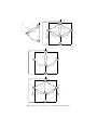
consistency by reasoning directly on the constraint hypergraph. As an illustrative example, consider the lexicographical ordering constraint between two vectors. As shown
by Fig. 1, we come up with an automaton with two states where a transition constraint
corresponds to comparing two domain variables. Now, if we forbid the use of comparison, this would lead to an automaton whose size depends of the number of values in the
domains of the variables.
Our second contribution is to provide for a restricted class of automata an automaton reformulation for the relaxed case. This technique relies on the variable based violation cost introduced in [7, 8]. This cost was advocated as a generic way for expressing
the violation of a global constraint. However, algorithms were only provided for the
soft alldifferent constraint [7]. We come up with an algorithm for computing
a sharp bound of the minimum violation cost and with an automaton reformulation for
pruning in order to avoid to exceed a given maximum violation cost.
Section 2 describes the kind of finite automaton used for recognizing the set of
solutions associated with a global constraint. Section 3 shows how to come up with
an automaton reformulation which exploits the previously introduced automaton. Section 4 describes typical applications of this technique. Finally, for a restricted class of
automata, Section 5 provides a filtering algorithm for the relaxed case.
2 Description of the Automaton Used for Checking Ground
Instances
We first discuss the main issues behind the task of selecting what kind of automaton
to consider for concisely expressing the set of solutions associated with a global constraint. We consider global constraints for which any ground instance can be checked
in linear time by scanning once through their variables without using any data structure. In order to concretely illustrate this point, we first select a set of global constraints
and write down a checker for each of them1 . Observe that a constraint, like for instance the cycle(n, [x1 , x2 , . . . , xm ]) constraint, which enforces that a permutation
[x1 , x2 , . . . , xm ] has n cycles, does not belong to this class since it requires to jump
from one position to another position of the sequence x1 , x2 , . . . , xm . Finally, we give
for each checker a sketch of the corresponding automaton. Based on these observations,
we define the type of automaton we will use.
2.1 Selecting an Appropriate Description
As we previously said, we focus on those global constraints that can be checked by
scanning once through their variables. This is for instance the case of element [9],
minimum [10], pattern [11], global contiguity [12], lexicographic
ordering [13], among [14] and inflexion [15]. Since they illustrate key points
needed for characterizing the set of solutions associated with a global constraint, our
discussion will be based on the last four constraints for which we now recall the definition:
– The global contiguity(vars) constraint enforces for the sequence of 0-1
variables vars to have at most one group of consecutive 1. For instance, the constraint global contiguity([0, 1, 1, 0]) holds since we have only one group of
consecutive 1.
−
−
−
– The lexicographic ordering constraint →
x ≤lex→
y over two vectors of variables →
x =
→
−
hx0 , . . . , xn−1 i and y = hy0 , . . . , yn−1 i holds iff n = 0 or x0 < y0 or x0 = y0
and hx1 , . . . , xn−1 i≤lex hy1 , . . . , yn−1 i.
– The among(nvar , vars, values) constraint restricts the number of variables of the
sequence of variables vars that take their value from a given set values to be equal
to the variable nvar . For instance, among(3, [4, 5, 5, 4, 1], [1, 5, 8]) holds since exactly 3 values of the sequence 45541 are in {1, 5, 8}.
– The inflexion(ninf , vars) constraint enforces the number of inflexions of the
sequence of variables vars to be equal to the variable ninf . An inflexion is
described by one of the following patterns: a strict increase followed by a strict
decrease or, conversely, a strict decrease followed by a strict increase. For instance,
inflexion(4, [3, 3, 1, 4, 5, 5, 6, 5, 5, 6, 3]) holds since we can extract from the
sequence 33145565563 the four subsequences 314, 565, 6556 and 563, which all
follow one of these two patterns.
1
We don’t skip the checker since, in the long term, we consider that the goal would be to turn
any existing code performing a check into a constraint.
global_contiguity
global_contiguity(vars[0..n−1]):BOOLEAN
1 BEGIN
2 i=0;
3 WHILE i<n AND vars[i]=0 DO i++;
vars[i]=0
s
4 WHILE i<n AND vars[i]=1 DO i++;
vars[i]=1
5 WHILE i<n AND vars[i]=0 DO i++;
x[i]=y[i]
6 RETURN (i=n);
7 END.
(A1)
n
< lex(x[0..n−1],y[0..n−1]):BOOLEAN
1 BEGIN
2 i=0;
3 WHILE i<n AND x[i]=y[i] DO i++;
4 RETURN (i=n OR x[i]<y[i]);
5 END.
(B1)
s:
c=0
vars[i]
notin values
$
$
x[i]<y[i]
$
vars[i]=0
t:
t
$
(A2)
nvar=c
(C2)
(B2)
inflexion
vars[i]=vars[i+1]
vars[i]<vars[i+1]
inflexion (ninf,vars[0..n−1]):BOOLEAN
01 BEGIN
02 i=0; c=0;
03 WHILE i<n−1 AND vars[i]=vars[i+1] DO i++;
04 IF i<n−1 THEN less=(vars[i]<vars[i+1]);
05 WHILE i<n−1 DO
06
IF less THEN
07
IF vars[i]>vars[i+1] THEN c++; less=FALSE;
08
ELSE
09
IF vars[i]<vars[i+1] THEN c++; less=TRUE;
10
i++;
11 RETURN (ninf=c);
12 END.
(D1)
s
t
among(nvar,vars[0..n−1],values):BOOLEAN
1 BEGIN
2 i=0; c=0;
3 WHILE i<n DO
4
IF vars[i] in values THEN c++;
5
i++;
6 RETURN (nvar=c);
7 END.
(C1)
z
among
vars[i]
in values,
c++
vars[i]=1
vars[i]=0
$
< lex
vars[i]<
vars[i+1]
s:
vars[i]>
vars[i+1]
vars[i]>
vars[i]>vars[i+1], vars[i+1]
c++
c=0
i
j
vars[i]<vars[i+1],
c++
vars[i]=
vars[i]=
vars[i+1]
vars[i+1]
$
$
t:
$
ninf=c
(D2)
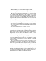
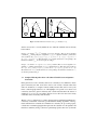
Fig. 1. Four checkers and their corresponding automata.
Parts (A1), (B1), (C1) and (D1) of Fig. 1 depict the four checkers respectively associated
with global contiguity, ≤lex , among and inflexion2. For each checker we
observe the following facts:
– Within the checker depicted by part (A1) of Fig. 1, the values of the sequence
vars[0], . . . , vars[n − 1] are successively compared against 0 and 1 in order to
check that we have at most one group of consecutive 1. This can be translated to
the automaton depicted by part (A2) of Fig. 1. The automaton takes as input the
sequence vars[0], . . . , vars[n − 1], and triggers successively a transition for each
term of this sequence. Transitions labeled by 0, 1 and $ are respectively associated
with the conditions vars[i] = 0, vars[i] = 1 and i = n. Transitions leading to
failure are systematically skipped. This is why no transition labeled with a 1 starts
from state z.
−
– Within the checker given by part (B1) of Fig. 1, the components of vectors →
x
→
−
and y are scanned in parallel. We first skip all the components that are equal and
then perform a final check. This is represented by the automaton depicted by part
(B2) of Fig. 1. The automaton takes as input the sequence hx[0], y[0]i, . . . , hx[n −
1], y[n − 1]i and triggers a transition for each term of this sequence. Unlike the
global contiguity constraint, some transitions now correspond to a condition (e.g. x[i] = y[i], x[i] < y[i]) between two variables of the ≤lex constraint.
– Observe that the among(nvar , vars, values) constraint involves a variable nvar
whose value is computed from a given collection of variables vars. The checker depicted by part (C1) of Fig. 1 counts the number of variables of vars[0], . . . , vars[n−
1] that take their value from values. For this purpose it uses a counter c, which is
eventually tested against the value of nvar . This convinced us to allow the use of
counters in an automaton. Each counter has an initial value which can be updated
while triggering certain transitions. The final state of an automaton can enforce a
variable of the constraint to be equal to a given counter. Part (C2) of Fig. 1 describes
the automaton corresponding to the code given in part (C1) of the same figure. The
automaton uses the counter c, initially set to 0, and takes as input the sequence
vars[0], . . . , vars[n − 1]. It triggers a transition for each variable of this sequence
and increments c when the corresponding variable takes its value in values. The
final state returns a success when the value of c is equal to nvar . At this point we
want to stress the following fact: It would have been possible to use an automaton
that avoids the use of counters. However, this automaton would depend on the effective value of the parameter nvar . In addition, it would require more states than
the automaton of part (C2) of Fig. 1. This is typically a problem if we want to have
a fixed number of states in order to save memory as well as time.
– As the among constraint, the inflexion(ninf , vars) constraint involves a
variable ninf whose value is computed from a given sequence of variables
vars[0], . . . , vars[n − 1]. Therefore, the checker depicted in part (D1) of Fig. 1
also uses a counter c for counting the number of inflexions, and compares its final
value to the ninf parameter. This program is represented by the automaton depicted
2
Within the corresponding automata depicted by parts (A2), (B2), (C2) and (D2) of Fig. 1, we
assume that firing a transition increments from 1 the counter i.
by part (D2) of Fig. 1. It takes as input the sequence of pairs hvars[0], vars[1]i,
hvars[1], vars[2]i , . . . , hvars[n − 2], vars[n − 1]i and triggers a transition for each
pair. Observe that a given variable may occur in more than one pair. Each transition
compares the respective values of two consecutive variables of vars[0..n − 1] and
increments the counter c when a new inflexion is detected. The final state returns a
success when the value of c is equal to ninf .
Synthesizing all the observations we got from these examples leads to the following
remarks and definitions for a given global constraint C:
– For a given state, if no transition can be triggered, this indicates that the constraint
C does not hold.
– Since all transitions starting from a given state are mutually incompatible, all automata are deterministic. Let M denote the set of mutually incompatible conditions
associated with the different transitions of an automaton.
– Let ∆0 , . . . , ∆m−1 denote the sequence of sequences of variables of C on which the
transitions are successively triggered. All these subsets contain the same number of
elements and refer to some variables of C. Since these subsets typically depend on
the constraint, we leave the computation of ∆0 , . . . , ∆m−1 outside the automaton.
To each subset ∆i of this sequence corresponds a variable Si with an initial domain
ranging over [min, min + |M| − 1], where min is a fixed integer. To each integer
of this range corresponds one of the mutually incompatible conditions of M. The
sequences S0 , . . . , Sm−1 and ∆0 , . . . , ∆m−1 are respectively called the signature
and the signature argument of the constraint. The constraint between S i and the
variables of ∆i is called the signature constraint and is denoted by ΨC (Si , ∆i ).
– From a pragmatic point the view, the task of writing a constraint checker is naturally done by writing down an imperative program where local variables (i.e.,
counters), assignment statements and control structures are used. This suggested us
to consider deterministic finite automata augmented with counters and assignment
statements on these counters. Regarding control structures, we did not introduce
any extra feature since the deterministic choice of which transition to trigger next
seemed to be good enough.
– Many global constraints involve a variable whose value is computed from a given
collection of variables. This convinced us to allow the final state of an automaton
to optionally return a result. In practice, this result corresponds to the value of a
counter of the automaton in the final state.
2.2 Defining an Automaton
An automaton A of a constraint C is defined by a sextuple
hSignature, SignatureDomain, SignatureArg, Counters, States, T ransitionsi
where:
– Signature is the sequence of variables S0 , . . . , Sm−1 corresponding to the signature of the constraint C.
– SignatureDomain is an interval which defines the range of possible values of the
variables of Signature.
– SignatureArg is the signature argument ∆0 , . . . , ∆m−1 of the constraint C. The
link between the variables of ∆i and the variable Si (0 ≤ i < m) is done by
writing down the signature constraint ΨC (Si , ∆i ) in such a way that arc-consistency
is maintained. In our context this is done by using standard features of the CLP(FD)
solver of SICStus Prolog [16] such as arithmetic constraints between two variables,
propositional combinators or the global constraints programming interface.
– Counters is the, possibly empty, list of all counters used in the automaton A. Each
counter is described by a term t(Counter , InitialValue, FinalVariable) where
Counter is a symbolic name representing the counter, InitialValue is an integer
giving the value of the counter in the initial state of A, and FinalVariable gives the
variable that should be unified with the value of the counter in the final state of A.
– States is the list of states of A, where each state has the form source(id ), sink(id )
or node(id ). id is a unique identifier associated with each state. Finally, source(id )
and sink(id ) respectively denote the initial and the final state of A.
– T ransitions is the list of transitions of A. Each transition t has the form
arc(id 1 , label , id 2 ) or arc(id 1 , label , id 2 , counters). id 1 and id 2 respectively correspond to the state just before and just after t, while label depicts the value that the
signature variable should have in order to trigger t. When used, counters gives for
each counter of Counters its value after firing the corresponding transition. This
value is specified by an arithmetic expression involving counters, constants, as well
as usual arithmetic functions such as +, −, min or max. The order used in the
counters list is identical to the order used in Counters.
Example 1. As an illustrative example we give the description of the automaton associated with
the inflexion(ninf , vars) constraint. We have:
–
–
–
–
–
–
Signature = S0 , S1 , . . . , Sn−2 ,
SignatureDomain = 0..2,
SignatureArg = hvars[0], vars[1]i, . . . , hvars[n − 2], vars [n − 1]i,
Counters = t(c, 0, ninf ),
States = [source(s), node(i), node(j), sink (t)],
T ransitions = [arc(s, 1, s), arc(s, 2, i), arc(s, 0, j), arc(s, $, t), arc(i, 1, i), arc(i, 2, i),
arc(i, 0, j, [c + 1]), arc(i, $, t), arc(j, 1, j), arc(j, 0, j), arc(j, 2, i, [c + 1]), arc(j, $, t)].
The signature constraint relating each pair of variables hvars[i], vars[i + 1]i to the signature
variable Si is defined as follows: Ψinflexion (Si , vars[i], vars [i+1]) ≡ vars[i] > vars[i+1] ⇔
Si = 0 ∧ vars [i] = vars[i + 1] ⇔ Si = 1 ∧ vars[i] < vars [i + 1] ⇔ Si = 2. The sequence
of transitions triggered on the ground instance inflexion(4, [3, 3, 1, 4, 5, 5, 6, 5, 5, 6, 3]) is
s
c=0
3=3⇔S =1
3>1⇔S =0
1<4⇔S =2
4<5⇔S =2
5=5⇔S =1
5<6⇔S =2
0
1
2
3
4
5
−−−−−−
−→ s −−−−−−
−→ j −−−−−−
−→ i −−−−−−
−→ i −−−−−−
−→ i −−−−−−
−→
6>5⇔S =0
5=5⇔S =1
c=1
5<6⇔S8 =2
6>3⇔S9 =0
$
6
7
i −−−−−−
−→ j −−−−−−
−→ j −−−−−−−→ i −−−−−−−→ j −
→
c=2
c=3
c=4
t
.
ninf =4
Each transition gives the
corresponding condition and, eventually, the value of the counter c just after firing that transition.
3 Automaton Reformulation
The automaton reformulation is based on the following idea. For a given global constraint C, one can think of its automaton as a procedure that repeatedly maps a current
→
−
state Qi and counter vector K i , given a signature variable Si , to a new state Qi+1
→
−
and counter vector K i+1 , until a terminal state is reached. We then convert this pro→
−
→
−
cedure into a transition constraint ΦC (Qi , K i , Si , Qi+1 , K i+1 ) as follows. Qi is a
variable whose values correspond to the states that can be reached at step i. Simi→
−
larly, K i is a vector of variables whose values correspond to the potential values of
the counters at step i. Assuming that the automaton associated with C has na arcs
→
− →
−→ →
−
−
0
arc(q1 , s1 , q10 , f1 ( K )), . . . , arc(qna , sna , qna
, fna ( K )), the transition constraint has
the following form:
na
_
j=1
→
− →
→
−
−
[(Qi = qj ) ∧ (Si = sj ) ∧ (Qi+1 = qj0 ) ∧ ( K i+1 = fj ( K i ))]
Consider first the case when no counter is used, i.e. the constraint is effectively
ΦC (Qi , Si , Qi+1 ). This can be encoded with a ternary relation defined by extension (e.g.
SICStus Prolog’s case [16, page 463], ECLiPSe’s Propia [17], or Ilog Solver’s table
constraint [18]). If that relation maintains arc-consistency, as does case, it follows that
ΦC maintains arc-consistency.
Consider now the case when one counter is used. Then we need to extend the ternary
relation by one argument corresponding to j. This argument can be used as an index
→
− →
−→ →
−
−
→
−
into a vector [ f1 ( K i ), . . . , fna ( K i )], selecting the value that K i+1 should equal. Thus
to encode ΦC we need:
– a 4-ary relation defined by extension,
– na arithmetic constraints to compute the vector, and
– an element constraint to select a value from the vector.
→
− →
−
As an optimization, identical fj ( K i ) expressions can be merged, yielding a shorter vector and fewer arithmetic constraints. In general, arc-consistency can not be guaranteed
for ΦC .
Finally, consider the case when two or more counters are used. This is a straightforward generalization of the single counter case.
We can then arrive at an automaton reformulation for C by decomposing it into a
conjunction of ΦC constraints, “threading” the state and counter variables through the
conjunction. In addition to this, we need the signature constraints Ψ C (Si , ∆i ) (0 ≤
i < m) that relate each signature variables Si to the variables of its corresponding
signature argument ∆i . Filtering for the constraint C is provided by the conjunction
of all signature and transitions constraints, (s being the start state and t being the end
state):
→
−
→
−
ΨC (S0 , ∆0 )
∧ ΦC (s, K 0 , S0 , Q1 , K 1 ) ∧
→
−
→
−
ΨC (S1 , ∆1 )
∧ ΦC (Q1 , K 1 , S1 , Q2 , K 2 ) ∧
.
.
.
→
−
→
−
ΨC (Sm−1 , ∆m−1 ) ∧ ΦC (Qm−1 , K m−1 , Sm−1 , Qm , K m ) ∧
→
−
→
−
ΦC (Qm , K m , $, t, K m+1 )
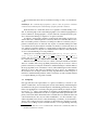
A couple of examples will help clarify this idea. In these examples, the relation
defined by extension is depicted in a compact form as a decision tree. Note that the
automaton
decision tree
automaton
decision tree
1,c++
s
2
Qi=s
s:
Qi=t
Qi=t
Qi=s
c=0
0
1
$
t
Si=1
Si=$
$
Si=2
Qi+1=s
(A)
Si=$
Si=0
Qi+1=t
t:
nvar=c
Si=1
Qi+1=s
Qi+1=s
Qi+1=t
ci+1=ci
ci+1=ci+1
ci+1=ci
(B)
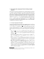
Fig. 2. Automata and decision trees for (A) ≤lex and (B) among.
decision tree needs to correctly handle the case when the terminal state has already
been reached.
−
−
Example 2. Consider a →
x ≤lex →
y constraint over vectors of length n. First, we need a signature
constraint Ψ≤lex relating each pair of arguments x[i], y[i] to a signature variable Si . This can be
done as follows: Ψ≤lex (Si , x[i], y[i]) ≡ (x[i] < y[i] ⇔ Si = 1) ∧ (x[i] = y[i] ⇔ Si =
2) ∧ (x[i] > y[i] ⇔ Si = 3). The automaton of ≤lex and the decision tree corresponding to the
transition constraint Φ≤lex are shown in part (A) of Fig. 2.
Example 3. Consider a among(nvar , vars, values) constraint. First, we need a signature constraint Ψamong relating each argument vars[i] to a signature letter Si . This can be done as follows:
Ψamong (Si , vars[i], values) ≡ (vars [i] ∈ values ⇔ Si = 1) ∧ (vars [i] 6∈ values ⇔ Si = 0).
The automaton of among and the decision tree corresponding to the transition constraint Φamong
are shown in part (B) of Fig. 2.
3.1 Complete Filtering when there is No Shared Variable between Signature
Constraints
In the general case, local consistency such as arc-consistency is not sufficient to ensure
global consistency. In other words, there can be some locally consistent values that
cannot be extended to a complete solution, mainly because there can be some cycles
in the constraint graph. However, we will highlight some special cases where local
consistency can lead to global consistency: We consider automata where all subsets of
variables in SignatureArg are pairwise disjoint. As we will see in the section, many
constraints can be encoded by such automata.
Without counters. If there are no counters, the automaton reformulation maintains arcconsistency on this kind of automata, provided that the filtering algorithms of the signature and transition constraints also maintain arc-consistency. To prove this property,
consider the constraint hypergraph that represents the conjunction of all signature and
transition constraints (see Fig. 3). It has two particular properties: there is no cycle in the
corresponding dual graph [19]3 , and for any pair of constraints the two sets of involved
variables share at most one variable. Such a hypergraph is so-called Berge-acyclic [21].
Berge-acyclic constraint networks were proved to be solvable polynomially by achiev-
s
X0
X1
X m−1
Y0
...
Y1
...
Y m−1
...
S0
S1
S m−1
Q1
Q2
Q m−1
$
Qm
t
Fig. 3. Constraint hypergraph of the conjunction of transition and signature constraints in the case
of disjoint SignatureArg sets. The i-th SignatureArg set ∆i is denoted by {Xi , Yi , . . .}.
ing arc-consistency [22, 23]. Therefore, if all signature and transition constraints maintain arc-consistency then we obtain a complete filtering for our global constraint.
Among the 39 constraints studied in [24], eight (between,
between exactly one,
global contiguity,
lex different,
lex lesseq,
pattern,
two quad are in contact,
and
two quad do not overlap) have an automaton leading to a Berge-acyclic
hypergraph.
With counters. If there are counters, some pairs of constraints share more than one
variable. So, the hypergraph is not Berge-acyclic and the filtering performed may be no
longer optimal. However, achieving pairwise consistency on some pairs of constraints
leads to a complete filtering. To prove this, we will use the following well-know theorem
in database systems.
Definition 1. [25] A constraint network N = {X , D, C} is pairwise consistent if and
only if ∀Ci ∈ C, Ci 6= ∅ and ∀Ci , Cj ∈ C, Ci |s = Cj |s where s is the set of variables
shared by Ci and Cj and Ci |s is the projection of Ci on s.
Definition 2. [26] An edge in the dual graph of a constraint network is redundant if
its variables are shared by every edge along an alternative path between the two end
points. The subgraph resulting from the removal of the redundant edges of the dual
graph is called a join graph. A hypergraph has a join tree if its join graph is a tree.
Theorem 1. [25] A database scheme is α-acyclic[27] if and only if its hypergraph has
a join tree.
Theorem 2. [25] Any pairwise consistent database over an α-acyclic database scheme
is globally consistent.
3
To each constraint corresponds a node in the dual graph and if two constraints have a nonempty
set S of shared variables, then there is an edge labelled S between their corresponding nodes
in the dual graph. The dual graph is also called intersection graph in data base theory [20].
If we translate these theorems we obtain the following corollary on constraint networks.
Corollary 1. If a constraint hypergraph has a join tree then any pairwise consistent
constraint network having this constraint hypergraph is globally consistent.
In the automata we consider here, there are no signature constraints sharing a variable. So, the dual graph of the constraint hypergraph is a tree and the hypergraph has a
join tree. Therefore, the hypergraph is α-acyclic and if the constraint network is pairwise consistent, the filtering is complete for our global constraint.
A solution to reach global consistency on the network representing our global constraint is therefore to maintain pairwise consistency. In fact, if constraints share no more
than one variable, pairwise consistency is nothing more than arc-consistency [23]. So,
pairwise consistency has to be enforced only on pairs of constraints sharing more than
one variable and only the transition constraints are therefore concerned. In the worst
case, pairwise consistency will have to consider all the possible tuples of values for the
set of shared variables. So, the pairs of constraints must not share too many variables if
we do not want the filtering to become prohibitive.
Among the 39 constraints studied in [24], seven (among, atleast, atmost,
count, counts, differ from atleast k pos, and sliding card skip0)
require only one counter, two (group, and group skip isolated item) need
two counters and max index requires three counters.
When the automaton involves only one counter, consecutive transition constraints
share two variables. The sweep algorithm presented in [28] can be used to enforce
pairwise consistency on each pair of transition constraints sharing two variables. Indeed,
the sweep algorithm on two constraints Ci and Cj will forbid the tuples for the variables
shared by Ci and Cj that cannot be extended on both Ci and Cj . To summarize, if
the automaton uses one single counter, the sweep algorithm must consider each pair of
transition constraints sharing variables, and arc-consistency on each constraint will lead
to a complete filtering for our global constraint.
3.2 Complexity
Our approach allows the representation of a global constraint by a network of constraints of small arities. As seen in the previous section, the filtering obtained using this
reformulation of the global constraint depends on the filtering performed by the solver.
If the solver maintains arc-consistency using the general schema [29, 30], the complexity is in O(er2 dr ) 4 where e is the number of constraints, r the maximum arity and d the
size of the largest domain. However, this is a rough bound and the practical time complexity can be far from this limit. Indeed, the constraints have very different arities and
some domains involve only very few values. Furthermore, on some constraints a specialized algorithm can be used to reduce the filtering cost. Finally, one would want to
enforce only a partial form of arc-consistency (a directional arc-consistency for example in the case of a Berge-acyclic constraint network), or a stronger filtering (enforcing
4
We assume here that the cost of a constraint check is linear in the constraint arity while it is
sometimes assumed to be constant.
pairwise consistency for example on a constraint network having a join tree). Both the
pruning efficiency and the complexity of the pruning rely on the filtering performed by
the solver.
3.3 Performance
It is reasonable to ask the question whether the automaton reformulation described
herein performs anywhere near the performance delivered by a specific implementation of a given constraint. To this end, we have compared a version of the Balanced
Incomplete Block Design problem [31, prob028] that uses a built-in ≤ lex constraint to
break column symmetries with a version using our filtering based on a finite automaton
for the same constraint. In a second experiment, we measured the time to find all solutions to a single ≤lex constraint. The experiments were run in SICStus Prolog 3.11 on
a 600MHz Pentium III. The results are shown in Table 1.
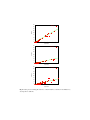
A third experiment was designed to measure the overhead of an automaton reformulation wrt. decomposing into built-in constraints. To this end, we produced random instances of the following constraints studied in [24]: among, between, lex lesseq.
These constraints were chosen because their automata formulations maintain the same
consistency as their decomposed formulations, that is, they perform exactly the same
domain filtering. Hence, comparing the time it takes to compute all solutions should
give an accurate measurement of the overhead. among is not a built-in constraint; it
can be decomposed into a number of reified membership constraints and a sum constraint. It is worth noting that its automaton uses a counter. between, lex lesseq
can be expressed as built-in lex chain constraints. The results are presented in three
scatter plots in Figure 4. Each graph compares times for finding all solutions to a random constraint instance, using a randomly chosen labeling strategy. The X coordinate
of each point is the runtime for an automaton reformulation. The Y coordinate is the
runtime for a decomposition into built-in constraints. A line, least-square fitted to the
data points, is shown in each graph. Runtimes are in seconds.
From these experiments, we observe that an automaton reformulation typically runs
a few times slower than its hard-coded counterpart, roughly the same ratio as between
interpreted and compiled code in a typical programming language. This slowdown is
likely to have much less impact on the overall execution time of the program. The
conclusion is that the automaton reformulation is a feasible and very reasonable way of
rapidly prototyping new global constraints, before embarking on developing a specific
filtering algorithm, should that be deemed necessary.
4 Applications of this Technique
4.1 Designing Automaton Reformulations for Global Constraints
We apply this new methodology for designing automaton reformulations for the following fairly large set of global constraints. We came up with an automaton 5 for the
following constraints:
5
These automata are available in the technical report [24]. All signature constraints are encoded
in order to maintain arc-consistency.
40
among
35
30
built-in
25
20
15
10
5
0
0
5
10
15
20
25
30
35
40
35
40
35
40
automaton
40
between
35
30
built-in
25
20
15
10
5
0
0
5
10
15
20
25
30
automaton
40
lex_lesseq
35
30
built-in
25
20
15
10
5
0
0
5
10
15
20
25
30
automaton
Fig. 4. Scatter plots for finding all solutions to random instances: automaton reformulation vs.
decomposition to built-ins.
Table 1. Time in milliseconds for finding (A) the first solution of BIBD instances using built-in
vs. simulated ≤lex (BCS denotes time spent for breaking column symmetries: with respect to
the first column, BCS corresponds to the time spent in the built-in ≤lex constraint), and (B) all
solutions to a single built-in vs. simulated ≤lex constraint.
(A)
Problem
Built-in ≤lex Simulated ≤lex
v, b, r, k, λ
BCS/Other
BCS/Other
6, 50, 25, 3, 10
70/170
250/170
6, 60, 30, 3, 12
120/110
50/110
8, 14, 7, 4, 3
10/80
50/80
9, 120, 40, 3, 10 480/1090
440/1090
10, 90, 27, 3, 6
550/90
1010/90
10, 120, 36, 3, 8 1400/2070
1040/2070
12, 88, 22, 3, 4
450/970
530/970
13, 104, 24, 3, 4 540/1230
540/1230
15, 70, 14, 3, 2
220/910
520/910
(B)
xi ∈ [0, m − 1], yi = m − i
−
−
|→
x | = |→
y|=m
m Built-in ≤lex Simulated ≤lex
4
10
20
5
110
170
6
1640
2300
7
29530
39100
– Unary constraints specifying a domain like in [32] or not in [33].
– Channeling constraints like domain constraint [34].
– Counting constraints for constraining the number of occurrences of a given set of
values like among [14], atleast [33], atmost [33] or count [32].
– Sliding sequence constraints like change
[35], longest change or
smooth [15]. longest change(size, vars, ctr ) restricts the variable size to the
maximum number of consecutive variables of vars for which the binary constraint
ctr holds.
– Variations around the element constraint [9] like element greatereq [36],
element lesseq [36] or element sparse [33].
– Variations around the maximum constraint [10] like max index(vars, index ).
max index enforces the variable index to be equal to one of the positions of
variables corresponding to the maximum value of the variables of vars.
– Constraints on words like global contiguity [12], group [33],
group skip isolated item [15] or pattern [11].
– Constraints between vectors of variables like between [1], ≤lex [13],
lex different or differ from at least k pos. Given two vectors
→
−
−
x and →
y which have the same number of components, the constraints
−
−
−
−
lex different(→
x,→
y ) and differ from at least k pos(k, →
x,→
y ) re→
−
→
−
spectively enforce the vectors x and y to differ from at least 1 and k components.
– Constraints between n-dimensional boxes like two quad are in contact [33]
or two quad do not overlap [37].
– Constraints on the shape of a sequence of variables like inflexion [15], top [38]
or valley [38].
– Various constraints like in same partition(var 1 , var 2 , partitions),
not all equal(vars) or sliding card skip0(atleast, atmost, vars, values).
in same partition enforces variables var 1 and var 2 to be respectively assigned to two values that both belong to a same sublist of values of partitions.
not all equal enforces the variables of vars to take more than a single value.
sliding card skip0 enforces that each maximum non-zero subsequence of
consecutive variables of vars contain at least atleast and at most atmost values
from the set of values values.
4.2 Automaton Reformulation for a Conjunction of Global Constraints
Another typical use of our new methodology is to come up with an automaton reformulation for the conjunction of several global constraints. This is usually difficult
since it implies analyzing a lot of special cases showing up from the interaction of
the different considered constraints. We illustrate this point on the conjunction of the
→
−
−
−
−
between(→
a ,→
x , b ) [1] and the exactly one(→
x , values) constraints for which
we come up with an automaton reformulation, which maintains arc-consistency. The
→
−
−
−
−
between constraint holds iff →
a ≤lex →
x and →
x ≤lex b , while the exactly one con−
straint holds if exactly one component of →
x takes its value in the set of values values.
The left-hand part of Fig. 5 depicts the two automata A1 and A2 respectively associated with the between and the exactly one constraints, while the right-hand
part gives the automaton A3 associated with the conjunction of these two constraints.
A3 corresponds to the product of A1 and A2 . States of A3 are labeled by the two states
of A1 and A2 they were issued. Transitions of A3 are labeled by the end symbol $ or
by a conjunction of elementary conditions, where each condition is taken in one of the
following set of conditions {ai < xi , ai = xi , ai > xi }, {bi > xi , bi = xi , bi < xi },
{xi ∈ values, xi 6∈ values}. This makes up to 3 · 3 · 2 = 18 possible combinations and
leads to the signature constraint Ψbetween∧exactly one (Si , ai , xi , bi , values) between
→
−
−
−
the signature variable Si and the i-th component of vectors →
a,→
x and b :
8
0
>
>
>
>
>
1
>
>
>
>
2
>
>
>
>
>
<3
Si = 4
>
>
>
5
>
>
>
>
>6
>
>
>
>
7
>
>
:
8
if ai
if ai
if ai
if ai
if ai
if ai
if ai
if ai
if ai
<
<
<
=
=
=
>
>
>
xi
xi
xi
xi
xi
xi
xi
xi
xi
∧ bi
∧ bi
∧ bi
∧ bi
∧ bi
∧ bi
∧ bi
∧ bi
∧ bi
> x i ∧ xi
= xi ∧ xi
< x i ∧ xi
> x i ∧ xi
= xi ∧ xi
< x i ∧ xi
> x i ∧ xi
= xi ∧ xi
< x i ∧ xi
6∈ values,
6∈ values,
6∈ values,
6 values,
∈
6 values,
∈
6∈ values,
6∈ values,
6∈ values,
6∈ values,
9
10
11
12
13
14
15
16
17
if ai
if ai
if ai
if ai
if ai
if ai
if ai
if ai
if ai
< x i ∧ bi
< x i ∧ bi
< x i ∧ bi
= x i ∧ bi
= x i ∧ bi
= x i ∧ bi
> x i ∧ bi
> x i ∧ bi
> x i ∧ bi
> x i ∧ xi
= xi ∧ xi
< x i ∧ xi
> x i ∧ xi
= xi ∧ xi
< x i ∧ xi
> x i ∧ xi
= xi ∧ xi
< x i ∧ xi
∈ values,
∈ values,
∈ values,
∈ values,
∈ values,
∈ values,
∈ values,
∈ values,
∈ values.
→
−
−
−
In order to maintain arc-consistency on the conjunction of the between( →
a ,→
x, b)
−
and the exactly one(→
x , values) constraints we need to have arc-consistency on
Ψbetween∧exactly one (Si , ai , xi , bi , values). In our context this is done by using the
global constraint programming facilities of SICStus Prolog [32]6 .
Example 4. Consider three variables x ∈ {0, 1}, y ∈ {0, 3}, z ∈ {0, 1, 2, 3} subject to the conjunction of constraints between(h0, 3, 1i, hx, y, zi, h1, 0, 2i) ∧ exactly one(hx, y, zi, {0}).
Even if both the between and the exactly one constraints maintain arc-consistency, we need
the automaton associated with their conjunction to find out that z 6= 0. This can be seen as follows: after two transitions, the automaton A3 will be either in state ai or in state bi. However,
in either state, a 0 must already have been seen, and so there is no support for z = 0.
6
The corresponding code is available in the technical report [24].
between
exactly_one
between and exactly_one
eEO
e
lE
E
b
eE
o
O
eEI
eo
eEO
ei
eLI
I
eL
e
a
l
$
L
$
t
lL
$
i
lEO
lEO
$
EO
bo
ao
eO
eLO
lLI
eLO
O
lEI
bi
lLO
EO
ai
eO
lLO
lO
t
LO
LEGEND
l: ai<xi L: bi>xi I: xi in values
e: ai=xi E: bi=xi O: xi not in values
g: ai>xi G: bi<xi $: end
LO
O
O
to
ti
lO
$
I
LI
lI
EI
$
$
$
tt
eI
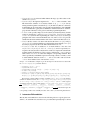
Fig. 5. Automata associated with between and exactly one and the automaton associated
with their conjunction.
4.3 Designing Constraints between Two Sequences of Variables
This section considers constraints of the form C(N, [VAR 1 , VAR2 , . . . , VARm ]) for
which the corresponding automaton AC uses one single counter, which is incremented
by certain transitions and finally unified to variable N in the final state of A C . This
corresponds to constraints that count the number of occurrences of a given pattern in a
sequence VAR1 VAR2 . . . VARm . Each time the automaton recognizes a pattern in the
sequence, it increments its counter by +1. Given the automaton A C of such a constraint
C we will show how to create the automata associated to the following constraints:
– synchronizedC ([U1 , U2 , . . . , Um ], [V1 , V2 , . . . , Vm ]) enforces that all positions
where the automaton AC recognizes a pattern in U1 U2 . . . Um correspond exactly
to the positions where AC recognizes a pattern in V1 V2 . . . Vm . In other words the
positions where both counters are incremented should coincide in both sequences.
– distinctC ([U1 , U2 , . . . , Um ], [V1 , V2 , . . . , Vm ]) enforces that all positions where the
automaton AC recognizes a pattern in U1 U2 . . . Um be distinct from all positions
where AC recognizes a pattern in V1 V2 . . . Vm . This means that the positions where
a counter is incremented should all be distinct.
As an illustrative example, consider the peak constraint, which counts the number of peaks of a sequence of variables where adjacent variables are not equal. The
automaton of this constraint is depicted by part (A) of Fig. 6.
We explain how to derive the automaton associated to synchronizedC and to
distinctC from the automaton AC associated to C. Let A2C , S(AC ) and D(AC ) respectively denotes the automaton that is the product of AC and AC , the automaton
associated to synchronizedC , and the automaton associated to distinct C . Regarding
the example of the peak constraint A2C is given by part (B) of Fig. 6.
We compute S(AC ) and D(AC ) from A2C . Within A2C we partition its transitions
into the following 4 classes:
Ui >Ui+1 ,Vi >Vi+1
ss:
(B)
(A)
VAR i>VAR i+1
s:
C=0
Ui <Ui+1 ,
Vi >Vi+1
us
VAR i<VAR i+1
VAR i>VAR i+1,
{C=C+1}
VAR i<VAR i+1
u
Ui >Ui+1 ,
Vi >Vi+1 ,
{C=C+1}
Ui >Ui+1 ,
Vi >Vi+1 ,
Ui >Ui+1 ,
Ui >Ui+1 , {D=D+1}
Vi <Vi+1
Vi >Vi+1 ,
{C=C+1,D=D+1}
su
U >U
,
i i+1
Ui <Ui+1 ,
Vi <Vi+1 ,
Vi >Vi+1 ,
{C=C+1}
U <U
,
i i+1
V <V
i i+1
Ui <Ui+1 ,
Vi >Vi+1 ,
{D=D+1}
Ui >Ui+1 ,
Vi <Vi+1 ,
$
C=D=0 U >U
i i+1 ,Vi <Vi+1
Ui <Ui+1 ,Vi >Vi+1
{C=C+1}
uu
Ui <Ui+1 ,
Vi <Vi+1
su
Ui <Ui+1 ,
Vi <Vi+1
$
t:
N=C
$
$
{D=D+1}
Ui <Ui+1 ,
Vi <Vi+1
$
t
Ui >Ui+1 ,Vi >Vi+1
(C)
Ui <Ui+1 ,Vi >Vi+1
Ui <Ui+1 ,
Vi >Vi+1
us
ss
U <U
,
i i+1
V <V
i i+1
Ui >Ui+1 ,Vi <Vi+1
su
uu
Ui <Ui+1 ,
Vi <Vi+1
$
$
Ui >Ui+1 ,
Vi <Vi+1
Ui >Ui+1 ,
Vi >Vi+1
Ui <Ui+1 ,
Vi <Vi+1
Ui <Ui+1 ,
Vi <Vi+1
$
$
t
Ui >Ui+1 ,Vi >Vi+1
(D)
Ui <Ui+1 ,Vi >Vi+1
ss
Ui >Ui+1 ,Vi <Vi+1
Ui >Ui+1 ,
Vi >Vi+1 ,
Ui <Ui+1 ,
Vi >Vi+1
us
Ui >Ui+1 ,
Vi >Vi+1 ,
U <U
,
i i+1
V <V
i i+1
su
Ui <Ui+1 ,
Vi >Vi+1 ,
Ui >Ui+1 ,
Vi <Vi+1 ,
U >U
,
i i+1
Vi <Vi+1 ,
uu
Ui <Ui+1 ,
Vi <Vi+1
su
$
$
Ui >Ui+1 ,
Vi <Vi+1
Ui <Ui+1 ,
Vi <Vi+1
$
Ui <Ui+1 ,
Vi >Vi+1 ,
Ui <Ui+1 ,
Vi <Vi+1
us
$
t
Fig. 6. Automaton associated to the peak constraint and derived automata.
us
$
– Those transitions that do not increment any counter,
– Those transitions that only increment the counter associated to the sequence
U1 U2 . . . Um .
– Those transitions that only increment the counter associated to the sequence
V1 V2 . . . V m .
– Finally, those transitions that increment both counters.
S(AC ) corresponds to A2C from which we remove all transitions where only one single
counter is incremented, and D(AC ) corresponds to A2C from which we remove all
transitions where both counters are incremented. We also remove from the resulting
automata all counter variables. Coming back to the example of the peak constraint,
S(AC ) and D(AC ) respectively correspond to part (C) and (D) of Fig. 6.
5 Handling Relaxation for a Counter-Free Automaton
This section presents a filtering algorithm for handling constraint relaxation under the
assumption that we don’t use any counter in our automaton. It can be seen as a generalization of the algorithm used for the regular constraint [6].
Definition 3. The violation cost of a global constraint is the minimum number of subsets of its signature argument for which it is necessary to change at least one variable
in order to get back to a solution.
When these subsets form a partition over the variables of the constraint and when they
consist of a single element, this cost is in fact the minimum number of variables to
unassign in order to get back to a solution. As in [7], we add a cost variable cost as
an extra argument of the constraint. Our filtering algorithm first evaluates the minimum
cost value Min. Then, according to max(cost ), it prunes values that cannot belong to
a solution.
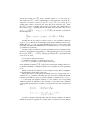
Example 5. Consider the constraint global contiguity([V0 , V1 , V2 , V3 , V4 , V5 , V6 ]) with
the following current domains for variables Vi : [{0, 1}, {1}, {1}, {0}, {1}, {0, 1}, {1}]. The
constraint is violated because there are necessarily at least two distinct sequences of consecutive 1. To get back to a state that can lead to a solution, it is enough to turn
the fourth value to 1. One can deduce Min = 1. Consider now the relaxed form
soft global contiguity([V0 , V1 , V2 , V3 , V4 , V5 , V6 ], cost ) and assume max(cost ) = 1.
The filtering algorithm should remove value 0 from V5 . Indeed, selecting value 0 for variable
V5 entails a minimum violation cost of 2. Observe that for this constraint the signature variables
S0 , S1 , S2 , S3 , S4 , S5 , S6 are V0 , V1 , V2 , V3 , V4 , V5 , V6 .
As in the algorithm of Pesant [6], our consistency algorithm builds a layered acyclic
directed multigraph G. Each layer of G contains a different node for each state of our
automaton. Arcs only appear between consecutive layers. Given two nodes n 1 and n2 of
two consecutive layers, q1 and q2 denote their respective associated state. There is an arc
a from n1 to n2 iff, in the automaton, there is an arc arc(q1 , v, q2 ) from q1 to q2 . The arc
a is labeled with the value v. Arcs corresponding to transitions that cannot be triggered
according to the current domain of the signature variables S0 , . . . , Sm−1 are marked
as infeasible. All other arcs are marked as feasible. Finally, we discard isolated nodes
from our layered multigraph. Since our automaton has a single initial state and a single
final state, G has one source and one sink, denoted by source and sink respectively.
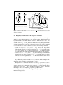
Example 5 continued. Part (A) of Fig. 7 recalls the automaton of the global contiguity
constraint, while part (B) gives the multigraph G associated with the soft global contiguity
constraint previously introduced. Each arc is labeled by the condition associated to its corresponding transition. Each node contains the name of the corresponding automaton state. Numbers in a
node will be explained later on. Infeasible arcs are represented with a dotted line.
s
0
1
n
S
1
0
$
z
S
0
s:0,1
$
0
$
t
(A) Automaton for
global_contiguity
0
S
1
s:0,1
1
n:0,1
0
S
2
s:1,1
0
S
3
s:2,0
0
S
4
s:2,0
0
S
5
s:3,0
0
6
s:3,0
0
1
1
1
1
1
1
1
1
1
1
1
1
n:0,1
0
z:1,3
n:0,1
n:1,0
n:1,0
i:1,0
0
0
0
0
0
0
0
0
0
0
z:1,2
z:0,2
z:1,1
z:1,1
s:4,0
$
n:1,0
$
t:1,0
$
z:2,0
(B) Graph of potential executions of the automaton of
global_contiguity according to S0 ,S1 ,S2 ,S3 ,S4 ,S5 ,S6
Fig. 7. Relaxing the global contiguity constraint.
We now explain how to use the multigraph G to evaluate the minimum violation cost
Min and to prune the signature variables according to the maximum allowed violation
cost max(cost). Evaluating the minimum violation cost Min can be seen as finding
the path from the source to the sink of G that contains the smallest number of infeasible
arcs. This can be done by performing a topological sort starting from the source of G.
While performing the topological sort, we compute for each node n k of G the minimum
number of infeasible arcs from the source of G to nk 7 . This number is recorded in
before[nk ]. At the end of the topological sort, the minimum violation cost Min we
search for, is equal to before[sink ].
Notation 1 Let i be assignable to a signature variable Sl . Min il denotes the minimum
violation cost value according to the hypothesis that we assign i to S l .
To prune domains of signature variables we need to compute the quantity Min il . In
order to do so, we introduce the quantity after [nk ] for a node nk of G: after [nk ] is
the minimum number of infeasible arcs on all paths from nk to sink . It is computed
7
The acyclic graph is layered and no transitive arcs exist. Therefore for each node nk at a given
layer k, the quantity bef ore[nk ] is computed from the nodes of layer k − 1 as follows: for
each nk−1 such that there exists an arc from nk−1 to nk , we add 1 to bef ore[nk−1 ] if it is an
infeasible arc, and 0 if it is a feasible arc. Then bef ore[nk ] is the minimum of such computed
quantities.
by performing a second topological sort starting from the sink of G. Let A il denote
the set of arcs of G, labeled by i, for which the origin has a rank of l. The quantity
min i (before[a] + after [b]) represents the minimum violation cost under the hypoth-
a→b∈Al
esis that Sl remains assigned to i. If that quantity is greater than Min then there is no
path from source to sink that uses an arc of Ail and that has a number of infeasible arcs
equal to Min. In that case the smallest cost we can achieve is Min + 1. Therefore we
have:
Min il = min( min (before[a] + after [b]), Min + 1)
a→b∈Ail
The filtering algorithm is then based on the following theorem:
Theorem 3. Let i be a value from the domain of a signature variable S l . If Min il >
max(cost) then i can be removed from Sl .
The cost of the filtering algorithm is dominated by the two topological sorts. They have
a cost proportional to the number of arcs of G, which is bounded by the number of signature variables times the number of arcs of the automaton.
Example 5 continued. Let us come back to the instance of Fig. 7. Beside the state’s name,
each node nk of part (B) of Fig. 7 gives the values of before[nk ] and of after [nk ]. Since
before[sink ] = 1 we have that the minimum cost violation is equal to 1. Pruning can be potentially done only for signature variables having more than one value. In our example this corresponds to variables V0 and V5 . So we evaluate the four quantities Min 00 = min(0 + 1, 2) = 1,
Min 10 = min(0 + 1, 2) = 1, Min 05 = min(min(3 + 0, 1 + 1, 1 + 1), 2) = 2, Min 15 =
min(min(3 + 0, 1 + 0), 2) = 1. If max(cost ) is equal to 1 we can remove value 0 from V5 . The
corresponding arcs are depicted with a thick line in Fig. 7.
6 Conclusion and Perspectives
The automaton description introduced in this article can be seen as a restricted programming language. This language is used for writing down a constraint checker, which verifies whether a ground instance of a constraint is satisfied or not. This checker allows
pruning the variables of a non-ground instance of a constraint by simulating all potential executions of the corresponding program according to the current domain of the
variables of the relevant constraint. This simulation is achieved by encoding all potential executions of the automaton as a conjunction of signature and transition constraints
and by letting the usual constraint propagation deducing all the relevant information.
We want to stress the key points and the different perspectives of this approach:
– Within the context of global constraints, it was implicitly assumed that providing a
constraint checker is a much easier task than coming up with a filtering algorithm.
It was also commonly admitted that the design of filtering algorithms is a difficult
task, which involves creativity and which cannot be automatized. We have shown
that this is not the case any more if one can afford to provide a constraint checker.
– Non-determinism has played a key role by augmenting programming languages
with backtracking facilities [39], which was the origin of logic programming. Nondeterminism also has a key role to play in the systematic design of filtering algorithms: finding a filtering algorithm can be seen as the task of executing in a nondeterministic way the deterministic program corresponding to a constraint checker
and to extract the relevant information that is common to all execution paths. This
can indeed be achieved by using constraint programming.
– A natural continuation would be to extend the automaton description in order to get
closer to a classical imperative programming language. This would allow the direct
of available checkers in order to systematically get a automaton reformulation.
– Other structural conditions on the signature and transition constraints could be identified to guarantee arc-consistency for the original global constraint.
– An extension of our approach may give a systematic way to get an algorithm (not
necessarily polynomial) for decision problems for which one can provide a polynomial certificate. From [40] the decision version of every problem in NP can be
formulated as follows: Given x, decide whether there exists y so that |y| ≤ m(x)
and R(x, y). x is an instance of the problem; y is a short YES-certificate for this
instance; R(x, y) is a polynomial time decidable relation that verifies certificate y
for instance x; and m(x) is a computable and polynomially bounded complexity
parameter that bounds the length of the certificate y. In our context, if |y| is fixed
and known, x is a global constraint and its |y| variables with their domains; y is a
solution to that global constraint; R(x, y) is an automaton, which encodes a checker
for that global constraint.
Acknowledgments. We are grateful to I. Katriel for suggesting the use of topological sort for the
relaxation part, and to C. Bessière for his helpful comments wrt. Berge-acyclic CSP’s.
References
1. M. Carlsson and N. Beldiceanu. From constraints to finite automata to filtering algorithms.
In D. Schmidt, editor, Proc. ESOP2004, volume 2986 of LNCS, pages 94–108. SpringerVerlag, 2004.
2. N. R. Vempaty. Solving constraint satisfaction problems using finite state automata. In National Conference on Artificial Intelligence (AAAI-92), pages 453–458. AAAI Press, 1992.
3. J. Amilhastre. Représentation par automate d’ensemble de solutions de problèmes de satisfaction de contraintes. PhD Thesis, 1999.
4. J. Amilhastre, H. Fargier, and P. Marquis. Consistency restoration and explanations in dynamic CSPs – application to configuration. Artificial Intelligence, 135:199–234, 2002.
5. B. Boigelot and P. Wolper. Representing arithmetic constraints with finite automata: An
overview. In Peter J. Stuckey, editor, ICLP’2002, Int. Conf. on Logic Programming, volume
2401 of LNCS, pages 1–19. Springer-Verlag, 2002.
6. G. Pesant. A regular language membership constraint for sequence of variables. In Workshop
on Modelling and Reformulation Constraint Satisfaction Problems, pages 110–119, 2003.
7. T. Petit, J.-C. Régin, and C. Bessière. Specific filtering algorithms for over-constrained problems. In T. Walsh, editor, Principles and Practice of Constraint Programming (CP’2001),
volume 2239 of LNCS, pages 451–463. Springer-Verlag, 2001.
8. M. Milano. Constraint and integer programming. Kluwer Academic Publishers, 2004. ISBN
1-4020-7583-9.
9. P. Van Hentenryck and J.-P. Carillon. Generality vs. specificity: an experience with AI and
OR techniques. In National Conference on Artificial Intelligence (AAAI-88), 1988.
10. N. Beldiceanu. Pruning for the minimum constraint family and for the number of distinct
values constraint family. In T. Walsh, editor, CP’2001, Int. Conf. on Principles and Practice
of Constraint Programming, volume 2239 of LNCS, pages 211–224. Springer-Verlag, 2001.
11. S. Bourdais, P. Galinier, and G. Pesant. HIBISCUS: A constraint programming application
to staff scheduling in health care. In F. Rossi, editor, CP’2003, Principles and Practice of
Constraint Programming, volume 2833 of LNCS, pages 153–167. Springer-Verlag, 2003.
12. M. Maher. Analysis of a global contiguity constraint. In Workshop on Rule-Based Constraint
Reasoning and Programming, 2002. held along CP-2002.
13. A. Frisch, B. Hnich, Z. Kızıltan, I. Miguel, and T. Walsh. Global constraints for lexicographic orderings. In Pascal Van Hentenryck, editor, Principles and Practice of Constraint
Programming (CP’2002), volume 2470 of LNCS, pages 93–108. Springer-Verlag, 2002.
14. N. Beldiceanu and E. Contejean. Introducing global constraints in CHIP. Mathl. Comput.
Modelling, 20(12):97–123, 1994.
15. N. Beldiceanu. Global constraints as graph properties on structured network of elementary
constaints of the same type. In R. Dechter, editor, CP’2000, Principles and Practice of
Constraint Programming, volume 1894 of LNCS, pages 52–66. Springer-Verlag, 2000.
16. M. Carlsson et al. SICStus Prolog User’s Manual. Swedish Institute of Computer Science,
3.11 edition, January 2004. http://www.sics.se/sicstus/.
17. T. Le Provost and M. Wallace. Domain-independent propagation. In Proc. of the International Conference on Fifth Generation Computer Systems, pages 1004–1011, 1992.
http://www.icparc.ic.ac.uk/eclipse/.
18. ILOG. ILOG Solver Reference Manual, 6.0 edition. http://www.ilog.com.
19. R. Dechter and J. Pearl. Tree clustering for constraint networks. Artificial Intelligence,
38:353–366, 1989.
20. D. Maier. The Theory of Relational Databases. Computer Science Pres, Rockville, MD,
1983.
21. C. Berge. Graphs and hypergraphs. Dunod, Paris, 1970.
22. P. Janssen and M-C. Vilarem. Problèmes de satisfaction de contraintes: techniques de
résolution et application à la synthèse de peptides. Research Report C.R.I.M., 54, 1988.
23. P. Jégou. Contribution à l’étude des problèmes de satisfaction de contraintes: algorithmes de
propagation et de résolution. Propagation de contraintes dans les réseaux dynamiques. PhD
Thesis, 1991.
24. N. Beldiceanu, M. Carlsson, and T. Petit. Deriving filtering algorithms from constraint
checkers. Technical Report T2004-08, Swedish Institute of Computer Science, 2004.
25. C. Beeri, R. Fagin, D. Maier, and M. Yannakakis. On the desirability of acyclic database
schemes. JACM, 30:479–513, 1983.
26. R. Dechter and J. Pearl. Tree clustering for constraint networks. Artificial Intelligence,
38:353–366, 1989.
27. R. Fagin. Degrees of acyclicity for hypergraphs and relational database schemes. JACM,
30:514–550, July 1983.
28. N. Beldiceanu and M. Carlsson. Sweep as a generic pruning technique applied to the nonoverlapping rectangles constraints. In T. Walsh, editor, Principles and Practice of Constraint
Programming (CP’2001), volume 2239 of LNCS, pages 377–391. Springer-Verlag, 2001.
29. C. Bessière, E. C. Freuder, and J.-C. Régin. Using constraint metaknowledge to reduce arc
consistency computation. Artificial Intelligence, 107:125–148, 1999.
30. C. Bessière, J.-C. Régin, R.H.C. Yap, and Y. Zhang. An optimal coarse-grained arc consistency algorithm. Artificial Intelligence, 2005. to appear.
31. I.P. Gent and T. Walsh. CSPLib: a benchmark library for constraints. Technical Report
APES-09-1999, APES, 1999. http://www.csplib.org.
32. M. Carlsson, G. Ottosson, and B. Carlson. An open-ended finite domain constraint solver.
In H. Glaser, P. Hartel, and H. Kuchen, editors, Programming Languages: Implementations,
Logics, and Programming, volume 1292 of LNCS, pages 191–206. Springer-Verlag, 1997.
33. COSYTEC. CHIP Reference Manual, v5 edition, 2003.
34. P. Refalo. Linear formulation of constraint programming models and hybrid solvers. In
R. Dechter, editor, Principles and Practice of Constraint Programming (CP’2000), volume
1894 of LNCS, pages 369–383. Springer-Verlag, 2000.
35. N. Beldiceanu and M. Carlsson. Revisiting the cardinality operator and introducing the
cardinality-path constraint family. In P. Codognet, editor, ICLP’2001, Int. Conf. on Logic
Programming, volume 2237 of LNCS, pages 59–73. Springer-Verlag, 2001.
36. G. Ottosson, E. Thorsteinsson, and J. N. Hooker. Mixed global constraints and inference in
hybrid IP-CLP solvers. In CP’99 Post-Conference Workshop on Large-Scale Combinatorial
Optimization and Constraints, pages 57–78, 1999.
37. N. Beldiceanu, Q. Guo, and S. Thiel. Non-overlapping constraints between convex polytopes. In T. Walsh, editor, Principles and Practice of Constraint Programming (CP’2001),
volume 2239 of LNCS, pages 392–407. Springer-Verlag, 2001.
38. N. Beldiceanu and E. Poder. Cumulated profiles of minimum and maximum resource utilisation. In Ninth Int. Conf. on Project Management and Scheduling, pages 96–99, 2004.
39. J. Cohen. Non-deterministic algorithms. ACM Computing Surveys, 11(2):79–94, 1979.
40. G. J. Woeginger. Exact algorithms for NP-hard problems: A survey. In M. Juenger,
G. Reinelt, and G. Rinaldi, editors, Combinatorial Optimization - Eureka! You shrink!, volume 2570 of LNCS, pages 185–207. Springer-Verlag, 2003.