Download PART ONE LCCR

EUROPEAN ORGANISATION
FOR THE SAFETY OF AIR NAVIGATION
EUROCONTROL
EUROCONTROL EXPERIMENTAL CENTRE
LOAD CAPACITY CONSTRAINT REGULATION
(LCCR)
EEC Note No. 02/2000
Issued: February 2000
The information contained in this document is the property of the EUROCONTROL Agency and no part should be
reproduced in any form without the Agency’s permission.
The views expressed herein do not necessarily reflect the official views or policy of the Agency
REPORT DOCUMENTATION PAGE
Reference:
EEC Note No 02/2000
Security Classification:
Unclassified
Originator:
EEC - FDR
(Flight Data Research)
Originator (Corporate Author) Name/Location:
EUROCONTROL Experimental Centre
BP15
91222 Brétigny-sur-Orge CEDEX
FRANCE
Telephone : (33-1) 69 88 75 00
Sponsor:
CFMU
Sponsor (Contract Authority) Name/Location:
rue de la Fusée 96
B-1130 Brussels
TITLE:
LOAD CAPACITY CONSTRAINT REGULATION (LCCR)
Author
J. Degrand (Part 1)
E. Mercier (Part 2 & 3)
Date
Pages
Figures
Tables
Appendix
References
02/2000
xii + 92
12
-
-
-
Project
Period
CFM-B-E2
--
Distribution Statement:
(a) Controlled by:
Head of FDR
(b) Special Limitations: None
(c) Copy to NTIS:
YES / NO
Descriptors (keywords):
Air Traffic Flow Management, Capacity Constraint Regulation, Load Constraint Regulation, Flight
Delays, Sector, Collapsed Sector, Constraint Programming, Constraint Relaxation
Abstract:
The aim of the model is the comparison of flow regulations subjected to different kinds of constraints :
➤
Sector load constraints
➤
Sector capacity constraints
➤
Simultaneous sector capacity and load constraints.
The model shows that the regulation based on load constraints is the most efficient in terms of flight
delays. The results of the double constraint regulation (capacity plus load) do not differ very much of
those obtained by the regulations based on the sole capacity constraint. The reason is that the
capacity constraints are much more restricting than the load constraints.
The prototype has been implemented as a highly parameterised simulation tool that should be well
fitted to study, among other topics, the impact of various flight priority definitions.
For the time being flow management operational staff has not yet validated the prototype.
This document has been collated by mechanical means. Should there be missing pages, please
report to:
EUROCONTROL Experimental Centre
Publications Office
B.P. 15
91222 - BRETIGNY-SUR-ORGE CEDEX
France
Load Capacity Constraint Regulation
LCCR
by
J. DEGRAND
SUMMARY
More and more research is done in order to solve the problem of the ever increasing traffic
delays in the European Airspace. The present study tries to investigate if an improvement can
be achieved by changing the basic constraints on which the current regulation techniques are
built on.
The currently used CASA (Computer Assisted Slot Allocation) by the CFMU in Brussels is based
on capacity constraints. This study tries to show that a regulation based on load constraints is
more efficient.
The sector load is the number of aircraft simultaneously present in the sector at a given moment.
The sector capacity is the maximum number of aircraft allowed to enter the sector in one hour.
Since the load constraint uses more efficiently the available airspace (the traversal of a sector by
a plane is much less than one hour, duration that lies at the basis of the capacity constraint) the
total delay should decrease.
The results, which are not yet validated by the operational staff, confirm the previous hypothesis.
The penalisation in terms of total delay and number of delayed flights is effectively much lower
than in the case of the capacity constraint regulation.
If this new concept is validated many studies can be done in order to improve the current flow
management. One of the first one should deal with various flight priority implementations. This
could be done in parallel with the current priority study based on the capacity constraint
regulation.
v
vi
TABLE OF CONTENTS
PART ONE ................................................................................................................................. 1
1
BACKGROUND .................................................................................................................. 3
1.1 ATFM (AIR TRAFFIC FLOW MANAGEMENT) ......................................................................... 3
1.2 CFMU (CENTRAL FLOW MANAGEMENT UNIT) ..................................................................... 3
2
L C C R ............................................................................................................................... 5
3
CONCLUSION .................................................................................................................... 9
4
COMPLEMENTARY STUDIES ........................................................................................ 10
5
ACKNOWLEDGEMENTS ................................................................................................. 10
VERSION FRANÇAISE DU SOMMAIRE, DE L'INTRODUCTION ET DES CONCLUSIONS ... 18
FRENCH VERSION OF SUMMARY, INTRODUCTION AND CONCLUSIONS ........................ 18
PART TWO............................................................................................................................... 23
1
INTRODUCTION............................................................................................................... 24
1.1 ACKNOWLEDGEMENT ....................................................................................................... 24
1.2 THE PROBLEMATIC: REMINDER ......................................................................................... 24
2
WHAT LCCR PROPOSES................................................................................................ 24
2.1 WHAT LCCR IS NOT ........................................................................................................ 24
2.2 LCCR PURPOSE ............................................................................................................. 25
3
A SHORT WORD CONCERNING CONSTRAINT PROGRAMMING (CP)........................ 25
4
THE MODEL ..................................................................................................................... 25
4.1 THE VARIABLES ............................................................................................................... 25
4.1.1 Departure and arrival aerodromes of a flight plan .................................................... 26
4.1.2 Aircraft type ............................................................................................................. 26
4.1.3 Sectors entering and exiting times of a flight plan.................................................... 26
4.1.4 The flight plan delay domain-variable ...................................................................... 26
4.1.5 Precision on the granularity and the time scale........................................................ 27
4.1.6 Linear propagation of the delay ............................................................................... 27
4.2 THE CONSTRAINTS .......................................................................................................... 27
4.2.1 The non overload constraint: ability constraint ......................................................... 27
4.2.1.1
4.2.1.2
4.2.1.3
4.2.1.4
4.2.2
4.2.3
4.2.4
4.2.5
The notion of sector........................................................................................................................28
Characteristics of a sector: its ability ..............................................................................................28
The constraint itself ........................................................................................................................28
Its formal equation..........................................................................................................................29
The flight plans equity constraint ............................................................................. 30
The flight plans round-trip constraint........................................................................ 30
The aerodromes curfew constraint .......................................................................... 31
The category constraint ........................................................................................... 31
4.2.5.1
4.2.5.2
Aircraft categories ..........................................................................................................................31
How it interferes with the priority constraint ....................................................................................32
4.2.6 The exempted flight plan constraint ......................................................................... 32
4.3 THE SOLVER ................................................................................................................... 32
vii
4.3.1 Before LCCR enumerates ....................................................................................... 32
4.3.1.1
4.3.1.2
4.3.1.3
4.3.1.4
Domain-variables definition ............................................................................................................32
Definition of the constraints ............................................................................................................32
Posting the constraints ...................................................................................................................33
Enumeration ...................................................................................................................................33
4.3.2 The main line strategy ............................................................................................. 34
4.3.2.1
4.3.2.2
4.3.2.3
4.3.2.4
A strategy to detect the flight plans that cannot be placed .............................................................34
A strategy to choose the groups of flight plans...............................................................................34
A strategy in the order the flight plans are instantiated within a group ...........................................34
A strategy for the delay of a given flight plan..................................................................................35
4.3.3 Different strategies for different aims ....................................................................... 35
4.3.3.1
4.3.3.2
4.3.3.3
4.3.3.4
4.3.3.5
4.3.3.6
4.3.3.7
The round-trip priority .....................................................................................................................35
The equity priority...........................................................................................................................35
The round-trip and the equity priorities altogether ..........................................................................36
The category priority.......................................................................................................................36
Regulation by load..........................................................................................................................36
Regulation by capacity ...................................................................................................................41
Regulation by load and capacity.....................................................................................................42
4.3.4 Relaxation ............................................................................................................... 42
4.3.4.1
4.3.4.2
4.3.4.3
4.3.4.4
4.3.4.5
5
Global mechanism..........................................................................................................................42
The flight plans delay relaxation .....................................................................................................42
The sectors load relaxation ............................................................................................................43
The sectors capacity relaxation ......................................................................................................45
The sectors load and capacity relaxation .......................................................................................45
THE CODE........................................................................................................................ 45
5.1 A WORD CONCERNING THE UNIX TO NT MIGRATION ......................................................... 45
5.2 THE ENVIRONMENT .......................................................................................................... 45
5.2.1 Different software libraries used .............................................................................. 46
5.2.2 The exact content.................................................................................................... 46
5.2.3 To recompile: the mode of compilation and of linkage ............................................. 46
5.2.4 At run-time............................................................................................................... 46
5.3 THE APPLICATION ARCHITECTURE..................................................................................... 46
5.3.1 General architecture ................................................................................................ 47
5.3.2 The COFEE data extraction..................................................................................... 47
5.3.2.1
5.3.2.2
5.3.2.3
5.3.2.4
Necessity of an intervention by hand..............................................................................................47
The flight plans file .........................................................................................................................47
The permanent LCCR files .............................................................................................................47
The impact on the object architecture ............................................................................................47
5.3.3 The LCCR data reading........................................................................................... 47
5.3.4 The LCCR solver..................................................................................................... 48
5.3.5 The LCCR GUI ........................................................................................................ 48
6
INDEX ............................................................................................................................... 48
PART THREE ........................................................................................................................... 51
1
INTRODUCTION............................................................................................................... 52
1.1 ACKNOWLEDGEMENT ....................................................................................................... 52
1.2 THE PROBLEMATIC: REMINDER ......................................................................................... 52
2
WHAT LCCR PROPOSES................................................................................................ 52
2.1 WHAT LCCR IS NOT ........................................................................................................ 52
2.2 LCCR PURPOSE ............................................................................................................. 52
3
THE USER AND THE ENVIRONMENT ............................................................................ 52
3.1 THE USER ....................................................................................................................... 53
3.2 THE APPLICATION GLOBAL ENVIRONMENT.......................................................................... 53
3.2.1 Possible confusion on the word extraction............................................................... 53
viii
3.2.2
3.2.3
3.2.4
3.2.5
The permanent data files......................................................................................... 53
The COFEE environment data files ......................................................................... 54
The ALL_FLIGHTS flights data file .......................................................................... 54
The LCCR files ........................................................................................................ 54
3.2.5.1
3.2.5.2
4
The basic demand..........................................................................................................................54
Other possible demands ................................................................................................................54
THE GRAPHIC USER INTERFACE.................................................................................. 55
4.1 OVERALL LAYOUT ............................................................................................................ 55
4.2 THE MENUS ..................................................................................................................... 55
4.2.1 File .......................................................................................................................... 56
4.2.1.1
4.2.1.2
4.2.1.3
4.2.1.4
COFEE ...........................................................................................................................................56
LCCR..............................................................................................................................................60
Preferences ....................................................................................................................................62
Exit: <Ctrl+X> .................................................................................................................................63
4.2.2 Edit.......................................................................................................................... 63
4.2.2.1
4.2.2.2
4.2.2.3
Search and edit an object...............................................................................................................63
The notion of solution set ...............................................................................................................64
Apply global value ..........................................................................................................................66
4.2.3 View demand........................................................................................................... 67
4.2.3.1
4.2.3.2
4.2.3.3
4.2.3.4
4.2.3.5
4.2.3.6
Flights… .........................................................................................................................................67
Aerodromes....................................................................................................................................68
Categories ......................................................................................................................................68
Aircraft types ..................................................................................................................................68
Elementary sectors.........................................................................................................................68
Collapsed sectors...........................................................................................................................68
4.2.4 Solve ....................................................................................................................... 68
4.2.4.1
4.2.4.2
4.2.4.3
4.2.4.4
4.2.4.5
Parameters.....................................................................................................................................68
View statistics: <Alt+X> ..................................................................................................................72
View charts: <Alt+Y> ......................................................................................................................73
Forget solution................................................................................................................................74
Export statistics ..............................................................................................................................74
4.2.5 View regulation........................................................................................................ 75
4.2.5.1
4.2.5.2
4.2.5.3
Flights.............................................................................................................................................75
Elementary sectors.........................................................................................................................75
Collapsed sectors...........................................................................................................................75
4.2.6 About (F1) ............................................................................................................... 75
4.3 THE OBJECTS .................................................................................................................. 75
4.3.1 Time convention ...................................................................................................... 75
4.3.2 The notion of ability (capacity or/and load) .............................................................. 75
4.3.3 The flight plan.......................................................................................................... 76
4.3.3.1
4.3.3.2
4.3.3.3
Attributes ........................................................................................................................................76
Creation..........................................................................................................................................77
Modification ....................................................................................................................................78
4.3.4 The aerodrome........................................................................................................ 78
4.3.4.1
4.3.4.2
4.3.4.3
Attributes ........................................................................................................................................78
Creation..........................................................................................................................................78
Modification ....................................................................................................................................79
4.3.5 The category ........................................................................................................... 79
4.3.5.1
4.3.5.2
4.3.5.3
Attributes ........................................................................................................................................79
No creation .....................................................................................................................................79
Modification ....................................................................................................................................79
4.3.6 The aircraft type ...................................................................................................... 80
4.3.6.1
4.3.6.2
4.3.6.3
Attributes ........................................................................................................................................80
Creation..........................................................................................................................................80
Modification ....................................................................................................................................80
4.3.7 The elementary sector............................................................................................. 80
4.3.7.1
4.3.7.2
4.3.7.3
Attributes ........................................................................................................................................80
Creation..........................................................................................................................................82
Modification ....................................................................................................................................82
4.3.8 The collapsed sector ............................................................................................... 83
4.3.8.1
Attributes ........................................................................................................................................83
ix
4.3.8.2 Creation..........................................................................................................................................83
4.3.8.3 Modification ....................................................................................................................................83
THE LISTS (EDITABLE OR NOT) .......................................................................................... 83
4.4
4.4.1 The different lists ..................................................................................................... 83
4.4.1.1
4.4.1.2
Layout ............................................................................................................................................83
Click mechanism ............................................................................................................................83
4.4.2 Demand view........................................................................................................... 84
4.4.3 Regulation view ....................................................................................................... 84
4.4.4 The contextual menu ............................................................................................... 84
4.4.4.1 Validate ..........................................................................................................................................85
4.4.4.2 Ignore insert ...................................................................................................................................85
4.4.4.3 Sort increasing ...............................................................................................................................85
4.4.4.4 Sort decreasing ..............................................................................................................................85
4.4.4.5 Delete record..................................................................................................................................85
4.4.4.6 Insert record ...................................................................................................................................85
4.4.4.7 View regulation/demand.................................................................................................................86
4.4.4.8 View summary/detail ......................................................................................................................86
4.4.4.9 Export in outer window ...................................................................................................................86
THE CHARTS DIAGRAMS ................................................................................................... 86
4.5
4.5.1
4.5.2
4.5.3
4.5.4
4.5.5
4.5.6
What it represents ................................................................................................... 86
The legend .............................................................................................................. 87
The scrollbars zoom mechanism ............................................................................. 87
Demand view........................................................................................................... 87
Regulation view ....................................................................................................... 87
The contextual menu ............................................................................................... 87
4.5.6.1
4.5.6.2
4.5.6.3
4.5.6.4
4.5.6.5
4.5.6.6
4.5.6.7
4.5.6.8
4.5.6.9
4.5.6.10
4.5.6.11
5
Zoom out ........................................................................................................................................88
View all range.................................................................................................................................88
Show/hide lines ..............................................................................................................................88
Show/hide legend...........................................................................................................................88
Show/hide layers ............................................................................................................................88
Capacity view .................................................................................................................................88
Load View.......................................................................................................................................88
Capacity and load view...................................................................................................................89
Demand/Regulation........................................................................................................................89
View flight plans at: <Ctrl> + left mouse button click ......................................................................89
Export in outer window ...................................................................................................................90
SOME GLOBAL CONCEPTS AND MECHANISMS ......................................................... 90
5.1 THE PREFERENCES ......................................................................................................... 90
5.2 WHAT CAN BE CHANGED IN THE OBJECTS .......................................................................... 90
5.2.1 For a flight plan........................................................................................................ 90
5.2.2 For an aerodrome.................................................................................................... 91
5.2.3 For a category ......................................................................................................... 91
5.2.4 For an aircraft type .................................................................................................. 91
5.2.5 For a sector ............................................................................................................. 91
5.3 UP TO THREE SOLUTION SET AT THE SAME TIME IN MEMORY ............................................... 91
5.4 FOUR MODES .................................................................................................................. 91
5.4.1 The modify and insert mode .................................................................................... 91
5.4.2 The insert mode ...................................................................................................... 91
5.4.3 The modify mode..................................................................................................... 92
5.4.4 The blocked mode................................................................................................... 92
5.5 THE GRAPHICS DELETED BEFORE SEARCH IS LAUNCHED ................................................. 92
5.6 THE DIALOG BOXES ......................................................................................................... 92
5.7 CASE SENSITIVITY ........................................................................................................... 92
x
INTRODUCTION
This report discusses a fundamental change of the flow management procedures used today.
By my knowledge it is strictly outside the orderly routine development of Air Traffic Flow
Management (ATFM) as planned in the current formalised programs of Eurocontrol, The
European Union and other ATC organisations. For that reason, the formal disclaimer normally
appearing on the title page of all EEC reports is repeated and amplified here in bold type for
emphasis.
This report represents ONLY the opinion of the author.
It does not IN ANY WAY represent the Official policy of the Agency.
Furthermore operational staff does not yet validate the results of the prototype.
Lastly, although the author has benefited from informal discussions with Air Traffic controllers
and Flow controllers over the past twenty nine years, he has never been, is not and could never
be, neither an Air Traffic controller nor a Flow controller. Thus, due to a lack of formal cooperation with operational staff, (except the sporadic help of one flow controller of the CFMU,
which, by the way, was very efficient) the study could only take partly into account the actual
day-to-day problems the active operational staff faces daily.
So, the ideas presented here are entirely personal, and the author is regretfully aware that they
have not yet raised any interest among the operational staff.
The report is divided in three parts. The first part is an explanation of the background, the aim,
the implementation and the provisional results of the prototype. It is written in common language
and is due to the author.
The second part is a rather technical account composed by E. Mercier, engineer of Cosytec
(Complex System Technology) who implemented the prototype.
The third part is the User’s Manual.
xi
xii
PART ONE
LCCR
LOAD CAPACITY CONSTRAINT REGULATION
1
Abbreviations
ANM
AO
ATC
Atfm Notification Message
Air Operator
Air Traffic Control
ATFM
CASA
CFMU
COSYTEC
ECAC
EEC
FMP
IFPS
LCCR
SRS
Air Traffic Flow Management
Computer Assisted Slot Allocation
Central Flow Management Unit
Complex Systems Technology
European Civil Aviation Conference
Eurocontrol Experimental Centre
Flow Management Positions
Integrated Initial Flight Plan Processing System
Load Capacity Constraint Regulation
Standard Routeing Scheme
2
1
BACKGROUND
1.1
ATFM (Air Traffic Flow Management)
The severe congestion problems increasingly experienced since the mid 1980’s by Air Traffic
Management (ATM) systems have directed much current attention toward Air Traffic Flow
Management (ATFM).
Congestion occurs whenever the capacity of one or more elements of the ATM system
(airports, terminal-area, en-route sectors) is exceeded by demand over a period of time. Thus
congestion is mostly associated with peak traffic hours of the day, peak travel times of the
year and periods of adverse weather conditions.
In the long run (over periods of 10-20 years) congestion may be alleviated by means of
capacity improvements attained through the construction of additional runways and airports
or through advances in ATM technology and procedures.
In the medium term (six months to a year) “demand management” measures, such as slot
assignment at busy airports or use of congestion-pricing at such airports, may also be helpful.
On a short-term basis i.e. for any given levels of demand and for any given ATM system
capacity, ATFM provides the only approach for reducing the costs due to air traffic
congestion. Thus, ATFM’s objective is to manage dynamically air traffic demand with the
available capacity of airports and airspace sectors, on a day-to-day basis, in order to
minimise the cost due to congestion.
1.2
CFMU (Central Flow Management Unit)
In this context the ECAC (European Civil Aviation Conference) asked Eurocontrol in the
beginning of the 90’s to provide an air traffic flow management service throughout the
airspace of the 35 ECAC Member States. This unit, CFMU, became fully operational in the
Spring of 1996, replacing the five regional flow management units previously operated by
national administrations.
The objective of the CFMU is to complement ATC (Air Traffic Control) in implementing a
regulatory and smoothing mechanism in order to avoid overloads and to maximise the most
efficient use of the airspace by providing dynamic flow management. This regulatory
mechanism consists in imposing ground delays on flights crossing overloaded sectors in
order to eliminate the congestion.
Demand
CFMU
Regulation
Delays
Airspace
availability
To meet the objective of balancing demand and capacity the CFMU undertakes flow
management in three phases. Each flight will usually have been subjected to these phases,
prior to being handled operationally by ATC.
3
Strategic ATFM activity takes place during the period from several months until two days
before a flight. A strategic demand forecast initiates the Standard Routeing Scheme (SRS)
which is a structure of mandatory European air routes in order to ensure maximum use of the
available airspace.
Pre-tactical ATFM activity takes place during the two days before the day of operation.
Based on the strategic forecasts, the information received from the Flow Management
Positions (FMP) at every air traffic control centre in Europe and the CFMU statistical data, the
Atfm Notification Message (ANM) for the next day is prepared. It defines the tactical plan for
the next (operational) day and informs aircraft operators and air traffic control units about the
ATFM measures that will be in force in European airspace on the following day.
Tactical ATFM is the work carried out on the current operational day. It includes the
allocation of individual aircraft departure times, re-routings and alternative flight profiles.
The IFPS (Integrated Initial Flight Plan Processing System) is the main source for the CFMU
demand database. All flight plans within the IFPS airspace are sent by the air operators to the
IFPS, which acknowledges receipt, processes the data, stores it in the CFMU data base and
sends the information to the air traffic control units which will be concerned with the flight.
CASA (Computer Assisted Slot Allocation) is the currently used regulation algorithm. Without
going into details let us say that it is based on capacity constraints of the sectors. The
airspace is divided in three dimensional volumes called sectors. For each sector a controller
is in charge and this controller can handle a maximum number of flights per hour. This
number is called sector capacity. If this capacity is exceeded by the demand the sector will be
regulated by giving entry slots to the flights concerned. In order to satisfy these entry slots the
flights are delayed on ground.
4
2
LCCR
The aim of the LCCR prototype is to investigate whether regulations based on load
constraints would be less penalising in terms of delays than regulations based on capacity
constraints, as the currently used CASA algorithm is implemented.
Remember : The sector load at a given moment is the number of aircraft simultaneously in
the sector at that moment.
The sector capacity at a given moment is the maximum number of aircraft that are allowed to
enter the sector in one hour.
The aim of the LCCR prototype is to compare the results of regulations based either on
sector load constraints, sector capacity constraints or constraints on both sector load and
capacity.
The idea behind this work is based on the fact that the sector load unit used by an aircraft is
blocked only during the duration of the flight across the sector while the capacity unit is
blocked during a fixed period (usually an hour). Since the duration of the traversal of a sector
is far less than an hour the sector resource is more efficiently used by a load regulation and
consequently the penalisation in terms of delays should be decreased. Furthermore, the load
is a more realistic concept for the controller since it represents the number of aircraft he has
on the screen and he has actually to take care of simultaneously.
IMPLEMENTATION
The sector load constraint regulation is treated as a standard activity-resource problem for
each sector. The resource is the maximum sector load. The activity is the flight traversing the
sector. During the traversing time (plus the co-ordination time between the previous and the
current sector) it consumes one unit of the resource. Thus, the total number of activities is the
number of flights times the number of sectors they cross. The problem is solved by the
cumulative constraint concept implemented in the Chip software.
The sector capacity constraint regulation is implemented as follows : at any given time t the
number of aircraft having entered the sector during the period [ t-60 min. ; t ] must not exceed
the capacity currently used at time t.
The following implemented functions are common to the three different kinds of regulation.
FUNCTIONS
CONSTRAINTS
•
•
•
•
Load-capacity constraints on sectors.
Among the daily flights a certain number is regulation exempted, i.e. these flights can not
be subjected to any delay.
For round trip flights the regulated time between the arrival time of the first leg and the
departure time of the second one must not be less than the corresponding estimated
time. In other words, the delay of the first leg is transferred to the second one.
The order of the departure time of two flights having the same itinerary (same departure
and arrival airports) can only be reversed if the difference of the reversed regulated
departure times does not exceed a certain amount (input parameter). This is the so-called
equity criterion.
5
All these constraints, except the second one, can be neutralised by an input parameter.
PRIORITIES.
For simulation purposes certain priorities can be chosen :
•
•
Round trip flights : If the first leg has a delay greater than a threshold (input parameter) a
priority is given to the second leg in order to minimise an additional delay.
Type category : Following the general heuristics (see later) if two flights have the same
value of their priority function the plane, the type of which belongs to the highest category
priority, is placed first.
Via input parameters these priorities can be chosen or not.
RELAXATION
The basic idea is that the whole demand (all the filed flight plans) must be satisfied. Thus, the
constraints on the domain variables affecting regulation, i.e. sector resources (capacity,
load)1, flight delays (with one exception), must be SOFT constraints. (In the current release of
the prototype the rerouting alternative is not foreseen). The relaxation of these constraints are
implemented according to the following hierarchy :
a) If, after setting the constraints, no solution is possible, even with the maximum flight-delay
relaxation, the sector constraints of the overloaded sectors are relaxed, i.e. the capacity
or the maximum load is increased by one unit or more than one unit. Once the system is
feasible, the regulation exempted flights are set.
b) For all the other flights, if there are still congested areas, relaxation of the maximum
accepted delay is enforced until a fixed limit is reached. If there are still overloaded
sectors :
c) Relaxation of the constraints of the most congested sectors (according to a congestion
priority function) until all the flights pass. If the maximal relaxation, fixed by input
parameter, is not high enough the solver finds no solution.
All these relaxation procedures are executed in several steps. The amplitude of each step
and the limit of the flight delay relaxation are defined via input parameters.
NOTA BENE : The relaxation respect the equity and priority criteria.
HEURISTIC
The number of daily flights over Europe lies between 20.000 and 27.000. About 2.000 sectors
are concerned. The quality of the regulation depends heavily on the heuristics chosen:
The exempted flights are placed first. For all the other flights a priority function is computed.
It is an increasing function of the degree of congestion of all the sectors the flight crosses.
The flights are placed in descending order of this function. Exception : The two legs of a
round-trip flight are treated together if the round trip priority has been chosen by input
parameter. It is the same for the equity constrained flights if the equity trigger has been
enabled.
1
The capacity and the maximum load are fixed input values. For constraint computing purposes they are
transformed in domain variables the domain of which are limited by the fixed input value and the maximum
relaxation value.
6
DETAILS
1)
SECTORS - COLLAPSED SECTORS
A sector is open individually during certain periods of the day. For the rest of the day it
belongs to collapsed sectors that regroup several individual sectors. A sector is open
24 hours a day, either individually or by means of collapsed sectors to which it belongs.
2)
REGULATION PARAMETERS
a) DELAY : Each flight plan contains a maximum delay that should not be exceeded.
This delay is a domain variable taking its numerical value between 0 and maximum
delay. The delay constraint is soft except in the case of exempted flights (maximum
delay = 0).
Each flight has its individual maximum delay. But, except the exempted flights, the
numerical value of it can be overwritten by a global value defined by aircraft type
category.
b) LOAD - CAPACITY : Each sector/collapsed sector has an individual maximum load
and capacity for each open period. The maximal load depends on the capacity. A
basic load value (input parameter) corresponds to the lowest capacity during the
day. For one unit capacity increase the corresponding maximal load is increased by
10%. Nevertheless, for simulation purposes the value of every individual maximal
period load can be modified independently of the capacity.
3)
ROUND TRIP FLIGHTS : Two flights are considered being the first and second leg of a
round trip flight if :
-
The callsigns are the same except the last digit that is increased by one for the
return flight.
The aircraft types are identical.
The departure and arrival airports are swapped.
A predefined fixed time period (input parameter) has to elapse between the arrival
of the first leg flight and the departure of the return leg. Thus, a delay encountered
on the first leg will be propagated to the return leg.
4)
CO-ORDINATION : During the whole traversal of a sector a flight is under the control of
the air traffic controller responsible for this sector. But the activity of the controller starts
x minutes before the flight enters its sector. These x minutes are called the coordination time. During this time the control remains under the responsibility of the
previous sector but the controller of the next sector has to take the flight already into
account in order to prepare the insertion of the flight into the traffic of the other flights
traversing the sector at the same period. Each sector has its own individual coordination time. But an overall unique numerical value (input parameter) can overwrite
the individual values. The co-ordination time is added to the duration of traversing of the
sector by the aircraft in order to fix the activity duration time.
5)
OVERLAPPING FLIGHTS : Flights, the estimated departure time takes place on the
eve of the currently studied day, are not taken into consideration.
7
6)
INPUT DATA MODIFICATIONS : Before the Solver is launched there is an easy access
to all the input data, flight plans, environment, airports, aircraft types, type category. In
order to allow consecutive tests some of these data can be modified on-line :
•
•
•
•
Maximum flight delay.
Aircraft type.
Estimated departure time of a flight.
Maximum sector load and capacity .
LCCR deals automatically with induced input data modifications due to a primary
modification. For instance, the estimated departure time update induces the same
update for the other estimated times of a flight plan.
7)
HARDWARE : The prototype has been implemented on a Hewlett-Packard Kayak PC
(bi-processor, 2* 450 MHz, 384 Mb ) under Window NT.
SHORTCOMINGS
The main shortcomings of the current release of the prototype are :
1) LCCR takes into account only those flights whose the estimated departure time is inside
the 24 hour window of the studied day. Thus, the transatlantic flights taking off in the US
before midnight (GMT) and entering the European airspace early in the morning are not
considered. The impact on the regulation results is difficult to foresee.
2) Bunching. The sector load and capacity parameters are defined per time period. It may
happen that during a period a sector presents no difficulty and the corresponding
parameters are put to “infinity”. If, during the previous period, the sector was regulated (
constraint parameters different from “infinity” ) it may happen that a certain number of
flights that, according to their estimated entry time should have entered the sector during
the regulation period, have a delay that does not allow their entry into the sector before
the end of the regulated period. These flights will enter all together the sector at the same
time at the beginning of the period with infinite load and capacity. This phenomenon is
called bunching. This peak of traffic should be smoothed by allotting entry slots in the
sector. This feature is not implemented in the current release. The impact on the results is
unpredictable.
3) Curfew. Due to a lack of information , currently, the curfew is considered as a period of
non availability, i.e. after this period the airport is operational. Since LCCR deals only with
the 24 hours of a day a night curfew is considered finished at midnight. Thus, planes can
arrive at any time after midnight, which, of course, is incorrect.
4) Due to lack of power and core of our hardware the simulation of the combined load and
capacity regulation could not be done. But, a priori, we expect that the result should not
differ very much from that obtained with capacity constraints. This is due to the fact that
the capacity constraints are much more restricting than the load constraints.
8
RESULTS
Since the prototype and the results are not validated by operational staff we will make only
two short comments on the table (page 11).
1) Capacity regulation versus load regulation : The total delay is much higher in the case of
the capacity regulation. Since the number of delayed flights does not vary in the same
proportion the average delays are much higher. Furthermore, the number and the amount
of long delays increases significantly. It is the same for the number and the degree of
relaxation on flights and sectors.
2) Load regulation : The sensitivity of the maximum sector load is high for the total delay and
the number of delayed flights. The average delays vary less. It is the same for the
distribution of the delays.
3) Graphs : Graph 1) to 6) represent the traffic traversing the sector EDYMURW on the 18th
of June 1999. Red corresponds to the capacity curve, green to the load curve. At time t
the capacity curve indicates the number of flights having entered the sector between t and
t-60 minutes. The load curve represents the number of flights being simultaneously in the
sector at time t. The light grey curve indicates the number of flights the delay of which lies
between 15 and 35 minutes. The darker grey curve represents the flights the delay of
which exceeds 35 minutes.
•
•
•
•
•
3
Graph 1) represents the demand. The capacity limit is 45; the load limit is 13. The
sector is regulated during the two periods: 4.00- 5.30 and 12.00-21.00
Graph 2) shows the capacity demand curve and the modifications after a capacity
regulation (full red).
Graph 3) shows the same than graph 2) plus the impact of the capacity regulation on
the load curve.
Graph 4) and 5) give the curves corresponding to load regulation.
Graph 6) gives an overall view of the total delay distribution.
CONCLUSION
As said before the previous results are still provisional. They were obtained in giving the
same numerical value to individual parameters, maximal basic sector load and maximal
accepted flight delay. To improve the results and make them closer to reality the values of
these parameters have to be adapted to the individual sector and flight situations. This work
can only be accomplished by experienced operational staff.
Furthermore, the shortcomings mentioned before should be dealt with, in particularly the
integration of the airport regulations that are not yet covered. Many other improvements
defined in close collaboration with operational staff will hopefully be implemented later.
Nevertheless, despite the previously mentioned shortcomings, we can state by now that
traffic flow regulation based on sector load constraints is much more efficient in terms of
delays than regulation based on sector capacity constraints.
9
4
COMPLEMENTARY STUDIES
If the new concept is going to be validated the main further studies proposed are :
•
•
•
5
Add airport regulation to the current airspace regulation.
Add to the current regulation based on flight delays the alternative of rerouting.
Implement various priority schemes for simulation purposes, among them a city to city
flow priority.
ACKNOWLEDGEMENTS
I must hereby acknowledge my debts to two persons. Without their help the prototype could
not have been implemented as it is today.
The current Director of Eurocontrol Experimental Centre, M. J.-M. Garot, not only gave me
the freedom to develop a new concept. Through his personal and direct intervention I could
have the necessary financial support.
M. G. Ranc, active flow controller at the CFMU in Brussels, gave me a very important
operational help through several one-week missions at Brétigny.
He updated the
environmental CFMU input data and, thanks to his advice, the current prototype can take into
account, at least partly, the desiderata of the operational staff.
10
TOTAL
DELAY
(min)
127976
83931
245872
REGULATION
TYPE
LOAD 13
LOAD 14
CAPACITY
3751 (16%)
2744 (11%)
3727 (15%)
DELAYED
FLIGHTS
359
193
359
MAX.
DELAY
(min)
10.3
3.5
5.4
AVERAGE
DELAY
(min)
66
31
34
1164 (31%)
33716 (14%)
4229 (1.7%)
27164 (32%)
8298 (10%)
550 (15%)
1069 (39%)
1124 (41%)
38223 (30 %)
10131 (8%)
11
207927 (85%)
2037 (54%)
48469 (58%)
551 (20%)
79622 (62 %)
923 (25 %)
45 min <delay
15<delay<45
min
1435 (38 %)
IDEM
IDEM
1369 (37%)
DELAYED
FLIGHTS
with a delay
< 15 min
+
TOTAL
DELAY
TABLE
AVERAGE
DELAY
per
DELAYED
FLIGHT
(min)
99 %
148 (0.62%)
7%
9 (0.04%)
99 %
26 (0.11 %)
RELAXED
FLIGHTS
+
MAX.
RELAXATION
100 %
59 (3%)
86 %
1 (0.05%)
100 %
1 (0.05 %)
RELAXED
SECTORS
+
MAX.
RELAXATION
The following results are relative to the traffic of the 2nd July 1999. The number of flights involved is 23.853. The maximum accepted
delay is 180 minutes.
Graph 1
EDYMURW
Load and Capacity graph - Demand
12
18.06.1999
Graph 2
EDYMURW
Capacity graph – Capacity regulation
13
18.06.1999
Graph 3
EDYMURW
Capacity and Load graph – Capacity regulation
14
18.06.1999
Graph 4
Load gr
EDYMURW
aph – Load regulation
15
18.06.1999
Graph 5
EDYMURW
Capacity and Load graph – Load regulation
16
18.06.1999
Graph 6
Delay Histogram - Cumulative Delay Representation
17
18.06.1999
VERSION FRANÇAISE DU SOMMAIRE, DE L'INTRODUCTION ET DES CONCLUSIONS
FRENCH VERSION OF SUMMARY, INTRODUCTION and CONCLUSIONS
Load Capacity Constraint Regulation
LCCR
par
J. DEGRAND
SOMMAIRE
De plus en plus d'études traitant du problème des délais de route des vols dans
l'espace européen voient le jour. L'étude présente cherche à améliorer la gestion des
flux aériens en introduisant un nouveau concept des contraintes de base.
L'algorithme CASA (Computer Assisted Slot Allocation) utilisé par la CFMU à
Bruxelles est basé sur des contraintes de capacité. Cette étude essaye de montrer
qu'une régulation basée sur des contraintes de charge est plus efficace.
La charge d'un secteur est le nombre d'avions présents simultanément dans le
secteur à un instant donné. La capacité d'un secteur est le nombre maximal d'avions
pouvant entrer dans le secteur en une heure.
Comme la contrainte de charge utilise plus efficacement l'espace disponible (la durée
de traversée d'un secteur par un avion est très inférieure à une heure, durée qui est à
la base de la contrainte de capacité), le délai total devrait décroître.
Les résultats, qui, je le rappelle, ne sont pas encore validés par les opérationnels,
confirment cette hypothèse. La pénalisation en termes de délai totale et de nombre
d'avions retardés est de loin inférieure à celle observée dans le cas de la régulation
par contraintes de capacité.
Si ce nouveau concept est accepté d'innombrables études portant sur l'amélioration
de la gestion du trafic devraient s'en suivre. Je pense en premier lieu à une étude
d'impact de différents systèmes de priorités de vols ou de groupes de vols
particuliers.
18
INTRODUCTION
Ce rapport traite d’un changement fondamental des procédures de régulation des flux
aériens. A ma connaissance, ce nouveau concept n'est pas présent dans les programmes
officielles d'EUROCONTROL, de l'Union Européenne et d'autres organismes de contrôle
aérien. Pour cette raison je tiens à rappeler la formule apparaissant sur la page de garde du
fascicule:
Ce rapport ne reflète que les opinions de son auteur. Il ne représente nullement la
politique officielle de l'Agence.
En outre, les résultats n'ont pas encore étaient validés par les opérationnels.
Enfin, quoique l'auteur eût bénéficié de nombreuses discussions avec des contrôleurs
aériens et des contrôleurs de flux durant les 29 dernières années, il n'a jamais été, n'est pas
et ne sera jamais, ni un contrôleur aérien ni un contrôleur de flux. Ainsi, dû à un manque de
collaboration formelle avec des opérationnels (excepté l'aide périodique d'un contrôleur de
flux de la CFMU, qui, d'ailleurs a été très efficace ) l'étude n'a pu tenir compte que très
partiellement des problèmes réels rencontrés journellement par les contrôleurs actifs.
Par conséquent, les idées exprimées sont personnelles et l'auteur regrette qu'elles n'aient
jusqu'à maintenant attiré aucune attention de la part du monde opérationnel.
Le rapport est divisé en trois parties. La première partie revient sur l'arrière-fonds, explique
les spécifications et l'installation du prototype pour finir sur une très courte analyse des
résultats provisoires obtenus.
La deuxième partie est un rapport technique rédigé par E. Mercier, ingénieur de la société
Cosytec, qui a réalisé la programmation du prototype.
La troisième partie est le manuel d'utilisateur.
19
CONCLUSION
Je répète que les résultats obtenus restent provisoires. Entre autres imperfections, ils
ont été obtenus en donnant la même valeur numérique à des paramètres individuels
comme la charge maximale par secteur et le délai maximal acceptable par avion.
Pour s'approcher davantage de la réalité, ces valeurs doivent être individualisées.
Cette adaptation ne peut être réalisée que par des opérationnels expérimentés.
En outre, les lacunes mentionnées dans le rapport devraient être comblées
ultérieurement. Je pense en premier lieu à l'intégration au modèle de la régulation
des aéroports. Toutes ces améliorations ne pourront se faire qu'en collaboration
étroite avec des opérationnels actifs.
Néanmoins, malgré les imperfections citées, on peut dire dès maintenant qu'une
régulation basée sur des contraintes de charge est plus efficace que celle basée sur
des contraintes de capacité en termes de délais et de nombre d'avions retardés.
ETUDES ULTERIEURES
Si le nouveau concept proposé est accepté, je verrais des développements dans
trois directions :
-
Ajouter la régulation des aérodromes à la régulation de l'espace aérien.
Ajouter à la régulation par délais l'alternative de la régulation par reroutage.
Adapter le modèle à un véritable outil de simulation pour tester l'impact de
systèmes variés de priorités de vols, p.ex. priorités de flux entre certains pairs
d'aérodromes
20
21
22
PART TWO
LCCR
REFERENCE MANUAL
23
1
INTRODUCTION
1.1
Acknowledgement
This document concerns the developer eager to be able to modify LCCR code. This
document is a technical one and it will not describe LCCR operational facilities: it is
aimed at giving the necessary information concerning the way the prototype was
designed. The LCCR end-user who wishes to get practical and functional
documentation is prompted to refer to the LCCR user’s manual.
This document is divided into two main parts:
•
•
1.2
the model: the first part deals with the exact description of the Load and
Capacity Constraint Regulation (LCCR) prototype problem, so as no more
ambiguity can remain concerning its aim and its rules;
the code: the second part purpose is to provide the developer the necessary
indications, so that she can enter the code of LCCR and correct or modify it.
The problematic: reminder
Let us give a short reminder of the context in which LCCR prototype was elaborated.
Besides, we will refer to the LCCR prototype by naming it LCCR, so as to make
things easier from now on.
The CFMU is given the responsibility to regulate the taking-off of air-planes (we talk
more commonly of flight plans) from Europe, so that the different physical sectors
and aerodromes should not be overloaded. This charge is done in real time by the air
traffic controllers in Brussels. Here, to regulate an air-plane means to delay its
departure time, if necessary. The constraint of load and capacity are not the only
ones, and there are other constraints such as equity constraints (concerning flight
plans with same departure and same destination), and priorities constraints
(concerning flight plans of air-planes presenting different passengers capacity).
2
What LCCR proposes
So far, this regulation mission is given to the CASA system, which works with slots
allocation. LCCR proposes to make up this regulation, regarding the main target,
which is to regulate all the flight plans over all the sectors. This regulation is
obviously a simulation.
2.1
What LCCR is not
LCCR is absolutely not a real-time application, since it was not designed for.
The data concerning the flight plans are given as an entry to LCCR;
nevertheless, the data resulting from the regulation made by LCCR is never
given back to the system that provided the entry data. However, this does not
imply that it would not be feasible with the technology used in LCCR…
24
2.2
3
LCCR purpose
LCCR purpose is to provide a decision help application for the CFMU
controllers: thus, for a given day and all the flight plans scheduled during that
day by the air companies, LCCR proposes a regulation simulation all over
Europe, restrictively on the flight plans scheduled to be departed on that given
day. This regulation is limited to the sectors, even if the aerodromes curfew
constraint is taken into account; no regulation is performed on the aerodromes
otherwise. To be a decision help application, on the one side it presents the
demand as well on charts and on lists, on the other side, it presents the result
of regulation. A particular effort was brought concerning the different tools of
monitoring, so as to enable the end-user (an air traffic controller) to determine
quickly what flight plan or what sector is mostly responsible for a given delay.
A short word concerning Constraint Programming (CP)
LCCR uses the Constraint Programming technology provided by Cosytec SA. This
technology is based on a paradigm that enables the CP user to model its problem in
terms of variables (discrete in our case), give to each of them an initial valid domain,
express the constraints on them that represent the real constraints of the problem,
and find a solution for all these variables, that is to say to give them a unique value.
These three steps can be summed up as follows.
1. The real problem is thought in term of variables that have an initial valid
domain representing the different values it can take a priori. These variables
should be the unknowns of the problem.
2. The constraints of the problem must be thought as constraints on the
variables, which means that the model must be designed so as to enable the
CP user to model the constraints as well. Here, Cosytec SA supplies a pack of
pre-defined global powerful constraints, on the one hand, that enable a more
natural way of designing the different constraints, on the other hand, that
deduce powerfully restrictions of the domain-variables.
3. Once these two steps achieved, the CP user must elaborate a strategy so as
to find a feasible solution as fast as possible. Cosytec SA supplies a
mechanism that enables the CP user to build dynamically a search tree, while
always respecting the constraints.
4
The model
We now present the way the problem was modelled and the constraints expressed,
as well as the strategy used to provide a solution. We present the design of the
model. It is very important to understand this model if we want to be able to
understand the way LCCR works to find a feasible solution.
4.1
The variables
Before all, let us notify the reader of the notation taken further: the indices e and
Off course, when a
r stand respectively for “estimated” and “regulated”.
variable takes one of these two indices, it indicates that we refer to its
estimated or regulated measure accordingly. The same kind of convention is
taken for the exponents i and o, standing respectively for “in” and “out”.
25
The flight plans scheduling problem is easily modelled by variables. In this
document, note that we use very often the expression flight plan: this is very
often a shortcut to designate the air-plane itself, that is to say not only the
conceptual list of elementary sectors crossed by a given air-plane, but also the
physical air-plane itself. Indeed, each flight plan f is an element of the set F of
all the flight plans scheduled to take off during the day the prototype is working
on, and it is described by the following items.
4.1.1
Departure and arrival aerodromes of a flight plan
• Its departure and arrival aerodromes, noted respectively da(f)and
aa(f).
4.1.2
Aircraft type
• The aircraft type of the air-plane, noted AT(f).
4.1.3
Sectors entering and exiting times of a flight plan
• The different sectors it physically crosses (and the times it enters
them, which are also variables, all linked to another as we will see):
these sectors are noted S(f)={s∈S, f crosses s}, where S is
the set off all the sectors on Europe (elementary and collapsed). The
entry time in one sector s of S(f) is noted ti(f,s) (i stands for
“in”). So as to make things easier, we will consider that ti(f) is the
departure time of the flight plan, and that to(f) is its arrival time (o
stands for “out”). For this flight plan f, the duration to cross physically
sector s without taking into its co-ordination time CT(s) (we explain
later) is noted d(f,s).
Note that it is supposed that all the flight plans are convex: this means
that it is supposed that any given air-plane never crosses twice the same
physical sector during the same flight plan. Otherwise, the problem
overloading constraints may not set correctly and may be too restrictive
compared with the actual problem.
4.1.4
The flight plan delay domain-variable
The only variable describing a flight plan is its real departure time. We
consider two different departure times: the first departure time is the initial
scheduled departure time as airline companies asked for it (and noted
tie(f) where e stands for “estimated”), the second is the actual departure
time of the flight plan once the regulation performed (noted tir(f)). Thus,
for each flight plan f, we consider what we call its delay, noted
d(f)=tir(f)-tie(f),
which correspond to the difference between the two departure times. Note
that this delay can only be positive and that this delay is a domain-variable,
which implies that it has a lower-bound value and a upper-bound value: we
note them respectively dmin(f) and dmax(f). Now, we note:
d∈[dmin(f),dmax(f)], dmin(f)≤dmax(f).
This delay is a domain-variable, thus with a dynamic domain, and it is only
when it is instantiated that this variable is bound. Thus, all along the solving,
as long as the flight plan f is not placed, the delay domain-variable d(f) is
not instantiated, and its bounds dmin(f) and dmax(f) vary, depending on
the various constraints posted on it. This is very important, mainly when we
will talk about the constraints.
26
Since some relaxation is possible on the delay of a given flight plan f, we
also give some formal symbols to its maximum delay max(f), that
represents the upper bound of dmax(f); note that 0 is the lower-bound of
dmin(f). At the beginning of the solving, max(f) is equal to max0(f)
(which corresponds to the demand), and with relaxation, max(f) increases
but never exceeds max1(f) (which corresponds to the maximum relaxation
allowed). Thus, we can write the constraint on flight plan f:
dmin(f)≥0, dmax(f)≤max(f), max0(f)≤max(f)≤max1(f).
4.1.5
Precision on the granularity and the time scale
Note that all the times are defined with the precision of the minute.
Everywhere we refer to the term time (noted t) talking about an event, we
do refer to the number of minute elapsed since the beginning of the day on
which LCCR regulates.
Since LCCR only presents and regulates the flight plans estimated to take
off during the day considered as the regulation day, there is no need to
define any estimated take off date: this date is implicit and it is the regulation
date. However, with the effect of the regulation and the delay involved, it is
possible that LCCR should present some flight plans regulated to take off
the day after.
4.1.6
Linear propagation of the delay
Moreover, we consider that, once it has taken off, a flight plan f does not
increase the delay it has already taken at take off, which means that when
you know the delay of that given flight plan f, you know all the entering
times of the sectors it crosses. In terms of equation, we can write:
∀f∈F,∀s∈S(f),
tir(f,s)=tie(f,s)+d(f).
Or, written in a different way:
tor(f,s)=toe(f,s)+d(f).
We define for each sector s the set of flight plans crossing it, noted
F(s)={f∈F,f crosses s}.
For one flight plan f, there is only one unknown, which is its delay after
regulation d(f): all other variables tir(f,s) and tor(f,s) of that flight
plan are related to the delay domain-variable by a linear equation, so that
there is only one free variable per flight plan.
4.2
4.2.1
The constraints
Now that we have defined the variables of the problem, let us explain the
different constraints we have posted on them.
The non overload constraint: ability constraint
This constraint is the main part of the constraints. It enables LCCR to
express the fact that a sector must not be overloaded, either on load, or on
capacity, or both. We remind that LCCR only regulates the flight plans
departing the day of the regulation considered. For more convenience, we
call this constraint the ability constraint in the future.
So as not to overload the reading of this document, we will only give the
explanations concerning the load: the capacity constraint can be easily
deduced from what has been said concerning the load constraint.
27
To explain this constraint, we have to go into more detail concerning the way
the physical sectors are treated all over Europe.
4.2.1.1
The notion of sector
A sector is a physical volume of the European airspace. To each sector is
assigned at least one air traffic controller. And yet, this does not involve that
an air traffic controller is assigned to a single sector. Thus, a sector can be
elementary on a time period, grouped with others in a collapsed sector on
an other time period. It is necessary to introduce the elementary and the
collapsed sectors so as to make things clear.
4.2.1.1.1 The elementary sector
The elementary sector is a sector that is monitored by an air traffic controller
who does not monitor any other sector, during a time period of the day.
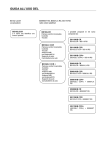
4.2.1.1.2 The collapsed sector
Whereas a collapsed is a gathering of sectors on which a controller is
assigned during a time period of the day. Currently, we consider that a
collapsed sector can only contain elementary sectors.
4.2.1.2
Characteristics of a sector: its ability
A sector noted s, elementary or collapsed, is given a load limit profile as well
as a capacity limit profile: we talk about ability limit profile in general.
4.2.1.2.1 The load limit profile
The load limit profile L(s) corresponds to the graph displaying number of
air-planes that are allowed to be in at the same time. This load limit, noted
L(s,t) can vary during the day, t standing for the time. Indeed, the
different load limits are given as an entry of the problem for each t,
0≤t<24*60. To help expressing the load relaxation, we note L0(s,t) the
state of the profile at the beginning of the solving, that is to say the load limit
profile demanded.
4.2.1.2.2 The capacity limit profile
Analogously, for the load limit profile, the capacity limit profile, noted C(s),
corresponds to the graph displaying the number of air-planes that are
allowed to have entered s during the hour preceding t.
4.2.1.3
The constraint itself
We have just seen that each sector is given an ability limit profile. Besides,
the definition of all the ability limits has been a problem that we encountered
in LCCR, because of a lack of information and LCCR needs coherent
information concerning the load and capacity limits to perform accurate
regulation. But is exactly the constraint expressed ?
4.2.1.3.1 Load constraint
This constraint ensures that, for each sector s, the number of air-planes
present in it at the same time t, can not overpass the load limit L(s,t)of
this sector, only for 0≤t<24*60. We have to give more precision about what
we call “to be present”.
28
4.2.1.3.2 Capacity constraint
Obviously, the constraint concerning the capacity is built in the same spirit.
We give the formal definition afterwards.
4.2.1.3.3 The co-ordination time of a sector: a major feature and impact on ability
To be more precise, we have to introduce the notion of co-ordination time
CT(s)of a given sector s. Each time an air-plane having the flight plan f
enters sector s, we consider in fact that f is present in s CT(s) minute
before its real entrance. In LCCR, the co-ordination time does not vary
during the regulation day.
This co-ordination time plays another role that we have to mention, so as to
be precise: if a flight plan f was scheduled to enter physically a sector s
after t=0, and that, with the co-ordination time CT(s), it is scheduled to
cross it before t=0, LCCR regulates flight plan f only on the part of its
crossing time t such as t≥0. Nevertheless, this happens very rarely and
does not affect regulation in general, since there is almost no regulation at
midnight.
4.2.1.3.3.1 Its impact on load
It is easy to figure out that, the greater the co-ordination time is, the more
constraining the load constraint is. This is why this co-ordination time can be
considered as a major feature of the model when regulation by load.
4.2.1.3.3.2 Its impact on capacity
We note that the co-ordination time CT(s) of sector s does affect the
regulation only in the fact that it shifts the regulated capacity profile to the
left: it does not make the constraint more constraining.
4.2.1.4
Its formal equation
We give the formal equations of the ability constraints, so that there is no
ambiguity left.
4.2.1.4.1 Load
We note NL(s,t) the number of air-planes present (taking into account the
co-ordination time CT(s) of sector s) at time t in sector s, and we note
tor(f,s) the regulated exit time of flight plan f from sector s (o stands for
“out”). Said in a more formal way, this load constraint ensures:
∀s∈S, ∀t∈[0,24*60[,
NL(s,t)={f∈F(s),tir(f,s)CT(s)≤t<tir(f,s)+d(f,s)}≤L(s,t).
4.2.1.4.2 Capacity
There is a major difference between the capacity and the load constraint
usually used. The capacity takes into account all the flight plans that have
been entering a given sector during the last hour, whereas the load
constraint is a more instantaneous measure of sector loading. This notion of
load was introduced to test whether such a constraint could improve the air
traffic regulation, by minimising the global delay of flight plans. LCCR was
partially built to compare a regulation by capacity versus a regulation by
load.
29
So as to make things clear, we also give the capacity constraint formal
equation:
∀s∈S, ∀t∈[0,24*60[,
NC(s,t)={f∈F(s),tir(f,s)-CT(s)≤t<tir(f,s)CT(s)+60}≤C(s,t).
Here, NC(s,t) represents the number of air-planes having entered the
sector s during the full hour preceding t, taking into account the coordination time CT(s) of sector s.
4.2.2
The flight plans equity constraint
This constraint concerns flight plans having the same departure and arrival
aerodromes. If we consider two different flight plans f1 and f2, assuming
that f1 is scheduled to take off before f2. In this case only, the equity
constraint imposes that the initial order of the two flights should not be
inverted after regulation, which means that:
∀f1∈F, ∀f2∈F,
if
da(f1)=da(f2), aa(f1)=aa(f2) and tie(f1)≤tie(f2)
then
tir(f1)≤tir(f2).
This constraint is called an equity constraint because it prevents flight plans
that have a priori identical features, not to be randomly inverted because of
the regulation. LCCR does not express this constraint in this way: an extra
parameter is introduced so as to make the constraint a bit more flexible. This
extra parameter is equity_trigger, expressed in minute, and we
consider the equation:
tir(f1)≤tir(f2)+equity_trigger.
The parameter equity_trigger settable through the solving parameters
panel, allows the two flight plans to be inverted, but not too much and makes
the constraint more operational. In other words, during the solving, f1 is
allowed to take off after f2 only if it does not take off more than
equity_trigger minute after f2.
4.2.3
The flight plans round-trip constraint
This constraint concerns the flight plans that uses the same air-plane to
complete their corresponding journey, i.e. that performs a round-trip journey
described by the two flight plans: it involves that the call sign of the second
leg flight plan is the same as the one leg’s except for the last digit which
must be increased by one, that the aircraft type of the two flight plans is the
same, that the departure aerodrome of each flight plan is the same as the
arrival aerodrome of the other flight. Since these round-trip flights are not
notified in the entry data of LCCR, in order to find these round-trip flight
plans, LCCR uses an additional criteria. A flight plan f2 is the return flight
plan of a flight plan f1, if flight plan f2 is scheduled to depart between
round_trip_mini and round_trip_maxi minute after flight plan f1
scheduled arrival. In equations, it makes: ∀f1∈F, ∀f2∈F,
if
da(f1)=aa(f2), aa(f1)=da(f2), AT(f1)=AT(f2) and
round_trip_mini≤tir(f2)-tor(f1)≤round_trip_maxi
30
then
f1 (the first leg) and f2 (the second leg) is a couple of round-trip flights.
In this case only, the round-trip constraint imposes that the delay of the
return flight plan should be greater or equal to the delay of the one-way
flight:
∀f1∈F, ∀f2∈F, f1 (the first leg) and f2 (the second leg) is a couple of
round-trip flights,
d(f2)+round_trip_trigger≥d(f1).
As for the equity constraint, the parameter round_trip_trigger settable
through the solving parameters panel, allows the constraint to be more
operational and flexible: with it, the delay of the return flight plan f2 is only
impacted if the delay of the one-way flight plan f1 is strictly greater than
round_trip_trigger.
This constraint emphasises the fact that the same air-plane is used for the
two flight plans, and that it needs to be re-prepared after the one-way
journey.
4.2.4
The aerodromes curfew constraint
This constraint concerns the flight plans that take off or land on an
aerodrome a subject to some curfew: during an aerodrome curfew c(a), no
flight can take off nor land on the aerodrome. This implies that the
concerned flight plans can only take off and land respectively outside their
departure and arrival aerodrome curfew. These flight plans will be delayed
or limited in delay so as to respect this constraint.
An exception is accepted when the flight plan was formerly scheduled to
take off or to land respectively during its departure or arrival aerodrome
curfew. Moreover, the curfew on an aerodrome can be made of several
periods. LCCR considers as well curfew on departure as curfew on arrival.
More formally, we can write: ∀f∈F,
if tie(f)∉c(da(f)) then
tir(f)∉c(da(f)) and,
if toe(f)∉c(aa(f)) then
tor(f)∉c(aa(f)).
4.2.5
The category constraint
This constraint handles the flight plans, whose aircraft types have disparate
passenger capacities. This constraint forces flight plans to take into account
the capacity of its passenger welcoming: thus, it introduces the notion of
category.
4.2.5.1
Aircraft categories
LCCR introduces different categories of air-planes, sorted according to the
number of passenger it is able to welcome. Currently, the first category
gathers all aircraft types able to welcome more than 300 passengers, the
second category gathers all aircraft types able to welcome between 100 and
300 passengers…
31
We note CA(at) the category of the aircraft type at. For each category
ca∈CA where CA is the set of all categories, max(ca) (expressed in minute)
is the maximum delay that all the flight plans of that category can accept.
Thus:
∀f∈F, ∃ca∈CA, CA(AT(f))=ca, 0≤d(f)≤max(ca).
4.2.5.2
How it interferes with the priority constraint
Thanks to these categories, LCCR forces the flight plans to accept a
maximum delay according to the category their aircraft belong to. Usually,
the less the category is, the less the maximum delay is. But it is not always
the case, and the end-user can set the categories as she wants.
Nevertheless, in all cases the category i is always considered to have a
greater priority than category i+1. These categories enables LCCR to give
different priorities to flight plans of different importance.
4.2.6
The exempted flight plan constraint
Also, LCCR enables the end-user to specify certain flight plans as
exempted, which means that the delay of these flight plans must be null. If f
is such an exempted flight, it means that max0(d)=max(f)=max1(f)=0 so
that we always have d(f)=0.
This constraint is necessary for certain kind of flight plans such as
transatlantic ones on which no regulation can be made since the CFMU
does not control their departure area. This constraint applies also to
humanitarian flight plans, political flight plans, for instance.
4.3
The solver
This part is the most delicate part of this documentation: the reader will have to
read it with much attention if she wants to be able to understand deeply how
LCCR finds a feasible solution.
4.3.1
Before LCCR enumerates
4.3.1.1
Domain-variables definition
LCCR first defines all the domain-variables coming from the flight plans
(departure times, delay and entry time in each sector, all linked to the delay)
and from the sectors (load or/and capacity limit profile heights). LCCR gives
to these domain-variables their largest domain taking into account their
maximum relaxation. We explain why in the next paragraph.
4.3.1.2
Definition of the constraints
Once the domain-variables are defined, LCCR sets the different constraints,
that is to say, it creates the constraints: the flight plans round-trip
constraints, the flight plans equity-constraints, the aerodromes curfew
constraints, the sectors load constraints (if asked for) and the capacity
constraints (if asked for). At this step, since the domain-variables were given
an initial range corresponding to their maximum relaxation, the problem is
not already constrained as it should be: it is rather constrained with the full
relaxation.
LCCR works this way, in order not to re-built each time the constraints,
which is expensive is computing time: LCCR saves the state of the domainvariables at this level so as to be able to recover it very efficiently.
32
4.3.1.3
Posting the constraints
Now, LCCR is able to post the constraints asked for without relaxation.
LCCR can enter this stage in two different states:
• it is the first time during the current solving that LCCR posts the
constraints and no special method is used;
• it is not the first time that LCCR posts the constraints during the
current solving, and a special method is called, since this step
corresponds to the problem relaxation.
4.3.1.3.1 First time
It is supposed that no relaxation has been performed so far, when entering
this stage. LCCR deals as well with constraints on the ability (load or/and
capacity) profile heights as on the flight plans delays.
4.3.1.3.1.1 The ability limit profile height variable
LCCR posts on each sector the constraint on the height of its ability limit
profile (load or/and capacity): this constraint ensures that the current
demanded ability is not over-passed. However, it is possible that the
constraint on this height is not feasible because the regulation problem is
over-constrained: in this case, LCCR grants the necessary amount of
relaxation (provided this amount does not exceed the maximum relaxation
allowed when defining the domain-variables) so as the constraint posting
does not fail, and thus, so that the satisfaction problem is respected. If, with
all the relaxation allowed, one ability cannot be respected on a given sector,
the corresponding constraint is ignored on that precise sector and LCCR
solver fails to find a feasible solution.
4.3.1.3.1.2 The flight plan delay variable
Then, LCCR posts the constraints on the flight plans delays domainvariable, so as to specify that these variables are not allowed to exceed their
current maximal value. However, it may happen that certain flight plans
delay cannot be curbed enough: for these flight plans, LCCR grants just the
necessary relaxation (provided it does not exceed the maximum relaxation
given when defining the domain-variables) so that these flight plans can be
placed.
In opposition to what is performed for the ability constraint posting, if a flight
plan can not respect its demand maximum delay constraint, LCCR can
always relax its delay within its maximum delay relaxation, so that this stage
is always successful.
4.3.1.3.2 Not the first time: relaxation
In this case, it is not the first time LCCR posts the constraints: it is only the
case when LCCR performs some relaxation. In this case, the two types of
constraints are re-posted in the same order, but with the relevant domainvariables upper bounds re-adjusted.
4.3.1.4
Enumeration
All the constraints are posted, now the enumeration can start. We explain in
the next paragraph the different strategies used in LCCR. However, each
time the enumeration fails (partially or not), and that some relaxation is
asked for, LCCR returns to the step before, that is to say to the constraints
posting.
33
4.3.2
The main line strategy
LCCR tries to place all the given flight plans, respecting the different
constraints. The strategy it adopts depends on the kind of regulation that the
end-user selects: such a strategy that is set throughout the heuristic, will not
be the same if the end-user launches a search for a load regulation as the
one to regulate by capacity. As for the other constraints, the strategy can
change a lot the quality of the results, and we will give some details so as to
understand the importance of the priority parameters attached to the roundtrip and the equity constraints. Nevertheless, we can describe a global
strategy of LCCR.
4.3.2.1
A strategy to detect the flight plans that cannot be placed
This mechanism has been implemented to detect as soon as possible the
flight plans that do not have any feasible delay value. This occurs when the
constraints of the problem are not able to detect an inconsistency. To avoid
that, and before choosing a group of flight plans, LCCR takes all the flight
plans not yet placed one after another.
For each flight plan f of these flight plans, LCCR tries to place it with one of
the value of its domain. If the constraints fail each time, it means that the
flight plan f cannot be placed. Once all these flight plans have been tested,
LCCR keeps only the flight plans that cannot be placed: we know that the
problem will not have any solution if we do not grant to these flight plans an
extra relaxation to their maximum delay. That is the reason why LCCR
relaxes these flight plans with an extra step of relaxation (how this relaxation
proceeds will be explained in the relaxation paragraph).
This process if continued as long as there is no more flight plan that cannot
be placed. If this stage fails, relaxation on the abilities (load or/and capacity)
of the sectors is launched and this stage is given up.
4.3.2.2
A strategy to choose the groups of flight plans
Indeed, LCCR does not try to place all the flight plans at the same time. It
divides the set F into smaller sets, and then tries to place these sets of flight
plans. The way these groups of flight plans are chosen will be explained
further, as well as the order in which they are instantiated within it. Once a
group of flight plans has been totally instantiated (which implies with
success), the flight plans of this group are never re-put into question,
provided the solver is not re-launched. This means that the heuristic is
highly important in this context.
Besides, the number of flight plans taken to build one group of flight plans is
a parameter noted group_percentage that is settable through the solving
parameters panel: LCCR gives the end-user the opportunity to indicate what
percentage of flight plans are to be taken at each group definition. This
percentage is the percentage related to the total number of flight plans to be
regulated. The smaller this percentage group_percentage is, the slower
the solver is to provide a solution. We will discuss more about this
parameter when we have talked about the heuristic.
4.3.2.3
A strategy in the order the flight plans are instantiated within a
group
As explained upper, there is another heuristic defined, which handles the
flight plans of a group. Once a group of flight plans has been chosen by
LCCR, these flight plans are going to be instantiated. This strategy defines
34
in what order the flight plans are placed, and it depends on the options
selected in the solving parameters panel, as we will see.
4.3.2.4
4.3.3
A strategy for the delay of a given flight plan
At an even finer level, LCCR defines a strategy that chooses a feasible
delay value for a given flight plan to be instantiated. This strategy will be
discussed later on, and we will see that it depends on some other solving
parameters dealing with the optimised results query.
Different strategies for different aims
4.3.3.1
The round-trip priority
First note that this option is effective only when the round-trip constraint is
enabled. When this option is selected, LCCR will give priority to the roundtrip flight plans. And yet, it does not mean that LCCR places first the roundtrip flight plans. The strategy adopted is quite different when this option is
enabled. Indeed, when a flight plan is bound to be placed, LCCR looks if this
flight plan is part of a round-trip flight plan: and if it is the case, it does not
only place this flight plan, but also the flight plan linked to it. And to improve
its chance of success, LCCR tries to place first the one-way flight plan (even
if it was not the one selected formerly to be instantiated), and only after it
tries to place the return flight plan if the one-way flight plan could be placed.
This option is most of the time to be selected because it prevents LCCR
from placing the second leg flight plan of a round-trip flight plans couple with
very little delay, whereas its corresponding first leg flight plan has not been
placed yet, imposing then that its delay should be very limited because of
the round-trip constraint (posted formerly on the couple of flight plans). If the
round-trip priority is inactive and that LCCR first places the second leg flight
plan without placing the first leg as well, relaxation on the first leg flight plan
is inefficient since its maximum delay is already majored due to the
placement of its second leg flight plan.
4.3.3.2
The equity priority
As for the round-trip priority, this equity priority is only efficient provided the
equity constraint has been set active. When this option is made active, the
way a solution is searched is similar to the strategy used when the round-trip
priority is activated. Thus, when LCCR tries to place a flight plan, it looks
whether this flight plan belongs to a group of flight plans linked by an equity
constraint. If it is the case, LCCR not only tries to place the selected flight
plan, but also all the equity flight plans estimated to depart before the flight
plan selected. The order these flight plans are taken to be instantiated is
given by their estimated departure time: locally, the first flight plan to take off
is the first to be placed. When one of the equity constrained linked flight plan
cannot be placed, LCCR considers that the former flight plan selected
cannot be placed.
As for the previous priority, it is very wise always to activate this option. The
reason is about the same as for the round-trip priority: if you do not activate
this option, LCCR may place a flight plan with very little delay, while this
flight plan belongs to a group of equity-constrained flight plans and that this
flight plan is estimated to take off one of the last among the group. If the
equity priority is inactive and that LCCR first places this flight plan, the
maximum delay of the other flight plans of the group will be constrained to
be somehow less delayed than the flight plan placed, and relaxation on
them will be useless.
35
4.3.3.3
The round-trip and the equity priorities altogether
When both of the priorities are activated and if both their corresponding
constrains are enabled, LCCR gives priority as well on the round-tripconstrained and the equity-constrained flight plans. In this case, when LCCR
tries to place a flight plan, it first deals with the round-trip case. Afterwards, it
deals with the equity case. Nevertheless, these two options selected
altogether can provide a triggering behaviour to LCCR: if the round-triplinked flight plan is itself part of an equity-constraint, the equity-constraint
flight plans are also considered so as to be placed and so on. The
consequence of this behaviour is that when LCCR tries to place a single
flight plan, it can consequently place a lot of flight plans as well
simultaneously, even if these flight plans are not part of the current flight
plans group.
4.3.3.4
The category priority
This priority is used to decide between two flight plans from the current
selected group that have the same priority of placement. In this precise
case, so as to determine which one is to be placed the first, LCCR looks at
the category their respective aircraft type belongs to, and first tries to place
the one with the smallest category number. In fact, this criterion is very
rarely used because, most of the time, the flight plans have different
priorities of placement.
4.3.3.5
Regulation by load
We now explain the way the regulation by load is performed: thus, we are
going to talk about the heuristic used in LCCR. All what will be discussed
about load is also true concerning the capacity, but we will explain to the
reader later how to make the interpolation.
4.3.3.5.1 Three evaluation tool: the load demand, the load critical and, the load
forecasted profiles
These three profiles are used to build LCCR heuristic: we are going to
describe each one of them, so as to explain part of the heuristic mechanism.
Note that all these profiles are dynamically built: their layout is not constant
within the same solving.
4.3.3.5.1.1 The load demand profile
We now describe one basic measure, which is the load demand profile of a
given sector s, noted LDP(s,t) (or LDP(s) for the profile graph). This
profile is defined for each sector, and it represents the current dynamic load
demand profile; it is defined in the following way.
Considering a sector s, for each flight plan f that crosses s, the load
demand profile is increased by one unit during the interval time ∆t defined
by ∆t={t,tie(f,s)-CT(s)+dmin(f)≤t<toe(f,s)+dmin(f)}. This interval
time represents the current occupation of flight plan f in sector s, as if f
were placed with its current delay lower bound value dmin(f).
When the contribution is defined on sector s for all the crossing flight plans
f∈F(s), we get this load demand profile. This profile’s limit is the load
regulated profile, i.e. when all the crossing flight plans F(s) are placed on
sector s, then the load demand profile is equal to the load regulated profile.
Note that this profile is made of integer values and that it is dynamic.
36
Formally, ∀s∈S, ∀t,
LDP(s,t)=card(f∈S(f),tie(f,s)CT(s)+dmin(f)≤t<tie(f,s)+d(f,s)+dmin(f)).
4.3.3.5.1.2 The load critical profile
To understand how this regulation is done, we have to describe one other
important measure, which is the load critical profile of a given sector s,
noted LCP(s,t) (or LCP(s) for the profile graph).
This profile was designed in order to choose correctly the flight plans the
most urgent to be placed; in other words, this profile helps LCCR to choose
the next sectors to be relaxed if necessary. This profile is defined for each
sector, and it represents the potential difficulty for a sector to accept all the
flight plans scheduled to cross it. More precisely, it is defined in the following
way.
Considering a sector s, for each flight plan f that crosses s, the load critical
profile is increased by one unit during the interval time ∆t defined by
∆t={t,tie(f,s)-CT(s)+dmin(f)≤t<toe(f,s)+dmax(f)}. This interval
time represents the maximum occupation of flight plan f in sector s. Note
that this interval time ∆t is never empty and that it is equal to the demand
and to the regulated crossing interval time of flight plan f in sector s when
flight plan f is placed.
When the contribution is defined on sector s for all the crossing flight plans
f∈F(s), we get this load critical profile. This profile is always above the
load demand profile, and that is why we call it a critical profile. When all the
crossing flight plans F(s) are placed on sector s, then the load critical
profile is equal to the load regulated profile. Note that this profile is made of
integer values and that it is also dynamic.
Formally, ∀s∈S, ∀t,
LCP(s,t)=card(f∈S(f),tie(f,s)-CT(s)+dmin(f)≤t<
tie(f,s)+d(f,s)+dmax(f)).
4.3.3.5.1.3 The load forecasted profile
Another measure allows to refine dynamically the heuristic: this is the load
forecasted profile of a given sector s, noted LFP(s,t) (or LFP(s) for the
profile graph).
This profile was also designed in order to choose correctly the flight plans
the most urgent to be placed. This profile is defined for each sector, and it
represents the potential difficulty for a sector to accept all the flights
scheduled to cross it: this measure is very close to the load critical profile,
but it is less critical however. It is defined in the following way.
Considering a sector s, for each flight plan f which crosses s, the load
forecasted profile is increased by (d(f,s)+CT(s))/(dmax(f)dmin(f)+d(f,s)+CT(s)) unit during the interval time ∆t defined by
∆t={t,tie(f,s)-CT(s)+dmin(f)≤t<toe(f,s)+dmax(f)}. This interval
time represents the maximum occupation of flight plan f in sector s (as for
the critical profile). Note that this interval time ∆t is never empty and that it
is also equal to the demand and regulated crossing interval time of flight
plan f in sector s when flight plan f is placed.
When the contribution is defined on sector s for all the crossing flight plans
f∈F(s), we get this load forecasted profile. This profile is a normalisation of
37
the current load critical profile, representing an equi-probabilistic load profile,
and that is why we call it a forecasted profile. When all the crossing flight
plans F(s) are placed on sector s, then the load forecasted profile is equal
to the load regulated profile. Note that this profile is made of real floating
values and that it is once again dynamic.
Formally, ∀s∈S, ∀t,
LFP(s,t)=
d(f,s)+ CT(s)
L(s,t)
f∈S(f) d max(f)- d min(f)+ d(f,s)+ CT(s)
∑
where:
δL(s,t)=1 if tie(f,s)-CT(s)+dmin(f)≤t<tie(f,s)+d(f,s)+dmax(f),
δL(s,t)=0 otherwise.
4.3.3.5.2 Link with the load profiles : the load over volumes
All these profiles enable LCCR to consider some other functions helpful for
the heuristic, mostly during the relaxation. Note that all these functions take
into account the co-ordination time CT(s) of each sector s, which magnifies
a lot the load constraint.
4.3.3.5.2.1 The load demand over volume
For a given sector, the load demand profile is considered so as to be
compared with the load limit profile, which is the graph representing at any
time t the load limit accepted by the corresponding sector, and that was
already noted L(s,t) for a given sector s (or L(s) for the profile graph).
By comparing these load demand over volumes, LCCR sorts the sectors.
The dynamic upper surface (which is called a volume) between the load limit
profile and the load demand profile is called the load demand over volume,
and is notes LDOV(s) for a given sector s.
Formally, ∀s∈S,
t =24*60−1
LDOV(s)=
∑ max(LDP(s,t)− L(s,t),0).
t =0
We also define the load demand volume LDV(s), which is the total amount
of minute during which the sector s is crossed (including the co-ordination
time CT(s)):
t =24*60−1
LDV(s)=
∑ LDP(s,t).
t =0
Note that this measure is constant all solving long: what LCCR performs is
to shift this load volume so as not to overpass the load limit profile.
4.3.3.5.2.2 The load critical over volume
For a given sector, the load critical profile is also evaluated so as to be
compared to the load limit profile. When the load critical profile does never
exceeds the load limit profile, LCCR is ensured that there will no problem on
the given sector, from a load constraint point of view at least. Nevertheless,
when this load critical profile exceeds the load limit profile, it is possible that
the corresponding sector might be overloaded. Off course, this does not
mean that it will be overloaded and that regulation has to be performed on it,
but by comparing these load critical over volumes, LCCR can sort the
sectors.
The dynamic upper surface (which is called a volume) between the load limit
profile and the load critical profile is called the load critical over volume, and
is noted LCOV(s) for a given sector s.
38
Formally, ∀s∈S,
t =24*60−1
LCOV(s)=
∑ max(LCP(s,t)− L(s,t),0).
t =0
We also define the load critical volume LCV(s), which is the total amount of
minute during which the sector s would be crossed (including the coordination time CT(s)) if each flight plan f∈F(s) of all the flight plans
crossing it crossed it during a period increased by its delay domain-variable
d(f) range dmax(f)-dmin(f):
t =24*60−1
LCV(s)=
∑ LCP(s,t).
t =0
Here, this measure is not constant but tends to be equal to the load demand
volume LDV(s): the more flight plans are placed, the closer the load critical
volume to the load demand volume is. This value does not represent
anything concrete, that is why, afterwards, we will consider a value deduced
from it.
4.3.3.5.2.3 The load forecasted over volume
For a given sector, the load forecasted profile is evaluated so as to be
compared to the load limit profile. By comparing these load forecasted over
volumes, LCCR can sort the sectors.
The dynamic upper surface (which is called a volume) between the load limit
profile and the load forecasted profile is called the load forecasted over
volume, and is noted LFOV(s) for a given sector s.
Formally, ∀s∈S,
t = 24*60 − 1
LFOV(s)=
∑ max(LFP(s,t)− L(s,t),0).
t =0
We do not have to introduce the load forecasted volume LFV(s), since it is
equal to the constant load demand volume LDV(s):
LFV(s)=LDV(s).
4.3.3.5.3 The heuristic to choose a group of flight plans
Now, we return to the heuristic used to select a group of flight plans. When
LCCR regulates by load, it uses fully these load profiles.
LCCR computes the load profiles on all the sectors (elementary and
collapsed). For each one of these profiles, it defines the load over volumes,
which represent the surfaces of the load profiles above the load limit profile,
as we just introduced it. LCCR does not try to place all the flight plans of a
sector, but instead, it tries to place first the most critical flight plans. To do
so, LCCR considers a load priority function for each flight plan f, which will
be referred to by the notation pL(f).
4.3.3.5.3.1 The flight plan load priority function
We now give the way the flight plan load priority function is built. Given a
flight plan f, we consider recursively all the sectors (elementary and
collapsed) that it might physically cross, S(f). And, for each sector s∈S(f)
it crosses, LCCR computes its contribution to the eventual overloading
volume during the interval time it would cross s if its delay d(f) were equal
to its current delay lower bound value dmin(f). This contribution is added to
pL(f), which was previously reset to 0.
More formerly,
39
∀f∈F,
pL(f)=
∑
t =t ie(f,s)-CT(s)+ d(f,s)+ d min(f)-1
s∈S(f)
∑ max(LDP(s,t)− L(s,t),0).
t =t ie(f,s)-CT(s)+ d min(f)
4.3.3.5.3.2 How the flight plans are ordered
Thus, we get for each flight plan a sum of all the crossed sectors
contribution. LCCR sorts the flight plans not yet placed by decreasing
priority. It then normalises the load priority by giving the value 100 to the
flight plan with the highest load priority noted PL=max{pL(f),f∈F}, and for
each flight plan f, the previous priority pL(f) is replaced by pL(f)/PL.
Now the flight plans are sorted and LCCR chooses the next group of flight
plans to be placed. The size of this group depends on a solving parameter,
which is the flight plan group percentage noted group_percentage
(expressed between 0 and 1). This parameter represents the percentage of
the total flight plans to be chosen each time for one group. Only
card(F)*group_percentage flight plans will be chosen, except if all the
flight plans not yet placed have a null priority: in this case, all the flight plans
left are selected. Note that this special case appears when all the flight plans
not yet placed can be placed at their current delay lower bound, since their
priority is null.
4.3.3.5.4 The heuristic to choose a flight inside a group
This heuristic is half dynamic, depending on a quality factor referred as
search_quality (ranging from 0 to 999) set through the solving
parameters panel. Indeed, each time 1000-search_quality flight plans
are placed, LCCR re-computes the order in which it chooses the flight plans
not yet placed inside the same current group. The order is given by the
decreasing load priority for each flight plan, computed in the previous stage.
Thus, the higher this search quality factor is, the finer and the more dynamic
the heuristic is.
4.3.3.5.5 The heuristic to choose a delay for a given flight plan
4.3.3.5.5.1 No optimisation asked for
This heuristic is very basic when the optimisation is not set on the solving
parameters panel. When LCCR tries to place a flight plan f, it simply tries to
place it with a delay equal to the lower bound value dmin(f) of its current
delay domain-variable d(f). This strategy globally tends to minimise the
total sum of the flight plans delays.
4.3.3.5.5.2 Optimisation parameters
However, the strategy is more complex when some optimisation parameters
are active. Three optimisation options are available in LCCR: either the enduser chooses to minimise the number of flight plans delayed, or she wants
to minimise the total delay sum of all the flight plans (said in another way,
the average delay per flight plan), or she decides to minimise the average
delay per delayed flight plan (average delay per delayed movement).
4.3.3.5.5.2.1 Number of flight plans delayed optimisation
Before setting a given flight plan f to a feasible delay value, LCCR tries a
range of feasible delay value. LCCR contemplates each of these feasible
40
delay values, and will try to instantiate the delay domain-variable d(f) to
the value that minimises the number of flight plans delayed.
The way to know what is the best value is to store the state of all the
domain-variables, instantiate the corresponding flight plan delay domainvariable d(f) to one of its domain value, look at the constraints propagation
deduction, and keep the value that minimises our criteria.
4.3.3.5.5.2.2 Average delay per flight plan optimisation
Before setting a given flight plan f to a feasible delay value, LCCR tries a
range of feasible delay value. LCCR contemplates each of these feasible
delay values, and will try to instantiate the delay domain-variable d(f) to
the value that minimises the total sum of the flight plans delays.
The way to know what is the best value is to store the state of all the
domain-variables, instantiate the corresponding flight plan delay domainvariable d(f) to one of its domain value, look at the constraints propagation
deduction, and keep the value that minimises our criteria.
4.3.3.5.5.2.3 Average delay per delayed flight plan optimisation
The technique is about the same. Before setting a given flight plan f to a
feasible delay value, LCCR tries a range of feasible delay values. LCCR
contemplates each of these feasible delay values, and will try to instantiate
the delay domain-variable d(f) to the value that minimises the average
delay per delayed flight plan.
4.3.3.6
Regulation by capacity
There is not much to say concerning the regulation by capacity: everything
that has been said concerning the load regulation can be interpreted as well
for the capacity, just by considering a crossing time duration of 60 minutes
for each sector crossed by a flight plan.
4.3.3.6.1 Link with the load
In other words, LCCR works with capacity in the same way as for the load;
all the equations remain correct if you replace d(f,s)+CT(s) by the value
60.
4.3.3.6.2 The formal equations
So as the reader makes no confusion, we give the definitions related to the
capacity regulation:
∀s∈S, ∀t,
CDP(s,t)=card(f∈S(f),tie(f,s)-CT(s)+dmin(f)≤t<tie(f,s)CT(s)+60+dmin(f)),
CCP(s,t)=card(f∈S(f),tie(f,s)-CT(s)+dmin(f)≤t< tie(f,s)CT(s)+60+dmax(f)),
CFP(s,t)=
where:
δC(s,t)=1
if
CT(s)+60+dmax(f)),
60
C(s,t)
f∈S(f) d max(f)- d min(f)+ 60
∑
tie(f,s)-CT(s)+dmin(f)≤t<tie(f,s)-
41
δC(s,t)=0 otherwise
t = 24*60 − 1
CDOV(s)=
∑ max(CDP(s,t)− C(s,t),0)
t =0
t = 24*60 − 1
CCOV(s)=
∑ max(CCP(s,t)− C(s,t),0)
t =0
t =24*60−1
CFOV(s)=
∑ max(CFP(s,t)− C(s,t),0).
t =0
∀f∈F,
pC(f)=
∑
t =tie(f,s)-CT(s)+60 + d min(f)-1
s∈S(f)
∑ max(CDP(s,t)− C(s,t),0).
t =t ie(f,s)-CT(s)+ d min(f)
4.3.3.6.3 Same mechanism
The operations described concerning the load regulation are the same for
the capacity regulation: the different steps do not change, only the flight plan
priority and the profiles functions change.
4.3.3.7
Regulation by load and capacity
Regulation by load and by capacity is possible as well on LCCR.
Nevertheless, because of memory use restrictions, it is not advisable to
launch a solving on an important set of data exceeding 20 000 flight plans.
LCCR considers as well the load priority of a given flight plan f, as its
capacity priority: the priority of the flight plan f is p(f)= pL(f)+pC(f). With
this extra datum, LCCR follows the same steps as described before. Nothing
more special is to be noted concerning this double regulation, except for the
relaxation, and we will discuss this issue later.
4.3.4
Relaxation
This mechanism is essential in LCCR, since most of the data are overconstrained. LCCR provides the opportunity to soften somehow different
constraints of the problem. Without relaxation, no solution could be
provided, simply because there is no solution. That is the reason why we
stress the importance of the corresponding solving parameters, which
modify a lot the physiognomy of a solution. Much care is to be brought by
the end-user on the definition of the different relaxation parameters.
4.3.4.1
Global mechanism
There is a global mechanism concerning the relaxation on LCCR: LCCR
always relaxes first on the maximum delay of the flight plans, and if there is
still no solution, it relaxes the abilities of the sectors (load or/and capacity).
We first detail the mechanism concerning the flight plans delay maximum
relaxation, and then the relaxation on the sectors abilities.
4.3.4.2
The flight plans delay relaxation
This is the first kind of relaxation performed by LCCR. This relaxation occurs
when a group of flight plans cannot be placed entirely, that is to say when
LCCR does not find any proper delay value for at least one flight plan. This
42
relaxation is active only if the corresponding solving parameter is enabled
(by default, it is), and if the other related parameters
(delay_relaxation_step_percentage
and
delay_relaxation_maximum_percentage) values are coherent.
In this case, LCCR gives some extra relaxation by one step of relaxation to
all the flight plans not yet placed. This step is a customisable parameter of
the
solving
parameters
panel,
and
we
note
it
delay_relaxation_step_percentage. Let us explain how this
relaxation is performed on a flight plan f not yet placed.
• If flight plan f has already used the maximum allowed relaxation, that
is to say if the delay relaxation percentage of flight plan f, noted
relaxation(f),
is
greater
or
equal
to
delay_relaxation_maximum_percentage,
no
additional
relaxation is performed on f.
• Otherwise, flight plan f is increased its delay relaxation percentage by
increasing
relaxation(f)
by
delay_relaxation_step_percentage %, without exceeding
delay_relaxation_maximum_percentage %.
This delay relaxation percentage relaxation(f) is used to define a new
flight plan delay upper bound by replacing its former value by the
corresponding percentage of the initial upper bound delay. More formally, if
flight plan f is performed one relaxation step on its delay domain-variable,
we
can
write
that
relaxation(f)
becomes
min(relaxation(f)+delay_relaxation_step_percentage,delay
_relaxation_maximum_percentage)
and
max(d)
becomes
max0(d)*(1+relaxation(f)), all the percentages being expressed
between 0 and 1. This mechanism ensures that relaxation never overpasses
the global delay_relaxation_maximum_percentage value for all the
flight plans. Moreover, we see that relaxation is inefficient concerning the
exempted flight plans since, for them, max0(d)=0.
Note that, with relaxation, the other constraints (round-trip and equity) are
still handled by the solver.
If no more delay relaxation is possible, i.e. when all the flight plans not yet
placed are already fully relaxed or when delay relaxation is not active, LCCR
performs relaxation on the sectors abilities.
4.3.4.3
The sectors load relaxation
We suppose that the end-user regulates by load and that she has set the
flight maximum delay relaxation mechanism on. This is the second type of
relaxation performed by LCCR. The mechanism described bellow is active
only if the end-user has made the corresponding solving parameters active
and if she has properly defined the other related parameters
(load_relaxation_percentage
and
load_relaxation_maximum_percentage). This relaxation is part of the
sectors abilities relaxation.
When no more flight plan delay relaxation can be performed, LCCR relaxes
the load maximum profile L(s) of some sectors (collapsed and elementary)
so as to provide a solution to the problem. All the problem consists in finding
the relevant sectors to be relaxed, that is to say the sectors that prevent
currently the solver from finding a solution. To find them, LCCR uses all the
previously described evaluation tools.
43
4.3.4.3.1 The sector load priority function
This function is very decisive concerning the quality of the solution when the
problem is over constrained. For a given sector s, we note pL(s) its load
priority concerning the relaxation: this load priority should emphasise the
urgency to relax the corresponding sector in case of load-relaxation. The
more the dynamic load demand profile exceeds the load maximum profile,
the more probable is the sector to be relaxed. This is the idea used when
load relaxation is performed by LCCR. In a empirical manner, we define the
load priority pL(s) of a sector s as a linear combination of its load over
volumes, i.e. of its load demand, critical (normalised as we will see) and
forecasted volumes. More formerly, ∀s∈S,
pL(s)=α*LDOV(s)+β*LFOV(s)+γ*LCOV*(s)
*
with LCOV (s)=LCOV(s)*LDV(s)/LCV(s) with γ≤β≤α.
And so as to give precedence to the load demand over volume which is the
most reliable function, α is greater than β and γ. Moreover, as the load
forecasted volume seems to be empirically better than the load critical
profile, β is greater than γ. The normalised load critical over volume LCOV* is
used instead of the load critical over volume LCOV so as to curb its impact
and so as to get an homogeneous priority expressed in minute. Note that
when LCOV(s) is null, all the other over volumes are null as well and that
consequently pL(s) is also null.
These factors are delicate to tune, and with α=3, β=2 and γ=1, LCCR seems
to be set correctly.
4.3.4.3.2 Selecting the relevant sectors to relax
Once the load priority functions computed for each sector, LCCR sorts the
sectors in a decreasing priority order. It considers the sector s with the
greatest pL(s) noted PL(s) and all the sectors with a priority greater or
equal than PL(s) decreased by ability_relaxation_percentage %
(ability_relaxation_percentage=30 seems to be a well tuned
value): only these selected sectors will be load-relaxed by a additional step
of load_relaxation_step_percentage %. More precisely, the way
each sector s of these sectors is relaxed follows about the same rule as for
the flight plans delay relaxation.
• If the sector s has already used the maximum allowed relaxation, that
is to say if the load relaxation percentage of sector s, noted
is
greater
or
equal
to
relaxationL(s),
load_relaxation_maximum_percentage,
no
additional
relaxation is performed on s.
• Otherwise, sector s is increased its load relaxation percentage by
increasing
relaxationL(s)
by
load_relaxation_step_percentage % without exceeding
load_relaxation_maximum_percentage %.
This load relaxation percentage relaxationL(s) is used to define a new
sector limit profile by raising its former value by the corresponding
percentage of the initial limit profile. More formally, if sector s is performed
one
more
relaxation
step,
its
relaxationL(s)
becomes
min(relaxationL
(s)+load_relaxation_step_percentage,load_relaxation_maxi
mum_percentage) and its limit profile L(s) is raised to L0(s)*(1+
relaxationL(s)) unit (L0(s) being the demand limit profile graph), all the
percentages being expressed between 0 and 1.
44
This mechanism ensures that relaxation never overpasses the global
load_relaxation_maximum_percentage value for all the sectors.
It is important to note that the relaxation is spread all over the day on which
LCCR regulates: indeed, the load limit profile is increased by the same
amount of unit during all day, that is to say with t∈[0,24*60[. As far, an
independent relaxation on each open period is not implemented, but it can
be contemplated.
4.3.4.3.3 No more possible load relaxation
As for the flight plans delay relaxation, when all the sectors have been fully
relaxed, and yet LCCR cannot find a solution to the problem, the solving is
stopped and the end-user is notified that there is no feasible solution.
4.3.4.4
The sectors capacity relaxation
The mechanism is the same as for the load relaxation: the capacity
relaxation has its own capacity_relaxation_step_percentage %,
capacity_relaxation_maximum_percentage %, solving parameters
accessible from the solving parameters panel as well. The capacity priority
function pC(s) is defined in an analogue way, and the capacity relaxation
percentage relaxationC(s) is also defined for each sector s.
4.3.4.5
The sectors load and capacity relaxation
In this case, the mechanism is the same as before, including the solving
stop condition. When both load and capacity regulations are asked for and
that LCCR comes to the ability relaxation, it considers a priority function
p(s) including load and capacity. This priority functions emphasises the
need for a given sector s to be relaxed on load and on capacity: very simply,
it is the sum of the load priority function pL(s) and of the capacity priority
function pC(s), that is to say: ∀s∈S,
p(s)=pL(s)+pF(s).
This priority function is used to sort the sectors in a decreasing order, so that
LCCR only relaxes the most urgent sectors. Note that relaxation on load
cannot be separated from relaxation on capacity, and inversely: each time a
load-relaxation step is performed on a sector, a capacity-relaxation is
performed as well.
5
The code
Now that the model has been presented, we can present the way it was coded.
LCCR was fully coded in C++ for more convenience.
5.1
A word concerning the UNIX to NT migration
To explain why LCCR now runs on a PC, we have to explain its genesis. LCCR
was formerly being developed under HP UNIX V10.2 server wotan, whose
capacities were too weak; however, we did not want to re-write the whole
graphical stuff. That is the reason why we decided to migrate the application to
Microsoft WINDOWS NT V4.0. As a consequence, the prototype can run as
well on HP UNIX as on WINDOWS NT, even if no test has been done so far on
HP UNIX.
5.2
The environment
We here give some details concerning the environment in which LCCR
prototype was coded.
45
5.2.1
Different software libraries used
LCCR uses four main software libraries described bellow:
• Chip-C++ V5.2.1 library, which delivers all the CP kernel enabling to
express variables, constraints, so as to be able to enumerate a
solution. This library is the property of Cosytec SA..
• Loox++ and Loox Extension Pack in C++ V3.3 libraries (LxPack++),
which enable to design the Graphic User Interface (GUI), include
editable lists and Gantt diagrams. These libraries are the property of
Loox Informatique SA..
• X Development Kit V6.1 (XDK) libraries, which enable to emulate a
PC into a X client-server platform. These libraries were useful and
enabled us not to re-code the whole GUI when we came from UNIX to
WINDOWS NT. These libraries are the property of Hummingbird
company.
• At last, X-Designer software that enabled us to design the frames
architecture graphically. This product generates automatically C++
code, which was used in LCCR to handle the graphic, designed via
LxPack++. The product belongs to Imperial Software Technology
(IST) company.
5.2.2
The exact content
We give hereby the exact content of all these libraries, so as re-compilation
and re-linkage of LCCR should be easy with these modules. The reference
are given on PC KAYAK XAs mei.
product
static library path
Chip-C++
%CHIPCDIR%\Lib
LxPac C:\Loox V3.3\Lib
k++
XDK
C:\Program
Files\Exceed
V6.1\xdk\lib
static libraries
chipccrmt.lib
Loox.lib,
Loox++.lib,
LxChart++.lib,
LxPack.lib
xlib.lib,
xmStatXt.lib,
xmstatic.lib,
xlibcon.lib
dynamic libraries
Loox++.dll,
Loox.dll
Xlib.dll…
header files path
%CHIPCDIR%\Include
C:\Loox V3.3\Include
C:\Program
Files\Exceed
V6.1\xdk\include
5.2.3
To recompile: the mode of compilation and of linkage
It is essential to know the way the application was compiled and linked so as
to be able to rebuilt it after some code modification.
The application was developed under Microsoft Developer Studio V6.0
Rapid Application Development (RAD). This RAD proposes a multithreaded
dynamic linkage, which was used. This mode must be re-used to re-compile
LCCR. No other major feature is to be specific for its re-compilation and relinkage.
5.2.4
At run-time
Some of these libraries are still necessary in order to execute LCCR. This is
the case of the LxPack++ and of the XDK dynamical linked libraries, for
instance.
5.3
The application architecture
We will not describe precisely how LCCR was coded, but we give the main
lines adopted, that is to say the LCCR architecture.
46
5.3.1
General architecture
We can describe LCCR objects in a global way: LCCR uses aerodrome,
sector, aircraft type, category, flight classes. LCCR also introduce the notion
of ability class that describes aerodrome and sector capacity or/and load
limit profile and open periods. LCCR also manipulates collections of
instances of those classes.
The code is commented as much as possible (even if a code is never
commented enough) so as to enable the developer to understand the
purpose of classes, functions and methods. We do hope the names given to
these objects are evocative enough.
5.3.2
The COFEE data extraction
The extraction of COFEE environment data is performed by LCCR, so as to
provide the necessary LCCR files: these LCCR files constitute the entry data
of the application. The COFEE data are not directly taken as entry data, but
are beforehand read and put into a LCCR format to provide a steady entry
point for LCCR.
The reason for the creation of intermediate files is that the COFEE files
architecture does not fit in the way LCCR treats the data, and without the
creation of the LCCR intermediate files, the reading of the entry data would
be too long each time.
5.3.2.1
Necessity of an intervention by hand
However, LCCR needs the COFEE extraction already submitted and the
COFEE data locally in the proper directory gathered. LCCR does not call
COFEE and tell it to submit the necessary queries, retrieve the data from the
queries result: it is the responsibility of the end-user to do that job, and to put
the information retrieved by COFEE in a proper directory.
5.3.2.2
The flight plans file
From COFEE is only taken the environment for the day on which the enduser wishes to make some regulation simulation. When LCCR prototype
was started, the information concerning the flight plans was not correctly
available through COFEE. That is the reason why we use an heterogeneous
source of data concerning the fight plans description: the flight plans entry
data come from the all-flights file, which describes all the flight plans for a
given day. This file should be present as well, so that LCCR data extraction
should be possible.
5.3.2.3
The permanent LCCR files
In addition, LCCR, uses some permanent LCCR files, which should not be
touched by the end-user. These files give the information concerning the
different categories, the default capacities of sectors. Without them, LCCR
will not be able to read any LCCR data.
5.3.2.4
The impact on the object architecture
LCCR code includes some data extraction classes, which are specific to that
task and derived from the base classes introduced upper.
5.3.3
The LCCR data reading
This operation enables to load the entry LCCR data into memory. The
objects created are instances of constraints classes derived from the base
47
classes already introduced. Notably, these classes use the CHIP domainvariables and constraints.
5.3.4
The LCCR solver
The solver uses the previous objects and defines correctly the domainvariables and the constraints posted on them. Its aim is to built a search
tree, so as to find a solution.
5.3.5
The LCCR GUI
The GUI interface is made mainly of editable lists and chart diagrams. LCCR
uses instances of classes representing each of these objects to represent
them, and to interact with them.
6
Index
We sum up some notations used throughout this document, so as to make its
reading easier.
aa(f)
arrival aerodrome of flight plan f
AT(f)
aircraft type of flight plan f
CA(at)
category of the aircraft type at
max(ca)
maximum delay of category ca
CT(s)
co-ordination time of sector s
da(f)
departure aerodrome of flight plan f
c(a)
curfew of aerodrome a (set of times)
C(s)
capacity limit profile graph of sector s
C0(s)
capacity limit initial profile graph of sector s (demand)
C(s,t)
capacity limit profile of sector s at time t
C0(s,t)
capacity limit initial profile of sector s at time t (demand)
CCOV(s)
capacity critical over volume of sector s
CCP(s,t)
capacity critical profile of sector s at time t
CDOV(s)
capacity demand over volume of sector s
CDP(s,t)
capacity demand profile of sector s at time t
CFOV(s)
capacity forecasted over volume of sector s
CFP(s,t)
capacity forecasted profile of sector s at time t
d(f)
delay of flight plan f (domain-variable)
F(s)
set of flight plans crossing sector s (elementary or collapsed)
dmax(f)
flight plan f delay d(f) upper-bound
dmin(f)
flight plan f delay d(f) lower-bound
d(f,s)
physical crossing duration of flight plan f in sector s (not
taking into account the sector co-ordination time CT(s))
L(s)
load limit profile graph of sector s
L0(s)
load limit initial profile graph of sector s (demand)
L(s,t)
load limit profile of sector s at time t
L0(s,t)
load limit initial profile of sector s at time t (demand)
48
LCOV(s)
load critical over volume of sector s
LCP(s,t)
load critical profile of sector s at time t
LDOV(s)
load demand over volume of sector s
LDP(s,t)
load demand profile of sector s at time t
LFOV(s)
load forecasted over volume of sector s
LFP(s,t)
load forecasted profile of sector s at time t
max(f)
current maximum value of dmax(f)
max0(f)
initial maximum value of max(f) (without any relaxation)
max1(f)
final maximum value of max(f) (with relaxation)
NC(s,t)
number of flight plans having entered sector s during the
hour preceding time t (taking into account the sector coordination time CT(s))
NL(s,t)
number of flight plans present in sector s at time t (taking
into account the sector co-ordination time CT(s))
p(f)
priority function of flight plan f
p(s)
relaxation priority function of sector s
pC(f)
capacity priority function of flight plan f
pC(s)
capacity relaxation priority function of sector s
pL(f)
load priority function of flight plan f
pL(s)
load relaxation priority function of sector s
relaxation(f)
delay relaxation percentage of flight plan f
relaxationC(s)
capacity relaxation percentage of sector s
relaxationL(s)
load relaxation percentage of sector s
S(f)
set of sectors (elementary and collapsed) crossed by flight
plan f
ti(f)
i
departure time of flight plan f
t e(f)
estimated departure time of flight plan f
tir(f)
regulated departure time of flight plan f
i
t (f,s)
entry time of flight plan f in sector s
tie(f,s)
estimated entry time of flight plan f in sector s
i
t r(f,s)
regulated entry time of flight plan f in sector s
to(f)
arrival time of flight plan f
o
t e(f)
estimated arrival time of flight plan f
tor(f)
regulated arrival time of flight plan f
o
t (f,s)
exit time of flight plan f from sector s
toe(f,s)
estimated exit time of flight plan f from sector s
o
t r(f,s)
regulated exit time of flight plan f from sector s
49
50
PART THREE
LCCR
USER’S MANUAL
51
1
Introduction
1.1
Acknowledgement
This document concerns the end-user of the LCCR prototype. This document is a
user one and it describes LCCR operational facilities: it is aimed at giving the
necessary information concerning the way the prototype is to be used. The person
who wishes to get technical documentation is prompted to refer to the LCCR
reference manual.
1.2
The problematic: reminder
Let us give a short reminder of the context in which LCCR prototype was elaborated.
Besides, we will refer to the LCCR prototype by naming it LCCR, so as to make
things easier from now on.
The CFMU is given the responsibility to regulate the taking-off of air-planes (we talk
more commonly of flight plans) from Europe, so that the different physical sectors
and aerodromes should not be overloaded. This charge is done in real time by the air
traffic controllers in Brussels. Here, to regulate an air-plane means to delay its
departure time, if necessary. The constraint of load and capacity are not the only
ones, and there are other constraints such as equity constraints (concerning flight
plans with same departure and same destination), and priorities constraints
(concerning flight plans of air-planes presenting different passengers capacity).
2
What LCCR proposes
So far, this regulation mission is given to the CASA system, which works with slots
allocation. LCCR proposes to make up this regulation, regarding the main target,
which is to regulate all the flight plans over all the sectors. This regulation is
obviously a simulation.
2.1
What LCCR is not
LCCR is absolutely not a real-time application, since it was not designed for.
The data concerning the flight plans are given as an entry to LCCR;
nevertheless, the data resulting from the regulation made by LCCR is never
given back to the system that provided the entry data. However, this does not
imply that it would not be feasible with the technology used in LCCR…
2.2
LCCR purpose
LCCR purpose is to provide a decision help application for the CFMU
controllers: thus, for a given day and all the flight plans scheduled during that
day by the air companies, LCCR proposes a regulation simulation all over
Europe, restrictively on the flight plans scheduled to be departed on that given
day. This regulation is limited to the sectors, even if the aerodromes curfew
constraint is taken into account; no regulation is performed on the aerodromes
otherwise. To be a decision help application, on the one side it presents the
demand as well on charts and on lists, on the other side, it presents the result
of regulation. A particular effort was brought concerning the different tools of
monitoring, so as to enable the end-user (an air traffic controller) to determine
quickly what flight plan or what sector is mostly responsible for a given delay.
3
The user and the environment
We describe in this section the conditions and the resources required, so that the
LCCR prototype can run properly.
52
3.1
The user
LCCR is a single user application: no particular thing is to be said about that.
There is no particular profile per end-user, so that every potential end-user
shares the same environment. Note that the parameters (different from the
data) modified inside LCCR are saved in preferences files.
Moreover, LCCR is a single document application, which means that it can only
handle one set of data at the same time: this set of demand data represents the
entry data of the regulation problem for a given date DD.MM.YYYY.
3.2
The application global environment
Some special attention is to be brought on a environment variable that should
be set correctly before starting LCCR. This variable’s name is LCCRPATH and
it should point to the directory where the COFEE environment data
(environment is to be thought in terms of regulation) extracted lie. We call this
directory the LCCR path, and in the future, every directory will be referred
relatively to that root path.
In wrong cases, LCCR issues two kinds of error message boxes:
LCCRPATH environment variable not set
LCCRPATH environment variable badly set
3.2.1
Possible confusion on the word extraction
So that the reader makes no confusion, we should warn her that we often
use the same word for two different things. Indeed, when we talk about
extraction, it can refer either to COFEE data environment extraction via the
software COFEE, or to the extraction available in the LCCR prototype to
translate the COFEE data environment and the ALL_FLIGHTS data flight
plans into the LCCR entry demand data. In the future, we talk of COFEE
extraction in the first case, and of LCCR extraction in the second case.
3.2.2
The permanent data files
LCCR uses two types of demand data files as an entry for the loading. Once
some LCCR extraction has been completed, the end-user can load the
LCCR demand data produced by this extraction. However, LCCR needs the
53
following files placed in directory LCCR_ALWAYS, so as to complete
properly the LCCR extraction, as well as the data loading:
• aerodromes_default_capacities.lccr,
collapsed_sectors_default_capacities.lccr and
elementary_sectors_default_capacities.lccr for the LCCR
extraction; these files are used when the extracted COFEE files do
not provide any capacity for the corresponding item;
• categories.lccr for the loading.
3.2.3
The COFEE environment data files
These files should be present it the directory named JYYYYMMDD, which
gathers the extracted COFEE data of the environment corresponding to the
date DD.MM.YYYY (for instance, J19990702 for the day 02.07.1999). The
exhaustive list of the files is:
•
ACTP.sst, ACTPIDEN.sst for the aircraft types;
•
AD.sst, ADTINFO.sst, ADUA.sst for the aerodromes;
•
CF.sst, CFAT.sst, CFCLSC.sst, CFELSC.sst, CFFCPR.sst for
the configurations;
•
CLSC.sst, CLSCAS.sst, CLSCCF.sst for the collapsed sectors;
•
CP.sst, CPPE.sst, CPTA.sst, CPTE.sst for the capacities;
•
ELSC.sst, ELSCCF.sst for the elementary sectors.
Note that these files are provided thanks to the COFEE software, which
should be normally installed on the same machine as the LCCR prototype.
COFEE produces these data environment files, through the COFEE data
environment extraction module.
3.2.4
3.2.5
The ALL_FLIGHTS flights data file
Moreover, LCCR needs the flight plans description file, which is commonly
called the ALL_FLIGHTS data file. For date DD.MM.YYYY, this file should
also be present in the directory named JYYYYMMDD, and its name should
be FLIGHTS.sst.
The LCCR files
3.2.5.1
The basic demand
The LCCR demand data files are produced by LCCR extraction operation,
and for an extraction of the date DD.MM.YYYY, the following LCCR files are
created
in
the
(newly
created
if
necessary)
directory
DEMAND_19000101_000000 standing in directory LCCRYYYYMMDD (also
created if necessary):
• aerodromes.lccr for the aerodromes;
• aircraft_types.lccr for the aircraft types;
• collapsed_sectors.lccr for the collapsed sectors;
• elementary_sectors.lccr for the elementary sectors;
• flights.lccr for the flight plans.
3.2.5.2
Other possible demands
LCCR enables the end-user to save the current solution set (data present in
memory)
into
another
demand
directory
named
DEMAND_yyyymmdd_hhmmss (created in directory LCCRYYYYMMDD
corresponding to date DD.MM.YYYY) where dd.mm.yyyy is the date when
the data are saved, hh:mm:ss the corresponding time.
54
4
The Graphic User Interface
The Graphic User Interface (GUI) is the main frame of the application. We first
describe the overall layout, then the different menus, the editable lists and the
diagram charts.
4.1
Overall layout
The application is composed by a main window with menus, and a splitter,
which divides the main window into two dependently resizable frames (the
upper frame and the lower frame). Moreover, there are three special text fields
to give some relevant information about the state of the application: the
environment field, the status field, the message field.
Some message boxes are displayed to allow the end-user to confirm actions,
abort actions, enter some needed value…
LCCR GUI overall layout
4.2
The menus
The menus allow the end-user to perform some actions described bellow.
However, we notify the reader that some actions can also be triggered through
the keyboard (by shortcut or by accelerator key). For instance, the function
<File.Open> can be triggered in three manners:
• either the end-user presses the <File> menu, and then presses the
<Open> function: direct action,
• or she proceeds <Ctrl+O>, just by pressing at the same time <Ctrl> and
<O> keys: shortcut,
55
•
or she first proceeds <Alt+F> (to open the <File> menu) and then
presses the <O> key (to perform the <Open> action) : accelerator key.
Each time a shortcut exists, it is displayed next to the corresponding menu
item. The accelerator key are underlined. Moreover, sometimes, certain items
corresponding to functions in the menu are disabled: they are disabled when
they should not be activated, just to prevent the end-user from using them.
Menu with variably enabled functions
4.2.1
File
This menu deals with a global handling of the entry data.
<File> menu
4.2.1.1
COFEE
This part concerns the COFEE extraction and setting.
4.2.1.1.1 Extract (from COFEE & ALL FLIGHTS)
Function that enables the end-user to transform the COFEE data into the
LCCR data. The user is asked to enter the date DD.MM.YYYY on which this
conversion should be done (the format is YYYYMMDD), via a dialog box. It
is possible to cancel the extraction before it is started by pressing the
“CANCEL” button. LCCR also displays the COFEE settings panel so as to
enable the end-user to specify the corresponding parameters. If the enduser wishes its own modifications performed on that panel to be effective,
she needs to call the <APPLY> function on it (in that case or when she
presses the <CLOSE> button, it is normal that the panel should disappear).
56
<File.Extract>: extraction date dialog box
4.2.1.1.1.1 Files required
Before extracting, LCCR needs the COFEE environment and the
ALL_FLIGHTS flights data to be present in directory JYYYYMMDD (see The
COFEE environment data files and The ALL_FLIGHTS flights data file for
detail).
4.2.1.1.1.2 Demand files created
LCCR creates the directory named LCCRYYYYMMDD if necessary and
creates the demand data files in the newly created (if necessary) directory
named DEMAND_19000101_000000. In this directory, LCCR creates the
following files (see The basic demand for more detail):
• aircraft_types.lccr,
• collapsed_sectors.lccr,
• demand_info.lccr,
• elementary_sectors.lccr,
• flights.lccr,
• preferences.lccr.
4.2.1.1.1.3 Warning files issued
Besides, some warning files are generated during this operation. It is
important that the files that are generated by this function should be writtenenabled ! Otherwise, LCCR cannot write the information on them. These
files are generated in the same directory as the one where the COFEE and
ALL_FLIGHTS data files are present, that is to say in directory named
JYYYYMMDD. We list these files and their meaning.
• COFEE_aerodromes_not_found.lccr: aerodromes used in the
description of a flight plan (departure or/and arrival) but not present in
COFEE files.
• COFEE_aerodromes_without_capacity_defined.lccr: aerodromes
without any capacity defined on the day of the extracted COFEE files
for the extraction day: in this case, LCCR uses the capacity in file
aerodromes_default_capacities.lccr.
• COFEE_aircraft_types_not_found.lccr: aircraft types used in the
description of a flight plan but not present in COFEE files for the
extraction day.
• COFEE_collapsed_sectors_without_capacity_defined.lccr:
collapsed sectors with an open period on which the COFEE extracted
files do not provide any capacity for the extraction day: in this case,
LCCR
uses
the
capacity
in
file
collapsed_sectors_default_capacities.lccr.
57
• COFEE_elementary_sectors_never_open.lccr: elementary sectors
never open during the extraction day, that is to say, with no open
period during the extraction day.
• COFEE_elementary_sectors_not_found.lccr: elementary sectors
used in the description of a flight plan but not present in COFEE files
for the extraction day.
• COFEE_elementary_sectors_not_fully_open.lccr:
elementary
sectors that are not always open during all the day of the extraction,
that is to say, for at least one period of time of that day: that means
that this elementary sector has the property not be collapsed in any
activated collapsed sector, neither to be activated during that period.
• COFEE_elementary_sectors_without_capacity_defined.lccr:
elementary sectors with an open period on which the COFEE
extracted files do not provide any capacity for the extraction day: in
this
case,
LCCR
uses
the
capacity
in
file
elementary_sectors_default_capacities.lccr.
• COFEE_extraction_statistics.lccr: file that gathers different
information concerning the extraction.
• COFEE_flights_crossing_never_open_elementary_sector.lccr:
flight plans kept for the extraction day that cross at least one
elementary sector never open during the extraction day.
• COFEE_flights_crossing_not_fully_open_elementary_sector.lccr:
flight plans kept for the extraction day that cross at least one
elementary sector not fully open during the extraction day.
• COFEE_flights_not_kept.lccr: flight plans not kept for the extraction
day: in addition of the flight plans that are scheduled to take off the
day before the extraction day (which are not listed in
COFEE_flights_not_kept.lccr), these flight plans are not kept
because they have the same call-sign as another, and that they are
scheduled to take off or to land in the same time as the flight plan with
the same call-sign. In this case, the first flight plan encountered in
FLIGHTS.sst is kept, the other is not.
• COFEE_flights_with_gaps.lccr: flight plans kept for the extraction
day that present a gap of time between two consecutive elementary
sectors crossings.
• COFEE_flights_with_multiple_definition.lccr: flight plans kept for
the extraction day that do not have a unique call-sign. When LCCR
extraction finds a flight plan that will be kept and with a call-sign
already used for another flight plan, it postfixes the call-signs of the
two flight plans with a “#N” where N is equal to 1 for the first one, N is
equal to 2 for the second one. If, in the future, LCCR extraction finds a
third flight plan using the same former call-sign, it postfixes its callsign with a #3, and so on.
• COFEE_flights_with_no_elementary_sector_crossed.lccr:
flight
plans kept for the extraction day that do not cross any elementary
sector.
• COFEE_flights_with_same_time_crossing.lccr: flight plans kept for
the extraction day that cross at the same time two different
elementary sectors.
• COFEE_flights_with_unknown_aircraft_type.lccr: flight plans kept
for the extraction day that uses an undefined aircraft type in the
COFEE extracted files. In this case, LCCR extraction creates an
aircraft type with the same ICAO code and adds it to the file
COFEE_aircraft_types_not_found.lccr.
58
• COFEE_flights_with_unknown_arrival_aerodrome.lccr: flight plans
kept for the extraction day that land on an undefined arrival in the
COFEE extracted files. In this case, LCCR extraction creates an
aerodrome with the same code and adds it to the file
COFEE_aerodromes_not_found.lccr.
• COFEE_flights_with_unknown_departure_aerodrome.lccr: flight
plans kept for the extraction day that take off from an undefined
departure in the COFEE extracted files. In this case, LCCR extraction
creates an aerodrome with the same code and adds it to the file
COFEE_aerodromes_not_found.lccr.
• COFEE_flights_with_unknown_elementary_sector_crossed.lccr:
flight plans kept for the extraction day that cross an undefined
elementary sector in the COFEE extracted files. In this case, LCCR
extraction creates an elementary sector fully open with the same code
and adds it to the file COFEE_elementary_sectors_not_found.lccr.
LCCR checks various things during that stage; among these things, if a
flight crosses consecutively the same elementary sector, it is considered
to cross it only once, the entry and exit times being collapsed accordingly.
The
LCCR
files
created
are
generated
in
directory
LCCRYYYYMMDD/DEMAND_19000101_000000. Note that once
extraction finished, no data is kept in memory: if the end-user wants to
read the LCCR files generated, she needs to explicitly perform it (through
the <File.Open> function).
4.2.1.1.2 COFEE settings
This function displays a panel that enables the end-user to define the LCCR
extraction parameters. These parameters are described as followed.
• The basic load: this is the basis load applied to all the sectors
(elementary and collapsed) and it is noted basis_load. This
parameter is used on the sectors extracted by LCCR as described in
the sector normalisation function (see Sectors load normalisation).
• The co-ordination time: this is the default co-ordination time applied on
al the sectors.
• The flight plans maximum delay: this is the maximum flight plans delay
authorised applied on all the flight plans (except for the exempted
flight plans that are saved with a null maximum delay authorised).
COFEE settings panel
59
It is necessary that the <APPLY> should be pressed so as LCCR takes
the modifications performed by the end-user into account in the future.
When <APPLY> or <CLOSE> is pressed, the panel disappears.
4.2.1.2
LCCR
This part concerns the LCCR reading, saving, closing and setting.
4.2.1.2.1 Open: <Ctrl+O>
Function that enables the end-user to load the entry demand data into
memory. LCCR asks the end-user to select the directory in which the data
are saved: for that purpose, it displays a selection file box open at the root
path directory, displaying all the LCCRYYYYMMDD directories, containing
all the DEMAND_yyyymmdd_hhmmss directories holding the data. When
this name is followed by a #, the corresponding directory holds as well the
information concerning a solution. dd.mm.yyyy stands for the date when the
data were saved (the day when the solution was found when #) and
hh:mm:ss stands for the time when the data were saved (the time when the
solution was found when #).
During this operation LCCR loads into memory the LCCR files from directory
named LCCRYYYYMMDD/DEMAND_yyyymmdd_hhmmss. Thus, this
function enables the end-user to open demand data with or without
regulation (solution) associated.
<File.Open>: demand (and regulation if #) data directory selection box
If the end-user selected correctly a directory, LCCR loads the corresponding
data in memory, as well as the solution results if necessary.
4.2.1.2.1.1 Open demand data
At the end of the demand data loading, LCCR is in modify and insert mode
and the current solution set is the modification solution set.
60
4.2.1.2.1.2 Open demand data and regulation
At the end of the demand data and regulation loading, LCCR is in blocked
mode and the current solution set is the modification solution set (the
solution loaded is present in memory).
4.2.1.2.2 Save: <Ctrl+S>
Function that saves on the hard disk the data corresponding to the current
solution set in memory. If the data in memory concern the date
DD.MM.YYYY, the data are saved in a newly created directory (standing in
LCCRYYYYMMDD) named DEMAND_yyyymmdd_hhmmss where
dd.mm.yyyy stands for the date when the demand data are saved and
hh:mm:ss stands for the corresponding time. The environment field is
updated.
4.2.1.2.3 Save solution
Function that saves the current solution set in memory (provided there is a
solution present in memory for it. A new directory named
SOLUTION_yyyymmdd_hhmmss is created (created in directory
LCCRYYYYMMDD where DD.MM.YYYY is the day of the set of data for
which regulation was performed), where yyyy.mm.dd is the date when the
solution was found and hh:mm:ss is the corresponding time. The solution
can be re-opened in the future through the <File.Open> function. The
environment field is updated.
4.2.1.2.4 Close: <Ctrl+C>
Function that discards the current data from memory and also the solution
sets. Once this function has been proceeded, no more (demand and
optionally regulation) data are present in memory. Note that no set of data
can be open until the previous set of date has been closed.
4.2.1.2.5 LCCR settings: <Alt+L>
LCCR prevents the end-user from modifying these parameters in any mode
different from the modify and insert mode. This function displays the LCCR
setting panel, which enables the end-user to set the following parameters.
• Round-trip gap: these two fields correspond to the minimum (called
round_trip_mini) and maximum (called round_trip_maxi) time
(expressed in minute) between the scheduled arrival time of a first leg
flight plan and its associated second leg flight plan scheduled
departure time.
• Elementary sector capacity unit: this field corresponds to the amount
of time (expressed in minute) used to express the capacity in LCCR.
We
refer
it
as
the
parameter
elementary_sector_capacity_unit. For instance, if this value
is equal to 60 (the default value), it means that all the capacities are
hourly capacities, if it is equal to 30, the capacities are half-hourly
capacities.
• Collapsed sector capacity unit: same thing as for the elementary
sector, but applied on the collapsed sectors. We refer it as the
parameter collapsed_sector_capacity_unit.
61
LCCR settings panel
It is necessary that the <APPLY> should be pressed so as LCCR takes the
modifications into account in the future. When the end-user presses the
<APPLY> or the <CLOSE> button, the panel disappears.
4.2.1.3
Preferences
Function that displays the preferences. These preferences only concern the
charts and the layers displayed.
• Layer limit 1: this field represents the first limit limit_layer1 used
to build the graphical layers of a chart diagram representing the profile
of a sector; it is also used when LCCR computes some statistics on a
solution. To know exactly what this parameter represents, refer to the
paragraph dealing with the charts diagrams (see Show/hide layers).
• Layer limit 2: same kind of applications as for the layer limit 1. It is
noted limit_layer2.
LCCR preferences panel
Some additional preferences are used in LCCR, such as the fact that it
displays or not the legend of a chart diagram for example, and all these
preferences are saved each time the end-user saves the data, into a file
named preferences.lccr.
It is necessary that the <APPLY> should be pressed so as LCCR takes the
modifications into account in the future. When the end-user presses the
<APPLY> or the <CLOSE> button, the panel disappears.
62
4.2.1.4
Exit: <Ctrl+X>
This function enables the end-user to quit LCCR. The end-user should save
the (demand and optionally the regulation) data before leaving if she wants
to be able to recover them in a next session of LCCR.
4.2.2
Edit
For this paragraph, we consider that a set of demand data has been loaded
into memory through the command <File.Open>.
<Edit> menu
This menu enables the end-user to search for a specific kind of object
(aerodrome, aircraft type, sector) and to display it in the upper frame, not
having to view the full corresponding list. It also enables LCCR to swap
between different modes of use, and to apply global values to the objects.
Note that when the end-user searches for a specific kind of object, if this
object exists, the whole list representing all the objects of the same type
may be not displayed. There are two cases: either the whole list exists and it
is displayed, or it does not exist, and in this case, the list displayed is only
composed by one row, the one representing the object. In any of these two
cases, the object is selected (we say that an object is selected when one
row representing that object in a list is selected through its row header and
consequently highlighted).
A list example
4.2.2.1
Search and edit an object
For all the functions described in this paragraph, if the end-user presses the
<VALIDATE> button without having fulfilled the dialog box text field, the
search is cancelled. Moreover, when the end-user has fulfilled this text field,
she can directly press the <ENTER> key, so as to get the same effect as the
<VALIDATE> button.
63
4.2.2.1.1 Flight: <Alt+F>
When this function is triggered, the end-user is asked to enter a flight plan
call-sign, and if the corresponding flight plan exists, it is displayed and
selected in a list.
4.2.2.1.2 Aerodrome: <Alt+A>
When this function is triggered, the end-user is asked to enter an aerodrome
code, and if the corresponding aerodrome exists, it is displayed and
selected in a list.
4.2.2.1.3 Aircraft type: <Alt+T>
When this function is triggered, the end-user is asked to enter an aircraft
type code, and if the corresponding aircraft type exists, it is displayed and
selected in list.
4.2.2.1.4 Elementary sector: <Alt+E>
When this function is triggered, the end-user is asked to enter an elementary
sector code, and if the corresponding elementary sector exists, it is
displayed and selected in a list.
4.2.2.1.5 Collapsed sector: <Alt+C>
When this function is triggered, the end-user is asked to enter a collapsed
sector code, and if the corresponding collapsed sector exists, it is displayed
and selected in a list.
4.2.2.1.6 Sector: <Alt+S>
When this function is triggered, the end-user is asked to enter a sector
(elementary or collapsed) code, and if the corresponding sector exists, it is
displayed and selected in a list.
4.2.2.2
The notion of solution set
Before explaining the next functions, we have to explain the notion of
solution set used through LCCR. A solution set is composed by a demand, a
set of solving parameters and an optional regulated information (solution of
the solver).
LCCR is able to store up to three solution sets (also called the solution sets
for storage) in memory at the same time. In addition, LCCR offers a special
additional solution set, that we call the modification solution set: when the
end-user changes the demand data or the solving parameters, she always
changes the modification solution set. Moreover, LCCR always displays the
(demand and optionally the regulation) data corresponding to a given
solution set, that we call the current solution set.
We say that a solution set for storage is free when no (demand and
optionally regulation) data are stored in it; if this not the case, we say that
the solution set is being used. Each solution set for storage is given an
identifier which is a number (ranging from 1 to 3). When the current solution
set is one of the solution sets for storage, LCCR always displays this
information in the environment field.
4.2.2.2.1 Different modes
LCCR works in four possible modes; we describe exhaustively these modes.
Each one of these modes correspond to an editable state that we sum up at
64
the end of this document. LCCR cannot be simultaneously in two different
modes. The current mode is always reminded in the environment field.
• Modify and insert mode: when the current solution set is the
modification solution set, that no solution set for storage is used and
that no solution is present in memory for that set, we say that LCCR is
in modify and insert mode. It is the case, for instance, when the enduser calls the <Edit.Activate modify & insert mode> function.
• Insert mode: when the current solution set is the modification solution
set, that no solution set for storage is used, that no solution is present
in memory for that set and that an object is being created, we say that
LCCR is in insert mode. It is the case, for instance, when LCCR is in
modify and insert mode and that the end-user creates a new object
through the <Insert record> function.
• Modify mode: when the current solution set is the modification solution
set, that one solution set for storage is being used and that no
solution is present in memory for that set, we say that LCCR is in
modify mode. It is the case, for instance, when the end-user performs
the <Edit.Activate modify mode> function.
• Blocked mode: when a solution is present in memory for the current
solution set, we say that LCCR is in blocked mode. It is the case, for
instance, when the end-user opens a solution set with solution
associated through the <File.Open> function.
4.2.2.2.2 Keep solution set: <Alt+K>
Note that this function is only enabled when the current solution set is the
modification set: no solution needs to be present for that solution set, that is
to say that the end-user is allowed to keep in memory a solution set without
any solution found for it.
This function keeps the current solution set (regulated or not) in memory. If
some solution set for storage is free, LCCR automatically stores the current
solution set in the first solution set for storage not used (with the smallest
identifier). If there is no more free solution set for storage, LCCR asks the
user which solution set for storage to overwrite: all the formation information
kept in the solution set for storage selected will be definitively lost.
The current solution set becomes the modification solution set initialised with
the demand just kept (modify mode).
4.2.2.2.3 Discard solution set: <Alt+D>
Note that this function is only enabled when the current solution set is one of
the three solution set for storage.
This function discards (if confirmed) the current solution set for storage: all
the information it contained is definitively lost and this solution set becomes
free.
The current solution set becomes the modification set (modify mode if at
least one solution set for storage is used, modify and insert mode
otherwise).
4.2.2.2.4 Visualise solution set…: <Alt+V>
Note that this function is enabled only when there is more than one solution
set for storage used.
This function enables the end-user to change the current solution set: the
end-user is asked which solution set for storage to select if there is more
than one solution set for storage used. When there is just one solution set
for storage used, LCCR automatically selects it.
65
The current solution set becomes the solution set for storage selected
(blocked mode).
4.2.2.2.5 Activate modify mode: <Alt+M>
Note that this function is only enabled when the current solution set if one of
the three solution set for storage.
This function enables the end-user to modify the demand data, for a new
solving for instance: the current solution set becomes the modification set
and the end-user is allowed to change certain objects, as well as the solving
parameters.
The current solution set becomes the modification solution set (modify mode
if at least one solution set for storage is used, modify and insert mode
otherwise).
4.2.2.2.6 Activate modify & insert mode
Note that this function is only enabled when at least one of the three solution
sets for storage is used or when a solution is present for the modification
solution set.
This functions enables the end-user to discard all the solution sets for
storage, and to insert or delete objects in the future.
The current solution set becomes the modification solution set (modify and
insert mode).
<Solve.forget solution>
<Edit.Discard solution set>
<Edit.Activate modify &
modify & insert mode
insert
blocked mode
solve
and
solution
<Insert
solve and solution found
<Edit.Visualise solution
<Validate>
<Ignore
insert mode
modify mode
<Solve.forget solution>
<Edit.Keep solution set>
<Edit.Activate modify
<Edit.Activate modify & insert mode>
State diagram of the various modes
4.2.2.3
Apply global value
These functions provides a facility to apply globally values to the objects.
4.2.2.3.1 Sectors co-ordination time
This function enables the end-user to change the individual co-ordination
time of all the sectors. LCCR asks the end-user to enter a valid co-ordination
66
time value; then it applies it to all the sectors. The old values will be
definitively lost.
4.2.2.3.2 Sectors load normalisation
This function enables the end-user to re-compute the different load limit
profiles for all the sectors. LCCR asks the end-user to enter a valid basis
load value used as the basis load normalisation. The old values will be
definitively lost.
We now explain the way LCCR computes the load limit profile values
according to this basis load value that we note basis_load. For a given
sector, and on all its open periods, LCCR looks for the (non null and non
infinite) capacity lowest value: let us call minimum_capacity this value.
It then applies the basis_load as local load limit in the open periods where
the local capacity limit is equal to minimum_capacity. For the other
periods, the new local load limit is increase by 1 unit if the local capacity is
strictly less than 15 % of the minimum_capacity, by 2 units if the local
capacity is strictly greater than 15 % but strictly less than 25 % of the
minimum_capacity, and it is doubled if the local capacity exceeds or
equals 25 % of the minimum_capacity (in this case, LCCR considers that
the sector is split into two sectors with one controller monitoring each sector,
that is why the local load limit is doubled). This normalisation was performed
so as to harmonise the load in accordance with the capacity.
4.2.2.3.3 Flight plans category delay
This function enables the end-user to change the individual flight plans
maximum delay authorised. LCCR asks the end-user is she confirms this
action; if yes, it applies it to all the flight plans: the new maximum delay
authorised on a given flight plan will be the maximum delay of the category
its aircraft type belongs to. The old values will be definitively lost.
4.2.3
View demand
For this paragraph, we consider that a set of data has been loaded into
memory through the command <File.Open>. This menu concerns the
editable lists of objects display. The corresponding editable list is displayed
on the upper frame of LCCR main frame. When one the functions of that
menu is called, we say that LCCR is in demand view.
<View demand> menu
4.2.3.1
Flights…
4.2.3.1.1 All flights
This function displays all the flight plans.
67
4.2.3.1.2 Round-trip
This function displays all the round-trip flight plans.
4.2.3.2
Aerodromes
This function displays all the aerodromes.
4.2.3.3
Categories
This function displays all the categories.
4.2.3.4
Aircraft types
This function displays all the aircraft types.
4.2.3.5
Elementary sectors
This function displays all the elementary sectors.
4.2.3.6
Collapsed sectors
This function displays all the collapsed sectors.
4.2.4
Solve
This menu concerns LCCR solver.
<Solve> menu
4.2.4.1
Parameters
This function displays the solving parameter panel. This dialog box can be
used as well to launch a new solving, as to visualise the solving parameters
used. We describe from the top left to the bottom right the different fields of
this panel.
68
LCCR solving parameters panel
Once the parameters correctly set, the end-user can press the <APPLY>
button, so that LCCR takes into account the new parameters: this button is
disabled when LCCR is in blocked mode (the <SOLVE> button a well). It is
possible to cancel any change not yet applied by pressing the <CLOSE>
button. When the end-user presses the <SOLVE> button, LCCR applies the
parameters and then launches the solver. In this case, LCCR first posts the
constraints (stage during which no abortion is made possible), and then
starts to place the flight plans: the end-user can interrupt the solving by
pressing the <ABORT> button displayed. Note that the refreshing of the
graphical layout is slower when solving. Moreover, all the menus are
unavailable during solving: the end-user cannot use LCCR facilities during
solving !
If LCCR does not find any solution, the end-user is notified; otherwise,
LCCR displays the statistics panel at the end.
69
LCCR solving abortion dialog box
4.2.4.1.1 Constraints used
This frame gathers all the available constraints that LCCR can handle. It is
up to the end-user to select or deselect the constraints that she wants to be
respected. These constraints are.
• The elementary sectors constraint on the ability (capacity or/and load):
this constraint imposes that the abilities limit profiles should be
respected on all the elementary sectors.
• The collapsed sectors constraint on the ability (capacity or/and load):
this constraint imposes that the abilities limit profiles should be
respected on all the collapsed sectors.
• The equity constraint on the flight plans using the parameter
equity_trigger settable through this panel. This constraint
imposes on all the flight plans couples f1 and f2 departing from the
same aerodrome in that chronological order, and arriving at the same
aerodrome, that after regulation, f1 is allowed to take off after f2 only
if it does not take off more than equity_trigger minute after f2.
• The round-trip constraint on the flight plans using the parameter
round_trip_trigger settable through this panel. This constraint
imposes on all the round-trip flight plans couples fA and fB, that after
regulation, the difference of delay between fA and fB must be less
than round_trip_trigger minute. In other words, this constraint
imposes that the former gap between the arrival time of the first leg
flight plan fA and the departure time of the second leg flight plan fB
should be respected (greater or equal than the estimated one minus
round_trip_trigger minute) after regulation.
• The curfew constraint on the aerodromes. This constraint imposes
that no flight plan is allowed to depart from an aerodrome during the
periods when this aerodrome has a null departure capacity, and that
no flight plan is allowed to arrive at an aerodrome during the periods
when this aerodrome has a null arrival capacity.
When a constraint is enabled, LCCR posts it accordingly before solving.
For any detail concerning these constraints, please refer to the LCCR
reference documentation.
4.2.4.1.2 Priorities handled
This frame gathers all the possible priorities handled during the solving. The
various priorities are used to impose a strategy concerning the order in
which LCCR tries to place the flight plans. When a priority is enabled, LCCR
uses it during the solving.
• The equity priority: when LCCR places a flight plan during the solving,
it places as well all the flight plans in equity constraint with it, and
estimated to take off before it.
70
•
The round-trip priority: when LCCR places a flight plan during the
solving, it places as well its linked flight plan if it belongs to a roundtrip flight plan couple, so as to minimise the difference between the
regulated and estimated gaps between the first leg arrival time and
the second leg departure time.
• The category priority: when LCCR cannot give priority concerning the
order in which two flight plans are placed during the solving, LCCR
compares the category their aircraft type belong to and give priority to
the flight plan with the smallest category number.
For any detail concerning these priorities, please refer to the LCCR
reference documentation.
4.2.4.1.3 Optimisation
This frame concerns LCCR solving optimisation. There are three different
optimisations available, and exclusively:
1.
Minimise the number of delayed flight plans.
2.
Minimise the average delay per flight.
3.
Minimise the average delay per delayed flight.
According to the criteria, LCCR will perform additional computation during
the solving, so as to get the best solution. For any detail concerning the
optimisation, please refer to the LCCR reference documentation.
4.2.4.1.4 Quality
This frame concerns LCCR solving quality:
1. The
flight
percentage
field
indicates
the
value
of
group_percentage, used to select a group of flight plans during the
solving. This factor corresponds to the percentage of flight plans
LCCR takes (compared to the total number of flight plans) for each
group placement.
2. The bar represents the quality of the solving referred as
search_quality. On this factor depends the frequency of the
solver strategy refreshing: the higher the corresponding value is, the
finer the solving will be, but the longer the solving will be.
For any detail concerning the solving quality, please refer to the LCCR
reference documentation.
4.2.4.1.5 Regulation type
This frame enables the end-user to specify what kind of regulation she
wants LCCR to perform, non exclusively:
• Capacity: when this button is active, the regulation by capacity is
taken into account.
• Load: when this button is active, the regulation by load is taken into
account.
Note that, for instance, when the end-user selects the load regulation,
and disables the collapsed sectors (in the constraints used), regulation on
the collapsed sectors will not be performed by the solver.
For any detail concerning the regulation type, please refer to the LCCR
reference documentation.
4.2.4.1.6 Global parameters
This frame gathers the necessary information concerning the global
parameters. Note that the individual values are not overwritten by the global
parameters: the solver only uses the global parameters (when demanded)
for the regulation. Thus, the end-user should be very careful on that point.
71
• Sectors co-ordination time: the end-user should enable the
<individual> button if she wants the solver to use the individual coordination time of the sectors, <global> if she wants to use the same
global co-ordination time for all the sectors. In this latter case, the
end-user should also fill in the <duration> field, so as to specify this
global co-ordination time (expressed in minute).
• Flight plans maximum delay: the end-user should enable the
<individual> button if she wants the solver to use the individual
maximum authorised delay of the flight plans, <per category> if, for
each flight plan, she wants to use as a maximum delay authorised the
maximum delay of the category its aircraft belongs to.
• Round-trip trigger: this field (expressed in minute) enables the enduser to specify the parameter round_trip_trigger.
• Equity-trip trigger: this field (expressed in minute) enables the enduser to specify the parameter equity_trigger.
For any detail concerning the global parameters, please refer to the
LCCR reference documentation.
4.2.4.1.7 Relaxation
This frame gathers the information concerning the solver relaxation. The
end-user should be familiar with the relaxation mechanism in LCCR, so that
she can set properly these parameters.
• Flight delay: if this button is disabled, no relaxation is allowed on the
flight plans maximum delay. Otherwise, the end-user should fill in the
two
following
fields,
which
indicate
the
step
delay_relaxation_step_percentage and the maximum
increase delay_relaxation_maximum_percentage.
• Capacity: if this button is disabled, no relaxation is allowed on the
sectors capacity limit profiles. Otherwise, the end-user should fill in
the
two
following
fields,
which
indicate
the
step
capacity_relaxation_step_percentage and the maximum
increase capacity_relaxation_maximum_percentage.
• Load: if this button is disabled, no relaxation is allowed on the sectors
load limit profiles. Otherwise, the end-user should fill in the two
following
fields,
which
indicate
the
step
load_relaxation_step_percentage and the maximum increase
load_relaxation_maximum_percentage.
For any detail concerning the relaxation, please refer to the LCCR reference
documentation.
4.2.4.2
View statistics: <Alt+X>
This function enables the end-user to display the statistics panel
corresponding to the solution of the current solution set, if there is one.
72
LCCR regulation statistics panel
4.2.4.3
View charts: <Alt+Y>
This function enables the end-user to display the two charts corresponding
to the solution of the current solution set, if there is one.
• The histogram chart that represents the flight plan delay in the x axis,
and the number of flight plans having a delay x in the y axis.
• The cumulative chart that also represents the flight plan delay in the x
axis, and the number of flight plans having a delay less or equal than
x in the y axis.
73
LCCR regulation histogram chart
LCCR regulation cumulative chart
4.2.4.4
Forget solution
This function enables the end-user to discard from memory the current
solution present for the current solution set, if there is one. This solution is
discarded from memory and the current solution set remains the
modification solution set. If no solution set becomes being kept, LCCR
becomes in modify and insert mode, otherwise, LCCR is in modify mode.
4.2.4.5
Export statistics
This function enables the end-user to export into a file the features of the
solution associated to the current solution set, if there is one. This file is
created in the directory named LCCRYYYYMMDD (set of data in memory
for
date
DD.MM.YYYY).
The
name
of
the
text
file
is
statistics_yyyymmdd_hhmmss.lccr where dd.mm.yyyy represents the
date when the solution was found and hh:mm:ss represents the time at
which the solution was found. This exported file gathers all the parameters
used to issue the corresponding regulation, as well as the statistics of the
regulation.
74
4.2.5
View regulation
For this paragraph, we consider that there is a solution present for the
current solution set. This menu concerns the non editable lists of objects
display. The non editable lists are displayed on the upper frame. Some extra
information corresponding to the regulation is displayed on these lists. No
object can be modified nor deleted in these lists. When one of the functions
of that menu is called, we say that LCCR is in regulation view.
<View regulation> menu
4.2.5.1
Flights
4.2.5.1.1 All flights
This function displays all the flight plans.
4.2.5.1.2 Delayed flights
This function displays all the delayed flight plans.
4.2.5.2
Elementary sectors
This function displays all the elementary sectors.
4.2.5.3
Collapsed sectors
This function displays all the collapsed sectors.
4.2.6
About (F1)
This menu displays global information about LCCR.
4.3
The objects
There are several kind of objects in LCCR. We describe the main objects used
throughout the prototype.
4.3.1
Time convention
All times are expressed with 4 digits: “HHMM“ stands for HH:MM. Note the
convention used in LCCR: when a time corresponds to the day (the date of the
set of data) before the regulation day, it is preceded by a “-“; when it refers to
the day after, it is precede by a “+”. For instance, if we open a set of data
corresponding to the date 02.07.1999, “1200” corresponding to midday on the
same day, “-1200” to midday, the 01.07.1999 and “+1200” to midday, the
03.07.1999.
4.3.2
The notion of ability (capacity or/and load)
LCCR handles the notion of ability. A list of abilities is attached to an
aerodrome or to a sector (elementary or collapsed), and it designates a
capacity or/and a load. An ability is composed by:
• a start time (during the date of the regulation),
• an end time (always during the date of the regulation),
• a capacity or/and a load maximum value for the period delimited by
the previous start and the end times.
75
The notion of ability is used everywhere a maximum ability profile is
required, that is to say for the sectors and for the aerodromes. Concerning
the aerodromes, only the capacity concept is displayed and used (when it is
null, for the curfew constraint).
4.3.3
4.3.3.1
The flight plan
Attributes
A flight plan is composed by:
• a code,
• an aircraft type represented by its code,
• a departure aerodrome represented by its code,
• an arrival aerodrome represented by its code,
• an estimated departure time (before regulation),
• an estimated arrival time (before regulation),
• a status (“N” for normal and “E” for exempted): when exempted, the
flight plan cannot be delayed and the solver will not take into account
its maximum delay authorised,
• a flight type (“1/1” for a single flight plan, “1/2” for the first leg of a
round-trip flight plans couple, “2/2” for the second leg),
• the flight plan linked to it: the code of the other flight plan of its roundtrip flight plans couple; empty otherwise,
• its maximum delay authorised (expressed in minute); this attribute
does not represent anything for an exempted flight plan,
• its delay calculated (after regulation),
• its relaxation percentage (after regulation): “0” means that there has
been no relaxation,
• a list of elementary sectors crossed represented by their code; for
each elementary sector crossed, the flight plan structure gathers the
physical (not taking into account the sector co-ordination time)
estimated entry and exit time: this constitutes the flight route.
Concerning the flight route, a list of sectors is displayed in the lower frame
when a flight plan is selected and LCCR displays on the same row:
1. the code of the sector,
2. the type of the sector (“E” for elementary, “C” for collapsed),
3. the physical crossing duration, not taking into account the sector
co-ordination time,
4. the estimated entry time (before regulation),
5. the calculated entry time (after regulation),
6. the estimated exit time (before regulation),
7. the calculated exit time (after regulation),
8. the capacity limit profile relaxation on the sector (“Yes” if there has
been capacity limit profile relaxation, “No” otherwise),
9. the load limit profile relaxation on the sector (“Yes” if there has
been load limit profile relaxation, “No” otherwise).
In this list, when a sector is highlighted, it means that the corresponding
flight plan crosses it during at least one minute of its open periods (in
demand view, the flight plan is considered to take off at its estimated take off
time, in regulation view, the flight plan is considered to take off at its
regulated take off time).
76
A flight plan
This information is the necessary and sufficient information for an
exhaustive flight plan description inside LCCR (there is no need to specify
the estimated take off date since it is the same as the regulation day).
4.3.3.2
Creation
When LCCR is in modify and insert mode, the end-user can create a new
flight plan by calling the <Insert record> function when the demand flight
plans list is active (through the <View demand. Flights. All> function).
When inserted by the end-user, all the attributes of a flight plan must be
filled in. But before that, the end-user must first fill in the information of the
lower frame (the flight route composed by elementary sectors crossings).
When finished, she must validate the flight route through the <Validate>
function above the lower frame: once the flight route validated, it cannot be
modified any longer in the future. Then, the end-user must fill in the
information asked for in the upper frame (including the call-sign of the flight
plan in the row header). When finished, the end-user must validate the
information through the <Validate> function above the upper frame. After
this step, the new flight plan is created and LCCR exits from the insert mode
(the end-user can abort at any time the insertion of the currently created
object by calling the <Ignore insert> function): the call-sign of the flight plan
cannot be changed any longer in the future.
4.3.3.2.1 The flight route
Each time the end-user wishes to add an elementary sector to the route, she
has to call the <Insert record> function above the lower frame, specify the
name of the elementary sector in the row header field, the entry time in, the
exit time from that elementary sector (the type field and the crossing time
field are not editable on purpose).
When she wants to erase an elementary sector from the route, she just has
to call the <Delete record> function above the elementary sector row to
delete.
Only when the end-user is satisfied with the global route, she has to call the
<Validate> function above the lower frame.
77
4.3.3.2.2 First or second leg of a round-trip flight plan couple
When the end-user validates a flight plan newly inserted, LCCR looks at all
the flight plans already created that may be its first or second leg flight plan,
and update correctly the information if it is the case.
We sum up the necessary conditions that LCCR uses to decide whether a
couple of flight plans fA and fB is a round-trip couple, fA being the first leg:
1. the call-sign of fB must be the same as the one of fA, except that the
last digit must be increased by one,
2. the aircraft types of the two flight plans must be the same,
3. fA arrival aerodrome and fB departure must be the same,
4. fB arrival aerodrome and fA departure must be the same,
5. fB must be estimated to take off between round_trip_mini and
round_trip_maxi minute after fA estimated departure time.
4.3.3.3
4.3.4
4.3.4.1
Modification
When, in modify mode, the end-user wishes to modify an already created
flight plan, she just have to edit the cell corresponding to the attribute she
wants to change: the modification is automatically validated when she quits
the cell edition.
The aerodrome
Attributes
An aerodrome is composed by:
• a code,
• a list of capacities.
Concerning an aerodrome, when it is selected, this list of capacities is
displayed in the lower frame:
• a list of departure capacities,
• a list of arrival capacities,
• a list of global capacities.
An aerodrome
This information is the necessary and sufficient information for an
exhaustive aerodrome description inside LCCR.
4.3.4.2
Creation
When LCCR is in modify and insert mode, the end-user can create a new
aerodrome by calling the <Insert record> function when the aerodromes list
is active (through the <View demand.Aerodromes> function).
When inserted by the end-user, the code of the aerodrome must be filled in.
But before that, the end-user must first fill in the information of the lower
frame (the capacities of the aerodrome). When finished, she must validate
the capacities through the <Validate> function above the lower frame: once
the capacities validated, they can be also freely modified in the future. Then,
the end-user must fill in the aerodrome code asked for in the upper frame.
78
When finished, the end-user must validate the information through the
<Validate> function above the upper frame. After this step, the new
aerodrome is created and LCCR exits from the insert mode (the end-user
can abort at any time the insertion of the currently created object by calling
the <Ignore insert> function): the code of the aerodrome cannot be changed
any longer in the future.
4.3.4.2.1 The capacities
Each time the end-user wishes to add a capacity, she has to call the <Insert
record> function above the lower frame, specify the start and end times of
the period, the capacity for that period in the column corresponding to the
kind of capacity (global, departure, arrival).
When she wants to erase a capacity, she just has to call the <Delete
record> function above the capacity row to delete.
Only when the end-user is satisfied with the capacities, she has to call the
<Validate> function above the lower frame.
4.3.4.3
4.3.5
4.3.5.1
Modification
When, in modify mode, the end-user wishes to modify an already created
aerodrome, she just has to select the aerodrome, make the necessary
modifications on the lower frame where the capacities are displayed, and
then validate the modifications by calling the <Validate> function. If the enduser does not validate the modifications, LCCR will not take them into
account.
The category
Attributes
A category is composed by:
• a number,
• a number of minimum passengers,
• a number of maximum passengers,
• a maximum delay.
This information is the necessary and sufficient information for an
exhaustive category description inside LCCR.
In addition, LCCR displays for a given category:
• the number of aircraft types belonging to that category,
• the number of flight plans whose aircraft type belongs to that category.
The categories
4.3.5.2
No creation
No category can be created.
4.3.5.3
Modification
When, in modify mode, the end-user wishes to modify the maximum delay of
a category, she just has to edit the cell corresponding to that attribute: the
modification is automatically validated when she quits the cell edition.
79
4.3.6
4.3.6.1
The aircraft type
Attributes
An aircraft type is composed by:
• a code,
• a name,
• a category represented by its number.
This information is the necessary and sufficient information for an aircraft
type exhaustive description inside LCCR.
In addition, LCCR displays for a given aircraft type:
• the number of flight plan using that aircraft type.
Some aircraft types
4.3.6.2
Creation
When LCCR is in modify and insert mode, the end-user can create a new
aircraft type by calling the <Insert record> function when the aircraft types
list is active (through the <View demand. Aircraft types> function).
When inserted by the end-user, all the attributes of the aircraft type must be
filled in (including its code). When finished, the end-user must validate the
information through the <Validate> function above the upper frame. After
this step, the new aircraft type is created and LCCR exits from the insert
mode (the end-user can abort at any time the insertion of the currently
created object by calling the <Ignore insert> function): the code of the
aircraft type cannot be changed any longer in the future.
4.3.6.3
Modification
When, in modify and insert mode, the end-user wishes to modify the
category an already created aircraft type belongs to, she just has to edit the
cell corresponding to that attribute: the modification is automatically
validated when she quits the cell edition.
4.3.7
4.3.7.1
The elementary sector
Attributes
An elementary sector is composed by:
• a code,
• a list of collapsed sectors which it belongs to (represented by their
codes separated by a single space),
• a co-ordination time.
Concerning an elementary sector, when it is selected LCCR displays a list of
abilities is displayed in the lower frame.
80
An elementary sector
This information is the necessary and sufficient information for an
exhaustive elementary sector description inside LCCR.
In addition, LCCR displays some information that we describe bellow.
4.3.7.1.1 Demand additional information
• The “crossing flights number”, which is the number of flight plans
crossing that sector (if a flight plans crosses a sector twice non
consecutively, it is considered to cross it twice).
• The “average crossing duration”, which is the average crossing time of
the flights crossing that sector, not taking into account the coordination time of the sector; this value is expressed in minute.
• The “load cumulative duration (coord.)”, which is the sum of all the
crossing flights duration including the sector co-ordination time,
expressed in minute (this value is called the load demand volume LDV
in the LCCR reference manual).
• The “load cumulative overload (coord.)”, which is the total number of
minute during which the load demand profile exceeds the load limit
profile. This value is expressed in minute (this value is called the load
demand over volume LDOV in the LCCR reference manual).
• The “capacity cumulative duration”, which is the sum of all the
crossing flights duration if we considered that each flight plan would
cross the sector during collapsed_sector_capacity_unit
minute (this value is called the capacity demand volume CDV in the
LCCR reference manual).
• The “capacity cumulative overload (coord.)”, which is the total number
of minute during which the capacity demand profile exceeds the
capacity limit profile. This value is expressed in minute (this value is
called the capacity demand over volume CDOV in the LCCR reference
manual).
4.3.7.1.2 Regulation additional information
• The “load relaxation”, which is the number of additional units granted,
during all the regulation day limited to the sector open periods, to the
sector load limit profile during the solving (regulation).
• The “load relaxation”, which is the percentage of additional units
granted, during all the regulation day limited to the sector open
periods, to the sector load limit profile during the solving (regulation),
compared to the minimum non null load during the regulation day.
• The “load regulated overload (coord.)”, which is, after regulation, the
total number of minute during which the load regulated profile
exceeds the initial load limit profile. This value is expressed in minute
(this value is called the load regulated over volume LROV in the LCCR
reference manual).
• The “capacity relaxation”, which is the number of additional units
granted, during all the regulation day limited to the sector open
periods, to the sector capacity limit profile during the solving
(regulation).
81
• The “capacity relaxation %”, which is the percentage of additional
units granted, during all the regulation day limited to the sector open
periods, to the sector capacity limit profile during the solving
(regulation), compared to the minimum non null capacity during the
regulation day.
• The “capacity regulated overload (coord.)”, which is, after regulation,
the total number of minute during which the capacity regulated profile
exceeds the initial capacity limit profile. This value is expressed in
minute (this value is called the capacity regulated over volume CROV
in the LCCR reference manual).
4.3.7.2
Creation
When LCCR is in modify and insert mode, the end-user can create a new
elementary sector by calling the <Insert record> function when the demand
elementary sectors list is active (through the <View demand.Elementary
sectors> function).
When inserted by the end-user, all the attributes of an elementary sector
must be filled in. But before that, the end-user must first fill in the information
of the lower frame (the abilities of the elementary sector). When finished,
she must validate the abilities through the <Validate> function above the
lower frame; once the abilities validated, they can still be modified in the
future but restrictively. Then, the end-user must fill in the information asked
for in the upper frame (including the code of the elementary sector in the row
header, as well a the collapsed sectors it belongs to separated by single
spaces). When finished, the end-user must validate the information through
the <Validate> function above the upper frame. After this step, the new
elementary sector is created and LCCR exits from the insert mode (the enduser can abort at any time the insertion of the currently created object by
calling the <Ignore insert> function): the code of elementary sector cannot
be changed any longer in the future.
4.3.7.2.1 The abilities
Each time the end-user wishes to add an ability to the sector, she has to call
the <Insert record> function above the lower frame, specify the start and end
times of the period, the capacity and the load of the sector for that period.
When she wants to erase an ability from the sector, she just has to call the
<Delete record> function above the ability row to delete.
Only when the end-user is satisfied with the abilities, she has to call the
<Validate> function above the lower frame.
4.3.7.3
Modification
When, in modify mode, the end-user wishes to modify an already created
sector, she just have to edit the cell corresponding to the attribute she wants
to change: the modification is automatically validated when she quits the cell
edition.
4.3.7.3.1 The abilities
Some limitation is imposed on the abilities modification. Indeed, when
already created, the end-user must respect its overall open periods. She is
allowed to change the abilities of a sector, to insert or delete periods, but at
the end of the modifications (when validating), the union of all the periods
defined must be equal to the former union.
82
4.3.8
The collapsed sector
4.3.8.1
Attributes
A collapsed sector is composed by:
• a code,
• a list of elementary sectors that it gathers (represented by their codes
separated by a single space),
• a co-ordination time.
Concerning a collapsed sector, when it is selected LCCR displays a list of
abilities is displayed in the lower frame.
A collapsed sector
This information is the necessary and sufficient information for an
exhaustive collapsed sector description inside LCCR.
As for the elementary sector, LCCR displays for the collapsed sector some
additional information that is built in the same way (we consider the
parameter
elementary_sector_capacity_unit
instead
of
collapsed_sector_capacity_unit).
4.3.8.2
Creation
Everything said concerning the elementary sector creation applies to the
collapsed sector’s, except that the collapsed must be notified the elementary
sectors belonging to it and that a collapsed can be inserted only when the
demand collapsed sectors list is active (through the <View
demand.Collapsed sectors> function).
4.3.8.3
Modification
Everything said concerning the elementary sector is valid for the collapsed
sector.
4.4
The lists (editable or not)
LCCR uses much the lists so as to represent the objects. A list is a graphical
representation of an array, composed by columns and rows with headers. On
each row, the same object is represented. A row is split into cells, as many as
columns, plus a header. Each editable list provides a vertical and an horizontal
scrollbar if necessary, so that the end-user can view the whole information it
contains.
4.4.1
The different lists
4.4.1.1
Layout
All the objects presented can be displayed on the lists. Some lists are
editable, some not; some lists present the regulated information, some only
the estimated information (demand).
4.4.1.2
Click mechanism
On the sectors (respectively aerodromes) lists displayed in the upper frame,
when the end-user clicks with the left mouse button on one row header
83
(respectively on one cell), LCCR displays some information concerning the
object represented by the row (respectively by the cell), in the lower frame. If
the end-user clicks on a row header representing a sector with the left
mouse button and the <Ctrl> key pressed at the same time, LCCR displays
the chart diagram corresponding to the traffic that crosses this sector (see
The charts diagrams for more information).
4.4.1.2.1 Special behaviour
This mechanism is also used in two other special cases, even if the list on
which it is applied is not in the upper frame.
4.4.1.2.1.1 On a flight route list
While viewing a flight route list in the lower frame, when the end-user clicks
with the left mouse button on the row header of a sector (elementary or
collapsed), LCCR displays, in an outer frame, its information in two split non
editable lists. If, moreover, the end-user pressed the <Ctrl> key at the same
time, LCCR will issue, in an outer frame, a list presenting the detail
concerning that sector (above) and its chart diagram (below).
4.4.1.2.1.2 On a flight plans list got through the <View flight plans at…> function
While viewing the list of the flight plans crossing a given sector at a given
time (got through the <View flight plans at…> functions above a chart
diagram), when the end-user clicks the left mouse button on the row header
of a flight plan, LCCR issues, in an outer frame, two non editable lists split
representing the detail of that flight plan.
4.4.2
Demand view
This kind of view is activated through the <View demand> menu, in the
upper frame. This kind of view only displays the information concerning the
demand: nothing about any regulation is displayed.
4.4.3
Regulation view
This kind of view is activated through the <View regulation> menu, in the
upper frame: it displays as well the information concerning the demand, as
the information concerning the regulation.
4.4.4
The contextual menu
Each list presents a contextual menu: this popup menu is displayed as soon
as the end-user clicks the right mouse button anywhere over the list. This
contextual menu offers various facilities, enabled or disabled according to
the situation.
84
List contextual menu
4.4.4.1
Validate
This function forces LCCR to take into account the graphical modifications
performed on the layout of an object. This function is available as soon as
the end-user creates a new object through the <Insert record> function, or
when she edits the abilities of an object (aerodrome or sector) in the lower
frame.
4.4.4.2
Ignore insert
This function enables the end-user to cancel the creation of an object, while
the latter is still being created, that is to say, when it has been inserted but
not yet validated. In this case, LCCR passes from the insert mode to the
modify and insert mode.
4.4.4.3
Sort increasing
This function sorts the corresponding column in a increasing order.
4.4.4.4
Sort decreasing
This function sorts the corresponding column in a decreasing order.
4.4.4.5
Delete record
This function enables the end-user to delete the corresponding object on the
row (or the cell for an aerodrome) on which the button has been clicked. It
deletes as well the row from all the lists where it appears (except the
exported lists).
4.4.4.6
Insert record
This function enables the end-user to create an object of the same type in
an editable list. Once this function called, LCCR is in modify mode and it
creates a new row in the list from where the function was called (a cell when
it handles with aerodromes). As long as the modifications are not validated
through the <Validate> function, the graphical modification are not taken into
account. Especially for the aerodrome, the flight plan, the sector objects, it is
necessary to validate the changes first on the lower frame, and only then on
the upper frame.
If the end-user wants to abort the creation of the object, she has to perform
the <Ignore insert> action.
85
4.4.4.7
View regulation/demand
On a sector or a flight plan list, this function enables the end-user to switch
from the demand view (activated via the <View demand> functions) to the
regulation view (activated via the <View regulation> functions) and inversely.
If one row is selected in one table, only the corresponding other row will be
created in the other view if the editable list has not been created yet.
Off course, this feature is enabled only if one solution is present for the
current solution set.
4.4.4.8
View summary/detail
This feature is new and has not been fully tested. Yet, On a sector list and in
regulation view, this function enables the end-user to switch from the
summary view to the detail view and inversely.
The detail view if the kind of list LCCR displays when the end-user calls one
of the <View demand> functions (standard list). However, when in summary
view, LCCR does not represent any figure, but it represents for each sector
its crossing flight plans delays repartition after regulation, that we call the
summary.
Off course, this feature is enabled only if one solution is present for the
current solution set and when LCCR is in regulation view.
Detail view
Summary view
The various layers are represented in different colours (hard-coded):
• green is used for flight plans having a delay strictly inferior than 15
minutes,
• cyan is used for flight plans having a delay greater or equal than 15
minutes and strictly inferior than 30 minutes,
• yellow is used for flight plans having a delay greater or equal than 30
minutes and strictly inferior than 45 minutes,
• red is used for flight plans having a delay greater or equal than 45
minutes and strictly inferior than 120 minutes,
• purple is used for flight plans having a delay greater or equal than 120
minutes.
4.4.4.9
4.5
4.5.1
Export in outer window
This function enables the end-user to create a new window displaying the
same list. Nevertheless, this new list is a static copy of the former one: any
change in the former one will not be reflected to the newly created.
Moreover, this new list cannot be edited at all, nor exported.
The charts diagrams
LCCR uses these charts diagrams to represent the demand and regulation of
the sectors.
What it represents
A chart diagram displays an abscise representing the time, and an ordinate
representing the capacity or/and load profiles, i.e. the capacity or/and load
86
maximum profiles, demand profiles and regulated profiles of a given sector.
All the profiles displayed take into account the sector co-ordination time.
Note that the profiles displayed represent the solving parameters and not
the individual values. In fact, when the end-user chooses to use a global coordination time for all the sectors, instead of the individual value, the
diagram charts use this global value instead of the individual ones.
4.5.2
The legend
The end-user can display the legend of the diagram, which illustrates the
information present.
4.5.3
The scrollbars zoom mechanism
Each chart diagram always presents a vertical and an horizontal scrollbar.
These scrollbars present a specific facility, which consists in enabling the
end-user to zoom in and out. Indeed, when the end-user clicks on the edge
of the accelerator by while pressing the <Shift> key, its size changes and
the time scale is updated accordingly. The resize mechanism is centred
when pressing both the <Shift> and <Ctrl> keys.
The diagram chart horizontal scrollbar
4.5.4
Demand view
In this view, when the end-user clicks the left mouse button by pressing
<Ctrl> at the same time on a sector row header in demand view, the
corresponding chart diagram appears in the lower frame. It shows the
capacity or/and load demand profiles, as well as the capacity or/and load
maximum profile.
4.5.5
Regulation view
In this view, when the end-user clicks the left mouse button by pressing
<Ctrl> at the same time on a sector row header in regulation view, the
corresponding chart diagram appears in the lower frame. It shows the
capacity or/and load demand and regulated profiles, as well as the capacity
or/and load maximum profile.
4.5.6
The contextual menu
Each chart diagram presents a contextual menu: this popup menu is
displayed as soon as the end-user clicks the right mouse button anywhere
except on the time scale over the diagram. This contextual menu offers
various facilities, enabled or disabled according to the situation.
87
The diagram chart contextual menu
4.5.6.1
Zoom out
Functions that changes the visible part of the time scale: it doubles it so that
the time scale is enlarged.
4.5.6.2
View all range
Functions that shows the time scale from 21:00 PM the day before the
regulation, until 03:00 AM the day after the regulation.
4.5.6.3
Show/hide lines
Function that shows or hides the lined marks on the chart.
4.5.6.4
Show/hide legend
Function that shows or hide the legend of the chart diagram.
4.5.6.5
Show/hide layers
Function that shows or hide the graphical layers on the chart diagram in
regulation view. When active, LCCR displays in different colours the
regulated profiles, according to the delay of the flight plans. Three different
layers are displayed. The first one displays the regulated profile due to the
flight plans having a delay greater or equal than limit_layer2; the
second one displays the regulated profile due to the flight plans having a
delay greater or equal than limit_layer1 and strictly less than
limit_layer2; the last layer shows the whole regulated profile.
Remember that the two parameters are settable through the LCCR settings
panel (<File.LCCR settings> function, see LCCR settings: <Alt+L>).
4.5.6.6
Capacity view
Function that only displays the capacity profiles. The view mode is capacity.
4.5.6.7
Load View
Function that only displays the load profiles. The view mode is load.
88
4.5.6.8
Capacity and load view
Function that displays as well the capacity and the load profiles. In this
graphical mode, the function <View flights at> is disabled.
4.5.6.9
Demand/Regulation
Function that has an impact on the function <View flight plans at> on a chart
diagram in regulation view. When the end-user calls the function with
“demand”, the flight plans displayed in the function <View flight plans at> will
be the demand flight plans (with a null delay, before regulation). In the other
case where the mode is “regulation”, <View flight plans at> will consider the
regulated flights (after regulation).
4.5.6.10
View flight plans at: <Ctrl> + left mouse button click
This function is disabled when in load and capacity view, so as to avoid
ambiguity.
Function that enables the end-user to visualise the list of the flight plans
taken into account at a given time in the sector represented by the chart
diagram: the non editable list is displayed in an outer window. The end-user
is asked to enter this time, and then, LCCR displays a list representing all
the flight plans taken into account by the current view mode (capacity or
load view modes). Whether the view mode is capacity or load, the list is built
accordingly.
This function can also be triggered directly by pressing the <Ctrl> key and
by clicking the left mouse button at the same time: in this case, LCCR
considers that the time demand is the current cursor time.
<View flight plans at…> function dialog box
89
<View flight plans at…> function flight plans list outer window
4.5.6.11
5
Export in outer window
This function enables the end-user to create a new window displaying the
same diagram chart. Nevertheless, this new diagram chart is a static copy of
the former one: any change in the former one will not be reflected to the
newly created. Moreover, the facilities of the new chart are limited.
Some global concepts and mechanisms
In this paragraph, we present global concepts and mechanisms that are used in the
LCCR prototype.
5.1
The preferences
LCCR uses some preferences that are automatically stored through the
different <Save> functions. The name of the file containing the preferences is
preferences.lccr. These preferences concern the settable parameters and the
solving parameters.
5.2
What can be changed in the objects
We sum up here the different attributes that can be changed for the various
objects, once the object has been created and validated or loaded. Each time
an attribute is modifiable in modify mode, we mark it with a (*).
5.2.1
For a flight plan
• The aircraft type via its code.
• The estimated take off time: when this field is modified, the estimated
arrival time as well as the entry and exit times in all the crossed
sectors are modified accordingly.
• Its maximum delay allowed (*).
The flight plan cannot be modified through the sectors it crosses.
90
5.2.2
For an aerodrome
• All the capacities can be changed as well as the periods on which they
are applied.
5.2.3
For a category
• Its maximum delay (*).
5.2.4
For an aircraft type
• The category number it belongs to.
5.2.5
For a sector
• Its co-ordination time (*).
• Its abilities but not its open periods (*).
5.3
Up to three solution set at the same time in memory
LCCR can store up to three solution set in memory. To enable the end-user to
re-launch the solver without losing the former solution, LCCR offers the
opportunity to store each demand and its optional solution (which compose a
solution set) in memory. Each solution set stored can be re-displayed, so as to
enable regulation comparison. This feature is practical when the end-user
wishes to perform little modification on the demand, or simply when she wants
to change the solving parameters, but that she wants to keep in memory the
former values.
5.4
Four modes
LCCR can run in four different modes, imposing specific edition modes. When
the cursor becomes a cross above a list, it means that the corresponding cell
under the cursor is not editable.
5.4.1
The modify and insert mode
The first mode corresponds to the data in memory total free edition: the enduser is allowed to change any feature of the objects, unless they were not
forecasted to be edited. Moreover, the end-user can delete and create some
of these objects.
In this mode, the current solution set is always the modification solution set.
LCCR exits from this mode as soon as a solution is present in memory for
the current solution set, or that one solution set for storage is used.
5.4.2
The insert mode
This mode corresponds to the data insertion edition: the end-user is allowed
to change only the attributes of the object being created. Moreover, the enduser cannot delete or modify other objects. However, it is possible for the
end-user to visualise other objects of a different class. As long as LCCR
stays in insert mode, the data cannot be saved (through the <File.Save>
function), the LCCR settings cannot be changed and the solver cannot be
launched.
In this mode, the current solution set is always the modification solution set.
LCCR exits from this mode as soon as a the object being created is
validated (<Validate> function) or ignored (<Ignore insert> function) when
the current list visible is the list from where the object was inserted.
91
5.4.3
The modify mode
This mode corresponds to a limited edit mode. In this mode, no object can
be deleted nor created. Nevertheless, the end-user is allowed to modify
certain data that we exhaustively list.
To edit the attribute of an object, the end-user must double-click on the cell
representing it, or keep the left mouse button pressed until the cell becomes
editable. To quit the edition by validating the modification, press the
<Return> key or click the left mouse button outside the cell being edited. To
cancel the modifications while still editing the cell, press the <Escape> key.
Here comes the list of the objects editable attributes.
• For a flight plan: its maximum delay authorised.
• For an aerodrome: its capacities.
• For a category: its maximum delay.
• For an aircraft type: nothing.
• For a sector: its co-ordination time, and its abilities.
In this mode, the current solution set is always the modification solution
set.
LCCR exits from this mode as soon as a solution is present in memory
for the current solution set, or when the current solution set is one of the
three solution set for storage.
5.4.4
The blocked mode
This mode corresponds to a non edition mode. In this mode, no object can
be deleted nor created, nor modified.
In this mode, the current solution set is either the modification solution set
and a solution is present in memory for that set, or it is one of the three
solution set for storage.
LCCR exits from this mode as soon as the current solution set is the
modification solution set and that no solution is present for that solution set.
5.5
The graphics deleted before search is launched
So as to spare memory, LCCR discards all the objects layouts before a solving
is launched. This implies that the end-user loses the current display. We remind
the end-user that it is not possible to interact with LCCR during the solving,
except for aborting.
5.6
The dialog boxes
We notify the end-user that it is always possible to perform a close or a cancel
action on a dialog box, just by pressing the <Escape> key.
5.7
Case sensitivity
LCCR is case sensitive, that is to say that it makes the difference between the
lower and the upper case. The end-user should always type considering that
feature. For instance, if she wants to edit the collapsed sector EGTTNOR
through the <Edit.Collapsed sector> and that she enters <egttnor> instead of
<EGGTNOR>, LCCR will not find the corresponding collapsed sector.
92