Download User manual - Tethys Metadata

Tethys, Antioch mosaic, 3rd century from Baltimore Museum of Art
http://tethys.sdsu.edu v 2.1
Marie A. Roch, San Diego State University/Scripps Institution of Oceanography
Simone Baumann-Pickering, Heidi Batchelor, Sean Herbert, and John A. Hildebrand – Scripps Institution
of Oceanography
Erin Oleson & Lisa Munger – NOAA PIFSC
Catherine Berchok – NOAA NWAFSC
Danielle Cholweiak, Denise Risch, Sofie Van Parijs – NOAA NEFSC
Melissa Soldevilla – NOAA SESFSC
Tethys Metadata
Page 1
Table of Contents
1
Overview ............................................................................................................................................... 6
2
Installation and Administration ............................................................................................................ 6
2.1
3
Installation .................................................................................................................................... 6
2.1.1
Quick-start Install for the impatient ..................................................................................... 8
2.1.2
Server .................................................................................................................................. 11
2.1.3
Client ................................................................................................................................... 12
2.1.4
Database instance ............................................................................................................... 12
2.1.5
Providing remote access - firewalls .................................................................................... 13
2.1.6
Installing Access and Excel support..................................................................................... 13
2.2
Starting the server manually ....................................................................................................... 14
2.3
Manual shutdown of the server ................................................................................................. 15
2.4
Running the server as a service .................................................................................................. 15
Using Tethys ........................................................................................................................................ 16
3.1
Data organization in Tethys ........................................................................................................ 17
3.2
Adding data to Tethys ................................................................................................................. 18
3.2.1
Importing Data to Tethys .................................................................................................... 18
3.2.2
Updating existing documents ............................................................................................. 21
3.3
Removing data from Tethys ........................................................................................................ 21
3.4
XML Document types .................................................................................................................. 22
3.4.1
ITIS ....................................................................................................................................... 22
3.4.2
Deployment documents...................................................................................................... 23
3.4.3
Detection Documents ......................................................................................................... 23
3.4.4
Localization documents ...................................................................................................... 24
3.4.5
Events .................................................................................................................................. 24
3.4.6
External document types .................................................................................................... 24
3.5
XQuery ........................................................................................................................................ 32
3.5.1
Our first query ..................................................................................................................... 32
3.5.2
Let statements and modules............................................................................................... 35
Tethys Metadata
Page 2
3.5.3
Nested loops and conditional statements .......................................................................... 35
3.6
Java client .................................................................................................................................... 37
3.7
Matlab client ............................................................................................................................... 38
3.7.1
Uploading data .................................................................................................................... 39
3.7.2
Querying the database ....................................................................................................... 41
3.7.3
Visualization ........................................................................................................................ 42
3.8
Python client ............................................................................................................................... 42
3.8.1
Administrative clients ......................................................................................................... 43
3.8.2
Low level access – client.py ................................................................................................ 44
3.9
Extending representation – Case study: Northeast Fisheries Science Center Minke Boing
analysis .................................................................................................................................................... 44
3.10
4
5
6
Query........................................................................................................................................... 47
Care and feeding of your database ..................................................................................................... 49
4.1
Checkpoints ................................................................................................................................. 49
4.2
Backups ....................................................................................................................................... 50
4.3
Help! My database has fallen and cannot get up! ..................................................................... 50
4.3.1
Server will not start / Server window disappears ............................................................... 50
4.3.2
Database is not responsive ................................................................................................. 51
4.3.3
Database is corrupted ......................................................................................................... 51
4.3.4
Warning for Cygwin users ................................................................................................... 52
Appendix: XML Schema Diagrams ..................................................................................................... 53
5.1
Deployment................................................................................................................................. 53
5.2
Ensemble ..................................................................................................................................... 59
5.3
Detections ................................................................................................................................... 59
5.4
Localizations ................................................................................................................................ 64
Appendix: Data Import ....................................................................................................................... 64
6.1
Source Maps................................................................................................................................ 64
6.1.1
Accessing the data .............................................................................................................. 65
6.1.2
More on Entry directives..................................................................................................... 67
6.1.3
Handling parameters........................................................................................................... 68
6.2
Species Abbreviations ................................................................................................................. 76
6.3
Localization format ..................................................................................................................... 76
Tethys Metadata
Page 3
7
Appendix: Matlab functions in Tethys ............................................................................................... 77
8
Appendix – Tethys.xq Module Functions ............................................................................................ 97
9
References .......................................................................................................................................... 99
10
Licenses ........................................................................................................................................... 99
10.1
Python ......................................................................................................................................... 99
10.2
Berkeley DBXML ........................................................................................................................ 102
10.3
CherryPy Object oriented web framework ............................................................................... 104
10.4
Libraries using the MIT License ................................................................................................. 105
10.5
Egenix.com Public License......................................................................................................... 105
Tethys Metadata
Page 4
List of figures
Figure 1 – Sample windows firewall dialog (Windows 7) requesting the use to allow connections to the
Tethys server. .............................................................................................................................................. 13
Figure 2 - Accessing system properties on a Windows 7 operating system. .............................................. 16
Figure 3 - The Windows operating system is a 64 bit system if the system type message is present and
indicates 64 bits. ......................................................................................................................................... 16
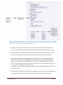
Figure 4 - The ERDDAP search web interface allows one to search for data by specifying multiple criteria.
.................................................................................................................................................................... 28
Figure 5 - Row from an ERDDAP data search for sea surface temperature. .............................................. 29
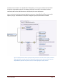
Figure 6 - ERDDAPAqua Modis 8 day sea surface temperature composite. This dataset is accessed using
four dimensions: time, altitude, latitude, and longitude. Positioning the cursor (mouse pointer) over
any one of these will show the possible values and the resolution of the data. ....................................... 30
Figure 7 Detection submission for Matlab client ........................................................................................ 41
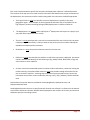
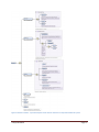
Figure 8– Top level of deployment schema. Light lines indicate optional items. Many of the items
contain subinformation. XML datatypes for each element are denoted in the Type field, and the
constraints indicate elements that are used to form a unique key for a deployment record. .................. 53
Figure 9 – Deployment Sampling Details. Information about each channel of the recording device. Each
channel is assigned a channel number which identifies the channel collected by the instrument. The
SensorNumber provides a link to a specific sensor within the Deployment (Sensors/Audio/Number)
(Figure 11.) .................................................................................................................................................. 55
Figure 10 - Data and QualityAssurance elements. The Data element indicates where audio, tracklines,
and depth sensor information can be found. QualityAssurance permits the annotation of lost or
corrupted data. ........................................................................................................................................... 57
Figure 11 - Description of sensors. Sensors for audio and depth are predefined, and other types of
sensors can be added through the generic Sensor element. ..................................................................... 58
Figure 12 - Ensembles are used to create logical groupings of instrument deployments. ........................ 59
Figure 13- Detection schema. Top level description of how acoustic detections are represented within
the system. .................................................................................................................................................. 61
Figure 14- Detection effort is described by the elements that capture the timespan and types of events
that were investigated. ............................................................................................................................... 62
Figure 15 - Detection elements are repeated within the OnEffort or OffEffort (not shown) elements of a
Detection document to describe observed phenomena. ........................................................................... 63
Tethys Metadata
Page 5
1 Overview
Tethys is a temporal-spatial database for metadata related to acoustic recordings. The database is
intended to house the metadata from marine mammal detection and localization studies, allowing the
user to perform meta analyses or to aggregate data from many experimental efforts based on a
common attribute. This resulting database can then be queried based on time, space, or any desired
attribute and the results can be integrated with external datasets such as NASA’s Ocean Color, lunar
illumination, etc. in a consistent manner. While Tethys is designed primarily for acoustic metadata from
marine mammals, the design is general enough to permit use in other areas as well.
Tethys provides a scientific workbench to the practitioner. Consequently, rather than providing a standalone graphical interface, Tethys provides methods, or subroutines, that can be called from
programming environments that practitioners use to conduct their analysis. Currently, Tethys supports
Matlab, Java, and Python. The R programming language will be included in the next major release.
These methods allow practitioners to access the metadata associated with a specific laboratory or
project. Additionally, the tools provide access to environmental data based on spatial location and
selected temporal boundaries from a wide variety of online sources.
To run Tethys, a Windows machine is required (porting to other platforms is possible with a little work).
To access Tethys from other machines, the network will need to permit communication between
machines. In most cases, this will require a modification of a machine’s firewall rules.
This manual is divided into several major parts and you need not read it all to use Tethys effectively.
Section 2 contains information about installing and administering Tethys, while section 3 provides
information for practitioners who wish to use it. Users may wish to begin by reading about data
organization (section 3.1), the various types of XML documents (section 3.4) and then section of the
manual that is appropriate for the language that they will be using to conduct their queries. Queries can
either be written in the XQuery language (section 3.5) or the user can invoke specialized functions that
construct common queries. The richest set of common queries is available for Matlab (sections 3.7 and
7).
2 Installation and Administration
2.1 Installation
The initial distribution of Tethys is designed to be executed on a Microsoft Windows platform, and a
Windows installer program TethysInstaller.exe is provided. The user will need a Windows machine to be
used as the server1 for creating and housing the database. The same machine can be used for querying
data and using the associated Tethys methods or additional client machines can be used. It is
recommended that there be ample disk space for the database and that plans be put in place for routine
backup of the database. As an example, in early 2014 the database used at the Scripps Whale Acoustics
1
In this context, “server” means that Tethys will be providing services to other machines. The Windows Server
operating system is not required.
Tethys Metadata
Page 6
Lab contained over four million detections and used a bit over 18 GB of storage. The majority of the
space was used for the database records themselves (5 GB) and sample audio and images associated
with detections that were stored at analyst request (11 GB).
During the installation process, the user is first asked what type of installation should be performed
(Table 1). The server code only need be installed on the machine that will be storing the Tethys
database, and it is recommended to do a complete install on the server machine, which will also
initialize a skeleton database for the user. By convention, the installer will place the database in a
subdirectory of C:\Users\Tethys, but this can be overridden this if desired
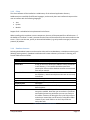
Installation choice
Components installed
Complete Install
Server, Client, initialize a database
Server and database instance
Server, initialize an empty database, and a
populated sample database.
Server only
Server
Server update
Updates the Tethsy project portion of the server
code. This can be used to update to a new version
of the server without having to reinstall Python or
Berkeley DBXML provided that no changes are
needed to those programs (nearly always the
case).
Client only
Client
Empty database
Create a new database instance.
Demonstration database
Create a new database instance that is populated
with sample data.
Empty and demonstration database
Create both databases.
Select server (not yet implemented)
Permits the user to change the default server that
will be accessed by clients. Note that client
programs can override this without changing the
default setting by specifying a server at connection
time.
Table 1 - Types of installations available
Tethys Metadata
Page 7
Individual Windows machines that will be accessing the database can simply install the client software.
Any time the client software is installed, the user will be prompted for the default server. This takes the
form of an Internet machine name (e.g. dataserver.myorg.edu) and a port. Port numbers are a method
of specifying to which service a client should connect. By default, Tethys executed on port 9779, but a
server administrator can change this.
The installer will connect to the Tethys software repository and download and install only the
components that are needed. All of the components are installed as subdirectories of the selected
installation directory.
2.1.1 Quick-start Install for the impatient
Tethys can be run as either a 32 or 64 bit process. This decision must be made at installation time, as
different files are downloaded for each. Your operating system must be a 64 bit operating system in
order to use the 64 bit version of Tethys. In general, the 64 bit version is preferred. It is faster, can
handle larger documents, both for the metadata that your group generates as well as for environmental
data that is retrieved from the Internet.
There is only one instance where one might elect to use the 32 bit version on a 64 bit operating system.
If you wish to import data from Microsoft office applications (e.g. Excel, Access), we recommend
installing the freely available Microsoft Access Engine. There are 32 and 64 bit versions of this library,
and it must match the Tethys architecture. A conflict occurs when a 32 bit version of Microsoft Office is
installed on the Tethys server. The 32 bit Office installs the 32 bit version of the Microsoft Access Engine
and the 64 bit version cannot be installed at the same time. If you need Office on the Tethys server,
either uninstall Office and install the 64 bit version of Office, or install the 32 bit version of Tethys
understanding that there will be performance impacts.
The installer can be started by double clicking on the TethysInstaller executable that can be downloaded
from tethys.sdsu.edu. Should you encounter any problems, please start the installer from the command
prompt by changing directory to the location where the installer was downloaded and typing the
installer name followed by the argument /log=log.txt This will create a log file that will help you (or us)
understand what happened during the installation process.
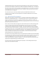
The Tethys installer will present the following series of prompts. The first dialog requests that you
specify where the code will be installed.
Tethys Metadata
Page 8
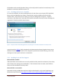
Afterwards, the user will be asked which parts of Tethys should be installed. The default is a complete
install and is the appropriate choice when examining Tethys for the first time.
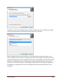
When a database instance is to be installed, you are prompted for the location where data is to be
stored. By default, we store data in C:\Users\Tethys but this can be changed. The default name of the
database will depend upon the type of database instance that is being created. We use metadata as the
default for a new database instance, and demodb for the demonstration database, which contains a
small subset of the Scripps Institution of Oceanography Whale Acoustics Lab’s database Regardless of
the database type, a dialog similar to this one will appear and the data locations and names can be
overridden.
.
Tethys Metadata
Page 9
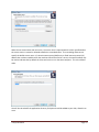
When clients communicate with the server, the server name is required which is either specified when
the server session is started or allowed to default to a standard value. The next dialog allows one to
specify the default server name. If a domain name system (DNS) entry or fixed internet protocol (IP)
address has not been established for the machine that will be used as a server, the name localhost may
be used to indicate that by default the client and server are on the same computer. This is the default
value.
You will also be asked if the application directory for Python should be added to your Path, allow this to
occur.
Tethys Metadata
Page 10
Finally, a summary is produced and pressing install will start the installation process. The process
consists of downloading the needed files, executing separate installers for the dependent programs (use
the default installation values), and unarchiving the remaining programs. Note that the archive
managers may take a minute or two to complete. They will show a blank window and will not show
progress. Some of the archives will take a little while to decompress, especially the Berkeley dbXML
package.
SECURITY NOTE: As the installer cannot know which account will be starting the database, the database
files (not the code) are made writable to any user that can log into the machine on which the database is
running. If this is not acceptable, change the Windows permissions so that only the appropriate account
can modify or access the database.
2.1.2 Server
The server is implemented using two open source technologies: the Python programming language, and
Oracle’s Berkeley DBXML which provides the extended markup language (XML) database engine. The
installer will check to see if the correct version of Python is installed on the machine. If it is missing, it is
downloaded and installed using Python’s own installer. Once the correct version is present on the
machine, add-on libraries are installed and the bindings that permit Python to access the database are
created. Note that if you decide to uninstall Tethys, Python and the Python addons (EGenix, PyWin32,
PyODBC, PyBSDDB, and PyDBXML) will need to be uninstalled separately. If you have another software
package using Python (ArcGIS for example) you should install the Python for use by Tethys in a different
folder than your existing Python folder and may need to.
If data is to be imported into the database from formats other than XML, other programs may need to
be installed. Further details on this can be found in section 3.2.
Tethys Metadata
Page 11
2.1.3 Client
The client software will be installed as a subdirectory of the selected application directory.
Subdirectories are available for different languages, and currently there are interfaces that permit the
user to interface with the following languages:



Java
Python
Matlab
Support for R is scheduled to be implemented in the future.
When installing a client without a server component, the user will be prompted for a default server. If
the default of “localhost” is used, it assumes that the client will be executed on the same machine as the
server. If this is not the case, specify an Internet DNS address (e.g. tethys.nwfsc.noaa.gov) or internet
protocol (IP) address.
2.1.4 Database instance
Selecting the database instance can be used to either add a new database or reinitialize an existing one
(deleting existing entries). Database initialization will create a directory of the user’s choosing, and
several subdirectories and files:
Directory/file
db
source-docs
DeletedArchive
lib
logs
TemporaryFiles
tethys.bat
tethys-ssl.bat
Description
Contains files used by the Berkely DB XML database.
A copy of the source documents added to Tethys are stored
in this directory. This is useful should there ever be a
catastrophic failure and the database need be reconstructed
from source material.
A copy of source documents that have been deleted from
the repository. Note that multiple versions are not currently
maintained.
XQuery library modules and XML schema
Logs detailing server activity.
workspace
A batch file that will launch the Tethys server with the
default options.
A batch file to launch Tethys with secure socket layer
encryption enabled. Note that you must obtain a certificate
and a public/private key pair before you can start Tethys in
this mode. Directions on doing this are in the Tethys secure
socket layer manual that can be found in Tethys/docs folder
relative to your install folder or on the Tethys web site:
tethys.sdsu.edu.
Table 2 - Contents of a database instance
Tethys Metadata
Page 12
The database can be started by double-clicking on the tethys.bat file located in the root directory of the
database or manually as specified in section 2.2
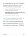
2.1.5 Providing remote access - firewalls
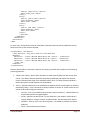
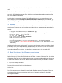
To access your database, you must provide permission for the clients to use the port (9773 by default).
Recent versions of Windows have a built in firewall which must be modified to allow local and/or
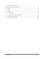
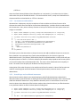
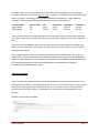
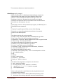
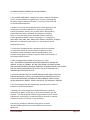
network traffic. The first time you run Tethys, you may see a dialog similar to Figure 1. To permit
connections, click Allow access. Note that this will permit connections from any machine, although your
organization’s firewall may block external access.
Figure 1 – Sample windows firewall dialog (Windows 7) requesting the use to allow connections to the Tethys server.
A tutorial article by Hoffman (2012, also placed in the documentation directory) explains how to set up
Windows firewall rules. The firewall can be configured to provide more selective filtering, such as only
allowing access from specific machines or subnetworks.
2.1.6 Installing Access and Excel support
Microsoft Office installed?
If Microsoft Office Access and Excel are currently installed and they match the architecture (32 or 64 bit)
of the Tethys install, nothing more need be done. If the architecture does not match, either Office or
Tethys must be reinstalled so that they match.
Microsoft Office is not installed
Download the freely available Microsoft Access Engine redistributable. At the time of publication, the
2010 version may be found at http://www.microsoft.com/en-us/download/details.aspx?id=13255. If
Tethys Metadata
Page 13
Microsoft changes their links or if you wish a different version, search for “download Microsoft access
engine” using your favorite search engine.
2.2 Starting the server manually
The database can be started by double-clicking or running dbXMLserver from the command line. The
batch file sets a variable indicating where the Tethys sources were installed and then starts
dbxmlServer.py with the appropriate options.
Several options are available. This list can be seen by using the --help flag on the command line:
c:\Program Files (x86)\Tethys\server> dbXMLserver.py --help
Welcome to Tethys - Server starting...
Usage: dbXMLserver.py - XML Database Server
Default values for choices are marked by an *
Options:
-h, --help
show this help message and exit
-s SECURE_SOCKET_LAYER, --secure-socket-layer=SECURE_SOCKET_LAYER
Use encrypted communication (true/false*)?
encrypted-->https:// unencrypted-->http://
--port=PORT
port to run on (default=9779)
-t TRANSACTIONAL, --transactional=TRANSACTIONAL
Use transaction processing (true*/false)?
-d DATABASE, --database=DATABASE
Directory (folder) name where the XML database will be
stored (must exist). Most users wishing to specify -d
should probably use the -r switch instead.
-r RESOURCEDIR, --resourcedir=RESOURCEDIR
Set Tethys's resource directory (folder). This is the
parent directory for all data used by Tethys including
the XML database.
Each option has a long name that is preceded by two dashes, and sometime a short name which is
preceded by a single dash. Either one may be used.
Setting secure socket layer to true enables encrypted transmission. It requires the generation of
certificates and keys. While the secure socket layer is currently functioning, for this initial manual we
will focus on unencrypted communication as it is much simpler.
Computers communicate across networks by specifying an address and a port. The address is the
Internet protocol (IP) address of the computer running the server and is not settable. The port can be
thought of as a service address at the computer. By default, Tethys uses port 9779, but this can be
overridden.
Many databases are capable of performing operations “atomically.” This means that an operation is
either not performed or is completed, but will never fail in a partially executed way. Should a failure
Tethys Metadata
Page 14
occur part way through an operation (e.g. a power failure), a log is used to either undo the operation or
complete it. This is known as transactional processing and is enabled by default in Tethys.
Files for the database are by default stored in C:/Users/Tethys, but this can be overridden with the
resourcedir option. Several subdirectories are stored relative to the resource directory:






db – The database itself. The name can be overridden with the database option. When the
database flag is used, the folder will be relative to the resource directory unless it contains a
path separator (e.g. –database %USERPROFILE%/Documents/testbed).
DeletedArchive – When files are overwritten, the previous copy is stored here.
lib – Library directory containing schema and database modules
logs – Logs of failure operations.
source-docs - An archive of source material added to the library that can be used for
regenerating the database in case of failure. It also contains any images or short audio clips that
are referenced from the database but not stored directly within it.
TemporaryFiles – Working directory.
Other files may be stored in the resource directory as well. Currently, the file
Detection_Effort_Template.xls is expected to be in the directory.
2.3 Manual shutdown of the server
To shutdown the server, send a terminate command (CTRL+Break, on most keyboards, the break key is
in the row of function keys) and the server will shutdown and the command prompt will close. If users
are using the database, they may lose some data, but the database will not be corrupted.
2.4 Running the server as a service
The server can also be run as an operating system service, although this requires the download of
additional software. The server is started automatically and restarted if the server process unexpectedly
dies or the server machine is restarted. We recommend using the NSSM service manager developed by
Iain Patterson. Source code and executable files can be downloaded from http://iain.cx/src/nssm/ .
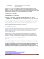
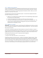
Complete details on NSSM can be found in the NSSM documentation, but to set Tethys as a service you
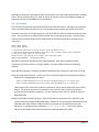
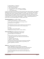
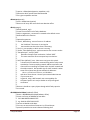
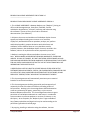
may need to determine if you are using a 32 or 64 bit version of Windows. This can be seen by clicking
on the system properties from the Computer window in Windows 7, other versions of Windows have
similar methods of finding the computer’s properties:
Tethys Metadata
Page 15
Figure 2 - Accessing system properties on a Windows 7 operating system.
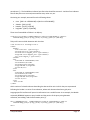
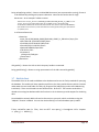
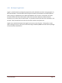
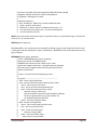
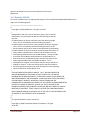
Pressing on System Properties will display a new window that describes the hardware and operating
system. On 64 bit systems, a 64 bit message will be shown:
Figure 3 - The Windows operating system is a 64 bit system if the system type message is present and indicates 64 bits.
Open a command window and type the following for Windows XP systems:
[path-to-nssm]\nssm install Tethys c:\users\Tethys\metadata\tethys.bat start=auto
For Windows Vista and later, change start=auto to start=delayed-auto. Replace [path-to-nssm] with the
folder path to the nssm executable (32 or 64 bit) and change c:\users\Tethys\metadata\tethys.bat if you
have customized where your database resides.
3 Using Tethys
At this point, it is assumed that you have an operational Tethys metadata database. Your database
administrator should be able to tell you the name and port of the machine where Tethys is running.
Tethys uses the extended markup language remote procedure call interface (XMLRPC) to transfer data
between Tethys and the client programming language used for analysis. For common queries, you do
not need to learn XQuery, the language that Tethys’s database uses to access records. A number of
common queries have already been predefined and can be accessed using function calls from one of the
Tethys Metadata
Page 16
Tethys clients. Currently, Matlab has the richest set of queries. For advanced queries, it is helpful to
know XQuery. There is an XQuery tutorial later in this manual. Regardless of whether you use
predefined queries or write your own, it is helpful to understand the structure of how data is stored in
Tethys.
3.1 Data organization in Tethys
Data in Tethys are organized into documents that are placed into containers.
For most of the containers that you are likely to use, a schema is used to define what type of extended
markup language (XML) data can be placed in the container. Parts of the schema are very well defined,
and may require values for certain fields, other parts are loose and allow the user to define new types of
information to be added to the database.
While there are a number of metadata containers in Tethys, the four that we will discuss here are
Deployment, Detections, Localizations, and Ensemble. Each container contains one or more documents.

The Deployments container is used to represent information about the deployment of
instruments used to collect the data analyzed for detection and localization. It contains
information such as the number of channels, sample rate, duty cycle, etc.

The Detections collection describes when events have been detected within a specific
deployment and can be of varying scale. An example of a fine scale detection might be
reporting individual echolocation clicks produces by a Risso’s dolphin while a medium scale
detection might indicate that there was an acoustic encounter of Risso’s dolphins between
some start and end time. Finally, one can report binned presence/absence (e.g. hourly)
information. In addition to the detection events, attachments can be added. These attachments
include audio files and images related to the detections events. Note that a maximum of 500
files can be attached to a given detection document (this limitation will be removed in a future
release).

The Localizations collection denotes the source location of a sound source using either relative
or absolute coordinates and permits the user to reference a detection in the Detections
container if appropriate.

The Ensemble collection allows multiple instruments to be referenced as a single one, which is
useful when performing beamforming or localization on a large aperture array that contains
separate instruments.

The Events collection is used to specify events that may be of interest in the analysis. One such
example might be a planned activity with possible consequences such as oil exploration.
Individual detections of anthropogenic events such as airguns would be recorded in the
Detections collection, but the knowledge that oil exploration was being conducted over a given
time and location could be denoted in the Events collection.
Tethys Metadata
Page 17
Containers are used as needed, for example a set of detections without localizations from a single
instrument would add a document to the Detections and possibly to the Deployment collections, but
would not contribute new entries to the other collections.
Each document is written in extended markup language (XML) which is a language used for structuring
data. The core of XML is quite simple, data is contained within elements that provide structure. The
start of each element is denoted by its name enclosed in < > and the end by the element name within </
>. A small XML fragment is shown below:
<Deployment>
<Project> Socal </Project>
<Deployment> 32 </Deployment>
<Site> A </Site>
<Cruise> SocalInstrument </Cruise>
<Platform> Mooring </Platform>
other entries...
</Deployment>
Units are standardized when recorded in the database. All times follow the ISO 8601:2004 standard and
are recorded in universal coordinated time (UTC). As an example, January 30th, at 6:22:30 PM UTC
would be written 2013-01-30T18:22:30Z. Latitudes and longitudes are recorded in decimal form from
90 degrees (N) to -90 degrees (S) and 0 to 360 degrees (E).
3.2 Adding data to Tethys
Data can be added to the database with XML documents that conform to the schema (p. 53). Ideally,
tools used by researchers will use the Nilus application programming interface to generate XML directly,
but many existing tools generate data in other formats. Consequently, Tethys provides data import
support for the following data sources:




Microsoft Excel workbooks
Comma separated value lists (text files with commas between entries)
Microsoft Access
MySQL open source relational database (www.mysql.com)
Data import services are provided using industry standard open database connectivity (ODBC), and
hence other databases including but not limited to Oracle, Visual Fox Pro, PostgreSQL, etc. should
function, but have not yet been tested. For data sources such as Excel and comma separated value lists,
it is assumed that the first row contains the names of each field. Filenames can contain numbers,
letters, dashes, and periods. Commas in filenames are not supported at this time.
3.2.1
Importing Data to Tethys
Tethys Metadata
Page 18
The Python utility import.py provides data import services, and can be run from any machine that has
network connectivity to the server. Assuming that we wanted to add a set of detections from a
spreadsheet in folder C:/Users/Eloise/SOCAL33M-BeakedWhales.xlsx located on the server machine
tethys.sdsu.edu, with source map SIO.SWAL.Detections.Analyst.v1, we would type at a command
prompt:
import.py --file C:/Users/Eloise/SOCAL33M-BeakedWhales.xlsx --server
tethys.your.org --sourcemap SIO.SWAL.Detections.Analyst.v1 Detections
where
--file indicates the file to be uploaded
--server indicates the server hosting the database. The server name you provided at installation
will be used this option is omitted.
--sourcemap SIO.SWAL.Detections.Analyst.v1 is a translation map, and
Detections is the name of the collection to which we will add C:/…/…BeakedWhales.xlsx
XML translation maps are used to convert between field names used in the data source and names used
in the database. The translators are defined in detail in section 6 (p. 64) but will be briefly introduced in
this section. Each translation map consists of an XML element called Mapping with three children:
Name – Unique name used to specify which mapping should be used. In our example, the map
Name is “SIO.SWAL.Detections.Analyst.v1,” but any name may be used.
DocumentAttributes – This section contains information that will be added to the document so
that the database knows which schema should be used to validate the document. In most
cases, this section should just be copied from one of the existing examples.
Directives – This element contains children that specify how the translation is to be done.
Within the Directives elements, one can specify sheets of a workbook to use or sequential query
language (SQL) queries to databases. Each row of these data sources is then processed
according to the instructions.
The following example is a portion of a Directives element from SIO.SWAL.Detections.Analyst.v1 which
is included in the sample database:
<Map>
<Name> SIO.SWAL.Detections.Analyst.v1 </Name>
<DocumentAttributes> … omissions … </DocumentAttributes>
<Directives>
<Detections>
… omissions …
<OnEffort>
<Sheet name="Detections">
<Detection>
<Entry>
Tethys Metadata
Page 19
<Source> [Input file] </Source>
<Dest> Input_file </Dest>
</Entry>
<Entry>
<Source> [Start time] </Source>
<Kind> DateTime </Kind>
<Dest> Start </Dest>
</Entry>
<Entry>
<Source> [End time] </Source>
<Kind> DateTime </Kind>
<Dest> End </Dest>
</Entry>
… omissions …
</OffEffort>
</Detections>
</Directives>
</Map>
For each row in the Detections sheet of a workbook, a Detection element will be produced as shown
below with many of the elements omitted:
<ty:Detections …attributes…>
… many omissions, only Start shown for each Detection …
<OnEffort>
<Detection> … <Start> 2012-06-01T14:50:22.52Z </Start> … </Detection>
<Detection> … <Start> 2012-06-01T14:50:23.9Z </Start> … </Detection>
<Detection> … <Start> 2012-06-01T14:50:41.32Z </Start> … </Detection>
… other rows …
</OnEffort>
</ty:Detections>
Elements nested within a <Directives> element are simply copied with the exception of the following
processing elements:


<Sheet> and <Table>: Both of these elements are used to specify data from the current data
source. The <Sheet> directive should be used with spreadsheets and expects the attribute
name to indicate which sheet of the workbook will be used. For Table, the query attribute is
used and may be any valid SQL query for the database.
<Entry>: Specifies how fields in the spreadsheet or database will be transformed to an element
expected by Tethys. <Entry> elements are always children of <Sheet> or <Table> elements and
contain children describing the translation:
o <Source>: One or more field names enclosed in square brackets [ ]. Multiple fields can
be specified and will be merged together.
o <Kind>: Specifies the data format. For text fields this is not needed. Valid kinds are:
LongLat, DateTime, Integer, Number, and SpeciesCode. See the appendix for details.
o <Default>: Value to use in cases of missing data. If no default is provided, no value is
produced.
o <Dest>: Name of the output element.
Tethys Metadata
Page 20
3.2.2 Updating existing documents
We do not encourage modifying existing data by modifying the database. Rather, modify the document
that was submitted and import it again with overwrite enabled (see previous section).
The rationale for this is that a copy of each source document submitted to Tethys is saved in addition to
submitting the database. The documents are stored in the subfolder of the database’s source-docs
folder2 that corresponds to the collection name. This makes is possible to rebuild the entire database
should there be a case of catastrophic failure.
To rebuild a collection, use the Python client program update_documents.py. The following is an
example where any document that was inadvertently removed from SourceMaps is re-added:
update_documents.py SourceMaps
In general, any number of collections can be listed to be updated. Alternatively,
update_documents.py --update=true all
can be used to update all collections. The –update=true flag indicates that existing documents should
be replaced by their sourcedocs collection document. This is not usually needed unless one has done a
global search and replace across source documents and wishes to incorporate the modified documents
into the database. Finally, the optional --clear flag will have the same effect as running the
clear_documents.py command prior to update_documents.py (see the following section).
3.3 Removing data from Tethys
Individual documents may be removed as outlined in section 3.8.1.4 (p. 43). An entire collection can be
emptied using the clear_documents.py command executed from the command line. The syntax is as
follows:
clear_documents.py collection1 collection2 ...
Clear documents in the specified collections.
This will not remove any source documents used to build the collection,
but it will remove ALL documents from the specified collections and
should be used with caution.
Options:
-h, --help
show this help message and exit
-s SECURE_SOCKET_LAYER, --secure-socket-layer=SECURE_SOCKET_LAYER
Use encrypted communication (true*/false)?
encrypted-->https:// unencrypted-->http://
--port=PORT
port to run on (default=9779)
2
An exception to this is when the source material comes from a database.
Tethys Metadata
Page 21
--server=SERVER
Server name (defaults to 132.239.122.177
(beluga.ucsd.edu))
The primary use for this is prior to updating a collection whose contents come from an external
database. As an example, at the Scripps Whale Acoustics Lab, a MySQL database is used to track the
deployments of our instruments. Rather than trying to determine which deployments have been added
to Tethys, and only add the new ones, we simply empty the Deployments container:
clear_documents.py Deployments
followed by an import of the Deployments:
import.py --file HarpDB --sourcemap SIO.SWAL.Deployments.v1 --server
tethys.my.org --connectionstring "Server=harp.my.org;Port=3306;User=harpuser;Password=*" Deployments
where the MySQL database is running on machine harp.my.org on port 3306, and Tethys is running on
tethys.my.org. MySQL will be accessed with account harp-user. Setting Password to * will result in
import.py prompting for a password. Data will be imported to the Deployments collection from
database HarpDB using the SIO.SWAL.Deployments.v1 sourcemap.
3.4 XML Document types
The Tethys schema support several types of documents that are described at a high level in this section.
The goal is to describe the types of information contained in the documents rather than every last
detail. More detailed descriptions can be found in appendix 5 which describe the schema that
structures each document type.
Where possible, we use concepts from ISO 19115 or OpenGIS SensorML3, but our emphasis is on
meeting the needs of the marine mammal community in the most user-friendly way possible. As a
consequence, we deviate from these standards. In addition, there are many concepts that are not
covered in these standards such as recording detection effort.
3.4.1 ITIS
The itis collection contains one document, which is a subset of the integrated taxonomic information
system (ITIS, www.itis.gov). While the Python tool update_documents.py is capable of converting any
subset of the ITIS database to XML, the default database contains an ITIS subset suitable for
oceanographic work. It contains marine mammals from the order Cetacea (whales and dolphins) and
the suborder Caniformia (sealions and seals). Fish from families Sciaenidae (drums or croakers),
Cottidae (sculpin), Sebastidae (rockfishes, rockcods and thornyheads), class Actinopterygii (ray-finned
fishes), and superclass Osteichthyes (bony-fishes) are also included. Note that while only a subset of ITIS
3
http://www.iso.org/iso/catalogue_detail.htm?csnumber=26020 and
http://www.opengeospatial.org/standards/sensorml respectively
Tethys Metadata
Page 22
has been included, it is possible to add any species represented by ITIS4. Each entry has a taxonomic
serial number (TSN), completename (scientific name), and vernacular entries.
Tethys’s XML representation of ITIS supports physical phenomena by defining them with negative
taxonomic serial numbers. Currently, there is a single TSN entry, Other, for physical phenomena. Due
to the structure of the Tethys schema, the other category is represented as a Kingdom which is of course
incorrect.
3.4.2 Deployment documents
Each document in the Deployments collection describes a deployment of an instrument. As many
instrument designers have existing databases for their instruments, the goal in the deployment
documents is to provide enough information to access an instrument database and then to describe
how the instrument was used. Information such as how and where an instrument was deployed,
references to tracklines for moving platforms, sensor packages and configuration are all described here.
While the emphasis is on acoustic data (e.g. sampling rates, duty cycles, quantization), the schema
permit the description of arbitrary instrumentation.
3.4.3 Detection Documents
Detection documents record information about the process used to perform the detections, the source
data, and the effort which indicates which species and calls were searched for in the detection process.
Recording effort is essential as the lack of detections for a specific species/call type is not relevant unless
one was actually looking for them.
An essential element for being able to conduct metastudies is to use consistent naming conventions. To
that end, we have adopted the integrated taxonomic information system (ITIS, www.itis.gov) for
describing species. As the taxonomic serial numbers (TSNs) used by ITIS are not user friendly (180514 is
the TSN for Stejneger’s beaked whale, Mesoplodon stejnegeri), library functions permit the translation
between TSNs and common or scientific names. In addition, a SpeciesAbbreviations collection permits
labs to use their own set of local names or abbreviations (see 6.2 for details). Like the translation maps
described in section 3.2, these are XML documents that provide mappings between a local name or
abbreviation and the Latin species name which permits automatic bidirectional translation. Details on
the translation are described in section
A list of call types has is being established based on the literature5. The DetectionEffortTemplate
spreadsheet found in the root folder of the sample database contains a list of the species and call types.
We do not currently enforce the use of these names in Tethys, but rather recommend doing so in any
detection software that is used to generate detections to be stored in Tethys.
When possible, we recommend that detectors generate XML conforming to the Tethys schema (section
5), however it is not uncommon to want to import detections from an already established format. Most
such formats can be thought of as tables and facilities exist to import them from comma separated
4
Doing so requires running a copy of the ITIS database on your machine and making modifications to the last few
lines of the itis_order.py Python program.
5
This process has been completed for mysticetes and is in progress for odontocetes.
Tethys Metadata
Page 23
value lists, spreadsheet workbooks, and a wide variety of database products. Regardless of the data
source, a common issue is how the data source, with its own organization and field names, can be
translated into the XML required by Tethys. Section 3.2 describes data import at a high level and section
6 describes how to specify the mapping between a row oriented data source and XML documents.
3.4.4 Localization documents
Localization documents provide location information in the form of absolute locations or bearings.
Localizations can be derived from data sources consisting of a single instrument deployment or an
ensemble of multiple instrument deployments.
Like detection documents, localization documents begin with a description of the localization process
followed by identification of the data source, the algorithm and its parameters as well as the user who
submitted the localizations. This is followed by a description of the zero location. All localizations are
made relative to this point which may be in absolute coordinates (e.g. UTM or longitude and latitude) or
relative to the deployment or ensemble.
Each localization has a set of metadata about the localization. An event identifier uniquely identifies the
event within the current document. A selection element permits the localization to be related to a
specific detection or to a time-frequency bounding box relative to one of the channels. Finally, a list of
sensors is provided that indicates which of the available sensors were used in this specific localization.
The localization data itself consists of either a bearing or a location. Bearings consist of a horizontal and
optional vertical angle, specified in degrees. Locations are x, y, and optional z distances, specified in
meters relative to the zero location. For either type of localization, standard error may be specified in
the same units. Finally, when a location is a result of several crossed bearings, an optional list of
bearings (event identifiers from previous localizations) may be provided to link the position to the
bearings used to produce it.
3.4.5 Events
The events collection is designed to denote phenomena or events that are derived from other
knowledge sources. Examples of this include planned Naval exercises, whale watching cruises, pile
driving, oil exploration, earthquakes, etc. This collection is experimental and requires more community
input before a definitive schema is designed.
3.4.6 External document types
Tethys provides the ability to access external data sources which are represented as collections prefixed
with the name ext: followed by a collection name. Tethys provides what is known as a mediation
service, providing a consistent way of accessing these external data sources. These are returned as XML
documents that can be manipulated like any other data that Tethys returns.
Data access is constructed in a manner that looks similar to XML document navigation. The user
specifies the collection they want followed by a set of slash (/) separated parameters and terminated
with an exclamation point:
collection("ext:MediatorServiceName")/parameter1/.../parameterN!
Tethys Metadata
Page 24
Currently, mediation is provided for several types of external container types described in the following
sections.
When Tethys accesses an external collection, it caches the results for approximately seven days (default)
on the Tethys server. Consequently, if the same data is requested multiple times, subsequent queries
are faster. This is particularly helpful when developing routines to analyze data where the same query
may be executed dozens of times as the analysis routine is written. The cached results are stored in
collection mediator_cache. In rare cases, one may wish to disable this behavior. Examples of this
include services that provide different results for the same parameters (e.g. report current conditions)
and when one knows that a service has been recently corrected.
There are two ways to ensure that mediated services retrieve values directly from the Internet. The first
is simply to add a colon followed by cacheupdate after the mediation service name, e.g.
collection("ext:MediatorServiceName:cacheupdate")/parameter1/.../parameterN!
Data are retrieved from the mediator service and the mediator cache will be updated with the new
results. A second and more drastic way to clear the cache is to empty the mediator_cache collection
using one of the client programs such as the Python client’s clear_documents.py . Both methods will
work, but emptying the mediator_cache clears the cache of all documents for every user, so the
cacheupdate parameter is usually the preferred mechanism for ensuring a fresh copy of the data.
3.4.6.1 Ephemeris data
Ephemeris, information about astronomical objects, can be obtained through an interface to NASA JPL’s
Horizons Web Service (Giorgini et al., 1996). While NASA’s system provides information on a variety of
astronomical objects, the mediator interface has been primarily tested for solar and lunar information.
The Horizons service is accessed via the ext:horizons collection. An example query might look like this:
collection("ext:horizons")/target="sol"/latitude=32.8/longitude=243.8/start="2009-10-01T00:0008:00"/stop="2009-10-04T00:00-08:00"/interval="5m tvh"!
The arguments may appear in any order and are as follows:




target – Celestial body. The horizons mediator knows the names “sol” and “sun” for the sun,
“moon” and “luna” for the moon.
latitude and longitude – Position of the location in degrees for which the ephemerides are to be
computed. Latitude must be in the interval between 90° (N) and -90° (S), and longitude must be
between 0 and 360° E. Note that this is the format in which Tethys stores latitude and longitude
and no conversion is needed.
start and stop – Time in ISO8601 format (YYYY-MM-DDTHH:MM:SS). All times are assumed to
be in universal coordinate time (UTC) which again is the Tethys default.
interval – How often should the ephemeris be computed. When determining transit (rise/set),
this should be in intervals of 5 m with the tvh flags set as in the example above.
Tethys Metadata
Page 25
Tethys will return XML describing the ephemerides. The document consists of a set of entries describing
information about the celestial object in question. The result of the query above with manually added
comments is:
<?xml version="1.0" encoding="utf-8"?>
<ephemeris>
<entry>
<date>2009-10-01 01:35:00</date>
<sun type="civil">day</sun>
<!-- Civil sunset -->
<moon>set</moon>
</entry>
<entry>
<date>2009-10-01 13:44:00</date>
<sun>day</sun>
<moon>rise</moon>
</entry>
<entry>
<date>2009-10-01 19:38:00</date>
<sun>day</sun>
<moon>transit</moon>
</entry>
<entry>
<date>2009-10-02 01:32:00</date>
<sun type="civil">night</sun> <!-- Civil sunrise -->
<moon>set</moon>
</entry>
<entry>
<date>2009-10-02 13:41:00</date>
<sun>day</sun>
<moon>rise</moon>
</entry>
<entry>
<date>2009-10-02 19:35:00</date>
<sun>day</sun>
<moon>transit</moon>
</entry>
<entry>
<date>2009-10-03 01:29:00</date>
<sun type="civil">night</sun>
<moon>set</moon>
</entry>
<entry>
<date>2009-10-03 13:43:00</date>
<sun>day</sun>
<moon>rise</moon>
</entry>
<entry>
<date>2009-10-03 19:37:00</date>
<sun>day</sun>
<moon>transit</moon>
</entry>
</ephemeris>
Note that in most cases, information about the moon is returned as well.
Tethys Metadata
Page 26
3.4.6.2 Timezone data
The time zone collection can provide time zone for a specific longitude and latitude based on nautical
time zones that consist of 15° gores centered on the prime meridian or based on civil boundaries. In
general, the nautical gores are preferred as the civil boundaries are from a community effort maintained
at earthtools.org and may be subject to error. An example of a nautical time zone query (the default)
is:
collection("ext:timezone")/latitude=32.8/longitude=243.8!
Arguments can appear in any order and are:


longitude and latitude – Position of the location in degrees for which the timezone is to be
computed. Latitude must be in the interval between 90° (N) and -90° (S), and longitude should
be between 0 and 360° E although the mediator will also take degrees west as a negative
number. Note that this is the format in which Tethys stores latitude and longitude and no
conversion is needed.
tztype – Must be “nautical” or “civil,” nautical is the default if omitted. Use civil with extreme
caution as it has not been well verified.
The query above produces the following XML.
<?xml version="1.0" encoding="utf-8"?>
<timezone xmlns:xsi="http://www.w3.org/2001/XMLSchema-instance"
xsi:noNamespaceSchemaLocation="http://www.earthtools.org/timezone-1.1.xsd">
<version>1.1</version>
<location>
<latitude>32.800000</latitude>
<longitude>-116.200000</longitude>
</location>
<offset>-8</offset>
<suffix>U</suffix>
<localtime/>
<isotime/>
<utctime/>
<dst>Unknown</dst>
</timezone>
In most cases, the element of interest in a timezone query is the offset which in this case is -8 hours
from UTC.
3.4.6.3 NOAA ERDDAP data
NOAA’s Environmental Research Division Data Acccess Program (ERDDAP) provides a method of
accessing a wide variety of environmental and biological data. ERDAP provides code to access most
environmental data directly, but using the Tethys interface permits the queries to be driven by results of
other queries. In addition, the next release of Tethys will support caching of external queries at the
server. The impact of this is that during development of research code, users frequently make the same
query over and over again. By maintaining a cache at the server which in most cases is on the local area
Tethys Metadata
Page 27
network, the retrieval time is likely to be significantly faster on subsequent queries. In addition, it
reduces the load on remote servers.
ERDAP organizes data either as a grid or a table and uses data access protocols named Griddap and
Tabledap respectively. Latitude and longitudes follow the same conventions as Tethys, latitude is
expressed in degrees North and longitude in degrees East.
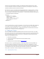
The first step in using ERDDAP is to decide what type of data is to be used and then to find an
appropriate data set. We will begin by looking for sea surface temperature. Throughout this section,
we will use examples from the Matlab client (section 3.7). In this example, we will begin by looking for
sea surface temperature and assume that we do not know anything about ERDDAP’s naming
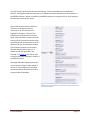
conventions. Consequently, we begin by invoking dbERDDAPSearch with no search parameters:
dbERDDAPSearch(queryH);
% Assumes that queryH = dbInit() has been executed
This function returns the URL of the ERDDAP search page, but more importantly opens a web browser
that allows one to search for a desired dataset. The ERDDAP search page allows full text search as well
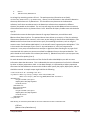
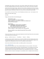
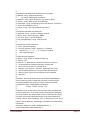
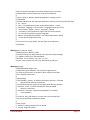
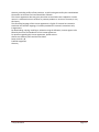
as search by a number of categories as well as by geo-temporal constraints. In our case, we will use the
keywords category to search for sea_surface_temperature:
Figure 4 - The ERDDAP search web interface allows one to search for data by specifying multiple criteria.
Geographic constraints can be found by specifying a bounding box either in the boxes or by dragging a
rectangle on the map. Time constraints are specified in the ISO 8601:2004 time format used by Tethys
Tethys Metadata
Page 28
(e.g. 2013-01-30T18:22:30Z). After pressing the Search button, the results will show a list of datasets
meeting the specified criteria.
Each dataset has a unique identifier (ID) that will be used in all queries involving that dataset. In this
case, we will select NOAA Coastwatch’s one day SST composite: erdGRssta1day.
As one learns the search vocabulary, it becomes relatively simple to search for specific datasets from the
command line. Each of the search parameters are joined by ampersand (&). The following Matlab and
XQuery statements both find the URL for a region within approximately 5 km of an instrument deployed
on the south east side of the Santa Cruz Basin in the Southern California Bight:
dbERDDAPSearch(queries, 'keywords=sea_surface_temperature&minLat=33.47&maxLat=33.56&
minLong=240.71&maxLong=240.80')
Although not covered until the section on the XQuery language, it is worth noting that this Matlab
function simply translates the search to an XQuery which returns a URL that is then opened by the
Matlab function:
collection("ext:erddap_search)/keywords=sea_surface_temperature&minLat=33.47&maxLat=33.56&
minLong=240.71&maxLong=240.80!
Once the ERDDAP data set has been identified, it can be queried to retrieve the data. In this example,
we will assume that a one day composite sea surface temperature would suffice and will use the NOAA
Coastwatch eight day composite sea surface temperature dataset from the Aqua MODIS satellite which
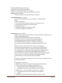
has the dataset identifiier erdMBsstd1day. When we locate this dataset in the web page, we see that
the data is listed in the Griddap column indicating that we should expect gridded data to be returned
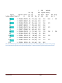
(Figure 5).
Institution
Dataset ID
NOAA
CoastWatch
erdMWsstd8day
background
E-mail
Background Info
F I M
RSS
FGDC,ISO,Metadata
graph
data
SST, Aqua MODIS,
NPP, West US, Daytime
(8 Day Composite)
Summary
Title
WMS
Make A Graph
Table DAP Data
Sub-set
GridDAP Data
M
Figure 5 - Row from an ERDDAP data search for sea surface temperature.
Tethys Metadata
Page 29
Other sources, such as buoys, might be expected to return tabular or vector data as shown in the
Tabledap column.
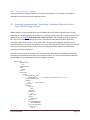
Clicking on the data link (Figure 5) exposes more information about the dataset (Figure 6). It shows the
dimensions of the dataset indices. To query this dataset, we need to specify four sets of indices: time,
altitude, latitude, and longitude. The minimum and maximum values of the dataset can be seen by
moving the cursor over the dimension or in the more detailed data attribute structure which is shown
beneath the sliders although it has not been reproduced here.
Figure 6 - ERDDAPAqua Modis 8 day sea surface temperature composite. This dataset is accessed using four dimensions:
time, altitude, latitude, and longitude. Positioning the cursor (mouse pointer) over any one of these will show the possible
values and the resolution of the data.
The sea surface temperature variable is called sst as shown in the Grid Variables section (Figure 6). To
construct a query, we need to specify the following:



dataset identifier, erdMWsstd8day in this example
the variable(s) to be returned, sst,
and a list of dimensions.
Each dimension is enclosed in square brackets, [ ], and this dataset will require four sets of these. Each
set of brackets has the following syntax: [StartValue:StrideValue:StopValue] The values may either be
indices from 1 to the number of grid points, or in the units associated with the grid axis (e.g. time,
longitude, etc.). When values are specified in units as opposed to indices, they must be enclosed in
Tethys Metadata
Page 30
parentheses ( ). The StrideValue indicates how often data should be returned. A stride of one indicates
that all data points are returned, two would be every other one, etc.
Continuing our example, we would have the following values:




time: [(2012-11-13T00:00:00Z):1:(2012-11-13T00:00:00Z)]
altitude: [(0.0):1:(0.0)]'
latitude: [(33.47):1:(33.59)]
longitude: [(240.7):1:(240.80)]
These are all assembled as follows in an XQuery:
collection("ext:erddap")/erdMWsstd8day?sst[(2012-11-13T00:00:00Z):1:(2012-1113T00:00:00Z)][(0.0):1:(0.0)][(33.47):1:(33.59)][(240.7):1:(240.80)]!
Tethys will return an XML document with the data:
<?xml version="1.0" encoding="utf-8"?>
<table>
<header>
<time units="UTC" type="String"/>
<altitude units="m" type="double"/>
<latitude units="degrees_north" type="double"/>
<longitude units="degrees_east" type="double"/>
<sst units="degree_C" type="float"/>
</header>
<row>
<time>2012-11-13T00:00:00Z</time>
<altitude>0.0</altitude>
<latitude>33.475</latitude>
<longitude>240.7</longitude>
<sst>16.83</sst>
</row>
<row>
<time>2012-11-13T00:00:00Z</time>
<altitude>0.0</altitude>
<latitude>33.475</latitude>
<longitude>240.7125</longitude>
<sst>16.77</sst>
</row>
… more entries
</table>
which consists of a header element describing the data and the units in which they are represented.
Following the header is a series of row elements, where each element describes a grid point.
Language specific interfaces will parse this information into a usable format. As an example, the Matlab
command dbERDDAP expects a query handler and the portion of the query string between
collection("ext:erddap)/ and the exclamation point (!):
data = dbERDDAP(queries, 'erdMWsstd8day?sst[(2012-11-13T00:00:00Z):1:(2012-1113T00:00:00Z)][(0.0):1:(0.0)][(33.47):1:(33.59)][(240.7):1:(240.80)]')
data =
Tethys Metadata
Page 31
hdr:
time:
altitude:
latitude:
longitude:
sst:
[5x1 struct]
{90x1 cell}
[90x1 double]
[90x1 double]
[90x1 double]
[90x1 double]
When requesting ERDDAP data, it is currently returned as columnar data regardless of whether the
dataset was produced by GRIDDAP or TABLEDAP. This can be reshaped into matrix format by using the
Matlab dbERDDAPReshape function. Future releases will do this automatically. The user must specify
the number of axes in the dataset:
grid4D = dbERDDAPReshape(data, 4)
grid4D =
hdr:
time:
altitude:
latitude:
longitude:
sst:
labels:
[5x1
{4-D
[4-D
[4-D
[4-D
[4-D
[1x1
struct]
cell}
double]
double]
double]
double]
struct]
If we wished to see sea surface temperature from the first day, grid4D.sst(1,1,:,:) could be used.
Unfortunately, Matlab remembers that this is the third and fourth dimension of a four dimensional
matrix, and using the data in this format is difficult. The data can be reduced to a standard matrix with
the squeeze command:
squeeze(grid4D.sst(1,1,:,:))
which removes singleton dimensions.
3.5 XQuery
XQuery is a language used to query XML databases. Walmsley’s (2006) book on XQuery provides an
excellent and complete introduction to XQuery and is recommend reading for people who wish to
become experts in XQuery. Many useful queries can be performed using the Matlab client with no
knowledge of XQuery whatsoever. However, for users who wish to create complicated custom queries,
investing the time to learn XQuery will be beneficial. Our goal in this section is to provide a gentle and
incomplete introduction to XQuery, deferring advanced materials to other sources such as Walmsley’s
book.
3.5.1 Our first query
It is helpful to run queries interactively when designing them, and the Matlab interface provides a good
way to do this. The Matlab client is described in section 3.7, and the Matlab function dbRunQueryFile()
is particularly helpful. We begin with a query to find all deployments where effort has been put into
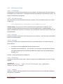
finding Pacific white-sided dolphin clicks:
import schema namespace ty="http://tethys.sdsu.edu/schema/1.0" at "tethys.xsd";
Tethys Metadata
Page 32
<ty:Result xmlns:xsi="http://www.w3.org/2001/XMLSchema-instance">
{
for $detections in collection("Detections")/ty:Detections
(: 180444 is the Pacific white-sided dolphin :)
(: We'll see how to find this automatically later :)
where $detections/Effort/Kind/SpeciesID = 180444
return
<Effort>
{$detections/DataSource}
</Effort>
}
</ty:Result>
The query begins with an import statement. This is required for nearly every Tethys query and defines
what is known as a namespace. Namespaces can be thought of as prefixes that can distinguish elements
with the same name. As an example, the first element in a Tethys detections document is Detections.
To distinguish this from other possible Detections documents established by other groups, we associate
it with a namespace. The namespace used by Tethys is http://tethys.sdsu.edu/schema/1.0. The first
import statement:
import schema namespace ty="http://tethys.sdsu.edu/schema/1.0" at "tethys.xsd";
states that we will abbreviate the namespace as “ty,” and provides a hint to the XML database as to
where the schema definition will reside (at file tethys.xsd on the server). Top-level elements within the
Tethys schema can now be denoted with a ty: prefix, e.g. <ty:Detections>. Note that there is nothing
special about the choice of the abbreviation ty, it is the namespace itself,
http://tethys.sdsu.edu/schema/1.0, that is important.
XQueries return XML documents. One strategy in designing XQueries is to design a document skeleton
and have XQuery fill in portions of it. Tethys provides a generic document element called <Result>
whose schema permits any valid XML, and we note that the XML is bracketed by:
<ty:Result xmlns:xsi="http://www.w3.org/2001/XMLSchema-instance">
…
</ty:Result>
The xsi namespace declared in <ty:Result> is not mandatory, but it will prevent the children of
<ty:Result> from having the xsi namespace in each element. The namespace is present in Tethys
documents as they reference a schema which is part of the http://www.w3.org/2001/XMLSchemainstance namespace. To distinguish the XQuery code from the XML document, curly braces { } are used
and we see that { } brackets the XQuery code in our query.
Let us turn our attention to the XML code itself which we number for convenience:
1. for $detections in collection("Detections")/ty:Detections
2.
(: 180444 is the Pacific white-sided dolphin :)
3.
(: We'll see how to find this automatically later :)
4.
where $detections/Effort/Kind/SpeciesID = 180444
Tethys Metadata
Page 33
5.
6.
return
$detections/DataSource
Let us begin by examining portions of line 1. The path expression (referred to as an XPath),
collection("Detections")/ty:Detections, returns a list of documents in the collections detection
whose top-level element is <ty:Detections>. This should be every document in the Detections
collection, but if there were documents in the Detections collection that started with a different
element, they would not be included. The for loop will assign the variable $detections to each one
of these documents at the <ty:Detections> level. Note that all XQuery variables start with the dollar
sign ($).
If we wished to access the Description element for a group of detections, we could do so with
$detections/Description. The optional where clause allows us to restrict, or filter, the selection
of documents based on their contents. In this case, we are looking for Pacific white-sided dolphins, TSN
180444 and will see later how we could write a query for something less obscure, such as using the
common name “Pacific White-sided Dolphin” or the scientific name “Lagenorhynchus obliquidens.” This
is also noted in the comments of lines 2 and 3. Any text between a (: and :) are interpreted as
comments. In any case, to find effort where analysts or algorithms were searching for any type of call
associated with this species, we construct an XPath from $detections to the species identifier. The
path is based on the structure of the schema (see section 5), $detections/Effort/Kind/SpeciesID,
and has a check for equality (line 4).
For each document that remains after our filter for Pacific white-sided dolphins, we wish to return
information about the data source. This is indicated by the return statement on line 5 which is followed
by either an XQuery expression or XML. In the above example, it is followed by an XQuery expression
that states that the DataSource element and its children which specify the project, deployment, and site
should be returned. A sample output might look like the following:
<?xml version="1.0" encoding="utf-8"?>
<ty:Result xmlns:ty="http://tethys.sdsu.edu/schema/1.0"
xmlns:xsi="http://www.w3.org/2001/XMLSchema-instance">
<DataSource>
<Project>SOCAL</Project>
<Deployment>40</Deployment>
<Site>M</Site>
</DataSource>
many entries omitted…
<DataSource>
<Project>SOCAL</Project>
<Deployment>44</Deployment>
<Site>N</Site>
</DataSource>
</ty:Result>
Alternatively, we could have placed XML in the return statement and line 5 could have read:
<Effort>
{$detections/DataSource}
Tethys Metadata
Page 34
</Effort>
where the XPath element $detections/DataSource is enclosed in { } to indicate that it is XQuery
code rather than part of the XML document. The result would be similar, except each <DataSource>
element would be enclosed within an <Effort> element.
3.5.2 Let statements and modules
We extend our simple query with the introduction of other variables and a library function call to
eliminate the need to know the TSN for Pacific white-sided dolphins. Variables can be introduced with
the let statement. Here, we use a library function to look up the TSN from the Latin species name and
assign it to a variable:
1. import schema namespace ty="http://tethys.sdsu.edu/schema/1.0" at "tethys.xsd";
2. import module namespace lib="http://tethys.sdsu.edu/XQueryFns" at "Tethys.xq";
3.
4.
5.
6.
7.
8.
9.
10.
11.
12.
<ty:Result xmlns:xsi="http://www.w3.org/2001/XMLSchema-instance">
{
(: Find TSN from species name :)
let $id := lib:completename2tsn("Lagenorhynchus obliquidens")
for $detections in collection("Detections")/ty:Detections
where $detections/Effort/Kind/SpeciesID = $id
return
$detections/DataSource
}
</ty:Result>
This XQuery returns the same values as the previous ones, but adds an additional import to access the
library module in the namespace http://tethys.sdsu.edu/XQueryFns (line 2) which is given the
abbreviated name lib. The lookup is performed by function completename2tsn in line 6 which will map
the species name to a TSN if it is in the itis collection (all cetaceans and pinnipeds as well as many fishes
are in the ITIS subset that are distributed with ITIS). The value is then substituted into the equality of
line 8. The results from this query will be identical to the previous one.
A description of the other functions in the module can be found in section 8. Most of the functions are
useful for translating back and forth between TSNs and species names, common names, or local
abbreviations.
3.5.3 Nested loops and conditional statements
We continue this with a slightly more complicated query which finds the detections themselves in
documents where we know that we are looking for Pacific white-sided echolocation clicks. Note that we
could have looked for detections in every Detection document, but it is more efficient to restrict our
search to places where detection effort has been made as there should not be any on-effort detections
in any document where no effort has been placed in finding them.
1.
2.
3.
4.
5.
6.
import schema namespace ty="http://tethys.sdsu.edu/schema/1.0" at "tethys.xsd";
import module namespace lib="http://tethys.sdsu.edu/XQueryFns" at "Tethys.xq";
<ty:Result xmlns:xsi="http://www.w3.org/2001/XMLSchema-instance">
{
let $id := lib:completename2tsn("Lagenorhynchus obliquidens")
Tethys Metadata
Page 35
7.
8.
9.
10.
11.
12.
13.
14.
15.
16.
for $detections in collection("Detections")/ty:Detections
where $detections/Effort/Kind/SpeciesID = $id
return
for $d in $detections/OnEffort/Detection
where $d/SpeciesID = $id and $d/Call = "Clicks"
return if ($d/Parameters/Subtype)
then $d
else ()
}
</ty:Result>
This example begins in a similar manner to the first one, but begins to differ in what is returned starting
at line 10. The return value is actually a nested XQuery. Once we have identified a document where
there was effort for Pacific white-sided echolocation clicks, we look through the on-effort detections
(line 10), and then filter out all calls that were not Pacific white-sided echolocation clicks (line 11). As
this is a nested XQuery, it also needs a return value. Rather than returning every detection, we wish to
only return echolocation clicks that have a subtype associated with them. In Soldevilla et al. (2008), we
identified two types of echolocation clicks which we called subtypes A and B. We store this distinction in
Tethys by adding a <Subtype> element as a child of <Parameters>.
The if statement on line 12 is true if there is a Parameters/Subtype element relative to the current
detection, $d. When this is true, the detection is returned, otherwise the empty sequence is returned
which does not change the output. The following shows a sample output from this query:
<?xml version="1.0" encoding="utf-8"?>
<ty:Result xmlns:ty="http://tethys.sdsu.edu/schema/1.0"
xmlns:xsi="http://www.w3.org/2001/XMLSchema-instance">
… many detections omitted …
<Detection>
<Input_file>H:\SOCAL44N_disk06\SOCAL44N_disk06_5s_100Hz.ltsa</Input_file>
<Start>2011-08-17T02:58:12.500Z</Start>
<End>2011-08-17T03:18:02.500Z</End>
<Event>02/28/12 13:05:56</Event>
<SpeciesID>180444</SpeciesID>
<Call>Clicks</Call>
<Parameters>
<Subtype>A</Subtype>
</Parameters>
</Detection>
<Detection>
<Input_file>H:\SOCAL44N_disk07\SOCAL44N_disk07_5s_100Hz.ltsa</Input_file>
<Start>2011-09-15T02:49:27.500Z</Start>
<End>2011-09-15T03:18:17.500Z</End>
<Event>03/02/12 10:58:35</Event>
<SpeciesID>180444</SpeciesID>
<Call>Clicks</Call>
<Parameters>
<Subtype>A</Subtype>
<UserDefined>
<peak_1_low>21700.0</peak_1_low>
<peak_2>27700.0</peak_2>
<peak_3_high>38400.0</peak_3_high>
</UserDefined>
</Parameters>
</Detection>
</ty:Result>
Tethys Metadata
Page 36
Although not shown here, the order by clause can be used to sort results and typically follows the where
clause. Due to the keywords for, let, order by, where, and return, queries in the XQuery language are
frequently referred to as FLOWRs (pronounced flowers).
3.6 Java client
The Java client provides basic functionality and consists of two Java classes. The Client class represents
client information about the Tethys server, and the Queries class provides an interface to the server.
The Client constructor has a single argument, a URL which will be used to communicate with the Tethys
server. This can either be an instance of the java.net.URL or java.lang.String classes. Once the client is
created, one can create a Queries instance which takes an instance of Client as the argument to its
constructor:
import dbxml.Client;
import dbmxl.Queries;
// Initialize connection to Tethys on port 9779 (the default port).
// Substitute an appropriate domain, use https:// for a secure socket layer connection
// The java.net.URL class can also be used.
Client client = new Client("http://tethys.nwfsc.noaa.gov:9779");
Queries queryHandler = new Queries(client);
We refer to instances of the Queries class as query handlers. Once a query handler has been
constructed, the Client instance is no longer needed. The query handler provides the following
methods:
String Query(String query) – Executes the XQuery contained in query and returns the result in a string.
String QueryTethys(String query) – Similar to the Query method, except that the following namespace
declarations are prepended to the query:
import schema namespace ty="http://tethys.sdsu.edu/schema/1.0" at "tethys.xsd";
import module namespace lib="http://tethys.sdsu.edu/XQueryFns" at "Tethys.xq";
These imports load in the schema and library module for Tethys and are required for many Tethys
queries. The primary purpose of this method is to let interactive users perform short queries
without the need to declare namespaces. In most production code, the user should use Query or
QueryReturnDoc.
Document QueryReturnDoc(String query) – Executes the XQuery contained in query and returns the
result as a document object model (DOM) object. DOM is an in-memory graph representation of an
XML document and provides a standard interface to access the various elements of the XML
document. The Document class is defined in org.w3c.dom.Document. There are numerous
tutorials on the DOM interface that can be found on the web and books on XML.
Tethys Metadata
Page 37
String xmlpp(String xmldoc) – Given a serialized XML document (one represented as a string), format it
to be aesthetically pleasing with proper indentation. Note that this can be slow for large
documents. As an example if xmldoc contains:
<Detection><Input_file>H:\SOCAL44N_disk06\SOCAL44N_disk06_5s_100Hz.ltsa<
/Input_file><Start>2011-08-17T02:58:12.500Z</Start><End>2011-0817T03:18:02.500Z</End><Event>02/28/1213:05:56</Event><SpeciesID>180444</
SpeciesID><Call>Clicks</Call><Parameters><Subtype>A</Subtype></Parameter
s></Detection>
it will be transformed to:
<Detection>
<Input_file>H:\SOCAL44N_disk06\SOCAL44N_disk06_5s_100Hz.ltsa</Input_file>
<Start>2011-08-17T02:58:12.500Z</Start>
<End>2011-08-17T03:18:02.500Z</End>
<Event>02/28/12 13:05:56</Event>
<SpeciesID>180444</SpeciesID>
<Call>Clicks</Call>
<Parameters>
<Subtype>A</Subtype>
</Parameters>
</Detection>
URL getURL() – Returns the URL to which the query handler is associated.
String getURLString() – Returns a string representation of the URL returned by getURL().
3.7 Matlab client
The Matlab client can be used to add data to the database and to use the Tethys methods for querying
the database. The installer will have copied several files to the client-matlab directory which is located
underneath the root install folder for Tethys (C:/Program Files (x86)/Tethys unless overridden during
installation). These are collected into two subdirectories: db and vis. The functions under db are
related to accessing the database while the functions in the vis directory provide support for visualizing
data.
Once Matlab has started, add the db and vis directories to your path, which can be done using the
“addpath” function in Matlab. You can then invoke dbInit() to create a database query handler:
% Any variable name is fine, but we will use query_h throughout this chapter
>> query_h = dbInit();
Tethys Metadata
Page 38
The database query handler is the first step in using Tethys in Matlab, and will allow the user to query
the Tethys metadata database that has been created on the server and to use the Tethys methods to
perform spatial and temporal analyses. While the Tethys interface to Matlab permits the user to query
the Tethys server using XQuery, Matlab functions for a number of common queries have been written to
generate the queries and parse the results into structures that are easily usable within Matlab.
For any function, one can type “help” or “doc” followed by the function name. As an example, in the
Matlab command window, typing
doc dbInit
brings up the help browser with the following text:
dbInit(optional_args)
Create a connection to the Tethys database.
With no arguments, a connection is created to the default server
defined within this function.
Optional args:
'Server', NameString - name of server or IP address
Use 'localhost' if the server is running the
same machine as where the client is executing.
'Port', N - port number on which server is running
'Secure', false|true - make connection over a secure socket
Returns a handle to a query object through which Tethys queries
are served.
If you were running your server in unencrypted mode (secure-socket-layer=false) on the same computer
as your Matlab client, you would type:
query_h = dbInit('Server', 'localhost', 'Secure', false);
to obtain the query handler. Many functions in the Tethys Matlab client take optional arguments that
are specified by keyword (e.g. 'Secure') and value pairs. Again, one can see the optional arguments by
using help or doc followed by the function name in the Matlab command window.
Once the query handle has been created, it is possible to perform a variety of tasks.
3.7.1 Uploading data
Detection data to be added to your Tethys metadata database from source materials. These source
materials are typically generated by an analyst or automated detector. The description can be in XML
matching the Detection schema (see Appendix for details) or in a variety of other formats. Tethys
provides a facility to specify a data source and import row oriented data from that source. The sample
database provides an example of importing from a spreadsheet and from a MySQL relational database.
Tethys Metadata
Page 39
It is important that the data source have the mandatory information for each collection to which it is to
add. Detections can be added by generating XML matching uploaded from Matlab using a spreadsheet
format such as Excel. The uploader program will upload any image and audio files listed in the image and
audio columns. These are expected to be in directories with the same name as the spreadsheet with –
image and –audio appended. As an example, if the spreadsheet is Socal36Odontocetes-SilbidoDetector
the image and audio directories would be Socal36Odontocetes-SilbidoDetector-image and
Socal36Odontocetes-SilbidoDetector-audio. A maximum of 500 files can be attached to any detections
document.
This information is converted into XML and uploaded into the database using the Matlab dbSubmit
function from the Tethys methods. The uploader will prompt for a spreadsheet to upload to the
database. As will be seen later in the XQuery section, a name is associated with each XML document. In
most cases, we will never need to know the name of the document, but it must be unique. We use the
name of the spreadsheet without the spreadsheet extension as the document name. This has the
advantage that the document names can be meaningful (e.g. Socal36Odonotocetes-SilbidoDetector),
but it also means that the spreadsheet names must be unique.
Suppose we wanted to upload a set of detections from the spreadsheet SOCAL41N_Minke_ajc.xls. From
Matlab, we would type one of the following:
dbSubmit() % default behavior
dbSubmit('Server', 'localhost') % server is on same machine
dbSubmit('QueryHandler', query_h) % query handler already setup
Regardless of how you invoke dbSubmit, a dialog similar to the following will appear:
Tethys Metadata
Page 40
Figure 7 Detection submission for Matlab client
You can browse for a detections spreadsheet by pressing the File button and then press the Upload
button. The event log will report success or provide some diagnostic of problems associated with your
spreadsheet. Most problems are related to bad data entry.
The overwrite check box allows replacement of existing files and the secure socket layer checkbox will
use an encrypted channel to submit data. Note that the client and server must both be operating in the
same state (unencrypted or encrypted).
3.7.2 Querying the database
All Matlab queries to the database using the Tethys methods require a query handler to be created (see
the beginning of section 3.2). While the query handler is capable of querying XML directly using the
XQuery language, a number of common queries have been packaged into functions that can be used
without any knowledge of XQuery.
Functions to access the database start with the prefix db. Most of these functions require the query
handler returned from dbInit as their first argument. Optional arguments let users specify criteria such
as spatial or temporal information, species or call types of interest, etc. Queries can be made using a
single value ('Site', 'M') or using a list ('Site', {'M', 'N'} ) as desired.
Deployments:

dbDeploymentInfo() – Retrieves information about deployments.
Tethys Metadata
Page 41
Detections:


Effort information: dbGetEffort() – Retrieves information about effort to detect species.
Detections: dbGetDetections() – Retrieves start and end times of detections meeting the
specified criteria.
Environmental data




Diel: dbDiel() – Provides information about sunrise and sunset.
dbGetLunar() – Provides information about lunar rise and set as well as illumination (without
taking into account cloud cover).
dbERDDAPSearch() – Searches NOAA’s Environmental Research Division Data Acccess Program
(ERDDAP) servers to find an appropriate server for various oceanographic data such as ice
coverage over a specified spatial-temporal range.
dbERDDAP() – Retrieves oceanographic data from a specific server.
3.7.3 Visualization
Note: visPresence uses a drawing technology called OpenGL. A bug has been observed in some cases
where saving figures rendered with OpenGL appear entirely black. Postings in Matlab forums attribute
this to a bug in the operating system video driver, and indicate that updating your video driver and
rebooting the machine will frequently remedy the problem. Contact your system administrator to help
you upgrade your video driver if you do not know how to do this.
3.8 Python client
The Python client is designed primarily for administrative purposes and to provide low level access (e.g.
users writing their own XQueries). All of the supplied Python programs can be invoked from the
command line. They all have the following options in common:
-h or --help
Show a help message and exit
--port
Specify a port number. Defaults to 9779.
--servertype
Server transport layer type, do not set.
--server
Server address. Defaults to the name specified for the server during the
installation of clients.
Each client is invoked by opening a command console, changing to the folder where the client was
installed (e.g. C:/Program Files/Tethys/client-python) and typing the name of the command followed by
any needed arguments.
Tethys Metadata
Page 42
3.8.1
Administrative clients
3.8.1.1 checkpoint.py
checkpoint.py is used for creating a checkpoint in the database. Checkpoints verify that any changes to
the database are in a stable state. The database automatically checkpoints itself each time it starts. See
section 4.1 for details on checkpoints.
3.8.1.2 clear_documents.py
clear_documents.py removes all documents from a collection. A list of collection names to be cleared
are given, e.g.
clear_documents.py Deployments SpeciesAbbreviations
Use with caution. The primary use for this command is when importing from a database. As an
example, the Scripps Whale Acoustics Lab stores instrument deployments in a MySQL database. To
update the Deployments collection, the collection is first cleared, then import.py is used to import all of
the deployments.
3.8.1.3 import.py
import.py provides a mechanism to import documents into a collection. Use of this client is described in
section 3.2.1 on data import.
3.8.1.4 remove.py
remove.py is used to remove a specific document from a specified collection. Document names are
either based on:

the filename of the submitted data (without the extension) or

a database name followed by an _ and a number. As an example, the Scripps Whale Acoustics
Lab imports deployments from database HarpDB and the deployments are named HarpDB_1,
HarpDB_2, etc.
Example: remove.py Deployments HarpDB_235
3.8.1.5 shutdown.py
shutdown.py requests the server to exit. Queries in progress are handled and then the server will stop.
Example:
shutdown.py
Connecting to server: http://127.0.0.1:9779 plain text (UNSECURED)...
<Tethys> exiting </Tethys>
3.8.1.6 update.py
update.py is used for rebuilding collections from source documents that have already been submitted.
See section 3.2.2 for details.
Tethys Metadata
Page 43
3.8.2 Low level access – client.py
client.py provides an example of how to use an XQuery from Python. It’s purpose is to provide an
example for users who wish to write XQueries and no
3.9 Extending representation – Case study: Northeast Fisheries Science
Center Minke Boing analysis
NOAA’s NEFSC is currently conducting analysis of Minke boing calls where received levels are being
estimated for individual pulses near the beginning, middle and end of each call. A subset of one of these
tables can be seen in Table 3Error! Reference source not found.. XML is flexible enough to represent
this. We use the standard detection form with a new element called Structure which represents
information about call’s structure. This is where XML can shine by allowing both standard and nonstandard elements to be mixed. The schema (set of rules indicating valid syntax) for detections indicates
that any set of elements can go in the Structure, permitting extensibility where it is needed while
preserving consistency elsewhere.
The source material contains multiple lines, and some of the information is associated with the entire
call (average received level) while other parts are pulse specific. This can be represented via XML with
the following structure which describes the first Boing in the table:
<Detection>
<SpeciesCode>
Ba
</SpeciesCode>
<Call>
Boing
</Call>
<Structure>
<pulse>
<ReceivedLevel_dB>
101.841103727
<!-- Average received level for call -->
</ReceivedLevel_dB>
<number>
1.0 <!-- Call number -->
</number>
<signal>
<low_Hz>
45.6
</low_Hz>
<Selection>
5.0
</Selection>
<end_s>
36988.673
</end_s>
<rms_amp_dBre1uPa>
103.684142949
</rms_amp_dBre1uPa>
<f_rms_amp_u>
139.1
Tethys Metadata
Page 44
</f_rms_amp_u>
<tag>
pt1_A
</tag>
<high_Hz>
169.1
</high_Hz>
<start_s>
36988.374
</start_s>
<Channel>
2.0
</Channel>
</signal>
<ambient>
<low_Hz>
47.6
</low_Hz>
<Selection>
2.0
</Selection>
<end_s>
37010.763
</end_s>
<rms_amp_dBre1uPa>
99.0726664225
</rms_amp_dBre1uPa>
<f_rms_amp_u>
81.8
</f_rms_amp_u>
<tag>
pt1_A
</tag>
<high_Hz>
171.1
</high_Hz>
<start_s>
37010.463
</start_s>
<Channel>
2.0
</Channel>
</ambient>
</pulse>
<!-- Other pulses omitted for brevity -->
</Structure>
<Call>
</Call>
</Detection>
The Structure tag allows embedding arbitrary information such as whistle contour tracks, etc. Although
the code for NEFSC is very specific to their processing of boings, it can be run with the add_locally tool.
Tethys Metadata
Page 45
Selection
2
5
4
6
6
7
8
8
10
9
11
10
Original/
Begin Time
Ambient Channel (s)
A
2 37010.463
O
2 36988.374
A
2 37011.004
O
2 36998.247
A
2 37011.471
O
2 37009.577
A
5 37294.504
O
5 37276.193
A
5 37294.914
O
5 37283.932
A
5 37293.887
O
5 37293.255
End Time
(s)
37010.763
36988.673
37011.293
36998.535
37011.737
37009.843
37294.748
37276.437
37295.18
37284.198
37294.142
37293.51
Low High
Freq Freq
(Hz) (Hz)
47.6
171.1
45.6
169.1
46.7
195.4
47
195.8
52.5
164.7
51.2
163.5
50
171.7
49.7
171.3
47.7
168
46.9
167.1
45.7
153.4
45.5
153.1
Tag
pt1_A
pt1_A
pt1_B
pt1_B
pt1_C
pt1_C
pt2_A
pt2_A
pt2_B
pt2_B
pt2_C
pt2_C
FRMS
Amp
(u)
81.8
139.1
87.4
109.2
78.7
102.1
70.3
93
57.8
78.8
65.3
93.8
RMS
Amplitude
(dB re 1
µPa)
99.1
103.7
99.6
101.6
98.7
101.0
97.8
100.2
96.1
98.7
97.1
100.3
Subtracted
RMS Amp
(dB re 1
Pulse Average
µPa)
train RL
101.8
1
98.7
97.1
97.1
96.5
2
95.4
97.4
Table 3 - NOAA NEFSC Minke boing source level information. Information from pulse trains are measured near the beginning, middle, and end of each boing. Alternating
lines show measurements of energy during the pulse (original) and ambient background. The estimated received levels are given along with the average received level.
Tethys Metadata
Page 46
96.4
3.10 Query
Tethys allows the user to both create and query a metadata database. The user can choose to use
XQuery for advanced queries, or the user can take advantage of many standard queries within the
Tethys methods.
XQuery from within Matlab
Here we show an example using the XQuery methods in the Matlab environment. From the
Matlab command window, first we need to start a query handler.
query_h = dbInit('Server', 'localhost');
Now that a query handler exists, we can query our metadata database. For example, we might be
interested in the OffEffort detections for a portion of the database. In a database of humpback whale
detections, we might have detected other species in addition to the humpbacks even though our main
objective was to detect humpbacks.
To do this, we must first define our namespace for the query, in this example, called ty.
query_h.Query('import schema namespace ty="http://tethys.sdsu.edu/schema/1.0"
at "tethys.xsd";
where:
query_h is the already defined query handler
ty is the name of our new namespace
http://tethys.sdsu.edu/schema/1.0 is the string specifying the location of the schema used
tethys.xsd is the name of our database
Now we have not only created a query handler, but we have also created a namespace. We can go on
to querying our data. In this example, we want to return the number of OffEffort detections.
count(collection("Detections")/ty:Detections/OffEffort/Detection)')
Where
Detections is the data to query
Tethys Metadata
Page 47
ty is our namespace
OffEffort is the element of interest
Detection is the attribute of the element to find
Another common query is to list all of the species that have effort. Again, we first need to have a query
handler. Next, we create a namespace, and then perform the query.
query_h.Query('import schema namespace ty="http://tethys.sdsu.edu/schema/1.0" at
"tethys.xsd";
distinctvalues(collection("Detections")/ty:Detections/Effort/Kind/SpeciesID)')
where:
query_h is the already defined query handler
ty is the name of our new namespace
http://tethys.sdsu.edu/schema/1.0 is the string specifying the location of the schema used
tethys.xsd is the name of our database
Detections is the data to query
Effort is the element of interest
Kind/SpeciesID is the attribute of the element to find
In addition to the simple queries described above, complex queries are possible using Tethys. In this
example, we would like a list of scientific names for all of the species for which we have effort.
However, our Detections documents encode species names as an ITIS taxonomic serial number (TSN).
Fortunately, the ITIS collection can let us associate the scientific name with the TSN.
We could write a FLOWR expression to match the TSN with the species name, but Tethys has a number
of library functions that will let us do this with minimal effort.
First we will import our namespace.
import schema namespace ty="http://tethys.sdsu.edu/schema/1.0" at "tethys.xsd";
Next we need to import the software library containing the function that will map from a TSN to
a Latin species name which the ITIS database refers to as a completename.
Tethys Metadata
Page 48
import module namespace lib="http://tethys.sdsu.edu/XQueryFns" at "Tethys.xq";
In the previous examples, the results of our queries were displayed on the screen. Here we will
instead save the query returns as a variable, called $tsns.
let $tsns := distinct-values(collection("Detections")/ty:Detections/Effort/Kind/SpeciesID)
$tsns will be the list of each SpeciesID for which we have effort. Next, we loop through each of
the TSNs stored in $tsns and use the function tsn2completename to perform the mapping. We
prefix tsn2completename with the namespace abbreviation lib that we defined in our module
import.
for $tsn in $tsns
return lib:tsn2completename($tsn)
where:
$tsn is a variable consisting of the scientific names
$tsns is the output of our previous query
lib refers to the software library created containing the scientific names for all species
tsn2completename is the Tethys method to match Species ID or other species format with scientific
names.
The final query is as follows:
import schema namespace ty="http://tethys.sdsu.edu/schema/1.0" at "tethys.xsd";
import module namespace lib="http://tethys.sdsu.edu/XQueryFns" at "Tethys.xq";
let $tsns := distinct-values(collection("Detections")/ty:Detections/Effort/Kind/SpeciesID)
for $tsn in $tsns
return lib:tsn2completename($tsn)
4 Care and feeding of your database
4.1 Checkpoints
All database operations are made as transactions, which means that if
the database dies in the middle of an operation, it should not corrupt
itself. A series of transaction log files are made as changes are
conducted. These can be found in the database directory. When an
instance of Tethys is started, it examines the log files. If anything is
amiss, it uses the log files to restore the database to a stable state with
the last modification instructions either omitted or applied successfully.
Tethys Metadata
Page 49
Once this is done, the database is checkpointed, which means that only logs created after this point are
used.
The database itself is stored in a set of files with the same names as the containers and a set of files that
start with __db. followed by a number. The __db files are a relational database decomposition of the
XML. This is handled automatically.
Currently, there is no automatic cleanup of the log files which over time can grow to be quite large.
After a checkpoint, old log files except for the very last one can be removed (they are numbered, e.g.
log.0000000768) although this should not be done before backing up.
4.2 Backups
Your database should be backed up from time to time. The location of the database files is reported
when the server first starts and may have been overridden with the –database startup option. Here’s an
example:
C:\Program Files\dbXMLServer\src> dbXMLserver.py
--resourcedir=C:/Users/Tethys/metadata --secure-socket-layer false
Welcome to Tethys - Server starting...
Set cache size 1.000000 GB
Reset cache size to 524288000.000000 MB
BSDDB environment initialized
Starting DB XML in transactional mode
Checkpointing database c:/Users/Tethys/metadata/db... Checkpoint complete
Serving database c:/Users/Tethys/metadata/db via http://0.0.0.0:9779 plain text
(UNSECURED)
In addition to backing up the database itself, the source material used to construct the database should
be backed up. This consists of spreadsheets, XML documents, and any media files that are referenced
from the XML. Backing up source material is critical. Should the database ever become completely
corrupted or undergo major revisions, this will allow you to regenerate it with very little effort.
4.3 Help! My database has fallen and cannot get up!
4.3.1 Server will not start / Server window disappears
Double clicking on the Tethys batch file should start the server. However, if the server fails, the window
will disappear. The first step in troubleshooting is to open a command window and change directory to
the folder where the server was started. With the default database location, this would be as follows:
cd c:\Users\Tethys\metadata
Then start Tethys using the batch file in the directory:
tethys.bat
This will let you see the error. See below how to handle “database corrupted” messages. If there are
permission problems, the account executing Tethys may not have write privileges for the folders
containing the database.
Tethys Metadata
Page 50
4.3.2 Database is not responsive
If you are running the database from a Windows command line terminal, and if you press a key in the
window, all input/output to the database may be paused, effectively blocking all operations. Making
the window active by clicking on it and pressing escape will remedy this situation. When you run the
database as a service this is not an issue.
Very large queries to external services take time to process. There are three components that drive
how fast local data queries are processed:
1. Whether or not the data have been indexed. (We are not currently building any indices but will
do so within the next couple releases.)
2. The speed and congestion of the network over which they are being transported.
3. The amount of time needed to parse the XML into a usable format at the database client. This
amount of time can be greatly reduced by having queries only return the information that is
needed rather than everything in a record.
4.3.3 Database is corrupted
IMPORTANT: If for some reason you start a second instance of the database on the same port, you will
receive a message that the database is corrupted even though everything is fine. In this case, simply kill
both processes and restart.
In many cases, restarting the database will allow the automatic recovery of the database. However, if
things should become damaged beyond repair (we have yet to see this), you can use the dbxml recovery
program dbrecover which is in the Tethys/dbxml-2.5.16/bin folder. Open a console window and cd to
the appropriate Tethys directory, then run it (you may need to change this):
cd C:Users\Tethys\metadata\db
“C:\Program Files (x86)\Tethys\dbxml-2.5.16\bin\dbrecover”
The dbrecover program can also be run with a –c option for “catastrophic” database recovery. Finally,
should all else fail, remember that Tethys retains the source documents submitted to the database in
the source-docs directory and the update_documents.py program (section 3.2.2) can be used to reinsert
them into a blank database. Documents derived from an external database such as MySQL or Access are
not stored, it is assumed that you can use the import.py program (section 3.2.1) to reinsert these.
Tethys Metadata
Page 51
4.3.4
Warning for Cygwin users
Cygwin is a UNIX emulation package that people who prefer UNIX often use when running programs on
Microsoft Windows. Please be aware that the Python used with the distribution can exhibit problems
when running in a window other than a Microsoft Window “cmd” terminal. In particular, the mintty
terminal emulator will freeze when Python sends certain character sequences, and X11 terminal
emulators such as xterm have not been tested. It is possible to execute the bash shell in Windows’ cmd
terminal. Simply execute bash.exe rather the terminal emulator mintty/xterm etc.
Cygwin users should also be aware that Cygwin has its own version of Python. If that python is used
when invoking the server, it will not work as the bindings to Berkeley DBXML and other add-on packages
will not have been installed for it.
Tethys Metadata
Page 52
5 Appendix: XML Schema Diagrams
The following sections of this manual provide
an overview of the types of data that appear in
each collection. Frequent use is made of XML
schema diagrams which show the structure of
the XML data. While most of the details of the
XML schema need not be understood by the
casual reader, a few notations are worth
describing:
denotes a sequence of elements that
must appear in the order that they appear,
is used to represent a choice, only one of
the child elements (or groups of elements)
can be used.
Mandatory elements are denoted by dark lines
whereas optional elements have light lines.
Elements that may be repeated are indicated
by labels indicating how many times they can
be repeated. As an example, 1 … ∞, indicates
that an element must at least one time.
5.1 Deployment
Deployment records are used to track how an
instrument is configured during the time that
it is deployed. If the instrument is not fixed to
a single point, a trackline is added showing the
instrument’s position at various points during
the deployment. Note that while deployments
describe the current configuration of the
equipment, the deployment record is not
designed to describe the instrument itself. It
Figure 8– Top level of deployment schema. Light lines indicate optional items. Many of
does however provide sufficient
the items contain subinformation. XML datatypes for each element are denoted in the
information to identify the instrument
Type field, and the constraints indicate elements that are used to form a unique key for a
whose characteristics may be stored in a
deployment record.
separate database.
All Tethys schema and diagrams may be retrieved at: http://tethys.sdsu.edu/schema &
http://tethys.sdsu.edu/schema/diagrams respectively.
Tethys Metadata
Page 53
Each record associated with a specific data set within the Deployment collection is called a document.
The structure of the top level of a record contains information that identifies the project and location of
the deployment, the instrument, and the trackline along which the instrument traveled if appropriate.

The Project field is a string that identifies a series of deployments, typically in the same
geographic region. As an example, at the Scripps Whale Acoustics Lab, we use SOCAL for our
high frequency acoustic recording package (HARP) deployments in Southern California.

The Deployment is an integer used to identify the nth deployment with respect to a project (or if
you prefer with respect to a site or cruise).

The site is a string which permits a name to be associated with the area in which the instrument
is deployed (e.g. Tanner Banks, A, Palmyra west terrace) and cruise can be used to identify the
expedition that deployed the instrument.

SiteAliases is a string that permits alternate names for the same site.

Platform is a string that describes the platform on which the instrument is deployed. Instrument
contains subfields that identify the instrument type (e.g. HARP, POPUP, BURP, EAR, D-Tag) and
serial number or other identifier.

As most cruises have automated systems to collect trackline information, rather than storing the
trackline directly, the trackline field contains a string that provides enough information for the
user to access the trackline. Assuming that the trackline system provides a way to access the
information via a uniform resource identifier (URI; e.g. http://, ftp:// address), theURI should be
used.
Details about the acoustic data are provided in the SamplingDetails, QualityAssurance, and
DeploymentDetails fields.
SamplingDetails permits the user to specify how each channel was collected. A reference to the acoustic
sensor within the Sensors element identifies which hydrophone was used for this channel, and start and
end dates specify the recording interval:
Tethys Metadata
Page 54
Figure 9 – Deployment Sampling Details. Information about each channel of the recording device. Each channel is assigned
a channel number which identifies the channel collected by the instrument. The SensorNumber provides a link to a specific
sensor within the Deployment (Sensors/Audio/Number) (Figure 11.)

Channel is a non-negative integer that refers to the channel number used. This refers to the
channel of the data, which does not necessarily correspond to sensor position within an array.

SensorNumber is an integer describing the sensor used to collect the channel data. This could
refer to a serial number, to the position within the array, or another identifying number

Start and End are dateTime formatted fields for the time that the instrument was recording.
dateTime format conforms to the ISO8601 standard and consists of YYYY-MM-DDThh:mm:ss,
where YYYY is year, MM is month, DD is day, T is the character between date and time, hh is
hour, mm is minute, and ss is second. Additional precision can be obtained by following ss with
a decimal and the fractional number of seconds. .
For example, January 5, 2012 at 10:30:00 am would be 2012-01-05T10:30:00. Note that all times
in Tethys are GMT.

DutyCycling of recording can be expressed, and changes in gain or sample rate are expressed by
time stamped entries in the Sampling and Gain elements (details in the online schema).
Tethys Metadata
Page 55
QualityAssurance allows for the specification of data quality. In most cases, all data retrieved should
being with a single Quality element. The category should be "unverified" until the data has been
examined, and the Start and End elements would specify the entire deployment.
Later, once the data has been inspected, quality assurance can be specified for different time and/or
frequency ranges, marked with their respective categories: good, compromised or unusable.
Figure 10 QualityAssurance element. QualityAssurance permits the annotation of data quality: unverified,
good, compromised, unusable. These can be specified over different times, frequencies and/or channels.
ResponsibleParty represents the person or party to contact regarding the quality assurance.
Tethys Metadata
Page 56
Figure 11 - Data element. The Data element indicates where audio information can be
found, as well as any points associated with a Track Line
The Data element references where to find the data itself, as well as Track line information. The Audio
Uniform Resource Indicator (URI) can be any sort of string indicator as to where the physical data
resides, such as a serial number or filing code, for example. The Track section contains a list of points
describing the track location, and TrackEffort can be specified for different types of Effort during
surveys.
Tethys Metadata
Page 57
The Sensors field describes information about the types of sensors that are associated with the
deployment. There are currently elements to describe Audio and Depth sensors as well as an
extendable generic sensor to accommodate other sensor types. Each sensor has a geometry relative to
the platform, a name and
description, and sensor
identifiers that can be used
to identify specific pieces of
equipment. This information
can be used to retrieve
information such as
calibration data for
equipment from a separate
instrument database which
would be exterior to Tethys.
Figure 12 - Description of sensors.
Sensors for audio and depth are
predefined, and other types of sensors
can be added through the generic Sensor
element.
Tethys Metadata
Page 58
5.2 Ensemble
Ensembles provide a logical grouping of
instrument deployments. This is most
useful for large aperture localization
where separate instruments may be
deployed individually, but the data
within them are to be treated as if they
originated from a single instrument.
Ensemble records are relatively simple,
they consist of a unique name for the
Ensemble and a sequence of Unit
elements that describe each instrument
in the ensemble (Figure 12). Each Unit
consists of a unit number that is unique
within the ensemble and other
information necessary to determine the
deployment associated with the unit.
Figure 13 - Ensembles are used to create logical groupings
of instrument deployments.
5.3 Detections
Documents within the Detections collection can be characterized by three types of information:
information describing the detection process and data on which the process was performed, a
specification of the effort, and the detections themselves.
The Description elements provide a high-level textual overview of the detection process, consisting of



the Objectives (e.g. find every call produced by a rare species),
Abstract, and
Method elements. These can be text or URLs .
The DataSource identifies a specific deployment or a set of employments that have been grouped
together in a logical manner which is referred to as an Ensemble (Figure 13).
The Algorithm element provides details on the algorithm that is used to perform the detections. To be
able to compare or reproduce results, it is important that its sub-elements be populated accurately.

The Method provides a text identifier for the element. When possible, including a citation to a
published method is a good way to populate this element.
Tethys Metadata
Page 59




The Software element provides the name of the software algorithm performing the detection,
and is coupled with a Version string
The Version string is to identify differences in the algorithm that might evolve over time. Note
that even if detections were made manually, there is still an algorithm. A person may be
examining data in long-term spectrograms, or perhaps looking through time-series data. A
description of this along with parameters (e.g. examine 1 h of data at a time) can still be
provided when a human analyst is performing the detections.
The Parameters describe any user-settable parameters of the algorithm. This is denoted in the
schema (detail not shown) by the #any keyword in that allow arbitrary elements be nested
within a <Parameters> element.
The final element of the AlgorithmType is SupportSoftware. This allows the user to describe
other software that might be required for the algorithm to execute. For instance, if the
detection algorithm was a plug-in module for PamGuard (www.pamguard.org), the PamGuard
version might be included.
Two possible examples for an energy-based click detector:
<Parameters>
<CommandArguments>
-thresh 6 –lowcut 10000 –highcut 8000
</CommandArguments>
</Parameters>
or
<Parameters>
<Thresh_dB> 6 </Thresh_dB>
<Cutoff_low_Hz> 10000 </Cutoff_low_Hz>
<Cutoff_high_Hz> 80000 </Cutoff_high_Hz>
</Parameters>
Both forms convey information about the band on which the detector should operate as well as the
signal to noise ratio threshold. We recommend that one put in whatever parameter format the
algorithm expects. We would also advocate that algorithm designers consider using XML arguments as
they can be more descriptive and also let the user query the parameters. With the latter
representation, it would be easy to find all detection efforts with this algorithm where the threshold was
set to 6 dB or higher.
Tethys Metadata
Page 60
Figure 14- Detection schema. Top level description of how acoustic detections are represented within the system.
Tethys Metadata
Page 61
The Effort element describes the span of time over which events were searched for in the specified
deployment or ensemble and what kinds of events are of interest.
Each type of event is denoted by a Kind which indicates a species, call type, and granularity of call.



The species identifier is taken from the Integrated Taxonomic Information System (ITIS;
www.itis.gov). For anthropogenic events such as ship noise, we typically attribute the species as
Homo sapiens. To denote calls when the species is not well known, a higher order label can be
used. As an example, if an echolocation click could not be contributed to a specific species, one
could record the SpeciesId using the order label of Odontoceti.
The Call indicates the type of call detected.
Granularity is used to indicate how often detections are recorded. Valid parameters are call,
encounter, and binned, representing the annotation of specific calls, the beginning and end of a
set of calls, and presence of calls within a given time interval respectively. When binned is
selected, the attribute binsize_m is used to indicate how often the presence is reported.
Figure 15- Detection effort is described by the elements that capture the timespan and types of events that were
investigated.
Tethys Metadata
Page 62
The final elements describe the detections themselves. These are divided into on and off-effort
sections. Anything detected event that was not included in the Effort specification must be placed on
the OffEffort element. Within the OnEffort and OffEffort elements, a sequence of 0 or more Detection
elements are used to specify events.
Most of the elements within a detection
element are well described by the
comments in the schema which are
displayed in the figure. Several of the
elements are worth discussing in further
detail. When the effort is binned, the Start
time may be any time within the time span
covered by the bin and the End time of the
observed call may be included or omitted.
The Parameters element can be used to
describe characteristics of the call. A
number of common parameters are
included, as in Figure 15, but Tethys users
can define their own parameters as well in a
UserDefined section.
The Image and Audio elements permit the
user to store an image or audio sample of
the event. These samples are submitted
with the Detections document and can be
retrieved from the database.
Figure 16 - Detection elements are repeated within the OnEffort or
OffEffort (not shown) elements of a Detection document to describe
observed phenomena.
Tethys Metadata
Page 63
5.4 Localizations
The Localizations collection is designed to organize information about localizations derived from
multiple hydrophones.
6 Appendix: Data Import
As discussed in sections 3.2, 3.2.2, and 3.7.1, data can be imported into Tethys in a variety of formats.
When the data being imported is not stored in XML, a translator needs to be used to map the roworiented data to XML. Such sources can come from comma separated value files, spreadsheet
workbooks, databases, and anything else that supports the open database connectivity protocol. Import
from comma separated value files is less flexible than the other formats as such files are essentially a
single table and the importer cannot currently process more than one type of data at a time.
6.1 Source Maps
The SourceMaps collection consists of XML documents that provide detailed information on how to
translate from a non XML data source and the XML document structure that is expected for any given
collection. As introduced in section 3.2.1, source map documents have the following structure:
<Mapping>
<Name> MyMap </Name>
<DocumentAttributes>
List of <Attribute> elements that will be applied to the document
</DocumentAttributes>
<Directives>
Elements that provide document structure and specify how
fields in the source spreadsheet, database, etc. correspond to elements in the
resulting XML document.
</Directives>
</Mapping>
The value of the <Name> attribute must be unique and is used to identify the source map. The
Attributes define the XML namespace. In most cases, one will simply copy the following Attributes:
<DocumentAttributes>
<Attribute>
<Name>xmlns:ty</Name>
<Value>http://tethys.sdsu.edu/schema/1.0</Value>
</Attribute>
<Attribute>
<Name>xmlns:xsi</Name>
<Value>http://www.w3.org/2001/XMLSchema-instance</Value>
</Attribute>
<Attribute>
<Name>xsi:schemaLocation </Name>
<Value>http://tethys.sdsu.edu/schema/1.0 tethys.xsd</Value>
</Attribute>
Tethys Metadata
Page 64
</DocumentAttributes>
Each attribute Name/Value pair will be appended to the first element of the resulting document. As an
example, if the map creates a Detections document, the above DocumentAttributes will create the
following:
<ty:Detections xmlns:ty="http://tethys.sdsu.edu/schema/1.0"
xmlns:xsi="http://www.w3.org/2001/XMLSchema-instance"
xsiSchemaLocation="http://tethys.sdsu.edu/schema/1.0 tethys.xsd">
…
</ty:Detections>
The <Directives> element allows one to actually perform the data translation. Most elements are simply
copied. For example,
<Directives>
<Deployment>
<Project> SOCAL </Project>
<DeploymentID> 34 </DeploymentID>
</Deployment>
</Directives>
would produce the following XML document:
<ty:Deployment xmlns:ty="http://tethys.sdsu.edu/schema/1.0" [other attributes…]>
<Project> SOCAL </Project>
<DeploymentID> 34 </DeploymentID>
</ty:Deployment>
6.1.1 Accessing the data
In most cases however, we would like the element values to be populated with values from our source
document. The Table and Sheet elements allow this to occur. When a Table or Sheet element is
encountered in the Directives section, the element Entry can be introduced to allow data to be mapped
from the source document to XML.
The Sheet document is used for spreadsheet workbooks and comma separated value sources. When
used with a workbook, the attribute name is expected and specifies the name of the workbook page. By
default, Excel uses Sheet1 as the name for the first sheet, Sheet2 for the second, etc., but users can
rename these.
Tethys Metadata
Page 65
<Directives>
<Sheet name="Deployments">
<Deployment>
<Entry>
<Source> [Project Label] </Source>
<Dest> Project </Dest>
</Entry>
<Entry>
<Source> [Project #] </Source>
<Dest> DeploymentID </Dest>
</Entry>
</Deployment>
</Sheet>
</Directives>
As Sheet is the very first element after Directives, an XML document will be produced for each row of
the workbook’s Deployments sheet. For workbooks, the first row must contain column headers with
subsequent rows providing data. The Source element indicates the name of row header and the Dest
element indicates the name to which it will be mapped. Note that the Source element field name is
enclosed in square brackets [ ].
If our workbook contained:
Project Label
SOCAL
SOCAL
Project #
32
33
two XML documents would be produced (note that these do not conform to the Deployment schema as
there are missing mandatory elements):
<ty:Deployment …> <Project>SOCAL</Project> <DeploymentID>32</DeploymentID> </ty:Deployment>
and
<ty:Deployment …> <Project>SOCAL</Project> <DeploymentID>33</DeploymentID> </ty:Deployment>
Alternatively, if we change the order of Deployment and Sheet, one document with two entries is
produced as Sheet is a child of Deployment. This is not what we want as our schema defines each
Deployment as a separate entity, but there are other situations where having multiple “rows” is useful,
such as in a Detections or Localizations document.
<ty:Deployment …>
<Project>SOCAL</Project> <DeploymentID>32</DeploymentID>
<Project>SOCAL</Project> <DeploymentID>33</DeploymentID>
</ty:Deployment>
When importing from a relational database, the Table directive is used. The Table directive requires an
attribute, query, which will be a database query in sequential query language (SQL). SQL is beyond the
Tethys Metadata
Page 66
scope of this manual, but Forta’s SAMS Teach Yourself SQL in 10 Minutes is a recommended introductory
primer. Table can be used with spreadsheets as well, but Microsoft Excel appends a dollar sign to sheet
names. The following Directives section would be equivalent to the Sheet syntax:
<Directives>
<!-- Note $ at end of Deployments as from a spreadsheet -->
<Table query="select * from Deployments$;">
<Deployment>
<Entry>
<Source> [Project Label] </Source>
<Dest> Project </Dest>
</Entry>
<Entry>
<Source> [Project #] </Source>
<Dest> DeploymentID </Dest>
</Entry>
</Deployment>
</Table>
</Directives>
6.1.2 More on Entry directives
Entry directives have several other features. Multiple source fields can be combined simply by placing
them in the same Source element. If a Default element is provided, its value is used when the source
field is absent or has no value present. Finally, a Kind element can be used to specify special formats.
The following are the currently valid Kinds:
DateTime – Date and time from a number of standard formats. When multiple fields are
included in the Source element, they are combined. For instance, if the data source broke a
timestamp into day and hour, specifying <Source> [day] [hour] </Source> could be used to
combine the two.
Integer- Value is converted to an integer.
LatLong – Value is interpreted as a latitude or longitude. Latitudes and longitudes and are
stored internally in degrees ([-90,90] south/north and [0, 360] east respectively). The
following formats are accepted:


Number in the range [-90,90] or [0, 360] representing degrees north/south or east. This
is the format in which Tethys stores latitude and longitudes.
Degrees minutes seconds (DMS) followed by an optional directional indicator: N, S, W,
E. Numbers in the DMS can be separated by anything that is not a number, the strings
“36 24 02.5 W” and “36° 24’ 2.5 W”, and “36 degrees, 24 minutes 2.5 seconds w” will all
be converted to a longitude of approximately 323.5993 degrees east.
Number – Value is converted to a number.
Tethys Metadata
Page 67
SpeciesCode – The field is to be treated as a species identifier. This invokes the lookup routines
to convert from the selected species map to an ITIS taxonomic serial number.
CallType – The field will be interpreted as a call type. When the data in the field contains a
forward slash “/”, anything after the / will be interpreted as a call subtype and will
automatically be mapped to a Subtype element of Parameters if the user specifies a
*Parameters section as described in section 6.1.3.
6.1.3 Handling parameters
Data sources that have optional parameters are difficult to represent in tabular format, and we
recommend generating XML directly when feasible. However, there are times that importing from a
non XML source is required and Tethys provides a method to handle data specific parameters. We
currently assume that parameters are defined on a per species/call type basis, permitting one to
measure call-specific parameters. For example, one can examine the Detection_Effort_Template
spreadsheet in the sample database. On the Effort sheet, for each species and call, there is a list of
parameters as shown in the following excerpt:
Common Name
Sei Whale
Sei Whale
Sei Whale
Sei Whale
…
Killer Whale
Species
Code
Bb
Parameter 1
Start_Hz
Parameter 2
End_Hz
Bb
Bb
Bb
Call
Downsweep
LF
Downsweep
All
Unspecified
Start_Hz
End_Hz
Start_Hz
End_Hz
Oo
HFM
High_Hz
Low_Hz
The case-sensitive parameter columns are numbered, and indicate that for Sei Whale downsweeps, the
starting frequency will be the first parameter to be recorded. Similarly, for killer whales, the maximum
frequency in Hz will be recorded as parameter 1. This definition of parameter positions is created by
specifying the Sheet or Table directive and adding the attribute parameters=”define”. Within the
Sheet/Table, an entry with a Source of [*Parameters] and a destination of Parameters is required as in
this excerpt from SIO.SWAL.Detections.v1 source map from the sample database.
<Sheet name="Effort" parameters="define">
…<Entry>
<Source> [*Parameters] </Source>
<Dest> Parameters </Dest>
</Entry> …
</Sheet>
To associate data with these parameters, values are placed in a subsequent Sheet or Table that has
columns named Parameter 1, Parameter 2, etc. and contains an entry mapping [*Parameters] to
Parameters. For the above data, suppose one had a workbook with a sheet called Detections. If the
SourceMap had the following entry:
Tethys Metadata
Page 68
<Sheet name="Detections">
…<Entry>
<Source> [*Parameters] </Source>
<Dest> Parameters </Dest>
</Entry> …
</Sheet>
with the following entries on the Detections sheet (start/end times and other fields not shown):
Species
Code
Oo
Oo
Call
HFM
HFM
Parameter 1
20000
22000
Parameter 2
38000
39000
the values in the Parameter 1 column (20000 and 22000 shown here) would be associated with the
element High_Hz of each entry for all killer whale HFM calls. Similarly, if a sei whale downsweep
detection was present, any value in the Parameter 1 column would be associated with Start_Hz.
A full example of this can be seen in the SourceMap SIO.SWAL.Detections.Analyst.v1.xml. This map was
designed to work with workbooks that follow the format of the Detection_Effort_Template.xlsx
workbook located in the base folder of the database (C:/Users/Tethys by default).
Deployment data format for input to database
The deployment input data should be available in one of the formats supported by the import utility
(e.g. a spreadsheet, comma separated value file, or database). In the case of spreadsheets and comma
separated value files, the data importer assumes that the first row consists of header information. Just
as in workbooks, the header information need not have the same names as Tethys fields, but must be
specified in the SourceMap's Source element with square brackets [ ]. Listed here are some of the
general fields that should be included on a spreadsheet or database:

Project – A text string indicating the overall scope of a set of deployments. This is typically the
name of a region or body of water, but can be anything that helps the user separate out
different projects.

DeploymentID – A number indicating the Nth deployment. This may be the Nth deployment to
the same site, the Nth cruise, etc. The important thing is to be able to distinguish multiple
deployments to the same site.
Site or Cruise – A text string related to where the deployment was made, e.g. “Tanner Banks”,
“M”, “17”, or the name of the cruise carrying out the deployment.
Platform – A text string indicating the sort of platform on which the instrument is deployed, e.g.
mooring, tag.
Instrument Information – Text strings describing the type of instrument used and an identifier
for the instrument, e.g. serial number.



Tethys Metadata
Page 69





Channel Information – Various fields containing information about the recordings on each
channel, including start and end of recording, the duty cycle regimen, sample rate and bits, and
serialized identifiers for the channel and sensors, see the deployment schema for specifics.
Longitude – A number indicating degrees east from the prime meridian [0, 360) or [-180, 180) or
a string with hours and minutes HH:MM. Minutes may be fractional.
Latitude - A number or string indicating degrees South/North of the equator [-90,90]. May also
be in HH:MM form.
DepthInstrument_m – Depth of deployed instrument. This is expected to be a negative number
to be compatible with other GIS systems that measure altitude relative to sea level.
TimeStamp – The start or end of deployment in Excel format (assumed UTC) or as an ISO 8601
string: YYYY-MM-DDTHH:MM:SSZ (Z for UTC) or YYYY-MM-DDTHH:MM:SS±HH:MM to specify a
date in local time where ±HH:MM is the offset from UTC.
Additional Tethys fields may be added as needed, according to the Schema. As different groups have
different naming conventions, a separate file can be used to translate between local field names and the
standard ones as well as to specify which fields will be included. When a name appears without a
translation it is used as is. Here is an example developed for NOAA’s Pacific Islands Fisheries Science
Center for their work with high-frequency recorders around Hawaiian seamounts:
Project,
DeploymentID,
DeploymentAlias,
Site,
Region,
Instrument_Type, Type
Data_ID, ID
Data_Start_Date Data_Start_Time_GMT,Start
Data_End_Date Data_End_Time_GMT, End
Data_Start_Date Data_Start_Time_GMT, TimeStamp
Sample_Rate_kHz, SampleRate_kHz
Recording_Duration_min_1, RecordingDuration_m
Recording_Interval_min_1, RecordingInterval_m
DutyCycle_StartDate_2 DutyCycle_StartTime_2, TimeStamp
Data_ID, URI
Deployment_Longitude, Longitude
Deployment_Latitude, Latitude
Deployment_Depth_m, DepthInstrument_m
Recorvery_Date Data_End_Time_GMT, TimeStamp
Data_ID, SensorID
PreAmp_ID, PreampID
Important note: These names are used as XML elements and must obey certain rules. Specifically, they
must start with a letter or underscore and cannot contain any spaces, special characters, or punctuation
(e.g. # $ . …).
Tethys Metadata
Page 70
Detections Input sheet format
The detections input data should be saved as a spreadsheet, such as Excel form, and will consist of
several sheets within the Excel workbook.
The first two sheets are Detections and AdhocDetections. These permit us to specify the detections.
Both sheets have a similar structure, the difference being that AdhocDetections should be used to
specify detections that are off-effort. An off-effort detection is one found where the analysis intent was
detection of a different species. Note that all detections must be put into one of the categories defined
by a master spreadsheet that is stored in the database directory.
The following fields are available in the Detections/AdhocDetections worksheets, mandatory fields are
in bold face:










Input file – This defines the acoustic record in which the call/phenomena was detected. The
term file is used loosely here and can contain site-specific methods to identify the data source.
Event number – A unique identifier for the event within this set of detections. We typically use
the detection time, but other fields such as an XBAT event are equally viable.
Species Code – Local abbreviation for the species/phenomena.
Call – Type of call/phenomena.
Start time/End time – If both start and end time are present, this defines the time span covered
by the event. If only the Start time is present, it is assumed to be the time of an example
detection within a fixed period. Currently, we have hard coded this period to be hourly bins
starting at midnight, but this will be expanded in future releases.
ReceivedLevel_dB – The received level of the call in dB re 1 µPa.
Parameter 1 – Parameter 6 – User definable parameters associated with calls. See the
discussion above for how these are defined in the effort sheet.
Comments – Any analyst/program comments about the detection.
Image – The name of an image file (typically a spectrogram) documenting the event.
Audio – The name of an audio file documenting the event.
The third sheet is the Effort sheet The Effort Sheet lets the user track the effort made to find specific
species and call types. Without effort specification, it is impossible to know if a lack of detections means
that it was unlikely that animals were present or if we simply have not looked for them. Important
columns in this sheet are the common name, species code, and call. For example, if one were searching
for blue whale B and D calls, the following rows would occur in the table:
Common Name
Blue Whale
Blue Whale
Tethys Metadata
Species Code
Bm
Bm
Call
B
D
Page 71
The species code is a local abbreviation and at a later date will be expanded to use the Integrated
Taxonomic Information System(IT IS; www.itis.gov). In addition, it is possible to note information about
specific calls types. By providing column headers labeled Param N where N is a digit, additional
information can be associated with specific parameter columns in the detections:
Common Name
Sperm Whale
Sperm Whale
Species Code
Pm
Pm
Call
Clicks
Creaks
Parameter 1
min Hz
min Hz
Parameter 2
peak Hz
peak Hz
Parameter 3
max Hz
max Hz
In this example, whenever a number was placed in the parameter 1 column of a detection associated
with a sperm whale creak, it would be interpreted as the minimum frequency of the creak specified in
Hertz.
The fourth sheet, the Metadata sheet, provides information that lets the detections be linked to the
deployment of a specific instrument group. Typical parameters include a project name, site identifier,
and deployment number.
The metadata sheet can include any image and audio files, which should be listed in the image and
audio columns. These are expected to be in directories with the same name as the spreadsheet with –
image and –audio appended. As an example, if the spreadsheet is Socal36Odontocetes-SilbidoDetector
the image and audio directories would be Socal36Odontocetes-SilbidoDetector-image and
Socal36Odontocetes-SilbidoDetector-audio.
Detections Data Maps
In order to parse user’s detection data into the Tethys database so that the result corresponds to the
Tethys data schema (shown in the appendix) a data map is used. There are two options: have the user’s
data match an existing data map as described below, or create a data map that translates the user’s
format to that of the Tethys schema. This example is for importing an excel spreadsheet into the
database.
Example of a detections SourceMap:
Tethys Metadata
Page 72
First we have the name of the Map, which we will call when adding data to the Tethys database. In this
example, the map name is SIO.SWAL.Detections.Analyst.v1. The rest of the map document consists of
two parts, the Document Attributes and the Directives.
The document attributes include which data schema matches with this document map and the location
of this schema. There are three portions. First, we set the namespace for the schema. It is called “ty”
and is preceded by “xmlns”. Then the value for the namespace is on the next line.
Second, we have the schema instance. Finally we have the schema location as the name and then the
value.
The Document Attributes are the portion of the map document that contains the information for Tethys
to transform the user data into the Tethys database format using the specified schema. This is done
using a series of directives. In our example, we have and excel file with several sheets.
The sheets above are: Metadata, Detectors, Effort, and AdHocDetectors. To match the schema, we will
need to specify the name and location of each element in the source or input data, and specify the
name and location of each element in the schema. The terminology used in our xml data map is
Tethys Metadata
Page 73
“Source” and “Dest”. Since we expect to use our data map for many files, we also include default
values specific to our data.
Since our map is to match our data with a schema, we need to refer to the data schema in figure ???
Seven main data entries are expected for our schema. Description, DataSource, Algorithm, UserID,
Effort, OnEffort, and OffEffort. These are described in detail in the appendix.
Schema:
Source (input) data from Excel:
Data map:
Tethys Metadata
Page 74
Above is a portion of the data schema. Note that the first listed is called “Description”. The yellow
ellipse shows “Description” in the data schema in the top panel, and shows the same “Description” in
our data map. All required portion of the data schema must be in the data map.
To parse out the data, we now need to specify where in the source data to find the elements of
“Description” from the schema. Specifying the source (input) data sheet is a required portion of the
data map. The purple ellipses show the name of the excel sheet (“Metadata”) and the name of the
source data sheet in the source map. The next portion of the map is the locations of the data entries.
From our data schema, we see “Objectives” (green ellipse) under “Descriptions”. In our specified excel
sheet, we should also have a column for “Objective” – but it may have a different name than specified in
the schema. In the map, we will specify the column name from the “Source” (input) data and its
corresponding name in the schema as the “Dest” shown in the green ellipse.
A second example, also under the “Metadata” sheet (purple) is the element “Deployment” below “Data
Source”. We now need to specify where in the source data to find the elements of “Data Source” from
the schema. This is also under the excel sheet (“Metadata”) shown in the purple ellipse. The next
portion of the map is the locations of the data entries. From our data schema, we see “Deployments”
(red ellipse) under “DataSource” (blue ellipse) and we will need to specify this location in the map. In
our specified excel sheet, we have a column for “Deployments” (red ellipse) – we specify the column
name from the “Source” (input) data and its corresponding name in the schema as the “Dest” shown in
the red ellipse with the data type described in the schema. The data type from the schema is listed
under “kind” in the map.
Tethys Metadata
Page 75
6.2 Species Abbreviations
Detections are attributed to entries in the ITIS collection. They are stored as taxonomic serial numbers
which are not conducive to human interpretation. The ITIS collection itself provides mapping to
vernacular names in several languages as well as scientific names for each species. However, many
research organizations have their own set of names, or abbreviations used for each species. As an
example, at the Scripps Whale Acoustics Lab, it is common to use abbreviations based on the genus and
species names, such as Zc to denote Ziphius cavirostris, or Cuvier’s beaked whale.
Unfortunately, the California sea lion, Zalophus californianus, would also be abbreviated Zc, and
consequently it is very difficult to develop an abbreviation/local name list that would work for all
groups. The SpeciesAbbreviations collection provides a method for labs to
6.3 Localization format
The data format for localizations is currently in its preliminary stage and based largely on work done at
NEFSC with a custom module developed for XBAT. An example of a spreadsheet produced by the
detector and augmented by the analyst can be found in the documentation directory:
location_output.xlsx. It contains four tabs:





Localization – Information about the localizations themselves. This includes an event id that
should ideally be linked to the event id in the detection log to determine information about the
call although there is no such link at this time. Localization is currently planar with x and y
locations, and there is currently no mechanism for finding the reference.
Metadata – Contains the user who conducted the anlaysis, the algorithm used and its version.
Parameters – User settable parameters used in the localization algorithm.
Sensors – A list of Projects, Sites, and Deployments of the instruments used in the localization.
Storing the parameters, algorithm and version number are necessary to make results
reproducible.
Tethys Metadata
Page 76
7 Appendix: Matlab functions in Tethys
dbCannedReports(queries, detector, bycall, statfile)
% summary = dbCannedReports(queries, detector)
% Generate reports from Tethys database
% detector - one of 'human', 'sbp_rule', 'hr_click'
% bycall - false: species level only, true: break down by call type
% statfile - [] or filename where summary statistics are written
When working with large amounts of data, it is often useful to have a summary of the data of interest.
dbCannedReports allows the user to quickly create a summary of the data returned in a query. First the
user supplies the method of detector used for the data set. This can be done for all data returned for
each species (use false as the bycall) or separated out by call type. The output is a file of summary
statistics. dbCanned Reports differs from dbCannedReportsLoSubtype in that summary statistics are
included.
dbCannedReportsLoSubtype(queries)
% dbCannedReports(queries, detector)
% Generate reports from Tethys database
% detector - one of 'human', 'sbp_rule', 'hr_click'
% bycall - false: species level only, true: break down by call type
dbCannedReportsLoSubtype allows the user to quickly create a summary of the data returned in a
query. First the user supplies the method of detector used for the data set. This can be done for all data
returned for each species (use false as the bycall) or separated out by call type.
dbDateToOffsets(serdate, resolution_m, varargin)
% [day, m, originalIndices] = dbDateToOffsets(serdate, resolution_m,
% OptionalArguments)
% Given one or two columns of serial dates, convert to
% day numbers and resolution_m m bins.
%
% For one column data, the a second column will be added that
% is resolution_m minutes after the start time.
%
% For two column data, the second column is rounded up to the
% start of the next bin
%
% Returns Nx2 matrices for days and minutes showing the timespan
% of contiguous detections within each day.
%
% The optional output originalIndices shows which row of serdate
% is associated with each entry in day and m.
%
% Optional arguments
% 'Debug', true|false - Output information about the conversion.
%
Default: false
Tethys Metadata
Page 77
% 'Merge', true|false - Combine adjacent resolution_m periods.
%
Warning: Only the first index of original
%
indices will be reported for merged segments.
%
Default: true
%
% For row k, time span is from:
% day(k,1), m(k,1) minutes into the day to day(k,2) m(k,2)
dbDemo(example, debug)
% Examples of using the Tethys database.
%
% example - example N, see switch statement for details.
% debug - turn on debugging mode, functions supporting debugging
% flags will have them enabled.
For a demonstration of some common uses of the Tethys database and tools, use dbDemo. Several
examples are buit in to dbDemo. The examples can be used to confirm that the software is installed and
configured correctly, or as a template for the user's metadata analyses. Example 1 uses sample data
included with the Tethys download, and queries for all unidentified whale detections associated with a
specific deployment and site. Example 2 queries the sample database for three types of whale calls.
Example 3 displays information on the project, deployment, and site for the data used in a query.
Example 4 uses the entire database, rather than a query subset, to create a summary of effort for the
entire database. In example 5, a diel plot of detections for a given species, deployment, and site is
produced. Example 6 returns a list of all species detected at a specific site. Example 7 lists all of the
species and all of the call types found in the database. Example 8 uses the output of a detection query
to create a diel plot, including calculating the times of sunrise and sunset for the query output data. In
example 9 we plot lunar illumination for a query output rather than the sunrise and sunset data shown
in example 8. Finally, example 10 we have an example query written in XQuery - all other examples are
matlab based.
dbDeploymentInfo(query_eng, varargin)
% [deployments, dom] = dbDeploymentInfo(query_eng, OptArgs)
% Returns an array where each element is a structure
% with fields about fixed deployments. Records are selected
% based on the following optional arguments which fall into two
% categories
%
% Equality checks: Specified value must be equal (case independent)
% to the string provided
% 'Project', string
% 'Region', string
% 'Site', string
%
% Floating point comparisions:
% 'DeploymentId', Comparison
% 'Geotime/Latitude', Comparison
% 'Geotime/Longitude', Comparison
Tethys Metadata
Page 78
% 'Geotime/Depth_m', Comparison
% Comparison consists of either a:
% scalar - queries for equality
% cell array {operator, scalar} - Operator is a relational
%
operator in {'=', '<', '<=', '>', '>='} which is compared
%
to the specified scalar.
To find the information on the deployment of the instruments used to collect the data in your database,
dbDeployment can be used from the command window of Matlab. Any combination Project,Re gion,
Site, DeploymentId, Latitude, Longitude, and Depth_m can be included in the arguments. To see the
possible values for Project, Region, and Site refer to the detections input data. Note that the string
provided to Matlab must match the string in the input data exactly. The comparison arguments can be
a value equal to a scalar (for example, Geotime/Depth_m = 1000) or a relational operator such as
greater than or less than (Geotime/Depth_m > 1000) a specific value.
dbDeployments2kml(query_h, kmlfile, varargin)
% dbDeployments2kml(query_h, kmlfile, Optional Args)
% Write a KML file with all deployments meeting the criteria
% and display them in Google Earth.
%
% See dbDeploymentInfo() for optional arguments, the same arguments
% are supported and permit selection criteria for deployments.
%
% Example:
% q = dbInit(); % set up query handler
% dbDeployments2kml(q, 'socal.kml', 'Project', 'SOCAL');
dbDetections2XML(EffStart, EffEnd, Kinds, DetectionTimes)
% xml = dbDetections2XML(EffStart, EffEnd, Kinds)
% Generate XML from a set of detections
%
% Kinds should be a structure array where each element has:
% .SpeciesID (a taxonomic serial number from the ITIS collection)
% .Call (a call type)
% .Granularity - granularity type
% .BinSize_m - bin size in minutes
% Note that every element of the structure must have the same fields.
% If some things are not needed set them to [] (e.g. BinSize_m for
% effort of granularity "encounter".
%
dbDiel(query_eng, lat, long, start, stop, varargin)
% night = dbDiel(query_eng, lat, long, start, stop, Optional)
% Return information from database about when sunrise and sunset occur
% across the specified interval between start and stop which are UTC
% serial dates (see datenum). Sunrise and Sunset information are
% given as serial dates in UTC time in columns 1 and 2 respecitvely of
% sunrise_sunset.
%
Tethys Metadata
Page 79
% Position is specified as decimal longitude [0-360) and latitude [-90 90].
% Negative latitudes indicate the southern hempisphere.
% Longitudes > 180 degrees are west.
%
% Optional arguments:
% 'type', SunsetType - default civil, not well tested with other
% types: nautical, astronomical
% 'UTCOffset', N - Return values are offset by N hours (e.g. -4.5
% four and a half hours before UTC). The start and stop times
% are still assumed to be UTC.
dbDiel returns the sunrise and sunset times for a specific location on a specific date range. Note that all
times are in UTC, not local times.
dbEffort(queries, detector)
Calls dbGetEffort, this can be used as an example for building a query to find all species for which there
is effort given the Site, Deployment, Project, and Detector. dbGetEffort is the preferred function for this
type of analysis.
dbERDDAP(queryH, Query, squeezeP)
% result = dbERDDAP(queryH, Query, squeezeP)
% Return the results of an ERDDAP query.
% ERDDAP returns data as either a table or grid. Some
% grids have singleton dimensions. Setting the optional squeezeP
% will remove any singleton dimensions for grid data and has no
% effect on table data.
%
% result is a structure with the following structure:
%
% For grids -----------------------------------------------------------% dims - Vector of grid dimensions
% Axes - Structure with information about the axes, fields:
%
names - Cell array with axis names
%
units - Cell array of units associated with type
%
types - Cell array of data type of axis values:
%
datenum, String, numeric type
%
Note that numeric types are stored as doubles in Matlab,
%
but their original precision (e.g. float, double, int)
%
can be determined from this field.
%
values - Cell array of grid axis labels
% Data - Structure with grid data
%
names - Cell array with data variable names
%
units - Cell array with data units
%
types - Cell array of data types:
%
datenum, String, double
%
values - Cell array of data values.
%
Each cell entry is one variable
Tethys Metadata
Page 80
%
% Grid example:
% r = dbERDDAP(q, 'erdGAssta1day?sst[(2009-07-24T00:00:00Z):1:(2009-0916T00:00:00Z)][(0.0):1:(0.0)][(32.559):1:(32.759)][(240.423):1:(240.623)]');
%
% r.Axes.names: 'time' 'altitude' 'latitude' 'longitude'
% r.Axes.units: 'UTC' 'm' 'degrees_north' 'degrees_east'
% r.Axes.types: 'datenum' 'double' 'double' 'double'
% r.Axes.values{1} contains datenums indicating the sampling points on the
% time axis, r.Axes.units(Joint W3C/IEFT URI Planning Interest Group) contains latitudes, etc.
% r.Data.names: 'sst'
% r.Data.units: 'degree_C'
% r.Data.types: 'float'
% r.Data.values{1} contains sea surface temperature (SST) measurements
%
% If mulitple varaibles were requested (not possible with this specific
% dataset), then r.Data.values would contain additional cells.
%
% Removing singleton axes (squeeze predicate)
% Note that the altitude is constant as the altitude of the sea surface
% is always zero, making for r.Data.values matrices that have a only
% one value along the altitude axis. (In this example, a 55 x 1 x 5 x 5
% matrix). To remove the singleton axis, set the optional squeeze predicate
% (squeezeP) to true.
%
% Squeeze exmaple:
% r = dbERDDAP(q, 'erdGAssta1day?sst[(2009-07-24T00:00:00Z):1:(2009-0916T00:00:00Z)][(0.0):1:(0.0)][(32.559):1:(32.759)][(240.423):1:(240.623)]', true);
%
% Ouput will be similar, the Axes and Data fields will have the same
% structure except elements that contain only a single value will be
% removed. Hence, in this example, altitude will be removed and
% results.Data.values{1} will be 55 x 5 x 5 instead of 55 x 1 x 5 x 5.
%
% A new constants field shows the singleton axes that were "squeezed" out.
% r.Constants:
% names: {'altitude'}
% units: {'m'}
% types: {'double'}
% values: {[0]}
%
% for Tables -----------------------------------------------------------% rows - Number of rows in table
% Columns - Structure containing information about each table
%
names - Cell array of column names
%
types - Cell array of column types
%
datenum, String, numeric type
%
Note that numeric types are stored as doubles in Matlab,
Tethys Metadata
Page 81
%
but their original precision (e.g. float, double, int)
%
can be determined from this field.
%
units - Cell array of units of measure if applicable ([] if not)
% Data
%
fields corresponding to the names. Each field is a cell array
%
or vector depending upon its data type.
%
% Example:
% r = dbERDDAP(q,…
%'erdCalcofiBio?line_station,line,station,longitude,latitude,depth,…
%time,occupy,obsCommon,obsScientific,obsValue,…
%obsUnits&time>=2004-11-12T00:00:00Z&time<=2004-11-19T08:32:00Z');
%r
%
Columns: [1x1 struct]
%
Data: [1x1 struct]
%
rows: 296
% r.Columns.names'
% 'line_station' 'line' 'station' 'longitude' 'latitude' 'depth'
% 'time' 'occupy' 'obsCommon' 'obsScientific' 'obsValue' 'obsUnits'
% 7
% datestr(r.Data.time) OR using a technique that can be applied to loops
%
fieldname = 'time';
%
datestr(r.Data.(fieldname)) % .(variable) use contents as name
% returns
% 18-Nov-2004 11:57:00
% 18-Nov-2004 11:57:00
% 18-Nov-2004 11:57:00
% ...
dbERDDAPSearch(queryH, SearchParams, Open)
% url = dbERDDAPSearch(queryH, SearchParams, Open)
% Search NOAA's Environmental Research Division Data Access Program
% (ERDDAP) catalog for datasets matching desired parameters.
% SearchParams arguments are any valid set of ERDDAP keywords. Each
% keyword is followed by an = sign with a search value. Multiple keywords
% are joined by &.
% queryH is the qeury handler, see dbInit()
%
% If the optional Open argument (default true) is true, a web browser
% will display the search results. The return value url is the url that
% is returned.
%
% ERDDAP's web services discussion gives a couple of examples and contains
% a pointer to a GUI which will let people observe all settable parameters:
% http://coastwatch.pfeg.noaa.gov/erddap/rest.html
%
Tethys Metadata
Page 82
%
% Search parameters as of this writing:
%
searchFor - search terms separated by +, e.g. night+modis
%
protocol
%
cdm_data_type
%
institution
%
ioos_category
%
long_name
%
standard_name
%
minLat - Latitude is in degrees North
%
maxLat
%
minLon - Longitude is in degrees East
%
MaxLon
%
minTime - Time is in the ISO 8601:2004 format
%
maxTime e.g. 2012-01-01T18:34:22Z
%
%
% Examples:
% dbERDDAPSearch(queryH, 'ioos_category=ice_distribution')
%
% dbERDDAPSearch(queries, …
%'keywords=sea_surface_temperature&minLat=33.47&maxLat=33.56&minLong=240.71&maxL
ong=240.80')
To add environmental data, use dbERDDAPSearch. For a given set of ERDDAP keywords (some common
keywords are: bathymetry, calcofi, chlorophyll-a, goes, ice, noaa, ocean-color) with a search value,
Tethys will go to the ERDDAP website and dowload the desired environmental data.
For a full list of keywords go to
http://coastwatch.pfeg.noaa.gov/erddap/categorize/keywords/index.html?page=1&itemsPerPage=100
0
dbFindFiles(SearchFileMask, SearchPathMask, SearchRecursiv)
% Find Files regarding a search mask
%
% This function searches for files in the current directory /
% a given directory: The serach can be recursively, depending
% on the provided parameters.
% The search mask is relatively simple (just '*' as wildcard).
%
dbGetCalltypes(queryEng, MetaDataPred, DetectionPred)
% calltypes = dbGetCalltypes(queryEng, MetaDataPred, DetectionPred)
% Given a database query engine,
% Return a list of calltypes meeting the associated meta data
% and detection data predicates.
%
Tethys Metadata
Page 83
% Examples: Return all call types for anthropogenic calls detected
% at sites M and N.
% dbGetCalltypes('Deployment/Site = "M" or Deployment/Site = "N"', ...
%
'Species = 'Anthro')
dbGetCannedQuery(querynm)
% query_text = dbGetCannedQuery(query)
% Return a canned query with printf style strings
% to set criteria.
%
% Query are defined in the xqueries directory relative to this function
dbGetDetections(queryEngine, varargin)
% [timestamps, endPredicate, deploymentIdx, deployments] = dbGetDetections(queryEngine,
Optional Args)
% Retrieve detections meeting criteria from database. Detections
% are returned as a timestamps matrix of Matlab serial dates (see
% datenum). The timestamps will either be single times that represent
% a detection within a binned interval, or span a time interval. If the
% bin interval time is desired, sue the 'Duration' parameter that is
% documented below.
%
% The optional endP return value allows callers to distinguish between
% interval and instantaneous detections. Its usage is described at the
% example at the end of this help.
%
% The optional output info is a structure variable. If requested, it
% contains the following fields:
% deployments - An array of structures that can be used to identify
%
the deployments associated with the retrieved detections.
% deploymentIdx - A vector with the same number of rows as detections
%
returned (number of rows in timestamps). Each item is an index
%
into the deployments array indicating which deployment the
%
detection originated from.
% Other fields may be populated based on parameters passed to the
%
optional input 'Return'
%
% Inputs:
% queryEngine must be a Tethys database query object, see dbDemo() for an
% example of how to create one.
%
% To query for specific types of detections, use any combination of the
% following keyword/value pairs:
%
% Attributes associated with project metadata:
% 'Project', string - Name of project data is associated with
% 'Site', string - name of location where data was collected
% 'Deployment', comparison - Which deployment of sensor at a given location
Tethys Metadata
Page 84
%
% Attributes associated with how detections were made:
% 'Method', string - Method of detection
%
e.g. analyst, Spectrogram Correlation
% 'Software', string - Name of detector, e.g. analyst, silbido
% 'Version', string - What version of the detector
% 'Parameters', string - Parameters given to the detector, for humans,
% we use the individual's user id.
% 'UserID', string - User responsible for the analysis
%
% Attributes associated with detections
% 'SpeciesID', string - species or category of sound
% 'Group', string - species group e.g. BW43
% 'Call_type', string - type of call/sound
% 'Call_type/@Subtype', string - subtype of call
%
% Comparison consists of either a:
% scalar - queries for equality
% cell array {operator, scalar} - Operator is a relational
%
operator in {'=', '<', '<=', '>', '>='} which is compared
%
to the specified scalar.
%
% Other optional arguments:
% 'Return', string - Return an additional field, e.g.
% 'Return', 'File'
% 'Duration', N - When present, detections without a stop time
% are interpreted as having fixed duration, and the end
% time is set to start time + N. (Default N=0)
% Example: 60 m duration: 'Duration', datenum([0 0 0 1 0 0])
% Note that when duration is set, two columns will always be
% returned, even if there are no end times in the requested
% detections.
%
% Example: Retrieve all detections for Pacific white-sided dolphins
% from Southern California regardless of project. Note that when
% multiple attirbutes are specified, all criterai must be satisfied.
% [detections, endP] = dbGetDetections(qengine, ...
%
'Project', 'SOCAL', 'Species', 'Lo');
%
% Output is a one or two column matrix of start and (if available) end
% times of detections. If the result contains instantaneous detections
% and two columns are returned due to interval detections also being
% present, the time end predicate (endP) can be used to determine
% which is which. Where endP(row_idx) = 1, detections(row_idx, :) will
% be an interval detection. Accordingly, a 0 indicates an instantaneous
% detection.
% Example: [detections, endP] = dbGetDetections(...);
% Interval detections: detections(endP, :)
Tethys Metadata
Page 85
% Instantaneous detections: detections(~endP, 1)
dbGetEffort(queryEng, varargin)
% [Effort Characteristics] = dbGetDetections(queryEngine, Arguments)
% Retrieve effort information from Tethys detection effort records.
% Effort is a matrix of Matlab serial dates containing the start and
% end times in each row. Characteristics is a structure array whose
% elements correspond to each row of the Effort matrix and characterize
% the effort (i.e. which species, site, etc.)
%
% queryEngine must be a Tethys database query object, see dbDemo() for an
% example of how to create one.
%
% To query for specific types of effort, use one of the following
% keywords as a string followed by the desired value to be queried:
% species is the desired species.
%
% Attributes associate with project metadata:
% 'Project', string - Name of project data is associated with, e.g. SOCAL
% 'Site', string - name of location where data was collected
% 'Deployment', comparison - Which deployment of sensor at a given location
% 'UserID', string - User that prepared data
% Attributes associated with how detections were made:
% 'Detector', string - Name of detector, e.g. human
% 'Version', string - What version of the detector
% 'Parameters', string - Parameters given to the detector, for humans,
% we use the individual's user id.
% Attributes associated with species effort
% 'SpeciesID' - species/family/order/... name. Format depends on the last
% call to dbSpeciesIDFmt.
% 'Call'
% 'Subtype'
% 'Group' - Species Group
% 'Granularity' - Type of effort
% 'BinSize_m' - Binsize in minutes
%
% Attributes whose argument is comparison can either be a:
% scalar - queries for equality
% cell array {operator, scalar} - Operator is a relational
%
operator in {'=', '<', '<=', '>', '>='} which is compared
%
to the specified scalar.
%
% One can also query for a specific document by using the document id
% in the detections collection:
% 'Document', DocID - DocId is 'dbxml:///Detections/document_name'
% At the time of this writing, document names are derived from the
Tethys Metadata
Page 86
% source spreadsheet name. Document names can also be obtained
% from the results of this function, by inspecting the XML_Document
% field of the Characteristics array.
%
% Examples: Retrieve effort to detect Pacific white-sided dolphins
% from Southern California regardless of project. Note that when
% multiple attirbutes are specified, all criterai must be satisfied.
%
% dbGetEffort(qengine, 'Region', 'SOCAL', 'SpeciesID', 'Lo')
%
% The same query could be run for the 35th deployment by adding:
% 'Deployment', 35
% or for deployments >= 35 with
% 'Deployment', {'>=', 35}
%
% Retrieve the effort associated with the submitted document
% SOCAL41N_Humpback_ajc
% dbGetEffort(qengine, ...
% 'Document', 'dbxml:///Detections/SOCAL41N_Humpback_ajc')
dbGetEvents(queryEngine, varargin)
% [timestamps, events, endPredicate] = dbGetEvents(queryEngine, Optional Args)
% Retrieve detections meeting criteria from database. Detections
% are returned as a timestamps matrix of Matlab serial dates (see
% datenum). The timestamps will either be instantaneous or span an
% intveral. (Instantaneous events can be converted to fixed period
% events with the optional 'Duration' parameter (see below). The
% optional endP return value allows callers to distinguish between
% intrval and instantaneous detections. Its usage is described at the
% example at the end of this help.
%
% Inputs:
% queryEngine must be a Tethys database query object, see dbDemo() for an
% example of how to create one.
%
% To query for specific types of detections, use any combination of the
% following keyword/value pairs:
%
% 'Start', date - >= start as Matlab serial date (datenum)
% 'End', date - <= end as Matlab serial date
%
% Comparison consists of either a:
% scalar - queries for equality (unless otherwise specified)
% cell array {operator, scalar} - Operator is a relational
%
operator in {'=', '<', '<=', '>', '>='} which is compared
%
to the specified scalar.
%
%
Tethys Metadata
Page 87
% Example: Retrieve events between
% from Southern California regardless of project. Note that when
% multiple attirbutes are specified, all criteria must be satisfied.
% startd = datenum([2010 1 1]);
% endd = datenum([2010 12 31 23 59 59.999]);
% [events, endP] = dbGetEvents(qengine,
%
'Start', startd, 'End', endd);
%
% Output is a one or two column matrix of start and (if available) end
% times of detections. If the result contains instantaneous detections
% and two columns are returned due to interval detections also being
% present, the time end predicate (endP) can be used to determine
% which is which. Where endP(row_idx) = 1, detections(row_idx, :) will
% be an interval detection. Accordingly, a 0 indicates an instantaneous
% detection.
% Example: [detections, endP] = dbGetDetections(...);
% Interval detections: detections(endP, :)
% Instantaneous detections: detections(~endP, 1)
dbGetLunarIllumination(query_eng, lat, long, start, stop, interval, varargin)
% illu = dbGetLunarIllumination(query_eng, lat, long, start, stop, interval, varargin)
% Return information from database about the lunar illumination percentage
% between the start and ennd UTC serial timestamps (datenums) in the
% specified interval.
%
% illu(:,1) contains serial dates (datenums)
% illu(:,2) contains the percentage of lunar illumination 0-100
% illu(:,3) contains the apparent azimuth
% illu(:,4) contains the apparent elevation
%
% Position is specified as decimal longitude [0-360) and latitude [-90 90].
% Negative latitudes indicate the southern hempisphere.
% Longitudes > 180 degrees are west.
%
% Optional arguments
% getDaylight true|false(default)
% Return illumination during daylight hours as well?
% UTCOffset, N
% Used to process queries and results in local time. Specify the
% offset from universal coordinated time.
%
% Example: See dbLunarDemo.m
% Caveats: Cloud cover is not taken into account
% See also: datenum for converting date/time to serial timestamps.
dbGetSpecies(queries, expedition, site)
Tethys Metadata
Page 88
% species = dbGetSpecies(queries, expedition, site)
% Determine which species have been detected
% for a given expedition and site.
dbGetUsers(queries)
% users = dbGetUsers(queries)
% Return a cell array with users that have detection effort.
dbInit(varargin)
% dbInit(optional_args)
% Create a connection to the Tethys database.
% With no arguments, a connection is created to the default server
% defined within this function.
%
% Optional arguments:
% 'Server', NameString - name of server or IP address
%
Use 'localhost' if the server is running the
%
same machine as where the client is executing.
% 'Port', N - port number on which server is running
% 'Secure', false (default)|true - make connection over a secure socket
% 'TransportLayer', 'xmlrpc'|'REST'
%
Describes transport layer mechanism. Default 'REST'
%
This must match the server transport layer mechanism.
%
% 'NAT', false (default) | true - Most users can ignore this switch.
%
It should only be used when communicating with a Tethys server
%
attached to a router providing network address translation and
%
clients will be connecting from both within the NAT network and
%
the wider network. One possible sign of a NAT network is when
%
some of the clients have private network IP addresses:
%
10.x.x.x, 172.16.x.x:172.31.x.x, or 192.168.x.x
%
and other clients do not. Contact your network administrator
%
if you are not sure.
%
In general, using a NAT network can create problem for
%
the Secure option as it may be harder to verify self-signed
%
certificates.
%
% Returns a handle to a query object through which Tethys queries
% are served.
dbISO8601toSerialDate(isodatesZ, offset)
% dates = dbISO8601toSerialDate(isodates, offset)
% Given a cell array of ISO8601 format dates:
% YYYY-MM-DDTHH:MM:SS.FFFZ
% e.g. 2010-02-09T07:39:22.325Z
% convert to Matlab serial dates.
% For now, we assume that all times are in UTC and do not
% parse the possible time zone indictator following the Z
Tethys Metadata
Page 89
%
% The optional parameter offset is a Matlab serial date that
% will be used as an offset. This is useful for handling time
% zones or converting to Triton format serial dates, which are
% offset from a different date than the standard date. To
% convert to Triton dates, use -dateoffset() as the offset parameter.
dbJavaPaths
% Make sure Java classes on path
dbNormDiel(detections, night, UTCoffset)
% Given a set of detections and diel informaiton specifying night time,
% renormalize detections to represent a 12 hour day/night period by
% linear interpolation.
%
% Assumptions:
% Both detections and night are sorted by timestamp and
% converted to local time (or in UTC with a provided UTCoffset)
% so that night fall is after sunrise each day.
% There are no detections outside of the night intervals except for
% the day before and after the first and last night respectively.
dbParseDates(dom, varargin)
% [timestamps, missingP] = dbParseDates(records, OptionalArgs)
%
% Given a set of records returned from a dbXPathDOMQuery, parse timestamp
% fields and return them as a matrix of Matlab serial dates. Each row
% corresponds to the timestamps associated with a single record.
%
% missingP is an indicator function. 1 indicates that the value was
% missing for the record and 0 indicates that a value was extracted.
%
% Optional arguments
% 'Elements', names - Cell array of element names that will be checked
% Defaults to {'Start', 'End'}
% 'Record, str - Name of element containing the fields from which
% dates will be extracted. Defaults to 'Detection'
dbPresenceAbsence(presence, varargin)
% [counts, dayrng, eff] = dbPresenceAbsence(presence, Optional args...)
% Compute presence/absence in resolution_m increments
% Presence is a one or two column matrix giving starting (and
% possibly ending times) as Matlab serial dates. If end time
% is unavailable, only the resolution_m segment containing the
% start time will be selected. Dates are assumed to be UTC and sorted.
%
Tethys Metadata
Page 90
% Outputs:
% counts - Output depend on the 'Output' optional argument, see
%
Optional arguments.
% Matrix with 0/1 presence indicator. Rows are days,
% columns make up a day with the number of columns determiend by
% the Resolution_m argument.
% OR
% Row vector with counts in each time period of the day. Equivalent
% to summing the matrix output across rows.
% dayrng - First and last day (serial dates, see datestr/datenum)
% of period covered by analysis
% eff - Matrix or row (as with counts) showing where there was effort.
%
% Optional arguments:
% 'UTCOffset', N - Convert to local time using an offset of N (default 0)
% 'Effort', SerialDateMatrix - Indicates where effort to detect was
% made. Regions of the plot where there was no effort will be
% displayed with a lighter version of the plot color.
% 'Resolution_m', M - Plot resolution (bin size) in minutes (default 60)
% 'Values', Nx1 - A vector of values with the same number of entries
%
as there are rows in presence. Rather than populating each
%
entry with a 0/1 indicator value, the corresponding value
%
is used.
% 'Output', String % 'indicator' (default) - counts will be a matrix of indicator
%
functions where each row is a day and columns correspond
%
to bins of resolution_m minutes.
%
% 'counts' - Number of times indicator function was positive, suitable
%
for use in a histogram. Equivalent to sum(counts) when output
%
is specified as indicator.
% This option should not be used with the 'Values' option.
dbRelOp(Element, XPathFmt, Comparison, default)
% comparison = dbRelOp(Parameter, XPathFmt, RelOp, defaultcomp)
% Helper function for translating numeric comparisons into XQuery
% fragments. Not intended to be called directly by the user.
%
% Element is a the XML element name
% XPathFmt is the a format string that qualifies the element
% within the query.
% Comparison consists of either a:
% scalar - queries for equality
% cell array {operator, scalar} - Operator is a relational
%
operator in {'=', '<', '<=', '>', '>='} which is compared
%
to the specified scalar.
% default - default comparison '='
Tethys Metadata
Page 91
dbRelOpChar(Element, XPathFmt, Comparison, default)
% comparison = dbRelOp(Parameter, XPathFmt, RelOp, defaultcomp)
% Helper function for translating numeric comparisons into XQuery
% fragments. Not intended to be called directly by the user.
%
% Element is a the XML element name
% XPathFmt is the a format string that qualifies the element
% within the query.
% Comparison consists of either a:
% scalar - queries for equality
% cell array {operator, scalar} - Operator is a relational
%
operator in {'=', '<', '<=', '>', '>='} which is compared
%
to the specified scalar.
% default - default comparison '='
% Determine which operator will be used unless the user overrides
NOTE: The following command does not function in the current release. Use the Python client
remove.py to delete a document.
dbRemoveDetectionDoc(queries, user, docid)
% result = dbRemoveDetectionDoc(queries, user, docid)
% Remove a specified database detection document for a user.
% queries - database query handle returned by dbInit()
% user - user id
% docid - XML document id
%
% Example:
%
% queries = dbInit();
% % find detections submitted by TestUser
% dbUserEffort(queries, 'TestUser')
%
% ans =
%
% dbxml:///Detections/SOCAL38N_MF_Minke_test
% .. others ...
% % document id follows dbxml:///Detections/
% dbRemoveDetectionDoc(queries, user, ...
% 'dbxml:///Detections/SOCAL38N_MF_Minke_test')
%
dbRemoveOverlap(timespans)
% [revised, removed] = dbRemoveOverlap(timespans)
% Given a matrix row oriented start and end dates,
% return a new matrix where overlapping rows have
% been removed.
%
% The optional output removed indicates which rows
% of the original matrix were deleted.
Tethys Metadata
Page 92
dbRunQuery(query_eng, query_txt, varargin)
% results = dbRunQuery(query_eng, query_txt, OptionalArgs)
% Run the query contained in the string query_txt. Optional arguments
%
% 'AsDOM', true | false(default) - Return the results as a
% document object model (DOM).
% 'FormatOutput', true | false(default) - Format XML results
% to be more easily readable by humans. Note that the output
% must be a valid XML document to be formatted.
% 'FormatQuery', CellArrayOfArgs - When present, it is assumed
% that the query file contains sprintf formatting symbols (e.g.
% %s for string, %f for floating point). The query is formatted
% using the arguments in the cell array. See Matlab's sprintf
% for more details on formatting instructions.
% 'SaveTo', outputname - Write the results to the specified XML file
% 'TyNamespace' true | false(default) - Prefix the Tethys namespace
% and libraries to the query
% Return the results as a text XML document unless the
% optional asdom parameter is true in which case a
% document object model representation of the
% results is returned.
dbRunQueryFile(query_eng, filename, varargin)
% results = dbRunQueryFile(query_eng, filename, OptionalArgs)
% Run the query contained in filename. Optional arguments
%
% 'AsDOM', true | false(default) - Return the results as a
% document object model (DOM).
% 'FormatOutput', true | false(default) - Format XML results
% to be more easily readable by humans. Note that the output
% must be a valid XML document to be formatted.
% 'FormatQuery', CellArrayOfArgs - When present, it is assumed
% that the query file contains sprintf formatting symbols (e.g.
% %s for string, %f for floating point). The query is formatted
% using the arguments in the cell array. See Matlab's sprintf
% for more details on formatting instructions.
% 'SaveTo', outputname - Write the results to the specified XML file
% Return the results as a text XML document unless the
% optional asdom parameter is true in which case a
% document object model representation of the
% results is returned.
dbSerialDateToISO8601(serial)
% Convert a set of of Matlab serial dates to ISO8601 format
% It is assumed that the dates are in UTC.
dbSpeciesFmt(Type, Format, varargin)
% dbSpeciesFmt(Type, Format, Option)
Tethys Metadata
Page 93
% Sets the species naming format used for XQueries (tsn, Latin name,
% abbreviation) as well as how those results will be displayed.
%
% Type is 'Input' or 'Output' representing XQueries or Xquery results
% respectively
% Format indicates how the values are specified or reported, and is one of the following:
% 'tsn' - ITIS tsn
% 'Latin' - ITIS completename (Latin species/family/order/... name)
% 'Vernacular', Language - ITIS vernacular. Language must be one of the
% the following: 'English', 'French', 'Portugese', 'Spanish'.
% Vernacular is only complete for English and will cause problems
% for some queries when using other languages
% 'Abbrev', SpeciesAbbreviaitonMap - Use custom abbreviations based
% on the specified abbreviaiton map
%
% To retrieve the current format, call with Type set to GetInput or
% GetOutput.
dbStats(queries, detector, bycall)
% dbStats(queries, detector, bycall)
% Generate statistics on daily and hourly bins with calls and percentage
% in regards to effort from Tethys database
% detector - one of 'human', 'sbp_rule', 'hr_click'
% bycall - false: species level only, true: break down by call type
dbSubmit(varargin)
% dbSubmit(OptionalArgs, Files)
% Submit files to the database. Files may be a single filename,
% a cell array of filenames, or omitted in which case a GUI prompts
% for a single file submission
%
% OptionalArgs:
% 'QueryHandler', queryH - A handle to the Xquery interface. If omitted
%
dbInit() will be called to produce one.
% The following optional arguments only apply when files are passed in:
% 'Collection', name - To which collection will these be added.
%
Default is 'Detections'.
% 'Overwrite', true|false - Overwrite spreadsheet if it is already
%
in the repository
%
% The Server, Port, and whether or not to use a secure socket layer
% can also be specified, see dbInit for details.
%
% Files may be:
% omitted - A dialog requests a file to upload
% a string - Single file upload
Tethys Metadata
Page 94
% or multiple files as a cell array, all of which are uploaded
% When invoked from a GUI, the first two arguments contain the
% callback object and a reserved argument.
dbTimeZone(queries, longitude, latitude, method)
% offset = dbTimeZone(queries, longitude, latitude, method)
% Retrieve offset from UTC time for specified longitude and latitude
%
% Inputs:
% queries - query engine handle
% longitude - (-180, 180] or [0, 360)
% latitude - [-90, 90]
% method - Optional
%
nautical - Nautical 15 degree timezones centered on
%
the prime meridean (default if not specified)
%
civil - Geopolitcial timezone (experimental)
dbDetectionsForUser(queries, User)
% documents = dbUserDocuments(User)
% Return a list of documents submitted by the specified user
dbXPathDomQuery(doc, query, nodereturn)
% Given a document object model representation of a document,
% run an XPath query on it
% nodereturn is an optional argument that controls the return type:
% 'node' --> XPathConstants.NODE
% 'nodeset' --> XPathConstants.NODESET (a sequence of nodes)
dbYearly(query_eng, varargin)
% dbYearly(query_eng, Arguments)
% Produce a long-term plot containing all data for a given sight
% Arguments are keywords value pairs:
%
% Project, Site, Detector, Species, Call_type, Call_type/@Subtype
% Each of these allows selections of detections. See dbGetDetections
% for details.
%
% 'Diel', true|false|night
% Add a diel plot with sunrise/sunset information. Returns the time spans
% of darkness hours over the queried time period. If called again for
% the same area, passing in the night time as the argument to Diel
% will result in a faster plot and avoid taxing the ephemeris server.
%
% 'TickSpacingDays, N
% Default: Ticks every 30 days
dbYearlyReport(queries, detector, bycall, statfile)
Tethys Metadata
Page 95
% dbCannedReports(queries, detector)
% Generate reports from Tethys database
% detector - one of 'human', 'sbp_rule', 'hr_click'
% bycall - false: species level only, true: break down by call type
visCyclic(PresenceI, Labels)
% Plot cyclic data in a polar plot with labels as specified
visLunarIllumination(illu, varargin)
% Parses an illumination query return and plots it on the given figure
% plot.
% Required arguments
% illu: n x 2 cell array of datetime values in the first column, and
% illumination percentages in the second column.
% Optional arguments
% UTCOffset: integer of the offset from GMT
% cGrad: color gradient of variable size
visPresence(presence, varargin)
% [BarH, presence_d, presence_dayfrace] = visPresence(presence, Optional args...)
% Show presence/absence plot
% Display presence/absence in resolution_m increments
% Presence is a one or two column matrix giving starting (and
% possibly ending times) as Matlab serial dates. If end time
% is unavailable, only the resolution_m segment containing the
% start time will be selected. Dates are assumed to be UTC and sorted.
%
% BarH is a column vector where the first entry is a handle group
% containing the presence patches. The second entry is a handle group
% for areas of no effort. When no patches are plotted, the BarH entry is
% 0. Handle groups are Matlab's way of treating groups of graphics objects
% (handle objects) as a unit. Returning these groups allows the user
% to modify the presence/effort rectangles that have been plotted, changing
% color, outline, etc. If you do not plan on modifying/removing the
% presence plots, you do not need to retain the variable.
%
% presence_d and presence_dayfrac are the presence matrix translated into days
% and fractions of days.
%
% Optional input arguments:
% 'UTCOffset', N - Convert to local time using an offset of N (default 0)
% 'Color' - Specify color as a string (e.g. 'g' or 'green') or as
% a red, green, blue triplet. Avoid using light colors as they
% will be lightened to show areas without effort. Default 'blue'.
% 'NoEffortColor' - Color for no effort, similar to color. Defaults
% to a transparent version of color which will not work well in
% a legend.
% 'DateRange', [StartSerialDate, StopSerialDate] - Specify the range
Tethys Metadata
Page 96
%
%
%
%
%
%
%
%
%
%
%
%
%
%
%
%
%
%
%
%
%
%
%
%
%
%
%
%
over which the plot is to span. If not given, the plot will span
from the earliest effort (or detection if effort not given) to
the latest effort (or last detection).
'DateTickInterval', N - Plot dates and ticks every N days (default 7)
'HourTickInterval', N - Plot hour ticks every N hours (default 3)
'Effort', SerialDateMatrix - Indicates where effort to detect was
made. Regions of the plot where there was no effort will be
displayed with a lighter version of the plot color.
'Label', String - Uniform label for detections. Label is displayed
when user clicks on a detection bar. This is useful when
visPresence is called multiple times and each invocation is for a
different type of data.
'LabeledData', CellArray - Individual labels for region. Labels
are displayed over the region and are only really useful for large
patches relative to the overall plot size (e.g. multiday event in
monthly plot, multiweek in yearly plot)
'ShowLabels', true|false - Display label in detection box
'Resolution_m', M - Plot resolution (bin size) in minutes (default 60)
'Title', String - Plot title
'BarHeight', N - Height relative to day row [0, 1] (default 1)
'BarOffset', N - Vertical offset into day [0, 1-BarHeight]]
(default 0)
'LineStyle', String - Line style, i.e. '-', 'none' (default 'none')
'Transparency', N - [0=transparent, 1=opaque] alpha transparency value
(default 1)
Unsupported: 'XLength_d', M - Length of X axis in days (default 1)
visPresenceAbsence(presence, varargin)
% visPresenceAbsence(presence, Optional args...)
% Show presence/absence plot
% Display presence/absence in resolution_m increments
% Presence is a one or two column matrix giving starting (and
% possibly ending times) as Matlab serial dates. If end time
% is unavailable, only the resolution_m segment containing the
% start time will be selected.
8 Appendix – Tethys.xq Module Functions
XQuery allows one to define subroutines that can be called from within an XQuery. Tethys has provided
a set of such functions in a module called Tethys.xq. Currently, the main purpose of this module is to
provide conversion between ITIS taxonomic serial numbers, Latin species names, common species
names, and user-defined abbreviations. When converting to vernacular names, a language must be
specified. Currrently, there are ITIS entries for the languages Afrikaans, Arabic, Chinese, Djuka, Dutch,
Tethys Metadata
Page 97
English, French, Galibi, German, Greek, Hausa, Hawaiian, Hindi, Icelandic, Japanese, Portuguese, and
Spanish. However, not all entries are supported equally, and English is by far the most complete with
some languages having only a few entries. When a vernacular name does not exist, the Latin name is
returned. In rare instances, ITIS contains multiple vernacular names for the same species. In such cases,
the first name is returned. As an example, Orcinus orca has both Killer Whale and orca as English
vernacular names, but the functions described here will always return Killer Whale for the English
vernacular name.
In order to use these functions, an XQuery must include the following line of code prior to FLWR query:
import module namespace lib="http://tethys.sdsu.edu/XQueryFns" at "Tethys.xq";
The namespace indicates a prefix that will be used before each function. In the example above, to
invoke function tsn2completename, one would write lib:tsn2completename. The namespace could
have been any valid label, for instance as most of the routines in this module deal with ITIS taxonomic
serial number (TSN) translation, we might have used:
import module namespace tsn="http://tethys.sdsu.edu/XQueryFns" at "Tethys.xq";
Subroutines names are presented without a namespace, but some namespace is required. Note that we
do not describe all functions in Tethys.xq, but rather the ones that Tethys users are most likely to find
helpful. Many of the client queries wrap the results of queries in one of these functions to change TSNs
into strings.
AbrrevationMapExists(abbrevmap) – Does a specified abbreviation map exist?
e.g. lib:AbbreviationMapExists("NOAA.NMFS.v1") → true
abbrev2completename(abbrev, abbrevmap) – Convert an abbreviation to a Latin name
The function accepts two strings, abbreviation and the abbreviation map that is to be used.
e.g. lib: abbrev2completename("Oo", "NOAA.NMFS.v1") → Orcinus orca
abbrev2group(abbrev, abbrevmap) – Find the group associated with a specific abbreviation.
Group is an attribute that is sometimes used with species to denote additional information. As an
example, there are currently a number of echolocation clicks that we believe are produced by
beaked whales, but it is unclear which species of beaked whale produced them. We set up an
abbreviation map for each type, e.g. BWC for beaked whales observed at Cross SeaMount, and set
the species to family Hyperoodontidae.
abbrev2tsn(abbrev, abbrevmap) – Conver an abbreviation to a TSN.
The function accepts two strings, and abbreviation and the abbreviation map name.
e.g. lib:abbrev2tsn("Oo", "NOAA.NMFS.v1") → 180469.
completename2tsn(name) – Translate a Latin name to a TSN
e.g. completename2tsn("Orcinus orca") → 180469.
tsn2completename(tsnnodes) – Convert a TSN to a “complete” (Latin) name.
tsnnodes must a list of tsn nodes that each have an integer value, e.g. a SpeciesID from a detection
document.
tsn2vernacular(tsnnodes, language) – Convert a TSN to a vernacular name
tsnnodes must a list of tsn nodes that each have an integer value, e.g. a SpeciesID from a detection
document. The argument language must be a string for a language that is supported by ITIS.
Tethys Metadata
Page 98
tsn2abbrev(tsnnodes, abbrevmap) – Convert a TSN to a user defined abbreviation.
tsnnodes must a list of tsn nodes that each have an integer value, e.g. a SpeciesID from a detection
document. Parameter abbrevmap must be the name of an abbreviation map that species the set of
abbreviations to be used. Like tsn2vernacular, the Latin name is returned if no abbreviation is
found.
vernacular2tsn(CommonName, Language) – Convert a common name to a TSN.
e.g. lib:vernacular2tsn("Killer Whale", "English") → 180469.
The following functions are intended to be called on result documents and can rewrite an entire XML
document. They are used by the client libraries to reformat results in a human readable format.
SpeciesIDtsn2name(element) – Convert XML document from TSN species identifiers to Latin names.
SpeciesIDtsn2abbrev(element, abbrevmap) – Convert XML document from TSN species to the specified
abbreviation map.
SpeciesIDtsn2vernacular(element, language) – Convert XML document from TSN species to vernacular
names for the specified ITIS supported language.
9 References
Giorgini, J. D., Yeomans, D. K., Chamberlin, A. B., Chodas, P. W., Jacobson, R. A., Keesey, M. S.,
Lieske, J. H., Ostro, S. J., Standish, E. M. and Wimberly, R. N. (1996). JPL's On-Line Solar System Data
Service. B. Am. Astron. Soc. 28, 1158.
Hoffman, C. (2012). How to Create AHow to Create Advanced Firewall Rules in the Windows
Firewalldvanced Firewall Rules in the Windows Firewall, vol. 2012.
Joint W3C/IEFT URI Planning Interest Group. (2002). Uniform Resource Identifiers (URIs), URLs,
and Uniform Resoruce Names (URNs): Clarifications and Recommendations. In Request for Comments
series, eds. M. Mealling and R. Dennenberg), pp. 11: Internet Engineering Task Force.
Soldevilla, M. S., Henderson, E. E., Campbell, G. S., Wiggins, S. M., Hildebrand, J. A. and Roch,
M. A. (2008). Classification of Risso's and Pacific white-sided dolphins using spectral properties of
echolocation clicks. J. Acous. Soc. Am. 124, 609-624.
Walmsley, P. (2006). XQuery. Farnham, UK: O'Reilly.
10 Licenses
Tethys uses components from the following vendors:
10.1 Python
The Python programming language is used to bind various server components and is also used in the
Python client. Several Python libraries that are used also fall under this license: Python for Windows
extensions (pywin32),
Tethys Metadata
Page 99
PYTHON SOFTWARE FOUNDATION LICENSE VERSION 2
-------------------------------------------1. This LICENSE AGREEMENT is between the Python Software Foundation
("PSF"), and the Individual or Organization ("Licensee") accessing and
otherwise using this software ("Python") in source or binary form and
its associated documentation.
2. Subject to the terms and conditions of this License Agreement, PSF
hereby grants Licensee a nonexclusive, royalty-free, world-wide
license to reproduce, analyze, test, perform and/or display publicly,
prepare derivative works, distribute, and otherwise use Python
alone or in any derivative version, provided, however, that PSF's
License Agreement and PSF's notice of copyright, i.e., "Copyright (c)
2001, 2002, 2003, 2004, 2005, 2006 Python Software Foundation; All Rights
Reserved" are retained in Python alone or in any derivative version
prepared by Licensee.
3. In the event Licensee prepares a derivative work that is based on
or incorporates Python or any part thereof, and wants to make
the derivative work available to others as provided herein, then
Licensee hereby agrees to include in any such work a brief summary of
the changes made to Python.
4. PSF is making Python available to Licensee on an "AS IS"
basis. PSF MAKES NO REPRESENTATIONS OR WARRANTIES, EXPRESS OR
IMPLIED. BY WAY OF EXAMPLE, BUT NOT LIMITATION, PSF MAKES NO AND
DISCLAIMS ANY REPRESENTATION OR WARRANTY OF MERCHANTABILITY OR FITNESS
FOR ANY PARTICULAR PURPOSE OR THAT THE USE OF PYTHON WILL NOT
INFRINGE ANY THIRD PARTY RIGHTS.
5. PSF SHALL NOT BE LIABLE TO LICENSEE OR ANY OTHER USERS OF PYTHON
FOR ANY INCIDENTAL, SPECIAL, OR CONSEQUENTIAL DAMAGES OR LOSS AS
A RESULT OF MODIFYING, DISTRIBUTING, OR OTHERWISE USING PYTHON,
OR ANY DERIVATIVE THEREOF, EVEN IF ADVISED OF THE POSSIBILITY THEREOF.
6. This License Agreement will automatically terminate upon a material
breach of its terms and conditions.
7. Nothing in this License Agreement shall be deemed to create any
relationship of agency, partnership, or joint venture between PSF and
Licensee. This License Agreement does not grant permission to use PSF
trademarks or trade name in a trademark sense to endorse or promote
products or services of Licensee, or any third party.
8. By copying, installing or otherwise using Python, Licensee
agrees to be bound by the terms and conditions of this License
Agreement.
Tethys Metadata
Page 100
BEOPEN.COM LICENSE AGREEMENT FOR PYTHON 2.0
------------------------------------------BEOPEN PYTHON OPEN SOURCE LICENSE AGREEMENT VERSION 1
1. This LICENSE AGREEMENT is between BeOpen.com ("BeOpen"), having an
office at 160 Saratoga Avenue, Santa Clara, CA 95051, and the
Individual or Organization ("Licensee") accessing and otherwise using
this software in source or binary form and its associated
documentation ("the Software").
2. Subject to the terms and conditions of this BeOpen Python License
Agreement, BeOpen hereby grants Licensee a non-exclusive,
royalty-free, world-wide license to reproduce, analyze, test, perform
and/or display publicly, prepare derivative works, distribute, and
otherwise use the Software alone or in any derivative version,
provided, however, that the BeOpen Python License is retained in the
Software, alone or in any derivative version prepared by Licensee.
3. BeOpen is making the Software available to Licensee on an "AS IS"
basis. BEOPEN MAKES NO REPRESENTATIONS OR WARRANTIES, EXPRESS OR
IMPLIED. BY WAY OF EXAMPLE, BUT NOT LIMITATION, BEOPEN MAKES NO AND
DISCLAIMS ANY REPRESENTATION OR WARRANTY OF MERCHANTABILITY OR FITNESS
FOR ANY PARTICULAR PURPOSE OR THAT THE USE OF THE SOFTWARE WILL NOT
INFRINGE ANY THIRD PARTY RIGHTS.
4. BEOPEN SHALL NOT BE LIABLE TO LICENSEE OR ANY OTHER USERS OF THE
SOFTWARE FOR ANY INCIDENTAL, SPECIAL, OR CONSEQUENTIAL DAMAGES OR LOSS
AS A RESULT OF USING, MODIFYING OR DISTRIBUTING THE SOFTWARE, OR ANY
DERIVATIVE THEREOF, EVEN IF ADVISED OF THE POSSIBILITY THEREOF.
5. This License Agreement will automatically terminate upon a material
breach of its terms and conditions.
6. This License Agreement shall be governed by and interpreted in all
respects by the law of the State of California, excluding conflict of
law provisions. Nothing in this License Agreement shall be deemed to
create any relationship of agency, partnership, or joint venture
between BeOpen and Licensee. This License Agreement does not grant
permission to use BeOpen trademarks or trade names in a trademark
sense to endorse or promote products or services of Licensee, or any
third party. As an exception, the "BeOpen Python" logos available at
http://www.pythonlabs.com/logos.html may be used according to the
permissions granted on that web page.
7. By copying, installing or otherwise using the software, Licensee
Tethys Metadata
Page 101
agrees to be bound by the terms and conditions of this License
Agreement.
10.2 Berkeley DBXML
The server’s database store is implemented using the freely redistributable BerkeleyDB XML which is
subjec tot the following terms:
=-=-=-=-=-=-=-=-=-=-=-=-=-=-=-=-=-=-=-=-=-=-=-=-=
/*
* Copyright (c) 2001,2009 Oracle. All rights reserved.
*
* Redistribution and use in source and binary forms, with or without
* modification, are permitted provided that the following conditions
* are met:
* 1. Redistributions of source code must retain the above copyright
* notice, this list of conditions and the following disclaimer.
* 2. Redistributions in binary form must reproduce the above copyright
* notice, this list of conditions and the following disclaimer in the
* documentation and/or other materials provided with the distribution.
* 3. Redistributions in any form must be accompanied by information on
* how to obtain complete source code for the DB software and any
* accompanying software that uses the DB software. The source code
* must either be included in the distribution or be available for no
* more than the cost of distribution plus a nominal fee, and must be
* freely redistributable under reasonable conditions. For an
* executable file, complete source code means the source code for all
* modules it contains. It does not include source code for modules or
* files that typically accompany the major components of the operating
* system on which the executable file runs.
*
* THIS SOFTWARE IS PROVIDED BY ORACLE ``AS IS'' AND ANY EXPRESS OR
* IMPLIED WARRANTIES, INCLUDING, BUT NOT LIMITED TO, THE IMPLIED
* WARRANTIES OF MERCHANTABILITY, FITNESS FOR A PARTICULAR PURPOSE, OR
* NON-INFRINGEMENT, ARE DISCLAIMED. IN NO EVENT SHALL ORACLE BE LIABLE
* FOR ANY DIRECT, INDIRECT, INCIDENTAL, SPECIAL, EXEMPLARY, OR
* CONSEQUENTIAL DAMAGES (INCLUDING, BUT NOT LIMITED TO, PROCUREMENT OF
* SUBSTITUTE GOODS OR SERVICES; LOSS OF USE, DATA, OR PROFITS; OR
* BUSINESS INTERRUPTION) HOWEVER CAUSED AND ON ANY THEORY OF LIABILITY,
* WHETHER IN CONTRACT, STRICT LIABILITY, OR TORT (INCLUDING NEGLIGENCE
* OR OTHERWISE) ARISING IN ANY WAY OUT OF THE USE OF THIS SOFTWARE, EVEN
* IF ADVISED OF THE POSSIBILITY OF SUCH DAMAGE.
*/
/*
* The Apache Software License, Version 1.1
*
* Copyright (c) 2000 The Apache Software Foundation. All rights
* reserved.
*
Tethys Metadata
Page 102
* Redistribution and use in source and binary forms, with or without
* modification, are permitted provided that the following conditions
* are met:
*
* 1. Redistributions of source code must retain the above copyright
* notice, this list of conditions and the following disclaimer.
*
* 2. Redistributions in binary form must reproduce the above copyright
* notice, this list of conditions and the following disclaimer in
* the documentation and/or other materials provided with the
* distribution.
*
* 3. The end-user documentation included with the redistribution,
* if any, must include the following acknowledgment:
*
"This product includes software developed by the
*
Apache Software Foundation (http://www.apache.org/)."
* Alternately, this acknowledgment may appear in the software itself,
* if and wherever such third-party acknowledgments normally appear.
*
* 4. The names "Apache" and "Apache Software Foundation" must
* not be used to endorse or promote products derived from this
* software without prior written permission. For written
* permission, please contact [email protected].
*
* 5. Products derived from this software may not be called "Apache",
* nor may "Apache" appear in their name, without prior written
* permission of the Apache Software Foundation.
*
* THIS SOFTWARE IS PROVIDED ``AS IS'' AND ANY EXPRESSED OR IMPLIED
* WARRANTIES, INCLUDING, BUT NOT LIMITED TO, THE IMPLIED WARRANTIES
* OF MERCHANTABILITY AND FITNESS FOR A PARTICULAR PURPOSE ARE
* DISCLAIMED. IN NO EVENT SHALL THE APACHE SOFTWARE FOUNDATION OR
* ITS CONTRIBUTORS BE LIABLE FOR ANY DIRECT, INDIRECT, INCIDENTAL,
* SPECIAL, EXEMPLARY, OR CONSEQUENTIAL DAMAGES (INCLUDING, BUT NOT
* LIMITED TO, PROCUREMENT OF SUBSTITUTE GOODS OR SERVICES; LOSS OF
* USE, DATA, OR PROFITS; OR BUSINESS INTERRUPTION) HOWEVER CAUSED AND
* ON ANY THEORY OF LIABILITY, WHETHER IN CONTRACT, STRICT LIABILITY,
* OR TORT (INCLUDING NEGLIGENCE OR OTHERWISE) ARISING IN ANY WAY OUT
* OF THE USE OF THIS SOFTWARE, EVEN IF ADVISED OF THE POSSIBILITY OF
* SUCH DAMAGE.
* ====================================================================
*
* This software consists of voluntary contributions made by many
* individuals on behalf of the Apache Software Foundation. For more
* information on the Apache Software Foundation, please see
* <http://www.apache.org/>.
*
* Portions of this software are based upon public domain software
Tethys Metadata
Page 103
* originally written at the National Center for Supercomputing Applications,
* University of Illinois, Urbana-Champaign.
*/
/*
* Copyright (c) 1987, 1993, 1994
*
The Regents of the University of California. All rights reserved.
*
* Redistribution and use in source and binary forms, with or without
* modification, are permitted provided that the following conditions
* are met:
* 1. Redistributions of source code must retain the above copyright
* notice, this list of conditions and the following disclaimer.
* 2. Redistributions in binary form must reproduce the above copyright
* notice, this list of conditions and the following disclaimer in the
* documentation and/or other materials provided with the distribution.
* 3. Neither the name of the University nor the names of its contributors
* may be used to endorse or promote products derived from this software
* without specific prior written permission.
*
* THIS SOFTWARE IS PROVIDED BY THE REGENTS AND CONTRIBUTORS ``AS IS'' AND
* ANY EXPRESS OR IMPLIED WARRANTIES, INCLUDING, BUT NOT LIMITED TO, THE
* IMPLIED WARRANTIES OF MERCHANTABILITY AND FITNESS FOR A PARTICULAR PURPOSE
* ARE DISCLAIMED. IN NO EVENT SHALL THE REGENTS OR CONTRIBUTORS BE LIABLE
* FOR ANY DIRECT, INDIRECT, INCIDENTAL, SPECIAL, EXEMPLARY, OR CONSEQUENTIAL
* DAMAGES (INCLUDING, BUT NOT LIMITED TO, PROCUREMENT OF SUBSTITUTE GOODS
* OR SERVICES; LOSS OF USE, DATA, OR PROFITS; OR BUSINESS INTERRUPTION)
* HOWEVER CAUSED AND ON ANY THEORY OF LIABILITY, WHETHER IN CONTRACT, STRICT
* LIABILITY, OR TORT (INCLUDING NEGLIGENCE OR OTHERWISE) ARISING IN ANY WAY
* OUT OF THE USE OF THIS SOFTWARE, EVEN IF ADVISED OF THE POSSIBILITY OF
* SUCH DAMAGE.
*/
10.3 CherryPy Object oriented web framework
www.cherrypy.org - Copyright 2004-2011. The Tethys server uses CherryPy to implement its transport
layer.
Redistribution and use in source and binary forms, with or without modification,
are permitted provided that the following conditions are met:
* Redistributions of source code must retain the above copyright notice,
this list of conditions and the following disclaimer.
* Redistributions in binary form must reproduce the above copyright notice,
this list of conditions and the following disclaimer in the documentation
and/or other materials provided with the distribution.
* Neither the name of the CherryPy Team nor the names of its contributors
may be used to endorse or promote products derived from this software
without specific prior written permission.
THIS SOFTWARE IS PROVIDED BY THE COPYRIGHT HOLDERS AND CONTRIBUTORS "AS IS" AND
ANY EXPRESS OR IMPLIED WARRANTIES, INCLUDING, BUT NOT LIMITED TO, THE IMPLIED
WARRANTIES OF MERCHANTABILITY AND FITNESS FOR A PARTICULAR PURPOSE ARE
Tethys Metadata
Page 104
DISCLAIMED. IN NO EVENT SHALL THE COPYRIGHT OWNER OR CONTRIBUTORS BE LIABLE
FOR ANY DIRECT, INDIRECT, INCIDENTAL, SPECIAL, EXEMPLARY, OR CONSEQUENTIAL
DAMAGES (INCLUDING, BUT NOT LIMITED TO, PROCUREMENT OF SUBSTITUTE GOODS OR
SERVICES; LOSS OF USE, DATA, OR PROFITS; OR BUSINESS INTERRUPTION) HOWEVER
CAUSED AND ON ANY THEORY OF LIABILITY, WHETHER IN CONTRACT, STRICT LIABILITY,
OR TORT (INCLUDING NEGLIGENCE OR OTHERWISE) ARISING IN ANY WAY OUT OF THE USE
OF THIS SOFTWARE, EVEN IF ADVISED OF THE POSSIBILITY OF SUCH DAMAGE.
10.4 Libraries using the MIT License
The following libraries use the MIT License shown below:
1. py-dom-xdom: XML XPath queries for Python (c) 2009, used in Python client:
https://code.google.com/p/py-dom-xpath/
2. pyodbc – Open database connectivity library (c) 2012, used in server:
https://code.google.com/p/pyodbc/
The MIT License (MIT)
Copyright (c) <year> <copyright holders>
Permission is hereby granted, free of charge, to any person obtaining a copy
of this software and associated documentation files (the "Software"), to deal
in the Software without restriction, including without limitation the rights
to use, copy, modify, merge, publish, distribute, sublicense, and/or sell
copies of the Software, and to permit persons to whom the Software is
furnished to do so, subject to the following conditions:
The above copyright notice and this permission notice shall be included in
all copies or substantial portions of the Software.
THE SOFTWARE IS PROVIDED "AS IS", WITHOUT WARRANTY OF ANY KIND, EXPRESS OR
IMPLIED, INCLUDING BUT NOT LIMITED TO THE WARRANTIES OF MERCHANTABILITY,
FITNESS FOR A PARTICULAR PURPOSE AND NONINFRINGEMENT. IN NO EVENT SHALL THE
AUTHORS OR COPYRIGHT HOLDERS BE LIABLE FOR ANY CLAIM, DAMAGES OR OTHER
LIABILITY, WHETHER IN AN ACTION OF CONTRACT, TORT OR OTHERWISE, ARISING FROM,
OUT OF OR IN CONNECTION WITH THE SOFTWARE OR THE USE OR OTHER DEALINGS IN
THE SOFTWARE.
10.5 Egenix.com Public License
Egenix’s Python libraries are used by the server code.
EGENIX.COM PUBLIC LICENSE AGREEMENT
Version 1.1.0
This license agreement is based on the Python CNRI License Agreement, a widely accepted opensource
Tethys Metadata
Page 105
license.
1. Introduction
This "License Agreement" is between eGenix.com Software, Skills and Services GmbH
("eGenix.com"), having an office at Pastor-Loeh-Str. 48, D-40764 Langenfeld, Germany, and the
Individual or Organization ("Licensee") accessing and otherwise using this software in source or
binary form and its associated documentation ("the Software").
2. License
Subject to the terms and conditions of this eGenix.com Public License Agreement, eGenix.com
hereby grants Licensee a non-exclusive, royalty-free, world-wide license to reproduce, analyze,
test, perform and/or display publicly, prepare derivative works, distribute, and otherwise use
the Software alone or in any derivative version, provided, however, that the eGenix.com Public
License Agreement is retained in the Software, or in any derivative version of the Software
prepared by Licensee.
3. NO WARRANTY
eGenix.com is making the Software available to Licensee on an "AS IS" basis. SUBJECT TO ANY
STATUTORY WARRANTIES WHICH CAN NOT BE EXCLUDED, EGENIX.COM MAKES NO
REPRESENTATIONS OR WARRANTIES, EXPRESS OR IMPLIED. BY WAY OF EXAMPLE, BUT
NOT LIMITATION, EGENIX.COM MAKES NO AND DISCLAIMS ANY REPRESENTATION OR
WARRANTY OF MERCHANTABILITY OR FITNESS FOR ANY PARTICULAR PURPOSE OR THAT
THE USE OF THE SOFTWARE WILL NOT INFRINGE ANY THIRD PARTY RIGHTS.
4. LIMITATION OF LIABILITY
EGENIX.COM SHALL NOT BE LIABLE TO LICENSEE OR ANY OTHER USERS OF THE
SOFTWARE FOR ANY INCIDENTAL, SPECIAL, OR CONSEQUENTIAL DAMAGES OR LOSS
(INCLUDING, WITHOUT LIMITATION, DAMAGES FOR LOSS OF BUSINESS PROFITS,
BUSINESS INTERRUPTION, LOSS OF BUSINESS INFORMATION, OR OTHER PECUNIARY
LOSS) AS A RESULT OF USING, MODIFYING OR DISTRIBUTING THE SOFTWARE, OR ANY
DERIVATIVE THEREOF, EVEN IF ADVISED OF THE POSSIBILITY THEREOF.
SOME JURISDICTIONS DO NOT ALLOW THE EXCLUSION OR LIMITATION OF INCIDENTAL
OR CONSEQUENTIAL DAMAGES, SO THE ABOVE EXCLUSION OR LIMITATION MAY NOT
APPLY TO LICENSEE.
5. Termination
This License Agreement will automatically terminate upon a material breach of its terms and
conditions.
6. Third Party Rights
Any software or documentation in source or binary form provided along with the Software that
is associated with a separate license agreement is licensed to Licensee under the terms of that
license agreement. This License Agreement does not apply to those portions of the Software.
Copies of the third party licenses are included in the Software Distribution. 7. General
Nothing in this License Agreement affects any statutory rights of consumers that cannot be
waived or limited by contract.
Nothing in this License Agreement shall be deemed to create any relationship of agency,
partnership, or joint venture between eGenix.com and Licensee.
If any provision of this License Agreement shall be unlawful, void, or for any reason
unenforceable, such provision shall be modified to the extent necessary to render it enforceable
without losing its intent, or, if no such modification is possible, be severed from this License
Agreement and shall not affect the validity and enforceability of the remaining provisions of this
License Agreement.
This License Agreement shall be governed by and interpreted in all respects by the law of
Tethys Metadata
Page 106
Germany, excluding conflict of law provisions. It shall not be governed by the United Nations
Convention on Contracts for International Sale of Goods.
This License Agreement does not grant permission to use eGenix.com trademarks or trade
names in a trademark sense to endorse or promote products or services of Licensee, or any
third party.
The controlling language of this License Agreement is English. If Licensee has received a
translation into another language, it has been provided for Licensee's convenience only.
8. Agreement
By downloading, copying, installing or otherwise using the Software, Licensee agrees to be
bound by the terms and conditions of this License Agreement.
For question regarding this License Agreement, please write to:
eGenix.com Software, Skills and Services GmbH
Pastor-Loeh-Str. 48
D-40764 Langenfeld
Germany
Tethys Metadata
Page 107