1
5
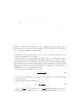
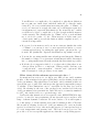
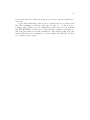
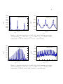
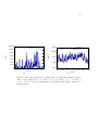
Figure 1: Schematic representation of the computed ka (νi ) spectrum, and of
the maximal error made when considering a linear variation ka∗ (ν) between
two consecutive computed result points.
be taken as ka,l (ν), for every value ν ∈ [νmin , νmax ], with a total relative error
over ka (ν) that will be lower than 1 .
The second accuracy constraint (2 ) will be used for optimizing the spectral discretization: schematically, narrowband intervals [νmin , νmax ] will be
discretized in such a way that line centers are well described. Discretization
steps will take greater values in line wings. The computation of the spectral
grid uses a tabulation of the Lorentz and Voigt functions. The method is
explained below for a Lorentz line profile.
For an isolated Lorentz line, we have:
fL =
γL2
γL
+ (ν − νc )2
(2)
with γL the Lorentz line width, and νc = ν0 +δ.P the (corrected) wavenumber at line center.
This function can be written as:
fL =
1
1
γL 1 + x2
(3)
1
c
with x = ν−ν
. Next, function f (x) = 1+x
2 has been tabulated in order to
γL
determine a series of triplets [x1 , x2 , x3 ] such that for any value x0 ∈ [x1 , x2 ],