Download Practical N°1 The random conical tilt series, using

Practical N°1
The random conical tilt series, using a simulated tilted pair
of micrographs of Lumbricus terrestris giant hemoglobin
PDF copy Practical01.pdf & annexe01.pdf
IMPMC, CNRS UMR 7590
Nicolas Boisset
and
Ricardo Aramayo
Campus Boucicaut, Université Paris 6
140 Rue de Lourmel
75015 Paris
Some informations :
For questions on this practical email to Nicolas Boisset and to Ricardo Aramayo.
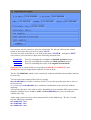
1) To use the Web software : you need to start an 8 bytes session: The JavaWed never
incorporated the Random conical tilt particle picking and lacks most of the functionnalities
required for a normal usage of display or interactive clustering, commonly used in the RCT
reconstruction scheme.
2) To get information about SPIDER operations: open this Web link :
http://www.wadsworth.org/spider_doc/spider/docs/operations_doc.html and keep it open
during the practical.
3) You will need ghostview or an equivalent program to display postcript files on your
computers. You will also need gnuplot to draw resolution curves.
3 ) For news about the SPIRE reconstruction engine, contact Bill Baxter
4) If you forgot it check the paragraph Reminder about Fourier units.
Introduction
For this practical session, we will need some files kept in "TP1.zip" (click with left button of
your mouse to download it or send me an email if you have trouble getting it), and we will
need to define a working directory and several subdirectories:
1- Create the following subdirectories : type "unzip datatp1.zip".
This should create subdirectory TP1 with six subdirectories names: micrographs, batch, doc,
images, r2d, and r3d. If you cannot download the TP1.zip from this web site, send us an
email, and we will send you the file as attched documents (size: 3.0 Mo).
4- For traveling from subdirectory to an other, you can type the following orders:
to see where you are type : "pwd"
to go to TP1 type : "cd TP1"
to go from TP1 to TP1/micrographs type : "cd micrographs"
to go from TP1/micrographs to TP1/images, type : "cd ../images"
to go from TP1/images to TP1, type : "cd .."
5- In this tutorial, we will use two softwares "spider" and "web". The spider version used
here is the latest released by Joachim Frank "VERSION: UNIX 14.16 ISSUED:
03/30/2006". For information about this latest version of spider and web contact the
Wadsworth Center for Laboratories and Research (Pr J. Franck), and visit their web site
http://www.wadsworth.org/spider_doc/spider/docs/master.html .
1. Interactive particle picking
1.1 Load the two micrographs mic001.hbl et mic002.hbl in subdirectory
TP/material:
The two micrographs are in raw 8 bytes format (rawmic001.hbl and rawmic002.hbl) in the
subdirectory micrographs. To translate then into the real*4 spider format there is a conversion
procedure. Go to the "batch" subdirectory and then type the order "spider fed/hbl b00". This
order executes a series of spider operations stored into the text file or batch file "b00.fed".
This batch file reads the 8bytes formats (rawmic001.hbl and rawmic002.hbl), and convert
them into the spider format (mic001.hbl and mic002.hbl). the same batch also rescales the
densities between values of Fmin=0 and Fmax=1 and computes images pic001.hbl and
pic002.hbl, which are the reduced versions by a factor of 2 of the original micrographs.
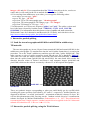
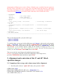
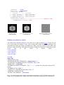
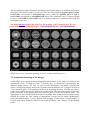
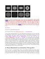
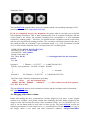
mic001.hbl and
mic002.hbl
These are synthetic images corresponding to what you could ideally get by cryoEM while
recording the same specimen field tilted by 45° and O°, respectively. Isolated particles are
disposed in different - so called "preferential" - orientations within the vitreous ice layer. We
will use this phenomenon while carrying out the "random conical tilt series" reconstruction
scheme developed by Michael Radermacher (Radermacher et al., 1987, Three-dimensional
reconstruction from a single-exposure, random conical tilt series applied to the 50 S ribosomal
subunit of Escherichia coli. J. Microsc. 146:113-136).
1.2 Interactive particle picking, using the Web Software
You must be in a 8_byte session in your linux machine to run the web software !!! This
can be a problem depending the machine you use. you can try to use Web24 in a 24_byte
session, but the background color of menus make this program unsuable.
Start the web software typing : "web hbl &" (by default the program is looking for files
*.DAT. You will have to change the default suffix by "*.hbl").
In the menu "Commands", select option "Tilted particles".
The program asks the name of the (untilted image). change in the upper window
"../TP/micrographs/*.DAT" by "../TP/micrographs/*.hbl" and click on option "filter". The list
of images with the suffix "hbl" will appear in the window. Then, click on "pic002.hbl" then
on "OK".
Then it asks for the name of the (tilted image). click on "pic001.hbl" then on "OK".
Then the program asks for a number that will be attributed to all results document files (Doc
file number). type : "001"
then the reduction factor applied to the digitized micrograhs (Reduction factor), here type "2",
then click on "Accept".
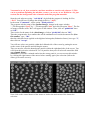
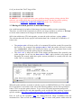
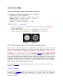
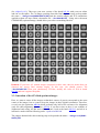
You will now select one particle within the left-hand side of the screen by putting the arrow
on the center of the particle and clicking the mouse.
Then you need to select the homologous particle within the right-hand side of the screen. You
will repeat this pairwise selection for 5 to 10 particles that you will select all around the field
(see example below):
(Remark: if you make a mistake and select the wrong particle, you can correct this mistake
by clicking the right button of the mouse before starting again your selection (follow the
orders given on the screen)).
Now click on the central button of the mouse to look at the main menu of the interactive
selection :
Click on the first option "Fit angles"
The program will ask which of your selected particle will be used as the "origin" for calculs
(Key number for origin), type "1" for instance.
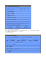
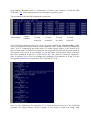
A new menu appears :
Click successively on options "Determine theta", "Fit angles", and "Save angles".
The new Theta value appears in the menu:
(normally Theta is close to 48° and phi & gamma are close to 0. see below).
Click once on "CANCEL" to shut the menu Fit angles.
Then in the main menu click on "ACCEPT" to resume the interactive particle picking.
From now on, the program knows the first estimation of respective orientations of both
micrographs, and it can help you for the pairwise particle picking. (This is not the case in this
Web version) Hence, once you will pick the tilted-specimen particle in the left-hand side of
the screen, the cursor will automatically appear on the right-hand side of the screen on the
corresponding untilted-specimen image. You might have to correct slightly the position
before clicking on the center of this second particle, but that's all . For this tutorial, you will
need to select all the particles present in your screen before going any further. Normally, you
should get 76 pairs of particles (otherwise you missed some).
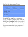
You can now restart a more accurate estimation of the (Euler angles) respective orientations
of the two micrographs now that you have all the coordinates of the particles to rely on, for
fitting of phi, theta and gamma tilt angles. Therefore, you click once on the central button of
the mouse to get the main menu, then you click on the option "Fit angles" etc... (see as above).
Finally, you will get values close to the ones shown below.
You can now stop the interactive selection of particles. For this you click one the central
button of the mouse then you click on option "STOP".
To come out of the web software, you click on the menu "SYSTEM", and option "EXIT".
All results of your selection are kept in the following document files :
dcu001.hbl
dct001.hbl
dcb001.hbl
Doc file containing the coordinates of untilted-specimen images
Doc file containing the coordinates of tilted-specimen images
Doc file containing the results of the angular determination
(Remark: Due to a bug in Web it is most likely dcu001.DAT, dct001.DAT, and
dcb001.DAT that you might obtain with this version of Web)
The doc file dft001.hbl, which is also created only contains calculation intermediates and can
be removed).
You can look at the content of these files by typing:
more dcu001.hbl (to visualize screen by screen. You need to press the space bar to move to
the next screen).
or you can type cat dcu001.hbl (for a continuous visualization of the whole file without
stopping)
You can also edit these files with an editor, depending on your machine different text editors
might be available (try vi or vim or nedit, or kate dcu001.hbl (here you can modify the
contain of the file).
At this stage you need to move these document files to the subdirectory TP1/doc. For this,
type the following commands :
mv dcu001.hbl ../doc/.
mv dct001.hbl ../doc/.
mv dcb001.hbl ../doc/.
Or if you dected the "DAT" bug in Web
mv dcu001.DAT ../doc/dcu001.hbl
mv dcu001.DAT ../doc/dcu001.hbl
mv dcu001.DAT ../doc/dcu001.hbl
WARNING ! If you would encounter some problem during particle picking with the Web
software, you could still do the rest of the tutorial, because I already put particle picking
document files (dcu001.hbl dct001.hbl dcb001.hbl) in the "doc" subdirectory.
1.3 Boxing of isolated particles in individual images
One could interactively window all the images, but that would be too time consuming.
Therefore, we will first do it interactively just for one image and then we will use a "do loop"
to do the same treatment to all images in automatic mode (or batch mode).
Still in the subdirectory TP1/micrographs, you start the spider software, typing: spider
The software then asks for the project code and the data code. In both cases it should be a 3
letters code.
•
•
The project code will be the suffix of a command file and the results file opened for
this session. For example if the project code is "fed" the spider will open a results
file "results.fed.0" which will contain the history of all the treatments done in this
session (until you stop the spider using the command EN).
The data code is simply the suffix of the images and document files opened by the
spider program. In our case the data code is "hbl", and by default every image and
document file treated within this spider session (modified or created) will have the
suffix "hbl" (ex: mic001.hbl).
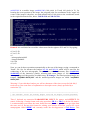
When the spider software is started, it asks the user for an OPERATION to do. The complete
list of operations is accessible on the web at the following address, but the first operation to
learn is "EN" to stop the spider software. To get a list of all spider operations and specific
explanation on what they do and what input they need, activate this link, and keep it open in a
specific window. http://www.wadsworth.org/spider_doc/spider/docs/operations_doc.html
Here we will use the operation "UD" for reading back the image coordinates from the
document files. Then we will use the operation "WI" to extract each particle within 100x100
pixel images. (Remark: pixel is a contraction of "picture" and "element"). Check the links
"UD" and "WI" in the spider manual to see how these operations work.
The document file dcu001.hbl contains the coordinates:
line Number
image
Number
X coord
Y coord
X coord
Y coord
in mic002
in mic002
in pic442
in pic442
To read back the document files, you will use registers (marked Xn, with 10<n<999), which
allow to temporarily keep in memory some numerical values. In the following example the
order "X10=1." temporarily stores the value of 1 in this register. Hence, if one answers X10
the next time spider will ask for an operation, the program will read back the value stored in
X10 and put it on screen. In our example, we use this mean with operation UD to read back
the values contained in line No.1 of file dcu001.hbl. The values are stored in consecutive
order in registers X11 to X16, for example the coordinates of the particles in X and Y on the
micrograph mic002.hbl are respectively X12=568 and X13=288.
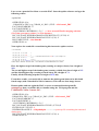
Now for the windowing, the operation WI is used and need answers to the following
questions (see figure below). In this example, if one wants to extract an image from
mic002.hbl in a smaller image unt00001.hbl (100 pixels in X and 100 pixels in Y), for
locating the exact position of the image, the programs asks for coordinates of the "upper left
corner of the images" (therefore, we must subtract half of 100 pixles to the coordinates stored
in the original document files, hence: 568-50=518 and 288-50=238.
Remark: we could also have used the values stored in the registers X12 and X13 by typing :
x12=x12-50.
x13=x13-50.
wi
../micrographs/mic002
../images/unt00001
100 ,100
x12,x13
Now, we can do these operations automatically to the rest of the images, using a command or
"batch" file. See for instance the batches b01.fed and b02.fed which will be used for the
windowing of the two micrographs. These batches read the document files (dcu001.hbl
dct001.hbl) of the interactive particle selection and create images of 100 x 100 pixels
corresponding to all the particles in subdirectory TP1/images. The tilted-specimen images are
termed "tilt[00001-00076].hbl" and the untilted-specimen images are called "unt[0000100076].hbl".
Warning ! if you edit these batches you will see that most of the time (except for b00.fed), I
took care to write some lines of explanation or descriptive note (always preceded by a
semicolon ";").
;------------------------------------------------------------------------!
; b01.fed/hbl: batch for boxing images from the 45 degree tilted specimen:
;------------------------------------------------------------------------!
Then, I declared my numerical PARAMETERS, INPUT file names, and OUTPUT file
names, following a certain format, and using operations FR L or FR G to declare file names.
I recommand that you follow the same format because (1) it is a good habit to get right from
the start, and (2) because this format for editing your batches will allow you to use a new
metaprogram called SPIRE and currently under the developpement of Bill Baxter. This
metaprogram will help you to create a library of batches easy to modify from one project to
the next, and it will allow you to create your own html based note book for each image
processing experiment. For more explanation on this very interesting development, please
contact directely Bill Baxter in Joachim Frank's laboratory at the Wadsworth Center.
; PARAMETERS
x76=76
; last image number
x81=100.
; image dimension
x82=x81/2.
; 1/2 image dimension
; INPUTS:
fr l
[init_tilted_coords]../doc/dct001
; tilted image coordinates
(from WEB)
fr l
[tilted_micrograph]../micrographs/mic001
; tilted micrograph
; OUTPUTS:
fr l
[tilted_images]../images/tilt{*****x10}
; windowed, tilted images
fr l
[new_tilted_coords]../doc/dwintilt
; new tilted image
coordinates
; END BATCH HEADER
;----------------------------------------------------------------------!
Then, to start these batches, you just need to type :
> spider new/hbl b01
> spider new/hbl b02
To visualize them, you can go in this subdirectory (cd ../images), and start the web program,
typing : web hbl &. Then you go into the COMMANDS menu and chose the option
Montage. Then click on the name of the first image of the series "tilt00001.hbl" and then
click on OK. A new window appears, asking for the number of images per line (* will
automatically adjust this value to the width of the screen), but you can also specify the
number you want 10 Frames / ROW and click on ACCEPT.
Then you can do the same thing on the untilted-specimen images.
Remark: if you want to clear the screen before displaying a new images series,
go in the COMMANDS menu and choose option Clear.
2. Alignment and centration of the 0° and 45° tiltedspecimen images
2.1 Computing of the average and variance maps before alignment
•
Start the spider software "spider hbl" and try the operation "AS R"
OPERATION: AS R
INPUT FILE TEMPLATE (E.G. PIC****): ../images/unt*****
ENTER FILE NUMBERS OR SELECTION DOC. FILE NAME: 1-76
ALL, ODD-EVEN (A/O): A
AVERAGE FILE: avg001
VARIANCE FILE: var001
The list of the 76 images appears with a message of the type :
** VARIANCE COMPUTATION BASED ON 76 IMAGES
CONTAINING 10000 ELEMENTS
TOTAL VARIANCE = 2224.0 TOTAL S.D. = 47.159
VARIANCE P.P. = 0.22240 S.D. P.P. = 0.47159
AVERAGE OFFSET = 0.00000E+00
VARIANCE OF AVERAGE IMAGE = 1.1959
OPERATION: EN --> to quit spider.
•
•
•
To look at the images start the WEB software and within the menu COMMANDS
start the option image.
Click on the name of the average map "avg001.hbl" then click on OK.
Click on the name of the variance map "var001.hbl" then click on OK.
2.2 Two-dimensional alignment of the untilted-specimen images
Here, as we have different orientations of the particle in your images, we want to align our
images while restricting the influence of a reference image to a minimum. Therefore, we will
use use a "reference free" approach developed by Pawel Penczek (Penczek, P., M.
Radermacher, et J. Frank. 1992. Three-dimensional reconstruction of single particles
embedded in ice. Ultramicroscopy, 40:33-53). Operation "AP SR" takes in charge shift and
rotation alignments in an iterative mode. When no improvement is measured from one cycle
to the next the operation stops. For each cycle an output overall image is created, and an
output document file is created, which contains rotation angle and X & Y shift to apply on
each image. As this operation is "reference free", it has a random aspect in the way images are
aligned, and it can stop after different numbers of cycles from one run to the next. Therefore I
show you below how to align images in three steps.
Run the batch b03.fed by typing the following order (remark: you must be in subdirectory
random/batch).
> spider new/hbl b03
First step, batch b03.fed applies a circular mask on the untilted-specimen images and
performs the "AP SR" operation. The Unix orders "ls -l ../r2d/avs*" and "ls -l ../doc/davs*"
are included at the end of the batch to show how many cycles were necessary to get an
optimum alignment.
You can then go to the second step of the alignment and edit the batch b04.fed and if
necessary modify the value of parameter indicating the number of cycles produced in the
previous steps:
;------------------------------------------------------------------------!
; b04.fed/hbf : - check last cycle of reference free alignment with respect
;
- to horizontal and/or vertical orientation
;------------------------------------------------------------------------!
; PARAMETERS:
X61=2.
; ending cycle number in the reference free alignment of b03.fed
Here x61=2. means that AP SR operation produced 2 cycles of alignment. If you got 4 or 5
cycles, modify parameter x61 accordingly, save your new version of the batch b04.fed with
your text editor and run it with spider. As the AP SR operation is reference-free, the output
image obtained after alignment might not be in the best orientation to conveniently apply
symmetries, or just in the best orientation for pleasing our sense of esthetic (see example
below the two global average maps obtained at the end of the two alignment cycles performed
by AP SR).
In this context, the batch b04.fed applies a mirror inversion of the output image and using
auto-correlation and angular cros-correlation functions, it finds the angle alpha necessary to
align the output image to its mirror inverted couterpart. Then, depending on the overal shape
and orientation of our output image, two solutions can be applied to get a "vertical" or
"horizontal" final orientation : either applying (alpha/2)° or applying (alpha/2)+90°. To check
this, both options are computed and put into a montage spider image called
../r2d/MALIGN.hbl (see image below) . Therefore, at the end of spider batch, you can use
the Web software to display this image (submenu: COMMAND/IMAGE in the web
software).
MALIGN001.hbl
The first row of this montage shows the output file and its mirror inverted copy. The second
raw of the montage shows their respective autocorrelation functions. Finally the last two
images correspond to the two solutions of our alignment (alpha/2)° and (alpha/2)+90°.
At this stage we can decide which of the two solutions we want to apply (here it is solution 2),
and move to the next step of the alignment. Hence, we have to edit batch b05.fed and if
necessary modify the values of parameters indicating the number of cycles produced in the
previous steps:
;----------------------------------------------------------------------!
; b05.fed/hbf : - after reference free alignment and visual checking
;
- apply solution No.1 or 2. to all original files
;----------------------------------------------------------------------!
; PARAMETERS:
X61=2.
; ending reference free alignment cycle number
X10=2.
; solution choosed No.1 or No.2 for final orientation of
particles
Here x61=2. means that AP SR operation produced 2 cycles of alignment. Once more, if you
got 3, 4 or 5 cycles, modify parameter x61 accordingly. More important here, is the value you
want to give to x10. Depending on which angle you choose X10 = 1 (for alpha/2°) or X10 = 2
(for (alpha/2)+90°). Then save your new version of the batch b05.fed with your text editor
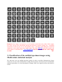
and run it with spider. The 76 images resulting from this final alignment step are kept under
the name : ../images/cenu[00001-00076].hbl and the rotation angles and X/Y translations
applied to them are kept within a document file ../doc/dalu001.hbl . Using web with menu
COMMAND, option montage, should allow you to have something like this.
Remark: If you have 90° rotated images compared to these ones, then its means that you
choosed the wrong final rotation angles. In this case you should remove file
../doc/dalu001.hbl from your subdirectory TP1/doc, modify the value of X10 in batch
b05.fed and run it again with spider.
2.3 Centration of the 45° tilted-specimen images
Here, we want to center all the images so that their centesr of gravity correspond to the exact
center of the images, but we want to keep the images in their original orientation. Therefore,
we only use the operation AP SA which performs only half of the reference free alignment
(only the shift alignment, check also AP RA if you have time as there is an example of
alignment batch using AP RA and APSA). Hence, look at the batch b06.fed, and run it in
interactive mode with the following order : spider new/hbl b06
The images obtained after this centering step are kept under the name : ../images/cent[0000100076].hbl.
Remark: these images correspond to several random conical-tilt series whose Euler angles
phi, theta, and psi were determined during the interactive particle picking (psi = azimuthal
orientation of the tilt axis in our micrographs, theta = tilt angle), and during the rotational
alignment on the untilted-specimen images (phi). The batch b07.fed reads these angles and
stores them in a document file ../doc/dang005.hbl. Run this batch with the order: spider
new/hbl
b07.
3. Classification of the untilted-specimen images using
Multivariate statistical analysis
We must now sort our untilted-specimen images in order to produce homogeneous image
classes. In our case, this could be done visually, but in practice, one must rely on an automatic
statistical procedure, as several thousands of images with a low signal-to-noise ratio must be
sorted.
3.1 Correspondence analysis
For the analysis, we want to use only the portion of the images corresponding to the particles.
In our present course we will just apply a circular mask, using operation MO, but as you
might work on all kinds of shapes, I show you below a way to create custom made masks that
will follow the outer boudaries of your particle. If you have time, you can try it, otherwise just
go further down to " Running correspondence analysis".
Custom made mask:
The first operation to compute a mask that will roughly follows the outer shape of the global
of your particle is to compute the total average map of your aligned particles. This was done
at the end of batch b06.fed, which created the map ../r2d/avgu001.hbl. From this map we will
create a binary image (containing 1. and 0. as densities), we use operation TH M, and then
operation FQ NP to smooth out and filter this binary image. Finally TH M is used once more
to create a new binary image from its smoothed out copy. (For example, look below and try to
reproduce this mask interactively to create your own mask within subdirectory TP1/r2d:
Watch out when using TH M operation as the Threshold density will change greatly the size
and shape of the output binary file.
Creation of a mask :
cd ../r2d
spider hbl
.OPERATION: TH M
.IMAGE TO BE THRESHOLDED FILE: ../r2d/avgu001
.OUTPUT FILE: scr001
.BLANK OUT (A)BOVE OR (B)ELOW THRESHOLD? (A/B): B
.THRESHOLD: 0.8 ---------------------------------> Watch out for this value !
.OPERATION: FQ NP
.INPUT FILE: scr001
.OUTPUT FILE: scr002
1 - LOW-PASS,
2 - HIGH-PASS
3 - GAUSS LOW-PASS, 4 - GAUSS HIGH-PASS
5 - FERMI LOW-PASS, 6 - FERMI HIGH-PASS
7 - BUTER LOW-PASS, 8 - BUTER HIGH-PASS
.FILTER TYPE (1-8): 3
.FILTER RADIUS: 0.08
.OPERATION: TH M
.IMAGE TO BE THRESHOLDED FILE: scr002
.OUTPUT FILE: ../r2d/mask01
.BLANK OUT (A)BOVE OR (B)ELOW THRESHOLD? (A/B): B
.THRESHOLD: 0.1 --------------------------------------------> Watch out for this value !
Depending on which Threshold values and how strongly you smooth out the first binary file,
you can expand or shrink the mask. Two operations were also developped to do the same
effects, and you can also try them. They are called DI to dilate and ER to erode any binary
map.However, they tend to form "squarish" shapes, if used intensively.
Reminder about the correspondence between Fourier units and real space
distances:
The spider software uses Fourier units which are independant of the size of the image. As
some operations will ask you some radius for filtering in Fourier space, this little paragraph
reminds you how to deal with Fourier units :
ƒ
ƒ
in reciprocal distances,
in absolute Fourier units (0 < Rf < 0.5) with Nyquist Frequency =
0.5,
ƒ
or in pixel numbers.
Lets take the image ../r2d/avgu001.hbl used to create the MSA mask. Knowing that this
images has a size of NSAM = 100 pixels and a pixel size of 3.5 Å. You can excecute a low-
pass filtering of this image at 1/35 Å-1 resolution, and a high-pass filtering at 1/25 Å-1
resolution.
NSAM = 100 (image of 100 x 100 pixels)
Ra = Radius in reciprocal Angstroems (1/Å)
PS = 3.5 A (pixel size = 3.5 Å)
Rf = Radius in Absolute Fourier units (0 < Rf < 0.5)
Rx = Radius in Fourier space with
Rp = Radius in pixels
./r2d/avgu001.hbl
Always remind these conversion rules in spider :
.OPERATION: FQ NP
.INPUT FILE: ../r2d/avgu001
.OUTPUT FILE: scr001
1 - LOW-PASS,
2 - HIGH-PASS
3 - GAUSS LOW-PASS, 4 - GAUSS HIGH-PASS
5 - FERMI LOW-PASS, 6 - FERMI HIGH-PASS
7 - BUTER LOW-PASS, 8 - BUTER HIGH-PASS
.FILTER TYPE (1-8): 5
.FILTER RADIUS: 0.1 <--------------------------------Radius in Rf
.TEMPERATURE (0=CUTOFF): 0.02
.OPERATION:
FQ NP
.INPUT FILE: ../r2d/avgu001
.OUTPUT FILE: scr003
1 - LOW-PASS,
2 - HIGH-PASS
3 - GAUSS LOW-PASS, 4 - GAUSS HIGH-PASS
5 - FERMI LOW-PASS, 6 - FERMI HIGH-PASS
7 - BUTER LOW-PASS, 8 - BUTER HIGH-PASS
.FILTER TYPE (1-8): 6
.FILTER RADIUS: 0.14 <--------------------------------Radius in Rf
.TEMPERATURE (0=CUTOFF): 0.02
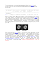
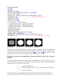
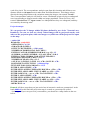
Original image
../r2d/avgu001.hbl
Low_pass filtered at 1/35 Å-1
../r2d/scr001.hbl
High-pass filtered at 1/25 Å-1
../r2d/scr003.hbl
Running correspondence analysis
The multivariate statistical analysis is now done by a single operation CA S. It will ask you
for a prefix name (for instance coran1, and it creates four output files corresponding to: the
sequential file (SEQ), the image coordinates file (IMC), the pixel coordinate file (PIX), and
the eigen values file (EIG). The output file names will then be formed by a conbinaison of the
prefix
and
of
the
suffix,
as
shown
below
:
coran1_SEQ.hbl
coran1_IMC.hbl
coran1_PIX.hbl
coran1_EIG.hbl
cd ../r2d
spider hbl
.OPERATION: CA S
.ENTER IMAGE FILE TEMPLATE: ../images/cenu*****
.ENTER FILE NUMBERS OR SLECTION DOC FILE: 1-76
.MASK FILE: ../r2d/mask01
.NUMBER OF POINTS IN MASK: 5785 <---------- (remark: here the mask contains 5785
pixels)
.NUMBER OF FACTORS : 7
.CORAN, PCA, OR SKIP ANALYSIS (C/P/S) : C
.ADDITIVE CONSTANT: 0.2
.OUTPUT FILE PREFIX~: ../r2d/coran1
Here, one could imagine that within a multi-dimensional space (with 5785 dimensions) each
image can be represented by a single point whose coordinates are the densities contained in
each of its pixels. The correspondence analysis start from this situation and defines a new
distance based on chi square metric rather than Euclidian distances. This change relates
directly the image disposition to the variations among the images, also termed "trends".
Then, correspondence analysis will look for a new coordinated system relying on orthogonal
axes corresponding to biggest trends within our image population. These new axes, also
termed "factorial axes" or "eigen vectors" are independent as they are orthogonal, and they
are sorted by decreasing order.
Projection maps:
We can project the 76 images within 2D planes defined by two of the 7 factorial axes.
Intuitively, one can see that two closely related images will be projected nearby each
other on the projection plan, while two images very different will be projected far apart
on the map.
> spider hbl
Results file: results.hbl.1
.OPERATION: CA SM
.(I)MAGE OR (P)IXEL: I
.OUTPUT FILE PREFIX~: ../r2d/coran1
.NUMBER OF HORIZONTAL PATCHES: 1
.ENTER 2 FACTOR NUMBERS FOR MAP (e.g: 1,5): 1,2
.(S)YMBOL, (A)SSIGN SYMBOL, (C)LASS, (D)OC, (I)D: S
.ENTER 1 CHAR. SYMBOL FOR ACTIVE IMAGES: o
.PREPARE POSTSCRIPT MAP? (Y/N): Y
.NUMBER OF SD OR <CR>=2.3: 3
.1=FLIP #1/ 2=FLIP #2/ 3=FLIP 1+2/ <CR>=NO FLIP: <CR>
.POSTSCRIPT OUTPUT FILE: ../r2d/map12.ps
.TEXT SIZE FOR AXIS AND DATA : 12,12
.ENTER X AXIS OFFSET: <CR>
.ENTER NEW LOWER, UPPER AXIS BOUND or <CR>: <CR>
.ENTER NEW AXIS LABEL UNITS /LABEL or <CR>: <CR>
.ENTER LABEL NO .....etc or <CR> TO CONTINUE: <CR>
.ENTER Y AXIS OFFSET: <CR>
.ENTER NEW LOWER, UPPER AXIS BOUND or <CR>: <CR>
.ENTER NEW AXIS LABEL UNITS /LABEL or <CR>: <CR>
.ENTER LABEL NO .....etc or <CR> TO CONTINUE: <CR>
.OPERATION: en
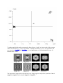
Remark: All these steps that you just carried out in interactive mode are summerized in the
batch b08.fed. In this batch the projection map is created as a postscript file called :
../r2d/map.ps. If you can open it on your machine, you should see a map similar as the one
below :
To understand which trends correspond to factorial axes 1 and 2, we keep track of the extreme
values on each axis (e.g., Axis (1) [-0.2045 : 0.2424], and Axis (2) [-0.11 : 0.12]) and we can
use operations CA SRD and CA SRA to create importance and reconstitution images for
factorial axes 1 and 2.
The importance images show which pixels vary along negative and positive portions of axis 1
(imp111 & imp112) and of axis 2 (imp121 & imp122).
The reconstitution images show how should look an original image if it would be projected at
the negative and positive edges of each axis. Here one can see that the negative part of axis 1
(rec111.hbl) corresponds to hexagonal top views, while the positive part of axis 1
(rec112.hbl) corresponds to rectangular side views. The meaning of axis 2 is more difficult
to guess (rec121.hbl et rec122.hbl), but it is clearly related to a variation concerning the
rectangular side views.
The batch b09.fed explores the same way the meaning of all 7 factorial axes. We can
look at the at the resulting montages ../r2d/MIMP001.hbl and ../r2d/MREC001.hbl.
What can you say about the meaning of axis 3 and the remaining axes ?
3.2 Automatic clustering of the images
At this stage, we are going to use the simplified representation of our image set which are the
coordinates of our 76 images on the 7 factorial axes, to characterize automatically the
different image classes. For this, we will use the Hierarchical Ascendant Classification
(HAC), which progressively merges the 76 points (corresponding to our 76 images in our new
7 axes factorial space). The merging is done in an ascending direction. First the two closest
points (most similar images) are merged in a single point. The mass and location of this new
point correspond to the global mass and center of gravity of the two original points. The
aggregation is then resumed with the nearest next points until all the points are progressively
merged in a single one. The "history of aggregation" is kept in a file called "dendrogram"
(from the greek dendros = roots). Indeed, each merging of two points is represented by a
vertical step whose height is related to the total "distances" and "masses" of the merged
points.
Lets see on a practical level how to run the HAC. Start the spider software and type the
following orders:
>spider hbl
.OPERATION: cl hc
.CORAN/PCA FILE (e.g. CORAN_01_IMC~) FILE: ../r2d/coran1_IMC
.FACTOR NUMBERS: 1-7
.FACTOR WEIGHT: 0
. CLUSTERING CRITERION (1-5): 5 <-- here we used Ward's merging criterion
(No.5) but you can try others 1 or 2 for instance.
DO YOU WANT DENDROGRAM POSTSCRIPT PLOT? (Y/T/N): N
.DO YOU WANT DENDROGRAM DOC FILE? (Y/N): Y
.DOCUMENT FILE: ../doc/dhac001
.OPERATION: en
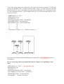
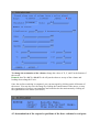
Now explore the results file created during this interactive spider session:
> cat results.hbl.4
147 135 141 18 18. 0.61
*
148 143 146 36 36. 0.75
*
----------------------------------------------------> Threshold value between 0.75 & 7.1 (for example: 3.0)
149 129 145 22 22. 7.1
****
150 147 149 40 40. 15.
*******
151 148 150 76 76. 2.03E+02 ***************************************************
NODE INDEX SENIOR JUNIOR SIZE DESCRIPTION OF THE HIERARCHY CLASSES
Here the highest step of the dendrogram (creating two major classes) has a height of
203.
The second highest step of the dendrogram (creating a third class) has a height of 15.
and the third highest step (creating a fourth class) has a height of 7.1
Finally, all the following steps have a height of 0.75 only.
From these results, you can decide to truncate the dendrogram between its third and
fourth steps (with a threshold of 3.0 for instance). This will sort four image classes.
Restart spider and run again the HAC to create a truncated dendrogram file
psdndplot.ps that you will be able to visualize using the Web program and the
COMMAND "Show Contour file".
.OPERATION: cl hc
.CORAN/PCA FILE (e.g. CORAN_01_IMC~) FILE: ../r2d/coran1_IMC
.FACTOR NUMBERS: 1-7
.FACTOR WEIGHT: 0
. CLUSTERING CRITERION (1-5): 5
.DO YOU WANT DENDROGRAM PLOT FILE? (Y/T/N):T
.ENTER PLOT CUTOFF: 3.
. DENDROGRAM FILE: ../r2d/psdndplot ------------> postcript file containing the truncated
dendrogram
.DO YOU WANT DENDROGRAM DOC FILE? (Y/N): n
.OPERATION: en
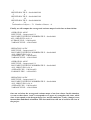
To see how many images are contained in each class, you can use operation "CL HD" and
specify the threshold value rescaled between 0 and 1. Here, you just divide the absolute
threshold value of (3.0) by the highest step value of the dendrogram (203.). Results are stored
in a new document file (here ../doc/dcount001.hbl), but you can also read then directly on the
screen (see below).
.OPERATION: x11=3/203
.OPERATION: cl hd
.Threshold (0-1): x11
.Dendrogram document FILE: ../doc/dhac001
.DOCUMENT FILE: ../doc/dcount001
OPENED DOC FILE: ../doc/dcount001.hbl
1.
18.
2.
4.
3.
18.
4.
36.
Total number of objects = 76 Number of classes = 4 .
In our case, the resulting truncated dendrogram postscript file ../r2d/psdndplot.ps looks as
shown above.
We are now going to keep in document files the list of images corresponding to each
class:
.OPERATION: x11=3/203 <-- same threshold value
.OPERATION: cl he
.Threshold: x11
.Dendrogram document FILE: ../doc/dhac001
.Enter template for selection doc: ../doc/dcla***
OPENED DOC FILE: ../doc/dcla001.hbl
Group number
Number of elements
1
18
OPENED DOC FILE: ../doc/dcla002.hbl
2
4
OPENED DOC FILE: ../doc/dcla003.hbl
3
18
OPENED DOC FILE: ../doc/dcla004.hbl
4
36
Total number of objects = 76 Number of classes = 4
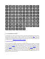
Finally, we will compute the average and variance maps of each class as shown below:
.OPERATION: AS DC
.INPUT FILE: ../images/cenu****
.DOCUMENT WITH FILE NUMBERS FILE: ../doc/dcla001
.ALL, ODD-EVEN (A/O): A
.AVERAGE FILE: ../r2d/clavg001
.VARIANCE FILE: ../r2d/clvar001
.OPERATION: AS DC
.INPUT FILE: ../images/cenu****
.DOCUMENT WITH FILE NUMBERS FILE: ../doc/dcla002
.ALL, ODD-EVEN (A/O): A
.AVERAGE FILE: ../r2d/clavg002
.VARIANCE FILE: ../r2d/clvar002
.OPERATION: AS DC
.INPUT FILE: ../images/cenu****
.DOCUMENT WITH FILE NUMBERS FILE: ../doc/dcla003
.ALL, ODD-EVEN (A/O): A
.AVERAGE FILE: ../r2d/clavg003
.VARIANCE FILE: ../r2d/clvar003
.OPERATION: AS DC
.INPUT FILE: ../images/cenu****
.DOCUMENT WITH FILE NUMBERS FILE: ../doc/dcla004
.ALL, ODD-EVEN (A/O): A
.AVERAGE FILE: ../r2d/clavg004
.VARIANCE FILE: ../r2d/clvar004
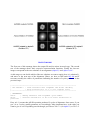
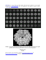
One can see below the average and variance maps of our four classes. In this situation,
we can see that classes 1 and 3 correspond to two types of rectangular side views, while
class 4 corresponds to the hexagonal top view, and the small class 2 (only 4 images) to an
intermediate undefined orientation. This last small class will not be used for the rest of
the project.
Remark : All these classification steps can be carried out automatically, using the batch
b10.fed. However, the new Web software allows now a fast computation of the truncated
dendrogram and of the corresponding average images. Therefore, the exploration of
automatic classifications is now done almost instantly ! To try this option, you need to
overcome a small bug in Web, which currently seems to open by default only images
with a ".DAT" suffix. The batch b16.fed will help you to rename the files necessary for
trying the Web interactive clustering program. Then you only need to start the program
web :
Web hbl &
Then choose Command "Dendrogram"
The program will ask for the dendrogram doc file -> ../doc/dhac001.hbl
A new window will open asking you to pick a Threshold value between 0 and 1 for truncating
the dendrogram. If you want to compute the averages corresponding to each class, you will
need to activate the option "Show Averaged images" and enter the template of the
original images subjected to this classification (in your case, you can type
"../images/cenu0001.hbl"), and click on "ACCEPT". The histogram and corresponding
average maps will instantly appear on your screen. To get a new view click on the central
button of your mouse and change the Threshold value from 0.5 to 0.05, 0.005, and finally to
0.0005. You will see that the lower you get the more smaller classes you will get. And you
can also see that if you use a very small threshold ( 0.0005) you will get several averages
looking alike, indicating that you are cutting too low and are artificially creating classes which
are in fact identical. In our case the threshold of 0.005 (if you used Ward's merging criterion)
seems the more appropriate as it distinguishes the two side views, the hexagonal and the
intermediate views into 4 classes as shown above.
4. Three-dimensional reconstruction of the particle
We have now three well defined image classes on the untilted-specimen micrograph, and we
know that their corresponding images windowed from the tilted-specimen micrograph
produce three random conical tilt series of projection of our particle. As we have now the list
of images contained in each class and we know their Euler angles (phi, theta, psi) specifying
their orientation in space. With all these informations we can compute the 3D reconstruction
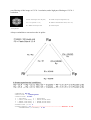
of our particle.
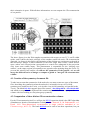
The above figure gives the Euler angular conventions with respect to axes X, Y, and Z within
spider, and it shows the basic principle of the random conical tilt-series 3D reconctruction
approach. As shown in this figure, the limitation of the tilt that one can impose to the grid in
the microscope induces a direct limitation of the Euler angle theta. Hence, within Fourier
space (where each 2D projection corresponds to a central slice orthogonal to the projection
axis) some areas remain empty. This phenomenon is responsible for the "missing cone
artifact", as the empty regions correspond to two opposite cones pointing along the Z axis. To
prevent this missing cone artifact, we will use the symmetries of the particle, and we will
merge the different series of images to compute a global or "merged" 3D reconstruction
volume.
4.1 Creation of the symmetry document file
To take into account the symmetries of the molecule, one must create two types of document
files, describing the symmetries when the molecule is oriented in its top view (6-fold
symmetry axis parallel to the Z axis), or in its side view (6-fold symmetry axis parallel to the
Y axis). The batch b11.fed computes these files named ../doc/d6top.hbl & ../doc/d6side.hbl
and which correspond to the different Euler rotation angles which allow to superpose the
volume with its according to a D6 point-group symmetry.
4.2 Computation of three distinct 3D reconstruction volumes
For the 3D reconstruction itself, we will use the BP RP operation which is the SIRT algorithm
(Simultaneous Iterative Reconstruction Technique) (See Penczek, P., M. Radermacher, et J.
Frank. 1992. Three-dimensional reconstruction of single particles embedded in ice.
Ultramicroscopy, 40:33-53). The batch b12.fed can be used to run these operations, but you
should at least use once the BP RP operation in the interactive mode to better understand its
function and adjust the values of some parameters. Here three volumes corresponding to
classes number 1, 3, and 4 will be computed. They are termed ../r3d/vcla001.hbl,
../r3d/vcla003.hbl, et ../r3d/vcla004.hbl.
Remark: If BP RP is too slow on your machine, or if you are on a hurry, check the end of
batch b12.fed , where the use of operation "BP 3F" is described.
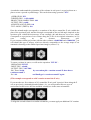
These volumes can be visually checked using the Web software :
COMMAND "Image" can visualize a series of 2D slices within the volume along axes X, Y,
or Z.
COMMAND "Surface" computes a surface rendering of the volume corresponding to a
specific threshold value, and in a specific orientation. The user manual of web can be checked
to better understand how these operations work, but we will see here a quick preview.
Start the web software typing : "web hbl &"
Within the menu "Commands", select option "Surface".
The program will ask for the name of the name of the volume. Click on "vcla001.hbl" then on
"OK".
A new window then pops up (see below). Chose the following options :
XYZ
Scale = 4.0
You can also change the threshold value for the surface rendering "Threshold" This value
must remain between the actual minimum and maximum densities of the volume (reminded in
the line "range :" at the top of the page (here minimum = -0.009736 & maximum =
0.047027).
To change the orientation of the volume, change the values of X, Y, and Z at the bottom of
the screen.
Remark: here X = 90, Y = 90, & Z = 0 will put the observer on top of the volume and
looking down along the Z axis.
Once the surface rendering is computed, you can start again by clicking on the left button of
the mouse. You can also save the image by clicking the central button of the mouse, or stop
the computation of surface representations and come back to the main menu by clicking on
the right button of the mouse (see below).
4.3 determination of the respective positions of the three volumes in real space
A method to understand the orientation of the volumes in real space is to project them on a
plan to create a pseudo cryoEM image. This can be done using operation "PJ 3".
.OPERATION: PJ 3
.THREED FILE: ../r3d/vcla001
.PROJECTION SAMPLE DIM.: 100
.OUTPUT FILE: scr001
.AZIMUTH ANGLE (PHI): 0.0
.TILT ANGLE (THETA): 0.0
Here the azimuth angle corresponds to a rotation of the object around the Z axis (within the
plan of the specimen grid), and the tilt angle corresponds to the real tilt angle imposed on the
specimen grid within the microscope. In our example, phi and theta are set to zero, which
corresponds to a projection of our volume along the Z axis in its original orientation, as if it
were
resting
on
the
electron
microscope
grid.
If you compute similar projections with the other volumes vcla003.hbl and vcla004.hbl, you
will obtain this type of images, which are directly comparable to the average maps of our
automatic clustering on the untilted-specimen images (section 3.2).
To rotate a volume in space, we will use the operation "RT 3D" :
.OPERATION: RT 3D
.INPUT FILE: vcla001
.OUTPUT FILE: VOUT001
.Phi, Theta: 90.,90.
by convention phi = rotation around Z, then theta =
rotation around Y
.Psi: -90.
and finally psi = rotation around Z again.
(This example corresponds to a 90° rotation around the X axis)
If you turn the two first volumes of 90° around the X axis, and "reproject" them along the Z
axis as previously (Azimuth/phi and tilt/theta = 0), you will produce this new type of
projections. In this series, the first and third volumes are in the same orientations.
To align the second volume in a similar orientation, you must apply an additional 30° rotation
around the Z axis.
The batch b13.fed computes these series of rotations and the corresponding montages of 2D
projections shown above (mpro[001-003].hbl).
If you are completely lost in your alignment, the spider software can help you to find the
best matching orientation. This is done stochastically from an original orientation, and the
result found is not always the optimal orientation but corresponds to a local minimum
searched by random jumps... Therefore, you should run this orientation search several times
and always using different starting positions. The correlation coefficient printed at the end of
the search provides an evaluation of the orientation search (e.g., if the correlation is around
0.3 it is really a bad orientation, but if it is larger than 0.85 it is rather good).
.OPERATION: OR 3Q X11,X12,X13,X14
.Reference 3D FILE: ../r3d/vcla004
.Second FILE: ../r3d/vcla001
.Radius of the mask: 41.
.Phi, Theta: 90.,90.
search
.Psi: -90.
<--- Starting position for the orientation
Iteration #
1 Distance = 0.5315237 r= 0.4684763064118211
FUNIQ - new parameters 90.0000 90.0000 90.0000
!
!
!
!
<--- iterations
V
V
Iteration #
182 Distance = 0.1053701 r= 0.8946299150353252
The Euler angles found by minimization procedure
Phi,
theta,
psi and function value
90.0001 89.9993 -90.0005
0.8946275
<--- these values are stored in registers
X11, X12, X13, et X14
The batch b14.fed, starts several orientation searches and the resulting values in document
file ../doc/dalv001.hbl.
4.4 Merging of the three volume
Rather than adding the three reconstruction volumes aligned in real space, a more elegant
solution is to compute a new global volume after modifying the Euler angles assigned to the
images to take into account the results of the orientation search. As it is a delicate step, it is
safer to use the batch mode to keep track of what you do. The batch b15.fed execute the
following treatments for each image series, (1) a modification of Euler angles, (2) a copy of
the images under a new name and with consecutive numbers ../images/cent[10001-
10072].hbl, (3) a copy of the new Euler angles with consecutive numbers in a new angular
document file ../doc/dang010.hbl, and (4) computation of the global or merged volume
../r3d/vtot001.hbl.
Finally, we hope this rapid tutorial helped you in your first 3D reconstruction of a signle
particle, and we wish you good luck for your own research projects !
Friendly yours,
Nicolas.
(Please send me your comments by email at "[email protected]"or
"[email protected]" to help me improve this tutorial).