1
MRITool User’s Manual
Version 1.0, February 2000
E. Loli Piccolomini
F. Zama
Department of Mathematics
University of Bologna, Italy
G. Zanghirati
Department of Mathematics
University of Ferrara, Italy
A. R. Formiconi
S. Martini
Department of Clinic Pathofisiology
University of Florence, Italy
Supported by the 1998–2000 MURST Project
“Numerical Analysis: Methods and Mathematical Software”
Abstract
MRITool is a Matlab package for functional Magnetic Resonance Imaging
(fMRI) reconstruction. It implements different reconstruction methods and provides a quite flexible graphical interface. The work was financed by the Italian
MURST Project “Numerical Analysis: Methods and Mathematical Software”
1998–2000 (http://www.unife.it/AnNum97).
The software, developed by mathematicians in cooperation with other reserchers working at the Department of Nuclear Medicine of Careggi Hospital,
was firstly motivated by the fact that the reconstruction method available on
the Phillips MRI system at the Hospital was not completely satisfactory. In fact,
it is known in literature that this method, the Keyhole method, can produce
artifacts in the reconstructed MRI images. Our research started by investigating some alternative methods proposed in literature and the MRITool software
is the mean to analyse with the medicians the results obtained. With the toolbox it is possible to test the methods on real data sets (acquired for example
by the 1.5T wholebody Phillips system at the Careggi Hospital), as well as on
“simulated” data.
MRITool is freely available (for non commercial use only) from the URL
http://dm.unife.it/ ∼mritool.
E. Loli Piccolomini
F. Zama
Dipartimento di Matematica, Università di Bologna P.zza di Porta S. Donato,
5 - 40100 Bologna, Italy. E-mail: {piccolom,zama}@dm.unibo.it.
G. Zanghirati
Dipartimento di Matematica, Università di Ferrara via Machiavelli, 35 - 44100
Ferrara, Italy. E-mail: [email protected].
A. R. Formiconi
S. Martini
Dipartimento di Fisiopatologia Clinica, Università di Firenze viale Morgagni,
85 - 50134 Firenze, Italy. E-mail: {arf,s.martini}@dfc.unifi.it.
MRITool User’s Manual
Contents
Contents
i
1 Introduction
1
2 Installation and getting started
2.1 Getting help . . . . . . . . . . . . . . . . . . . . . . . . . . . . . .
3
4
3 MRITool overview
7
4 Using the MRITool graphical interface
4.1 Load option . . . . . . . . . . . . . . . .
4.2 Method option . . . . . . . . . . . . . .
4.3 Sessions option . . . . . . . . . . . . . .
4.4 Sections option . . . . . . . . . . . . . .
4.5 Global changes option . . . . . . . . . .
4.6 Redisplay images option . . . . . . . . .
4.7 Close images option . . . . . . . . . . .
4.8 Exit option . . . . . . . . . . . . . . . .
4.9 A typical reconstruction session . . . . .
Bibliography
.
.
.
.
.
.
.
.
.
.
.
.
.
.
.
.
.
.
.
.
.
.
.
.
.
.
.
.
.
.
.
.
.
.
.
.
.
.
.
.
.
.
.
.
.
.
.
.
.
.
.
.
.
.
.
.
.
.
.
.
.
.
.
.
.
.
.
.
.
.
.
.
.
.
.
.
.
.
.
.
.
.
.
.
.
.
.
.
.
.
.
.
.
.
.
.
.
.
.
.
.
.
.
.
.
.
.
.
.
.
.
.
.
.
.
.
.
.
.
.
.
.
.
.
.
.
9
9
11
13
14
15
16
17
17
17
23
MRITool User’s Manual
Chapter 1
Introduction
This software was developed during the work made for the Italian MURST
project “Numerical Analysis: Methods and Mathematical Software”, 1998–2000
(http://www.unife.it/AnNum97). One of the main results obtained with this
work is that an interdisciplinary collaboration between medicians, physicians,
engeneers and mathematicians has started on an interesting research topic.
The problem considered concerns functional Magnetic Resonance Imaging
(fMRI). The work was mainly motivated by the fact that the reconstruction
method available on the commercial systems is not completely satisfactory. The
aim of our work is to study alternative numerical methods for fMR images
reconstruction from the acquired data in the Fourier space [1, 2, 4, 3].
The final product of our work is a Matlab software package that provides a
graphical interface, some reconstruction methods alternative to the Keyhole and
few instruments for the images visualization. The package is available from the
URL http://dm.unife.it/ ∼mritool. The reconstructed images can then be used
for an “a posteriori” analysis that can be executed with the existing instruments
and software.
The toolbox is constituted of Matlab programs and functions. We choose the
Matlab environment for its easy use of numerical and graphical instruments and
for its large diffusion. In the last years some software packages have been produced to create virtual graphical environments for functional neuroimages such
as Positron Emission Tomography (PET or SPECT) and fMRI: V3, produced
by the Liang’s group and written in C language (http://mri.beckman.uiuc.edu),
Lyngby, a Matlab fMRI analysis toolbox (http://hendrix.imm.dtu.dk/software)
written at the Thor Center for Neuroinformatics of the Technical University of
Denmark, and the fMRI analysis package by Pawel Skudlarski (http://mri.med.
yale.edu), from the Division of Imaging Sciences Diagnostic Radiologies of the
Yale University. However, while the former does not provide a graphical interface and it does not enable the use of different regularization methods, the latters
perform the analysis of reconstructed images without implementing methods for
the images reconstruction.
The key is that PET and fMRI probes in vivo patterns of activity in the
human brain. Anything short of an interactive real-time display will not fully be
able to represent the richness of these spatio-temporal phenomena. Virtual environments play a fundamental role in mediating the dialogue between medicians,
engineers and physicists.
2
Introduction
Further details and deeper treatement of the subject, together with a larger
bibliography, can be found in [5].
MRITool User’s Manual
Chapter 2
Installation and getting
started
The only software resource necessary to use MRITool is the Matlab package, version 5.2 or higher. At present, MRITool has been tested on Unix systems (DecALPHA based and SUN) and on Windows platform (WindowsNT, Windows95
and Windows98). The source files are the same for all the platforms (compressed
in different forms for the different systems), while the data files for demos are
different, because they are stored in binary format (Matlab files with extension “
.mat”). The software is available at the URL http://dm.unife.it/ ∼mritool. The
installation procedure is the following:
Unix systems. Move to your favourite directory or to the Matlab’s toolbox
directory, download the source tar file mritool src.tar.gz and give the
following commands at the line prompt:
gunzip mritool src.tar.gz
tar xvf mritool src.tar
These will expand the MRITool directory tree as a child (called mritool ) of
the current directory. If you want the demo data, from the same directory
download also the data file mritool data.tar.gz and repeat on this file
the previous commands:
gunzip mritool data.tar.gz
tar xvf mritool data.tar
These commands will add the MAT-files in the files/input subdirectory
of the mritool tree. Note that if you have gtar (GNU tar) installed, you
can replace the two commands gunzip and tar xvf with the gtar xvzf
command.
Now you can remove the .tar files from your directory. If you are performing a multiuser installation, remember to adjust the permissions of
the directory tree.
Windows systems. Download the compressed source file mritool src.zip
and uncompress it with WinZip or another suitable program, using as
destination your favorite folder or the toolbox folder of your Matlab tree.
4
Getting help
After these operations you have a new subdirectory called mritool that
contains all the toolbox files. By the same way, if you want the demo
data, download the mritool data.zip file and repeat the uncompressing
operation, unsing this time as destination the subfolder files\input of the
existing mritool folder.
Start Matlab and add mritool to your Matlab path: use the path browser
or your startup.m file if you want to add it permanently, or use the command
path from the command window if you want to add it only temporarily. In
the last case, you can first move to the MRITool parent directory ad give the
command
>> path(path,fullfile(pwd,’mritool’,’’));
or use the path command with the absolute mritool path from everywhere:
>> path(path,fullfile(matlabpath,’toolbox’,’mritool’,’’));
(see the Matlab Reference manual or the on-line help for a description of the
fullfile command). Remember that in this case you will have to repeat the
procedure for any new Matlab session.
Now you are ready to use MRITool by giving the command
>> mritool
in the Matlab’s command window. This will open the graphical interface in a
full screen style, leaving the command window still opened in background so
you will be able to perform further computation during your MRITool session.
All the MRITool functionalities are available from pup-up menus and you do
not need to type anything at the command line.
A brief description of all the commands is provided in the form of comments,
through the help system in the command window, as described in the next
section, so you could also directly call the tool scripts and functions from the
Matlab prompt. However, since in this first release we still make a rather
wide use of global variables, many functions need some variables and/or arrays
already defined in the Matlab global workspace and it can be difficult to use the
functions independently from the prompt.
2.1
Getting help
MRITool help can be viewed from the graphical interface, by clicking the Help
button or by choosing the Help option from the main menu bar: this will
show you the main help window through the default hypertext browser of your
system, that you can use to read all the functions description. If you have not a
default browser configured on your system, the standard Matlab help GUI will
be opened.
From the Matlab command window, you can get help for each function from
the Matlab prompt. For example, if you want to get help for the keyhole
function, you just need to type
>> help keyhole
Installation and getting started
5
as usual in Matlab. This version does not provide the same level of detail for
all the scripts and functions, so you could experience difficulties in some cases.
This will be fixed in a next release, however all the reconstruction codes are
based on the theory described in this work.
6
Getting help
MRITool User’s Manual
Chapter 3
MRITool overview
This toolbox provides some methods for the reconstruction of a sequence of
fMRI images from the acquired data and some tools for the visualization of
the reconstructed images. Briefly, the steps for the reconstruction of a fMRI
sequence of images are:
1. choose a data set or retrieve the data saved from a previous session;
2. choose the method for the images reconstruction;
3. choose the sections to be visualized; After the reconstruction, you are
allowed to choose, in any order, which and how many sections will be
displayed and the 2D grid in which the images will appear. Once all the
images are displayed on the screen, you are allowed to move or resize
them. You can perform a set of visualization operations on the figures all
at once, as described in section 4.5. Furthermore, each image can also be
independently elaborated.
When you want to leave the tool or to change the data, you will have to
1. save the session with if you want to continue your job later;
2. close the images on the screen;
3. leave the tool.
With this version it is possible to reconstruct:
(a) a sequence of dynamic MRI images from available real data;
(b) a sequence of dynamic MRI images from your own data, acquired in the
frequency-phase space and preprocessed to meet the required input format
(see the description in section 4.1 and the example file read binary.m in
the mritool directory).
The method for the images reconstruction can be chosen between the following:
• Reduced-encoding Imaging by Generalized-series Reconstruction with one
reference image (RIGR1).
• Reduced-encoding Imaging by Generalized-series Reconstruction with two
reference images (RIGR2).
8
MRITool overview
• Keyhole.
The methods RIGR1 and RIGR2 are combined with regularization methods for the solution of ill–conditioned linear systems. For each regularization
method, some choices for the automatic computation of the regularization parameter are proposed, together with a custom setting.
Furthermore, it is possible to show or hide the figure’s toolbar, by which you
can access many other standard useful commands as saving or exporting the
image on an external file, printing, zooming, etc. (refere to the Matlab manual
or to the on-line help for more information).
MRITool User’s Manual
Chapter 4
Using the MRITool
graphical interface
MRITool provides a graphical interface based on the powerful Matlab GUI system [10, 7]. It consists of three main parts:
• a full screen frame that constitutes a workbanch for the visualization and
elaboration of the reconstructed images;
• a main menu bar at the top of the screen, which gives access to all the
available functionalities of the tool as weel as to the help system;
• a set of five push buttons at the bottom of the screen, to facilitate the
use of the tool to beginners. In fact, The functions called by the five
buttons are essentially the same as those called by the menu items, but
the push buttons use a more friendly approach through successive GUI
windows, each having its own help button to briefly explain some details
of the related reconstruction step.
Some examples of the graphical interface during a work session is given in figures
4.1, 4.14 and 4.15. It can be noticed that buttons and menus are automatically
enabled/disabled depending on the current state of your work.
In the following subsections we’ll give an overview of the main features available through the main menu items.
4.1
Load option
The Load menu loads a data set to be processed. There are some demo data
sets already available from the MRITool web site as MAT-files for different
platforms, but the user can process its own data, once they are provided as
MAT-files in the correct format. This is obtained by using a suitable function
that reads the raw data acquired by the MRI device and then converts them
in a 3D array: we give below a brief description of this preprocess and we refer
the reader to the self explaining function read binary.m for a more detailed
description.
The available demo data are of two types (Fig. 4.2) and they are both acquired from a 1.5T wholebody MR Phillips system:
10
Load option
Figure 4.1: The basic MRITool graphical interface.
Figure 4.2: The Load menu from the main menu bar.
• the Simulated data item loads data constituted of one reference set and
one dynamic set, each of 256×256 samples. By considering only a reduced
set of phase samples (32 phases) from the dynamic set, we simulate the
undersampling process of the MRI system. As an exception, these data
are contained in two ASCII files;
• the Real-world data item loads four sequences of data: Brain 1, Brain 2,
Brain 3, Brain 4. They all are related to the same patient and each one
has the following characteristics:
-
KeyHole: 20%
RFOV: 70%
Scan percentage: 80%
Scan matrix: 128
Reconstruction matrix: 256
Two reference sets of 128 × 70 samples (section numbers 1 and 59);
57 dynamic sets of 128 × 19 samples (section numbers 2–58).
Using the MRITool graphical interface
11
Finally, with the New data option (Fig. 4.3) it is possible to process other data
sets. As mentioned, a preprocessing computation must be done in order to create
appropriate MAT-files necessary for the reconstruction with MRITool: two of
them are required, i.e. the one for the initial (baseline) reference data set and
the one for the dynamic sets; the third file, for the final (active) reference set,
can be omitted and in this case you will have not access to RIGR2 reconstruction
methods. The format for the contents of the three files is the following:
Figure 4.3: The window appearing for the loading of new data.
Initial reference image: this file must contain the baseline reference data set.
It must be stored in a matrix of size N × M , where N is the number of
frequency samples and M is the number of phase samples.
Dynamic images: this file must contain the dynamic data acquired at time
instants t1 , . . . , tQ . The data must be stored in a N ×Nm ×Q array, where
N is the number of frequency samples and Nm is the reduced number of
phase samples acquiresd at each time instant tj , j = 1, . . . , Q.
Final reference image: this file, if present, must contain the active reference
data set. It must be stored in a matrix of size N × M , where N is the
number of frequency samples and M is the number of phase samples.
4.2
Method option
With the Method menu you can choose a reconstruction method for the sequence of fMRI images. The available choices are the following:
1. Keyhole: loads the Keyhole method [5, section 1.4];
2. RIGR One Ref.:loads the Reduced-encoding Imaging by Generalized series
Reconstruction method with one reference image [5, section 1.5];
12
Method option
3. RIGR Two Refs.: loads the RIGR method with two reference images [5,
section 1.6].
Both the RIGR1 and the RIGR2 methods require a regularization method for
the solution of the hermitian and positive semidefinite linear systems, as described in section [5, section 1.7].
In this version of the tool, three regularization methods are implemented,
each one having a set of rules for the choice of the “optimal” regularization
parameter:
1. TSVD (Fig. 4.4) starts the truncated singular values decomposition method
for regularization. The possible choices for the computation of the regularization parameter are:
• GCV: generalized cross validation method [9]. This method is quite
accurate but it needs long time for the execution;
• Customize: you introduce a regularization parameter by typing a
custom value. The value must be an integer in the interval [1, Nm ],
where Nm is the number of acquired phase samples for the dynamic
sets. The default value is Nm .
We plan to add the L–curve criterion for this method in the next release.
Figure 4.4: The TSVD menu from the menu bar.
2. Lavrent’yev (Fig. 4.5) starts the Lavrent’yev regularization method. The
related regularization parameter can be computed by using one of the
following approaches:
• L-Curve: it uses the L–curve method [6, 8] which is quite accurate,
but it needs long time for the execution;
• GCV: it uses the generalized cross validation method;
• Customize: you introduce a regularization parameter by typing a
custom value. The value must be a positive number: the default is
0.1.
3. CG-type starts one of the four implemented conjugate gradient type regularization methods described in [5, section 1.7] (Fig. 4.6):
Using the MRITool graphical interface
13
Figure 4.5: The Lavrent’yev menu from the menu bar.
(a) CG is the standard conjugate gradient method applied to the linear
system;
(b) MR is the minimum residual method applied to the linear system;
(c) CGNE is the conjugate gradient method applied to the standard
normal equations;
(d) CGME is the minimum residual method applied to the normal equations of the second kind.
For each of the CG-type methods four rules for the computation of the
regularization parameter are available (stopping rules in this case):
• Heuristic 1: is a criterion proposed by Hanke, based on the behaviour
of the Ritz polynomials (one of the rules R1, R2, R3, R4 in [5, section
1.7]);
• Heuristic 2: heuristic criterion based on the residuals behaviour (rule
R5 in [5, section 1.7]);
• Heuristic 3: heuristic criterion based on the residuals behaviour (rule
R6 in [5, section 1.7]);
• Customize: you introduce a regularization parameter by typing a
custom value. The value must be a positive number in the interval
[1, Nm ], where Nm is the number of phase samples acquired for the
dynamic images. The default value is 5.
4.3
Sessions option
With this item you can save your work during a MRITool session and reload it
when necessary. When at least one work session is saved (as a MAT-file), you
can load or delete the related file. The available submenu are (Fig.4.7):
1. Save: it allows to save in a MAT-file the main MRITool variables, arrays
and structures from the Matlab workspace, in order to restart later from
the same situation. A mask appears where you can type the filename;
14
Global changes option
Figure 4.6: The conjugate gradient type menu from the menu bar.
2. Load: it loads in the Matlab workspace a previously saved work session.
The current Matlab workspace is substituted by the loaded workspace and
the saved state is completely retrieved (Fig. 4.8);
3. Delete: it allows the deletion of a previously saved file.
Figure 4.7: The Sessions menu from the menu bar.
4.4
Sections option
From this menu item a mask appears as in Fig. 4.9, containing a 2D grid that
shows you how many images can be represented on the screen and how they
can be positioned. The number of images that can be displayed depends on the
screen resolution as well as on the image size. You can select with the mouse how
many images you want to view, then a new mask appears (Fig. 4.10) where you
can choose, by clicking with the mouse, which sections you want to be displayed
(each section is identified by the number of its position in the sequence).With
the OK button the visualization process starts; it can take a little, expecially if
you have an high resolution screen and you select a large number of sections to
display, or if you are working on a remote system.
Using the MRITool graphical interface
15
Figure 4.8: The window for loading a previously saved work session.
4.5
Global changes option
Through menu allows you to control the visualization properties of all the images
on the screen. Available submenus are:
1. Image Menubar: switch on/off the figure’s menubar;
2. Colormap: changes the colormap (Fig. 4.11). In this release only standard
colormaps are available;
3. Sort Images: allows the sorting in ascending/descending order with respect to the section number, together with a “last-operation” undo (Fig. 4.13);
4. Reset to default: restore the default situation by redisplaying the images
in their initial state. Menubars and visualization mode are taken from the
current setting;
5. Visualization mode: this property affects the images aspect with respect
to axis scaling and figure size. Available choices are:
• Maintain the aspect ratio: the images are displayed by keeping the
proprtion between horizontal and veritcal size as in the corresponding
matrix;
• Fill all figure windows: the images are displayed filling all the available figure’s area. In this case the appareance can be distorted, but
the zoom capabilities (available from the figure’s menubar) are improved;
16
Close images option
Figure 4.9: The mask appearing when choosing the Sections menu from the
menu bar.
6. RIGR2 images: this submenu is available only for RIGR2 recontructions
and allows you to choose from the following items:
• Show the difference images: the images representing the changes
from the baseline to the dynamic data are displayed;
• Show the completed images: the dynamic images are displayed.
Each image can even be independently modified. By clicking with the right
mouse button while the pointer is on the single image, the just described submenu appears so that the corresponding actions can be now performed on the
single image (Fig. 4.12). However, some other items appear in this context
menu:
• Dyn. Sec.: shows the current image section number in the whole sequence;
• Image Size: gives information about the displayed matrix;
• Section: allows you to change the displayed section;
• History: shows which reconstruction process was used for the current
image.
4.6
Redisplay images option
This option acts by refreshing the graphical interface: it firstly recall the MRITool background frame and then flush all the open figures on foreground.
Using the MRITool graphical interface
17
Figure 4.10: The grid for the choice of the sections.
4.7
Close images option
It closes the displayed images, but does not leave the tool. You can still access
the reconstructed images by choosing the Sections menu to redisplay them.
4.8
Exit option
Exit from MRITool. The Matlab workspace is cleared from the tool variables,
arrays and structures, but any other “entity” is left in place, so you will not
miss your own variables and computation results, apart from unfortunate name
matching.
4.9
A typical reconstruction session
We test on the Brain 1 sequence the RIGR2 method associated with the CG
regularization method stopped with Heuristic 1 criterion (see [5, section 1.7]).
The reconstruction session can proceed as follows:
1. load the Brain 1 data set with the Load button or menu, as in Fig. 4.2;
2. choose the RIGR Two Refs. reconstruction method from the Method
menu;
3. go through the CG-type option and the CG regularization method up to
the Heuristic 1 criterion option, as in Fig. 4.6;
4. when the reconstruction is completed, select the sections to be displayed
on the screen with the Sections menu, using the two masks of figg. 4.9
and 4.10. The selected sections are displayed with the default settings
(Fig. 4.14);
18
A typical reconstruction session
Figure 4.11: A possible choice from the Global changes menu: the available
colormaps.
5. you can now change some properties of all the figures with one of the
Global changes menu options. For example, in Fig. 4.15 the colormap is
globally changed to hot.
Otherwise, you can act on the single image by changing its size and/or its
properties with the figure’s menubar or with the context menus, obtained
by clicking with the right mouse button while the pointer is on the image.
As an example, in Fig. 4.16 some characteristics of the section 32 was
modified, the figure’s Menubar was added and a zoom was performed.
With the Export option from the figure’s File menu you can save the
image in one of the standard graphic formats provided by Matlab.
Moreover, from the Matlab command window you can even perform any
type of computation on the reconstructed images, by accessing them in
the images structure in the Matlab global workspace, as described in
the MRITool help. However, given the complexity of the tool code, we
discourage this practice and we strongly recommend that you make your
computation on a copy of that structure.
6. You can finally save the current status of your work session with the Save
option of the Sessions menu;
7. you can now close the figures with the Close menu (or the corresponding
push button), without leaving the tool. At this stage, you can still make
a copy of the images structure for your own computations;
8. now you can try a different reconstruction method on the same data with
the Method menu (or push button), or you can load a different data set
with the Load menu (or push button).
9. When you have done, you will exit MRITool with the Exit option.
Using the MRITool graphical interface
19
Figure 4.12: The context menu available for a single image: the Menubar option
is “ON” for that image.
20
A typical reconstruction session
Figure 4.13: A possible choice from the Global changes menu: the ordering of
the sections displayed on the screen with respect to their number.
Figure 4.14: The selected sections are displayed with the default settings.
Using the MRITool graphical interface
Figure 4.15: The colormap has been changed to hot.
Figure 4.16: Section 32 with some characteristics modified.
21
22
A typical reconstruction session
MRITool User’s Manual
Bibliography
[1] A. R. Formiconi, A. Passeri, S. Martini, A. Pupi, E. Loli Piccolomini, F. Zama, G. Zanghirati, Regularization methods for the quantification of regional cerebral blood flow with MRI, Eur. J. Nucl. Med. 25
(1998), p. 1154.
[2] A. R. Formiconi, A. Passeri, S. Martini, A. Pupi, E. Loli Piccolomini, F. Zama, G. Zanghirati, Regularization methods in dynamic
MRI reconstruction, Eur. Radiology 1, suppl. (1999), pp. s121–s122.
[3] A. R. Formiconi, E. Loli Piccolomini, S. Martini, F. Zama,
G. Zanghirati, Numerical methods and software for functional magnetic
resonance images reconstruction, in Proceedings of the Conference “Analisi
Numerica: Metodi e Software Matematico”, Jenuary 19–21, 2000, Ferrara,
Italy, Ann. Univ. Ferrara XLVI, suppl. (2000), pp. 87–102.
[4] A. R. Formiconi, E. Loli Piccolomini, G. Parigi, F. Zama,
G. Zanghirati, Regularization methods in dynamic MRI (1999), submitted.
[5] E. Loli Piccolomini, F. Zama, G. Zanghirati, A. R. Formiconi,
S. Martini, MRITool: a Matlab tool for functional Magnetic Resonance
Imaging reconstruction, Monografia n. 2, MURST Project “Numerical
Analysis: Methods and Mathematical Software”, Ferrara (2000).
[6] P. C. Hansen, Analysis of discrete ill–posed problems by means of the
L–curve, SIAM Rev. 34 (1992), pp. 561–580.
[7] P. Marchand, Graphics and GUIs with Matlab, Second edition, CRC
Press LLc, Boca Raton (1999).
[8] D. P. O’Leary, P. C. Hansen, The use of the L–curve in the regularization of discrete ill–posed problems, SIAM J. Sci. Comp. 14 (1993), pp.
1487–1503.
[9] G. Wahba, Spline models for observational data, in CBMS–NSF Regional
Conference Series in Applied Mathematics, SIAM 59 (1990).
[10] Using Matlab Graphics, version 5, The MathWorks, Inc. (1996).