Download GIDE: Graphical Image Deblurring Exploration

GIDE: Graphical Image
Deblurring Exploration
Brianna R. Cash and Dianne P. O’Leary
We explore the use of a Matlab tool called gide that allows useraided deblurring of images. gide helps practitioners restore a blurred
grayscale image using their knowledge or intuition about the true image. At the same time, it safeguards from possible bias by validating
the choice using statistical diagnostics, based on an assumption of
Gaussian added noise. gide allows practitioners (or students) to visually explore the range of statistically likely solutions resulting from
any of three regularization methods: Tikhonov, truncated SVD, and
total variation.
In medicine and in science, we often collect raw, noisy data from a scientific
instrument (MRI, CT, astronomical camera, etc.) and process (“deblur”) this
data to produce images that are useful to practitioners. These rather expensive
images are often critical in making medical or scientific decisions, so it is important that the deblurring is performed well. Intuition tells us that if we have
a blurred image, but if we know exactly how the blur occurred – by camera
motion or an imperfect lens, for example – then we should be able to recover
the deblurred image. This is not true, though, because in practice the recorded
image has added noise, and deblurring a noisy image is an ill-posed problem.
Very small changes in the blurred image can cause very large changes in the
recovered image.
To overcome this unavoidable difficulty, regularization methods are used to
stabilize the problem [3]. These methods add an extra constraint to the recovered image to lessen the effects of noise. For example, the commonly used
Tikhonov regularization constrains the sum of the squared values in the image
to be a particular value, set by choice of a regularization parameter that we will
call γ. But then we still have the problem of choosing γ. Other regularization
methods approximate the blurring operator by a simpler one (truncated singular
value decomposition (TSVD) regularization), or limit the total variation (TV)
of the solution. Including these constraints makes the problem well-posed, and
1
2
thus the new problem has a well-determined solution that we hope is near the
true solution of the original problem. But all of these methods require choosing
a parameter γ.
So, restoring a blurred image requires choice of a regularization method
and associated parameter. Different choices can lead to a very wide variety of
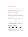
reconstructed images, as shown in Figure 1.
Practitioners faced with these choices might favor results biased by what they
expect to see and thereby introduce image artifacts or miss true image features.
This is demonstrated in Figure 2. The practitioner might not expect the moon
to have train tracks and may favor a reconstruction like the reconstructed image
in the center of the figure, where that information is lost.
Choosing an appropriate regularization method and parameter for a given
problem is difficult, relying on properties of the particular problem and knowledge of the application area. Practitioners often have invaluable experience
that is crucial in finding a good approximate solution, but too much reliance on
intuition can lead them to see what they expect to see, rather than the true solution. When possible, any candidate reconstruction should be validated using
statistical analysis.
To avoid bias, we developed a methodology for method choice and parameter
selection that uses three statistical diagnostics to validate solutions, under the
assumption of Gaussian additive noise in a blurred grayscale image.
We present a methodology and software with a graphical user interface (gui)
that can be used by practitioners to choose an appropriate regularization method
and associated parameter while reducing the bias that can be introduced by
choosing based on seeing a visually appealing reconstruction. We give practitioners the ability to compare regularization methods by showing the resulting
image and results of statistical tests of plausibility for each method and parameter they choose. We packaged the methodology into Matlab software called
gide, Graphical Image Deblurring Exploration, including a user-friendly graphical user interface (gui). The software was built upon James Nagy’s RestoreTools package [6]. It allows practitioners (or students) to visually explore the
range of statistically likely solutions resulting from any of three regularization
methods: Tikhonov, truncated SVD, and total variation.
An earlier case study [7] focussed on the mathematics of image deblurring,
and it might be useful to refer to the discussion and software (https://www.
cs.umd.edu/users/oleary/SCCS/cs_deblur/index.html) given there for an
alternate perspective. Standard textbooks [3, 4, 5, 10] might also be useful.
In this case study, we explore the use of gide. Further information about
gide can be found in the user’s manual [1] that can be downloaded with the
software from http://www.cs.umd.edu/users/oleary/software.
A Brief Overview of gide
Our proof-of-concept software package gide (Graphical Image Deblurring Exploration) was built in Matlab using the RestoreTools package [6]. Figure 3
3
Figure 1: Restorations of the 256 × 256 blurred satellite image provided in
RestoreTools [6] with signal-to-noise ratio SNR=9 and parameter γ chosen standard automatic parameter selection methods discussed below. This
indicates the wide variety of results that can be produced by regularization
methods.
Figure 2: Left: Blurred Image, Center: Deblurred Image, Right: True Image
which has “train tracks”. Without knowledge that the true image has “train
tracks” one might accept the deblurred result without realizing that important
information has been lost.
4
shows a screen shot of the interface. In this section we focus on how to install
gide and get it running on a sample problem.
ACTIVITY 1 Download the gide software from http: // www. cs. umd. edu/
users/ oleary/ software .
Then download RestoreTools from http: // www. mathcs. emory. edu/
~ nagy/ RestoreTools/ and follow the installation instructions.
Edit the gide file startGIDE.m to set path to RestoreTools and path to GIDE
to the complete directory names where you have stored these two packages.
Typing startGIDE into Matlab should bring up the gui.
The gui is easy to use. After typing startGIDE:
• A user can either provide a blurred image or choose from samples that we
provide.
• Similarly, a user either provides a blurring matrix or chooses the default
boxcar or Gaussian blurs.
The blurring matrix titled “Boxcar” is an example where the nonzero
entries of the point spread function (PSF) are given by


1 1 1
1
1 1 1 .
9
1 1 1
The entries in the PSF give the weights used in blurring. The middle entry
corresponds to the true value, and the other eight entries correspond to
the neighboring pixels. In this case, each blurred pixel value is obtained
by averaging the true value with the values of eight neighboring pixels,
creating blur.
The blurring matrix titled “Gaussian” is an example of a Gaussian
In this particular Gaussian blur, the PSF is

2
2
2
+12
+12
+12
exp(− (−1)
)
exp(− 0 2σ
exp(− 1 2σ
2
2 )
2 )
2σ
1 
(−1)2 +02
02 +02
12 +02
 exp(− 2σ2 )
exp(− 2σ2 )
exp(− 2σ2 )
2πσ 2
2
+(−1)2
02 +(−1)2
(−1)2 +(−1)2
exp(− (−1) 2σ
)
exp(−
)
exp(−
)
2
2σ 2
2σ 2
blur.


,
and σ = 0.7. Just as in the boxcar blur, each blurred pixel value is an
average of pixel values in a 3 × 3 neighborhood of the true pixel, but in
this case it is a weighted average. The numerators in the exponentials
compute the squared distance from the center pixel to each other pixel in
the neighborhood, so the weights fall off with distance from the true pixel.
5
• After selecting one of the regularization methods (TSVD regularization,
Tikhonov regularization, or TV regularization), clicking Compute generates a noisy blurred image and produces an initial solution based on
automatic selection of the regularization parameter γ.
• The resulting deblurred image appears, along with other information, including the results of the statistical diagnostics that we discuss later. For
each diagnostic, in addition to detailed information, either Yes or No is
displayed, indicating whether or not it is satisfied.
• The user then uses the slide bar to adjust γ. This changes the resulting image and diagnostics in real time, allowing the user to explore the
range of statistically plausible solutions. The blurred image, true image
(if available), and deblurred image are also displayed, for convenience, in
a separate figure.
ACTIVITY 2 At the top left of the gui, choose the “Cell” image, boxcar
blur, and Tikhonov regularization. Click Compute to obtain a candidate for
the deblurred image. Use the slidebar at the bottom left to see how the image
changes as γ is changed.
Note that if you repeat this process, then a different noise sample will be
generated, so results may change.
Now that we have gide installed and running, we explore its features. First
we will define the mathematical model of deblurring that allows us to choose
among the various regularization methods and γ values.
Mathematical Model of Imaging and Regularization
An image is recorded as an mv × mh collection of discrete square pixels, where
v denotes the vertical direction and h denotes horizontal. We form an m × 1
vector of pixels (m = mv mh ) by stacking the columns of an image into a single
column vector.
Then a discrete linear model of blur takes the form
Ax + = b,
(1)
where A is a (known) m × m blurring matrix, x is an (unknown) m × 1 vector
containing pixel values of the true image, is an (unknown) m×1 vector of noise
6
Figure 3: Screenshot of the gide gui. Choices made at the top left result in
the images displayed below and in the diagnostics on the right.
7
that we assume to be drawn from a normal distribution with zero mean, and b
is the (known) m × 1 blurred and noisy image data. Equation (1) is called a
discrete ill-posed problem because A is an ill-conditioned matrix approximating
an infinite-dimensional blurring operator.
In our sample problems, we assume that the true pixel values just outside
the border of the image are black and do not contribute to the blur of any pixel
in the image. If this assumption does not apply to a problem of interest to you,
consult a standard textbook (e.g., [5, Sec. 3.5]) for alternatives.
To regularize, we replace (1) by
1
min kAx − bk22 + γQ(x).
x 2
(2)
The first term ensures fidelity to the model (1), while the function Q (discussed
in the next section) is chosen to assure that the minimization problem is wellposed. The scalar parameter γ is chosen to balance these two objectives.
How do we find the blurring matrix? Consider an image of a single white
pixel surrounded by black pixels. The image resulting from blurring this image
is the PSF for that pixel. If the blur is identical at all pixels (i.e., spatially
invariant), then the blurring matrix can be constructed from a single PSF; see,
for example, [5, Sec. 3.2]. In general, the column of the blurring matrix A
corresponding to a particular pixel can be found by forming an image that
is black except for a single white pixel in that location and then blurring it.
Stacking the columns of the blurred image into a single column forms the column
of A.
For more details regarding finding the PSF and constructing the blurring
matrix, consult a textbook such as [5, Chap. 3].
Regularization Methods
gide gives the user a choice of three different regularization methods. Two
of the methods (Tikhonov and TSVD) can be easily applied once the singular
value decomposition (SVD) of A is computed. They were chosen because of
their widespread use, their effective damping of noise, and their ease of implementation. The third method, TV, is more expensive to apply, but it favors
solutions that include steep gradients (edges), typical of real images [10].
The Tikhonov regularization function is
Qtik (x) = kxk22 ,
Alternatively, in TSVD we regularize the problem by truncating A. Effectively, Qtsvd puts an infinite penalty on using any component of the SVD for
which the singular value is too small.
In TV regularization, our regularization function is the sum of the absolute
values of the components of the gradient of the image at each pixel. This
8
retains sharp edges in the image that may be obscured if, for example, the sum
of squares is used, as in Tikhonov regularization. The TV problem is a rather
difficult optimization problem.
ACTIVITY 3 Try each of the methods – Tikhonov, TSVD, and TV – on the
problem from the previous activity, the “Cell” image with boxcar blur. How
different are the computed solutions?
Initial Parameter Selection
A number of automated parameter selection methods have been developed, some
based on prior knowledge of the particular problem (distribution of noise or
errors), others based on statistical criteria. The parameters chosen by these
methods are often far from those that minimize the deviation of the computed
solution from the true solution [3]. In gide, automated parameter selection
methods are used only to find an initial parameter that the user can then change.
We choose to use the automated selection generalized cross validation (GCV)
for the SVD-based methods, since the computation can be performed efficiently.
For TV, GCV is too costly, so we use the discrepancy principle.
GCV is based on the popular leave-one-measurement-out model, checking
the reasonableness of a parameter determined from m − 1 measurements by
seeing how well the resulting model predicts the mth measurement [4, p. 95].
The idea is to choose the parameter γ that minimizes the prediction errors.
The discrepancy principle exploits the fact that we know the distribution of
the noise , so we can choose γ so that
kAxγ − bk2 = νE(kk2 ),
(3)
where E denotes expected value and ν = 2 is a safety factor [4, p. 90]. The
appropriate value of γ is computed by solving (3) using Matlab’s fzero, an
efficient root finding algorithm.
Statistical Diagnostics
We use statistical diagnostics to test the plausibility of a candidate regularization solution as a solution to the original ill-posed problem. We use the three
diagnostics proposed by Bert Rust [9] to generate a range of plausible regularization parameters. These diagnostics are based on the simple observation that
since
= b − Ax
9
is noise drawn from some statistical distribution, then
r = b − Axγ ,
where xγ is the regularized solution with regularization parameter γ, should
ideally equal and therefore be a sample from the same distribution. We use
standard statistical tests to evaluate how typical r is as a sample from the
distribution, which we assume to be normal with known variance.
To use the diagnostics, we normalize our problem so that the errors are
normally distributed with mean 0 and covariance matrix equal to the identity.
If the error is distributed as N (0, S2 ), and if S is known, then this can be done
by multiplying the blurring matrix A and the observed image b by S−1 .
We now discuss the three diagnostics shown on the right side of the gui in
Figure 3.
Residual Diagnostic 1 Since is a sample from the distribution N (0, Im ),
we know the distribution of kk22 : the sum of squares of a set of m independent
identically distributed (i.i.d.) standard normal random samples is a random
variable with a χ2 distribution. It has expected value m and variance 2m [8].
Therefore, our first diagnostic tests whether the residual norm squared, krk22 , is
within two standard deviations (i.e., within the 95% confidence interval) of the
expected value of kk22 . Therefore, we want
√
√
(4)
krk22 ∈ [m − 2 2m, m + 2 2m].
gide displays the residual norm-squared, the endpoints of the confidence interval
and a yes/no answer to whether we are within the confidence interval.
Residual Diagnostic 2 The histogram of the elements of r should look like a
bell-shaped curve. We use a χ2 goodness-of-fit test [8] which tests whether the
residual is drawn from an i.i.d standard normal distribution (null hypothesis)
by comparing it to the theoretical distribution. gide displays the histogram of
the residual and a yes/no answer to whether the p-value, used in the statistical
hypothesis test, satisfies p > 0.05. If yes, then one should accept the null
hypothesis with 95% confidence.
Residual Diagnostic 3 If we view the elements of and r as time series with
index i = 1, . . . , m then {i } forms a white noise series. We expect {ri } to also
be a white noise series. One way to assess this is to compute the cumulative
periodogram of the residual [2, Chapter 7]. We compare the computed values
with a 95% confidence interval for a white noise series. For more details, see the
gide manual [1].
Adjusting the parameter so that the diagnostics move into their “yes” ranges
produces a reconstruction that is statistically plausible. For a given problem,
though, there is no guarantee that a parameter exists that satisfies all three
diagnostics, even though the results of the tests are correlated.
10
ACTIVITY 4 Using the “Cell” image with boxcar blur, as in the previous
activity, with Tikhonov regularization, try to find a parameter that satisfies all
three of the statistical diagnostics. Repeat for the other two regularization methods (TSVD and TV), and compare the final images.
Complete the following sentence: Sliding γ to the left/right increases the
residual-norm-squared (Diagnostic 1), tends to push the distribution in Diagnostic 2 to the ???, and tends to move the red line (the cumulative periodogram)
in Diagnostic 3 to the ???.
ACTIVITY 5 Repeat these explorations with the other image, a 16 × 16 version of Matlab’s Shepp-Logan image. Then see if results are much different if
Gaussian blur is used instead of boxcar blur.
Limitations of gide
The speed of today’s computers limits the size of images for which real-time
response is reasonable in the gui.
gide is meant to be a tool for exploration. If gide runs too slowly on your
image, we suggest that you extract a small piece of the image. Using gide,
you can determine an appropriate regularization method and a statisticallyvalidated candidate parameter that can then be used for the full image. Using
this regularization parameter, the computation for the full image can be done
using RestoreTools or the TV program TVPrimDual.m.
gide is a working proof-of-concept that could be scaled to a faster computational tool by using a compiled computer language and high-performance
computing.
ACTIVITY 6 Choose “User Provided Blur” and “User Provided Image”, and
see how regularization works on the satellite example provided with GIDE. (Note
that the TV solver might be too slow to run well on this larger image.)
11
ACTIVITY 7 (Extra) The satellite example is generated in the file called
MyData.m. Modify that file to load your own image and blurring matrix into
gide. Then explore the possible reconstructions.
ACTIVITY 8 (Extra) gide could be extended in many ways. For example,
the regularization parameter could be specified directly, rather than through a
slidebar. Make this change to GIDE.m.
Conclusions
When important decisions need to be made based on deblurred images, it is
prudent to use a regularization method and parameter that can be justified on
statistical grounds. gide helps practitioners do this. The software takes advantage of the practitioner’s trained eyes while limiting bias by using statistical
diagnostics. Even without detailed knowledge of the numerical method, the user
can explore different solutions with real-time diagnostics determining whether
the solution is statistically plausible.
There has been work in automatic parameter selection, but these methods remain controversial and do not always produce reasonable results. Our
methodology is a straightforward alternative for determining an appropriate
method and parameter.
To effectively be used in real time, our methodology is currently limited to
relatively small images. That being said, the software has been proved useful in
an undergraduate course on image restoration, giving the students immediate
feedback about the effects of different regularization methods and parameter
choices.
12
Acknowledgements
This work, including the development of gide was supported by the National
Science Foundation under grant DMS 1016266.
Biographies:
Brianna Cash received her PhD degree in Applied Mathematics & Statistics
and Scientific Computing from the University of Maryland in 2014. She now
works for Northrup-Grumman.
Dianne O’Leary is a Distinguished University Professor, emerita, at the University of Maryland. Her research is in computational linear algebra and optimization, with applications to image processing, text summarization, and other
areas. https://www.cs.umd.edu/users/oleary
Bibliography
[1] Brianna R. Cash and Dianne P. O’Leary. A Guide to GIDE: A GUI
for Graphical Image Deblurring Exploration. Technical report, http://
www.cs.umd.edu/users/oleary/software, University of Maryland, College Park, Maryland, 2015.
[2] Wayne A. Fuller.
Introduction to Statistical Time Series.
Interscience, New York, N.Y., 1996.
Wiley-
[3] Per Christian Hansen. Rank-Deficient and Discrete Ill-Posed Problems.
Numerical Aspects of Linear Inversion. SIAM, Philadelphia, PA, 1998.
[4] Per Christian Hansen. Discrete Inverse Problems: Insight and Algorithms.
SIAM, Philadelphia, PA, 2010.
[5] Per Christian Hansen, James G. Nagy, and Dianne P. O’Leary. Deblurring
Images: Matrices, Spectra, and Filtering. SIAM, Philadelphia, PA, 2006.
[6] James G. Nagy. RestoreTools: An object oriented Matlab package
for image restoration, 2004. http://www.mathcs.emory.edu/~nagy/
RestoreTools/.
[7] James G. Nagy and Dianne P. O’Leary. Image deblurring: I can see clearly
now. Computing in Science and Engineering, 5(3):pp. 82–85, May/June
2003. Solution: Vol. 5, No. 4, July/August 2003, pp. 72–74.
[8] Sheldon Ross. A First Course in Probability, Sixth Edition. Prentice Hall,
Upper Saddle River, N.J., 2002.
[9] Bert W. Rust and Dianne P. O’Leary. Residual periodograms for choosing regularization parameters for ill-posed problems. Inverse Problems,
24(034005):30, 2008.
[10] Curtis R. Vogel.
Computational Methods for Inverse Problems.
SIAM, Philadelphia, PA, 2002.
13