Download User`s Guide - Chasqueweb

PIM 2.2
The Parallel Iterative Methods package for
Systems of Linear Equations
User's Guide
(Fortran 77 version)
Rudnei Dias da Cunha
Mathematics Institute and National Supercomputing Centre
Universidade Federal do Rio Grande do Sul
Brasil
Tim Hopkins
Computing Laboratory
University of Kent at Canterbury
United Kingdom
Abstract
We describe PIM (Parallel Iterative Methods), a collection of Fortran 77 routines to
solve systems of linear equations on parallel computers using iterative methods.
A number of iterative methods for symmetric and nonsymmetric systems are available, including Conjugate-Gradients (CG), Bi-Conjugate-Gradients (Bi-CG), ConjugateGradients squared (CGS), the stabilised version of Bi-Conjugate-Gradients (Bi-CGSTAB),
the restarted stabilised version of Bi-Conjugate-Gradients (RBi-CGSTAB), generalised minimal residual (GMRES), generalised conjugate residual (GCR), normal equation solvers
(CGNR and CGNE), quasi-minimal residual (QMR), transpose-free quasi-minimal residual
(TFQMR) and Chebyshev acceleration.
The PIM routines can be used with user-supplied preconditioners, and left-, right- or
symmetric-preconditioning are supported. Several stopping criteria can be chosen by the
user.
In this user's guide we present a brief overview of the iterative methods and algorithms
available. The use of PIM is introduced via examples. We also present some results obtained
with PIM concerning the selection of stopping criteria and parallel scalability. A reference
manual can be found at the end of this report with specic details of the routines and
parameters.
Contents
1 Introduction
2 An overview of the iterative methods
CG : : : : : : : : : : : : : : : : : : :
CG with eigenvalues estimation : : :
CGNR and CGNE : : : : : : : : : :
Bi-CG : : : : : : : : : : : : : : : : :
CGS : : : : : : : : : : : : : : : : : :
Bi-CGSTAB : : : : : : : : : : : : :
RBi-CGSTAB : : : : : : : : : : : : :
GMRES : : : : : : : : : : : : : : : :
GMRES with eigenvalues estimation
GCR : : : : : : : : : : : : : : : : : :
QMR : : : : : : : : : : : : : : : : :
TFQMR : : : : : : : : : : : : : : : :
Chebyshev acceleration : : : : : : :
3 Internal details of PIM
3.1
3.2
3.3
3.4
3.5
:
:
:
:
:
:
:
:
:
:
:
:
:
:
:
:
:
:
:
:
:
:
:
:
:
:
:
:
:
:
:
:
:
:
:
:
:
:
:
:
:
:
:
:
:
:
:
:
:
:
:
:
:
:
:
:
:
:
:
:
:
:
:
:
:
:
:
:
:
:
:
:
:
:
:
:
:
:
Supported architectures and environments : : : : : : :
Parallel programming model : : : : : : : : : : : : : : :
Data partitioning : : : : : : : : : : : : : : : : : : : : :
Increasing the parallel scalability of iterative methods
Stopping criteria : : : : : : : : : : : : : : : : : : : : :
4 Using PIM
:
:
:
:
:
:
:
:
:
:
:
:
:
:
:
:
:
:
:
:
:
:
:
:
:
:
:
:
:
:
:
:
:
:
:
:
:
:
:
:
:
:
:
:
:
:
:
:
:
:
:
:
:
:
:
:
:
:
:
:
:
:
:
:
:
:
:
:
:
:
:
:
4.1 Naming convention of routines : : : : : : : : : : : : : : : : :
4.2 Obtaining PIM : : : : : : : : : : : : : : : : : : : : : : : : : :
4.3 Installing PIM : : : : : : : : : : : : : : : : : : : : : : : : : :
Building the PIM core functions : : : : : : : : : : : :
Building the examples : : : : : : : : : : : : : : : : : :
Cleaning-up : : : : : : : : : : : : : : : : : : : : : : : :
Using PIM in your application : : : : : : : : : : : : :
4.4 Calling a PIM iterative method routine : : : : : : : : : : : :
4.5 External routines : : : : : : : : : : : : : : : : : : : : : : : : :
Matrix-vector product : : : : : : : : : : : : : : : : : :
Preconditioning : : : : : : : : : : : : : : : : : : : : : :
Inner-products, vector norms and global accumulation
2
:
:
:
:
:
:
:
:
:
:
:
:
:
:
:
:
:
:
:
:
:
:
:
:
:
:
:
:
:
:
:
:
:
:
:
:
:
:
:
:
:
:
:
:
:
:
:
:
:
:
:
:
:
:
:
:
:
:
:
:
:
:
:
:
:
:
:
:
:
:
:
:
:
:
:
:
:
:
:
:
:
:
:
:
:
:
:
:
:
:
:
:
:
:
:
:
:
:
:
:
:
:
:
:
:
:
:
:
:
:
:
:
:
:
:
:
:
:
:
:
:
:
:
:
:
:
:
:
:
:
:
:
:
:
:
:
:
:
:
:
:
:
:
:
:
:
:
:
:
:
:
:
:
:
:
:
:
:
:
:
:
:
:
:
:
:
:
:
:
:
:
:
:
:
:
:
:
:
:
:
:
:
:
:
:
:
:
:
:
:
:
:
:
:
:
:
:
:
:
:
:
:
:
:
:
:
:
:
:
:
:
:
:
:
:
:
:
:
:
:
:
:
:
:
:
:
:
:
:
:
:
:
:
:
:
:
:
:
:
:
:
:
:
:
:
:
:
:
:
:
:
:
:
:
:
:
:
:
:
:
:
:
:
:
:
:
:
:
:
:
:
:
:
:
:
:
:
:
:
:
:
:
:
:
:
:
:
:
:
:
:
:
:
:
:
:
:
:
:
:
:
:
:
:
:
:
:
:
:
:
:
:
:
:
:
:
:
:
:
:
:
:
:
:
:
:
:
:
:
:
5
7
7
8
9
9
10
10
10
10
11
11
11
11
12
13
13
14
14
15
16
17
17
17
18
18
19
20
21
21
22
22
23
24
Monitoring the iterations : : : : : : : : : : : : : : : : : :
4.6 Example programs : : : : : : : : : : : : : : : : : : : : : : : : : :
4.6.1 Eigenvalues estimation and Chebyshev acceleration : : : :
4.6.2 Dense storage : : : : : : : : : : : : : : : : : : : : : : : : :
4.6.3 PDE storage : : : : : : : : : : : : : : : : : : : : : : : : :
A matrix-vector product for parallel vector architectures :
4.6.4 Preconditioners : : : : : : : : : : : : : : : : : : : : : : : :
4.6.5 Results : : : : : : : : : : : : : : : : : : : : : : : : : : : :
Stopping criteria : : : : : : : : : : : : : : : : : : : : : : :
General results : : : : : : : : : : : : : : : : : : : : : : : :
Scalability : : : : : : : : : : : : : : : : : : : : : : : : : : :
5 Summary
References
A Reference manual
A.1 Description of parameters : : : : : : : : : : : : :
A.2 External routines : : : : : : : : : : : : : : : : : :
Note : : : : : : : : : : : : : : : : : : : : :
Matrix-vector product v = Au : : : : : : :
Transpose matrix-vector product v = AT u
Left preconditioning v = Qu : : : : : : : :
Right preconditioning v = Qu : : : : : : :
Parallel sum : : : : : : : : : : : : : : : :
Parallel vector norm : : : : : : : : : : : :
Monitoring routine : : : : : : : : : : : : :
A.3 PIM CG : : : : : : : : : : : : : : : : : : : : : : : :
A.4 PIM CGEV : : : : : : : : : : : : : : : : : : : : : :
A.5 PIM CGNR : : : : : : : : : : : : : : : : : : : : : :
A.6 PIM CGNE : : : : : : : : : : : : : : : : : : : : : :
A.7 PIM BICG : : : : : : : : : : : : : : : : : : : : : :
A.8 PIM CGS : : : : : : : : : : : : : : : : : : : : : : :
A.9 PIM BICGSTAB : : : : : : : : : : : : : : : : : : : :
A.10 PIM RBICGSTAB : : : : : : : : : : : : : : : : : : :
A.11 PIM RGMRES : : : : : : : : : : : : : : : : : : : : :
A.12 PIM RGMRESEV : : : : : : : : : : : : : : : : : : : :
A.13 PIM RGCR : : : : : : : : : : : : : : : : : : : : : :
A.14 PIM QMR : : : : : : : : : : : : : : : : : : : : : : :
3
:
:
:
:
:
:
:
:
:
:
:
:
:
:
:
:
:
:
:
:
:
:
:
:
:
:
:
:
:
:
:
:
:
:
:
:
:
:
:
:
:
:
:
:
:
:
:
:
:
:
:
:
:
:
:
:
:
:
:
:
:
:
:
:
:
:
:
:
:
:
:
:
:
:
:
:
:
:
:
:
:
:
:
:
:
:
:
:
:
:
:
:
:
:
:
:
:
:
:
:
:
:
:
:
:
:
:
:
:
:
:
:
:
:
:
:
:
:
:
:
:
:
:
:
:
:
:
:
:
:
:
:
:
:
:
:
:
:
:
:
:
:
:
:
:
:
:
:
:
:
:
:
:
:
:
:
:
:
:
:
:
:
:
:
:
:
:
:
:
:
:
:
:
:
:
:
:
:
:
:
:
:
:
:
:
:
:
:
:
:
:
:
:
:
:
:
:
:
:
:
:
:
:
:
:
:
:
:
:
:
:
:
:
:
:
:
:
:
:
:
:
:
:
:
:
:
:
:
:
:
:
:
:
:
:
:
:
:
:
:
:
:
:
:
:
:
:
:
:
:
:
:
:
:
:
:
:
:
:
:
:
:
:
:
:
:
:
:
:
:
:
:
:
:
:
:
:
:
:
:
:
:
:
:
:
:
:
:
:
:
:
:
:
:
:
:
:
:
:
:
:
:
:
:
:
:
:
:
:
:
:
:
:
:
:
:
:
:
:
:
:
:
:
:
:
:
:
:
:
:
:
:
:
:
:
:
:
:
:
:
:
:
:
:
:
:
:
:
:
:
:
:
:
:
:
:
:
:
:
:
:
:
:
:
:
:
:
:
:
:
:
:
:
:
:
:
:
:
:
:
:
:
:
:
:
:
:
:
:
:
:
:
:
:
:
:
:
:
:
:
:
:
:
:
:
:
:
:
:
:
:
:
:
:
:
:
:
:
:
:
:
:
:
:
:
:
:
:
:
:
:
:
:
:
:
:
:
:
:
:
:
:
:
:
:
:
:
:
:
:
:
:
:
:
:
:
:
:
:
:
:
:
:
:
:
:
:
:
:
:
:
:
:
:
:
:
:
:
:
:
:
:
:
:
:
:
:
:
:
:
:
:
:
:
:
26
27
29
30
30
34
35
36
36
36
37
37
40
44
45
47
47
47
47
47
47
48
48
48
49
51
53
55
57
59
61
63
65
67
69
71
A.15 PIM TFQMR : : :
A.16 PIM CHEBYSHEV
A.17 PIM SETPAR : :
A.18 PIM PRTPAR : :
A.19 INIT : : : : :
:
:
:
:
:
:
:
:
:
:
:
:
:
:
:
:
:
:
:
:
:
:
:
:
:
:
:
:
:
:
:
:
:
:
:
:
:
:
:
:
:
:
:
:
:
:
:
:
:
:
:
:
:
:
:
:
:
:
:
:
:
:
:
:
:
4
:
:
:
:
:
:
:
:
:
:
:
:
:
:
:
:
:
:
:
:
:
:
:
:
:
:
:
:
:
:
:
:
:
:
:
:
:
:
:
:
:
:
:
:
:
:
:
:
:
:
:
:
:
:
:
:
:
:
:
:
:
:
:
:
:
:
:
:
:
:
:
:
:
:
:
:
:
:
:
:
:
:
:
:
:
:
:
:
:
:
:
:
:
:
:
:
:
:
:
:
:
:
:
:
:
:
:
:
:
:
:
:
:
:
:
:
:
:
:
:
73
75
77
78
79
1 Introduction
The Parallel Iterative Methods (PIM) is a collection of Fortran 77 routines designed to solve
systems of linear equations (SLEs) on parallel computers using a variety of iterative methods.
PIM oers a number of iterative methods, including
Conjugate-Gradients (CG) [29],
Conjugate-Gradients for normal equations with minimisation of the residual norm
(CGNR) [35],
Conjugate-Gradients for normal equations with minimisation of the error norm (CGNE)
[11],
Bi-Conjugate-Gradients (Bi-CG) [22],
Conjugate-Gradients squared (CGS) [44],
the stabilised version of Bi-Conjugate-Gradients (Bi-CGSTAB) [46],
the restarted, stabilised version of Bi-Conjugate-Gradients (RBi-CGSTAB) [43],
the restarted, generalised minimal residual (RGMRES) [42],
the restarted, generalised conjugate residual (RGCR) [20],
the highly-parallel algorithm for the quasi-minimal residual (QMR) method, recently proposed by Bucker and Sauren [8],
the transpose-free quasi-minimal residual (TFQMR) [24] and
Chebyshev acceleration [32].
The routines allow the use of preconditioners; the user may choose to use left-, right- or
symmetric-preconditioning. Several stopping criteria are also available.
PIM was developed with two main goals
1. To allow the user complete freedom with respect to the matrix storage, access and partitioning;
2. To achieve portability across a variety of parallel architectures and programming environments.
These goals are achieved by hiding from the PIM routines the specic details concerning the
computation of the following three linear algebra operations
5
1. Matrix-vector (and transpose-matrix-vector) product
2. Preconditioning step
3. Inner-products and vector norm
Routines to compute these operations need to be provided by the user. Many vendors supply
their own, optimised linear algebra routines which the user may want to use.
A number of packages for the iterative solution of linear systems are available including
ITPACK [30] and NSPCG [38]. PIM diers from these packages in three main aspects. First,
while ITPACK and NSPCG may be used on a parallel vector supercomputer like a Cray Y-MP,
there are no versions of these packages available for distributed-memory parallel computers.
Second, there is no debugging support; this is dictated by the fact that in some multiprocessing
environments parallel I/O is not available. The third aspect is that we do not provide a collection
of preconditioners but leave the responsibility of providing the appropriate routines to the user.
In this sense, PIM has many similarities to a proposed standard for iterative linear solvers,
by Ashby and Seager [5]. In that proposal, the user supplies the matrix-vector product and
preconditioning routines. We believe that their proposed standard satises many of the needs
of the scientic community as, drawing on its concepts, we have been able to provide software
that has been used in a variety of parallel and sequential environments. PIM does not always
follow the proposal especially with respect to the format of the matrix-vector product routines
and the lack of debugging support.
Due to the openness of the design of PIM, it is also possible to use it on a sequential machine.
In this case, the user can take advantage of the BLAS [16] to compute the above operations.
This characteristic is important for testing purposes; once the user is satised that the selection
of preconditioners and stopping criteria are suitable, the computation can be accelerated by
using appropriate parallel versions of the three linear algebra operations mentioned above.
A package similar to PIM is the Simplied Linear Equation Solvers (SLES) by Gropp and
Smith [31], part of the PETSc project. In SLES the user has a number of iterative methods (CG,
CGS, Bi-CGSTAB, two variants of the transpose-free QMR, restarted GMRES, Chebyshev and
Richardson) which can be used together with built-in preconditioners and can be executed
either sequentially or in parallel. The package may be used with any data representation of
the matrix and vectors with some routines being provided to create matrices dynamically in
its internal format (a feature found on ITPACK). The user can also extend SLES in the sense
that it can provide new routines for preconditioners and iterative methods without modifying
SLES. It is also possible to debug and monitor the performance of a SLES routine.
Portability of code across dierent multiprocessor platforms is a very important issue. For
distributed-memory multiprocessor computers, a number of public-domain software libraries
have appeared, including PVM [28], TCGMSG [33], NXLIB [45], p4 [9] (the latter with support
for shared-memory programming). These libraries are available on a number of architectures
6
making it possible to port applications between dierent parallel computers with few (if any)
modications to the code being necessary. In 1993 the \Message-Passing Interface Forum", a
consortium of academia and vendors, drawing on the experiences of users of those and other
libraries, dened a standard interface for message-passing operations, called MPI [23]. Today we have available implementations of MPI built on top of other, existing libraries, like
the CHIMP/MPI library developed at the Edinburgh Parallel Computer Centre [7], and the
Unify project [10] which provides an MPI interface on top of PVM. It is expected that native
implementations will be available soon. In the previous releases of PIM (1.0 and 1.1) we had
distributed examples using PVM, TCGMSG, p4 and NXLIB; however from this release onwards
we will support only PVM, the \de-facto" standard for message-passing, and MPI.
We would like to mention two projects which we believe can be used together with PIM.
The rst is the proposed standard for a user-level sparse BLAS by Du et al. [19] and Heroux
[34]. This standard addresses the common problem of accessing and storing sparse matrices in
the context of the BLAS routines; such routines could then be called by the user in conjunction
with a PIM routine. The second is the BLACS project by Dongarra et al. [17] which provides
routines to perform distributed operations over matrices using PVM 3.1.
2 An overview of the iterative methods
How to choose an iterative method from the many available is still an open question, since any
one of these methods may solve a particular system in very few iterations while diverging on
another. In this section we provide a brief overview of the iterative methods present in PIM.
More details are available in the works of Ashby et al. [4], Saad [40][41], Nachtigal et al. [37],
Freund et al. [25][26] and Barrett et al. [6].
We introduce the following notation. CG, Bi-CG, CGS, Bi-CGSTAB, restarted GMRES,
restarted GCR and TFQMR solve a non-singular system of n linear equations of the form
Q1AQ2 x = Q1b
where Q1 and Q2 are the preconditioning matrices. For CGNR, the system solved is
Q1AT AQ2 x = Q1AT b
and for CGNE we solve the system
Q1AAT Q2x = Q1b
(1)
(2)
(3)
CG The CG method is used mainly to solve Hermitian positive-denite (HPD) systems. The
method minimises the residual in the A-norm and in nite-precision arithmetic it terminates in
at most n iterations. The method does not require the coecient matrix; only the result of a
7
matrix-vector product Au is needed. It also requires a relatively small number of vectors to be
stored per iteration since its iterates can be expressed by short, three-term vector recurrences.
With suitable preconditioners, CG can be used to solve nonsymmetric systems. Holter
et al. [36] have solved a number of problems arising from the modelling of groundwater ow
via nite-dierences discretisations of the two-dimensional diusion equation. The properties
of the model led to systems where the coecient matrix was very ill-conditioned; incomplete
factorisations and least-squares polynomial preconditioners were used to solve these systems.
Hyperbolic equations of the form
@u + @u + @u = f (x; y; t)
@t 1 @x 2 @y
have been solved with CG using a Neumann polynomial approximation to A;1 as a preconditioner [12].
CG with eigenvalues estimation An important characteristic of CG is its connection to
the Lanczos method [29] which allows us to obtain estimates of the eigenvalues of Q1AQ2
with only a little extra work per iteration. These estimates, 1 and n, are obtained from
the Lanczos tridiagonal matrix Tk whose entries are generated during the iterations of the
CG method [29, pp. 475-480, 523-524]. If we dene the matrices = diag(0; 1 ; : : : ; k;1 ),
Gk = diag(0; 1; : : : ; k;1) and
2
6
6
6
Bk = 666
6
4
1 ;2
1 ;3
1 ...
. . . ;
k
1
3
7
7
7
7
7
7
7
5
where i = jj ri jj2, ri is the residual at the i-th iteration, i = pTi Api and i = riT ri =riT;1ri;1
are generated via the CG iterations (at no extra cost), we obtain the Lanczos's matrix via the
relation
Tk = ;1BkT Gk Bk ;1
(4)
Due to the structure of the matrices Bk , and Gk , the matrix Tk can be easily updated during
the CG iterations. The general formula for Tk is
ai = (i2 i;2 + i;1)=2i;1 ; 1 = 0; i = 1; 2; : : : ; k
bi = ;i;1i+1=(i;1i ); i = 1; 2; : : : ; k ; 1
8
where ai and bi are the elements along the diagonal and subdiagonal of Tk respectively.
The strategy employed to obtain the eigenvalue estimates is based on Sturm sequences [29,
pp. 437-439]. For the matrix T2, obtained during the rst iteration of CG, the eigenvalues are
obtained directly from the quadratic equation derived from p() = det(T2 ; I ). We also set
an interval [c; d] = [1; n].
For the next iterations, we update the interval [c; d] using Gerschgorin's theorem. This is
easily accomplished since at each iteration only two new values are added to Tk to give Tk+1 ;
the updated interval is then
c = min(c; jak j ; jbk;1 j ; jbk j; jak+1j ; jbk j);
d = max(d; jak j + jbk;1 j + jbk j; jak+1j + jbk j)
The new estimates for the extreme eigenvalues are then computed using a bisection routine
applied to the polynomial p() = det(Tk+1 ; I ) which is computed via a recurrence expression
[29, pp. 437]. The intervals [c; 1] and [n; d] are used in the bisection routine to nd the new
estimates of 1 and n respectively.
A possible use of this routine would be to employ adaptive polynomial preconditioners (see [2]
and [3]) where at each iteration information about the extreme eigenvalues of Q1AQ2 is obtained
and the polynomial preconditioner is modied to represent a more accurate approximation to
A;1. This routine can also be used as a preliminary step before solving the system using the
Chebyshev acceleration routine, PIM CHEBYSHEV.
CGNR and CGNE For nonsymmetric systems, one could use the CG formulation applied
to systems involving either AT A or AAT ; these are called CGNR and CGNE respectively. The
dierence between both methods is that CGNR minimises the residual jj b ; Axk jj2 and CGNE
the error jj A;1b ; xk jj2. A potential problem with this approach is that the condition number
of AT A or AAT is large even for a moderately ill-conditioned A, thus requiring a substantial
number of iterations for convergence. However, as noted by Nachtigal et al. [37], CGNR is better
than GMRES and CGS for some systems, including circulant matrices. More generally, CGNR
and CGNE perform well if the eigenvalue spectrum of A has some symmetries; examples of such
matrices are the real skew-symmetric and shifted skew-symmetric matrices A = ei (T + I ),
T = T H , real and complex.
Bi-CG Bi-CG is a method derived to solve non-Hermitian systems of equations, and is closely
related to the Lanczos method to compute the eigenvalues of A. The method requires few vectors per iteration and the computation of a matrix-vector product as well as a transposematrix-vector product AT u. The iterates of Bi-CG are generated in the Krylov subspace
K(r0; A) = fr0 ; r0A; r0 A2 ; : : :g, where r0 = b ; Ax0.
9
A Galerkin condition wH rk = 0 , 8 w 2 K(~r0 ; AT ), is imposed on the residual vector where
r~0 is an arbitrary vector satisfying rkT r~0 6= 0. It is important to note that two sequences of
residual vectors are generated, one involving rk and A and the other r~k and AT but the solution
vector xk is updated using only the rst sequence.
Bi-CG has an erratic convergence with large oscillations of the residual 2-norm which usually
cause a large number of iterations to be performed until convergence is achieved. Moreover,
the method may break down, for example, the iterations cannot proceed when some quantities
(dependent on r~0 ) become zero1.
CGS CGS is a method that tries to overcome the problems of Bi-CG. By rewriting some of
the expressions used in Bi-CG, it is possible to eliminate the need for AT altogether. Sonneveld
[44] also noted that it is possible to (theoretically) increase the rate of convergence of Bi-CG at
no extra work per iteration. However, if Bi-CG diverges for some system, CGS diverges even
faster. It is also possible that CGS diverges while Bi-CG does not for some systems.
Bi-CGSTAB Bi-CGSTAB is a variant of Bi-CG with a similar formulation to CGS. However,
steepest-descent steps are performed at each iteration and these contribute to a considerably
smoother convergence behaviour than that obtained with Bi-CG and CGS. It is known that for
some systems Bi-CGSTAB may present an erratic convergence behaviour as does Bi-CG and
CGS.
RBi-CGSTAB The restarted Bi-CGSTAB, proposed by Sleijpen and Fokkema [43], tries to
overcome the stagnation of the iterations of Bi-CGSTAB which occurs with a large class of
systems of linear equations. The method combines the restarted GMRES method and Bi-CG,
being composed of two specic sections: a Bi-CG part where (l +1) u and r vectors are produced
(l being usually 2 or 4), and a minimal residual step follows, when the residuals are minimized.
RBi-CGSTAB is mathematically equivalent to Bi-CGSTAB if l = 1, although numerically their
iterations will usually dier. The method does not require the computation of transpose matrixvector products as in Bi-CG and a smaller number of vectors need to be stored per iteration
than for other restarted methods like GMRES.
GMRES The GMRES method is a very robust method to solve nonsymmetric systems.
The method uses the Arnoldi process to compute an orthonormal basis fv1 ; v2 ; : : : ; vk g of the
Krylov subspace K(A; v1 ). The solution of the system is taken as x0 + Vk yk where Vk is a
matrix whose columns are the orthonormal vectors vi , and yk is the solution of the leastsquares problem Hk yk = jj r0 jj2e1 , where the upper Hessenberg matrix Hk is generated during
1 The PIM implementation of Bi-CG, CGS and Bi-CGSTAB sets r~0 = r0 but the user may modify the code if
another choice of r~0 is desirable.
10
the Arnoldi process and e1 = (1; 0; 0; : : : ; 0)T . This least-squares problem can be solved using a
QR factorisation of Hk .
A problem that arises in connection with GMRES is that the number of vectors of order n that need to be stored grows linearly with k and the number of multiplications grows
quadratically. This may be avoided by using a restarted version of GMRES; this is the method
implemented in PIM. Instead of generating an orthonormal basis of dimension k, one chooses a
value c, c n, and generates an approximation to the solution using an orthonormal basis of
dimension c, thereby reducing considerably the amount of storage needed. Although the restarted GMRES does not break down [42, pp. 865], it may, depending on the system and the value
of c, produce a stationary sequence of residuals, thus not achieving convergence. Increasing the
value of c usually cures this problem and may also increase the rate of convergence.
A detailed explanation of the parallel implementation of the restarted GMRES used can be
found in [14].
GMRES with eigenvalues estimation It is very easy to obtain estimates of the eigenvalues
of Q1AQ2 at each iteration of GMRES, since the upper Hessenberg matrix Hk computed during
the Arnoldi process satises Q1AQ2 Vk = Vk Hk . The eigenvalues of Hk approximate those of
Q1AQ2 , especially on the boundaries of the region containing (Q1AQ2 ). The QR algorithm
can be used to obtain the eigenvalues of Hk . The LAPACK routine HSEQR [1, pp. 158-159] is
used for this purpose.
The routine PIM RGMRESEV returns a box in the complex plane, dening the minimum and
maximum values along the real and imaginary axes. These values can then be used by the
Chebyshev acceleration routine, PIM CHEBYSHEV.
GCR The GCR method is generally used in its restarted form for reasons similar to those
given above for GMRES. It is mathematically equivalent to the restarted version of GMRES
but it is not as robust. It is applicable to systems where the coecient matrix is of the form
A = I + R, complex and R real symmetric and A = I + S , real and S H = ;S , arising
in electromagnetics and quantum chromodynamics applications respectively [4].
QMR The QMR method by Freund and Nachtigal [27] overcomes the diculties associated
with the Bi-CG method. The original QMR algorithm uses the three-term recurrences as found
in the underlying Lanczos process. In [8], Bucker and Sauren propose a highly parallel algorithm
for the QMR method, with a single global synchronization point, which is implemented in this
version of PIM.
TFQMR TFQMR is a variant of CGS proposed by Freund [24]. TFQMR uses all available
search direction vectors instead of the two search vectors used in CGS. Moreover, these vectors
11
are combined using a parameter which can be obtained via a quasi-minimisation of the residual.
The method is thus extremely robust and has the advantage of not requiring the computation of
transpose matrix-vector products. PIM oers TFQMR with 2-norm weights (see [24, Algorithm
5.1]).
Chebyshev acceleration The Chebyshev acceleration is a polynomial acceleration applied
to basic stationary methods of the form
xk+1 = Gxk + f
where G = I ; Q1 A, f = Q1b. If we consider
k iterations of the above method, the iterates
xk may be linearly combined such that y = Pkj=0 cj xj is a better approximationPto x = A;1 b.
The coecients cj are chosen so that the norm of error vector is minimized and kj=0 cj = 1. If
we assume that the eigenvalues of G are contained in an interval [; ], with ;1 < < 1,
then the Chebyshev polynomials satisfy the above conditions on the cj 's. We refer the user to
[32, pp. 45{58, 332{339] for more details.
The Chebyshev acceleration has the property that its iterates can be expressed by short
(three-term) recurrence relations and, especially for parallel computers, no inner-products or
vector norms are needed (except for the stopping test). The diculty associated with the
Chebyshev acceleration is the need for good estimates either for the smallest or largest eigenvalues of G if the eigenvalues are real, or in the case of a complex eigenspectrum a region in
the complex plane containing the eigenvalues of minimum and maximum modulus.
With PIM, the user may make use of two routines, PIM CGEV and PIM RGMRESEV, to obtain
such estimates. PIM CGEV covers the case where the eigenvalues of G are real; for the complex
case, PIM RGMRESEV should be used. To obtain appropriately accurate estimates, these routines
must be used with left-preconditioning, and should be allowed to run for several iterations. The
estimates for the eigenvalues of Q1 A should then be modied to those of I ; Q1A. This is done
by replacing the smallest and largest real values, r and s, by 1 ; s and 1 ; r respectively. The
imaginary values should not be modied.
We note that even if A has only real eigenvalues, G may have complex (or imaginary
only) eigenvalues. In this latter case, the Chebyshev acceleration is dened in terms of a
minimum bounding ellipse that contains the eigenvalues of G. If we obtain a box [r; s; t; u]
where r Re((G)) s and t Im((G)) u, then the axes of this ellipse are dened as
p
p
p = 2(r + s)=2; q = 2(t + u)=2
These parameters for the Chebyshev iteration are computed by PIM CHEBYSHEV. An example of
the use of this routine may be found in Section 4.5.
For nonsymmetric systems, one may use a combination of the routine PIM RGMRESEV and
PIM CHEBYSHEV as proposed by Elman et al. as a hybrid method [21, page 847].
12
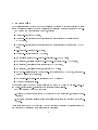
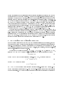
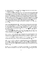
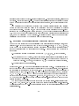
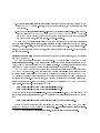
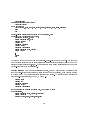
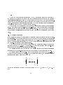
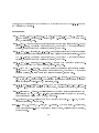
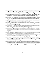
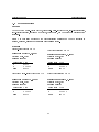
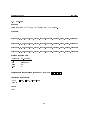
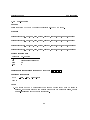
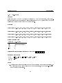
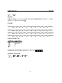
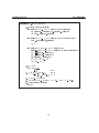
Figure 1: Selecting an iterative method.
Symmetric matrix?
Y
N
Eigenvalue
estimation?
Y
CGEV
Eigenvalue
estimation?
N
CG
CHEBYSHEV
Y
RGMRESEV
N
Transpose
matrix-vector product
available?
Y
Notes:
(1) only for mildly nonsymmetric systems
(2) use a small restarting
value if storage is at
a premium
Bi-CG
CGNR
CGNE
QMR
N
CG (1)
CGS
Bi-CGSTAB
RBi-CGSTAB
TFQMR
RGMRES (2)
RGCR (2)
CHEBYSHEV
To conclude this section, Figure 1 shows a diagram to aid in the selection of an iterative
method.
3 Internal details of PIM
3.1 Supported architectures and environments
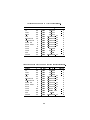
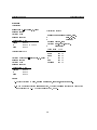
PIM has been tested on scalar, vector and parallel computers including the Cray Y-MP2E/232,
Cray Y-MP C90/16256, SGI Challenge, Intel Paragon, TMC CM-52 and networks of workstations under PVM 3.3.6, CHIMP/MPI v1.2, Argonne MPI, p4 v1.2, TCGMSG 4.02 and Intel
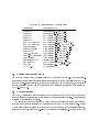
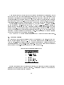
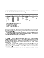
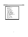
NX. Table 1 lists the architectures and environments on which PIM has been successfully tested.
2 The results obtained are based upon a beta version of the software and, consequently, is not necessarily
representative of the performance of the full version of this software.
13
Table 1: Computers where PIM has been tested
Architecture
Sun SPARC
Sun SPARC
Sun SPARC
Sun SPARC
Sun SPARC
DEC AXP 4000/610
DEC AXP 3000/800
SGI IRIS Indigo
SGI IRIS Crimson
SGI Indy II
Cray Y-MP2E/232
Cray Y-MP C90/16256
SGI Challenge
Intel Paragon XP/S
IBM 9076 SP/1
Cray T3D
TMC CM-5
Compiler and O/S
Sun Fortran 1.4 - SunOS 4.1.3
Sun Fortran 2.0.1 - SunOS 5.2
EPC Fortran 77 - SunOS 4.1.3
EPC Fortran 90 - SunOS 4.1.3
NAG Fortran 90 - SunOS 4.1.3
DEC Fortran 3.3-1 - DEC OSF/1 1.3
DEC Fortran 3.4-480 - DEC OSF/1 2.0
MIPS Fortran 4.0.5 - SGI IRIX 4.0.5F
MIPS Fortran 4.0.5 - SGI IRIX 4.0.5C
MIPS Fortran 5.0 - SGI IRIX 5.1.1
Cray Fortran 6.0 - UNICOS 7.0.5.2
Cray Fortran 7.0 - UNICOS 8.2.3
MIPS Fortran 5.2 - SGI IRIX 5.2
Portland if77 4.5 - OSF/1 1.2.6
IBM XL Fortran 6000 2.3 - AIX 3.2
Cray Fortran 8.0 - UNICOS 8.3.3
CM Fortran 77
3.2 Parallel programming model
PIM uses the Single Program, Multiple Data (SPMD) programming model. The main implication of using this model is that certain scalar values are needed in each processing element (PE).
Two of the user-supplied routines, to compute a global sum and a vector norm, must provide
for this, preferably making use of a reduction and/or broadcast routine like those present on
PVM 3.3.6 and MPI.
3.3 Data partitioning
With PIM, the iterative method routines have no knowledge of the way in which the user has
chosen to store and access either the coecient or the preconditioning matrices. We thus restrict
ourselves to partitioning the vectors.
The assumption made is that each PE knows the number of elements of each vector stored
in it and that all vector variables in a processor have the same number of elements. This is
a broad assumption that allows us to accommodate many dierent data partitioning schemes,
including contiguous, cyclic (or wrap-around) and scattered partitionings. We are able to make
14
this assumption because the vector-vector operations used { vector accumulations, assignments
and copies { are disjoint element-wise. The other operations used involving matrices and vectors
which may require knowledge of the individual indices of vectors, are the responsibility of the
user.
PIM requires that the elements of vectors must be stored locally starting from position
1; thus the user has a local numbering of the variables which can be translated to a global
numbering if required. For example, if a vector of 8 elements is partitioned in wrap-around
fashion among 2 processors, using blocks of length 1, then the rst processor stores elements
1, 3, 5 and 7 in the rst four positions of an array; the second processor then stores elements
2, 4, 6 and 8 in positions 1 to 4 on its array. We stress that for most of the commonly used
partitioning schemes data may be retrieved with very little overhead.
3.4 Increasing the parallel scalability of iterative methods
One of the main causes for the poor scalability of implementations of iterative methods
on
Pn
T
distributed-memory computers is the need to compute inner-products, = u v = i=1 ui vi ,
where u and v are vectors distributed across p processors (without loss of generality assume
that each processor holds n=p elements of each vector). This computation can be divided in
three parts
1. The local computation of partial sums of the form j = Pn=p
i=1 ui vi , on each processor,
2. The reduction of the j values, where these values travel across the processors in some
ecient way (for instance, as if traversing a binary-tree
up to its root) and are summed
P
during the process. At the end, the value of = pj=1 j is stored in a single processor,
3. The broadcast of to all processors.
During parts 2. and 3. a number of processors are idle for some time. A possible strategy to
reduce this idle time and thus increase the scalability of the implementation, is to re-arrange
the operations in the algorithm so that parts 2. and 3. accumulate a number of partial sums
corresponding to some inner-products. Some of the algorithms available in PIM, including
CG, CGEV, Bi-CG, CGNR and CGNE have been rewritten using the approach suggested by
D'Azevedo and Romine [15]. Others, like Bi-CGSTAB, RBi-CGSTAB, RGCR, RGMRES and
QMR have not been re-arranged but some or all of their inner-products can be computed with
a single global sum operation.
The computation of the last two parts depends on the actual message-passing library being
used. With MPI, parts 2. and 3. are also oered as a single operation called MPI ALLREDUCE.
Applications using the PVM 3.3.6 Fortran interface should however call PVMFREDUCE and then
PVMFBROADCAST.
15
An important point to make is that we have chosen modications to the iterative methods
that reduce the number of synchronization points while at the same time maintaining their
convergence properties and numerical qualities. This is the case of the D'Azevedo and Romine
modication; also, in the specic case of GMRES, which uses the Arnoldi process (a suitable
reworking of the modied Gram-Schmidt procedure) to compute a vector basis, the computation
of several inner-products with a single global sum does not compromise numerical stability.
For instance, in the algorithm for the restarted GMRES (see Algorithm A.9), step 5 involves
the computation of j inner-products of the form ViT Vj , i = 1; 2; : : : ; j . It is thus possible to
arrange for each processor to compute j partial sums using the BLAS routine DOT and store
these in an array. Then in a single call to a reduction routine, these arrays are communicated
among the processors and their individual elements are summed. On the completion of the
global sum the array containing the respective j inner-products is stored in a single processor
and is then broadcast to the remaining processors.
The CGS and TFQMR implementations available on PIM do not benet from this approach.
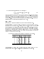
3.5 Stopping criteria
PIM oers a number of stopping criteria which may be selected by the user. In Table 2 we
list the dierent criteria used; rk = b ; Axk is the true residual of the current estimate xk ,
zk is the pseudo-residual (usually generated by linear recurrences and possibly involving the
preconditioners) and " is the user-supplied tolerance. Note that the norms are not indicated;
these depend on the user-supplied routine to compute a vector norm.
Table 2: Stopping criteria available on PIM
No.
1
2
3
4
5
6
7
Stopping criterion
jj rk jj < "
jjqrk jj < "jj b jj
rkT zk < "jj b jj
jj zk jj < "
jj zk jj < "jj b jj
jj zk jj < "jj Q1b jj
jj xk ; xk;1 jj < "
If speed of execution is of the foremost importance, the user needs to select the stopping
criterion that will impose the minimum overhead. The following notes may be of use in the
selection of an appropriate stopping criterion
16
1. If the stopping criterion selected is one of 1, 2 or 3 then the true residual is computed
(except when using TFQMR with either no preconditioning or left preconditioning).
2. The restarted GMRES method uses its own stopping criterion (see [42, page 862]) which
is equivalent to the 2-norm of the residual (or pseudo-residual if preconditioning is used).
3. If either no preconditioning or right-preconditioning is used and criterion 6 is selected,
the PIM iterative method called will ag the error and exit without solving the system
(except for the restarted GMRES routine).
4 Using PIM
4.1 Naming convention of routines
The PIM routines have names of the form
PIM method
where indicates single-precision (S), double-precision (D), complex (C) or double-precision
complex (Z) and method is one of: CG, CGEV (CG with eigenvalue estimation), CGNR, CGNE,
BICG, CGS, BICGSTAB, RBICGSTAB, RGMRES, RGMRESEV (RGMRES with eigenvalue estimation),
and RGCR, QMR, TFQMR and CHEBYSHEV.
4.2 Obtaining PIM
PIM 2.0 is available via anonymous ftp from
unix.hensa.ac.uk, le /pub/misc/netlib/pim/pim22.tar.Z
and
ftp.mat.ufrgs.br, le /pub/pim/pim22.tar.gz
There is also a PIM World-Wide-Web homepage which can be accessed at
http://www.mat.ufrgs.br/pim-e.html
which gives a brief description of the package and allows the reader to download the software
and related documentation.
The current distribution contains
The PIM routines in the directories single, double, complex and dcomplex
A set of example programs for sequential and parallel execution (using PVM and MPI)
in the directories examples/sequential, examples/pvm and examples/mpi,
This guide in PostScript format in the doc directory.
17
4.3 Installing PIM
To install PIM, unpack the distributed compressed (or gzipped), tar le:
uncompress pim22.tar.Z (or gunzip pim22.tar.gz)
tar xfp pim22.tar
cd pim
and edit the Makefile. The following variables may need to be modied
HOME Your top directory, e.g., /u1/users/fred
FC Your Fortran compiler of choice, usually f77
FFLAGS Flags for the Fortran compilation of main programs (example programs)
OFFLAGS Flags for the Fortran compilation of separate modules (PIM routines and modules of
examples)
NOTE: This must include at least the ag required for separate compilation (usually -c)
AR The archiver program, usually ar
HASRANLIB Either t (true) or f (false), indicating if it is necessary to use a random library
program (usually ranlib) to build the PIM library
BLASLIB Either the name of an archive le containing the BLAS library or -lblas if the library
libblas.a has been installed on a system-wide basis
PARLIB The compilation switches for any required parallel libraries. This variable must be left
blank if PIM is to be used in sequential mode. For example, if PVM 3 is to be used, then
PARLIB would be dened as
-L$(PVM ROOT)/lib/$(PVM ARCH) -lfpvm3 -lpvm3 -lgpvm3
Each iterative method routine is stored in a separate le with names in lower case following the naming convention of the routines, e.g., the routine PIMDCG is stored in the le
pim22/double/pimdcg.f.
Building the PIM core functions PIM needs the values of some machine-dependent
oating-point constants. The single- or double-precision values are stored in the les
pim22/common/smachcons.f and pim22/common/dmachcons.f respectively. Default values are
supplied for the IEEE-754 oating-point standard, and are stored separately in the les
pim/common/smachcons.f.ieee754 and pim/common/dmachcons.f.ieee754 { these are used
by default. However if you are using PIM on a computer which does not support the IEEE-754
standard, you may:
18
1. type make smachcons or make dmachcons; this will compile and execute a program which
uses the LAPACK routine LAMCH, to compute those constants, and the relevant les will
be generated.
2. edit either pim/common/smachcons.f.orig or pim/common/dmachcons.f.orig and replace the strings MACHEPSVAL, UNDERFLOWVAL and OVERFLOWVAL by the values of the machine epsilon, underow and overow thresholds to those of the particular
computer you are using, either in single- or double-precision.
To build PIM, type make makefiles to build the makeles in the appropriate directories
and then make single, make double, make complex or make dcomplex to build the singleprecision, double-precision, complex or double complex versions of PIM. This will generate .o
les, one for each iterative method routine, along with the library le libpim.a which contains
the support routines.
Building the examples Example programs are provided for sequential use, and for parallel
use with MPI and PVM3 .
The example programs require a timing routine. The distribution comes with the le
examples/common/timer.f which contains examples of the timing functions available on the
Cray, the IBM RS/6000 and also the UNIX etime function. By default, the latter is used; this
le must be modied to use the timing function available on the target machine.
The PVM and MPI example programs use the Fortran INCLUDE statement to include the
PVM and MPI header les. Some compilers have a switch (usually -I) which allows the user
to provide search directories in which les to be included are located (as with the IBM AIX
XL Fortran compiler); while others require the presence of those les in the same directory as
the source code resides. In the rst case, you will need to include in the FFLAGS variable the
relevant switches (see x4.3); in the latter, you will need to install the PVM and MPI header
les (fpvm3.h and mpif.h respectively) by typing
make install-pvm-include INCFILE=<name-of-fpvm3.h>
make install-mpi-include INCFILE=<name-of-mpif.h>
where you should replace <name-of-fpvm3.h> and <name-of-mpif.h> by the full lename of
the required include les; for instance, if PVM is installed on /usr/local/pvm3 then you should
type
make install-pvm-include INCFILE=/usr/local/pvm3/include/fpvm3.h
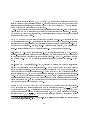
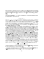
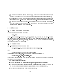
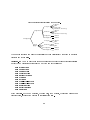
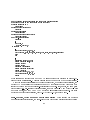
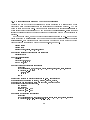
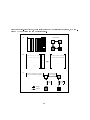
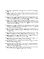
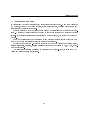
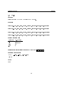
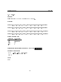
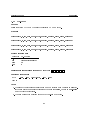
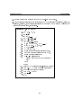
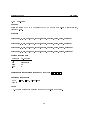
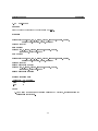
Figure 2 shows the directory tree containing the examples. To build them, type make
followed by the name of a subdirectory of examples, e.g., make sequential/single/dense.
3 The PVM examples use the \groups" library libgpvm.a which provides the reduction functions.
19
Figure 2: Directories containing the examples.
single
sequential
double
complex
dcomplex
examples
double
dense
pde
dense
pde
complex
dcomplex
dense
dense
single
pvm
mpi
dense
pde
pvp-pde
harwell-boeing
dense
pde
harwell-boeing
dense
dense
The example programs can also be built locally in those directories by changing to a specic
directory and typing make.
Cleaning-up You may wish to remove some or all of the compiled codes or other les installed
under the PIM directory; in this case you may type one of the following
make
make
make
make
make
make
make
make
make
make
make
make
singleclean
doubleclean
complexclean
dcomplexclean
sequentialclean
pvmclean
mpiclean
clean-pvm-include
clean-mpi-include
examplesclean
makefilesclean
realclean
which will clean-up the PIM routines, the examples, the Makeles, the include les and all
generated les, returning the package to its distribution form.
20
Using PIM in your application To use PIM with your application, link your program with
the .o le corresponding to the PIM iterative method routine being called and with the PIM
support library libpim.a.
4.4 Calling a PIM iterative method routine
With the exception of the Bi-CG, CGNR, CGNE and QMR methods, all the implemented
methods have the same parameter list as CG. The argument list for the double-precision implementation of the CG method is
SUBROUTINE PIMDCG(X,B,WRK,IPAR,DPAR,MATVEC,PRECONL,PRECONR,
+
PDSUM,PDNRM,PROGRESS)
and for Bi-CG (as well as for CGNR, CGNE and QMR)
SUBROUTINE PIMDBICG(X,B,WRK,IPAR,DPAR,MATVEC,TMATVEC,PRECONL,PRECONR,
PDSUM,PDNRM,PROGRESS)
+
where the parameters are as follows
Parameter Description
X
A vector of length IPAR(4)
On input, contains the initial estimate
On output, contains the last estimate computed
B
The right-hand-side vector of length IPAR(4)
WRK
A work vector used internally (see the description
of each routine for its length)
IPAR
An integer array containing input-output parameters
PAR
A oating-point array containing input-output parameters
MATVEC
Matrix-vector product external subroutine
TMATVEC
Transpose-matrix-vector product external subroutine
PRECONL
Left-preconditioning external subroutine
PRECONR
Right-preconditioning external subroutine
P SUM
Global sum (reduction) external function
P NRM
Vector norm external function
PROGRESS
Monitoring routine
Note in the example above that, contrary to the proposal in [5], PIM uses separate routines
to compute the matrix-vector and transpose-matrix-vector products. See the reference manual,
sections A.1 and A.2 for the description of the parameters above and the synopsis of the external
routine.
21
4.5 External routines
As stated earlier, the user is responsible for supplying certain routines to be used internally by
the iterative method routines. One of the characteristics of PIM is that if external routines are
not required by an iterative method routine they are not called (the only exception being the
monitoring routines). The user only needs to provide those subroutines that will actually be
called by an iterative method routine, depending on the selection of method, preconditioners
and stopping criteria; dummy parameters may be passed in place of those that are not used.
Some compilers may require the presence of all routines used in the program during the linking
phase of the compilation; in this case the user may need to provide stubs for the dummy
routines. Section A.2 gives the synopsis of each user-supplied external routine used by PIM.
The external routines have a xed parameter list to which the user must adhere (see xA.2).
Note that (from version 2.2 onwards) the coecient and the preconditioning matrices do not
appear in the parameter list of the PIM routines. Indeed we regard the matrix-vector products
and preconditioning routines as operators returning only the appropriate resulting vector; thus
the PIM routines have no knowledge of the way in which the matrices are stored.
The external routines, however, may access the matrices declared in the main program via
COMMON blocks. This strategy hides from the PIM routines details of how the matrices are
declared in the main program and thus allows the user to choose the most appropriate storage
method for her problem; previous versions of PIM were more restrictive in this sense.
Matrix-vector product Consider as an example a dense matrix partitioned by contiguous
columns among a number of processors. For illustrative purposes we assume that N is an integer
multiple of NPROCS, and that LOCLEN=N/NPROCS. The following code may then be used
PROGRAM MATV
* A IS DECLARED AS IF USING A COLUMN PARTITIONING FOR AT LEAST
* TWO PROCESSORS.
INTEGER LDA
PARAMETER (LDA=500)
INTEGER LOCLEN
PARAMETER (LOCLEN=250)
DOUBLE PRECISION A(LDA,LOCLEN)
COMMON /PIMA/A
* SET UP PROBLEM SOLVING PARAMETERS FOR USE BY USER DEFINED ROUTINES
* THE USER MAY NEED TO SET MORE VALUES OF THE IPAR ARRAY
* LEADING DIMENSION OF A
IPAR(1)=LDA
* NUMBER OF ROWS/COLUMNS OF A
IPAR(2)=N
* NUMBER OF PROCESSORS
22
IPAR(6)=NPROCS
* NUMBER OF ELEMENTS STORED LOCALLY
IPAR(4)=N/IPAR(6)
* CALL PIM ROUTINE
CALL PIMDCG(X,B,WRK,IPAR,DPAR,MATVEC,PRECONL,PRECONR,PDSUM,PDNRM,PROGRESS)
STOP
END
* MATRIX-VECTOR PRODUCT ROUTINE CALLED BY A PIM ROUTINE. THE
* ARGUMENT LIST TO THIS ROUTINE IS FIXED.
SUBROUTINE MATVEC(U,V,IPAR)
DOUBLE PRECISION U(*),V(*)
INTEGER IPAR(*)
INTEGER LDA
PARAMETER (LDA=500)
INTEGER LOCLEN
PARAMETER (LOCLEN=250)
DOUBLE PRECISION A(LDA,LOCLEN)
COMMON /PIMA/A
.
.
.
RETURN
END
The scheme above can be used for the transpose-matrix-vector product as well. We note that
many dierent storage schemes are available for storing sparse matrices; the reader may nd
useful to consult Barrett et al. [6, pp. 57] where such schemes as well as algorithms to compute
matrix-vector products are discussed.
Preconditioning For the preconditioning routines, one may use the scheme outlined above
for the matrix-vector product; in some cases this may not be necessary, when there is no need
to operate with A or the preconditioner is stored as a vector. An example is the diagonal (or
Jacobi) left-preconditioning, where Q1 = diag(A);1
PROGRAM DIAGP
INTEGER LDA
PARAMETER (LDA=500)
INTEGER LOCLEN
PARAMETER (LOCLEN=250)
* Q1 IS DECLARED AS A VECTOR OF LENGTH 250, AS IF USING AT LEAST
* TWO PROCESSORS.
DOUBLE PRECISION A(LDA,LOCLEN),Q1(LOCLEN)
COMMON /PIMQ1/Q1
EXTERNAL MATVEC,DIAGL,PDUMR,PDSUM,PDNRM
23
* SET UP PROBLEM SOLVING PARAMETERS FOR USE BY USER DEFINED ROUTINES
* THE USER MAY NEED TO SET MORE VALUES OF THE IPAR ARRAY
* LEADING DIMENSION OF A
IPAR(1)=LDA
* NUMBER OF ROWS/COLUMNS OF A
IPAR(2)=N
* NUMBER OF PROCESSORS
IPAR(6)=NPROCS
* NUMBER OF ELEMENTS STORED LOCALLY
IPAR(4)=N/IPAR(6)
* SET LEFT-PRECONDITIONING
IPAR(8)=1
.
.
.
DO 10 I=1,N
Q1(I)=1.0D0/A(I,I)
10 CONTINUE
.
.
.
CALL DINIT(IPAR(4),0.0D0,X,1)
CALL PIMDCG(X,B,WRK,IPAR,DPAR,MATVEC,DIAGL,PDUMR,PDSUM,PDNRM,PROGRESS)
STOP
END
.
.
.
SUBROUTINE DIAGL(U,V,IPAR)
DOUBLE PRECISION U(*),V(*)
INTEGER IPAR(*)
INTEGER LOCLEN
PARAMETER (LOCLEN=250)
DOUBLE PRECISION Q1(LOCLEN)
COMMON /PIMQ1/Q1
CALL DCOPY(IPAR(4),U,1,V,1)
CALL DVPROD(IPAR(4),Q1,1,V,1)
RETURN
where DVPROD is a routine based on the BLAS DAXPY routine that performs an element-byelement vector multiplication. This example also shows the use of dummy arguments (PDUMR).
Note that it is the responsibility of the user to ensure that, when using preconditioning, the
matrix Q1AQ2 must satisfy any requirements made by the iterative method being used with
respect to the symmetry and/or positive-deniteness of the matrix. For example, if A is a matrix
with arbitrary (i.e., non-constant) diagonal entries, then both diag(A);1 A and A diag(A);1 will
not be symmetric, and the CG and CGEV methods will generally fail to converge. For these
methods symmetric preconditioning, diag(A);1=2 A diag(A);1=2, should be used.
Inner-products, vector norms and global accumulation When running PIM routines
on multiprocessor architectures, the inner-product and vector norm routines require reduction
24
and broadcast operations (in some message-passing libraries these can be supplied by a single
routine). On vector processors these operations are handled directly by the hardware whereas
on distributed-memory architectures these operations involve the exchange of messages among
the processors.
When a PIM iterative routine needs to compute an inner-product, it calls DOT to compute
the partial inner-product values. The user-supplied routine P SUM is then used to generate the
global sum of those partial sums. Thepfollowing code shows the routines to compute the global
sum and the vector 2-norm jj u jj2 = uT u using the BLAS DDOT routine and the reductionplus-broadcast operation provided by MPI
SUBROUTINE PDSUM(ISIZE,X,IPAR)
INCLUDE 'mpif.h'
INTEGER ISIZE
DOUBLE PRECISION X(*)
DOUBLE PRECISION WRK(10)
INTEGER IERR,IPAR(*)
EXTERNAL DCOPY,MPI_ALLREDUCE
CALL MPI_ALLREDUCE(X,WRK,ISIZE,MPI_DOUBLE_PRECISION,MPI_SUM,
+
MPI_COMM_WORLD,IERR)
CALL DCOPY(ISIZE,WRK,1,X,1)
RETURN
END
DOUBLE PRECISION FUNCTION PDNRM(LOCLEN,U,IPAR)
INCLUDE 'mpif.h'
INTEGER LOCLEN
DOUBLE PRECISION U(*)
DOUBLE PRECISION PSUM
INTEGER IERR,IPAR(*)
DOUBLE PRECISION DDOT
EXTERNAL DDOT
INTRINSIC SQRT
DOUBLE PRECISION WRK(1)
EXTERNAL MPI_ALLREDUCE
PSUM = DDOT(LOCLEN,U,1,U,1)
CALL MPI_ALLREDUCE(PSUM,WRK,1,MPI_DOUBLE_PRECISION,MPI_SUM,
+
MPI_COMM_WORLD,IERR)
PDNRM = SQRT(WRK(1))
RETURN
END
It should be noted that P SUM is actually a wrapper to the global sum routines available on
25
a particular machine. Also, when executing PIM on a sequential computer, these routines are
empty i.e., the contents of the array X must not be altered in any way since its elements already
are the inner-product values.
The parameter list for these routines was decided upon after inspecting the format of the
global operations available from existing message-passing libraries.
Monitoring the iterations In some cases, most particularly when selecting the iterative
method to be used for solving a specic problem, it is important to be able to obtain feedback
from the PIM routines as to how an iterative method is progressing.
To this end, we have included in the parameter list of each iterative method routine an
external subroutine (called PROGRESS) which receives from that routine the number of vector elements stored locally (LOCLEN), the iteration number (ITNO), the norm of the residual (NORMRES)
(according to the norm being used), the current iteration vector (X), the residual vector (RES)
and the true residual vector rk = b ; Axk , (TRUERES). This last vector contains meaningful
values only if IPAR(9) is 1, 2 or 3.
The parameter list of the monitoring routine is xed, as shown in xA.2. The example below
shows a possible use of the monitoring routine, for the DOUBLE PRECISION data type.
SUBROUTINE PROGRESS(LOCLEN,ITNO,NORMRES,X,RES,TRUERES)
INTEGER LOCLEN,ITNO
DOUBLE PRECISION NORMRES
DOUBLE PRECISION X(*),RES(*),TRUERES(*)
EXTERNAL PRINTV
WRITE (6,FMT=9000) ITNO,NORMRES
WRITE (6,FMT=9010) 'X:'
CALL PRINTV(LOCLEN,X)
WRITE (6,FMT=9010) 'RESIDUAL:'
CALL PRINTV(LOCLEN,RES)
WRITE (6,FMT=9010) 'TRUE RESIDUAL:'
CALL PRINTV(LOCLEN,TRUERES)
RETURN
9000 FORMAT (/,I5,1X,D16.10)
9010 FORMAT (/,A)
END
SUBROUTINE PRINTV(N,U)
INTEGER N
DOUBLE PRECISION U(*)
INTEGER I
DO 10 I = 1,N
WRITE (6,FMT=9000) U(I)
10 CONTINUE
RETURN
9000 FORMAT (4(D14.8,1X))
26
END
As with the other external routines used by PIM, this routine needs to be supplied by
the user; we have included the source code for the routine as shown above in the directory
/pim/examples/common and this may be used as is or can be modied by the user as required.
Please note that for large system sizes the routine above will produce very large amounts of
output. We stress that this routine is always called by the PIM iterative method routines; if no
monitoring is needed a dummy routine must be provide.
Note that some of the iterative methods contain an inner loop within the main iteration
loop. This means that, for PIM RGCR and PIM TFQMR, the value of ITNO passed to PROGRESS
will be repeated as many times as the inner loop is executed. We did not modify the iteration
number passed to PROGRESS so as to reect the true behaviour of the iterative method being
used.
4.6 Example programs
In the distributed software the user will nd a collection of example programs under the directory examples. The example programs show how to use PIM with three dierent matrix storage
formats including dense matrices, those derived from the ve-point nite-dierence discretisation of a partial dierential equation (PDE) and the standard sparse representation found in
the Harwell-Boeing sparse matrix collection [18].
Most of the examples are provided for sequential and parallel execution, the latter with
separate codes for PVM 3.3.6 and MPI libraries. The examples involving the Harwell-Boeing
sparse format are provided for sequential execution only.
The parallel programs for the dense and PDE storage formats have dierent partitioning
strategies and the matrix-vector products have been designed to take advantage of these.
The systems solved have been set-up such that the solution is the vector x = (1; 1; : : : ; 1)T ,
in order to help in checking the results. For the dense storage format, the real system has the
tridiagonal coecient matrix of order n = 500
2
6
6
6
A = 66
6
4
4 1
1 4 1
... ... ...
1 4 1
1 4
3
7
7
7
7
7
7
5
and the complex system of order n = 100 has the form A = I + S , where S = S H , = 4 ; 4i
and
27
S
2
6
6
6
= 66
6
4
1+i
1;i 0 1+i
... ...
1;i
3
7
7
7
7
7
7
5
0
...
0
(5)
1+i
1;i 0
The problem using the Harwell-Boeing format is NOS4 from the LANPRO collection of problems
in structural engineering [18, pp. 54-55]. Problem NOS4 has order n = 100 and is derived from a
nite-element approximation of a beam structure. For the PDE storage format the system being
solved is derived from the ve-point nite-dierence discretisation of the convection-diusion
equation
!
2u
2u
@
@
@u
; @x2 + @y2 + cos() @u
(6)
@x + sin() @y = 0
on the unit square, with = 0:1, = ;=6 and u = x2 + y2 on R. The rst order terms were
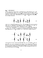
discretised using forward dierences (this problem was taken from [44]).
A dierent set of systems is used for the HYBRID examples with dense storage format. The
real system has a nonsymmetric tridiagonal coecient matrix of order n = 500
2
6
6
6
A = 66
6
4
2 ;1
2 2 ;1
... ... ...
2 2 ;1
2 2
and the complex system of order n = 100 has A dened as
2
6
6
6
A = 66
6
4
2 ;1 + i
2 + i 2 ;1 + i
...
...
2+i
3
7
7
7
7
7
7
5
3
7
7
7
7
7
7
5
...
2 ;1 + i
2+i 2
The examples include the solution of systems using dierent preconditioners. In the dense
and Harwell-Boeing formats the examples include diagonal and polynomial preconditioners; the
ve-point PDE format includes a variant of the incomplete LU factorisation and polynomial
preconditioners. The polynomial preconditioners provided are the Neumann and the weighted
and unweighted least-squares polynomials found in [36].
28
4.6.1 Eigenvalues estimation and Chebyshev acceleration
Consider the use of Chebyshev acceleration to obtain a solution to a linear system whose
coecient matrix has real entries only; the eigenvalues of the iteration matrix I ; Q1 A are
known to lie in the complex plane. We can use a few iterations of the routine PIMDRGMRESEV to
obtain estimates of the eigenvalues of Q1A and then switch to PIMDCHEBYSHEV. Before the latter
is called a transformation on the extreme values on the real axis must be made as described in
Section 2.
In the example below, we use the Jacobi preconditioner as shown in x4.5. Note that the
vector X returned by PIMDRGMRESEV may be used as an improved initial vector for the routine
PIMDCHEBYSHEV. Both routines are combined in a loop to produce a hybrid method; the code
below is based on the algorithm given by Elman et al. [21, page 847].
PROGRAM HYBRID
INTEGER MAXIT
EXTERNAL MATVEC,PRECON,PDUMR,PDSUM,PDNRM2
* SET MAXIMUM NUMBER OF ITERATIONS FOR THE HYBRID LOOP
MAXIT=INT(N/2)+1
* SET LEFT-PRECONDITIONING
IPAR(8)=1
CALL DINIT(N,0.0D0,X,1)
DO 10 I = 1,MAXIT
* SET SMALL NUMBER OF ITERATIONS FOR RGMRESEV
IPAR(10)=3
CALL PIMDRGMRESV(X,B,WRK,IPAR,DPAR,MATVEC,PRECONR,PDUMR,PDSUM,PDNRM,PROGRESS)
IF (IPAR(12).NE.-1) THEN
IPAR(11) = I
GO TO 20
END IF
*
*
*
*
MODIFY REAL INTERVAL TO REFLECT EIGENVALUES OF I-Q1A. BOX CONTAINING
THE EIGENVALUES IS RETURNED IN DPAR(3), DPAR(4), DPAR(5), DPAR(6),
THE FIRST TWO ARE THE INTERVAL ALONG THE REAL AXIS, THE LAST TWO ARE
THE INTERVAL ALONG THE IMAGINARY AXIS.
MU1 = DPAR(3)
MUN = DPAR(4)
DPAR(3) = 1.0D0 - MUN
DPAR(4) = 1.0D0 - MU1
* SET NUMBER OF ITERATIONS FOR CHEBYSHEV
IPAR(10)=5
CALL PIMDCHEBYSHEV(X,B,DWRK,IPAR,DPAR,MATVEC,PRECON,PDUMR,PDSUM,PDNRM2,PROGRESS)
IF ((IPAR(12).EQ.0) .OR. (IPAR(12).EQ.-6) .OR.
29
+
(IPAR(12).EQ.-7)) THEN
IPAR(11) = I
GO TO 20
END IF
10 CONTINUE
20 CONTINUE
.
.
.
4.6.2 Dense storage
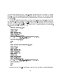
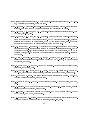
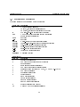
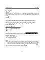
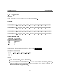
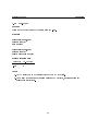
For the dense case, the coecient matrix is partitioned by columns among the p processors,
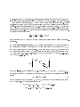
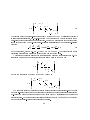
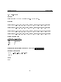
which are considered to be logically connected on a grid (see Figure 3-A). Each processor stores
at most d n=p e columns of A. For the example shown in Figure 3-B, the portion of the matrixvector product to be stored in processor 0 is computed according to the diagram shown in
Figure 3-C. Basically, each processor computes a vector with the same number of elements as
that of the target processor (0 in the example) which holds the partial sums for each element.
This vector is then sent across the network to be summed in a recursive-doubling fashion until
the accumulated vectors, carrying the contributions of the remaining processors, arrive at the
target processor. These accumulated vectors are then summed together with the partial sum
vector computed locally in the target processor, yielding the elements of the vector resulting
from the matrix-vector product. This process is repeated for all processors. This algorithm is
described in [13].
To compute the dense transpose-matrix-vector product, AT u, each processor broadcasts to
the other processors a copy of its own part of u. The resulting part of the v vector is then
computed by each processor.
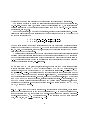
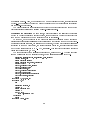
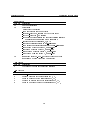
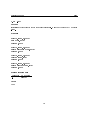
4.6.3 PDE storage
For the PDE storage format, a square region is subdivided into l + 1 rows and columns giving a
grid containing l2 internal points, each point being numbered as i +(j ; 1)l, i; j = 1; 2; : : : ; l (see
Figure 4). At each point we assign 5 dierent values corresponding to the center, north, south,
east and west points on the stencil (i;j , i;j , i;j , i;j , "i;j respectively) which are derived from
the PDE and the boundary conditions of the problem. Each grid point represents a variable;
the whole being obtained by solving a linear system of order n = l2 .
A matrix-vector product v = Au is obtained by computing
vi;j = i;j ui;j + i;j ui+1;j + i;j ui;1;j + i;j ui;j +1 + "i;j ui;j ;1
(7)
where some of the , , , and " may be zero according to the position of the point relative
to the grid. Note that only the neighbouring points in the vertical and horizontal directions are
needed to compute vi;j .
30
Figure 3: Matrix-vector product, dense storage format: A) Partitioning in columns , B) Example and C) Computation and communication steps.
Processors
A)
B)
G H
a
Aa+Bb+Cc+Dd+Ee+Ff+Gg+Hh
M N O P
b
Ia+Jb+Kc+Ld+Me+Nf+Og+Ph
A B
C D E
I
K L
J
F
c
.
=
d
.
e
f
.
g
h
C)
Aa+Bb+Cc+Dd+Ee+Ff+Gg+Hh
Ia+Jb+Kc+Ld+Me+Nf+Og+Ph
.
.
.
Cc+Dd+Gg+Hh
Kc+Ld+Og+Ph
Ee+Ff
Me+Nf
Step 1
Step 2
31
Gg+Hh
Og+Ph
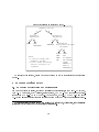
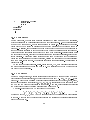
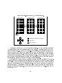
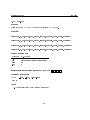
Figure 4: Matrix-vector product, PDE storage format.
Processor 0
Processor 1
Processor 2
6
5
4
3
2
8
1
7
i
j
β
ε
α
δ
γ
Boundary grid points (exchanged)
Grid points
Data exchange
Five−point stencil
A parallel computation of (7) may be organised as follows. The grid points are partitioned
by vertical panels among the processors as shown in Figure 4. A processor holds at most d l=p e
columns of l grid points. To compute the matrix-vector product, each processor exchanges with
its neighbours the grid points in the \interfaces" between the processors (the points marked
with white squares in Figure 4). Equation (7) is then applied independently by each processor
at its local grid points, except at the local interfacing points. After the interfacing grid points
from the neighbouring processors have arrived at a processor, Equation (7) is applied using the
local interfacing points and those from the neighbouring processors.
This parallel computation oers the possibility of overlapping communication with the computation. If the number of local grid points is large enough, one may expect that while Equation
(7) is being applied to those points, the interfacing grid points of the neighbouring processors
will have been transferred and be available for use. This method attempts to minimize the
overheads incurred by transferring the data (note that we only make gains if the asynchronous
transfer of messages is available). The example below is taken from the matrix-vector product
routine using MPI
32
SUBROUTINE PDMVPDE(NPROCS,MYID,LDC,L,MYL,COEFS,U,V,UEAST,UWEST)
INCLUDE 'mpif.h'
* Declarations...
* Send border U values to (myid+1)-th processor
MSGTYPE = 1000
TO = MYID + 1
CALL MPI_ISEND(U(EI0),L,MPI_DOUBLE_PRECISION,TO,MSGTYPE,
+
MPI_COMM_WORLD,SID0,IERR)
* Post to receive border U values from (myid+1)-th processor
MSGTYPE = 1001
CALL MPI_IRECV(UEAST,L,MPI_DOUBLE_PRECISION,MPI_ANY_SOURCE,
+
MSGTYPE,MPI_COMM_WORLD,RID0,IERR)
* Send border U values to (myid-1)-th processor
MSGTYPE = 1001
TO = MYID - 1
CALL MPI_ISEND(U(WI0),L,MPI_DOUBLE_PRECISION,TO,MSGTYPE,
+
MPI_COMM_WORLD,SID1,IERR)
* Post to receive border U values from (myid-1)-th processor
MSGTYPE = 1000
CALL MPI_IRECV(UWEST,L,MPI_DOUBLE_PRECISION,MPI_ANY_SOURCE,
+
MSGTYPE,MPI_COMM_WORLD,RID1,IERR)
* Compute with local grid points...
* Need "eastern" data,wait for completion of receive
CALL MPI_WAIT(RID0,ISTAT,IERR)
* Compute with local interfacing grid points in the "east"...
* Need "west" data,wait for completion of receive
CALL MPI_WAIT(RID1,ISTAT,IERR)
* Compute with local interfacing grid points in the "west"...
* Release message IDs
CALL MPI_WAIT(SID0,ISTAT,IERR)
CALL MPI_WAIT(SID1,ISTAT,IERR)
RETURN
END
The computation of the transpose-matrix-vector product for the PDE case is performed in a
similar fashion. Before the computation starts, each processor exchanges with its left and right
33
neighbouring processors the east and west coecients corresponding to the interfacing grid
points4. The computation performed is then similar to the matrix-vector product described
above except that for each interfacing grid point we apply
vi;j = i;j ui;j + i+1;j ui+1;j + i;1;j ui;1;j + "i;j +1ui;j +1 + i;j ;1ui;j ;1
(8)
Comparing (8) to (7) we see that the coecients are swapped in the north-south and east-west
directions. Note that due to the partitioning imposed we do not need to exchange the north
and south coecients.
A matrix-vector product for parallel vector architectures For parallel vector architec-
tures like the Cray Y-MP2E, the routines outlined above are not ecient, because of the small
vector lengths involved. A routine requiring the use of long vectors may be obtained by writing
the matrix-vector product for the 5-point stencil as a sequence of AXPYs. The use of AXPYs
also provides a better performance because these operations are usually very ecient on such
machines.
Consider the storage scheme described above i.e., ve coecients (, , , and ") are stored
per grid point, and numbered sequentially as i + (j ; 1)l, i; j = 1; 2; : : : ; l. The coecients can
then be stored in ve separate arrays of size n = l2. The matrix-vector product v = Au can
then be obtained by the following sequence of operations
vk = k uk ; k = 1; 2; : : : ; n
(9)
vk = vk + k uk+1; k = 1; 2; : : : ; n ; 1
(10)
vk = vk + k uk;1; k = 2; 3; : : : ; n
(11)
vk = vk + k uk+l ; k = 1; 2; : : : ; n ; l
(12)
vk = vk + "k uk;l ; k = l + 1; l + 2; : : : ; n
(13)
and the transpose matrix-vector product v = AT u is obtained similarly,
vk = k uk ; k = 1; 2; : : : ; n
(14)
vk+1 = vk+1 + k uk ; k = 1; 2; : : : ; n ; 1
(15)
vk;1 = vk;1 + k uk ; k = 2; 3; : : : ; n
(16)
vk+l = vk+l + k uk ; k = 1; 2; : : : ; n ; l
(17)
vk;l = vk;l + "k uk ; k = l + 1; l + 2; : : : ; n
(18)
Experiments on the Cray Y-MP2E/232 showed that this approach gave a three-fold improvement in the performance, from 40MFLOPS to 140MFLOPS. A separate set of the PDE examples
containing these matrix-vector product routines are provided under the
pim22/examples/sequential/pvp-pde directory.
4 This may only need to be done once if the coecient matrix is unchanged during the solution of the system.
34
4.6.4 Preconditioners
The examples involving an incomplete LU factorisation as the preconditioner for the PDE case
are a modication of the usual ILU(0) method. This modication was made to allow the computation of the preconditioning step without requiring any communication to be performed. To
achieve this we note that the matrices arising from the ve-point nite-dierence discretisation
have the following structure
2
6
6
A = 666
4
3
2
3
B E
7
6
7
.
.
7
6
7
.
F B .
7 ; B = 6 ..
7
(19)
7
6
7
. . . . . . E 75
.
.
6
.
.
. . 75
4
F B
where E and F are diagonal matrices and , and are the central, north and south coecients
derived from the discretisation (the subscripts are dropped for clarity). Each matrix B is
approximating the unknowns in a single vertical line on the grid on Figure 4.
To compute a preconditioner Q = LU , we modify the ILU(0) algorithm in the sense that
the blocks E and F are discarded (because only the diagonal blocks are considered we refer to
this factorisation as IDLU(0)). The resulting L and U factors have the following structure
2
6
6
= 66
4
X
3
7
7
7;
7
5
2
6
6
= 66
4
3
1
7
X
1
7
L
X
...
. . . . . . 775 ;
X
1
2
3
2
3
Y
6
6
7
. . . 77
6
Y
6
7
6
7
6
7
U =6
7
...
7; Y = 6
.
6
.
4
5
. 75
4
Y
(20)
where , and are the modied coecients arising from the ILU(0) algorithm. >From the
structure of L and U it may be clearly seen that applying the preconditioning step reduces to the
solution of small (order l), independent, triangular systems. Each of these systems correspond
to a vertical line in the grid; since it was partitioned in vertical panels, these systems can be
solved independently in each processor.
35
The polynomial preconditioners used can be expressed by
m
X
i=0
!
i
m;i I ; (diag(A));1 A (diag(A));1
(21)
which can be easily computed as a sequence of vector updates and matrix-vector products using
Horner's algorithm. Note that the m;i coecients dene the kind of polynomial preconditioner
being used. The Neumann preconditioner is obtained when m;i = 1; 8i ; the weighted and
unweighted least-squares polynomial preconditioners are those reported in [36]. The maximum
available degree of the polynomial for these latter two is m = 13.
4.6.5 Results
In this section we provide some results for the example programs discussed above.
Stopping criteria As pointed out earlier, the selection of the stopping criterion has a sub-
stantial eect on the execution time. Evidently, there is a trade-o between the time spent
on each iteration and the total number of iterations required for convergence. In Table 3 we
show, for each of the stopping criteria provided, the execution time per iteration when PIMDCG
is applied to the tridiagonal system (described in x4.6) of order n = 500 with diagonal leftpreconditioning. The increase in execution time of each stopping criterion with respect to
criterion 4 (the \cheapest" one) is shown.
Table 3: Eect of dierent stopping criteria on an iterative method routine.
Stopping
criterion
1
2
3
4
5
6
7
k
19
15
14
18
14
15
19
Time(s)/
jj rk jj2
iteration Increase
;
11
3:56 10
0:3331
2:66
6:91 10;9 0:3531
2:79
1:29 10;8 0:3286
2:62
;
11
3:32 10
0:1254
;;
6:45 10;9 0:1967
1:57
1:73 10;9 0:2904
2:32
3:70 10;11 0:4148
3:31
General results We present below the results obtained from solving a system of n = 64
equations derived from the 5-point nite-dierences discretisation of Equation (6).
36
We used both the IDLU(0) and the Neumann polynomial preconditioner of degree 1 as leftpreconditioners to solve this problem. The stopping criterion used was number 5 with " = 10;10
and the 2-norm; using this criterion a solution will be accepted if jj zk jj2 < 3:802 10;14 , except
for PIMDRGMRES which stops its iterations when the norm of the residual is less than ". The
maximum number of iterations allowed was 32 and the initial value of the solution vector was
(0; 0; : : : ; 0)T . For the restarted GMRES and GCR the restarting value used was 10. The results
are reported for the double-precision versions of the routines.
Tables 4 and 5 show the results obtained with the PIM routines for the IDLU(0) and
Neumann preconditioners on a single workstation. A status value of 0 on exit from a PIM
routine indicates that the convergence conditions have been satised; a non-zero status value
indicates that a problem has been encountered. In particular a status value of ;1 is returned
when the maximum number of iterations specied by the user has been exceeded. This example
is characteristic of the problems facing the user of iterative method i.e., not all methods converge
to the solution and some preconditioner may cause an iterative method to diverge (or converge
slowly). We stress that the methods that have failed to converge in this example do converge
for other systems.
Scalability In Table 6 we present the execution times obtained by solving the test problem
above, but with n = 16384 equations, with the PIMDRGMRES routine (using 10 basis vectors)
and the Neumann polynomial preconditioner (of rst degreee) on the IBM SP/1, Intel Paragon
XP/S, Kendall Square Research KSR1, SGI Challenge, Cray Y-MP2E and Cray C9016E. The
PIMDRGMRES routine converged to a tolerance of 10;13 in 70 iterations. The results for the Cray
machines were obtained with the modied matrix-vector product routines described in x4.6.3.
The results for the KSR1 are obtained using the KSRBLAS routines. The programs running
on the SGI Challenge are from the set of examples available with the PIM distributed software
using the PVM message-passing library. The results for the IBM SP/1 are obtained using
the IBM PVMe 2.0 version of PVM, which enables the use of the IBM SP/1 High Performance
Switch. Note that for the IBM SP/1, SGI Challenge and Intel Paragon XP/S superlinear eects
occur; we believe this is due to the specic memory organization of those machines (hierarchic
memories and/or the presence of a cache memory).
5 Summary
We have described in this report PIM, the Parallel Iterative Methods package, a collection of
Fortran 77 routines for the parallel solution of linear systems using iterative methods.
The package was designed to be used in a variety of parallel environments without imposing
any restriction on the way the coecient matrices and the preconditioning steps are handled.
The user may thus explore characteristics of the problem and of the particular parallel architec37
Table 4: Example with IDLU(0) preconditioner.
Method
CG
CGEV
Bi-CG
CGS
Bi-CGSTAB
RBi-CGSTAB
RGMRES
RGMRESEV
RGCR
CGNR
CGNE
QMR
TFQMR
k Time(s)
jj r(k ) jj2
Status
32 0:0900
59:8747
;1
32 0:1500
59:8747
;1
32 0:1000
10:8444
;1
;
11
11 0:0500 1:8723 10
0
12 0:0400 1:1099 10;11
0
;
12
7 0:0300 3:7795 10
0
3 0:0600 2:8045 10;12
0
3 0:4500 2:8045 10;12
0
;
12
3 0:0800 2:8048 10
0
32 0:0800
81:5539
;1
32 0:0900
37:0570
;1
32 0:1200
4:0091
;1
11 0:0500 5:3482 10;11
0
Table 5: Example with Neumann polynomial preconditioner.
Method
CG
CGEV
Bi-CG
CGS
Bi-CGSTAB
RBi-CGSTAB
RGMRES
RGMRESEV
RGCR
CGNR
CGNE
QMR
TFQMR
k Time(s)
jj r(k ) jj2
Status
32 0:1000
41:9996
;1
32 0:1300
41:9996
;1
32 0:1000
13:8688
;1
14 0:0500 7:4345 10;11
0
;
12
14 0:0500 5:3863 10
0
8 0:0500 8:4331 10;14
0
3 0:0600 4:0454 10;11
0
;
11
3 0:3900 4:0454 10
0
3 0:0900 4:0455 10;11
0
;
1
32 0:0800 7:4844 10
;1
32 0:1000 3:6205 102
;1
32 0:1600
2:3351
;1
;
11
14 0:1100 7:6035 10
0
38
Table 6: Execution time (in seconds) for test problem (n = 16384) solved by PIMDRGMRES with
the Neumann polynomial preconditioner (of rst degreee).
p
1
2
4
8
16
32
?
IBM
Intel
Intel
SGI
?
SP/1 Paragon XP/S iPSC/860 Challengey
150:42
265:83
99:60
39:60
131:64
80:90
20:43
60:54
46:95
26:73
7:10
29:82
31:62
16:35
35:38
11:20
Cray
Cray
Cray
KSR1z T3D Y-MP2E C9016
453:20
297:40
166:80
11:64
4:99
4:04
W.H. Purvis, Daresbury Laboratory, U.K.
y S. Thomas, CERCA/Montreal
z A. Pindor, U. of Toronto [39]
P.T.M. Bulh~oes, Cray Research Inc.
ture being used. Indeed, the performance of a PIM routine is dependent on the user-supplied
routines for the matrix-vector products, inner-products and vector norms and the computation
of the preconditioning steps.
PIM is an ongoing project and we intend to improve it and include other iterative methods.
We encourage readers to send their comments and suggestions; the authors may be contacted
via e-mail at either [email protected] or [email protected] .
Acknowledgements
We would like to thank the National Supercomputing Centre (CESUP), Brazil, the National
Laboratory for Scientic Computing (LNCC/CNPq), Brazil, the Parallel Laboratory, University
in Bergen, Norway, the Army High Performance Computing Research Center, Minnesota, USA
and Digital Equipment Corporation (via the Internet Alpha Program), who kindly made their
facilities available for our tests.
We also thank our collaborators, Matthias G. Imhof (MIT), Paulo Tiberio M. Bulh~oes (Cray
Research), Steve Thomas (CERCA/Montreal), Andrzej Pindor (University of Toronto), William
H. Purvis (Daresbury Laboratory, U.K.) and Ramiro B. Willmersdorf (LNCC, Brazil) for their
help on testing PIM.
This work was supported in part by the Army High Performance Computing Research
39
Center, under the auspices of Army Research Oce contract number DAAL03-89-C-0038 with
the University of Minnesota.
References
[1] E. Anderson, Z. Bai, C. Bischof, J. Demmel, J. Dongarra, J. Du Croz, A. Greenbaum,
S. Hammarling, A. McKenney, S. Ostrouchov, and D. Sorensen. LAPACK Users' Guide.
SIAM, Philadelphia, 1992.
[2] S.F. Ashby. Minimax polynomial preconditioning for Hermitian linear systems. Report
UCRL-JC-103201, Numerical Mathematics Group, Computing & Mathematics Research
Division, Lawrence Livermore National Laboratory, March 1990.
[3] S.F. Ashby, T.A. Manteuel, and J.S. Otto. A comparison of adaptive Chebyshev and least
squares polynomial preconditioning for Hermitian positive denite linear systems. Report
UCRL-JC-106726, Numerical Mathematics Group, Computing & Mathematics Research
Division, Lawrence Livermore National Laboratory, March 1991.
[4] S.F. Ashby, T.A. Manteuel, and P.E. Saylor. A taxonomy for Conjugate Gradient methods. SIAM Journal of Numerical Analysis, 27:1542{1568, 1990.
[5] S.F. Ashby and M.K. Seager. A proposed standard for iterative linear solvers (version
1.0). Report UCRL-102860, Numerical Mathematics Group, Computing & Mathematics
Research Division, Lawrence Livermore National Laboratory, January 1990.
[6] R. Barrett, M. Berry, T. Chan, J. Demmel, J. Donald, J. Dongarra, V. Eijkhout, R. Pozo,
C. Romine, and H. van der Vorst. Templates for the solution of linear systems: building
blocks for iterative methods. SIAM, Philadelphia, 1993.
[7] R.A.A. Bruce, J.G. Mills, and G.A. Smith. CHIMP/MPI user guide. EPCC-KTP-CHIMPV2-USER 1.2, Edinburgh Parallel Computer Centre, University of Edinburgh, June 1994.
[8] H.M. Bucker and M. Sauren. A parallel version of the unsymmetric Lanczos algorithm and
its application to QMR. KFA-ZAM-IB-9605, Zentralinstitut fur Angewandte Mathematik,
Forschungszentrum Julich Gmbh (KFA), March 1996.
[9] R. Butler and E. Lusk. User's guide to the p4 programming system. ANL-92/17, Argonne
National Laboratory, October 1992.
[10] F.-C. Cheng, P. Vaughan, D. Reese, and A. Skjellum. The Unify system. User's guide,
document for version 0.9.2, NSF Engineering Research Center, Mississippi State University,
September 1994.
40
[11] E.J. Craig. The N-step iteration procedures. Journal of Mathematical Physics, 34:64{73,
1955.
[12] R.D. da Cunha. A Study on Iterative Methods for the Solution of Systems of Linear
Equations on Transputer Networks. PhD thesis, Computing Laboratory, University of
Kent at Canterbury, July 1992.
[13] R.D. da Cunha and T.R. Hopkins. Parallel preconditioned Conjugate-Gradients methods
on transputer networks. Transputer Communications, 1(2):111{125, 1993. Also as TR-5-93,
Computing Laboratory, University of Kent at Canterbury, U.K.
[14] R.D. da Cunha and T.R. Hopkins. A parallel implementation of the restarted GMRES
iterative method for nonsymmetric systems of linear equations. Advances in Computational Mathematics, 2(3):261{277, April 1994. Also as TR-7-93, Computing Laboratory,
University of Kent at Canterbury.
[15] E.F. D'Azevedo and C.H. Romine. Reducing communication costs in the Conjugate Gradient algorithm on distributed memory multiprocessors. Research Report ORNL/TM-12192,
Oak Ridge National Laboratory, 1992.
[16] J.J. Dongarra, J. Du Croz, S. Hammarling, and R.J. Hanson. An extended set of FORTRAN Basic Linear Algebra Subprograms. ACM Transactions on Mathematical Software,
14(1):1{17, 1988.
[17] J.J. Dongarra, R.A. van de Geijn, and R.C. Whaley. A users' guide to the BLACS v0.1.
Technical report, Computer Science Department, University of Tennessee, 1993.
[18] I.S. Du, R.G. Grimes, and J.G. Lewis. Users' guide for the Harwell-Boeing sparse matrix
collection. Report TR/PA/92/86, CERFACS, October 1992.
[19] I.S. Du, M. Marrone, and G. Radicati. A proposal for user level sparse BLAS { SPARKER
working note #1. Report TR/PA/92/85, CERFACS, October 1992.
[20] S.C. Eisenstat. A note on the generalized Conjugate Gradient method. SIAM Journal of
Numerical Analysis, 20:358{361, 1983.
[21] H.C. Elman, Y. Saad, and P. Saylor. A hybrid Chebyshev Krylov subspace algorithm
for solving nonsymmetric systems of linear equations. SIAM Journal of Scientic and
Statistical Computing, 7:840{855, 1986.
[22] R. Fletcher. Conjugate Gradient Methods for Indenite Systems, volume 506 of Lecture
Notes in Mathematics, pages 73{89. Spring-Verlag, Heidelberg, 1976.
41
[23] Message Passing Interface Forum. MPI: A message-passing interface standard. TR CS-93214, University of Tennessee, November 1993.
[24] R.W. Freund. A transpose-free quasi-minimal residual algorithm for non-Hermitian linear
systems. Submitted to SIAM Journal of Scientic and Statistical Computing.
[25] R.W. Freund, G.H. Golub, and N.M. Nachtigal. Iterative solution of linear systems. Acta
Numerica, 1:57{100, 1991.
[26] R.W. Freund, G.H. Golub, and N.M. Nachtigal. Recent advances in Lanczos-based iterative methods for nonsymmetric linear systems. RIACS Technical Report 92.02, Research
Institute for Advanced Computer Science, NASA Ames Research Center, 1992. To appear
on Algorithmic trends for Computational Fluid Dynamics in the 90's.
[27] R.W. Freund and M. Hochbruck. A Biconjugate Gradient-type algorithm for the iterative solution of non-Hermitian linear systems on massively parallel architectures. RIACS
Technical Report 92.08, Research Institute for Advanced Computer Science, NASA Ames
Research Center, 1992. To appear on Computational and Applied Mathematics I-Algorithms
and Theory.
[28] A. Geist, A. Beguelin, J. Dongarra, W. Jiang, R. Manchek, and V.S. Sunderam. PVM 3
user's guide and reference manual. Research Report ORNL/TM-12187, Oak Ridge National
Laboratory, May 1993.
[29] G.H. Golub and C.F. Van Loan. Matrix Computations. Johns Hopkins University Press,
Baltimore, 2nd edition, 1989.
[30] R.G. Grimes, D.R. Kincaid, and D.M. Young. ITPACK 2.0 user's guide. Report No.
CNA-150, Center for Numerical Analysis, University of Texas at Austin, August 1979.
[31] W. Gropp and B. Smith. Simplied linear equation solvers users manual. ANL-93/8,
Argonne National Laboratory, February 1993.
[32] L.A. Hageman and D.M. Young. Applied Iterative Methods. Academic Press, New York,
1981.
[33] R.J. Harrison. TCGMSG Send/receive subroutines { version 4.02. User's manual, Battelle
Pacic Northwest Laboratory, January 1993.
[34] M.A. Heroux. A proposal for a sparse BLAS toolkit { SPARKER working note #2. Report
TR/PA/92/90, CERFACS, October 1992.
[35] M.R. Hestenes and E.L. Stiefel. Method of Conjugate Gradients for solving linear systems.
Journal of Research National Bureau of Standards, 49:435{498, 1952.
42
[36] W.H. Holter, I.M. Navon, and T.C. Oppe. Parallelizable preconditioned Conjugate Gradient methods for the Cray Y-MP and the TMC CM-2. Technical report, Supercomputer
Computations Research Institute, Florida State University, December 1991.
[37] N.M. Nachtigal, S.C. Reddy, and L.N. Trefethen. How fast are nonsymmetric matrix
iterations. SIAM Journal on Matrix Analysis and Applications, 13(3):778{795, 1992.
[38] T.C. Oppe, W.D. Joubert, and D.R. Kincaid. NSPCG user's guide { version 1.0. Report
No. CNA-216, Center for Numerical Analysis, University of Texas at Austin, April 1988.
[39] A. Pindor. Experiences with implementing PIM (Parallel Iterative Methods) package on
KSR1. In Supercomputing Symposium '94, Toronto, June 1994.
[40] Y. Saad. Krylov subspace methods for solving large unsymmetric systems. Mathematics
of Computation, 37:105{126, 1981.
[41] Y. Saad and M.H. Schultz. Conjugate Gradient-like algorithms for solving nonsymmetric
linear systems. Mathematics of Computation, 44(170):417{424, 1985.
[42] Y. Saad and M.H. Schultz. GMRES: a generalized minimal residual algorithm for solving
nonsymmetric linear systems. SIAM Journal of Scientic and Statistical Computing, 7:856{
869, 1986.
[43] G.L.G. Sleijpen and D.R. Fokkema. BiCGSTAB(L) for linear matrices involving unsymmetric matrices with complex spectrum. ETNA, 1:11{32, September 1993.
[44] P. Sonneveld. CGS, a fast Lanczos-type solver for nonsymmetric linear systems. SIAM
Journal of Scientic and Statistical Computing, 10:36{52, 1989.
[45] G. Stellner, S. Lamberts, and T. Ludwig. NXLIB User's Guide. Technical report, Institut fur Informatik, Lehrstuhl fur Rechnertechnik und Rechnerorganisation, Technische
Universitat Munchen, October 1993.
[46] H.A. van der Vorst. Bi-CGSTAB: A fast and smoothly converging variant of Bi-CG for
the solution of nonsymmetric linear systems. SIAM Journal of Scientic and Statistical
Computing, 13:631{644, 1992. Also as Report No. 90-50, Mathematical Institute, University
of Utrecht.
43
Reference manual
A Reference manual
In this section we provide details of each individual subroutine in PIM. Each entry describes
the purpose, the name and parameter list, storage requirements, function dependencies and
restrictions of the respective routine.
For each iterative method routine we also provide a description of the implemented algorithm. Vectors and scalar values are denoted by lower case letters and matrices by capital
letters. Subscripts indicate either the iteration or a vector column, the latter in the case of a
matrix.
Each computational step in the algorithm is numbered; if a routine suers a breakdown the
step number where the failure occurred is returned in IPAR(13).
Whenever an underscore appears it indicates the type of a variable or function (REAL,
DOUBLE PRECISION, COMPLEX, DOUBLE COMPLEX) and should be replaced by S, D, C or Z, whichever is appropriate.
The COMPLEX and DOUBLE COMPLEX PIM routines compute inner-products using the BLAS
CDOTC and ZDOTC routines respectively.
44
Reference manual
Description of parameters
A.1 Description of parameters
The parameters used in an iterative method routine are
Parameter Description
X
A vector of length IPAR(4)
On input, contains the initial estimate
On output, contains the last estimate computed
B
The right-hand-side vector of length IPAR(4)
WRK
A work vector used internally (see the description
of each routine for its length)
IPAR
see below
PAR
see below
MATVEC
Matrix-vector product external subroutine
TMATVEC
Transpose-matrix-vector product external subroutine
PRECONL
Left-preconditioning external subroutine
PRECONR
Right-preconditioning external subroutine
P SUM
Inner-product external function
Vector norm external function
P NRM
PROGRESS
Monitoring routine
(input)
Element Description
1
Leading dimension of A
2
Number of rows or columns of A (depending
on partitioning)
3
Block size (for cyclic partitioning)
4
Number of vector elements stored locally
5
Restarting parameter used in GMRES, GCR and RBi-CGSTAB
6
Number of processors
7
Processor identication
8
Preconditioning
0: No preconditioning
1: Left preconditioning
2: Right preconditioning
3: Symmetric preconditioning
9
Stopping criterion (see Table 2)
10
Maximum number of iterations allowed
IPAR
45
Reference manual
Description of parameters
(output)
Element Description
11
Number of iterations
12
Exit status:
0: converged to solution
{1: no convergence has been achieved
{2: \soft"-breakdown, solution may have been found
{3: \hard"-breakdown, no solution
{4: conict in preconditioner and stopping criterion selected;
if IPAR(8)=0 or IPAR(8)=2 then IPAR(9)6=6
{5: error in stopping criterion 3, rkT zk < 0
{6: stopping criterion invalid on PIM CHEBYSHEV
{7: no estimates of eigenvalues supplied for PIM CHEBYSHEV
{8: underow while computing 1 on PIM CGEV
{9: overow while computing 1 on PIM CGEV
{10: underow while computing n on PIM CGEV
{11: overow while computing n on PIM CGEV
13
If IPAR(12) is either {2 or {3, it gives the step number in
the algorithm where a breakdown has occurred
IPAR
PAR (input)
Element Description
1
The value of " for use in the stopping criterion
(output)
Element Description
2
The left-hand side of the stopping criterion selected
3
Minimum real part of the eigenvalues of Q1AQ2
4
Maximum real part of the eigenvalues of Q1AQ2
5
Minimum imaginary part of the eigenvalues of Q1AQ2
6
Maximum imaginary part of the eigenvalues of Q1 AQ2
PAR
46
Reference manual
External routines
A.2 External routines
Purpose
To compute the matrix-vector product, transpose-matrix-vector product, left-preconditioning,
right-preconditioning, global sum of a vector, vector norm, and to monitor the progress of the
iterations.
Note The coecient matrix and the preconditioning matrices can be made available to
MATVEC, TMATVEC, PRECONL
and PRECONR using COMMON blocks.
Synopsis
Matrix-vector product v = Au
Left preconditioning v = Qu
SUBROUTINE MATVEC(U,V,IPAR)
precision U(*),V(*)
INTEGER IPAR(*)
SUBROUTINE PRECONL(U,V,IPAR)
precision U(*),V(*)
INTEGER IPAR(*)
Parameters Type
INPUT
OUTPUT
INPUT
U
V
IPAR
Parameters Type
U
INPUT
V
OUTPUT
IPAR
INPUT
Transpose matrix-vector product v = AT u
Right preconditioning v = Qu
SUBROUTINE TMATVEC(U,V,IPAR)
precision U(*),V(*)
INTEGER IPAR(*)
SUBROUTINE PRECONR(U,V,IPAR)
precision U(*),V(*)
INTEGER IPAR(*)
Parameters Type
U
INPUT
V
OUTPUT
IPAR
INPUT
Parameters Type
U
INPUT
V
OUTPUT
IPAR
INPUT
47
Reference manual
External routines
Synopsis
Parallel sum
SUBROUTINE P SUM(ISIZE,X,IPAR)
INTEGER ISIZE
precision X(*)
INTEGER IPAR(*)
Parameters Type
ISIZE
INPUT
X
INPUT/OUTPUT
IPAR
INPUT
Parallel vector norm
precision FUNCTION P NRM(LOCLEN,U,IPAR)
INTEGER LOCLEN
precision U(*)
INTEGER IPAR(*)
Monitoring routine
SUBROUTINE PROGRESS(LOCLEN,ITNO,
+
NORM,X,RES,
+
TRUERES)
INTEGER LOCLEN,ITNO
precision NORM,X(*),RES(*),
+
TRUERES(*)
Parameters Type
LOCLEN
INPUT
ITNO
INPUT
NORM
INPUT
X
INPUT
RES
INPUT
TRUERES
INPUT
Parameters Type
LOCLEN
INPUT
U
INPUT
IPAR
INPUT
Notes
1. Replace precision by REAL, DOUBLE PRECISION, COMPLEX, DOUBLE COMPLEX.
2. In the monitoring routine PROGRESS above, the array TRUERES contains the value of the
true residual rk = b ; Axk only if IPAR(9) is 1, 2 or 3.
48
Reference manual
A.3
PIM CG
PIM CG
Purpose
Solves the system Q1AQ2 x = Q1b using the CG method.
Synopsis
PIMSCG(X,B,WRK,IPAR,SPAR,MATVEC,PRECONL,PRECONR,PSSUM,PSNRM,PROGRESS)
PIMDCG(X,B,WRK,IPAR,DPAR,MATVEC,PRECONL,PRECONR,PDSUM,PDNRM,PROGRESS)
PIMCCG(X,B,WRK,IPAR,SPAR,MATVEC,PRECONL,PRECONR,PCSUM,PSCNRM,PROGRESS)
PIMZCG(X,B,WRK,IPAR,DPAR,MATVEC,PRECONL,PRECONR,PZSUM,PDZNRM,PROGRESS)
Storage requirements
Parameter No. of words
X, B
WRK
IPAR
PAR
IPAR(4)
6*IPAR(4)
13
6
Possible exit status values returned by IPAR(12): 0 -1 -3 -4
Function dependencies
BLAS COPY, AXPY,
LIBPIM
( DOT/ DOTC)
Notes
None
49
Reference manual
PIM CG
Algorithm A.1 CG
1. r0 = Q1(b ; AQ2x0)
2. p0 = r0
3. %0 = r0T r0
4. w0 = Q1AQ2 p0
5. 0 = pT0 w0
for k = 1; 2; : : :
6. k;1 = %k;1 =k;1
7. xk = xk;1 + k;1pk;1
8. rk = rk;1 ; k;1wk;1
9. check stopping criterion
10 . sk = Q1AQ2rk
11 . %k = rkT rk
12 . k = rkT sk
13 . k = %k =%k;1
14 . pk = rk + k pk;1
15 . wk = sk + k wk;1
16 . k = k ; k2 k;1
endfor
50
Reference manual
A.4
PIM CGEV
PIM CGEV
Purpose
Solves the system Q1AQ2 x = Q1b using the CG method; returns, at each iteration, the estimates
of the smallest and largest eigenvalues of Q1 AQ2 derived from the associated Lanczos tridiagonal
matrix.
Synopsis
PIMSCGEV(X,B,WRK,IPAR,SPAR,MATVEC,PRECONL,PRECONR,PSSUM,PSNRM,PROGRESS)
PIMDCGEV(X,B,WRK,IPAR,DPAR,MATVEC,PRECONL,PRECONR,PDSUM,PDNRM,PROGRESS)
Storage requirements
Parameter No. of words
X, B
WRK
IPAR
PAR
IPAR(4)
6*IPAR(4)+2*IPAR(10)+1
13
4
Possible exit status values returned by IPAR(12): 0 -1 -3 -4 -8 -9 -10 -11
Function dependencies
BLAS COPY, AXPY,
LIBPIM
DOT
Notes
If more accuracy is required in the computation of the estimates of the eigenvalues, the
user may modify the value of the maximum number of iterations allowed in the routine
BISECTION (les pim22/single/src/pimscgev.f or pim22/double/src/pimdcgev.f).
Not available in COMPLEX or DOUBLE COMPLEX versions.
51
Reference manual
PIM CGEV
Algorithm A.2 CGEV
1. r0 = Q1(b ; AQ2x0)
2. p0 = r0
3. %0 = r0T r0
4. w0 = Q1AQ2 p0
5. 0 = pT0 w0
for k = 1; 2; : : :
6. k;1 = %k;1 =k;1
7. xk = xk;1 + k;1pk;1
8. rk = rk;1 ; k;1wk;1
9. check stopping criterion
10 . sk = Q1AQ2rk
11 . %k = rkT rk
12 . k = rkT sk
13 . k = %k =%k;1
14 . pk = rk + k pk;1
15 . wk = sk + k wk;1
16 . k = k ; k2 k;1
17 . compute estimates of eigenvalues
endfor
52
Reference manual
A.5
PIM CGNR
PIM CGNR
Purpose
Solves the system Q1AT AQ2x = Q1AT b using the CGNR method.
Synopsis
PIMSCGNR(X,B,WRK,IPAR,SPAR,MATVEC,TMATVEC,PRECONL,PRECONR,PSSUM,PSNRM,PROGRESS)
PIMDCGNR(X,B,WRK,IPAR,DPAR,MATVEC,TMATVEC,PRECONL,PRECONR,PDSUM,PDNRM,PROGRESS)
PIMCCGNR(X,B,WRK,IPAR,SPAR,MATVEC,TMATVEC,PRECONL,PRECONR,PCSUM,PSCNRM,PROGRESS)
PIMZCGNR(X,B,WRK,IPAR,DPAR,MATVEC,TMATVEC,PRECONL,PRECONR,PZSUM,PDZNRM,PROGRESS)
Storage requirements
Parameter No. of words
X, B
WRK
IPAR
PAR
IPAR(4)
6*IPAR(4)
13
6
Possible exit status values returned by IPAR(12): 0 -1 -3 -4
Function dependencies
BLAS COPY, AXPY,
LIBPIM
( DOT/ DOTC)
Notes
None
53
Reference manual
PIM CGNR
Algorithm A.3 CGNR
1. r0 = Q1(AT b ; AT AQ2 x0)
2. p0 = r0
3. %0 = r0T r0
4. w0 = Q1AT AQ2 p0
5. 0 = pT0 w0
for k = 1; 2; : : :
6. k;1 = %k;1 =k;1
7. xk = xk;1 + k;1pk;1
8. rk = rk;1 ; k;1wk;1
9. check stopping criterion
10 . sk = Q1AT AQ2 rk
11 . %k = rkT rk
12 . k = rkT sk
13 . k = %k =%k;1
14 . pk = rk + k pk;1
15 . wk = sk + k wk;1
16 . k = k ; k2 k;1
endfor
54
Reference manual
A.6
PIM CGNE
PIM CGNE
Purpose
Solves the system Q1AAT Q2x = Q1b using the CGNE method.
Synopsis
PIMSCGNE(X,B,WRK,IPAR,SPAR,MATVEC,TMATVEC,PRECONL,PRECONR,PSSUM,PSNRM,PROGRESS)
PIMDCGNE(X,B,WRK,IPAR,DPAR,MATVEC,TMATVEC,PRECONL,PRECONR,PDSUM,PDNRM,PROGRESS)
PIMCCGNE(X,B,WRK,IPAR,SPAR,MATVEC,TMATVEC,PRECONL,PRECONR,PCSUM,PSCNRM,PROGRESS)
PIMZCGNE(X,B,WRK,IPAR,DPAR,MATVEC,TMATVEC,PRECONL,PRECONR,PZSUM,PDZNRM,PROGRESS)
Storage requirements
Parameter No. of words
X, B
WRK
IPAR
PAR
IPAR(4)
6*IPAR(4)
13
6
Possible exit status values returned by IPAR(12): 0 -1 -3 -4
Function dependencies
BLAS COPY, AXPY,
LIBPIM
( DOT/ DOTC)
Notes
None
55
Reference manual
PIM CGNE
Algorithm A.4 CGNE
1. r0 = Q1(b ; AAT Q2x0)
2. p0 = r0
3. %0 = r0T r0
4. w0 = Q1AAT Q2p0
5. 0 = pT0 w0
for k = 1; 2; : : :
6. k;1 = %k;1 =k;1
7. xk = xk;1 + k;1pk;1
8. rk = rk;1 ; k;1wk;1
9. check stopping criterion
10 . sk = Q1AAT Q2 rk
11 . %k = rkT rk
12 . k = rkT sk
13 . k = %k =%k;1
14 . pk = rk + k pk;1
15 . wk = sk + k wk;1
16 . k = k ; k2 k;1
endfor
56
Reference manual
A.7
PIM BICG
PIM BICG
Purpose
Solves the system Q1AQ2 x = Q1b using the Bi-CG method.
Synopsis
PIMSBICG(X,B,WRK,IPAR,SPAR,MATVEC,TMATVEC,PRECONL,PRECONR,PSSUM,PSNRM,PROGRESS)
PIMDBICG(X,B,WRK,IPAR,DPAR,MATVEC,TMATVEC,PRECONL,PRECONR,PDSUM,PDNRM,PROGRESS)
PIMCBICG(X,B,WRK,IPAR,SPAR,MATVEC,TMATVEC,PRECONL,PRECONR,PCSUM,PSCNRM,PROGRESS)
PIMZBICG(X,B,WRK,IPAR,DPAR,MATVEC,TMATVEC,PRECONL,PRECONR,PZSUM,PDZNRM,PROGRESS)
Storage requirements
Parameter No. of words
X, B
WRK
IPAR
PAR
IPAR(4)
8*IPAR(4)
13
6
Possible exit status values returned by IPAR(12): 0 -1 -3 -4
Function dependencies
BLAS COPY, AXPY,
LIBPIM
( DOT/ DOTC)
Notes
None
57
Reference manual
PIM BICG
Algorithm A.5 Bi-CG
1. r0 = Q1(b ; AQ2x0)
2. r~0 = p~0 = p0 = r0
3. 0 = r~0T r0
4. w0 = Q1AQ2 p0
5. 0 = p~T0 w0
for k = 1; 2; : : :
6. k;1 = k;1 =k;1
7. xk = xk;1 + k;1pk;1
8. rk = rk;1 ; k;1wk;1
9. check stopping criterion
10 . r~k = r~k;1 ; k;1Q1AT Q2p~k;1
11 . sk = Q1AQ2rk
12 . k = r~kT rk
13 . k = r~kT sk
14 . k = k =k;1
15 . pk = rk + k pk
16 . p~k = r~k + k p~k
17 . wk = sk + k wk
18 . k = k ; k2 k;1
endfor
58
Reference manual
A.8
PIM CGS
PIM CGS
Purpose
Solves the system Q1AQ2 x = Q1b using the CGS method.
Synopsis
PIMSCGS(X,B,WRK,IPAR,SPAR,MATVEC,PRECONL,PRECONR,PSSUM,PSNRM,PROGRESS)
PIMDCGS(X,B,WRK,IPAR,DPAR,MATVEC,PRECONL,PRECONR,PDSUM,PDNRM,PROGRESS)
PIMCCGS(X,B,WRK,IPAR,SPAR,MATVEC,PRECONL,PRECONR,PCSUM,PSCNRM,PROGRESS)
PIMZCGS(X,B,WRK,IPAR,DPAR,MATVEC,PRECONL,PRECONR,PZSUM,PDZNRM,PROGRESS)
Storage requirements
Parameter No. of words
X, B
WRK
IPAR
PAR
IPAR(4)
10*IPAR(4)
13
6
Possible exit status values returned by IPAR(12): 0 -1 -3 -4
Function dependencies
BLAS COPY, AXPY,
LIBPIM
( DOT/ DOTC)
Notes
None
59
Reference manual
PIM CGS
Algorithm A.6 CGS
1. r0 = Q1(b ; AQ2x0)
2. p0 = s0 = r~0 = r0
3. 0 = r~0T r0
for k = 1; 2; : : :
4. wk;1 = Q1AQ2 pk;1
5. k;1 = r~0T wk;1
6. k;1 = k;1 =k;1
7. tk;1 = sk;1 ; k;1 wk;1
8. wk;1 = sk;1 + tk;1
9. xk = xk;1 + k;1wk;1
10 . rk = rk;1 ; k;1Q1AQ2 wk;1
11 . check stopping criterion
12 . k = r~0T rk
13 . k = k =k;1
14 . sk = rk + k tk;1
15 . wk = tk;1 + k pk;1
16 . pk = sk + k wk
endfor
60
Reference manual
A.9
PIM BICGSTAB
PIM BICGSTAB
Purpose
Solves the system Q1AQ2 x = Q1b using the Bi-CGSTAB method.
Synopsis
PIMSBICGSTAB(X,B,WRK,IPAR,SPAR,MATVEC,PRECONL,PRECONR,PSSUM,PSNRM,PROGRESS)
PIMDBICGSTAB(X,B,WRK,IPAR,DPAR,MATVEC,PRECONL,PRECONR,PDSUM,PDNRM,PROGRESS)
PIMCBICGSTAB(X,B,WRK,IPAR,SPAR,MATVEC,PRECONL,PRECONR,PCSUM,PSCNRM,PROGRESS)
PIMZBICGSTAB(X,B,WRK,IPAR,DPAR,MATVEC,PRECONL,PRECONR,PZSUM,PDZNRM,PROGRESS)
Storage requirements
Parameter No. of words
X, B
WRK
IPAR
PAR
IPAR(4)
10*IPAR(4)
13
6
Possible exit status values returned by IPAR(12): 0 -1 -2 -3 -4
Function dependencies
BLAS COPY, AXPY,
LIBPIM
( DOT/ DOTC)
Notes
None
61
Reference manual
PIM BICGSTAB
Algorithm A.7 Bi-CGSTAB
1. r0 = Q1(b ; AQ2x0)
2. r~0 = r0
3. p0 = v0 = 0
4. 0 = 0 = !0 = 1
for k = 1; 2; : : :
5. k = r~kT;1rk;1
6. k = k k;1 =(k;1!k;1 )
7. pk = rk;1 + k (pk;1 ; !k;1vk;1 )
8. vk = Q1AQ2pk
9. k = r~0T vk
10 . k = k =k
11 . sk = rk;1 ; k vk
12 . if jj s jj < macheps soft-breakdown has occurred
13 . tk = Q1AQ2 sk
14 . !k = tTk sk =tTk tk
15 . xk = xk;1 + k pk + !k sk
16 . rk = sk ; !k tk
17 . check stopping criterion
endfor
62
Reference manual
A.10
PIM RBICGSTAB
PIM RBICGSTAB
Purpose
Solves the system Q1AQ2 x = Q1b using the restarted Bi-CGSTAB method.
Synopsis
PIMSRBICGSTAB(X,B,WRK,IPAR,SPAR,MATVEC,PRECONL,PRECONR,PSSUM,PSNRM,PROGRESS)
PIMDRBICGSTAB(X,B,WRK,IPAR,DPAR,MATVEC,PRECONL,PRECONR,PDSUM,PDNRM,PROGRESS)
PIMCRBICGSTAB(X,B,WRK,IPAR,SPAR,MATVEC,PRECONL,PRECONR,PCSUM,PSCNRM,PROGRESS)
PIMZRBICGSTAB(X,B,WRK,IPAR,DPAR,MATVEC,PRECONL,PRECONR,PZSUM,PDZNRM,PROGRESS)
Storage requirements
Parameter No. of words
X, B
WRK
IPAR
PAR
IPAR(4)
(6+2*IPAR(5))*IPAR(4)
13
6
Possible exit status values returned by IPAR(12): 0 -1 -3 -4
Function dependencies
BLAS COPY, AXPY,
LIBPIM
( DOT/ DOTC)
Notes
1. The degree of the MR polynomial (the maximum degree is 10) must be stored in
IPAR(5). If the user needs to use a larger degree then the parameter IBDIM, dened
on PIM RBICGSTAB must be changed accordingly.
63
Reference manual
PIM RBICGSTAB
Algorithm A.8 RBi-CGSTAB
1. r = Q1(b ; AQ2 x)
2. r~ = r
3. u0 = 0
4. 0 = 1; = 0; ! = 1
for k = 1; 2; : : :
5. 0 = ;!0
for j = 0; 1; : : : restart ; 1
6. 1 = rjT r~
7. = 1=0
8. 0 = 1
9. ui = ri ; ui ; i = 0; : : : ; j
10 . uj +1 = Q1 AQ2uj
11 . = uTj+1r~
12 . = 0 =
13 . ri = ri ; ui+1; i = 0; : : : ; j
14 . rj +1 = Q1AQ2 rj
15 . x0 = x0 + u0
endfor
16 . check stopping criterion
17 . 1 = r1T r1 ; 10 = r0T r1 =1
for j = 2; 3; : : : restart
18 . i;j = rjT ri =i ; rj = rj ; i;j ri
19 . j = rjT rj ; j0 = r0T rj =j
endfor
0
20 . restart = ! = restart
,
P
restart
0
j = j ; i=j +1 j;i i ; j = restart ; 1; : : : ; 1
P
;1 j;ii+1; j = 1; : : : ; restart ; 1
21 . 00 = j +1 + restart
i=j +1
22 . x0 = x0 + 1r0
0
23 . r0 = r0 ; restart
rrestart
24 . u0 = u0 ; restarturestart
25 . u0 = u0 ; j uj ; j = 1; : : : restart ; 1
26 . x0 = x0 + j00 rj ; j = 1; : : : restart ; 1
27 . r0 = r0 ; j0 rj ; j = 1; : : : restart ; 1
endfor
64
Reference manual
A.11
PIM RGMRES
PIM RGMRES
Purpose
Solves the system Q1AQ2 x = Q1b using the restarted GMRES method.
Synopsis
PIMSRGMRES(X,B,WRK,IPAR,SPAR,MATVEC,PRECONL,PRECONR,PSSUM,PSNRM,PROGRESS)
PIMDRGMRES(X,B,WRK,IPAR,DPAR,MATVEC,PRECONL,PRECONR,PDSUM,PDNRM,PROGRESS)
PIMCRGMRES(X,B,WRK,IPAR,SPAR,MATVEC,PRECONL,PRECONR,PCSUM,PSCNRM,PROGRESS)
PIMZRGMRES(X,B,WRK,IPAR,DPAR,MATVEC,PRECONL,PRECONR,PZSUM,PDZNRM,PROGRESS)
Storage requirements
Parameter No. of words
X, B
WRK
IPAR
PAR
IPAR(4)
(4+IPAR(5))*IPAR(4)
13
6
Possible exit status values returned by IPAR(12): 0 -1 -2 -3 -4
Function dependencies
BLAS COPY, AXPY,
LIBPIM
( DOT/ DOTC),
SCAL,
TRSV
Notes
1. The size of the orthonormal basis (maximum of 50 vectors) must be stored in IPAR(5).
If the user needs to use a larger basis then the parameter IBDIM, dened on PIM RGMRES
must be changed accordingly.
2. The user must supply a routine to compute the 2-norm of a vector.
65
Reference manual
PIM RGMRES
Algorithm A.9 RGMRES
1. r0 = Q1(b ; AQ2x0)
2. 0 = jjr0jj2
for k = 1; 2; : : :
3. g = (k;1; k;1 ; : : :)T
4. V1 = rk;1 =k;1
for j = 1; 2; : : : ; restart
5. Ri;j = ViT Q1AQ2PVj ; i = 1; : : : ; j
6. v^ = Q1AQ2 Vj ; ji=1 Ri;j Vi
7. Rj +1;j = jjv^jj2
8. Vj +1 = v^=Rj +1;j
9. apply previous Givens's rotations to R:;j
10 . compute Givens's rotation to zero Rj +1;j
11 . apply Givens's rotation to g
12 . if jgj +1j < RHSSTOP then
perform steps 13 and 14 with restart j
stop
endif
endfor
13 . solve Ry = g (solution to least-squares problem)
14 . xk = xk;1 + V y (form approximate solution)
15 . rk = Q1(b ; AQ2 xk )
16 . k = jjrk jj2
endfor
66
Reference manual
A.12
PIM RGMRESEV
PIM RGMRESEV
Purpose
Solves the system Q1AQ2 x = Q1b using the restarted GMRES method; returns, at each iteration, the estimates of the smallest and largest eigenvalues of Q1 AQ2 obtained from the upper
Hessenberg matrix produced during the Arnoldi process.
Synopsis
PIMSRGMRESEV(X,B,WRK,IPAR,SPAR,MATVEC,PRECONL,PRECONR,PSSUM,PSNRM,PROGRESS)
PIMDRGMRESEV(X,B,WRK,IPAR,DPAR,MATVEC,PRECONL,PRECONR,PDSUM,PDNRM,PROGRESS)
PIMCRGMRESEV(X,B,WRK,IPAR,SPAR,MATVEC,PRECONL,PRECONR,PCSUM,PSCNRM,PROGRESS)
PIMZRGMRESEV(X,B,WRK,IPAR,DPAR,MATVEC,PRECONL,PRECONR,PZSUM,PDZNRM,PROGRESS)
Storage requirements
Parameter No. of words
X, B
WRK
IPAR
PAR
IPAR(4)
(4+IPAR(5))*IPAR(4)
13
6
Possible exit status values returned by IPAR(12): 0 -1 -2 -3 -4
Function dependencies
COPY, AXPY,
BLAS
LAPACK
LIBPIM
( DOT/ DOTC),
SCAL, TRSV
HSEQR
Notes
1. The size of the orthonormal basis (maximum of 50 vectors) must be stored in IPAR(5). If
the user needs to use a larger basis then the parameter IBDIM, dened on PIM RGMRESEV
must be changed accordingly.
67
Reference manual
PIM RGMRESEV
2. The user must supply a routine to compute the 2-norm of a vector.
3. A box containing estimates of the eigenvalues of Q1AQ2 is returned in DPAR(3), DPAR(4),
DPAR(5), DPAR(6), these values representing the minimum and maximum values in the
real and imaginary axes, respectively.
Algorithm A.10 RGMRESEV
1. r0 = Q1(b ; AQ2x0)
2. 0 = jjr0jj2
for k = 1; 2; : : :
3. g = (k;1; k;1 ; : : :)T
4. V1 = rk;1 =k;1
for j = 1; 2; : : : ; restart
5. Ri;j = ViT Q1AQ2PVj ; i = 1; : : : ; j
6. v^ = Q1AQ2 Vj ; ji=1 Ri;j Vi
7. Rj +1;j = jjv^jj2
8. Vj +1 = v^=Rj +1;j
9. apply previous Givens's rotations to R:;j
10 . compute Givens's rotation to zero Rj +1;j
11 . apply Givens's rotation to g
12 . if jgj +1j < RHSSTOP then
perform steps 13 and 14 with restart i
stop
endif
endfor
13 . solve Ry = g (solution to least-squares problem)
14 . xk = xk;1 + V y (form approximate solution)
15 . compute eigenvalues of Hrestart
16 . rk = Q1(b ; AQ2 xk )
17 . k = jjrk jj2
endfor
68
Reference manual
A.13
PIM RGCR
PIM RGCR
Purpose
Solves the system Q1AQ2 x = Q1b using the restarted GCR method.
Synopsis
PIMSRGCR(X,B,WRK,IPAR,SPAR,MATVEC,PRECONL,PRECONR,PSSUM,PSNRM,PROGRESS)
PIMDRGCR(X,B,WRK,IPAR,DPAR,MATVEC,PRECONL,PRECONR,PDSUM,PDNRM,PROGRESS)
PIMCRGCR(X,B,WRK,IPAR,SPAR,MATVEC,PRECONL,PRECONR,PCSUM,PSCNRM,PROGRESS)
PIMZRGCR(X,B,WRK,IPAR,DPAR,MATVEC,PRECONL,PRECONR,PZSUM,PDZNRM,PROGRESS)
Storage requirements
Parameter No. of words
X, B
WRK
IPAR
PAR
IPAR(4)
(5+2*IPAR(5))*IPAR(4)+2*IPAR(5)
13
6
Possible exit status values returned by IPAR(12): 0 -1 -3 -4
Function dependencies
BLAS COPY, AXPY,
LIBPIM
( DOT/ DOTC)
Notes
1. The restarting value must be stored in IPAR(5)
69
Reference manual
PIM RGCR
Algorithm A.11 RGCR
1. r0 = Q1(b ; AQ2x0)
for k = 1; 2; : : :
2. P1 = rk;1
xk = xk;1, rk = rk;1
for j = 1; 2; : : : ; restart
3. Wj = Q1AQ2 Pj
4. j = WjT Wj
5. j = rkT Wj =j
6. xk = xk + j Pj
7. rk = rk ; j Wj
8. check stopping criterion
9. q = Q1AQ2rkP
10 . Pj +1 = rk ; ji=1 qT Wi =i Pi
endfor
endfor
70
Reference manual
A.14
PIM QMR
PIM QMR
Purpose
Solves the system Q1AQ2x = Q1b using the highly parallel algorithm for the QMR method
developed by Bucker and Sauren [8].
Synopsis
PIMSQMR(X,B,WRK,IPAR,SPAR,MATVEC,TMATVEC,PRECONL,PRECONR,PSSUM,PSNRM,PROGRESS)
PIMDQMR(X,B,WRK,IPAR,DPAR,MATVEC,TMATVEC,PRECONL,PRECONR,PDSUM,PDNRM,PROGRESS)
PIMCQMR(X,B,WRK,IPAR,SPAR,MATVEC,TMATVEC,PRECONL,PRECONR,PCSUM,PSCNRM,PROGRESS)
PIMZQMR(X,B,WRK,IPAR,DPAR,MATVEC,TMATVEC,PRECONL,PRECONR,PZSUM,PDZNRM,PROGRESS)
Storage requirements
Parameter No. of words
X, B
WRK
IPAR
PAR
IPAR(4)
11*IPAR(4)
13
6
Possible exit status values returned by IPAR(12): 0 -1 -3 -4
Function dependencies
BLAS COPY, AXPY,
LIBPIM
( DOT/ DOTC)
71
Reference manual
PIM QMR
Algorithm A.12 QMR
1. 1 = 1; 0 = ;1; 0 = ;1
2. w~1 = v~1 = r0 = Q1(b ; AQ2x0)
3. p0 = q0 = d0 = s0 = 0
4. 1 = jjv~1jj2; 1 = jjw~1jj2; 1 = w~1T v~1 ; 1 = (AT w~1 )T v~1 ; 1 = 0
5. 1 = 11
for k = 1; 2; : : :
6. pk = 1k v~k ; k pk;1
7. qk = 1k AT w~k ; kk k qk;1
8. v~k+1 = Apk ; kk v~k
k w~
9. w~k+1 = qk ; k
k
10 . check stopping criterion
11 . k+1 = jjv~k+1jj2; k+1 = jjw~k+1 jj2; k+1 = w~kT+1 v~k+1 ; k+1 = (AT w~k+1 )T v~k+1
k k+1
12 . k+1 = kk+1
k k
13 . k+1 = kk+1
; k+1 k+1
+1
2
j
j
(1
k)
14 . k = k jkk j2 +;jk+1
j2
;
k k k;1
15 . k = k jk j2 +jk+1 j2
2
16 . k+1 = k jkjk2j+kjj k+1 j2
17 . dk = k dk;1 + k pk
18 . sk = k sk;1 + k Apk
19 . xk = xk;1 + dk
20 . rk = rk;1 ; sk
endfor
72
Reference manual
A.15
PIM TFQMR
PIM TFQMR
Purpose
Solves the system Q1AQ2 x = Q1b using the TFQMR method with 2-norm weights (see [24,
Algorithm 5.1]).
Synopsis
PIMSTFQMR(X,B,WRK,IPAR,SPAR,MATVEC,PRECONL,PRECONR,PSSUM,PSNRM,PROGRESS)
PIMDTFQMR(X,B,WRK,IPAR,DPAR,MATVEC,PRECONL,PRECONR,PDSUM,PDNRM,PROGRESS)
PIMCTFQMR(X,B,WRK,IPAR,SPAR,MATVEC,PRECONL,PRECONR,PCSUM,PSCNRM,PROGRESS)
PIMZTFQMR(X,B,WRK,IPAR,DPAR,MATVEC,PRECONL,PRECONR,PZSUM,PDZNRM,PROGRESS)
Storage requirements
Parameter No. of words
X, B
WRK
IPAR
PAR
IPAR(4)
12*IPAR(4)
13
6
Possible exit status values returned by IPAR(12): 0 -1 -3 -4
Function dependencies
BLAS COPY, AXPY,
LIBPIM
( DOT/ DOTC)
Notes
1. The user must supply a routine to compute the 2-norm of a vector.
73
Reference manual
PIM TFQMR
Algorithm A.13 TFQMR
1. r0 = Q1(b ; AQ2x0)
2. w1 = y1 = r0
3. v0 = g = Q1AQ2 y1
4. d0 = 0
5. 0 = jjr0jj2
6. 0 = 0 = 0
7. r~0 = r0
8. 0 = r~0T r0
for k = 1; 2; : : :
9. k;1 = r~0T vk;1
10 . k;1 = k;1 =k;1
11 . y2k = y2k;1 ; k;1 vk;1
12 . h = Q1AQ2 y2k
for m = 2k ; 1; 2k
13 . wm+1 = wm ; k;1g
14 . m = jjwpm+1jj2=m;1
15 . cm = 1= 1 + m2
16 . m = m;1m cm
17 . m = c2mk;1
18 . dm = ym + (m2 ;1m;1=k;1)dm;1
19 . xm = xmp
;1 + m dm
20 . m = m m + 1
21 . if m < " check stopping criterion
g h
endfor
22 . k = r~0T w2k+1
23 . k = k =k;1
24 . y2k+1 = w2k+1 + k y2k
25 . g = Q1AQ2 y2k+1
26 . vk = g + k (h + k vk;1 )
endfor
74
Reference manual
A.16
PIM CHEBYSHEV
PIM CHEBYSHEV
Purpose
Solves the system AQ2 x = b using the Chebyshev acceleration.
Synopsis
PIMSCHEBYSHEV(X,B,WRK,IPAR,SPAR,MATVEC,PRECONL,PRECONR,PSSUM,PSNRM,PROGRESS)
PIMDCHEBYSHEV(X,B,WRK,IPAR,DPAR,MATVEC,PRECONL,PRECONR,PDSUM,PDNRM,PROGRESS)
PIMCCHEBYSHEV(X,B,WRK,IPAR,SPAR,MATVEC,PRECONL,PRECONR,PCSUM,PSCNRM,PROGRESS)
PIMZCHEBYSHEV(X,B,WRK,IPAR,DPAR,MATVEC,PRECONL,PRECONR,PZSUM,PDZNRM,PROGRESS)
Storage requirements
Parameter No. of words
X, B
WRK
IPAR
PAR
IPAR(4)
5*IPAR(4)
13
6
Possible exit status values returned by IPAR(12): 0 -1 -6 -7
Function dependencies
BLAS COPY, AXPY,
LIBPIM
SWAP, ( DOT/ DOTC)
Notes
1. Only stopping tests 1, 2 and 7 are allowed.
2. The box containing the eigenvalues of I ; Q1AQ2 must be stored in DPAR(3), DPAR(4),
DPAR(5), DPAR(6), these values representing the minimum and maximum values in the
real and imaginary axes, respectively.
75
Reference manual
PIM CHEBYSHEV
Algorithm A.14 CHEBYSHEV
1. Set parameters for iteration:
If DPAR(3) (I ; Q1 A) DPAR(4) (in the real axis):
= (DPAR(4) ; DPAR(3))=(2 ; DPAR(4) ; DPAR(3))
= 2=(2 ; DPAR(4) ; DPAR(3))
If DPAR(5) (I ; Q1 A) DPAR(6) (in the imaginary axis):
2 = ; max(DPAR(5); DPAR(6))
=1
If DPAR(3) Re((I ; Q1A)) DPAR(4) and
DPAR(5) Im((I ; Q1 A)) DPAR(6) (in the complex plane):
p
p = p2(DPAR(4) ; DPAR(3))=2
q = 2(DPAR(6) ; DPAR(5))=2
d = (DPAR(3) + DPAR(4))=2
2 = (p2 + q2 )=(1 ; d)2
= 1=(1 ; d)
2. f = Q1 b
for k =81; 2; : : :
>
k=1
< 1;
3. k = > (1 ; 2=2);1;
k=2
: (1 ; 2 =4);1 ; k > 2
k;1
4. w = (I ; Q1AQ2 )xk
5. xk+1 = k ( ((I ; Q1A)xk + f ) + (1 ; )xk ) + (1 ; )xk;1
6. check stopping criterion
endfor
76
Reference manual
A.17
PIM SETPAR
PIM SETPAR
Purpose
Sets the parameter values in the arrays IPAR and
PAR.
Synopsis
PIMSSETPAR(IPAR,SPAR,LDA,N,BLKSZ,LOCLEN,BASISDIM,NPROCS,PROCID,
PRECONTYPE,STOPTYPE,MAXIT,EPSILON)
INTEGER IPAR(*)
REAL SPAR(*)
INTEGER LDA,N,BLKSZ,LOCLEN,BASISDIM,NPROCS,PROCID,
PRECONTYPE,STOPTYPE,MAXIT
REAL EPSILON
PIMDSETPAR(IPAR,DPAR,LDA,N,BLKSZ,LOCLEN,BASISDIM,NPROCS,PROCID,
PRECONTYPE,STOPTYPE,MAXIT,EPSILON)
INTEGER IPAR(*)
DOUBLE PRECISION DPAR(*)
INTEGER LDA,N,BLKSZ,LOCLEN,BASISDIM,NPROCS,PROCID,
PRECONTYPE,STOPTYPE,MAXIT
DOUBLE PRECISION EPSILON
Storage requirements
Parameter No. of words
IPAR
PAR
13
6
Notes
1. When using the COMPLEX and DOUBLE
PIMDSETPAR respectively.
COMPLEX
77
PIM routines, call PIMSSETPAR and
Reference manual
A.18
PIM PRTPAR
PIM PRTPAR
Purpose
Prints the parameter values on the arrays IPAR and
PAR.
Synopsis
PIMSPRTPAR(IPAR,SPAR)
INTEGER IPAR(*)
REAL SPAR(*)
PIMDPRTPAR(IPAR,DPAR)
INTEGER IPAR(*)
DOUBLE PRECISION DPAR(*)
Storage requirements
Parameter No. of words
IPAR
PAR
13
6
Notes
1. May be called only on a processing element with I/O capability.
2. When using the COMPLEX and DOUBLE COMPLEX PIM routines, call PIMSPRTPAR and
PIMDPRTPAR respectively.
78
Reference manual
A.19
INIT
INIT
Purpose
Initialises a vector of length n with the scalar value alpha. Based on the level 1 BLAS routine
COPY.
Synopsis
SINIT(N,ALPHA,SX,INCX)
REAL ALPHA,SX(*)
INTEGER N,INCX
DINIT(N,ALPHA,DX,INCX)
DOUBLE PRECISION ALPHA,DX(*)
INTEGER N,INCX
CINIT(N,ALPHA,CX,INCX)
COMPLEX ALPHA,CX(*)
INTEGER N,INCX
ZINIT(N,ALPHA,ZX,INCX)
DOUBLE COMPLEX ALPHA,ZX(*)
INTEGER N,INCX
Storage requirements
Parameter No. of words
X
IPAR(4)
Notes
None
79
Index
Example programs
dense storage, 30
description of, 27
Eigenvalues estimation and Chebyshev
acceleration, 29
PDE storage, 30
PDE, matrix-vector product for parallel
vector architectures, 34
preconditioners, 35
results, 36
External routines
description of, 22
inner-product and vector norm, 25
matrix-vector product, 22
monitoring the iterations, 26
preconditioning step, 23
synopsis of, 47
CGNR, 9
routine, 53
CGS, 10
routine, 59
Chebyshev acceleration, 12
routine, 75
GCR, 11
routine, 69
GMRES, 10
routine, 65
GMRES with eigenvalues estimation, 11
routine, 67
increasing parallel scalability of, 15
overview, 7
QMR, 11, 71
Restarted Bi-CGSTAB, 10
routine, 63
TFQMR, 11
routine, 73
Matrix-vector product
see External routines, 22
Naming convention of routines, 17
Obtaining PIM, 17
Parallelism
data partitioning, 14
programming model, 14
Parameters
description of, 45
printing, 78
setting, 77
Preconditioning step
see External routines, 23
Stopping criteria, 16
Inner-product
see External routines, 25
Installation procedures, 18
Building the examples, 19
Building the PIM core functions, 18
Cleaning-up, 20
Using PIM in your application, 21
Iterative methods
Bi-CG, 9
routine, 57
Bi-CGSTAB, 10
routine, 61
CG, 7
routine, 49
CG with eigenvalues estimation, 8
routine, 51
CGNE, 9
routine, 55
80
Supported architectures and environments,
13
Vector initialisation, 79
Vector norm
see External routines, 25
81