Download Prairie Technologies User`s Manual

Prairie Technologies User's Manual
1. Preface
Preface
Every effort has been made to ensure that the data given in this document is accurate. The information, figures, tables, specifications, and schematics contained
herein are subject to change without notice. Prairie Technologies, Inc. makes no warranty or representation, either expressed or implied, with respect to this document.
In no event will Prairie Technologies, Inc. be liable for any direct, indirect, special, incidental, or consequential damages resulting from any defects in its
documentation.
2. Safety Precautions
Safety Precautions
Warning and Caution Symbols Used in this Manual
The Ultima Multiphoton Microscopy System is designed with the utmost safety of the user in mind. However, improper use or failure to follow safety instructions may
result in personal injury and/or property damage. Please read this manual before operation to ensure proper use of the system.
Safety instructions in this manual are accompanied by the following symbols to highlight their significance. Please pay attention to the instructions highlighted by
these symbols:
Serious bodily injury or death may occur by disregarding the
instructions accompanying this warning symbol.
Serious bodily injury or instrument damage may occur by
disregarding the instructions accompanying this warning symbol.
Intended use: This system is designed as a Class 1 laser product, intended for use in laser-based imaging microscopy. It is not intended for any other purpose.
Use of this system, its components, or performance of procedures other than those specified in this manual may result in hazardous radiation exposure.
Interlocked safety covers: This system is enclosed within light-tight and laser-safe covers. These covers are designed to protect the user from exposure to Class 4
laser radiation. Therefore, at no time should these covers be removed or modified. The interlocks on these covers are only to be defeated by authorized, factory-trained
personnel during specific maintenance and service procedures. During these procedures, appropriate laser-safe eyewear is required.
Never look into the laser beam path! The lasers used with the Ultima system include Class 4, ultra-fast infrared (IR) lasers. These lasers do not have a beam visible
to the naked eye. The optics used in this system may cause back-scattered or reflected laser light. It is therefore critical to operate this system following all safety
instructions and wearing appropriate laser-safe eyewear.
A. Installation of the Ultima Multiphoton Microscopy System: To ensure proper installation of this system, it must be installed by Prairie Technologies technicians.
B. Do not disassemble: Disassembly of this system may result in electrical shock and other hazards, including exposure to Class 4 laser radiation.
C. Power supply cords: The Ultima system comes with all necessary power cords. Do not change or replace them as use of an improperly rated power cord may result
in system malfunction or failure.
D. Prevent contact with moisture: Moisture contact with any component of the system may result in a short-circuit or damage to optical components. If water gets into
a system component, discontinue use of the system, turn off power, and contact Prairie Technologies.
E. Handle with care! This system is designed as a precision optical instrument. Each optical and electronic component has been place with great care to assure
optimal system performance. Do not pull on or bend cables or fibers. Do not handle filter cubes or dichroics except as recommended by Prairie Technologies.
Warning Labels Used on the Ultima Multiphoton Microscopy System
Warning label on beam cover and light
box
Warning label on interlocked components
Warning label for defeated interlocks (on
interlock defeat blocks)
Warning label for defeated interlocks (on
interlock defeat blocks)
Laser Warning-IEC Logo
3. Introduction
Introduction
Scope of this Manual
Congratulations on your purchase of a Prairie Technologies Ultima Multiphoton Microscopy System! This manual is intended to provide the information necessary to
operate your Ultima and describes not only hardware but also PrairieView software for image collection and scanner control and the TriggerSync software for
synchronizing imaging with electrophysiological or uncaging events.
Conventions Used in This Manual
When referring to a specific button, icon or check-box a bolded font is used:
Press Single Scan to collect an image.
Specific key strokes are denoted with bolded font within angle brackets:
Press <Enter> to continue.
Menu strings will be denoted with angle brackets to define each sub-menu:
Go to File>Preferences>Z-Series to edit these options.
When describing a specific action that the user is to take, particularly as a part of a sequence of actions, numbers are used to delineate the steps:
1. Press ROI
2. Click and release the mouse once at one corner location of the ROI.
3. …
Hyperlinks are present throughout the help file. They are indicated with blue underlined text.
4. Ultima Overview
Ultima Overview
The Ultima is a unique laser scanning microscopy instrument that is capable of using one or two laser beams for simultaneous imaging or uncaging experiments on in
vivo and in vitro specimens. With one laser, it is possible to perform traditional raster-scanned laser imaging and sequential imaging and uncaging experiments. When
two lasers are used, it is possible to image and uncage simultaneously. In either scenario the operator can choose to deliver electrical stimuli to the specimen as well
as record electrophysiological signals from the specimen through the use of the TriggerSync software.
The Ultima scanhead can be integrated with your choice of OLM bases. The base can be either an upright or inverted OLM. This style of Ultima is best used for slice
work or very small mice.
There are two different styles of Ultima IVs. The standard is a Fixed-Post IV, but the Ultima IV can also be installed as a Moving IV. In this case, the regular In Vivo
scope is placed on an x-y motorized platform. This is useful for times when the specimen is required to stay stationary.
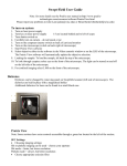
Photo: Ultima system without light box
Photo: Ultima IV (in vivo) without light box
Photo:Ultima system with light box and beam cover
5. Table Components
5.1 Lasers
Lasers
One of the major components of a multi-photon microscopy system is the laser. The laser used to create dual-photon excitation has a range from 700 – 1000 nm or
greater. For Ultima Systems with the AOD option, Prairie Technologies strongly recommends using a laser with pre-compensation.
Never look into the laser beam path! The lasers used with the Ultima system include Class 4, ultra-fast infrared (IR) lasers. These lasers do not have a beam visible
to the naked eye. The optics used in this system may cause back-scattered or reflected laser light. It is therefore critical to operate this system following all safety
instructions and wearing appropriate laser-safe eyewear.
5.2 Table Optics
Table Optics
Prairie Technologies provides the required table optics for the steering of an IR laser into the Ultima scanhead. We have stringent quality guidelines to provide the
customer with the best available products.
Our mirrors are specially coated to withstand high-powered IR light. Still, IR light will damage these mirrors over time. It is recommended to have your mirrors replaced
and table re-aligned every two years.
After exiting the laser cavity, the beam is usually sent to a zero-order half-wave plate. This, used in conjunction with a beam splitting cube, allows a selected amount of
laser light to be sent to one of two paths. For single scope setups, the second beam path is sent into a beam dump.
After being sent through a Pockels cell modulator, a pick-off mirror is placed in the path of the attenuated beam. This mirror sends approximately 2-5% of the beam
power to a power meter for monitoring purposes.
An interlocked electronic safety hard shutter is included in the beam path to prevent laser light from entering the scanhead when not imaging.
Never look into the laser beam path! The lasers used with the Ultima system include Class 4, ultra-fast infrared (IR) lasers. These lasers do not have a beam visible
to the naked eye. The optics used in this system may cause back-scattered or reflected laser light. It is therefore critical to operate this system following all safety
instructions and wearing appropriate laser-safe eyewear.
5.3 Pockels Cell
Pockels Cell
The Pockels cell is a delicate, consumable electro-optical device. The incorrect alignment of this component will cause it to fail. Do not adjust unless instructed to
by Prairie personnel.
The Pockels cell is a delicate, consumable electro-optical modulator used to attenuate the power of the laser to the scanhead. The voltage applied to the Pockels cell
is controlled through Prairie View. The base voltage (zero output) is set by adjusting the knob on the front of the Conoptics box. This number might change slightly
depending on wavelength, but should be within ±30.
The Pockels cell receives its signal from the Conoptics control box by two BNC cables, while the Conoptics box receives commands from the Device Controller via a
BNC connected to input J3.
To check the baseline voltage of the Conoptics box:
1. Align a bright sample in the field of view and set up scope for 2-photon imaging.
2. Set Pockels cell power to 0 in Prairie View.
3. Begin Livescan.
4. Set channel imaging color to Range Check.
5. Bring up PMT voltage until a light image of the sample can be discerned.
6. Adjust the black knob on the front of the Conoptics box to minimize the brightness of the sample. It may be necessary to increase the PMT voltage again.
7. Note the number displayed on the Conoptics box LED for the wavelength you are using.
If you find that you have to adjust the Conoptics box regularly or the base line number seems to be changing drastically, please contact Prairie.
6. Hardware and Electronics
6.1 Microscope
Microscope
The Ultima Multiphoton Microscopy System is built around a modified upright microscope. It can also be modified for use on an inverted microscope as well. The
manuals associated with this microscope have been provided to the user. Please refer to these manuals for specific information about the microscope components.
The Ultima In Vivo System is built on a fixed or moveable pillar platform. There is no standard transmitted light path or option for Dodt Gradient Contrast System.
6.2 Laser Light Path
Laser Light Path
After passing through the standard table optics and hard shutter, the beam passes into an enclosed beam-steering periscope assembly, which steers the aligned
beam into the sidecar. As it enters the sidecar, the beam passes through an alignment iris and into the scanhead (a self-contained unit not accessible to the user),
where it passes through one or more matched pairs of galvanometers, optics, and optical components suitable for raster scanning a microscope image when coupled
to an appropriate objective lens. The beam exits the objective and is scanned across the sample as a means of fluorescent excitation.
Figure: Ultima Scan Head Light Path
6.3 Dichroics
Dichroics
The Ultima has multiple mirrors/dichroics, as shown in the photo above. Some of these dichroics are fixed and others are user-changeable.
Image: Ultima Scan Head Dichroic Locations
?
Beam Combining Dichroic: The Beam Combining Dichroic is a 760nm dichroic used to combine the two 2-photon laser beams so one may be used to
image and the other to uncage. In single galvo systems this dichroic is not necessary.
?
Camera Port Mirror/Dichroic: A 100% mirror is supplied as standard equipment in the Camera Port Mirror/Dichroic position. The knob on the right hand side
of the scan head is used to move it in and out of position. When it is in position, the Ultima operates as a laser scanning system. When it is retracted, a normal
CCD camera (customer supplied) may be used with standard trans-illuminated or epi-illuminated microscopy techniques. This is not a user-changeable mirror.
It is possible to mount a dichroic mirror in this position. Contact Prairie for more details.
Note: The Camera Port mirror is not user-changeable. If you think something is wrong with your Camera Port mirror, please contact Prairie Technologies.
?
Primary Dichroic: The Primary Dichroic is located in the epi-fluorescence illuminator turret position one. Based on the specific system configuration selected,
this is a 660nm, 700 nm, or 720 nm LP dichroic. Additionally, there is a paired IR blocking filter located between the dichroic and the PMTs.
?
PMT Dichroic: The PMT Dichroic is the main user-changeable dichroic. It is based on a standard Olympus cube. For a dual detector system, this dichroic
includes a 575nm dcxr dichroic mirror and 607/45nm & 525/70nm barrier filters in front of PMT1 and 2 respectively. This combination was chosen to optimize
dual labeling using Alexa 594 and Alexa 488. If removed entirely, all light is sent to PMT 1.
For a quad detector system, there are two PMT dichroics. The standard cubes that come with a quad detector are selected at the time the system is ordered
and are designed to maximize the available wavelengths. To remove the PMT dichroics, pull down on the magnetic cover on the bottom of the housing.
Figure: Emission Light Path for Dual-Channel Detectors
Figure: Emission Light Path for Quad-Channel Detectors
6.4 Electronics Overview
Electronics Overview
The Ultima Multiphoton Microscopy System contains many electronic and optical components. In this section, the electrical rack and peripheral components will be
described.
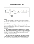
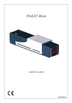
Image: Ultima Electronics Rack
The Ultima electronics rack contains the majority of electronics necessary to operate the Ultima system.
Monitors: Two flat-panel displays are standard with each system.
Workstation: Prairie Technologies provides a workstation to control the Ultima and its components and collect data. The workstation comes pre-loaded with all of the
cards, drivers and software necessary to control the Ultima system.
Device Controller: The device controller is the main communication device between the separate components.
Galvonometer Control: Each set of galvonometers has a separate control box on the electronics rack. See Galvos & AOD for more information.
BNC Breakout Boxes: The three BNC Breakout boxes associated with each system provide in/out triggers for imaging and synchronization. See NI Boards and Boxes
for more information.
PMT High Voltage Power Supply: Depending on the number of PMTs present on the system, there will be an HV box for each pair. See Detectors for more
information.
Pockels Cell Controller: For each modulated laser beam entering the Ultima, there is a corresponding pockels cell and control box. See Pockels Cell for more
information.
Main Rack Power Switch: All of the rack components are connected to a rack mounted, grounded power strip.
6.5 Detectors
Detectors
PMTs are extremely sensitive to light. Care should be taken to eliminate all sources of stray light from reaching the PMTs, as this will dramatically reduce the
sensitivity of the system. Prairie Technologies provides a light-tight and laser safe enclosure around the instrument to ensure optimal performance as well as to provide
a safe working environment for the users of this instrument.
The Ultima uses externally mounted, non-descanned side-on photomultiplier tube (PMT) detectors to collect the fluorescence emitted from the specimen. The
standard configuration for PMTs is a two channel, top-mounted detector setup. Most Ultimas can also be configured for four top-mounted PMTs and/or two sub-stage
PMTs.
Prairie offers two different types of PMTs: multi-alkali and GaAsP. The multi-alkali PMTs come standard and are side-on Hamamatsu PMTs hand-picked for their low
dark current. The GaAsP detectors are also Hamamatsu and are useful for applications requiring super-high sensitivity in the collection of data.
The multi-alkali PMTs have two cables attached. One connects to the high voltage box to receive the voltage applied to it, while the shorter cord sends the gathered
signal to the preamp. In addition to the high voltage cable and the signal cable, the GaAsP detectors also require a power cable to power the cooling fan.
Top-Mounted
The standard signal collection for an Ultima system comes from either a dual or quad top-mounted PMTs to the left of the epi-turret. The fluorescence from the sample
is transmitted through the objective lens, reflected off the primary dichroic, through the IR-blocking filter and through the various dichroics and barrier filters to the
PMTs.
Figure: Emission Light Path for Dual-Channel Detectors
Figure: Emission Light Path for Quad-Channel Detectors
Sub-Stage
An optional source of signal detection is from sub-stage detectors. Placed below the specimen, these detectors collect transmitted fluorescence and second-harmonic
generation signal.
To image with sub-stage detectors, move the two knobs in to the “Image” position (see below).
Image: Substage Detectors with mirror and shutter toggles labeled.
Protecting the PMTs: When the EPI light source is in use, the two knobs for the sub-stage detectors should be in the “Close” position (see above) to protect the PMT. If
the light from the illuminator is directed to the PMTs, they will be damaged and need replacing. This damage is not covered under warranty.
To achieve maximum intensity in sub-stage detectors, the condenser aperture should be in the open position and aligned for proper Köhler illumination.
Dodt Gradient Contrast
Prairie’s Dodt Gradient Contrast Imaging System is available as a secondary imaging system for the Ultima to help image unstained cells for electrophysiology
experiments such as patch-clamping. It uses transmitted light from an IR laser scan to create a DIC-like image. To collect this information, the Dodt tube and mirror are
placed in line between the scope condenser and the lamphouse. The mirror directs the signal to a PMT above the main housing. To prevent accidental over-load of the
PMT, an interlock is used to automatically shut off the lamphouse when the Dodt mirror is in the path.
Protecting the PMTs: When the EPI light source is in use, the Dodt mirror should be in the “out/off” position (under “misc” tab in PrairieView software) to protect the
PMT. If the light from the illuminator is directed to the PMT, it will be damaged and need replacing. This damage is not covered under warranty.
The Dodt aperture motor is controlled by an external control box, which includes a remote for the user to control the portion of light sent to the PMT. The Dodt mirror
and filter tray are controlled by the computer via a USB cable.
6.6 Dual Preamplifier & HV Control Unit
Dual Preamplifier & HV Control Unit
Figure: Dual Preamplifier & HV control unit
The PMT High Voltage (HV) is controlled via the PMT control unit mounted in the electronics rack. Each unit controls up to two PMTs.
The commands for the voltage are received by the HV box via the C.C. Inputs on the rear of the box. These commands come from the Device Control box. The signal
is sent to the PMTs by the BNCs attached to the HV Outputs on the rear of the box.
There are several controls on the front of the HV box. Included on the LED panel showing the HV output of the box is a dial. This dial is only to be used if the control
for that PMT is set to Manual. All HV boxes are factory set to Computer Control to be used in conjunction with the Prairie View software. The buttons located directly
below the LED displays are only used to calibrate the LED displays. They are factory set to display the correct high voltage values for each PMT but have no effect on
the voltage itself. Do not change these settings, as re-calibration is difficult and time-consuming.
The PMT HV control unit has overload protection circuitry designed to prevent damage to the PMTs caused by exposure to an overly bright light source. First is the
photodiode that is located in the PMT HV box. When the Sensor toggle is in the down position, the PMTs will be set to ~ 0 V if the room lights are turned on. If the
room lights are then switched off, the PMTs are turned back on. This mode of protection is only activated by external light sources.
The second protection is built in to the signal detection electronics. The switch in the center of the unit labeled Protect/Override is used to either enable this feature
(Protect mode) or disable it (Override mode). In Protect mode, when an excessively bright signal is detected by the PMT, the high voltage is set to 0 V.
Note: The LED display calibration buttons located directly below the LED displays should not be used. These controls are only used to calibrate the LED displays.
They are factory set to display the correct high voltage values for each PMT but have no effect on the voltage itself. Do not change these settings, as re-calibration is
difficult and time-consuming.
PMTs are extremely sensitive to light. Care should be taken to eliminate all sources of stray light that may reach the PMTs, as this will dramatically reduce the
sensitivity of the system. Prairie Technologies provides a light-tight and laser-safe enclosure around the instrument to ensure optimal performance as well as to provide
a safe working environment for the users of this instrument.
6.7 National Instruments Boards and Boxes
National Instruments Boards and Boxes
There are three National Instruments PCI boards in the system computer, the NI 6052E, NI 6713, and the NI 6110 or 6115. These boards control the three external,
rack-mounted National Instruments BNC breakout boxes, two 2090 units and one 2110. The upper 2090 box is referred to 2090A and the lower is referred to as 2090B.
All of the NI boards and boxes are connected through the PFI0/Trig1 channels to synchronize the experiment/acquisition start triggers among the three NI boards.
NI 6110/6115 Board and BNC 2090B Box
The 6110 or 6115 card is responsible for the creation of the imaging output waveforms and collecting the signals from the PMTs. The 6110 card is used for regular
galvo-only imaging systems, while the 6115 card is used for the high-speed imaging AOD. The 6110 board samples at 2.5 million samples per second and allows
dwell times in multiples of .4µs. The 6115 board samples at 10 million samples per second and allows dwell times in multiples of .1µs.
The output waveforms for the imaging galvos, are output on the 2090B’s DAC 0 Out and DAC 1 Out. The 2090B box also provides the input for the PMT data on BNCs
ACH 0 – 3. These four channels correspond to four high-speed ADC 12-bit input channels on the 6110 or 6115 board.
NI 6052E Board and BNC 2090A Box
The NI 6052E board collects all the input signals generated while running an experiment. These input signals are collected by the 2090A box at BNCs ACH0 – 7. They
are represented in the software as the eight TriggerSync acquisition channels. The maximum sampling rate for this board can be as high as 333K samples/sec. For
each additional channel enabled, the maximum sampling rate is proportionally decreased.
Figure: NI BNC-2090 boxes A (top) & B (bottom)
Figure: Close-up of NI BNC-2090 boxes
NI 6713 Board and BNC 2110 Box
The NI 6713 board generates the output waveforms for the uncaging galvos, the Pockels cell, and the stimulus signals available in TriggerSync for use in experiments.
This board can generate a waveform at 1M samples/sec if only one channel is enabled. The maximum sampling rate drops as more channels are enabled. DAC5OUT
and DAC7OUT are set aside for driving the uncaging galvos. DAC0OUT-DAC4OUT and DAC6OUT are available through TriggerSync for other experiments.
Figure: NI BNC-2110
# of Channels
1
Max Input Samples/Sec for NI 6052
333K 166K 111K 83K
2
3
4
Max Output Samples/Sec for NI 6713
1M
5
6
7
8
67K
56K
48K
42K
500K 333K 250K 200K 167K 143K 125K
Table: Maximum NI-6052 and NI-6713 sample rates
Software Communication Through NI Hardware
The software used for imaging, Prairie View, and the triggering software, TriggerSync, communicate by passing messages to each other using a TCP/IP protocol. In
order for Prairie View to recognize that TriggerSync is running, TriggerSync must be started (or restarted) after Prairie View is in operation. Hardware synchronization
of image collection and electrical recording is achieved by sharing a TTL trigger signal by the 6052, 6110, and 6713 boards (the PFI0/TRIG1 input on the upper
BNC-2090, lower BNC-2090, and BNC-2110 box for the 6052, 6110, and 6713 boards, respectively). Prairie View and TriggerSync are triggered by a falling edge on
PFIO/TRIG1.
6.8 Device Control Box
Device Control Box
The Device Control Box contains power supplies, motor drivers, and the logic for responding to commands from the RS-232 computer input or the DCRI.
Cables from the back of the Device Control Box go to many of the other boxes on the electronics rack. Three LEDs on the front of the Device Control Box provide basic
status information. The leftmost LED indicates power on, the center LED is on whenever the controller has moved any of its three motors within the previous half
second. The rightmost LED indicates the status of the RS-232 send and receive lines. Traffic through the RS-232 port causes very brief, dim flashes on this LED. This
LED will flash continuously 10 times per second if an RS-232 transmission error causes the input command buffer of the controller to overflow. In this state no further
commands are recognized by the Device Control Box, the motors will halt, and the controller must be reset by either cycling power or pressing the reset button located
on the front of the Device Control Box.
6.9 Device Control Remote Interface (DCRI)
Device Control Remote Interface (DCRI)
To provide easy access to x, y and z motor control, Prairie provides a Device Control Remote Interface (DCRI) box. The motor system consists of the Prairie Device
Control Box, the DCRI, an RS-232 cable, the motorized stage and a z-motor. The DCRI box has a knob for each motor x, y and z, and a series of toggles to control
table components and motor movement. The Coarse/Fine and Normal/Alt toggles affect the movement of the motors when controlled with the knobs. Coarse/Fine will
switch the motor between a coarse movement of approximately 31um per knob turn versus a fine movement of 1.95 um per knob turn. For all axes, the amount of
motion for a single motor step is an ideal estimate. The actual amount of motion will vary due to internal factors within the motor, drive electronics inaccuracies, and
friction within the mechanical hardware.
The Normal/Alt toggle controls when the motors are enabled. In Normal mode each motor individually disables itself after its most recent motion, and enables itself
immediately before being ordered to move. When disabled, the motors do not resist being turned by hand and will not hold the stage stationary if other disturbances
occur. In Alt mode the motor is enabled continually whether or not it is moving, keeping the stage stationary, but possibly introducing noise into the image signal.
Axis
X
Y
Z
Coarse Mode
Fine Mode
312.5 µm
19.5 µm
312.5 µm
19.5 µm
31.25 µm
1.95 µm
Table: Motor controller resolution
6.10 Preamplifier
Preamplifier
The Prairie Preamplifier receives the signal from the PMTs and amplifies it before sending it to the input channels on the 2090B box. It is powered by the High Voltage
Box and controlled by the computer via a USB cable.
The preamplifier can receive input on up to four channels. Each preamplifier channel (also referred to as a blade) can receive two inputs, a main and a secondary
PMT. If only one PMT signal is to be received for each channel, the left BNC input is used. The right BNC is used when averaging in a second PMT signal such as
from a sub-stage detector.
6.11 Galvos & AOD
Galvos & AOD
The Prairie Galvanometer Control Box controls a set of galvonometers carefully tuned for best performance. Damage can occur if the galvos are run with the wrong
drivers.
Caution: Switching cables so that the drivers control the wrong galvos can cause galvo damage.
In systems with a single galvo pair used for both scanning and uncaging, the scanning inputs are connected to the 'X Input' and 'Y Input' BNC connectors and the
uncaging inputs are connected to the 'X2 Input' and 'Y2 Input' BNC connectors. The 'Switch' BNC input is driven by TriggerSync to select between the scanning and
uncaging control signals.
In systems with separate pairs of galvos for scanning and uncaging, each pair uses the 'X Input' and 'Y Input' signals from its own galvanometer control box.
Two amber-colored LEDs on the front of each box illuminate to indicate a shutdown state for the X and Y galvos, which occurs briefly on power up an afterwards only if
the galvo experiences some failure such as being driven too hard so that it overheats. The 'X Feedback' and 'Y Feedback' are galvo position feedback signals which
are used by Prairie during testing and configuration.
AOD
An alternative laser scanning system for video-rate imaging of specimens is available for the Ultima. This system makes use of an acousto-optic deflector to create the
x raster scan of an image. AOD systems will use the same Galvanometer Control Box as standard imaging systems. In AOD scanning mode the X galvo is held still
and used for panning the image while the AOD scans in X.
6.12 Piezoelectric Z Device
Piezoelectric Z Device
Piezo Controller
This specially modified piezoelectric controller allows for up to 460um of high-sensitivity travel for high speed Z-series acquisitions.There are two modes of operation
for the piezo. With the Servo switch set to on, the piezo works in closed-loop mode, with 400 µm of travel in closed loop mode. When the Servo switch is set to off, the
piezo runs on open loop mode with a maximum travel of 460 µm.
When used with PrairieView, the current position (offset) of the piezo, regardless of the state of the switch (ANALOG/DIGITAL), will always be shown. When this switch
is in the ‘ANALOG’ setting, the position of the piezo is controlled via the ‘DC-OFFSET’ knob on the E-665 controller. Any movement commands from Prairie View will
be ignored. When this switch is in the ‘DIGITAL’ setting, the ‘VOLTS’ and ‘MICRONS’ display on the controller will go blank and the ‘DC-OFFSET’ know will no longer
affect the piezo position and now movement commands from PrairieView will be executed.
To take advantage of the higher speed acquisition capabilities of the piezo controller (selected by checking the Fastest Acquisition check box on the Z-Series tab
(only available when the Z-Series device is the E-665 piezo controller) requires an input trigger to control the stepping of the piezo controller:
Ø
Typically this signal will be the ‘End of Frame’ trigger.
Ø
The trigger signal is configured via the ‘File’ menu option, then select the ‘Preferences’ option, and then select the ‘Output Trigger Type’ option.
Ø
This signal is found at the ‘PFI8’ connector on the BNC-2090A box (connected to the PCI-6052E NI DAQ card).
Ø
The software configuration and necessary wiring information is provided in the trigger signals section.
Ø
This trigger signal is input to the E-665 on the ‘I/O Connector’ on the back of the controller via pin 9 (this is a DB-9 connector).
7. Ultima Quick Start
Ultima Quick Start
1. Turn on the main power switch at the rack.
2. Following instructions from laser manufacturer, put laser in “on” or “ready” state.
3. Check and/or install the filters and dichroics into the upper PMT detection path.
4. Turn on the PC (Note: Disable anti-virus software).
5. Start PrairieView.
6. Start TriggerSync if you plan to conduct electrical recording experiments.
7. Verify the communication link between Prairie View and TriggerSync. A message will appear at the bottom of the Prairie View window stating that the link has been
established.
8. Push the trinoc plunger in to the ‘Bi’ position.
9. Position the epi-dichroic wheel to an open position. (Transmitted light will turn on automatically.)
10.
11.
Put sample on stage and focus through the binoculars.
Make sure the epi-fluorescence mercury lamp is completely shuttered or off if present on your system. The shutter mechanism provided on the front of the
epi-fluorescence illuminator is NOT an adequate shutter, as it leaks light from the lamp house that will flood the PMTs.
12.
Turn the epi-dichroic wheel to position ‘1’ (This automatically turns off the transmitted light source, and directs signal to the upper PMTs.)
13.
Pull the trinoc plunger out to the ‘LSM’ position.
14.
Close light box door.
15.
Turn off the room lights.
16.
Open the laser’s hard shutter in PrairieView or the laser manufacturer’s software.
17.
Press Live Scan. This starts the scanning, and opens the laser path hard shutter.
18.
In the Laser, PMT, DAQ tab, bring the PMT high voltage up to mid-range, about 500 – 600 depending on the laser and PMT type.
19.
Increase the Pockels cell percentage until an image is visible. This should be about 2-5%.
8. Ultima IV Quick Start
Ultima IV Quick Start
1. Turn on the main power switch at the rack.
2. Following instructions from laser manufacturer, put laser in “on” or “ready” state.
3. Check and/or install the filters and dichroics into the upper PMT detection path.
4. Turn on the PC (Note: Disable anti-virus software).
5. Start PrairieView.
6. Start TriggerSync if you plan to conduct electrical recording experiments.
7. Verify the communication link between PrairieView and TriggerSync. A message will appear at the bottom of the PrairieView window stating that the link has been
established.
8. Turn on the epi-fluorescence mercury lamp to warm up.
9. Push the trinoc plunger in to the ‘Bi’ position.
10.
Position the epi-dichroic wheel to an epi-cube appropriate for the sample.
11.
Put sample under the objective.
12.
Open the turret's back shutter.
13.
Turn up mercury lamp power.
14.
Focus on specimen.
15.
Turn off or COMPLETELY shutter the epi-fluorescence mercury lamp house if present on your system. The shutter mechanism provided on the front of the
epi-fluorescence illuminator is NOT an adequate shutter, as it leaks light from the lamp house that will flood the PMTs.
16.
Turn the epi-dichroic wheel to position ‘1.’
17.
Pull the trinoc plunger out to the ‘LSM’ position.
18.
Close light box door.
19.
Turn off the room lights.
20.
Open the laser’s hard shutter in PrairieView or the laser manufacturer’s software.
21.
Press Live Scan. This starts the scanning, and opens the laser path hard shutter.
22.
In the Laser, PMT, DAQ tab, bring the PMT high voltage up to mid-range, about 500 – 600 depending on the laser and PMT type.
23. Increase the Pockels cell percentage until an image is visible. This should be about 2-5%.
9. Alignment & Calibration
9.1 Beam Alignment
Beam Alignment
Important: The optical path for the laser beam has been carefully and precisely aligned. Re-aligning the laser beam may be necessary only under the following
circumstances and should be performed only by a factory-trained and authorized technician:
·
The direction of the laser beam out of the laser cavity changes.
·
A mirror on the tabletop is adjusted.
·
A Pockels cell is added to or removed from the light path.
·
Something new is added to the light path that would cause the direction of the beam entering the Ultima to change.
Never look into the laser beam path! The lasers used with the Ultima system include Class 4, ultra-fast infrared (IR) lasers. These lasers do not have a beam visible
to the naked eye. The optics used in this system may cause back-scattered or reflected laser light. It is therefore critical to operate this system following all safety
instructions and wearing appropriate laser-safe eyewear.
9.2 Scan Head Alignment
9.2.1 Imaging Beam Alignment
Imaging Beam Alignment
Important: Re-aligning the imaging laser will introduce an offset into all of the spot calibration files.
1. Close PrairieView.
2. Close TriggerSync.
3. Remove sample.
4. Raise objective lens all the way up.
5. Install objective target in turret.
6. Open National Instrument's Measurement and Automation.
a
b
c
d
e
f
7. Open
Select Devices and Interfaces.
Select Traditional NI-DAQ devices.
Select PCI-6110.
Select Test Panels.
Use analog output and DC voltage.
Set channels 0 and 1 to 0.00 Volts. Be sure to press update channel after selecting each channel.
shutter for imaging beam.
8. Verify that the image of the X-axis galvo mirror is centered on objective target.
9. Insert sidecar fluorescent target.
10.
Use adjustments at the sidecar turning mirror to center beam at the sidecar target.
11.
Remove sidecar fluorescent target.
12.
Use adjustments on the front sidecar mirror to center beam on objective target.
13.
Repeat the two sidecar adjustments until the beam is centered on both targets.
14.
Stop iris down only to the size of the ring in the objective target window.
15.
Leave iris in this position to minimize back reflections into upper PMTs.
16.
Close measurement and automation.
17.
Close imaging beam shutter.
18.
Restart system software.
9.2.2 Uncaging Beam Alignment
Uncaging Beam Alignment
Important: Re-aligning the uncaging laser will introduce an offset into all of the spot calibration files.
1. Close PrairieView.
2. Close TriggerSync.
3. Remove sample.
4. Raise objective lens all the way up.
5. Install objective target in turret.
6. Open National Instrument's Measurement and Automation.
a Select Devices and Interfaces.
b Select Traditional NI-DAQ devices.
c Select PCI-6713.
d Select Test Panels.
e Use analog output and DC voltage.
f Set channels 5 and 7 to 0.00 Volts.
g Be sure to press update channel after selecting each channel.
7. Open shutter for uncaging beam.
8. Verify that the image of the X-axis galvo mirror is centered on objective target ring.
9. Insert sidecar fluorescent target.
10.
Use adjustments at the sidecar turning mirror to center beam at the sidecar target.
11.
Remove sidecar fluorescent target.
12.
Use adjustments on the front sidecar mirror to center beam on objective target.
13.
Repeat the two sidecar adjustments until the beam is centered on both targets.
14.
Stop iris down only to the size of the ring on the objective target.
15.
Leave iris in this position to minimize back reflections into upper PMTs.
16.
Close measurement and automation.
17.
Close uncaging beam shutter.
18.
Restart system software.
9.3 Spot Detector Alignment
Spot Detector Alignment
Important: This is normally a one-time adjustment. The only time this will need to be performed is if either galvo is replaced, a mirror in the scan head is moved, or the
beam combining dichroic in the scan head is replaced.
1. Put reflective chrome slide on stage.
2. Start PrairieView.
3. Enable Channel 1 in the Image Window.
4. Start TriggerSync.
5. Verify the communication link between PrairieView and TriggerSync. A message will appear at the bottom of the PrairieView window stating that the link has
been established.
6. Close uncaging shutter in the TriggerSync Mark Points window.
7. Image the slide with imaging beam.
8. Activate mark points screen. Make sure image in mark points screen is updating.
9. Manually toggle shutter on uncaging beam to burn small spot on chrome slide.
10.
Put red TriggerSync cursor over mark on chrome slide. (Do not use Nudge.)
11.
Turn off Channel 1 and turn on Channel 3.
12.
Close the hard shutter in the Ultima scanhead.
13.
Open uncaging shutter in TriggerSync.
14.
Activate focus.
15.
Move uncaging spot to be coincident to red TriggerSync cursor.
16.
Close uncaging shutter in TriggerSync.
17.
Open the hard shutter in the Ultima scanhead.
18.
Turn off Channel 3 and turn on Channel 1.
9.4 Calibrate Point Image
Calibrate Point Image
Important: Each objective lens will require its own unique calibration file.
1. Confirm imaging beam shutter is closed.
2. Start PrairieView.
3. Start TriggerSync.
4. Verify the communication link between PrairieView and TriggerSync. A message will appear at the bottom of the PrairieView window stating that the link has
been established.
5. Turn off Channels 1 & 2.
6. Turn on Channel 3.
7. Set to 4ms/line.
8. Open Uncaging laser shutter in TriggerSync.
9. Perform Point Calibration as described here.
9.5 Resetting the PMT High Voltage
Resetting the PMT High Voltage
Important: The PMT high voltage will automatically turn off if an overload condition is detected.
The system is designed with two levels of PMT protection. First is the photodiode that is located in the PMT high voltage power supply. This senses when the room
lights are on and automatically turns the PMT high voltage to 0 V. The second protection is built in to the signal detection electronics. When and excessively bright
signal is detected the PMT high voltage is again set to 0 V.
To reset the PMT high voltage power supply:
1. Correct the condition that caused the overload condition to occur. i.e. turn off room lights or close turret shutter.
2. Turn the Protect/Override toggle on the front of the PMT high voltage power supply momentarily to Override.
3. Turn the Protect/Override toggle on the front of the PMT high voltage power supply back to Protect.
This will cause the PMT high voltage power supply to return to its pre-overload values.
Important: When an image is not visible (or suddenly disappears), it may be due to this PMT HV safety feature.
10. PrairieView Software
10.1 Overview
Overview
PrairieView is the software that controls all of the scanning and image collection functions of the Ultima. Image size, scan rate, pan, zoom, PMT settings, laser
wavelength and power level, file saving and naming are all set and easily controlled using PrairieView. This acquisition software also offers a number of features to
meet most imaging needs including scan rotation, linescan, brightness-over-time (BOT), region of interest (ROI), z-series, photoactivation, marked points and T-series.
10.2 Main Window
10.2.1 Overview
Overview
Most of the controls of PrairieView are accessed through the Main Control Window. Some sections have extra controls accessible through a green bar located to the
left of the section, such as the image size section. Selected buttons are highlighted with a light orange outline on the button.
Screen Shot: PrairieView's main window.
10.2.2 Tear-Off Panels
Tear-Off Panels
As of Prairie View 4.0.0.0, certain panels may be "torn off" and placed on the user's desktop.
To tear off a tab, click on the diagonal arrow button located on the right side of the tab label. Prairie View will remember these selections and return the tear-off panels
to their last location when Prairie View is restarted. To return a tear-off panel to its original location, click the "X" in the upper-right corner.
Screen Shots: Lasers tab with tear-off option (left), Lasers tab tear-off with revert location option (right)
10.2.3 Image Size Controls
Image Size Controls
Screen Shot: Scan Resolution Tools - Standard
Image Size
Image size is a definition of how the collected data is acquired (and displayed). In the case of 512 x 512, data is acquired at 512 bins in x by 512 bins in y, with each
bin sampled according to dwell time. All images are collected at 72 pixels per inch.
Image Window Size
There are four options under Image Window Size:
·
Fit is the default and the image is shown as 512 x 512 pixels. If the image window is increased or decreased in size, the display will be scaled to fit
proportionally to fit in the new window.
·
1:1 shows the image at its actual size as defined by the Image Size.
·
Smaller decreases the image by ~10%. The image can continue to be reduced by clicking Smaller repeatedly.
·
Larger increases the image size by ~10%. The image can continue to be increased by clicking Larger repeatedly.
Pixels Per Line & Lines Per Frame
Screen Shot: Scan Resolution Tools - Custom
The Pixels Per Line and Lines Per Frame functions allow the user to define a rectangular scan pattern, where the number of rows of x is not equal to the number of
columns in y. Preset values are offered as a convenience. Values may also be selected by means of the slider tool or by typing directly into the highlighted field.
Pixels Per Line will set the number of pixels in a single scan line (x). The minimum value allowed is displayed to the left of the highlighted field.
Lines Per Frame sets the number of lines (y) per image.
Note: Be aware that it is possible to choose configurations in which the pixels are not square. This may effect how the images are displayed by third party software.
10.2.4 Dwell Time Per Pixel
Dwell Time Per Pixel
Screen Shot: Dwell Time Per Pixel Controls
Controls the dwell time that the laser beam is at each pixel location in the image, with values in microseconds (µs). The minimum value allowed is displayed below and
to the left of the slider. The current dwell time is shown to the right of the minimum. Increasing pixels per line, zooming or rotating may increase the minimum dwell
time possible.
Averaging/Summing
During data acquisition, the underlying sampling rate is 1 sample per 0.4 µs for a galvo-imaging system. This means that for a 4 µs dwell time, the system is either
averaging or summing 4 µs/0.4 µs =10 samples per bin.
10.2.5 Optical Zoom
Optical Zoom [mag]
Screen Shot: Optical Zoom Controls
Controls the size of the area of the specimen that is being scanned. An optical zoom of 2 will cause the microscope to scan an area that is ½ the width and ½ the
height of a scan at a zoom of 1. Optical Zoom does not affect the number of pixels in the image. It is possible to increase the true optical resolution of the system by
using this function. Selecting Reset will cause the zoom to return to the default value of 1. The minimum value allowed is displayed below and to the left of the slider.
The current selected zoom is shown to the right of the minimum.
Note: It is not possible to set the optical zoom to less than 1.
10.2.6 Scanning Controls
Scanning Controls
Screen Shot: Scanning Controls
Live Scan
To start the Ultima scanning, click on Live Scan. During a live scan, this button changes to read Stop Scan. Clicking it a second time causes the scan to stop and the
laser beam to be shuttered so that it no longer scans across the specimen. Only the last image of a Live Scan can be saved.
Single Scan
When Single Scan is selected, one image is acquired, with the result displayed in the image window(s). The laser is shuttered following collection of the image and
the image is saved as a temporary file. If Average Every N Frames is set to a number more than one, the selected number of frames will be acquired and averaged to
create one image.
New Window
Selecting New Window will cause another image window to appear on the desktop. It is possible to have multiple image windows open at one time. The operator can,
for example, assign a different PMT to separate image windows if desired.
Running Frame Average
The Running Frame Average affects the Live Scan imaging. When this option is checked, the software will average every chosen number of frames during Live
Scan and update the Image Window accordingly. This is useful for samples with little fluorescence or when using low laser power.
Average Every N Frames
Average Every N Frames is designed to work with the Single Scan command. When set to a number greater than one, it will average the selected number of frames
to create a Single Scan image.
Shutter Controls
There are two different table shutters used when imaging. The Hard Shutter is a physical shutter placed on the table. The Soft Shutter controls the bias applied to
the pockels cell.
The Hard Shutter automatically opens whenever an acquisition begins. Although software controlled for routine imaging, it is possible to manually open and close the
hard shutter to allow access to the beam by TriggerSync or other interfaced applications by clicking Hard Shutter Open or Closed.
It is also possible to manually open and close the Soft Shutter. This is most useful when the mechanical movement of the hard shutter causes disruptive vibration
during electrophysiological experiments. This can be controlled by clicking Soft Shutter Open or Closed.
Scan Mode: Galvo or AOD
AOD is Acoustic Optic Deflection which can provide up to 25 frames per second for a 512by 512 image. It is option and not available on all systems. The Scan Mode
button should be enabled if the system has AOD option. To switch between the standard galvo-driven imaging mode and the AOD driven imaging mode, click the
Scan Mode button.
See also:
AOD Mode.
Label Selection
Label Select allows the user to select previously defined and saved experimental protocols from a pull-down menu. These protocols include saved settings for active
channels, PMT selection and DAQ gain, laser power settings. Setting up labels is covered here.
Objective Lens
Objective Lens allows the user to select a previously calibrated objective setting for an objective used on the system. The procedure for calibrating objective lenses
can be found here.
Note: Proper objection selection is important as it is used in determining pixel size. Failure to select or use a properly calibrated objective will result in invalid
measurements.
10.2.7 AOD Mode
AOD Mode
Switching between galvo and AOD modes
Scanning Controls with AOD selected
In the Prairie View Scanning menu, click on Scan Mode to choose AOD. If the AOD is not connected or functioning, this box will be grayed out.
Differences between galvo mode and AOD mode
The Acousto-Optic Deflector (AOD) mode is capable of scanning at a much higher frame rate (25 frames per second/FPS) than galvo mode. Its speed makes it ideal
for capturing momentary phenomena that galvanometers cannot, such as dendritic spikes.
AOD mode also has a faster minimum dwell time (.1 compared to galvo mode's .4), which reduces photobleaching. However, the optical zoom, image size, and dwell
time are more restricted due to the current limitations of AOD technology.
Working with AOD mode
Frame rate (FPS) is determined by the image size, dwell time, and optical zoom settings.
Default AOD settings:
512 x 512 pixels
.1 dwell time
1.0 optical zoom
25 FPS
Note: Changes in any of these settings will cause Prairie View to automatically compensate by changing the others. This keeps the AOD calibrated correctly.
To select one parameter to keep constant, click the checkbox next to it. Prairie View will not change that setting unless you uncheck the box or restart Prairie View.
Frame Rate
Frame rate is calculated automatically based on the image size, dwell time, and optical zoom settings. For faster frame rates, set those parameters lower.
Image Size
The number of pixels in the scan area. Set higher for cleaner images, lower for faster frame rates.
Optical Zoom
This setting is separate from the zoom in/out feature in the image window. Zooming in/out in the image window does not change scan parameters.
Setting optical zoom to 4.0 allows the greatest range of image sizes and dwell times.
To get the full field of view, make sure the plunger position inside the AOD matches the optical zoom level. (If you do not know what the plunger position is, restart
Prairie View. The software will automatically detect the correct optical zoom. All other parameters will reset to default.)
Dwell Time
The amount of time spent imaging each individual pixel. Decrease to reduce photobleaching. The minimum possible setting in AOD mode is .1.
Each .1 change in dwell time increases/decreases optical zoom by 1.0 (e.g. 2.0 to 3.0).
Additional Tips
Increase image resolution by increasing either image size (total number of pixels) or dwell time (amount of time spent imaging each pixel). Note that changing either of
these settings will cause the optical zoom and frame rate to change accordingly.
Improve image quality with the Average Every N Frames feature. Because AOD mode scans so quickly, it can average frames much faster than galvo mode.
10.2.8 Pan & Scan Rotation Controls
Pan & Scan Rotation Controls
Screen Shot: Panning and Scan Rotation Controls
Pan Control
On the left is an indicator that shows the relative position and orientation of the scanned area. A red and yellow box indicates the scanned area; the yellow side is by
definition the “top” side. This box will change its size as a result of the Optical Zoom function described here. Similar changes will be displayed when the image is
panned, or shifted laterally, and when the scan is rotated.
Coarse/Medium/Fine controls the feel or resolution of the pan controls.
The image may be panned left, right, up, or down. To do so, click on the arrow indicating the direction to pan the image. Clicking 0 causes the pan to reset to the
middle of the field of view.
Scan Rotation
Scan rotation is controlled by means of the slider, or values (in degrees) may be typed directly into the highlighted field. Rotation is possible from -180° to +180°. Zero
will set the angle of rotation back to zero.
10.2.9 Stage Controls
Stage Controls
The stage controls allows the user to move the stage in the x, y, and z directions. It also allows the user to recall saved locations. The step size is shown to the left of
the movement buttons and has a default of 10 µm. Saved locations can be modified on the XY-Stage tab.
Screen Shot: Stage Controls
XY Stage Control
The XY stage controls allow the user to scan through the x and y axes of an image in user-define step sizes.
Use the arrow buttons to move the stage by the number of µm indicated in the XY Step Size field. To change the step size, click in the field and replace the number
with the desired step size.
Use the home feature to store an XY location to come back to at a later time. Selecting Set stores the current XY location as home and pressing the
return to that position.
button will
Select 0 to leave the motor where it is and set the current position to be zero.
Z-Motor Control
The z-motor controls allow the user to scan through the z-axis of an image in user-define step sizes.
Use the
and
arrows to move the z-motor by the number of µm indicated in the Z Step Size field. To change the step size, click in the field and replace the
number with the desired step size.
Use the home feature to store a Z location to come back to at a later time. Selecting Set stores the current Z location as home and pressing
position.
Select 0 to leave the motor where it is and set the current position to be zero.
will return to that
Z Devices
If there is more than one z device available on the system, such as a high-precision piezo controller, this control will be active to select which device to control. More
information about the piezo controller z-device can be found here.
10.2.10 Laser, PMT, DAQ Tab
Laser, PMT, DAQ Tab
The Laser, PMT, DAQ tab is separated into three separate sections. The Pockels cell throughput (laser power at the sample) is controlled on the left-hand side while
the PMTs and preamplifier settings are controlled on the right. The PMT controls are on the front panel while the preamplifier controls can be accessed by selecting
the green bar in the center of the tab.
In Prairie View 4.x, this tab and others may be torn off and placed on the user's desktop.
Screen Shot: Laser Controls
The laser sliders are used to adjust the laser intensity that reaches the specimen. In most Utima systems the imaging beam intensity is controlled via a Pockels cell
that is tied to this control. If your system has two lasers then a second slider will be activated to control a second Pockels cell for the uncaging laser intensity.
If there is a laser launch associated with the system, the laser line powers will also be accessed through this panel.
Which controls are visible for each laser depends on system configuration and calibration. See calibrating laser power.
Check Interlaced scan pattern to enable interlaced scanning mode. See interlaced scanning.
Screen Shot: PMT Controls
The PMT HV controls the voltage which amplifies the photon-electron signal-to-current pulse. Increasing the PMT HV will increase the output current pulse and thus
increase the brightness of image. To reset all PMTs’ voltages to zero, click Zero next to PMT Master. To adjust individual PMT voltage, slide the slider bar or click the
arrows under that PMT HV.
The text field to the right displays the voltage that corresponds to the red LED displays on the Dual Preamplifier & HV Control Unit in the instrument rack. Clicking
Zero at the end of a PMT HV slider sets that PMT HV to zero.
Screen Shot: Preamp Controls
To modify a preamplifier setting, first use the Channel Selection pull-down box to select the channel to change the control setting for. Then use the Gain and Offset
controls to modify the desired parameter.
The Filter Bank control affects collection rate of the channel.
Note: When you change the Filter Bank value for one channel, it will change the filter bank selection for all channels.
Screen Shot: DAQ Controls
DAQ is an abbreviation for data acquisition, which samples the photo-electric signal from the PMT to generate an image that can be manipulated by the data
acquisition board (the NI DAQ 6110 board). The function of DAQ is to scale the amplified photo-electric signal to match the acceptable input range of the data
acquisition board) for maximum image resolution.
The acceptable input range for the data acquisition board is fixed (from -10v to +10v). Because the dynamic photon signal from the preamplifier may be greater or less
than the selected range, adjusting the DAQs, the dynamic photon signal will be scaled to the data acquisition board’s range to achieve best image resolution. DAQs
values are preset in drop-down list. To change the DAQs, click the drop down arrow and select the value from the dropdown list. The higher the DAQs, the narrower
the input range and the higher the image contrast.
Note: Adjusting DAQs does NOT change the signal from the detector and preamplifier. Setting the DAQs to an in-compatible range may result in real signal being lost.
10.2.11 Interlaced Scanning
Interlaced Scanning
Screen Shot: Interlaced Scanning Setup Dialog
Interlaced scan patterns allow acquisition of frames using up to four different independent laser settings alternating each line for higher temporal resolution than is
possible with using labels to alternate settings each frame. One line of each track is scanned to acquire one line of the final image.
Note: While this feature is available for systems with only a single laser, its usefulness with a single laser setup is limited at best. This feature is primarily useful when a
system has more than one laser (either 1-P or 2-P).
For example, if a system has two imaging lasers: one tuned to 800 nm and one tuned to 900 nm this feature allows the operator to scan a 512x512 image alternating
wavelength with each line. The data for track one will be saved as the Channel One data and the track two data will be saved as channel two.
Whenever the Interlaced scan pattern check box is checked, the defined interlaced settings will be used. This applies to Live Scan, Single Scan, T-Series, Z-Series,
etc.
Laser Selection
Specifies one of the lasers currently configured on the system as well as a power setting. The laser and power here can be added directly to an active track. By default
the current power check box is checked which indicates that the current power setting should be used even as the current value changes. When unchecked a static
power value can be specified.
Tracks
A Track is a sequence of laser lines and powers to control. Up to four different Tracks may be defined.
There is a check box on the left of each track to enable it. Once enabled it is possible to add the selected laser and power to it using the
can be used to update the power setting from a laser already added to the track. To remove a laser from a track press the
button. The same button
button. Any lasers not included in a
track will be turned off.
Channel Mapping
During each track there are four possible channels to be acquired; multiply that by the four tracks and there are sixteen possible data sources which need to be
mapped to the four data channels. To do this each display channel has a source channel and source track associated with it.
For example channel one could get its data from channel one of track one and channel two could get its data from channel one also, but channel one of track two.
10.2.12 Z-Series Tab
Z-Series Tab
The Z-series tab contains the controls used to collect stacks of images called Z-Series or Z-Stacks. This tab allows the user to define start and stop positions, step size
or number of steps and necessary laser power adjustments.
In Prairie View 4.x, this tab and others may be torn off and placed on the user's desktop.
Screen Shot: Z-Series Tab
Z-Series Calculator
In order to collect a Z-Series stack the operator must define several parameters that define the range, resolution, and signal levels. Four values are needed to define
the range and resolution of a Z-series: Start Position, Stop Position, Step Size, and Number of Slices or image planes. By entering values for any three of these
values, the fourth value will be calculated automatically. The Define/Calculate radio buttons indicate the three values that the operator must define as well as the one
that is calculated by the system.
Laser Power Gradient
The Laser Power Gradient control affects the way Pockels cell power is controlled throughout a Z-Series. When Adjust Laser &PMT is checked, the Laser power
Gradient control is active. This pull down menu allows the user to specify the laser control that the gradient control operation will be applied to. This is only active if
there is more than one imaging laser. The settings are retained for each Z-Series definition and each saved z-series can have a different gradient setting. There is also
a check-box to allow the settings to be applied to all imaging lasers.
The user can choose the equation applied to the Pockels cell power by selecting Default or Custom. The Default gradient is a slight parabola defined by Prairie View.
Custom allows the user to enter their own gradient line for the acquisition. The user can enter a number in the field to the right of Custom or select graph. If graph is
selected, a dialog will appear for viewing the custom gradient versus the default. There may be additional lines for other imaging lasers.
Screen Shot: Custom Laser Gradient Dialog
The x-axis (horizontal) of the graph represents the z position of the current Z-Series while the y-axis (vertical) of the graph indicates the laser power/setting as a
function of the z position. As the Adjust Gradient slider is moved, the graph will automatically update with the new relationship between the laser power and z
position. In addition, the operator may type in a Gradient value in the text box located below the Adjust Gradient slider.
If more than one imaging laser is present, then the operator may click on the Show All Lasers check box to display the graphs of all laser powers as a function of z
position for the current Z-Series definition.
Selecting Cancel, will dismiss any changes made to the gradient with the graph and close the dialog.
If the operator chooses Accept, the new gradient setting will be applied to the selected laser line(s). This will be shown by the updating of the value in the Custom
field to reflect the changes made in the graph.
Triggered Z-Series
If No Input Trigger for Z-Series is selected, then the Z-Series will start immediately when the Start Z-Series button is pressed.
If Start Z-Series with Input Trigger is selected, then after Start Z-Series is pressed, the z-motor will move to the position of the first slice/image, the laser and/or PMT
settings will be set, the hard shutter will open, and the software will wait for the arrival of an external input trigger before acquiring the first slice/image. After that, all
subsequent slices/images are acquired automatically.
If Use Input Trigger for each Image is selected, then after Start Z-Series is pressed, the z-motor will move to the position of the first slice/image, the laser and/or
PMT settings will be set, the hard shutter will open, and the software will wait for the arrival of an external input trigger before acquiring the first slice/image. This
process is then repeated for each subsequent slice/image in the Z-Series.
These controls only effect Z-Series executed as stand-alone experiments. They do not affect a Z-Series executed as a ‘cycle’ in a T-Series.
Collecting a Z-Series
To collect a Z-Series in which the system calculates the number of slices (images) to collect:
1. Use
and
2. Select Set or
3. Use
and
arrows in the stage controls to move the z-motor to the correct focal plane for the starting position of the Z-series.
in the stage controls to enter the start position.
arrows to move the z-motor to the desired focal plane for the ending position of the Z-series.
in the stage controls to enter the end postion.
4. Select Set or the
5. Enter the desired Step Size if different from the distance displayed and press <Enter>.
6. Confirm that the ‘Save Path’ and ‘Base-Name’ are correct.
7. Press Start Z-series.
Acquisition of the Z-series can be monitored in the Scan Information Window.
Collecting a Z-Series Over a Large Depth
When collecting a Z-series over a large depth it is sometimes desirable to have different laser intensity and or PMT voltage settings at each level. For example more
laser power may be needed to penetrate and provide sufficient signal levels at great depths in the specimen. Prairie View provides such a mechanism. In order to have
a nonlinear laser power change applied, simply follow the steps outlined below:
1. Use
and
arrows to move the z-motor to find the desired focal plane for the start and stop position of the Z-series.
2. Check Adjust PMT & Laser.
3. Click Goto under start position.
4. In the Laser, PMT, DAQ tab, set desired laser and PMT settings.
5. Click Set under Start Position in the Z-Series tab.
6. Click Goto under stop position.
7. In the Laser, PMT, DAQ tab set desired laser and PMT settings.
8. Click Set under Stop Position in the Z-Series tab.
Each line in the Z-Series Slice Data grid will reflect the laser and PMT settings as calculated by Prairie View.
10.2.13 T-Series Tab
T-Series Tab
The ability to generate a series of images and data using different labels, regions of interest (ROIs), XY stage locations, Z-Series, Photoactivation masks, and Triggers
are possible in a T-Series.
In Prairie View 4.x, this tab and others may be torn off and placed on the user's desktop.
Screen Shot: T-Series Tab
The T-Series tab allows the user to optimize a complex set of experimental parameters to the acquisition of key data. The selected T-Series cycle is denoted by a
triangle on that line to the left of the # Reps column.
·
# Reps shows the number of times the cycle is to be repeated.
·
The user can set the Period as the length of time to complete each cycle rep. When max speed is checked, the period is automatically set to the duration of the
cycle.
·
When Max Speed is checked, images are acquired continuously with no live update of the Image Window. Max Speed is available for z-series only when piezo
control is available. To save time in the processing of the images, the image windows are not updated during a Max Speed acquisition.
·
Duration is the minimum amount of time necessary to acquire the image(s) in all of the repetitions as calculated by PrairieView.
·
By selecting a Z-Series, the user can choose a z-series instead of a single image during a cycle. To create a Z-series, see Z-Series Tab.
·
The user can also add photoactivation masks or brightness-over-time measurement to pre-defined slices or regions by selecting the Photoactivation or BOT
respectively. See Photoactivation and BOT.
·
The Cycle Completion function is not used at this time.
·
Add New places a new basic cycle at the end of the series and Insert New will insert a new basic cycle previous to the selected line.
·
Clear All will clear all T-series cycles from the list, while Remove Selected will only remove the selected line(s) from a T-series.
·
The XY Stage/ROI/Label Select options can be selected and will apply to all subsequent relevant lines in the T-series until changed. See XY-Stage Tab,
Region of Interest, and Labels Tab.
·
The Save Path/Base Directory indicates the default path and base directory set up for saving data. This is C:\Documents and Settings\Prairie with a Base
Directory name that includes the type of data acquired, the data of acquisition, and a file number that is sequentially incremented. If a different file name or
location is preferred, click Browse to change this information.
When working with TriggerSync, there are several options available triggering acquisitions and integrating TriggerSync experiments into the T-Series.
·
With Trigger Cycle selected, Prairie View will wait for an input trigger before processing the selected line as determined by the selection made in File-Output
Triggering Option.
·
By selecting Trigger Each Image / Z-Series, Prairie View will wait for a trigger before acquiring each image or z-series.
·
Adding a line using Add/Insert TriggerSync Exp will cause TriggerSync to perform an Acquire operation as defined in the current TriggerSync experiment.
Collect a Basic T-Series
A Basic T-series is one in which an image or Z-series is collected at a desired interval.
1. Select Add New. A row with default settings will be created.
2. To select the number of images or Z-series to acquire, click on the # Reps field, type the desired number of images to collect, and press <Enter>. The default
value is 1, so no changes are necessary if only one image or Z-series is desired.
3. Click on the Period field, type in the time required for this cycle to take. Press <Enter>.
4. Click the Max Speed check box, if this is desired. Note: This will override the entered Period time.
5. Select a Z-series from the drop down. This will cause the Z-series to be collected as defined on the Z-Series Tab.
6. Verify the Save Path.
7. Press Start T-Series.
Collect a Complex T-Series
A Complex T-series is one in which numerous steps defining different operations are strung together into a single experiment. It is possible to collect a Z-series at a set
interval or to collect individual images and Z-series alternately.
This example shows a T-Series in which there are three steps; 1) collection of 10 single images with 30 seconds between each image, 2) a waiting period of 4 minutes,
and 3) the collection of a Z-series:
1. Select Add New. A row with default settings will be created.
2. To select the number of images or acquire, click on the # Reps field, type "10", and press <Enter>.
3. Select Add Wait. A second line appears.
4. Click on the Period field, type "30," the total time for the system to wait between the preceding and following acquisitions. Press <Enter>.
5. Select Add New. A third line appears.
6. Select a Z-Series from the drop down menu. This will cause the Z-series to be collected as defined on the Z-Series Tab.
7. Verify the Save Path.
8. Press Start T-Series.
TriggerSync Experiments Within a T-Series
The column labeled TriggerSync Experiment will display a check box whenever the current operating parameters would allow this feature to be used. When this
feature is not available ‘---‘ will be displayed instead of a check box. It will not be available in these conditions:
·
TriggerSync is not running.
·
The Output Trigger Type is set to Start of Frame Trigger and Max. Speed is not checked.
·
A Z-Series is selected.
TriggerSync Image # is where the operator must specify the desired image number within the image sequence to start the TriggerSync experiment. This value will be
processed such that it can never be less than ‘1’, and it can not be greater than the number of images in the image sequence. Any attempt to enter a number outside
of this range will result in the program automatically setting it to the nearest legal value when <Enter> is hit.
When TriggerSync Experiment is not checked (or not allowed),the number entered as the TriggerSync Image # is not applicable.
10.2.14 2-P Laser Tab
2-P Laser Tab
The 2P Laser tab provides options for control of the laser(s) used by the Ultima system. PrairieView can control up to four 2P lasers.
Screen Shot: 2-P Laser Tab
If there are multiple lasers controlled through Prairie View, each can be adjusted separately by choosing the desired laser from the Laser Selection pull-down menu.
Depending on the laser manufacturer, the Main Power can be controlled along with the laser cavity Shutter. The wavelength is controlled with the Wavelength
Adjust slider. The status of up to four lasers is shown in a table along with their wavelength and power output.
The Wavelength Series Calculator offers controls to vary the wavelength of tunable lasers. There are four variables that must be set; three by the user and one to be
calculated by the software. This control can be combined with a T-series to image samples as they change with different wavelengths. The shutter can be left open
during this process or can be closed. At the bottom of the tab box, the save path and base-directory for the wavelength series is shown. Once the variables have been
entered, the experiment can be started by pressing Start W-Series.
Screen Shot: Laser Status
By clicking on the green, arrowed bar in the center of the tab, the right-hand side of the tab will be replaced with the 2-P Laser Status. This is a text readout of the
commands and information received from the laser itself. It is useful for diagnosing errors and checking the status. Update will query the laser for the most recent
information.
The information displayed in the window can be sent to a text file for printing by clicking Write Laser Status to File.
10.2.15 Labels Tab
Labels Tab
The Labels tab gives the user the flexibility to define and save a set of operational parameters for imaging control including laser power, PMT settings, channels and
pixel dwell time. It is also possible to set up label groups for more complicated or multi-laser applications.
Screen Shot: Labels Tab
The different values for each label created are displayed in the Labels chart. Each label can have a customized Name for easy identification. The status of the
Channels in a label are shown as either True for on or False for off. All PMT Gain values are shown for each channel. The values are separated by commas. Even if
a Channel is not being collected (False) the PMT may have a voltage applied to it. To ensure no photon collection for a channel set to False, set the PMT high voltage
to zero. In addition to the PMT Gain values, the DAQ Gains for each channel are listed as well. The final setting for the label is the Dwell-Time Per Pixel. All images
collected with the selected label will be at this dwell-time.
Creating and Using a Label
1. Press Add Label. A row named “Label-001” with current settings will be created.
2. To change the name of the label, double-click on the box with “Label-001” in it and rename as desired.
3. To change any of the settings associated with the label, first adjust the setting in the appropriate place (for example, an increase in laser power would be done
in the Laser,DAQ,PMT tab). It is then necessary to select Update Label Values.
4. Selection of a specific label is done by clicking on a label listed under the Label Select drop-down menu under Scanning Controls.
10.2.16 XY-Stage Tab
XY-Stage Tab
The XY-Stage tab allows the user to select and save specific x, y, and z coordinates. This makes it possible to return to locations of interest in the sample and is
especially useful in setting up complex experiments.
Screen Shot: XY-Stage Tab
·
Clear All removes any stage locations recorded in the table.
·
Remove Selected erases the currently selected location from the table.
·
Record Current Location adds the current stage location to the list of locations in the table.
·
Shift All Locations updates the selected stage location based on current stage location. It will also update all other stage locations with an offset equal to the
difference between the first selected and shifted stage location.
·
Move to Selected/Next/Previous moves the stage to the indicated location in the saved locations list.
·
Goto Position is a drop-down list allowing user to select a desired position to move the stage.
·
Load XY Stage Locations loads a previously saved stage location lists.
·
Save XY Stage Locations saves the current list of XY stage locations for later use.
10.2.17 Misc Tab
Misc Tab
The Misc tab contains controls for several different features of the PrairieView software. Many of the features are used to control optional features on the Ultima. This
screen may contain fewer modules depending on the configuration of the Ultima.
Screen Shot: Misc Tab
Single Scan
Photoactivation Mask: Specifies a photo activation mask to be used for all scans as defined in the photoactivation mask editor.
Single scan auto. save: When enabled the single scan file iteration is automatically incremented after a single scan so that it will not be overwritten by the next single
scan. To manually save a single scan the snap tool button can be used on the image window.
Save Path/Base-Directory: Specifies where acquisition data should be stored as well as the filename template for single scans.
Dodt Detector
This section controls the Dodt gradient contrast detector if configured, see detectors. When the Dodt mirror is In, the lamphouse will automatically turn off to protect
the Dodt PMT from being saturated. Filters can be placed before the mirror to filter data being sent to the PMT. There are two filter positions.
Background Image
A background image can be saved to use as a subtraction mask from the signal generated in a scan. The intensities of the background image will be subtracted from
the intensities of any new images when enabled. A background image is stored by pressing the Record Background Image and will be used until replaced or the
program terminates. The percentage of the background image to subtract can also be specified.
Secondary Laser Beam Route
This feature is a TTL level signal that is intended to drive a switch for systems that have two 2-P lasers, where the second laser can be used as an imaging laser or as
an uncaging laser.
This feature is enabled/disabled and configured within PrairieConfigUtility.exe at the bottom of the Misc tab. This signal may be configured to use a digital output line
from any of the National Instruments DAQ boards.
This parameter is part of a Label definition. This allows the operator to create labels that use either just one laser or potentially both lasers. This also allows the
operator to control the routing of the second laser for use in uncaging experiments with TriggerSync (e.g. First image using both lasers, then via a label, change the
routing of the second laser, then uncage with TriggerSync, and so on).
Actions to Perform
Actions previously defined in the Actions dialog for after frame or after scan events can be selected in this section. For information about defining Actions, read here.
Custom Outputs
This section specifies custom waveforms which will be synchronized with each line of an acquisition.
Screen Shot: Custom Waveform Editor
Custom outputs available are defined in the configuration utility similar to any other analog outputs. Up to eight custom outputs can be defined which can be further
limited by hardware (i.e. device only supports two analog outputs).
Once defined it is possible to specify a waveform for a custom output by selecting the output in the list and pressing Edit Selected Waveform.... The custom outputs
are synchronized with each acquisition adapting to the current line period. Waveforms are defined as a value for a certain percentage of the line period. 100% of the
line period is one line so such a waveform would occur once every line, 50% would occur twice every line and 200% would occur once every two lines. Limitations are
put on the total percent such that it divides evenly into 100 or is an multiple of 100 such as 200 so that all custom outputs can share a common clock. So it is not
possible to define a waveform that occupies 75% of the line period, but it is possible to define a waveform that occupies 300% of the line period and simply repeats the
75% waveform four times.
Custom outputs can also share the same physical output line as a laser. In such cases when the custom output is enabled it overrides the laser control. Disabling the
custom output will return control to the laser slider.
10.2.18 Scan Information
Scan Information
At the bottom of the Prairie View Main Window, status bars to show basic information about the scan being performed.
Screen Shot: Scan Information
The first line displays the Scanline Period, Frame Period, and Framerate.
·
The scanline period is the number of milliseconds required to scan across one line in the frame.
·
The frame period is how many milliseconds it takes to create one frame. This could also be arrived at by multiplying the scanline period by the number of lines
per frame.
·
The frame rate is the number of frames scanned per second.
The second line displays the Field of View (in pixels and microns) and Pixel Size. The field of view measurement and pixel size in microns are dependent upon the
calibration of the objective lens selected.
The third line displays the X, Y, and Z motor positions.
The large window is used to display informational messages at start up and update status during an acquisition.
At the very bottom information is displayed by external program communicating with Prairie View such as TriggerSync.
10.3 Image Window
10.3.1 Overview
Overview
Images acquired on the Ultima are displayed in PrairieView Image Windows. It is possible to have multiple windows open at once. Each Image Window is identified by
a label in the banner section with a number e.g., “Image Window – 1”. All open windows will be updated when Live Image or Single Scan is pressed.
Note: Some consideration should be paid to the number and size of active Image Windows that are opened, as the system may become sluggish when attempting to
update too many windows simultaneously.
Screen Shot: Image Window
Located on the left side of the Image Window are buttons for the following controls:
·
Ch1/Ch2/Ch3/Ch4: The channel buttons indicate which input channel is being used to collect data for that image window. See selecting an input channel.
·
Freeze: Freezes current image contents in window. Data for each channel continues to update, but is not shown in frozen image windows.
·
BOT: Used for measurement of average pixel intensity of user-defined regions to be monitored over time. See Brightness Over Time.
·
LS: Used for definition and acquisition of a line scan.See Line Scan.
·
LUT: Used to adjust the display intensity scale for an image. See Look Up Table.
·
ROI: Used to define a region of interest to acquire a portion of an image faster. See Region of Interest.
·
: Saves the current image displayed in the image window. See Snap Tool.
·
: Used to display intensity values over a line. See Line Profile.
·
PA: Used to defines masks to limit laser exposure to certain areas. The button is only active when playing back a z-stack. See Photoactivation.
·
MIP: Displays the maximum intensity profile for a stack of images. The button is only active when playing back a z-stack. See Maximum Intensity Projection.
·
Mark: Allows the user to perform a marked points experiment from PrairieView. The button is only active when TriggerSync is open. See Mark Points.
Note: Button labels may be configured differently on different systems.
Along the bottom of the Image Window are descriptions of the image being shown. At the left is the position of the cursor within the frame. Next, if a dataset is being
shown, the time of the frame shown will be displayed. To the right of that is a description of the interpolation method used. On the far right is a readout of the z
position.
10.3.2 Selecting an Input Channel
Selecting an Input Channel
The top four buttons on the left-hand side of the Image Window indicate which input channels are to be displayed in that window. These input channels are generally
PMTs, but can also be from another detection device (such as a Dodt detector). Only four input channels are available at any given time. By convention, Ch 1
represents PMT 1 on the PrairieView Main Window, Ch 2 represents PMT 2, etc.
To start collecting data from a certain PMT, simply click on the corresponding channel button. The background of the button will change from grey to green.
Screen Shot: Channel Color Selection Dialog
To select a display color for a channel, click the color label to the right of the channel button and a dialog with color choices will appear. Multiple channels can be
displayed in the same image window with different colors.
Screen Shot: Channel Button Context Menu
Right clicking on a channel button will bring up a context menu which allows for color selection as described above as well as the ability to freeze a channel.
When a channel is frozen a snowflake icon appears on the channel button and the channel will no longer be updated in any image windows. The frozen channel data
will continue to be displayed.
To unfreeze a channel, simply right click on the frozen channel and select Unfreeze Channel.
10.3.3 Brightness Over Time
Brightness Over Time
BOT is used to measure image areas for pixel intensity over time. This feature can be used on some active image collections and all collected data sets including
W-Series.
Screen Shot: Brightness Over Time Dialog
Graph Options
Along the right hand side of the graph window are controls for the graph display. There are separate controls for both the horizontal (x) and vertical (y) axes. Both axes
can either be scaled as Best Fit (an auto. scale) or Fixed. Best Fit will adjust the visible values as necessary according to the data set, while Fixed will be limited to
the value entered in the Range field. Also, when Fixed is chosen, the Offset allows the operator to specify the bottom left limit, or first value for the specified axis.
For the horizontal scale units, the operator may select from Seconds or Frames. The vertical axis is set to display intensity values.
Located below the horizontal and vertical scale controls, Show Average For allows the operator to choose how many frames to average for each data point.
Save Changes will save the current regions, definitions and data the original data set.
Save Changes As will create a new set of files with the current regions, definitions, data, and a screenshot of the current image window in the same directory as the
original file. This includes creating a new .xml file that is associated with the defined regions so different sets of regions, definitions and data can be recalled for the
same data set.
Region Options
There are several different shapes that can be used to create BOT regions. Add New allows the operator to draw a region in the selected shape onto the Image. Using
the mouse, the operator can add up to 32 regions for analysis. There are four different shapes available to create the regions: Ellipse, Rectangle, Polygon and
Brush.
The Brush option offers six different sizes for free-hand region creation: Tiny, Small, Medium, Large, Huge and Custom. With Custom, a user-created shape can be
imported to act as a brush shape. If there is more than one channel active on the image window when a region is created, an identical region is created for each active
channel.
Screen Shot: Image Window with BOT Regions
Once a region is created, there are some options for manipulating the position. Right Click To offers three different manipulations. The user can choose to Resize,
Rotate or Clone a region by selecting the desired change, hovering over the desired region number and right-clicking. For Resize and Rotate, the user must
right-click and hold down the mouse button until the region is the desired shape or orientation.
A single region can be moved only when Add New and Move All are off (not highlighted). The cursor will automatically turn into a hand cursor when hovered over a
region number. This indicates that particular region can be selected. Click and hold the left mouse button to select the region and move it to the desired location.
When Move All is selected, all of the regions will be shown in the selected highlight color of cyan. The cursor can be placed over any region number in the image
display window so the hand cursor is shown, click and hold the left mouse button and move the mouse to move all of the regions. Release the left mouse button to fix
the regions in the desired locations. As soon as the mouse is released, Move All is turned off.
Brightness Over Time Regions
Each region created on the Image is described in a table below the graph. There are several columns of information specific to each region:
·
Display?: The user can choose which region's information to show on the graph by checking or unchecking the box to the left of the region number. Each
region number is shown with a color background representative of the graph line created for that region.
·
Channel: Denotes which channel the region pertains to.
·
Position: This number is representative of the top left-hand corner of the region. For ellipses, polygons and brush shapes, this is the top, left location of the
bounding box that would encompass the shape.
·
Width: The x value of the rectangle or bounding box.
·
Height: The y value of the rectangle or bounding box.
·
Area: The complete area covered by the shape, not the bounding box.
·
Rotation: If a region has been rotated, the degrees of rotation from the original position will be noted.
·
Shape: Denotes the shape tool used to create the region.
In the right-hand corner of the table, the operator can choose to display the values for the regions in either Pixels or Microns. When Microns is chosen, the
computations are based on the currently selected objective lens.
If the operator clicks the right mouse button over any of the defined regions in the region table, a pop-up menu will appear that will allow the operator to very quickly
set up some basic region math to modify the analyzed shape. This could be simply specifying that region 2 should be subtracted from region 1, or possibly subtract
region 2 from all other regions.
When a mathematical relationship is defined via the pop-up menu, the region name will indicate the relationship. If the relationship is defined as subtracting region 2
from region 1, the label in region 1 would change from ‘1’ to ‘1-2’.
If Region Alone is selected in the pop-up menu, then any defined mathematical relationship for that region will be removed.
All Alone will remove all previously defined mathematical relationships.
Import Regions ... and Export Regions ... allow the operator to save a set of region definitions to a file for recalling later. This could be useful if the operator wishes
to use consistently sized regions over multiple data sets. He/she could save a set of regions using the ‘Export Regions..’ button and then when a new data set is
loaded, use the ‘Import Regions…’ button to load the regions. The region locations could then be manually set where desired.
Located below the table of region definitions is a set of controls for ‘Region Group’.
To create a region ‘Group’, first create the regions in the image window via the ‘Add New’ button. Next, place a check in the box next to the region number in the
‘Display?’ column that you wish to be part of the region group. Uncheck any regions you do not wish to have part of the group. Now press the ‘Create Group’ button
and a group will be created that consists of the specified regions.
To change a group definition, first check/uncheck the desired regions in the region table, then select the desired ‘group’ (left click on the group and it will be
highlighted), and then press the ‘Update Selected’ button and the group definition will be changed.
By clicking on the checkbox next to the group number, the operator can alter what region graphs are displayed.
Located below the ‘Region Groups’ is a set of controls for ‘Regions Functions’. This section allows the operator to create mathematical graphs that are mathematical
manipulations of the data from one or more defined region. This is in addition to the predefined mathematical options presented by right clicking the mouse over a
region definition as outlined above in section m. In addition, these ‘functions’ will display as new graph data.
To create a ‘function’, click on the ‘Create Function’ button. After you click on the ‘Create Function’ button, it will turn ‘green’ showing that this mode is activated, if you
want to exit this mode without actually entering a formula or equation, simply click on the ‘Create Function’ button again.
This will activate a control, just below the buttons that allows the operator to select from a list of pre-defined mathematical functions (e.g. f/f0). Also activated, is a
control just below the list of functions that allows the operator to modify the pre-defined equation, or to enter an equation of their own choosing.
Located just below the control/field where the equation is shown is a string shown in blue that reads ‘Need help with function syntax?’. If you click on this string, a
help dialog will appear with additional information about the proper syntax for the mathematical functions.
Some sample equations are as follows:
Let’s say that instead of looking at the average intensity of a region over time (standard graph of a region) we want to see the relative change in the region intensity
information over time. Basically we want to look at the difference between the intensity values from one frame to the next. If the region we were interested in was
region 2, the equation would be: {2} – {2:-1}
Many standard mathematical functions are available by using the following syntax: Math.Log(), Math.Min(), and etc. For example:
To compute the logarithm for the data in region 3, the syntax would be:
Math.Log({3})
To generate the absolute value of subtracting the value of region 1 from region 2, the syntax would be:
Math.Abs({2} – {1})
Sampling Options
To update the graph when in playback mode, create/edit the regions and press Start. The program will cycle through the current data set and generate the graph of
data.
10.3.4 Line Scan
Line Scan
LS enables the line scan definition tool and brings up the Linescan Control dialog. This window is used to define the number of lines to acquire in succession, the
number of repetitions to acquire those lines, and the period for the acquisition. It is also used to indicate any trigger controls and allows the user to select a free draw
option, by checking the appropriate box.
Screen Shot: Line Scan Overlay
Screen Shot: Line Scan Dialog
Using the mouse, click and hold on either of the outside blue boxes to position the line scan location vertically. Use the inner pair of blue boxes to select the lateral
range to scan. The laser beam will ONLY scan the selected locations, thereby reducing the amount of photo damage to the specimen.
Click on Start Linescan to begin the acquisition. The acquired data will be displayed below Base Directory. Once the line scan is complete, this mode can be exited
by again by pressing LS on the Image Window.
If TriggerSync is running, bringing up the Linescan dialog will prompt to enable synchronization with the experiment that has been defined in TriggerSync. When
enabled, a coordinated recording will be made that synchronizes the electrical recording from TriggerSync with the image data from the PMTs. The Linescan Viewer
displays both the line scan image and electrical data that has been collected in this manner for analysis. The Linescan Viewer is discussed here.
10.3.5 Look Up Table
Look Up Table
A Look Up Table (LUT) is the function that is used to color the display of the data to be displayed on the computer screen.
The images from the Ultima are digitized to 12 bits, which means that the input channel data intensity scale ranges from 0 (no signal) to 4095 (saturated signal). In a
black and white LUT, values of 0 are usually represented as pure black and values of 4095 are usually represented as pure white. Since the computer only has 256
grey levels, a function or LUT is used to define the display intensity scale. If these 256 display grey levels are used to display the full range of 4096 intensity levels
then each display grey level is equal to 16 PMT data intensity levels.
Screen Shot: Look Up Table Dialog
Since fluorescent images very often contain a large number of dark pixels, it is sometimes desirable to adjust the range of the LUT to exclude some of the dark pixels,
thereby allowing the LUT to display smaller changes in the data intensity scale.
There are three options for looking at intensity data in the LUT. Drag Cursor allows the mouse to be used to adjust the high and low ranges of the LUT used for each
channel by dragging the yellow lines. The Low and High Cutoffs give the range defined by the yellow lines. Pan X and Zoom X let the user moving the graph to more
carefully ascertain the pixel intensity characteristics of the input channel data. Log Scale allows meaningful information about the intensity scale to be viewed for
images with a large dynamic range.
10.3.6 Region of Interest
Region of Interest
It is often useful to scan only a selected region of the field of view to optimize image speed. Using the Region of Interest (ROI) tool, it is possible to define a small
portion of the sample to be imaged, which increases the scan rate up to hundreds of frames per second. When this button is pressed, the cursor is used to define a
rectangular area in which to limit scanning.
To define ROIs,select ROI and place the cursor at one corner of the area of interest. Click and drag the mouse, creating a rectangular ROI.
Screen Shot: Defining a Region of Interest
The Image Window will automatically resize itself. Press Live Scan or Single Scan to refresh the display to reflect the ROI. The laser beam is ONLY scanned over this
portion of the specimen. To exit out of the ROI and begin scanning the entire frame, click ROI again.
Screen Shot: ROI Context Menu, ROI Not Active (left), ROI Active (right)
It is possible to right-click on the ROI button or click the drop down button to the right of it to bring up a context menu. The context menu varies based on whether or
not an ROI is currently active.
·
Enter/Exit ROI functions the same as clicking ROI. It allows a new ROI to be defined or closes the current ROI.
·
Load displays a list of saved ROIs which can be loaded by clicking on the desired region.
·
Selecting Save saves the current ROI as a new ROI or overwrites an existing saved ROI.
·
Delete displays a list of saved ROIs which can be deleted by clicking on the desired region.
·
Delete All deletes all saved ROIs.
·
Import from File imports a set of saved ROIs from a file.
·
Export to File exports the current saved ROIs to a file to be imported and reused at a later time.
·
Save Reference Image saves the Image window contents with an overlay of the saved ROIs marked on it.
10.3.7 Snap Tool
Snap Tool
The
is used to save the current image displayed in an Image Window. The image will be saved to the filename and path specified in the Prairie View Main
Window.
If any overlays are present on the image, the exact displayed view (including display zoom) and overlays will be saved as an 8-bit TIFF file. If there are no overlays
present, the displayed image will be saved as if it were a single image acquisition (a 16-bit metadata file).
10.3.8 Line Profile
Line Profile
The line profile tool displays a plot of intensity along a user-defined line on each of the active channels.
Screen Shot: Line Profile Overlay
When the um button is clicked, a line appears on the image window and a ‘Line Profile’ window opens. By dragging the ends of the line in the image window, it can be
positioned across the area of interest.
Screen Shot: Line Profile Dialog
By moving the white and dark blue marks along this line (in either window), the area of interest can be more sharply defined for FWHM calculations. To calculate the
FWHM of the area between these cursors, choose the desired channel under Selected Channel and click Calculate.
When MIP is active (See maximum intensity projection), the Z-Mode option on the Line Profile window can be used to acquire a profile or calculate FWHM along the
z-axis at a point in X-Y (as defined in MIP).
10.3.9 Photoactivation
Photoactivation
The Photoactivation (PA) tool enhances the functionality of a Z-series acquisition or single scans by allowing the user to apply masks to scan areas, controlling
where laser power is applied. These masks can be on specific z-slices, applied to an entire stack or a single scan.
To use the PA tool for a stack of images, a Z-series must first be acquired, see Z-Series tab. While still in the playback window after acquiring a Z-series, select PA.
This will open a toolbar on the right side of the Image Window. By using the scroll buttons at the bottom of the window or cursor keys to change frames and the
buttons on the right to edit the masks, the mask region(s) are defined. These are the regions that are scanned by the laser beam. Regions that are not masked are not
scanned. The selected regions are shown as translucent green areas on the image as shown below. When all masks are defined, disable the PA mask editing mode
(Click PA).
To use the PA tool for a single image click PA at any time except when in playback mode for a Z-series. Define a single slice PA mask as you would a set of masks for
a Z-series. To use the mask it must be selected on the Misc tab.
Screen Shot: Photo Activation Dialog
To acquire a Z-series using these masks, it will be necessary to set up a T-series, being sure to select a set of masks in the PA column. It is important to make sure
Save images generated when Photo Activation (PA) is used? is also checked in the Preferences menu.
Following acquisition, the playback window will again open for review of the masked regions image data.
Enhanced Photoactivation Features
For systems configured for interlaced scanning, photoactivation masks are no longer simply on/off states. Laser powers can be set independently to different values
for different masks within the same scan area.
When the photoactivation controls are active, there will be an additional column of controls labeled Laser Palette. There are eight available user configurable palettes.
The first palette, by default, has all lasers at their current settings. This palette is represented by a solid color when the operator is drawing the mask(s).
Like all of the palettes, the operator may select Edit to change the laser selection and/or power values for a custom setting. When Edit is selected, a new dialog will
appear that allows the operator to define the laser selection (if more than one laser line is available) and the desired laser power to be used when that particular photo
activation palette is selected. After the dialog is closed, the specified laser settings will be shown in the text area to the right of the palette symbol. To use a desired
palette, simply click on the palette symbol (pattern icon) and then draw the desired photo activation masks. The display of the photo activation mask will be the same
as the selected palette symbol (pattern).
Below the Palette selections, there is another set of controls labeled Background Power. These controls are used to define what laser(s) (if any) and the laser power
setting for the selected laser to use for the region of the image outside of any photo activation masks. If All Off is selected, then all lasers will be off outside of the
photo activation mask areas. If All Current is selected, then the laser(s) will be at the current setting of the laser slider controls in Prairie View for the region of the
image outside of any photo activation masks. If the Custom option is selected, then Edit … is active and this will allow the operator to set the laser selection and
power setting exactly how it is done for a Palette. The difference being that this applies to the region of the image outside of any photo activation masks.
10.3.10 Playback
Playback
After a multi-frame acquisition completes or a set of images is loaded from the file menu, PrairieView enters playback mode indicated by the playback controls visible
on the first image window.
Screen Shot: Playback Controls
Note: There is an option in the Preferences Menu to stop PrairieView from automatically entering playback mode after a multi-frame acquisition.
When in playback mode many controls associated with scanning become disabled until the playback mode is disabled by selecting Exit.
Navigating Frames
Depending on the sequence selected there are two scroll bars available one vertical for Z stack data and one horizontal for time lapse data.
If the number of frames is the same for all sequences in the open data set then both scrolls bars become active. The vertical scroll bar controls the selected frame
while the horizontal scroll bar controls the selected sequence.
Sequences or datasets represent a cycle of a T-Series, a simple Z-Series or a single image. It is possible to navigate datasets by selecting one from the drop down to
buttons next to the drop down.
the right of the horizontal scroll bar or using the
Next to each scroll bar is a set of five buttons to jump to the first or last frame/sequence, play through the images in either direction as well as stop any playback
currently in progress. There are also two check boxes associated with playback: Loop, which will continue playback when the last/first image is reached and Wrap,
which will jump from the first to the last image or vice versa rather than reversing direction when the last/first frame is reached.
When playing through a set of images the speed at which the images change is determined by the Delay [ms] text box. By default this is set to 10 ms meaning that
processing included the frame will not be displayed for any shorter than 10 ms. To slow down playback increase this number.
When switching frames in playback it is possible to perform an action automatically by checking Perform Action. This allows for some real time processing to occur as
data is played back.
Other Playback Controls
When in playback mode an overlay is displayed showing the time the frame was acquired as well as the motor positions at the time. It is possible to hide this overlay
by unchecking the Show Overlay box.
It is possible to manually run an action with the current data set by selecting one from the Action drop down and pressing Perform. See Actions for more details.
The text box in the lower right corner of the playback controls will display an error message if the data set is corrupt due to missing samples at the time of the
acquisition. Due to hardware constraints while acquiring multiple channels with heavy processing, it is not always possible to keep up with the data throughput. Saving
any heavy processing until after the data is acquired is a good practice in such cases.
Metadata Window
The metadata window will appear by default once PrairieView enters playback mode. There is a check box at the bottom of the window to disable this default behavior.
The metadata window can be brought up at any time in playback mode by pressing Info.
The metadata window displays information about system settings such as laser power and motor positions for each frame as well as providing controls to map data
associated with a certain label and acquisition channel to a specific display channel.
There are only four display channels available so it is not always possible to view all data associated with a multi-label acquisition in those four channels. There are
four combo boxes at the top of the window representing channels one through four left to right. For each channel a label:channel combination to be displayed is
selected. Sometimes for a given sequence of frames there is no data for certain label:channel combinations so the image for that channel will remain unchanged.
Screen Shot: Metadata Window
10.3.11 Maximum Intensity Projection
Maximum Intensity Projection
While in playback mode, the active dataset can be shown as a Maximum Intensity Projection (MIP). This control displays the maximum intensity profile for a position
in the z-plane at a user-selected x-y coordinate point.
Screen Shot: Maximum Intensity Projection
To use MIP, a Z-series must first be acquired, see Z-Series tab. While still in the playback window, click MIP. This places a cross hairs cursor on the image and opens
up a sidebar window to the right of (the y-z projection) and below the image window (the x-z projection). By moving the cursor to the x-y coordinate of interest, the user
can observe changes in intensity in z. As the cursor is moved along the x-axis, intensity changes in the y-z plane are observed, while as the cursor is moved along the
y-axis, intensity changes in the x-z plane are observed.
Options for display can be found by selecting the arrows to the right of MIP. These options include an average intensity projection to show the dataset at the average
for each pixel instead of maximum.
10.3.12 Mark Points
Mark Points
The Mark Points dialog is used to mark locations of points for photo activation or uncaging experiments. These points can be single or in a user-defined line or grid.
Note: Although the Mark Points function can be performed in a PrairieView window, TriggerSync must be open and running in order to use this function.
When Mark is selected, a box appears on the image in the active Image Window and a second, Mark Points, window appears (as shown below). To select points, click
on the appropriate option in the Mark Points window and follow the steps described below. Because this window is an interface between PrairieView and TriggerSync,
it is necessary to set the Mark Points parameters using a Mark Points Wizard, which is accessed by clicking Configure.
Screen Shot: Mark Points Dialog
Configure replaces many of the controls formerly accessed from the Mark Points dialog in TriggerSync.
To Mark a Point:
1. Click Point.
2. Move point to desired location on image.
3. Click Configure... to set Mark Points parameters.
4. Click Prepare.
5. Click Acquire to mark points.
To Mark a Line of Points:
1. Click Line.
2. Enter number of points in the X Point Density field.
3. Move line to desired location on image.
4. Click Configure... to set Mark Points parameters.
5. Click Prepare.
6. Click Acquire to mark points.
To Mark a Grid of Points:
1. Click Grid.
2. Enter number of points in X and Y Point Density fields.
3. Move grid to desired location on image by dragging center point.
4. Resize and rotate grid by dragging corners.
5. Click Configure... to set Mark Points parameters.
6. Click Prepare.
7. Click Acquire to mark points.
Note: Information on marking points in TriggerSync can be found here.
10.4 Menu Options
10.4.1 File Menu
10.4.1.1 File Menu Options
File Menu Options
Screen Shot: File Menu
Load Image(s): Loads saved image folders.
Load Configuration: Loads a system configuration file, recalling control settings of the laser, PMT, scan rate, scan rotation, etc.
Save Configuration: Saves a system configuration file using the current settings of the laser, PMT, scan rate, scan rotation, etc.
Load T-Series Settings: Loads previously saved T-series settings.
Save T-Series Settings: Saves the current T-series settings to a file for recalling at a later time.
Load XY Stage Locations: Loads previously saved XY stage locations.
Save XY Stage Locations: Saves the current XY stage location.
Preferences: Allows user to select options for post-acquisition settings and T- and Z-series settings. See Preferences Menu.
Exit: Stops PrairieView and closes the program.
10.4.1.2 Preferences Menu
Preferences Menu
Screen Shot: Preferences Menu
Automatically start playback after acquisition?: When enabled, this option will open the last acquisition in playback mode once it has completed.
Automatically convert images to OME-TIFF?: When enabled, this option converts TIFF images to conform to OME-TIFF standard after each acquisition.
Nyquist Sampling: Brings up a control panel for adjusting the scan setting to minimize over-sampling and optimize spatial acquisition parameters. See Nyquist
Sampling.
Output Trigger Type: Select when to trigger: at the start of the frame or at the end of the previous frame. See Trigger Signals.
Save images generated when Photo Activation (PA) is used?: When enabled images are saved normally when acquiring frames with photo activation masks. By
default these frames are discarded.
T-Series: Offers selections of how time data is displayed, command execution order and how TriggerSync experiments are executed. See T-Series Preferences.
Z-Series: Offers different motor presets for z-series execution. See Z-Series Preferences.
Interlaced Scanning/Preserve Framerate: When enabled, this option will maintain a constant frame rate when enabling/disabling Interlaced scan pattern under
Laser, PMT, DAQ Tab.
10.4.1.3 Nyquist Sampling
Nyquist Sampling
Nyquist Sampling will automatically adjust the scan settings so that the pixel size will satisfy the Nyquist sampling theorem as well as the z step size for Z-Series
acquisitions. The reasoning behind this is to set up the spatial acquisition parameters (x, y and z) for optimal image data collection. These system settings will help to
eliminate unnecessary over sampling of the data and protect against under sampling of the data. The Nyquist sampling algorithm is invoked by selecting
Tools>Nyquist Sampling or by pressing <F9>.
Screen Shot: Nyquist Sampling Dialog
After invoking Nyquist sampling, if the currently selected objective lens has not been calibrated, a message box will display the necessary corrective action.
If the currently selected objective lens is calibrated and one or more of the following are true: if the laser source is 1-P or the laser source is 2-P and not being
controlled by Prairie View or always prompted is checked under preferences, then a dialog will appear to collect the wavelength to use for the Nyquist sampling
calculation. The dialog will also allow the laser type (1-P or 2-P) to be specified. If Cancel is pressed then no changes will be made. Once OK is pressed, the system
settings will change as necessary.
If the currently selected objective lens is calibrated and the laser source is 2-P and the laser is being controlled by PrairieView, then the system settings will change as
necessary without any further interaction.
Note: In addition to adjusting the number of pixels in the x and y dimension and/or the optical zoom the Nyquist sampling logic will also set the proper Z-series step size.
This action will only happen if on the Z-Series tab the radio box next to the ‘Step Size’ IS NOT set to ‘Calculate’.
Nyquist Sampling Configuration
Screen Shot: Nyquist Sampling Preferences
There are several settings to be configured in the File>Preferences>Nyquist Sampling dialog.
Parameter Adjustment Selection allows the operator to choose between having the number of pixels (x and y) adjusted or by having the optical zoom adjusted.
Basically there are two methods for getting the desired pixel size; one is to increase/decrease the number of pixels, and the other is to increase/decrease the optical
zoom. The value specified determines the first parameter to be adjusted when setting the Nyquist sampling values. Depending on the current system configuration
both the number of pixels and the optical zoom may need to be adjusted.
For example, if optical zoom was specified, but the computed optical zoom would be less than 1.0 (the system minimum), then the number of image pixels would also
be changed to achieve the desired pixel size.
Laser Type specifies the laser source to be used for the Nyquist calculations. There is a difference in the equations if the laser source is a 2-P (two photon) laser
versus a 1-P (single photon) laser.
Over Sample Constant specifies the over sampling constant to use.
Always Prompt for Laser Type and Wavelength? specifies whether or not a dialog should appear to collect the desired wavelength value and laser type (1-P or 2-P)
when the Nyquist option is invoked.
This option is particularly useful with system configurations that include both 1-P and 2-P lasers. Since when the Nyquist option is invoked, the software won’t know in
advance what wavelength to use.
The type specified under Laser Type will be the default laser type shown in the dialog mentioned above.
If More Than One 2-P Laser is Present use the Wavelength of Laser is only active if the system has more than one 2-P laser being controlled by Prairie View. If
more than one laser is being controlled by Prairie View, then this will specify which laser to use for determining the wavelength for the Nyquist sampling calculation.
Equations
The equations for determining the desired pixel size or z step size are as follows:
For a 1-P laser:
Desired x and y pixel size (in nanometers) = ((0.61 * λ) / NA) / OS
Desired z step size (in nanometers) = (((0.61 * λ) / NA) / OS) * (π / NA)
For a 2-P laser:
Desired x and y pixel size (in nanometers) = ((0.61 * (λ / sqrt(2))) / NA) / OS
Desired z step size (in nanometers) = (((0.61 * (λ / sqrt(2))) / NA) / OS) * (π / NA)
Where λ is the specified laser wavelength in nanometers, NA is the numerical aperture of the current objective lens, OS is the desired over sample value, and sqrt(2)
is the square root of two.
10.4.1.4 Trigger Signals
Trigger Signals
The Output Trigger Type option in the Preferences menu has a pull right menu with two options available to the operator, Start of Frame Trigger and/or End of
Frame Trigger.
Preferences Menu, Output Trigger Type submenu
The output trigger is the signal that will be used to trigger the start of the TriggerSync experiment during a T-series. So it is possible to trigger the experiment at either
the start or end of a frame. Depending on the triggering type selected, triggering a cycle while Max. Speed is checked may or may not be possible.
The necessary wiring for this feature is as follows:
·
On BNC-2110 (connected to PCI-6713), insert a wire jumper between ‘PFI8’ and ‘USER2’ in the ‘push’ connector.
·
Add a wire jumper between ‘PFI8’ on BNC-2090A (connected to PCI-6052) and ‘CTR1OUT’ on BNC-2110 (connected to PCI-6713) in the ‘push’ connectors.
·
Add a BNC cable between ‘USER1’ BNC connection on BNC-2090B (connected to PCI-611x) and ‘USER2’ BNC on BNC-2110 (connected to PCI-6713).
10.4.1.5 T-Series Preferences
T-Series Preferences
Screen Shot: T-Series Preferences
The top of the dialog allows time format used on the T-Series Tab to be customized from milliseconds to hours. The format of the selected time periods will be shown
above the selection.
T-Series Execution Order: Determines whether to do all iterations at a given XY stage location before proceeding to the next XY stage location – (1) T-Series
Iterations - (2) XY Stage Locations - (3) Cycles – or to perform each iteration at all XY stage locations before proceeding to the next iteration – (1) XY Stage
Location - (2) T-Series Iterations - (3) Cycles.
TriggerSync Execution: TriggerSync experiments can be executed two different ways, either the software will wait for the entire experiment to finish before the next
cycle starts, or the next cycle can be started directly after the TriggerSync experiment is started – Start next cycle immediately.
10.4.1.6 Z-Series Preferences
Z-Series Preferences
Screen Shot: Z-Series Preferences
Z Motor Position After Z-Series: Specifies where to move the Z Motor after a Z-series has completed. There are four options:
·
Default will return the z-motor to the location it was at before start of the Z-series.
·
Start will return the z-motor to the start position of the Z-Series.
·
Middle will return the z-motor to the middle position of the Z-Series.
·
Stop will keep the z-motor at the stop position of the Z-Series.
These setting will also apply to the z motor placement when executing Z-Series from within a T-Series protocol.
Align Z-Series center/start to stage location: When performing Z-series at multiple XY stage locations this determines where the Z-series will start/end. By default it
will center the Z-series on the XY stage location.
10.4.2 Tools Menu
10.4.2.1 Tools Menu Options
Tools Menu Options
Screen Shot: Tools Menu
1-P Pinhole: If a 1-P Confocal pinhole detector is present on the system, selecting 1-P Pinhole will bring up a control dialog for the pinhole motors.
Calibrate Objective Lens: Brings up an instructive dalog box for calibrating the field of view for objectives. See Calibrate Objective Lens.
Calibrate Laser Power: Brings up a dialog box for calibrating the power output from the pockels cell to the power output from the laser cavity for mW control of laser
power at the sample. See Calibrate Laser Power.
Center Galvos: When selected, Center Galvos will apply a zero voltage to the imaging galvos for the purpose of checking alignment. While active, some scanning
controls will be deactivated. This state is exited by clicking Center Galvos a second time.
Fluorescence Unmixing: Brings up a control panel for quick adjustment of signal data between the channels. See Fluorescence Unmixing.
Notes: Brings up an empty window for users to enter notes. These notes will be saved with each subsequent saved image.
Nyquist Sampling: Brings up a control panel for adjusting the scan setting to minimize over-sampling and optimize spatial acquisition parameters. See Nyquist
Sampling.
Oz: If the system is configured as a PC Oz system, this selection will bring up the controls for the PC Oz system.
Actions: Brings up access to creating sets of external commands to use within Prairie View for the controlling of data import and export. See Actions.
Reset Dodt Controller: If there is a Dodt detector present on the system, this selection will reset the connection with Dodt controller in case of a connection failure.
Reset MAMC Device: If there is a Multi-Axis Motor Controller (MAMC) present on the system, this option will reset the connection in the event of a failure.
Reset Preamplifier: If the preamplifier is configured to run through Prairie View (instead of its own Preamplifier Utility), selecting Reset Preamplifier resets the
connection with the preamplifier in case of a connection failure.
Scan Settings: Brings up a panel of settings for the scan parameters of the system. These settings should only be changed by Prairie personnel. These settings are
not intended for operator use.
10.4.2.2 Calibrate Objective Lens
Calibrate Objective Lens
To correctly use the measurement tools and have accurate field of view calculations in the metadata, the objective lenses used need to be calibrated.
Screen Shot: Objective Calibration
Objectives delivered with the system are calibrated upon installation. Any other objectives purchased later will have to have their own calibration performed. A marked
calibration slide is necessary to complete this calibration. The calibration steps are as follows:
1. Set up the imaging parameters to 512x512 resolution and set the zoom to 1x.
2. Move the objective lens to be calibrated into position on the microscope.
3. Focus on a slide containing an object of known width (a calibration slide is recommended for this purpose).
4. Select Tools>Calibrate Objective Lens.
5. The dialog shown above will appear.
6. Select Add New Objective.
7. Highlight the new objective and fill in the objective name, power, and NA.
8. Click and drag a straight horizontal line from the far left side of the screen to the far right. Click to end line.
9. Enter the distance indicated by the line drawn. The longer the calibration distance, the more accurate the calibration will be.
10.
Select Calibrate Selected Objective. The FOV Width and Height field will now contain values and the Calibrated field should say ‘True’.
11. Close this window. The newly calibrated objective lens will appear in the Objective Lens pull-down list on the main screen.
10.4.2.3 Calibrate Laser Power
Calibrate Laser Power
Laser Power Calibration extends the operating capabilities of the Prairie Technologies Ultima system. Once the proper system measurements have been made and the
laser power calibration procedure completed, the operator will have the ability to specify the desired laser power to be delivered to the sample in mW units. In addition,
once the laser power setting has been made, if the operator changes the wavelength of the 2-P laser, the drive voltage to the Pockels cell will be automatically
adjusted to maintain a constant laser power to be delivered to the sample.
Warning: The proper implementation of the Laser Power Calibration is dependent upon the initial Pockels cell installation as well as software during installation. Any
adjustments to the light path after the setup and calibration(s) have been performed would most likely result in the necessity of having the calibrations performed again.
Screen Shot: Laser Power Calibration
Power Calibration
The purpose of the Laser Power Calibration is to provide one or more calibration files that will allow the operator to set the desired laser power in mW at the sample via
the laser slider control(s) in PrairieView. This option will be in addition to the two operating modes already available; Default and Attenuation.
The actual power calibration is performed by stepping through a range of wavelengths and setting the drive voltage to the proper Vπ at each wavelength and after the
system has had a few seconds to settle at the new wavelength and drive voltage, the laser power at the objective lens is recorded. This creates a table like the
following:
Wavelength(nm) Power(mW)
700
200
…
…
800
400
…
...
1050
50
Using the information in the table, when in the ‘power’ mode, the laser power to the sample can be controlled between 0mW and 50mW from 700nm to 1050nm.
The actual calibration process is conducted with the Laser Power Calibration dialog within PrairieView.
1. Place a power meter below the objective lens, slightly above or below the focal plane. The meter will probably deliver better results if the laser light isn’t
focused to such a fine spot size.
2. Fill in the various fields in the Constants section as outlined above.
3. Press New.
4. Enter a name for the calibration file in the Name field of the Selected Calibration Field. The calibration name should reflect the objective lens being used as
well as the range of wavelengths that will be used in the calibration.
5. Enter the Minimum Wavelength [nm], Maximum Wavelength [nm], and Step Size [nm] values to be used for the calibration.
6. Press Start. If 2-P laser control is integrated for the selected laser, the software will automatically tune the laser to the Minimum Wavelength value for the
calibration. If a 2-P laser control is not integrated for the selected laser, the operator must manually tune the laser to the Minimum Wavelength value for the
calibration.
7. After the laser has finished tuning, wait a couple of seconds for the reading on the power meter to stabilize and then enter the power meter reading (in
milliwatts) in the Power field and hit Enter. The entered value will now appear in the calibration table across from the current 2-P laser wavelength.
8. After hitting Enter, if 2-P laser control is integrated for the selected laser, the software will automatically change the laser wavelength to the next value in the
calibration table. If a 2-P laser control is not integrated, then the operator will need to manually tune the laser to the appropriate wavelength.
9. Repeat last step until the calibration has been completed.
10.
Press Accept to utilize the calibration file.
After at least one calibration file has been generated, then the ‘Mode’ control associated with the calibrated laser line will include the names of the calibration file(s) (in
addition to ‘Default’ and ‘Attenuation’ as outlined above).
When one of the calibration files is selected the laser control label will include the symbol ‘[mW]’ after the laser line label.
When one of the calibration files is selected then the laser slider is internally rescaled such that based on the current operating wavelength for the associated 2-P
laser the drive voltage for the Pockels cell will go between the minimum achievable output power (not necessarily 0mW) and the maximum output power that can be
attained at all wavelengths within the calibration range. For example, if the calibration wavelength range was 780nm to 950nm and the lowest maximum power
measured across that range was 50mW, then when this calibration file is used, the maximum output power at any of the calibrated wavelengths will be 50mW.
If the association between the 2-P laser and the laser control was set in ‘PrairieConfigUtility.exe’, then when the operating wavelength is changed, the laser setting will
be automatically adjusted to maintain the desired sample power.
Additional Information
The selected laser mode (Default, Attenuation, or Power Calibration file) and laser setting will be retained when a ‘label’ is created/used in Prairie View. The laser
setting displayed in the ‘Laser Power(s)’ column will include ‘mW’ or ‘%’ if the label was created when a calibration file or the Attenuation mode was in effect.
The selected laser mode and laser setting will be retained for the ‘Interlaced scan pattern’. The selected laser mode will also be reflected in the laser sliders for the
setup dialog for the ‘Interlaced scan pattern’.
The selected laser mode and laser setting will be retained for the Photo Activation masks and settings. The selected laser mode will be reflected in the laser sliders for
the Photo Activation palette edit dialog.
As mentioned previously, all optical components in the light path between the Pockels cell and the light meter (placed to measure the light output at the objective
lens) will have an impact on the power delivered to the sample. Therefore it is necessary to perform a calibration for at least each objective lens used on the system to
take proper advantage of this calibration process.
Since the maximum sample power for a given calibration is limited to the ‘lowest' measured power through the calibration wavelength range, the operator might wish to
make several calibrations for a given objective lens at various wavelength ranges.
If a laser control is configured to use a calibration file and there is a 2-P laser integrated into Prairie View and associated with the particular laser control, if the operator
attempts to tune the laser to a wavelength outside of the range of the calibration file, the operator will be warned that that is an illegal operation and the wavelength
change will not take place.
If the system is equipped with the high-speed optics option (AOD), it might not be necessary to perform the Pockels cell calibration. This is due to the fact that the
AOD system is set up and optimized for a single wavelength. It might be better to simply take a couple of power measurements at the objective lens in ‘Attenuation’
mode and then manually determine which setting in Attenuation mode will provide the desired sample power.
10.4.2.4 Fluorescence Unmixing
Fluorescence Unmixing
Screen Shot: Fluorescence Unmixing
When Fluorescence Unmixing is selected, a selected percentage of a given channel is subtracted from another channel, and added back to the original channel.
This is to correct for bleed-through of signals from one channel to another.
By checking Enable, the fluorescence unmixing will be applied.
The Source Channel is the channel to which the subtracted signal will be added to, wile the Channel to Subtract From will be the channel the signal is removed
from.
The Percentage slider allows the operator to control the amount of the Source Channel signal to be subtracted from the Channel to Subtract From.
These controls will work either on a static image (acquired with Single Scan , or while in Live Scan mode. This altered image cannot be saved.
For example, there is bleed-through of Channel 1 into Channel 2. The goal is to subtract out the Channel 1 signal from Channel 2 and add it back to Channel 1:
1. Place a check in the box under the Enable column.
2. For the Source Channel select Channel 1.
3. For the Channel to Subtract From select Channel 2.
4. While either live scanning or after having acquired the images on Channels 1 and 2 with a Single Scan, slowly move the Percentage control up. The signal
from Channel 1 that is present in Channel 2 should diminish. At the same time, the signal in Channel 1 should increase by the same amount as this data is
recovered into Channel 1.
One idea on how to do this visually so that not too much signal is subtracted from Channel 2, is to place Channel 2 into ‘Range check’ color mode, and then as the
Percentage slider is increased, some blue or zero intensity pixels will show in the area where Channel 1 was bleeding into Channel 2. This shows that the right
amount of Channel 1 has been subtracted from Channel 2.
10.4.2.5 Actions
Actions
Actions are external programs or scripts used to automate repetitive tasks. There are two types of actions: actions and rules. Actions simply perform a task, rules
determine another action to perform based on some criteria.
Actions
Screen Shot: Editing an Action
Actions consist of a name, filename and set of arguments.
Name: Used to identify the action from others and give some indication of it's behavior. Action will be referenced by their names throughout the application.
Filename: The path to a program or script which will be executed. For example "notepad" would launch a text editor.
Arguments: A list of arguments passed to the program or script specified. The arguments can contain tokens specified to the left of the text box, for example in the
screen shot above '<image:ch1>' would be replaced by the path and filename for the image containing the data for channel one.
Rules
Screen Shot: Editing a Rule
Rules consist of a list of criteria with corresponding actions to perform if the criteria for a given line are met. In the screen shot above actions can be performed based
on the current scan type being acquired.
Note: A rule can point to another rule, but if a rule references itself directly or indirectly it will terminate rather than continue in an infinite loop.
Buttons to the right of the grid allow lines in the rule to be moved up or down as well as remove lines from the rule.
Types of Actions
There are a number of different types of actions available in different places throughout the application:
After Frame Complete
These actions are run automatically after a frame is acquired with the exception of max speed acquisitions. In order for an after frame complete action to be performed
it must first be specified on the Misc tab of the main window.
The only token available for use in the arguments field is '<image:ch#>' where '#' is replaced by a channel number 1-4. This token will be replaced by the path and
filename of the image containing the channel data for the frame that just completed.
Screen Shot: Editing an After Frame Complete Action
The screen shot above is an example of a rule which will perform the 'Process Image' action for a single scan, but do nothing otherwise.
After Scan Complete/Playback
These actions are run automatically after a scan has completed. In order for an after scan complete action to be performed it must first be specified on the Misc tab of
the main window.
After scan complete actions are also available to be performed manually in playback mode from the image window. Rule type actions are disallowed in this context.
The only token available for use in the arguments field is '<metadata>'. This token will be replaced by the path and filename of the metadata file associated with the
scan which has just completed (or the scan which is currently open in playback mode). The metadata file is in an XML format and contains all information about the
scan. The program or script specified must be able to parse the metadata file in order to retrieve scan data.
Brightness Over Time Region Generation
These actions are run manually from the brightness over time dialog and are used to automatically generate brightness over time regions based on the current image
data.
There are two tokens available for use in the arguments field:
'<image:ch#>' where '#' is replaced by a channel number 1-4. This token will be replaced by the path and filename of the image containing the current image data for
the channel specified.
'<outfile>' which replaced by the path and filename of a temporary file created to pass region data from the program or script specified into Prairie View.
The format of the output file is a comma delimited list of vertices that make up polygon based regions. Each vertex is made up of an X and Y coordinate again
separated by a comma that range from 0.0,0.0 (upper left corner) to 1.0,1.0 (lower right corner). Each polygon is terminated by the channel number the region should
be created for prefixed by a '-' (minus sign).
For example an output file which would create a square region in the center for channel two and a triangle above it for channel one would look something like the
following:
.3,.5,.7,.5,.7,.8,.3,.8,-2,.2,.5,.5,.2,.8,.5,-1
Which will look something like the following when loaded:
Screen Shot: Automatically Generated Brightness Over Time Regions
Freehand Linescan Path Generation
These actions are run manually from the line scan dialog and are used to automatically generate freehand line scan paths based on the current image data.
There are two tokens available for use in the arguments field:
'<image:ch#>' where '#' is replaced by a channel number 1-4. This token will be replaced by the path and filename of the image containing the current image data for
the channel specified.
'<outfile>' which replaced by the path and filename of a temporary file created to pass line scan path data from the program or script specified into Prairie View.
The format of the output file is a comma delimited list of points that make up the path to line scan. Each point is made up of an X and Y coordinate again separated
by a comma that range from 0.0,0.0 (upper left corner) to 1.0,1.0 (lower right corner).
Mark Points Point Generation
These actions are run manually from the mark points dialog and are used to automatically generate a set of points to mark based on the current image data.
There are two tokens available for use in the arguments field:
'<image:ch#>' where '#' is replaced by a channel number 1-4. This token will be replaced by the path and filename of the image containing the current image data for
the channel specified.
'<outfile>' which replaced by the path and filename of a temporary file created to pass point data from the program or script specified into Prairie View.
The format of the output file is a comma delimited list of points that make up the path to line scan. Each point is made up of an X and Y coordinate again separated
by a comma that range from 0.0,0.0 (upper left corner) to 1.0,1.0 (lower right corner).
Photo Activation Mask Generation
These actions are run manually from the image window when the photo activation mask editor is enabled and are used to automatically generate photo activation
masks based on the current image data.
There are two tokens available for use in the arguments field:
'<image:ch#>' where '#' is replaced by a channel number 1-4. This token will be replaced by the path and filename of the image containing the current image data for
the channel specified.
'<outfile>' which replaced by the path and filename of a temporary file created to pass mask data from the program or script specified into Prairie View.
The format of the output file is a comma delimited list of vertices that make up polygon based regions. Each vertex is made up of an X and Y coordinate again
separated by a comma that range from 0.0,0.0 (upper left corner) to 1.0,1.0 (lower right corner). Each polygon is terminated by the palette number the polygon should
use when added to the current mask prefixed by a '-' (minus sign).
For example an output file which would create a square region in the center using palette two and a triangle above it using palette one would look something like the
following:
.3,.5,.7,.5,.7,.8,.3,.8,-2,.2,.5,.5,.2,.8,.5,-1
Note: There is only one palette available (palette number one) on systems not using national instruments cards to drive laser powers.
Which will look something like the following when loaded:
Screen Shot: Automatically Generated Photo Activation Mask
Application Menu Extensions
These actions are run manually from the Applications menu on the main window.
Actions defined here will added to the menu and add the ability to launch other applications directly from Prairie View.
Actions Using MATLAB
Actions can make use of any number of third party tools one of which is MATLAB. Unfortunately MATLAB does not provide command line support so an intermediary
program has been provided, PrairieMLL.exe (Prairie MATLAB Link).
To use this program in an action select PrairieMLL.exe as the filename (should be found in the same directory as PrairieView.exe) and add any number of MATLAB
commands in double quotation marks in the arguments field.
For example, to display channel one in MATLAB after each frame the arguments would be something like:
"image = imread('<image:ch1>')" "imagesc(image)" "colormap(gray)" "axis('square')" "axis('off')"
It is also possible to reference M files by changing to the directory where the M file is found. For example, if the command in the previous example were found in
"C:\ShowImage.m" then the arguments would be something like:
"cd c:\\" "ShowImage('<image:ch1>')"
Once run, PrairieMLL.exe continues to run until explicitly terminated. This allows it to continue to use the same MATLAB command window thus saving the time
required to load a new command window each time; as well as preserving the state in the command window allowing variables to be saved and referenced again
between actions. To terminate PrairieMLL.exe pass \x as an argument. Once the \x argument is reached PrairieMLL.exe will stop running any other commands passed
after the \x and will close the MATLAB command window it was using. Calling PrairieMLL.exe again afterwards will create a new MATLAB command window and
execute commands normally.
10.4.3 Window Menu
10.4.3.1 Window Menu Options
Window Menu Options
Screen Shot: Window Menu
New Image Window opens a new Image Window. It functions the same as New Window in the Scanning Controls.
10.4.4 Display Menu
10.4.4.1 Display Menu Options
Display Menu Options
Screen Shot: Display Menu
New Image Window opens a new Image Window. It functions the same as New Window in the Scanning Controls.
Ghost Mode: Toggles ghost mode which causes all PrairieView windows to appear translucent. It can be useful in minimizing the noise from external light sources in
a darkened room.
Interpolation Mode: Specifies a method to use to extrapolate/interpolate intensity values when stretching/shrinking the acquired image.
Screen Shot: Interpolation Mode Menu
Scale Bar Options: Allows user to select position of scale bar in Image Window as well as units of scale bar.
Show Scale Bar: Places a scale bar overlay on all image windows.
Screen Shot: Scale Bar Options Menu
Fonts and Colors: Brings up a dialog box to control the fonts and colors of image text and overlay properties. See Fonts and Colors.
10.4.4.2 Fonts and Colors
Fonts and Colors
Screen Shot: Fonts and Colors Dialog
Overlays shows the chosen font characteristics for all image window text. These options can be changed by choosing Edit at the end of the desired line. To the right
of the information, a preview of the selected font and color is shown.
Photoactivation Masks specifies the colors used to display masked regions when creating/editing Photoactivation masks. These colors can be changed by selecting
Edit at the end of the desired line.
The changes made in this dialog box can be saved by selecting Apply or Accept. Accept will close the dialog box, while Apply will only update the information,
leaving the dialog open for further changes. The changes can be declined and the dialog closed by selecting Cancel.
10.4.5 Applications Menu
10.4.5.1 Applications Menu Options
Applications Menu Options
Screen Shot: Applications Menu
The Applications menu provides links to programs associated with PrairieView. This menu can be extended by defining Actions under Tools.
TriggerSync is explained in this section. More information about Linescan Viewer can be found here.
10.4.6 Help Menu
10.4.6.1 Help Menu Options
Help Menu Options
Screen Shot: Help Menu
Under the Help menu, the user will find supporting material regarding the Ultima, including a copy of the user manual and software revision notes.
10.5 Multiple Users
Multiple Users
By creating separate user profiles in Windows, PrairieView can keep track of usage and settings for multiple users.
Monitoring Usage
The file ‘PrairieView.log’ keeps track of several functions and actions taken while a user is in Prairie View. Lines are added to the log when these certain events occur:
·
Starting and stopping PrairieView
·
Execution of an acquisition
·
Editing of the Scan Settings dialog
The date, time, user name and, in the case of an acquisition, file location are shown for each line of action recorded in the log.
User Specific Configuration
By default a number of settings a saved at the user level including labels. Other settings will retain the same values as the last time Prairie View was run. It is possible
to customize which settings are user specific and which are not in the ‘CustomUserKeys.txt’ file found in the ‘Configuration Files’ folder.
11. TriggerSync Software
11.1 Overview
Overview
TriggerSync is the Prairie application that integrates electrophysiology recording with image collection. From TriggerSync the user can define output signals for
stimulation of a sample preparation or to control external equipment such as shutters or pumps. TriggerSync also allows the user to collect image and line scan data
and to use this information in the selection of discrete locations where photolysis is to be performed.
Screen Shot: TriggerSync Main Window
11.2 Main Operational Modes
Main Operational Modes
TriggerSync operates in two modes. When the application is first started, by default it is in acquisition mode. While in this mode, the user may define various
acquisition parameters such as input and output settings, calibrate the pointing device, and mark points.
After performing an acquisition, the program enters post-acquisition mode. While in this mode, the user can not change acquisition parameters but can manually scroll
through the acquired data, performing basic viewing functions such as changing the vertical and horizontal scaling. It is important to remember that by default, as
soon as an acquisition is completed, TriggerSync will go into the Analyze Acquired Data: On state.
The operator may manually switch between these two modes at any time by selecting Analysis>Analyze Acquired Data, <Ctrl+A>. This menu option will show a check
mark in front of it when the Analyze Acquired Data mode is on. When no check mark is visible, then the Analyze Acquired Data mode is off.
Screen Shot: Analyze Acquired Data Mode
There is an additional control that overrides the Analyze Acquired Mode menu option. To the immediate right of the Acquire button is a check box labeled Disable
Analysis. When this button is checked (enabled), it will prevent the operator from turning the Analyze Acquired Data mode on.
Screen Shot: TriggerSync Acquire
This override control is useful for operators wishing to have full access to all of the input and/or output controls as soon as the current acquisition is finished.
Analyze Acquired Data: Off
This is the operational mode that TriggerSync must be in for the operator to set the various acquisition parameters, calibrate the pointing device, and create a list of
marked points.
As mentioned, this is the default mode of operation when TriggerSync is first started. If Disable Analysis is checked, then this is the only mode of operation available
until it is unchecked.
Analyze Acquired Data: On
This mode is intended for post-acquisition evaluation of the data. This includes analysis of the most recently acquired data as well as analysis of previously acquired
and saved data. When Analyze Acquired Data is On, several menu options are disabled. Also, most of the controls on the main TriggerSync window will also not
operate (although they may not be disabled like the menu options). In addition, when Analyze Acquired Data mode is On, some additional controls will become visible
in the main TriggerSync window.
View Channel Sensitivity
At the top center of the window, just left of the buttons that are used to select the desired input channels is a control labeled View Channel Sensitivity. This control
specifies which input channel’s vertical scale (y-axis) values will be displayed along the left hand side of the graph area. The values for the channels minimum,
maximum, and middle will be displayed in the same color as that specified for the selected input channel.
Screen Shot: View Channel Sensitivity
Change Scale and Auto Scale
Along the left hand side of the graph area will also appear two button controls Change Scale and Auto Scale.
Screen Shot: Change Scale and Auto Scale
When Change Scale is selected it will open the ADC Configuration dialog. This dialog will allow the operator to specify whether each acquired data channel should be
automatically scaled or whether the operator wishes to fix the minimum and maximum values that the data should be scaled against. For a complete description, see
ADC input controls.
When Auto Scale is selected, each of the acquired data channels will be automatically scaled. When automatically scaled, the data in each channel is analyzed to
determine the minimum and maximum values and these will be the values that the data in each channel will be scaled against.
Sequential File
Below the graph window and to the right of Acquire is a box labeled Sequential. When this box is checked, a file selection dialog will be presented to the operator
allowing him/her to specify the directory and file name to be used for saving the current cycle data in a format readable by a spreadsheet program such as Microsoft
Excel.
Screen Shot: Sequential File
11.3 ADC Input Controls
ADC Input Controls
The previous section, Acquisition DAQ Output Setup, outlines the process of setting up the various analog output signals and some of the parameters that affect the
collection or acquisition of analog signals. This section will cover the remaining controls and dialogs that are used for configuration of the analog inputs.
Selecting Input Channels
Screen Shot: ADC Inputs
Across the top center of the main window of TriggerSync are a series of eight buttons with small color boxes just to the right and below these buttons. These buttons
are used for specifying which input electrical signals to record with TriggerSync. To perform a TriggerSync acquisition at least one of these buttons must be pressed.
When none of the buttons are pressed (selected), the ‘Acquire’ button will be desensitized (made inactive).
The eight buttons correspond in order from left to right to the first eight inputs on the BNC-2090 box labeled ACH0, ACH1, etc. from left to right.
By left-clicking the mouse on a color box next to one of the input buttons, a color selection dialog will appear that will allow you to select the color associated with that
input signal. The selected color will be the color of the button when it is depressed (selected) as well as the color of the graph data for that input.
11.4 Acquisition & DAC Output Setup
Acquisition & DAC Output Setup
The Acquisition and DAC Output Setup dialog controls the parameters for the available stimulus outputs on the Ultima system. Depending on the configuration of a
system, there may be between two and eight outputs available for the user to define. It is accessed through a button on the main TriggerSync window.
While this dialog is open, the operator may not adjust any parameters in TriggerSync or any other TriggerSync dialog that is not part of this dialog. The Mark Points
dialog will automatically be closed when Acquisition and DAC Output Setup is opened.
Screen Shot: Main page access to Acquisition and DAC Output Setup
Screen Shot: Acquisition and DAC Output Setup
The current waveforms for each output are shown graphically on the right-hand side of the dialog. In the bottom window, all active outputs are shown overlaid with
each other. Each output graph is controlled by the settings entered on the left-hand side of the screen.
To save changes and exit this dialog, there are three buttons in the top-right corner. Update will change the graphs on the right to show any changes made to the
outputs. Accept/Done will save any changes made to the outputs and close the dialog, while selecting Cancel will close the dialog without saving changes.
Acquisition Setup
The Acquisition Setup box contains the settings for the overall acquisition.
Screen Shot: Acquisition Setup
Number of Cycles: indicates the number of acquisitions to perform when the Acquire is pressed.
Cycle Period: specifies the amount of time (in milliseconds) for each cycle. This value must be at least 1 ms longer than the ‘Acquisition Time’.
Acquisition Time: time set to complete the defined active stimuli. If the user attempts to set the time limit below the minimum required time, an error will be shown
and the time will automatically set to a safe length to complete the defined stimuli.
Acquisition Rate: specifies the rate at which the inputs should be sampled during the acquisition. To avoid aliasing issues, the Acquisition Rate should be at least
twice the anticipated rate of signal change the operator wishes to detect.
Shutter / Acquisition Delay: indicates the amount of time to wait after opening the shutter before starting the acquisition. This parameter could be of use when
working with a slow mechanical shutter where the operator wants to guarantee that the shutter is fully opened before collecting the electrical data.
Output Rate: controls the step size of the output DAC signals during the acquisition. Essentially, by having a larger Output Rate value, there is finer resolution in the
voltage to time relationship on the output DAC signals.
Open / Close Shutter: specifies when the shutter should be opened and closed relative to the data acquisition. There are three possible options:
·
Open Before Starting Data Collection - Close After Data Collection Complete - Start 'Stimulus Control' with Data Collection: the shutter will be opened
first, then the acquisition and stimulus control (output signals) will happen and after the acquisition and stimulus control has completed, the shutter will be
closed.
·
Open After Starting Data Collection - Close After 'Open Shutter Time' milliseconds - Start 'Stimulus Control' with Data Collection: first the acquisition
and stimulus control will start, then the shutter will be opened, the shutter will remain open for the amount of time specified by Open Shutter Time, and then
close. The acquisition time is determined by the setting of Acquisition Time.
·
Open After Starting Data Collection - Close After 'Open Shutter Time' milliseconds - Start 'Stimulus Control' after Shutter is Opened: first the
acquisition will start, then the shutter will be opened and the stimulus control will begin, the shutter will remain open for the amount of time specified by Open
Shutter Time, and then close. The acquisition time is determined by the setting of Acquisition Time.
Open Shutter Time: specifies the amount of time in milliseconds that the shutter should be opened based upon the setting for the Open/Close Shutter control.
Stimulus Control
Depending upon the system configuration, the operator has the ability to program 2 through 8 analog output signals. The ability to edit these signals begins in the
Stimulus Control box.
Screen Shot: Stimulus Control
DAC Out Select: To program an analog output first select the desired output using the DAC Out Select control. The labels in this control correspond to the labels on
the BNC connectors on the BNC-2110 box.
Output Signal: After selecting the desired output channel, use the ‘Output Signal’ control to turn this analog output on/off when performing an acquisition.
Protocol: allows the operator to select a pattern, or Protocol for the selected analog output. The operator may select from the following Protocols: I/V, Ramp,
Pulse/Train, G.F.C., and Custom Waveform. These protocols are described in more detail below.
Graph Color: allows the operator to specify the color to use for displaying the graph both in its own graph window and in the composite graph window in the lower
right hand corner of the dialog.
Ext. Sensitivity: The operator may specify a separate Ext. Sensitivity value (mV/V) for each analog output. This is used as a scale factor for the voltage values
entered in the stimulus protocols. To determine the actual voltage being output use the following equation:
(1 / Ext. Sensitivity) * protocol voltage = Output voltage.
For example, in the G.F.C. protocol, if an ‘Ext. Sensitivity’ of 20 is used and the Holding Potential (mV) is set to 10, the actual output voltage will be 0.5 Volts:
(1/20) * 10 = 0.5
This scaling is applied to all voltages in all of the available protocols.
DAC Label: allows the operator to specify a text string to display over the individual graph window along the right hand side of the dialog. For example, ‘DAC 6 Out’ is
often wired to control the Pockels cell device, so the operator might want to set the DAC Label for this DAC to something like ‘Pockels Output’.
Protocols
I/V (Current / Voltage)
Screen Shot: I/V Setup
When the I/V protocol is selected, the controls for the other protocols will be desensitized. The I/V protocol allows the operator to divide the acquisition time among
various Epochs. For each epoch the operator specifies the amount of time and the desired voltage value. In addition, for epochs B through I there is an additional field
labeled Increment (mV). This field is used when running an acquisition that has more than one cycle. If the increment is any value other than 0, then after the first
cycle, the voltage for the second and any subsequent cycle for this epoch will be incremented (or decremented if a negative value is specified) by this amount.
Ramp
Screen Shot: Ramp
When the Ramp protocol is selected, the controls for the other protocols will be desensitized. The Ramp protocol allows the operator to program a voltage ramp for
output. Epoch A is used to specify a voltage and the time leading up to the start of the ramp. Epoch B is used to define the actual ramp voltages (starting and
ending) as well as for the length of time to spread the ramp over. Epoch C is used to specify a voltage and the time from the end of the ramp to the end of the
acquisition.
Pulse/Train
Screen Shot: Pulse/Train
When the Pulse/Train protocol is selected the control for the other protocols will be desensitized. The Pulse/Train protocol allows the operator to define a single
square voltage pulse or a train/sequence of square voltage pulses or a sequence of multiple independently defined pulses or pulse trains.
·
Number of Pulse Trains defines the number of independently defined pulse trains to generate.
·
Number of Times to Repeat Pulse Train(s) defines the number of times that the defined pulse train(s) should be repeated.
·
Time Delay between Pulse Trains (ms) specifies the number of milliseconds used to separate one iteration of the defined pulse train(s) from the next iteration
of the defined pulse train(s).
·
To edit the parameters for a given pulse train, first select the pulse train to edit using the Pulse Train control.
·
Pulse Potential defines the height of the pulse/train and Duration defines the amount of time each pulse is held at the Pulse Potential.
·
Number of Pulses defines the number of pulses in the pulse train.
·
First Pulse Delay specifies the number of milliseconds from the start of the acquisition until the first pulse starts.
·
Inter-Pulse Delay indicates the number of milliseconds to separate each pulse.
G.F.C. (General Fluorescence Control)
Screen Shot: G.F.C.
When the G.F.C. protocol is selected the controls for the other protocols will be desensitized. This protocol simply maintains the specified ‘Holding Potential’ during
the acquisition.
Custom Waveform
When the Custom Waveform protocol is selected the controls for the other protocols will be desensitized. This protocol allows a file to be created that contains any
desired sequence of voltage values. The file should be a text file that contains a column of numbers that represents the desired voltage values. The column of
numbers can be in standard notations (e.g. .01003) or in scientific notation (e.g. 1.003e-2). If the file contains more than one column of numbers, only the first column
shall be used. The field Number of Elements Needed indicates the number of elements the operator created file should contain. This value is a function of the
Acquisition Time and Output Rate. For example, if the acquisition time is 500 ms (0.5 s) and the output rate is 10000 samples per second, then the number of
samples needed in the file would be 5000:
0.5 s x 10,000 samples per second = 5000 samples
Number of Elements in File indicates the number of elements that were actually in the file.
Screen Shot: Custom Waveform
To load a user-defined file, press Browse and select the appropriate file in the pop-up dialog. If the file contains too few elements, then the remaining acquisition time
will be padded with the Holding Potential value. If the file contains too many elements, then the sequence will simply be truncated at the point where the acquisition
time is attained.
Use Marked Points During Acquisition
The lower left hand corner of the dialog is labeled ‘Use Marked Points During Acquisition’.
Screen Shot: Use Marked Points During Acquisition
If a list of Marked Points has been created and Use Marked Points During Acquisition in the Mark Points dialog is turned on, then these controls are activated. If
Show Marked Point Hold and Move Time is turned on, then overlaid on the largest graph will be an additional graph in the Marked Point Graph Color indicating
when each marked point will occur during the acquisition.
This overlay graph will indicate when the next marked point is being moved to with a spike on the graph. To interpret the graph, when the acquisition begins the
pointing device will already be positioned at the first marked point. The pointing device will stay at that location for the amount of time specified in the Mark Points
dialog by adding the time for ‘Marked Point Hold Time (ms)’ and the ‘Marked Point First Point Delay (ms)’ parameters. The first spike on the graph indicates that the
pointing device is moving to the second marked point. The time necessary to move the pointing device is specified in the Mark Points dialog by the ‘Marked Point Move
Time (ms)’ parameter. The pointing device is then held at the location of the second marked point for the time specified in the Mark Points dialog by the ‘Marked Point
Hold Time (ms)’ parameter. The second spike on the graph indicates that the pointing device is moving to the third marked point. The time necessary to move the
pointing device is specified in the Mark Points dialog by the ‘Marked Point Move Time (ms)’ parameter. The pointing device is then held at the location of the third
marked point for the time specified in the Mark Points dialog by the ‘Marked Point Hold Time (ms)’ parameter. This process continues for all of the marked points.
This graphical display allows the operator to configure the other output channels so that the desired event(s) will occur relative to the pointing device movement.
For example, the operator has:
Ø
Created a list of five marked points in the Mark Points dialog.
Ø
In the Mark Points dialog, the operator has set ‘Use Mark Points During Acquisition’ to ‘On’.
Ø
‘Marked Point Hold Time’ to 100ms.
Ø
‘Marked Point Move Time’ to 0.1ms.
Ø
‘Marked Point First Point Delay’ to 0.
If in the Input and DAC Out Setup dialog, the operator wishes to expose the sample for 25ms (for example by changing the Pockels output voltage from 0 to 5 volts)
after moving to a new location and the data collection at that point should continue for another 75ms before moving to the next point and repeating the process.
To set up the proper pulse train on the Pockels output line:
Ø
The ‘Pulse Potential’ would be set to the appropriate value (based upon the ‘Ext. Sensitivity’ setting) to get a 5 volt output.
Ø
Set the ‘Duration’ to 25 (ms).
Ø
Set the ‘Inter-Pulse Delay’ to 75.1ms (75ms of additional data acquisition time before moving to the next location plus 0.1 ms for the time to move the
pointing device.)
Ø
Set the ‘Number of Pulses’ to 5 (one pulse at the start of each new marked point).
Ø
Finally, the ‘First Pulse Delay’ should be set to 0.
When Update is pressed, the composite graph should show the spikes that indicate when the system is moving to the next marked point, and immediately after each
spike there should be a pulse of 25ms duration indicating that the Pockels output is being executed.
Screen Shot: DAC Out Composite Graph
Acquisition Binary File Format
The format for the binary file that is used within TriggerSync for saving experiment data is as follows:
The file begins with 616 bytes of header (starting with ‘DTLG’), which appears is irrelevant for the purposes of extracting data, but a good check to validate the file
format.
The next byte (first important value) at a hex address of 268 is the number of channels/sets of data stored as a 4 byte long.
The value after that at address 26C is the number of data points in the sample stored as a 4 byte long.
The rest of the file starting at address 270 is a listing of all of the data values in the following order:
·
Channel 1:Value 1, Channel 1:Value 2 . . . Channel 1:Value N
·
Channel 2:Value 1, Channel 2:Value 2 . . . Channel 2:Value N
·
Channel M:Value 1, Channel M:Value 2 . . . Channel M:Value N
Each of these values is stored in a 32 bit IEEE single precision floating point format.
All values are stored as big endian.
11.5 Point Calibration
Point Calibration
In system configurations where the image scanning galvanometers are not used as the pointing device (for uncaging and so forth), then it is necessary to calibrate the
pointing device to the image.
The result of the point calibration process is a map that relates voltage values (for galvanometer based pointing devices) or motor positions (for motor driven pointing
devices) to pixel locations on the image. This map is then used within the Mark Points dialog for a fast method by which the operator can specify a location on the
image that he/she wishes the pointing device to be located.
Note: Since the calibration is dependent upon the pixel locations in the image, any changes to the image generation parameters (pan, zoom, rotation, image resolution,
changing objective lenses, and etc.) will necessitate a separate calibration.
At any time during the setup of the calibration procedure, the operator may press 'Back' to return to the previous step or ‘Done’ to exit this dialog.
Calibration Process
To begin the point calibration process, click on the ‘Points’ menu option in the TriggerSync main window and then click on the ‘Calibrate Points’ option. If the Mark
Points dialog is open when the Point Calibration dialog is opened, the Mark Points dialog will automatically be closed.
The Point Calibration dialog is used in the calibration of various pointing devices to various imaging devices. For example, the operator could calibrate a galvanometer
driven pointing device to a galvanometer driven imaging device, or operator could calibrate a galvanometer driven pointing device to a digital camera, and so on.
This discussion will center on the calibration of a galvanometer driven pointing device to a galvanometer driven imaging device.
Screen Shot: Point Calibration Dialog
The calibration process is set out in a number of steps that the operator must proceed through in a specific order.
Due to various optical considerations, it may not be possible to see the ‘spot’ at the extremes of the image field (left, right, top, or bottom). Because of this, the area
that will be calibrated is often not the entire visible image area.
Step 1: Device Selection
For most systems, the only device available, and hence default option, will be ‘Uncager’. This is the generic name given to any pointing device (regardless if it is
galvanometer driven or motor driven) that is not the ‘NeD Pinhole’ device.
Ø
Using the ‘Select Device to Calibrate’ control, select the desired pointing device.
Ø
Press the ‘OK’ button to proceed to the next step.
Step 2: NeD Pinhole Option
If the specified device in step 1 is ‘Uncager’, then this step will be automatically skipped and the procedure will jump straight to step 3.
If however the ‘NeD Pinhole’ device was selected in step 1, then the operator must specify which NeD Pinhole location to perform the point calibration for. The ‘NeD
Pinhole device consists of three locations that may be selected from; Iris, Pinhole, and Confocal Pinhole.
Step 3: Calibration File Name
In this step the operator must specify the directory and file name to use for saving the calibration information.
To select the directory and file name:
Ø
Ø
Click on the ‘Browse’ button and then use the pop-up dialog to select the directory and enter the file name to use. The .cal extension will be
automatically appended to the specified file name.
After the ‘Save’ button in the pop-up dialog is pressed, the selected directory path and file name will be shown to the left of the ‘Browse’ button.
Hints on Naming the Calibration File: Since the calibration data is dependent upon many system parameters, it is useful if the calibration file name incorporated
enough information so that the operator can keep the different calibration files separate and easily select the proper file.
For example, if the operator is using a 60x water lens at an image resolution of 512x512, and a zoom of 1, a useful calibration file name would be ‘60x-w-512x512zoom1.cal.’
Step 4.1: Calibration Method
This step allows the operator to specify whether a ‘Manual’ (Default) or ‘Automatic’ calibration should be performed. In general, it is recommended that the operator
select the ‘Manual’ option.
Step 4.2: Setup for ‘Automatic’ Calibration
If in calibration Step 4.1 the operator had selected the ‘Manual’ calibration option, this step would have been skipped.
In its current implementation, for the ‘Automatic’ point calibration to proceed successfully, the ‘spot’ image needs to maintain a relatively constant intensity and shape
throughout the area of the image to be calibrated. If during the calibration process the software can not successfully determine the location of the ‘spot’ in the image, it
will pop up a dialog that will allow the operator to select the ‘spot’ image location manually. The software will then continue and attempt to find subsequent ‘spot’
image locations automatically.
For the ‘Automatic’ point calibration procedure to work, it is necessary for the operator to “tell” the program where the ‘spot’ image is in the field of view and then to set
several controls that help the program to characterize the ‘spot’ image.
Ø
First, acquire an image of the ‘spot’ by pressing the ‘Acquire’ button located below step 3. Depending upon the system configuration, it may be
necessary to open a hard shutter in front of the ‘spot’ laser. In the main window of TriggerSync there is a ‘Shutter (F1)’ control in the lower left hand corner that
may be used to open/close the hard shutter in front of the ‘spot’ laser. If the system configuration includes a Pockels controller in front of the ‘spot’ laser, there
is a ‘Laser Intensity’ control in the area below step 3. Use this control to increase the laser intensity until the ‘spot’ can be seen in the image.
If it is necessary to physically move the ‘spot’ location use the four blue buttons located to the left of the ‘Acquire’ button.
The four blue buttons are oriented in a diamond pattern to indicate the direction the pointing device should move when the button is pressed. For example, if
the top most blue button is pressed, the pointing device should move up or towards the top of the current image by the amount specified in the ‘# steps’ field.
The selected pointing device will move an amount specified by ‘# steps’. The value to use for ‘# steps’ is dependent upon the type of pointing device being
used. For a galvanometer based pointing device, the ‘# steps’ field should be specified in millivolts. So a value of 200 in this field indicates a desired movement
equal to 200 mV from the current location. For a motor driven pointing device, the ‘# steps’ field should be specified in motor steps. So a value of 55 in this field
indicates a desired movement equal to 55 motor steps from the current location.
When the ‘Acquire’ button is pressed, two image windows will appear. One is labeled ‘Original Image’ and the other is labeled ‘Processed Image’. Within the
‘Original Image’ window position the mouse over the location of the ‘spot’ and click the left mouse button. In the ‘Processed Image’ window you should see a
binary representation of the ‘spot’. A binary image is an image where a pixel only has two values, either black or white. So the ‘Processed Image’ window should
show a primarily black image with a small white area that represents the ‘spot’.
Ø
Second, adjust the values for the ‘Tolerance’ and ‘Connectivity’ controls until the ‘Processed Image’ shows a valid representation of the ‘spot’ from the
‘Original Image’ window. This process is strictly empirical; there are not pre-determined values that will automatically generate a good ‘Processed Image’.
Ø
Third, specify the ‘Number of Frames to Average’ (the options are 1, 2, 4, or 8). If the image is noisy, sometimes averaging 2 or more frames together
will result in a cleaner image.
Ø
Fourth, define a size factor to be used during the calibration process. During this setup part of the ‘Automatic’ calibration process, the size of the ‘spot’
is determined. Then, during the actual calibration, the size is used as a filter on the image if more than one ‘spot’ is found. This size factor allows the operator to
specify a value that will be applied to the measured spot size as a plus/minus value to produce a range of sizes that would constitute the correct ‘spot’. For
example, if the ‘spot’ in the ‘Processed Image’ window is very small, on the order of a few pixels, then a small value of say 5 should be set in this field. If
however the ‘spot’ is large, on the order of hundreds of pixels, then this field should be set to a larger value such as 50.
Ø
Either press the ‘OK’ button to proceed to the next step, or press the ‘Back’ button to return to the previous step.
Step 5: Define Upper Left Hand Corner
As soon as this step is reached, an image window will be displayed with the label ‘Upper Left Hand Corner Image’. In this step, the operator must manually position
the ‘spot’ in the upper left hand corner of the area to calibrate.
Ø
Manually move the ‘spot’ location using the four blue buttons located to the left of the ‘Acquire’ button.
The four blue buttons are oriented in a diamond pattern to indicate the direction the pointing device should move when the button is pressed. For example, if
the top most blue button is pressed, the pointing device should move up or towards the top of the current image by the amount specified in the ‘# steps’ field.
The selected pointing device will move an amount specified by ‘# steps’. The value to use for ‘# steps’ is dependent upon the type of pointing device being
used. For a galvanometer based pointing device, the ‘# steps’ field should be specified in millivolts (mV). So a value of 200 in this field indicates a desired
movement equal to 200 mV from the current location. For a motor driven pointing device, the ‘# steps’ field should be specified in motor steps. So a value of 55
in this field indicates a desired movement equal to 55 motor steps from the current location.
The process is to move the ‘spot’ left and/or up using the ‘Blue’ buttons and then to use the ‘Acquire’ button to capture a new ‘spot’ image.
Ø
Once the ‘spot‘ is in the desired location (the Upper Left Corner), press the ‘OK’ button to proceed to the next step or press the ‘Back’ button to return
to the previous step.
Step 6: Define Upper Right Hand Corner
When this step is reached, an image window will be displayed with the label ‘Upper Right Hand Corner Image’. In this step, the operator must manually position the
‘spot’ in the upper right hand corner of the area to calibrate.
Ø
Manually move the ‘spot’ location, using the four blue buttons located to the left of the ‘Acquire’ button.
The process is to move the ‘spot’ left or right using the ‘Blue’ buttons and then to use the ‘Acquire’ button to capture a new ‘spot’ image. You will notice that
during this step the ‘Blue’ buttons that control movement of the ‘spot’ up and down have been desensitized. This forces the operator to only make left or right
movement corrections when defining the upper right hand corner location relative to the upper left hand corner location.
Ø
Once the ‘spot‘ is in the desired location, press the ‘OK’ button to proceed to the next step or press the ‘Back’ button to return to the previous step.
Step 7: Define Lower Right Hand Corner
When this step is reached, an image window will be displayed with the label ‘Lower Right Hand Corner Image’. In this step, the operator must manually position the
‘spot’ in the lower right hand corner of the area to calibrate.
Ø
Manually move the ‘spot’ location, using the four blue buttons located to the left of the ‘Acquire’ button.
The process is to move the ‘spot’ left or right using the ‘Blue’ buttons and then to use the ‘Acquire’ button to capture a new ‘spot’ image. You will notice that
during this step the ‘Blue’ buttons that control movement of the ‘spot’ left and right have been desensitized. This forces the operator to only make up or down
movement corrections when defining the lower right hand corner location relative to the upper right hand corner location.
Ø
Once the ‘spot‘ is in the desired location, press the ‘OK’ button to proceed to the next step or press the ‘Back’ button to return to the previous step.
Step 8: Perform the Calibration
Before performing the actual calibration, the operator must specify a few more control values.
Ø
The operator must specify the ‘Number of Points’ in the x and y dimension to calibrate. Depending upon the desired accuracy of the pointing device
calibration, typically a value of 2 in each of these fields will yield acceptable results. At a value of 2 points in x and y, the calibration is essentially being
performed at the four corners that define the calibration area.
The four remaining controls; ‘Percentage of Points to place in the non-linear region’ (x and y) and ‘Percentage of outside edge of scan area that is non-linear’ (x and y)
are only used when the imaging device has non-linear movement.
Note: The standard imaging galvanometers that are used exhibit linear motion in the region that Prairie uses them so typically all four of these fields would be set to 0.
If non-linear behavior is found in either the x and/or y axes of the imaging galvanometers, these fields could be used to provide for more accurate calibration of the
pointing device.
Note: If non-linear behavior is found, it would most likely be in the x axis (the fast scan axis).
The control ‘Percentage of Points to place in the non-linear region’ is used to indicate what percentage of the total number of points in the x or y dimension to allocate
to the non-linear region. For example, if non-linear movement is in the x axis and the operator had indicated that 20 points should be used in the ‘Number of Points’
control for the x dimension, and 40 is entered into the control ‘Percentage of Points to place in the non-linear region’ for the x dimension, then of the 20 points, 8 points
(40% of 20) will be in the non-linear region on both the left and right side. So of the 20 total points, 16 points will be in the non-linear region and 4 points will be in the
linear (center) section. This will result in a higher density calibration in the non-linear region and should result in higher calibration accuracy of the pointing device in
that region.
The control ‘Percentage of outside edge of scan area that is non-linear’ is used to indicate the percentage of the total defined scan area in the x or y dimension that
corresponds to the non-linear region. For example, if non-linear movement is in the x axis and the image is 512 pixels in the x axis and it is noticed that the nonlinear
region extends 50 pixels in on either side, then the value for the control ‘Percentage of outside edge of scan area that is non-linear’ would be 10 (50 is approximately
10% of 512).
Ø
After these values have been set, press the ‘Calibrate’ button to begin the calibration.
As the calibration proceeds, there are a number of fields directly below the ‘Calibrate’ button that indicate the status of the calibration. The first two fields
indicate the current point number being calibrated relative to the total number that need to be calibrated. The third field indicates the elapsed time since the
‘Calibrate’ button was pressed.
Manual Calibration
If the ‘Manual’ calibration method had been selected in Step 4.1, then starting at the first calibration point, a new dialog will appear that shows the image of the ‘spot’
and just two buttons. A field below the image window in this dialog indicates which calibration point is currently displayed (e.g. 1 of 4).
Ø
Place the red cursor in the image window over the center of the ‘spot’ in the image window. Use the tools on the lower left hand of the image window to
zoom the image window to provide for greater accuracy in placement of the red cursor.
Ø
Once the cursor is placed, press the ‘Accept’ button. After pressing the ‘Accept’ button, the software will move the pointing device to the next location,
acquire a new image, and then display it in this same window and wait for the operator to place the red cursor over the ‘spot’ and once again press the ‘Accept’
button. This process will repeat for all of the points in the calibration setup or until the ‘Abort Calibration’ button is pressed.
Note: If the operator presses the ‘Abort Calibration’ button, then this dialog will be dismissed and the calibration procedure will terminate.
Automatic Calibration
If the ‘Automatic’ method had been selected in Step 4.2, then starting with the first calibration location the software will move the pointing device to the desired
location, acquire the ‘spot’ image, and then attempt to automatically find the ‘spot’ in the image. If the ‘spot’ is found, then the application will automatically proceed to
the next location and repeat the steps. This will continue until all of the calibration locations have been reached.
The Automatic Calibration will pause in its operation if it is unable to find the spot or if it finds more than one spot in the image. If this occurs, a new dialog exactly like
the one described in the previous section on manual calibration appears. This allows for the opportunity to manually indicate where the spot is located. After placing
the red cursor over the ‘spot’ location, if the operator presses the ‘Accept’ button, the dialog will disappear and the software will continue attempting to automatically
perform the calibration. At any location where the software runs into a problem in finding the spot, this manual override dialog will be displayed allowing for a means of
continuing with the calibration.
If the ‘Abort Calibration’ button is pressed, then this dialog will be dismissed and the calibration procedure will terminate.
After the calibration has completed, press the ‘Done’ button to exit this dialog.
11.6 Menus
11.6.1 File Menu Options
File Menu Options
Screen Shot: File Menu
Open Experiment: Previously acquired experiments can be opened in TriggerSync to be viewed again or analyzed.
Save Experiment: The current experiment that has just been run can be saved to be analyzed later. The experiment can be saved in two different file formats,
TriggerSync (this includes all operating parameters as well as the data) or Export (this includes only the data), which is readable by a spreadsheet program such as
Microsoft Excel.
Load Parameters: The parameters used and saved from a previous experiment can be loaded to run a new experiment.
Save Parameters: The current parameters in TriggerSync can be saved to a file to be loaded at a later date. Saved parameters include ACD channel, DAC Output and
playback configurations.
Save Image: The currently displayed image from TriggerSync can be saved to be viewed at a later date.
Load Image: A previously saved image from TriggerSync can be loaded for viewing.
Note: Save and Load Image are associated with a now rare Ultima configuration.
11.6.2 Acquisition Menu options
Acquisition Menu Options
Screen Shot: Acquisition Menu
Start Experiment
Screen Shot: Start Experiment Sub Menu
There are two different ways to start a TriggerSync acquisition. The TTL Trigger Start, <Ctrl+T>, will start the acquisition after a TTL signal hs been received on
PFI0/Trig1. This is usually a start of image or start of linescan signal. TTL Trigger Count Start, <Ctrl+C>, will count the number of TTL pulses received on the PFI8
input and start the acquisition after the assigned number of pulses in the TTL Trigger Count field located on TriggerSync's main screen.
Screen Shot: TTL Trigger Count
Selecting Start Acquisition will begin the defined TriggerSync experiment. This is the same as selecting Acquire on the TriggerSync main screen.
Oscilloscope
TriggerSync includes a basic oscilloscope for measuring inputs from outside sources or the NI 2110 outputs. Up to four channels can be viewed on the oscilloscope.
These four channels correspond to the first four BNC inputs on the 2090A box, labeled ACH0-3.
Screen Shot: Oscilloscope
Seal Test
The Seal Test dialog is a built in chart which calculates the resistivity between a DAC output and a 2090A input.
Screen Shot: Seal Test dialog
11.6.3 View Menu Options
View Menu Options
Screen Shot: View Menu
Overlay Traces
11.6.4 Points Menu Options
Points Menu Options
Screen Shot: Points Menu
Mark Points: Selecting this option will bring up the Mark Points dialog, used to select points in the field of view to perform ablation experiments. More information can
be found here.
Show Points: If there are points defined in the Mark Points dialog, this option will be active. When selected, a scan of the active channel will be taken with the marked
points shown in an overlay.
Calibrate Points: When selected, this option will bring up a dialog for the calibration of the uncaging galvonometers. More information can be found here.
11.6.5 Analysis Menu Options
Analysis Menu Options
Screen Shot: Analysis Menu
Analyze Acquired Data
Toggles on and off the analyze data state for TriggerSync.
Trace Analysis
The four options below require an acquisition to have more than one cycle. The information collected from the active channel inputs are shown in the small trace graph
below the main acquired data graph according to the type of analysis chosen.
No Online Analysis will prevent the cycles from coming up for analysis in the trace graph. Trace Averages shows an average voltage for each active channel over all
the cycles and Running Averages will show this same data as it is collected for each channel. Cumulative View shows the actual trace for each cycle of each
channel overlayed.
Functional Mapping
Opens a dialog box where previously collected Function Mapping data can be analyzed. More information can be found here.
Full Width Half Maximum
This is an older FWHM calculator for use with images created in TriggerSync. This calculation is now included in the PrairieView Line Profile tool.
Screen Shot: Full Width Half Maximum dialog
11.6.6 Configuration Menu Options
Configuration Menu Options
The Configuration menu contains different dialogs for setting up the use of the controls of the main screen.
Screen Shot: Configuration Menu
Use Shutter for Acquisition
With this option checked, TriggerSync will control the selected shutter during an acquisition.
Set Shutter
There are various shutters that TriggerSync can be wired to control. The standard shutter signal is BNC-2110 DIO-1. Do not change this unless instructed to do so by
Prairie personnel.
Screen Shot: Set Shutter Sub-Menu
ADC Configuration
Sets the viewing parameters for the input channels. See ADC Configuration for more information.
Continuous Pulse Setup
TriggerSync can be set up to send out a continuous pulse whenever an experiment is not running. This is usually used to ping an external amplifier.
Screen Shot: Continuous Pulse Setup dialog
Load Parameter Buttons
The Load Parameters Button Assignment dialog allows the user to define up to six commonly used Experiment Parameter files to be shown on the main screen.
Screen Shot: Load Parameters Button Assignment dialog
The files are then accessible by selecting Load Parameters on the front page.
Screen Shot: Load Parameters
Movement Finished Trigger Setup
Once used to send signals after controlled motor devices were completed in their motion to trigger the next step in a cycle, this is now not used. Most devices are no
longer controlled through TriggerSync.
Screen Shot: Movement Finished Trigger Setup dialog
Set Amplifier
This option is currently not updated.
Screen Shot: Set Amplifier Sub-Menu
Leak Subtraction:
This option is to modify the signal from an outside amplifier.
Screen Shot: Leak Subtraction dialog
Preferences
This dialog controls many of the data output decisions for TriggerSync. See TriggerSync Preferences for more information.
11.6.7 ADC Configuration
ADC Configuration
ADC Configuration
The ADC Configuration dialog contains a variety of parameters that improve the TriggerSync dialog readability and control the scaling of the acquired data. Each of
the eight inputs can be adjusted independently.
Screen Shot: ADC Configuration
The first three parameters: Automatic Gain Sensing, Y-max, and Y-min are only used after data has been collected within TriggerSync and the program is in the
Analyze Acquired Data mode is On.
The first parameter, Automatic Gain Sensing, takes the minimum and maximum data values for the selected input will be determined from the data for that channel
and that minimum and maximum value will be used as the minimum and maximum values for the vertical (y) axis of the graph.
To set the vertical (y) axis for a given input channel, enter the desired values into the Y-max and Y-min fields for the selected channels. After exiting the dialog, the
data will be redrawn on the graph with the data for the selected input channel scaled based upon the specified Y-max and Y-min values.
Newly acquired data is automatically scaled by default so that the operator will always be able to see the data as it is being acquired (since it won’t be impacted by the
‘Y-max’ or ‘Y-min’ values). After the data is acquired however and TriggerSync is in the ‘Analyze Acquired Data’ mode, the ‘Y-max’ and ‘Y-min’ values can then be set
for the desired input channels to the same values and differences in data recorded on those input channels can be more easily compared.
Manual Sensitivity (mV/unit) is a scale factor applied to the input voltages, just as Ext. Sensitivity is a scale factor for the output voltages. Also, just as there is a
separate ‘Ext. Sensitivity’ value for each output channel, there is a separate ‘Manual Sensitivity’ value for each of the input channels. Mathematically, the data is scaled
using the following equation:
displayed value = (input value * 1000)/Manual Sensitivity.
For example, if the input voltage is 0.5 volts, and the ‘Manual Sensitivity’ is set to 20, then value displayed on the graph will be:
25.0 = ((0.5 * 1000) / 20)
The second from the bottom field is labeled ‘Channel Names’. The string that is entered here will be displayed over the corresponding input button on the main
TriggerSync window. For example, the third input (ACH2) might be connected to a patch amplifier, so the operator might enter a label such as ‘amp’ in the ‘Channel
Names’ field for the third input.
The bottom most field is labeled ‘Channel Units’. The string that is entered here will be displayed to the right of the color box for the corresponding input button on the
main TriggerSync window. For example, the third input (ACH2) might be connected to a patch amplifier, so the operator might enter a label such as ‘mV’ in the
‘Channel Units’ field for the third input.
11.6.8 TriggerSync Preferences
TriggerSync Preferences
Screen Shot: TriggerSync Preferences
Select Data Acquisition Mode:The default acquisition mode is Acquire to Memory. This saves the data as it is created. With very long acquisitions, where saving the
data to disk might create a lag over time, Stream to Disk is the preferred option. As noted, the data will not be displayed at the end of the acquisition. The only format
available for this type of acquisition is the Spreadsheet Format.
Save File Type: TriggerSync acquisition data can be saved in three different file formats. The default is TriggerSync Format. This can then be re-opened in
TriggerSync for later analysis. The other two formats, Igor and Spreadsheet Format are designed to export the data for analysis in other programs. These cannot be
opened in TriggerSync. Spreadsheet format can be opened in programs such as Microsoft Excel.
Spreadsheet Delimeter:Defines the keystroke used to separate datapoints in the program being exported to. The default is Tab.
Scale Exported Data: Defines whether data saved in the Igor or Spreadsheet Format should be Scaled or left Raw.
Save File Structure: When Sequential (Auto. Save) or Acquire Loop acquisitions are selected, there is the option of saving All Data in One File or saving Separate
Points in Separate Files.
Reset Acquisition Mode: The user can determine whether, when previous points are deleted and new points are defined, the acquisition mode should reset.
Save Mark Points Image(s): The user can decide to have an image saved for the Mark Points portion of an acquisition or not.
Point Calibration Pause: Defines the number of seconds to delay after a move is complete before acquiring an image during the Point Calibration procedure.
11.6.9 Help Menu Options
Help Menu Options
Screen Shot: Help Menu
Show Help: This option opens a small text box which shows information about controls in TriggerSync when the user hovers over a control with the mouse.
Online Help for TriggerSync 1.4.1: Currently, there is not an online help option for TriggerSync.
11.7 Mark Points
11.7.1 Marking Points
Marking Points
In the main window of TriggerSync, select the menu Points>Mark Points. This will bring up the Mark Points dialog, which is used to create a list of locations for
performing uncaging experiments. Many of these controls can now be found on the Image Window by selecting Mark.
Screen Shot: Mark Points Window
The image window occupies the largest part of this dialog. There are two cursors displayed in the image window, one red and one blue. When two pointing devices are
present on a system, a third (yellow) cursor may also be present dependent upon the option selected in the Marked Points Device(s) control.
The blue cursor indicates the current position of the selected pointing device. The placement of the blue cursor will change automatically in response to changes in
the physical position of the selected pointing device. Do not move the blue cursor.
The red cursor is intended to be the primary method of selecting locations with the various marked points generation tools.
Calibration Files and General Controls
The section of the dialog along the upper right hand side contains the controls for selecting the calibration file and desired pointing device. The Marked Points
Device(s) control is used for selecting the desired pointing device. Only valid options will be available for selection. For the Ultima system, the only available pointing
device option is the ‘Uncager’ option. For an Ultima that contains only one set of galvanometers, it is possible for a separate Prairie Photolysis Head to be installed.
This Photolysis Head would also be selected as the ‘Uncager’.
If a NeD Pinhole device is selected in the Device field, the control ‘NeD Marked Points Location’ will be active. This control has three options:
·
Iris
·
Pinhole
·
Confocal
The selection will determine which NeD Pinhole option will be used for generating the marked points.
Screen Shot: Marked Points Device(s)
Mark Point using ‘Red/Blue’ Cursor’is usually set to the Red cursor option. In this mode, the red cursor within the image window is used with the various marked
points generation tools.
When the Blue cursor option is selected, the blue cursor within the image window is used with the various marked points generation tools. With this option selected,
the selected pointing device must have its physical position changed (for example using the four blue buttons next to the ‘Pinhole Motion’ control) to indicate the
position to use in conjunction with the various marked points generation tools.
NeD Calibration File field indicates the calibration file to use for computing the marked point positions when a NeD Pinhole device is being used with a confocal
image. When the NeD Pinhole is being used with a digital camera image, the necessary calibration numbers are stored in a configuration file (ControlNeD.ini). To
select a calibration file, click Browse next to the ‘NeD Calibration File’ field and select the desired file.
Uncager Calibration File field indicates the calibration file to use for computing the marked point positions when the Uncager device is being used with a confocal
image or with a digital camera image. This calibration file is one of the files generated in the Point Calibration dialog. To select a calibration file, click Browse next to
the Uncager Calibration File field and select the desired file.
The Pinhole Motion control will only be active on older Prairie systems that include a NeD Pinhole (for near field detection).
The four blue buttons are used to physically move the selected pointing device. They are oriented in a diamond pattern to indicate the direction the pointing device
should move in the image when the button is pressed. For example, if the top most blue button is pressed, the pointing device should move up or towards the top of
the current image by the amount specified in the # steps field.
Based upon the accuracy of the pointing device calibration, it will most likely not be necessary for the operator to use the blue buttons to position the pointing device
manually. Typically, just the ‘red’ cursor will be used.
The value to use for # steps is dependent upon the type of pointing device being used. For a galvanometer-based pointing device, # steps should be specified in
millivolts (mV). So a value of 200 in this field indicates a desired movement equal to 200 mV from the current location. For a motor driven pointing device, # steps
should be specified in motor steps. So a value of 55 in this field indicates a desired movement equal to 55 motor steps from the current location.
The current X and Y positions are shown in four fields below the blue buttons. The bottom most two fields indicate the absolute position of the pointing device in the x
and y dimension. The number that is displayed within these fields is dependent upon the pointing device. The top two fields indicate the relative position of the
pointing device with regard to the absolute position. These values are shown in mV or motor steps, the same as the # steps field.
Whenever the position of the selected pointing device is modified using the previously described blue buttons, you will see the blue cursor in the image window move,
and the values displayed in the relative position and absolute position fields will change as well. In addition, any action that results in a new physical position for the
selected pointing device will cause the blue cursor in the image window to move (to indicate where the pointing device is currently located), as well as cause the
values displayed in the relative position and absolute position fields to be updated.
Reset Relative will reset the relative position to 0.
Marking points – Basic Controls
The button labeled Mark Point, <F9>, is the basic control used for marking a location on the image for further study using the selected pointing device.
The actual location that will be marked when Mark Point is selected is dependent upon the setting of Mark Point Using ‘Red/Blue’ Cursor. If this control is set to the
‘Red’ cursor option, then the operator merely places the red cursor in the image window at the desired location to mark and press Mark Point. If this control is set to
the ‘Blue’ cursor option, then the operator must physically move the location of the pointing device using the blue buttons or Nudge, <F7>, to the desired location and
then press Mark Point.
The list of marked points is maintained even after the TriggerSync program has quit running. The next time TriggerSync is executed, the last list of marked points will
still be present in the program.
As locations are marked, each point automatically added to the list of points shown in the Move To pull down menu. The operator may use this control to immediately
move the selected pointing device to any of the locations that have been previously marked. To do this, simply click on the control and select the desired point
number. As the pointing device is moved you will notice the blue cursor in the image window move to the point location just selected and the values for the absolute
and relative position will be updated.
Selecting Move to Next Point, <F11>, will automatically move to the next point in the marked points list from the current point. For example, if ‘Point 4’ is the current
value for the ‘Move to’ control and the operator selects Move to Next Point, the ‘Move to’ control will increment to ‘Point 5’ and the blue cursor in the image window
will move to the new point location just selected. When the end of the marked point list is reached, it will automatically wrap around and start over with Point 0.
There are several ways to erase previously defined points. Erase All Points will remove all points from the Marked Points list. To remove a single point in a list of
points, select Erase Point, <F10>. A dialog will appear asking the operator to select the marked point to delete. Select the desired point and press OK. If the operator
does not wish to delete a point, press Cancel. If OK has been pressed, the operator will be prompted again to make certain that they wish to delete this point. If YES is
pressed, the point is deleted. If NO is pressed, the point is not deleted.
Other actions besides pressing Erase All Points will also result in all marked points being deleted. If the ‘NeD Calibration File’ or the ‘Uncager Calibration File’ is
changed, any previously marked points will be deleted. In addition, within the ‘Mapping Setup’ section of the Mark Points dialog, when the ‘Generate Map Points’
button is pressed any previous marked points will be deleted (this will be discussed in more detail in that section). Also, within the ‘Line Definition’ section of the Mark
Points dialog, when the ‘Replace List’ button is pressed any previous marked points will be deleted (this will be discussed in more detail in that section).
To see where each Marked Point is located on an image, select Show Points. This will display a new image window with the current marked points locations indicated
on the image in the color specified in the ‘Overlay Color’ control near the bottom right hand corner of the Mark Points dialog.
Below Show Points is Save Point Images. When this is pressed, it will display a dialog that presents the operator with four check boxes:
·
Save Open Image – The current image will be saved with the specified file name.
·
Save Open Image with All Points Marked – The current image will be saved and indicators for each Marked Point will be superimposed on the image. The file
will use the specified name with "-AllPoints" appended to the name.
·
Save Individual Open Image with Each Point Marked – A separate file will be saved with the current image and each of the marked points individually
superimposed on the image. These files will use the specified file name and have "-Pointn" appended to the name, where n will be the point number.
·
Save Cursor Locations – A .dat file will be created, which will contain two columns of numbers. The first column represents the x cursor position and the
second column represents the y cursor position for each marked point.
The operator may select any combination of these options. After selecting the desired options, press Cancel to exit the dialog or press OK to save the desired data.
If OK is pressed, the operator will be prompted to select a directory and base filename to use for saving the desired data.
Line Definition
This section of the Mark Points dialog contains controls to help the operator create a straight line of marked points. Currently, this option only works with the ‘Mark
Point Using ‘Red/Blue’ Cursor’ control set to the ‘Red’ option.
Screen Shot: Line Definition
To create a line of marked points, place the red cursor in the image window where you wish to start the line and press Mark 1st EndPoint. Next, place the red cursor
in the image window where you wish to end the line and press Mark 2nd EndPoint. To specify the number of points you wish to create on a line, including the two
endpoints, type or use the arrow controls to select the desired number in the Number of Points field. The minimum number of points on a line is 3.
There are two options for adding the line to the list of marked points. Selecting Add to List will add the new points to the current list of marked points. This allows the
operator to string together a series of marked points that might consist of randomly specified locations along with one or more straight line segments and so on.
Selecting Replace List will remove any previously defined marked points from the list. The new list of marked points will only consist of those from the line definition.
Miscellaneous Controls
Located below the lower right hand corner of the image window is a collection of miscellaneous controls.
·
Snap, <F3>, will acquire a new image of the selected channel. If TriggerSync is running in conjunction with a Confocal system, then pressing Snap will cause
the Confocal software to scan a new image using the scan parameters currently defined scan parameters in the Confocal software. After the image has been
acquired, it will be automatically displayed in the image window in the 'Mark Points' dialog.
·
Nudge, <F7>, is used to position the selected pointing device at the location of the red cursor in the image window. This could be useful for validating the
accuracy of the calibration of the pointing device.
To use this feature:
1. Place the red cursor on the location within the image where the pointing device is to be moved.
2. Press Nudge (you should see the blue cursor move and the values in the absolute and relative fields updated as well).
3. Make the necessary control changes to actually acquire the image of the pointing device (the ‘spot’ image).
4. Acquire an image by pressing Snap.
If the calibration is accurate, then the location of the ‘spot’ in the image field should correspond to the location of the red cursor.
If your system configuration includes a separate Pockels control on the uncaging laser, there will also be slider control in this section labeled Laser Intensity. The
operator would use this control to adjust the voltage of the uncaging Pockels.
If the selected pointing device is motor driven, Optimize, <F6>, will be activated (for galvanometer based pointing devices this control is desensitized). This control
allows the operator to fine tune the calibration of the motor driven pointing device.
To use this feature:
1. Nudge the pointing device to the desired location.
2. Acquire an image of the pointing device.
3. Move the red cursor from its original position and center it on the ‘spot’ from the pointing device.
4. Press Optimize.
This process should eliminate small movement errors that sometimes occur with motor driven pointing devices.
Use Marked Points During Acquisition
This feature allows for very high speed positioning of the pointing device, for this reason this feature is only available if the selected pointing device is driven by
galvanometers.
This feature allows the operator to position the pointing device at multiple different locations during a single acquisition cycle. This also means however that the
electrical data collection for these multiple locations will be strung together in a single acquisition cycle. This is distinct from other acquisition modes that use the
marked points where there is a complete cycle (or more than one) of data acquisition for each marked point.
·
If the operator wishes to perform an acquisition where all of the marked points will be visited in a single cycle, then set the control Use Marked Points During
Acquisition to On.
·
Marked Point Hold Time (ms) specifies how long the pointing device should stay at each marked point during this special acquisition mode.
·
Marked Point Move Time (ms) indicates how long it physically takes for the pointing device to move from one marked point to the next. This value defaults to
0.1ms since it takes approximately 100 microseconds for the two galvanometers to move and stabilize between two relatively close locations. If the spacing
between the marked points becomes too large, it may be necessary to increase this value to 0.2 or 0.3ms.
·
Marked Point First Point Delay (ms) indicates an additional time delay at the start of the experiment (in addition to Marked Point Hold Time) before moving
to the second marked point. As its name implies, this value is only applied to the first marked point.
·
Synchronize Marked Points with Selected DAC Output automatically synchronizes the movement from one marked point to the next with a pulse/train
defined for the selected DAC Output specified by the control DAC Output. Typically, the selected DAC Output will be used to control a Pockels device on the
laser controlled by TriggerSync. By turning on this option, the software will automatically generate the timing information for the movement between the
specified marked points to be properly synchronized with the Pockels control.
·
When Replicate Points and Synchronize Marked Points with Selected DAC Output are turned on, TriggerSync will automatically replicate the currently
defined mark points to match the number of pulses defined for the DAC Output being used for synchronization. For example, if the currently defined pulse train
for the selected DAC Output has 12 pulses and there are currently five(5) marked points, the software will see that only five points have been marked but there
are 12 pulses that need to be synchronized with. The software will automatically (temporarily – just for the acquisition) loop through the five marked points
again, which will bring the new total of marked points to 10, which is still two shy of what is needed, so the software will add the first two points again. Now the
sequence of points during the acquisition will be: 1,2,3,4,5,1,2,3,4,5,1,2.
11.7.2 Functional Mapping
Functional Mapping
This feature of Mark Points contains controls to help the operator create a grid of marked points. Currently, this option only works with the Mark Point Using
‘Red/Blue’ Cursor control set to Red.
Screen Shot: Mapping Setup
While this grid of marked points may be used in any experimental way that any of the other marked points may be used, within TriggerSync a grid of marked points
provides a new data acquisition and analysis option. This option is referred to as Functional Mapping.
To create a grid of marked points:
1. Position the red cursor in the image window to indicate the location of what would be the upper left hand corner of the grid.
2. Press Mark First Corner.
3. Position the red cursor in the image window to indicate the location of what would be the upper right hand corner of the grid.
4. Press Mark Second Corner.
Note: If this second corner location is not to the right of the first corner, then a message explaining this problem will be displayed and the operator must start the grid
definition process over.
5. Position the red cursor in the image window to indicate the location of what would be the lower right hand corner of the grid.
6. Press Mark Third Corner.
Since the grid must be rectangular (right angles at the corners), the actual grid coordinates are determined using the following logic. The defined locations of the first
and second corner define one side of the grid. The second side is defined by taking the distance between the second and third corners (this defines the length of the
second side) and determining the new location of the third corner that will create a right angle between the first side and the second side.
The remaining sides are easily calculated now.
At any time, the operator may press Clear Corners to delete the previously defined corner locations and allow the operator to redefine the grid limits.
The defined grid of marked points can be either oriented along the image axes or at a random angle relative to the image axes.
To define a grid that is oriented along the image axes:
1. Place the red cursor in the image window at the location of the desired upper left hand corner
2. Press Mark First Corner.
3. Next, only move the vertical line of the red cursor to the location of the second corner (this will guarantee that this line is oriented with the image x axis)
4. Press Mark Second Corner.
5. Lastly, only move the horizontal line of the red cursor to the location of the third corner (this will guarantee that this line is oriented with the image y axis)
6. Press Mark Third Corner.
Once the three corners have been defined, Show Map Boundary becomes active. If the operator presses this button, a separate image window will appear with a box
drawn over the section of the image showing the grid boundaries. The color of the box is determined by the color specified in the ‘Overlay Color’ control just below the
‘Show Map Boundary’ button. This allows the operator to visualize where exactly the grid will be created.
Screen Shot: Show Map Boundary
Next, specify the number of marked points to create in the x and y dimension of the grid. These values are set using the ‘X Dimension’ and ‘Y Dimension’ controls.
Currently, the number of marked points in the x dimension must be a multiple of 4 (4,8,12,16,…) and the number of marked points in the y dimension must be a
multiple of 2 (2,4,6,8,…).
The spacing between successive points will be dependent upon the size of the specified grid and the number of points specified in the x and y dimension.
After the number of points in the x and y dimension have been specified, the operator needs to select the ‘Map Method’. Currently, three options are available:
Option A (Sequential): The order that the marked points will be generated for the grid will a simple progression starting at the upper left hand corner location and
increasing across to the upper right hand corner, then dropping down and continuing from the left side to the right side and so on.
Option B (Non-neighbor): The order that the marked points will be generated for the grid will follow a mathematical progression that is designed to keep successive
points from being too close to each other. The following section defines the method used for computing these locations.
To eliminate the effects of desensitization of receptors by previous uncaging at nearby pixels it is necessary to pseudo-randomize the uncaging positions. If the area
that you wish to perform the uncaging in is composed of 2Nx*2Ny pixels, the position of the scanner (X(i), Y(i)) at the ith uncaging (i = 0, 1,…, 4*Nx*Ny) is determined
as
X(i) = Nx * mod[i,2] + Px(int[mod[i,4*Nx]/4)
Y(i) = Ny * int[mod[i,4]/2 + int[i/(4*Nx)]
where Px is, for example, Px(i) = (0,4,2,6,1,5,3,7) when Nx = 8.
In the statements listed above, mod[], is the modulus function. This function returns the remainder of the division of the first argument by the second argument. The
function, int[], returns the integer value of its argument. For example int[1] = 1, int[1.3] = 1, int[1.5] = 1, and int[1.99] = 1.
For this algorithm to work, the number of uncaging positions in the x dimension must be evenly divisible by 4 and the number of uncaging positions in the y dimension
must be evenly divisible by 2.
The following table shows an example of the order of uncaging positions where Nx = 8, Ny = 4, and Px(i) = (0,4,2,6,1,5,3,7).
X Pixel
1
1 1
2
3
17 9
4
5
24 5
6
7
8
9
21 13 29 2
10 11 12 13 14 15 16
18 10 26 6
22 14 30
2 33 49 41 57 37 53 45 61 34 50 42 58 38 54 46 62
3 65 -
-
-
-
-
-
-
66 -
-
-
-
-
-
-
4 -
-
-
-
-
-
-
-
-
-
-
-
-
-
-
5 3
19 11 27 7
Y Pixel
23 15 31 4
-
20 12 28 8
24 16 32
6 35 51 43 59 39 55 47 63 36 52 44 60 40 56 48 64
7 67 -
-
-
-
-
-
-
68 -
-
-
-
-
-
-
8 -
-
-
-
-
-
-
-
-
-
-
-
-
-
-
-
Table: "Non-Neighbor" Order of Uncaging Example
Option C (Random): The order that the marked points will be generated for the grid will be random.
After selecting Map Method the operator must select Generate Map Points. It is only when this button is pressed that the actual marked points for the defined grid
will be generated.
Once Generate Map Points is pressed, Show Map Points becomes active. If the operator presses this button, a separate image window will appear with a each of
the marked points within the grid area shown. The color of the marked points is determined by the color specified in Overlay Color just below Show Map Boundary.
This allows the operator to visualize where exactly the marked points occur.
Screen Shot: Show Map Points
As soon as Generate Map Points is pressed, any previously defined marked points will be deleted. Directly below the ‘Map Method’ there is a field labeled ‘Functional
Mapping’ that indicates whether the current marked points list will allow a Functional Mapping acquisition (Enabled) or will not allow a Functional Mapping acquisition
(Disabled).
If a grid of marked points is to be used with either random marked points and/or a line of marked points, the Functional Mapping acquisition will be turned off. To use a
grid of marked points along with either random marked points and/or a line of marked points, first define the grid marked points, and then add the other desired
marked point locations.
As soon as one or more marked points are added to the grid definition (or one or more marked points are deleted from those created in the grid definition), the field
labeled ‘Functional Mapping’ will indicate ‘Disabled’.
The most recently defined grid corners will be remembered, so that experimenting with different ‘Map Methods’ can be done by simply making the desired change and
pressing the ‘Generate Map Points’ button without having to redefine the bounding corners.
Functional Map Display
Select Analysis>Functional Mapping. A dialog will show the data as collected.
Screen Shot: Functional Mapping dialog
12. LinescanViewer
12.1 Overview
Overview
Screen Shot: Linescan Viewer Main Window
Screen Shot: Linescan Viewer Image Windows
It is possible to look at acquired line scan data by opening Linescan Viewer on the Ultima computer desktop or through the Applications menu in PrairieView. Under
‘File’, find and open the line scan data of interest. Linescan Viewer can also load a line scan automatically after it completes by checking Open channel in linescan
viewer in PrairieView. Linescan Viewer must be running for the check box to become enabled.
In Linescan Viewer, it is possible to look at the line profile of the image data (pixel dwell rate) by selecting a position of interest along the line. If electrophysiological
data (in samples/second) has also been acquired, it is possible to overlay the two sets of data to see how the image data and the electrical data correlate in time.
13. Swept-Field Confocal Prairie View
13.1 Main Window
Main Window
The SFC control screen in PrairieView has many of the same control features as the Ultima screen. The scanning elements such as Live and Single Scan are the
same along with averaging options, shutter control and label selections. The stage control is also the same, with positioning, home selection and limit locators for
z-series.
The left-hand column has several differences. Because the camera is a fixed 512x512 image resolution, there are no image size options. The Image Window Size can
be altered, but that only magnifies the collected image, it does increase or decrease the field of view. Also, there is no Optical Zoom or Pan Control. Dwell Time Per
Pixel is also disabled. This will be set by the imaging parameters chosen in the SFC Settings dialog.
Many of the Tabs are the same for SFC and Ultima operation. Two tabs do have differences: the Laser, PMT DAQ tab and the Labels tab.
The Laser, PMT, DAQ tab has several differences. The Pockels section has been replaced with the power sliders for the visible light lasers enabled in the software.
Both the PMT and the DAQ sections are disabled in SFC mode.
The Labels tab is altered to include the visible light laser settings and SFC imaging parameters.
13.2 SFC Settings Overview
SFC Settings Overview
The SFC settings are controlled in the SFC Settings dialog. It can be accessed through the Tools menu. There are several different tabs for the components of the
system and controlling the imaging parameters.
13.3 General Tab
General Tab
Screen Shot: SFC Settings General tab
The General tab includes the basic settings for creating an SFC scan. The desired aperture and filter is set here along with Fine control of the piezo (Y-scan)
peak-to-peak voltage.
The Camera Settings will control the image collection properties of the camera itself. The Gain and Mult. Factor both amplify the signal after it is acquired by the
camera. The Port selection tells what speed the camera transmits data at. Mode determines whether the camera creates the scan trigger or it waits to receive one from
the software.
Preset Scan Configurations offer a quick pick for most used scan settings.
13.4 Triggers Tab
Triggers Tab
Screen Shot: SFC Settings Triggers tab
The Triggers tab can be used to set the trigger for each channel independently.
13.5 Motors Tab
Motors Tab
Screen Shot: SFC Settings Motors tab
The Motors tab can be used to tweak the positioning of both the aperture and emission filter motors.
Screen Shot: Open Configuration dialog
Selecting Open Configuration will bring up a second dialog box where one can edit the filter names and move a selected aperture To Top for easy removal.
If there seems to be an issue with the motor movement, selecting Reinitialize will reset the motor and its position.
13.6 Scan Settings Tab
Scan Settings Tab
Screen Shot: SFC Settings Scan Settings tab
The Scan Settings tab allows the user much finer control over the movements of the galvanometer and the piezos in the system.
After changes have been made, the user must select Update Scan Settings for the changes to take effect.
Selecting Align Galvo will set the galvanometer to 0V, centering the beam in its travel path.
13.7 Terminal Tab
Terminal Tab
Screen Shot: SFC Settings Terminal tab
The Terminal tab can be used to send line commands to the SFC control box directly.
14. Acquisition Scenarios
14.1 Overview
Overview
One of the most powerful aspects of the Ultima system is the ability to collect
fluorescence data in synchrony with Uncaging and/or electrophysiology
recording. Running TriggerSync and Prairie View simultaneously with the data
communication links between the two programs allows the operator to
accomplish this.
IMPORTANT: TriggerSync must be started AFTER Prairie View is started!
If both programs are running and you are unsure which was executed first,
simply stop TriggerSync and then re-execute it prior to proceeding.
In general the basic procedure is to enable the appropriate scan mode from
within Prairie View then to configure the electrophysiology and photolysis
parameters within TriggerSync, and finally to initiate data acquisition.
Following are several examples that illustrate common acquisition scenarios.
The intent of this section is to provide step-by-step sequences that may be
followed in order to collect various types and combinations of data. Detailed
instructions on the commands listed are NOT included. It is assumed that
the operator is already familiar with the individual commands as described
elsewhere in this manual.
14.2 TriggerSync Electrophysiology Acquisition
TriggerSync Electrophysiology Acquisition
1. Open the Acquisition and DAC Output Setup dialog in TriggerSync.
2. Confirm or define the stimulus control and acquisition parameters.
3. Press Accept/Done to save changes and close the dialog.
4. Enable the desired ADC input channels on the main TriggerSync window.
5. Press Acquire in the main TriggerSync window. The experiment will run as defined.
14.3 Line Scans & Electrical Recording
Line Scans & Electrical Recording
1. Start Prairie View.
2. Start TriggerSync.
3. Open the Acquisition and DAC Output Setup dialog in TriggerSync.
4. Confirm or define the stimulus control and acquisition parameters.
5. Press Accept/Done to save changes and close the dialog.
6. Enable the desired ADC input channels on the main TriggerSync window.
7. In Prairie View use Live Scan or Single Scan to locate the area of interest.
8. Pan, Rotate, and Zoom to orient the target region.
9. Press
to open the Linescan dialog.
10.
Select Yes when prompted whether the Linescan acquisition should be synchronized with TriggerSync.
11.
Position the line where desired.
12.
Enter the number of lines you want to collect or the amount of time to perform the linescan acquisition
13.
Press Start Linescan(s). The TriggerSync experiment will be executed as it has been defined while line scan data is collected.
14.
Start Linescan Viewer and load the created linescan file to see the electrophysiology data along with the fluorescence linescan profile(s).
14.4 Electrical Recording & Uncaging
Electrical Recording & Uncaging
1. Start Prairie View.
2. Start TriggerSync.
3. In Prairie View use Live Scan or Single Scan to locate the area of interest.
4. Pan, Rotate, and Zoom to orient the target region.
5. In TriggerSync, open the Mark Points dialog.
6. Load the appropriate calibration file for the Uncager Calibration File.
7. Open the Acquisition and DAC Output Setup dialog in TriggerSync.
8. Confirm or define stimulus control and acquisition parameters.
9. Close the dialog by pressing Accept/Done.
10.
Enable the desired ADC input channels on the main TriggerSync window.
11.
Mark the required points.
MODE 1: Run Acquisition at Each Point
Note: The current cycle number and point number can be viewed in the upper right corner of the main TriggerSync window.
1. Select Acquire Loop in the main TriggerSync window. This will run the Cycle Number of acquisitions, set in the Acquisition and DAC Output Setup dialog,
at each point of uncaging.
2. Set first point delay time.
3. Verify the Hold and Move times.
4. Press Acquire in TriggerSync.
MODE 2: Move to Different Points During a Single Acquisition
Note: The Point Number in the upper left corner of the main TriggerSync window does not update when collecting data in this mode.
1. Select Use Marked Points During Acquisition in the Mark Points dialog.
2. Set first point delay time.
3. Verify the Hold and Move times.
4. Press Acquire in TriggerSync.
14.5 Line Scans, Electrical Recording, & Uncaging
Line Scans, Electrical Recording, & Uncaging
1. Start Prairie View.
2. Start TriggerSync.
3. In PrairieView use Live Scan or Single Scan to locate the area of interest.
4. Pan, Rotate, and Zoom to orient the target of the specimen.
5. Load the correct point calibration file in Mark Points.
6. Mark the locations to be uncaged.
7. Open the Acquisition and DAC Output Setup dialog in TriggerSync.
8. Confirm or define stimulus control and acquisition parameters and close the dialog.
9. Enable the desired ADC input channels on main TriggerSync window.
10.
Select Use Marked Points During Acquisition.
11.
Set first point delay time.
12.
Verify the Hold and Move times.
13.
Press
to open the Line Scan dialog.
14.
Select Yes when prompted whether the Linescan acquisition should be synchronized with TriggerSync.
15.
Position the line where desired.
16.
Enter the number of lines to be collected.
17.
Press Start Linescan(s). The TriggerSync experiment will be executed as it has been defined while line scan data is collected.
18.
Open Linescan Viewer and load the created linescan file to see the electrophysiology data along with the fluorescence linescan profile(s).
14.6 Non-Line Scan Images, Electrical Recording & Uncaging
Non-Line Scan Images, Electrical Recording & Uncaging
1. Start Prairie View.
2. Start TriggerSync.
3. In Prairie View use Live Scan or Single Scan to locate the area of interest.
4. Pan, Rotate, and Zoom to orient the target region.
5. Open the TriggerSync Mark Points dialog.
6. Load the appropriate calibration file for the Uncager Calibration File field.
7. Mark the locations to be uncaged.
8. Open the Acquisition and DAC Output Setup dialog.
9. Confirm or define stimulus control and acquisition parameters and close the dialog.
10.
Enable the desired ADC input channels on main TriggerSync window.
Move to Different Points During a Single Acquisition
Note: The ‘Point Number’ in the upper left corner of the main TriggerSync window does not update when collecting data in this mode.
11.
Select Use Marked Points During Acquisition at the bottom of the TriggerSync Mark Points dialog.
12.
Verify the Hold and Move times
13.
In the TriggerSync main window, select Acquisition>Start Experiment>TTL Trigger Start (this action will place a check-mark in front of this menu option
indicating that it has been turned on).
14.
Press Acquire in TriggerSync. At this time the TriggerSync acquisition will begin, but it will only proceed to the point of waiting for the Trigger to arrive
when the start of an image collection from Prairie View.
15.
Press Single Scan in Prairie View. When the image scan begins, a Trigger is sent to the TriggerSync acquisition hardware causing TriggerSync to
collect the electrical data in synchronization with the image data.
16.
17.
The previous two steps must be repeated for each combined image/electrical acquisition.
In the TriggerSync main window, select Acquisition>Start Experiment>TTL Trigger Start (this action will remove the check mark in front of this menu
option indicating that it has been turned off).
14.7 Functional Map Acquisition
Functional Map Acquisition
1. Start Prairie View.
2. Start TriggerSync.
3. In Prairie View use Live Scan or Single Scan to locate the area of interest.
4. Pan, Rotate, and Zoom to orient the target region.
5. Load the correct point calibration file for your scan parameters:
6. Open the TriggerSync Mark Points dialog.
7. Press Snap in TriggerSync to collect a reference image on which to mark your points.
8. Load the appropriate calibration file in the Uncager Calibration File field.
9. Using the Mapping Setup section of the Mark Points dialog, create a grid of marked points.
Note: To perform a Functional Map acquisition, the marked points list must only consist of a single grid of marked points as defined in the Mapping Setup procedure.
10.
Open the Acquisition and DAC Output Setup dialog.
11.
Confirm or define stimulus control and acquisition parameters then close the dialog.
12.
13.
Enable the desired ADC input channels on main TriggerSync window.
Turn on the Functional Map acquisition mode by clicking on the Functional Mapping check-box along the right hand side of the main TriggerSync
window.
14.
Press Acquire in TriggerSync.
15.
Save the Functional Map data.
Display and Analysis of Functional Maps
For a description of the display and analysis options for Functional Map data, see the TriggerSync documentation on Functional Mapping.
14.8 Creating a Photoactivation Acquisition
Photoactivation Acquisition
There are three major steps in creating a photoactivation acquisition: define the mask, test the mask and perform photoactivation.
Define the Mask for Photoactivation
1. Collect a Z-Series and open the file for playback.
2. Click PA to open the photoactivation menu on the right side of the Image Window.
3. Select a shape from the menu and define the region for photoactivation.
4. Apply the region to the desired frames by selecting Copy Ahead/Back.
5. At this point, the mask can be saved for future use.
6. Exit playback mode.
Test the Mask
7. Under the T-series tab click Clear All.
8. Click Add New.
9. On the new T-Series cycle, select Current Setting or a saved name for the Z-Series and Photoactivation.
10.
Select Start T-Series.
11.
Only the selected regions will shows up in the Image Window.
Note: Mask regions are the regions that are scanned by the defined laser power (Pockel Cell setting). Regions that are not masked are still scanned, but with minimum
laser power (Pockel Cell set as 0). If the defined Pockel Cell is 0, the selected regions and unselected regions will all display. Only if the defined Pockel Cell is greater
than 0, the selected regions are shown as translucent green areas.
Photoactivation / Photo Bleaching
12.
Set the Pockels cell power high (such as 70).
13.
Zero all PMT HV.
14.
Create a new label with these current settings named "Burn."
15.
Under the Z series tab, uncheck Adjust PMT and Laser.
16.
Under the T series tab, select Clear All.
17.
Select the “Burn” label in the Label Select drop down list and click Add Label.
18.
Click Add New.
19.
Select Current Settings or a saved name for the Z-Series and PA columns.
20.
Select Start T-Series to start photobleaching the defined mask regions.
21. To view the results, collect a Z-Series under normal PMT and Pockels cell settings.
15. Contact Us
Contact Us
Shipping Address
3030 Laura Lane Suite 140
Middleton, WI 53562-0677 USA
Phone/Fax
(608) 662-0022 (phone)
(608) 662-0023 (fax)
Internet Support
[email protected]
www.Prairie-Technologies.com
Mailing Address
P O Box 620677
Middleton, WI 53562-0677 USA