Download Swept-Field User Guide 05022013

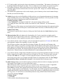
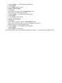
Swept-Field User Guide
Note: for more details see the Prairie user manual at http://www.prairietechnologies.com/resources/software/PrairieView.html
Please report any problems to Julie Last ([email protected]) or Brian Burkel ([email protected])
To turn on system
1.
2.
3.
4.
5.
6.
7.
8.
Turn on laser power supply
Turn key on laser power supply
1-3 are located behind and to left of scope
Turn shutter switch on
Carefully turn on camera – do not knock or jar
Turn on the computer (master switch on back of cart) and monitor
Turn on the microscope (switch on back right of microscope)
Start Prairie View software
Select objective either in the software in the Nikon controls window or on the LHS of the microscope.
The Prairie View software will automatically update the objective selection.
9. Loading the sample: To load the sample, tilt back the top of the microscope.
10. To look through eyepiece select eye on the front of the microscope. The light can be turned on and off
on the left side of the microscope.
11. For confocal imaging select L100 on the front of the microscope.
Dichroics
Dichroics can be changed by removing panel on Sweptfield scanner (left side of microscope). The
dichroics are held in place with a magnetized holder
Additional dichroics for laser can be found in a small black case
Prairie View
Note: Some sections have extra controls accessible through a green bar located to the left of the section.
SFC Settings
 Choosing imaging settings:
Slit or pinhole imaging can be used – choose your aperture
Slit mode = faster, but lower resolution
Pinhole mode = slower, but better resolution
 Choose appropriate emission filter
o
o
o
o


FITC/TRITC
460/50
535/50
605/70
Galvo mode: use linear. Do not use sinusoidal mode with this camera
Synchro method: Bulb mode vs timed mode
 Bulb mode and Timed mode refer to the synchronization between the camera and
the scanner. For this camera the recommendation is to use Bulb
Camera settings
 Gain (3e-, 6e-, 12e-): This is the number of electrons needed per intensity unit. 12e- is the most signal
per unit but the lowest sensitivity
 EM Gain: Use this to adjust the contrast in the image. It is an exponential function between 0 and 4095.
It will typically be set ≥3700.
 Read out mode: Leave at 5MHz (M)
 Exposure time: can increase to get more signal
 Binning: This determines the spatial resolution. 2x binning takes 2x2 pixels and counts them as one
pixel. This increases the signal per pixel but decreases the resolution.
Image Window Size (upper left of windows)
 Image Window Size controls the way in which the image is displayed in the window.
 “Fit” will change the image to fit within the window.
 1:1 will show the image at its actual size as defined by Image Size.
 Smaller will decrease image by 10% (click repeatedly to continue decreasing size).
 Larger will increase image by 10% (click repeatedly to continue increasing size).
Photoactivation time per pixel
 Controls photoactivation time
Scanning panel is located on the top right hand corner of the main control window.
 Scanning controls image acquisition.
 Live scan will continually scan the object and update the image.
 Single scan will scan the object once and display that image.
 New window will open a new imaging window.
 Running frame average is used with live scanning.
 If the box is checked for running frame average, the software will average the number of
frames indicated in the box.
 Averaging frames can increase signal to noise ratio and resolve an image.
 Averaging frames is only useful if the object is not being moved.
 Average every N frames is used with single scan.
 This function will average the number of frames indicated in the box.
 A higher number will result in a higher signal to noise ratio.
 Objective Lens is important to set. (This has not been done yet for the SFC)
 Select the objective lens being used. This is important for scale bars.
Stage Control is located under the Scanning panel.
 Before beginning to move the Stage Controls, it is useful to hit both 0s in the panel to bring all settings
to “home.”
 The right set of arrows can be used to set the top and bottom positions of a z-stack.

Step sizes (um) can be changed by entering a number in the appropriate box.
The tabs halfway down the main control window contain additional controls and experimental setups.
The Laser tab controls the power given to the laser.
 Specify channels for each laser
 Turn on laser power
The Z-Series tab controls the settings for creating z-stacks.
 The top and bottom positions as well as step size can be set here or in the Stage Control panel above.
 The number of slices wanted can be set in this tab.
 Four values are needed to set z-series parameters – start position, stop position, step size, and number of
slices. When any three values are set, the fourth will be automatically calculated.
 If “Adjust PMT & Laser” is checked, different power and gain settings can be entered in the data table.
Can use a power gradient to define laser powers.
 A Z-series can be saved so that the same series can be used again.
 Save Path is used to save the data to a particular location on the computer.
The T-Series tab controls the settings for creating a series of images and data using various parameters
regions of interest and Z-series.
 A cycle can be set up by changing values in the data table.
 A new cycle can be added or inserted in the Add/Insert Cycle panel by clicking “Single Image.”
 Waits can be inserted into the series by clicking “Wait.”
 Iterations indicates the number of times the cycle will repeat.
 Z-series can be added using the drop down menu in the data table.
 To start running the T-series you have created, click “Start T-Series.”
 Save Path is used to save the data.


T-Series Preferences (under preferences menu)
T-Series Execution Order: Determines whether to do all iterations at a given XY stage location before
proceeding to the next XY stage location – (1) T-Series Iterations - (2) XY Stage Locations - (3)
Cycles – or to perform each iteration at all XY stage locations before proceeding to the next iteration –
(1) XY Stage Location - (2) T-Series Iterations - (3) Cycles.
TriggerSync Execution: TriggerSync experiments can be executed two different ways, either the
software will wait for the entire experiment to finish before the next cycle starts, or the next cycle can be
started directly after the TriggerSync experiment is started – Start next cycle immediately
The Misc tab contains the main Save Path for saving your data. The photoactivation mask can also be
selected in the misc tab.
The Image Window also contains important controls and settings.
 To the left of the pictures are the channel buttons. Ch1/Ch2/Ch3/Ch4 indicates which channel is being
shown in that image window. The small rectangle directly to the right of the channel buttons allow you
to choose the color that that particular channel is shown in.
 Can click bar to right of channel button to select range check. This is used to check for image saturation
and can be controlled by changing the gains.
 “Freeze” will freeze the current image in the window. Data will continue to be collected, but it will not
be shown in the frozen window.
 BOT (brightness over time) can be used to watch the change in pixel intensity over time.



LUT (look up table) can be used to observe the intensity of acquired data. The intensity of an image can
be changed without affecting the raw data. This is a useful way to test whether you can use less power.
ROI (region of interest) can be used to choose an area of the image to zoom into. Unlike optical
zooming, region of interest selection does not create a power issue. Image size is chosen automatically
when using ROI.
The button with a graph image can be used to display a plot of intensity values in each channel along a
line that you create on the image.
The Labels tab gives the user the flexibility to define and save a set of operational parameters for imaging
control including laser power, PMT settings, channels and pixel dwell time. It is also possible to set up
label groups for more complicated or multi-laser applications.
Creating and Using a Label
1. Press Add Label. A row named “Label-001” with current settings will be created.
2. To change the name of the label, double-click on the box with “Label-001” in it and rename as
desired.
3. To change any of the settings associated with the label, first adjust the setting in the appropriate place
(for example, an increase in laser power would be done in the Laser tab). It is then necessary to select
Update Label Values.
4. Selection of a specific label is done by clicking on a label listed under the Label Select drop-down
menu.
The Photoactivation (PA) tool enhances the functionality of a Z-series acquisition or single scans by
allowing the user to apply masks to scan areas, controlling where laser power is applied. These masks
can be on specific z-slices, applied to an entire stack or a single scan.

To use the PA tool for a stack of images, a Z-series must first be acquired, see Z-Series tab. While still
in the playback window after acquiring a Z-series, select PA.
This will open a toolbar on the right side of the Image Window. By using the scroll buttons at the
bottom of the window or cursor keys to change frames and the buttons on the right to edit the masks, the
mask region(s) are defined. These are the regions that are scanned by the laser beam. Regions that are
not masked are not scanned. The selected regions are shown as translucent green areas on the image as
shown below. When all masks are defined, disable the PA mask editing mode (Click PA).

To use the PA tool for a single image click PA at any time except when in playback mode for a Z-series.
Define a single slice PA mask as you would a set of masks for a Z-series. To use the mask it must be
selected on the Misc tab. To acquire a Z-series using these masks, it will be necessary to set up a Tseries, being sure to select a set of masks in the PA column. It is important to make sure Save images
generated when Photo Activation (PA) is used? is also checked in the Preferences menu.
The Mark Uncage dialog is used to mark locations of points for photo activation or uncaging experiments.
These points can be single or in a user-defined line or grid.
Note: Although the Mark Uncage function can be performed in a PrairieView window, TriggerSync
must be open and running (from the Applications menu) in order to use this function.
When Mark is selected, a box appears on the image in the active Image Window and a second, Mark
Uncage, window appears (as shown below). To select points, click on the appropriate option in the Mark
window and follow the steps described below. Because this window is an interface between PrairieView
and TriggerSync, it is necessary to set the Mark parameters using a Mark Points Wizard, which is
accessed by clicking Configure.
To Mark a Point:
1. Click Point.
2. Move point to desired location on image.
3. Click Configure... to set Mark Points parameters.
4. Click Prepare.
5. Click Acquire to mark points.
To Mark a Line of Points:
1. Click Line.
2. Enter number of points in the X Point Density field.
3. Move line to desired location on image.
4. Click Configure... to set Mark Points parameters.
5. Click Prepare.
6. Click Acquire to mark points.
To Mark a Grid of Points:
1. Click Grid.
2. Enter number of points in X and Y Point Density fields.
3. Move grid to desired location on image by dragging center point.
4. Resize and rotate grid by dragging corners.
5. Click Configure... to set Mark Points parameters.
6. Click Prepare.
7. Click Acquire to mark points.
Note: If the PA does not occur at the marked points let us know – it may need a new calibration file.