Download LS 13 320 Laser Diffraction Particle Size Analyzer

Standard Operating Procedure for:
LS 13 320 Laser Diffraction Particle Size Analyzer Operation
(Particle Sizer R01.doc)
Missouri State University
and
Ozarks Environmental and Water
Resources Institute (OEWRI)
Prepared by: __________________________________
OEWRI Quality Assurance Coordinator
Date: _____________
Approved by: __________________________________
OEWRI Director
Date: _____________
ID: PS
Revision: 1
March 2008
Page 2 of 38
Table of Contents
1
Identification of the method ......................................................................................... 3
2
Applicable matrix or matrices...................................................................................... 3
3
Detection Limit ............................................................................................................. 3
4
Scope of the method .................................................................................................... 3
5
Summary of method ..................................................................................................... 3
6
Definitions ..................................................................................................................... 4
7
Interferences ................................................................................................................. 8
8
Health and safety .......................................................................................................... 8
9
Personnel qualifications .............................................................................................. 8
10
Equipment and supplies .............................................................................................. 8
11
Reagents and standards .............................................................................................. 9
12
Quality control .............................................................................................................. 9
13
Calibration and standardization .................................................................................11
14
Procedure ....................................................................................................................13
15
Data acquisition, calculations, and reporting............................................................24
16
Computer hardware and software ..............................................................................29
17
Method performance ...................................................................................................29
18
Pollution prevention ....................................................................................................30
19
Data assessment and acceptable criteria for quality control measures..................30
20
Corrective actions for out-of-control or unacceptable data .....................................30
21
Waste management .....................................................................................................31
22
References ...................................................................................................................31
23
Tables, diagrams and flowcharts ...............................................................................31
24
Contacts for Instrument Support
ID: PS
Revision: 1
March 2008
Page 3 of 38
1
Identification of the method
Operation of the LS 13 320 Laser Diffraction Particle Size Analyzer.
2
Applicable matrix or matrices
This instrument can be used for natural sediment samples.
3
Detection Limit
The aqueous liquid module (ALM) is capable of suspending samples in the size
range of 0.04 µm to 2000 µm. The Polarization Intensity Differential Scattering (PIDS)
assembly provides the primary size information for particles in the 0.04 µm to 0.4 µm
range. The PIDS assembly also enhances the resolution of the particle size distributions
up to 0.8 µm. This additional measurement is necessary as it is very difficult to
distinguish particles of different sizes by diffraction patterns alone when the particles are
smaller than 0.4 µm in diameter. Repeatability is 1% about mean size.
4
Scope of the method
This standard operating procedure provides Missouri State University (MSU)
Ozarks Environmental and Water Resources Institute (OEWRI) laboratory personnel
procedures for the operation of the LS 13 320 Laser Diffraction Particle Size Analyzer.
5
Summary of method
Sediment samples are collected and stored in ambient conditions in Temple Hall.
Information about the sample (i.e., collection time, temperature, preservative, etc.) is
recorded on the sample bag and sample collection form. Sediment samples are
disaggregated, sieved to < 2 mm size, and transferred to sample tubes. Samples are
pretreated with hydrogen peroxide and acetic acid to remove organic matter. The
addition of sodium-hexametaphosphate enhances separation and dispersion of
aggregates before sonification. The samples are loaded into the auto-prep station (APS)
after pretreatment.
The APS sonicates each sample and adds the sample to the ALM bath by
flushing the sample tube with water. The ALM contains filtered tap water that suspends
the sample and the ALM sonicates the sample and uses a circulating pump to disperse
the sample in the tap water. Water used for this analysis is pumped from a holding tank
that contains heaters which keep the water at a constant temperature. The sample is recirculated in a closed-loop system while it is delivered to the sample cell in the optical
bench.
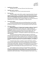
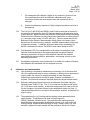
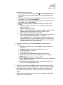
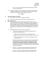
The optical system (Figure 1) consists of a source of illumination, a sample
chamber where the sample interacts with the illuminating beam, a Fourier lens system
that focuses the scattered light, and an array of 126 photodetectors that record the
scattered light intensity patterns. Diffraction scattering patterns from 0.4 µm to 2000 µm
are measured by 119 of the126 photodetectors. The remaining seven detectors are
associated with the PIDS assembly and measure particle size in the 0.4 µm to 0.4 µm
range.
When a sample reaches the sample cell, the sample load is measured and
diluted until a standard obscuration percentage is attained. Then the detector array
records the composite diffraction scattering pattern of the sample. The size distribution is
computed by straightening the set of numbers for each size classification which are
represented by each channel detector. The relative amplitude of each number is used
ID: PS
Revision: 1
March 2008
Page 4 of 38
as a measure of the relative volume of equivalent spherical particles of that size class.
The straightening of the data set is based on the Fraunhofer or Mie theories of light
scattering from particles.
Figure 1. LS 13320 optical system
It is difficult to distinguish particles of different sizes by diffraction patterns alone
when the particles are smaller than 0.4 µm in diameter. Therefore particles in the 0.04
µm to 0.4 µm range are measured by the PIDs assembly that utilizes the remaining 7 of
126 photodetectors in the array. The PIDS assembly illuminates the particles
sequentially with vertically and horizontally polarized light from three different visible
wavelengths and the differential scattering patterns produced are measured 36 times.
One photodetector is dedicated to measuring the intensity of the un-scattered light to
determine the amount of obscuration. The PIDS measurements are added to the same
straightening matrix that is used for determining size distribution using laser diffraction
patterns alone to integrate the two measurements methods and produce one data set.
6
Definitions
6.1 Alignment Measurement: LS 13 320 pre-run cycle procedure that monitors the
alignment of the laser beam to ensure that it is automatically aligned within 1-2
microns of the center of the detector array on the horizontal and vertical axes.
This procedure obtains the light intensity patterns (diffraction or PIDS) from which
the size distribution is calculated and ensures instrument accuracy.
6.2
Analytical batch: A set of samples processed at the same time.
6.3
Aqueous Liquid Module (ALM): The Aqueous Liquid Module presents the entire
sample to the sample cell in the optical bench by re-circulating the sample through
hoses. The system is controlled using software commands. The ALM system
consists of: the sample vessel containing the suspension fluid and dispersed
ID: PS
Revision: 1
March 2008
Page 5 of 38
sample particles; the sample cell; the sonicator that aids in the dispersion of the
sample during the run cycle; the variable speed circulation pump that circulates the
particles through the sample cell; the inlet and drain hoses; the hoses to transfer
fluid from the vessel to the sample cell; and liquid level sensors.
6.4
Auto Prep Station (APS): The Auto Prep Station is used in conjunction with the LS
13 320 optical bench and the Aqueous Liquid Module (ALM). It is capable of
adding dispersant as well as sonicating a total of thirty aqueous samples. The
APS transfers the entire amount of each individual sample to the ALM vessel by
rinsing the sample tube with water for a preset, OEWRI-selected time.
6.5
Background: The background flux pattern provides information about the
cleanliness and integrity of the tap water used for sample dilution. The background
flux intensity limits are as follows:
a. The flux counts within Channels 1 and 2 must be <4.0 x 106.
b. The flux counts for the sum of Channels 10 through 40 must be <2.0 x 106.
c. The Channel between 95 and 126 that has the highest flux counts cannot
exceed 30.
6.6
Bench sheet: The sample tracking sheet used in the laboratory that links sample
identification and sample procedures performed. The bench sheet for these
procedures is located in Appendix A.
6.7
Calibration verification standard (CVS): A standard consisting of a known sample
media used to calibrate the instrument during initial setup, monitor the instruments
recognition of initial calibration, and to quantify batch accuracy. Results of CVS
analyses are reported as % differential volume. CVS used for this procedure are
provided by the instrument manufacturer (Beckman Coulter) and consist of two
size fractions: 15 µm garnet (G15) and 500 µm glass beads (GB500).
6.8
d10, d50, d90: Particle size distribution is reported as the grain diameter at 10%
(fine tail), 50% (median), and 90% (course tail) of a cumulative percent frequency
distribution curve where each point illustrates the percentage of the total sample
weight accounting for the weight of all grains smaller than a certain diameter (d).
This allows the description of wide ranging data sets, since particle diameters can
span many orders of magnitude for natural sediments. The LS 13 320 actually
accounts for the area of the cumulative curve and not the weight because the
instrument dilutes the sample to decrease interference during scattering.
6.9
Detector channel: Various optical paths, or focus areas, of a detector array
associated with laser diffraction. Each channel consists of a light sensitive detector
surface and associated amplifying electronics.
6.10 Field duplicate (FD): Two samples taken at the same time and place under
identical circumstances which are treated identically throughout field and laboratory
procedures. Analysis of field duplicates indicates the precision associated with
sample collection, preservation, and storage, as well as with laboratory
ID: PS
Revision: 1
March 2008
Page 6 of 38
procedures.
6.11 Laboratory duplicate (LD): An aliquot of the same environmental sample treated
identically throughout a laboratory analytical procedure. Analysis of laboratory
duplicates indicates precision associated with laboratory procedures but not with
sample collection, preservation, or storage procedures.
6.12 Laser diffraction: Technology that correlates laser beam diffraction patterns to
particle size. Particles are suspended in water, diluted, and passed through a cell
where a laser beam is directed. Particles scatter the beam and a series of
photodetectors placed at different angles measures the diffraction pattern caused
by the scattering. Smaller particles scatter the laser beam at larger angles than
bigger particles. Light scattering theory is used to derive the sizes of particles in
the sample and particles are assumed to be spherical. Samples are diluted to omit
interference by re-scattering.
6.13 Measure Loading: A LS 13 320 function that measures the amount of light scatter
from the presence of particles from each sample, calculates loading rates,
determines the prescribed obscuration percent as specified in the Standard
Operating Method (SOM), and dilutes the sample until the specified obscuration
percentage is obtained. Sample dilution deletes interference between particles
within the sample which sharpens the light intensity pattern and provides an
acceptable signal-to-noise level in the detector channels.
6.14 Minimum Quantification Interval: The lowest level that can be quantified accurately
and is generally defined as four times the method detection limit = 4(MDL).
6.15 Natural standard (NS): A sample of a known particle size distribution and that has
composition similar to environmental samples being analyzed. The NS undergoes
the same preparatory and determinative procedures as the environmental samples
and is used to evaluate accuracy along with the calibration verification sample
(CVS). ES63 and ES250 are used for OEWRI projects. Both originate from an
engineering sand sieved to produce a size range of 63µm < x < 125µm and 250µm
< x < 500µm respectively.
6.16 Obscuration: The amount of light scatter from the presence of particles within a
laser beam. Run cycle options within the Standard Operating Method (SOM) have
been preset to produce desired obscuration values for laser diffraction alone or
with the use of polarization intensity differential scattering (PIDS) analysis. Project
management and laboratory personnel should discuss the anticipated fractions of
the environmental samples prior to analysis to determine if the additional PIDS
enhancement is desired which will dictate the obscuration setting.
a. Appropriate obscuration values for analyses using laser diffraction
alone are 8% to 12%.
b. When PIDS sizing is used in addition to laser diffraction, the
obscuration should be set to Standard Obscuration in the
ID: PS
Revision: 1
March 2008
Page 7 of 38
corresponding SOM. This setting will allow sample analysis when
PIDS values range from 40 to 60%.
6.17 Offsets: Bias voltages from the amplifier circuit of the instrument that may cause
electrical noise in a detector channel. These bias voltages from the amplifier circuit
are measured before every run cycle in order to “zero out” or establish an electrical
noise baseline at the detector channel. The signal at each detector channel does
not go to zero in the absence of light, so the measured bias voltage intensity is
subtracted from the diffraction pattern from the sample to improve sizing accuracy.
6.18 Polarization Intensity Differential Scattering (PIDS): An assembly that provides the
primary size information for particles in the 0.04 µm to 0.4 µm range and enhances
the resolution of the particle size distributions up to 0.8 µm. This is an additional
measurement that differentiates particles smaller than 0.4 µm in diameter that are
indistinguishable using laser diffraction patterns alone.
6.19 Preference file (.prf): A program that includes options relating to data presentation
and output formats. The preference file used in this procedure is:
OEWRI_Standard_Preferences.prf. This preference file exports grain size
distribution data for each sample as differential volume % for each of the 126
channel listings. Statistical data consisting of mean, mode, d10, d50, and d90 is
exported for each sample with the preference file as well. Project specific reference
files can be created or edited to fit project specific needs as determined by the
project manager and laboratory director.
6.20 Relative Percent Difference (RPD): A measure of method precision calculated as
the difference between a sample and duplicate results, divided by the average of
the sample and duplicate results, multiplied by 100%.
Relative percent difference (RPD):
(A-B)
AVERAGE(A,B) 100
A = original sample concentration
B = duplicate sample concentration
6.21 Standard Operating Method (SOM): Programs that control the instrument settings
and automatic sampler to ensure consistent analyses and improve precision. The
SOM that is used for natural sediment samples is titled
OEWRI_Standard_SOM.som and includes preset sample analysis protocol
pertaining to run cycle options, Auto Prep Station sample handling, and run
settings. Project specific SOMs can be created or edited to fit project specific
needs as determined by the project manager and laboratory director.
6.22 Standard Operating Procedure (SOP): Protocol that consists of instrument and
Auto Prep Station settings as well as data presentation and data output formats.
The SOP is divided into two distinct components; a SOM (Standard Operating
Method) (.som) file and a Preference (.prf) file.
ID: PS
Revision: 1
March 2008
Page 8 of 38
7
Interferences
External mechanical vibration, if present, may cause misalignment of the laser.
Automatic alignment occurs before every analysis as preset into the SOM. Electrical
interferences can occur, but are unlikely because the instrument is connected to an
uninterruptible power supply. Sudden changes in temperature can cause misalignment
as well as changes to the measured electrical offsets. Users will record the time and
temperature at the instrument before analysis. Optimal temperature range is 10 to 35°C
and relative humidity range is 0 to 85%. The optical bench is completed enclosed so that
background laboratory light does interfere with scatter patterns. The Fourier lens
focuses on the incident beam so it will not interfere with the scattered light. The
instrument is calibrated by the manufacturer and certified installer.
8
Health and safety
The LS 13 320 contains a 5 mW diode laser. This Class 3a laser does not
produce a hazard if viewed for only momentary periods with the unaided eye, but may
present a hazard if viewed using collecting optics. The instrument therefore may pose
certain hazards associated with low-power lasers if misused. All maintenance
procedures associated with the laser will be performed by the laboratory supervisor only.
Never look directly into the laser light source or at scattered laser light from any
reflective surface. To comply with Federal Regulations (21CFR Subchapter J) as
administered by the Food and Drug Administration's (FDA) Center for Devices and
Radiological Health (CDRH), defeatable microswitches are located on the right and left
of the door panel. Do not tamper with or attempt to defeat the safety interlock switches.
A copy of ANSI standard 2136.1, SAFE USE OF LASERS, is located near the
instrument for reference.
Review the MSDS for information and safety concerns regarding the standard
powders or dispersants used throughout these procedures. Specifically note that a 30%
hydrogen peroxide (H2O2) solution is used during sample pretreatment and should not
come in contact with the skin because it is a strong oxidizing agent.
9
Personnel qualifications
Samples will be analyzed by Missouri State University (MSU) Ozarks
Environmental and Water Resources Institute (OEWRI) laboratory personnel who have
received appropriate training from experienced personnel, prior coursework, and
laboratory experience regarding the analyses, and who are familiar with all of OEWRI’s
sample handling and labeling procedures and appropriate SOPs.
10
Equipment and supplies
10.1
Beakers: 10ml and 250ml
10.2
Carousel: part of Auto Prep Station assembly; loads samples into the instrument,
30 sample capacity.
10.3
Centrifuge: International Clinical Centrifuge, 1.2 amp, serial # AC1428.
ID: PS
Revision: 1
March 2008
Page 9 of 38
10.4
Chain of Custody Forms: used to describe the written record of the collection,
possession and handling of samples. Chain of custody (COC) forms are located
on a board in Temple Hall 125. Chain of custody forms should be completed as
described in the Chain of Custody SOP # 1030R01.
10.5
Daigger Vortex Genie 2: Tube votex, cat no. G22220.
10.6
Flasks: 500ml and 1000ml
10.7
Labeled sample tubes: 13ml
10.8
Micro-spatulas: used to transfer sample or standards into sample tubes.
10.9
Protective Gloves: for protection against chemicals and from contaminants.
10.10 Sonicator: Omni Ruptor 400.
11
12
Reagents and standards
11.1 G15: Coulter LS Control G15 (ref 7800370) 15µm garnet.
11.2
GB500: Coulter LS Control GB500 (ref 7800372) 500µm glass beads.
11.3
ES63: Engineering sand sieved to produce a size range of 63µm < x < 125µm.
11.4
ES250: Engineering sand sieved to produce a size range of 250µm < x <
500µm.
11.5
1% Acetic acid: Pour 400mL of de-ionized (DI) water into a clean 500-mL
volumetric flask. Transfer approximately 5ml of acetic acid into a clean beaker
and use a pipette to transfer 5 ml of acetic acid to the flask containing DI water.
Dilute to 500ml with DI water. Danger: Corrosive.
11.6
30% Hydrogen peroxide (H2O2): Pre-made solution that can be purchased from
Fisher Scientific, H325-500. Caution: Strong Oxidizer.
11.7
3% Sodium hexametaphosphate (NaPO3n) Dispersant Solution: Weigh 30g of
sodium hexametaphosphate in a weighing tray and transfer it to a 1-L volumetric
flask. Pour 500ml of de-ionized water into the flask and swirl to dissolve. Dilute
to volume with addition DI water. NaPO3n can be purchased from ELE
International, 24-4145 (CAS: 10124-56-8).
Quality control
12.1 Quality control program: The minimum requirements of the quality control
program for this analysis consist of an initial demonstration of laboratory
capability and the analysis of background and standard check samples as a
ID: PS
Revision: 1
March 2008
Page 10 of 38
continuing check on performance. The laboratory must maintain performance
records that define the quality of the data that are generated.
12.2
Initial Accuracy and MDL Determination – See Appendix B to review procedures
used to determine initial accuracy, precision, and MDL for these analyses.
12.3
Initial Operator Precision and Accuracy – To establish the ability to generate
precise and accurate results, the operator shall perform 5 replicates of the grain
size standards G15, ES63, and ES250. The mean (x), standard deviation (s),
and coefficient of variation (CV%) of each particle size category will be calculated
for each standard analyzed. The mean values of each particle size category
should be within ±10% of the mean values associated with the initial accuracy
and precision determination listed in Appendix B to be considered accurate. The
CV% of each of the 5 analyses should be within ±20% to be considered precise.
12.4
A background measurement provides information about the cleanliness and
integrity of the water used for sample dilution and eliminates any interfering
signal due to possible light leakage or scattering from dust on lenses or any
particulate matter present in the optical path by comparing the current
background levels to the background levels set for the instrument during set-up
and calibration.
a.
Tap water, used to dilute each sample, is the only matrix measured for
the background determination.
b.
Tap water is warmed to approximately 50°F within a holding tank and
pumped to the ALM to provide consistency that is not normally found from
using water from the tap alone. Degassing associated with temperature
changes from incoming tap water caused bubbles to form in the sample
matrix. These bubbles were not dissociated from particles in the sample,
but measured as particles within the sample which decreased accuracy and
precision. A holding tank and heaters were added to the system to
eliminate the false positives within detector channels. See Appendix C for
holding tank information.
c.
Background is measured between each sample analysis as dictated by
the SOM.
d.
The background measurement serves as a laboratory reagent blank.
e.
Background flux pattern data is recorded between each sample analysis
and is delivered to the QA/QC Coordinator with each project data set. The
QA/QC Coordinator randomly chooses a background flux pattern from each
carousel, performs calculations, and compares data to the established
limits. Background standards are reported as achieved or not achieved
with each data report. If background limits are not achieved, the carousel is
re-analyzed.
ID: PS
Revision: 1
March 2008
Page 11 of 38
13
f.
If the background flux pattern is higher in any channel by a factor of two,
the contaminant source will be identified, maintenance will occur,
corrections will be made, and samples from that carousel will be reanalyzed.
g.
Contact the laboratory supervisor if faulty background patterns continue to
be observed.
12.5
The CVS (G15), NS (ES63 and ES250), and LD will be analyzed at the start of
the analytical cycle and after every 52 sediment samples or at least twice during
a batch analysis. Batch accuracy and precision will be determined by calculating
Relative Percent Difference for each particle size classification or value reported
(i.e., phi sizes, mean, mode, d10, d50, d90, etc.). The true values listed on the
Beckman Coulter Particle Characterization Assay Sheet or the mean values
derived from the initial accuracy, precision, and MDL determination will be used
to determine accuracy. In addition, all channel data will be reviewed by the
QA/QC coordinator for outliers. The RPD for each value should be ±20%.
12.6
Field Duplicate (FD): Two samples taken at the same time and place under
identical circumstances which are treated identically throughout field and
laboratory procedures. Analysis of field duplicates indicates the precision
associated with sample collection, preservation, and storage, as well as with
laboratory procedures.
12.7
All calibration and quality control information is recorded in the batch information
and calibration file associated with the analyses and user.
Calibration and standardization
13.1 Light scattering is an absolute measurement technology only in the sense that
once the experimental setup is correct, calibration or scaling are not necessary in
order to obtain the volume (or weight) percentage of each component.
Calibration is determined by the optical design, therefore no calibration is
required. The instrument measures electrical offsets and aligns the laser beam.
13.2
Reference background files are saved in the calibration files folder using the
filename format: ZLBYYYY.$ls. The YYYY are the last four digits of the optical
LS 13 320 bench serial number. A reference background file is used to monitor
the any changes in the diluent (filtered, room temperature water) over time. A
reference background file is not used in this procedure, however, a reference file
may be set-up.
13.3
The preferences file (.prf) includes options relating to data presentation and
output formats. The preference file used in this procedure is:
OEWRI_Standard_Preferences.prf. This preference file exports grain size
distribution data for each sample as differential volume % for each of the 126
channel listings. Statistical data consisting of mean, median, mode, d10, d50,
and d90 is exported for each sample with the preference file as well. Project
ID: PS
Revision: 1
March 2008
Page 12 of 38
specific reference files can be created or edited to fit project specific needs as
determined by the project manager and laboratory director.
13.4
The Standard Operating Method (SOM) is a program that controls the
instrument settings and automatic sampler to ensure consistent analyses and
improve precision. The SOM that is used for natural sediment samples is titled
OEWRI_Standard_SOM.som and includes preset sample analysis protocol
pertaining to run cycle options, Auto Prep Station sample handling, and run
settings. Standard templates for SOMs are in the SOP folder and are used by
selecting Run and loading the appropriate SOM. The OEWRI Standard SOM
measures the LD range from 0.37519µm to 2000µm and does not include PIDS
data. Project specific SOMs can be created or edited to fit project specific needs
as determined by the project manager and laboratory director. NEVER MODIFY
SOMs. Individual templates with specific SOMs for various media and
preferences for data display can be made before analyses and saved specifically
for a project. The laboratory manager is the only person authorized to make
changes to the SOMs, so these activities need to occur before the day of
analyses, plan accordingly. The following settings are used for
OEWRI_Standard_SOM.som:
Run Cycle Options: Offsets, alignment, and background measurements will be
measured between each sample.
Auto Prep Station sample handling:
 Sample tube is sonicated for 30 seconds on the highest setting (8)
 Fluid is added for 2 seconds during sonication
 Sample tube is flushed and emptied for 3 seconds
 Sample is loaded into the ALM circulation bath and diluted until Standard
Obscuration settings are attained.
ALM and Run Cycle Settings:
 Pump speed: This is currently set to 60%. Pump speed should be changed
to optimize the project specific samples. You should select a pump speed
that is sufficient to suspend the largest diameter particle.
 Run length for particle measurement is 60 seconds and does not include
PIDS data.
 Optical model: Default is Fraunhofer.rf780d. After samples are analyzed,
other optical models like Mie Scattering may be selected and the data recomputed. See the reference list for more information on studies testing
different optical models (e.g., Eshel et al., 2004).
13.5
The aqueous liquid module (ALM) is capable of suspending samples in the size
range of 0.04 µm to 2000 µm. The Polarization Intensity Differential Scattering
(PIDS) assembly provides the primary size information for particles in the 0.04
mm to 0.4 mm range.
13.6
The instrument will be maintained as defined in the user manual or as QA/QC
data dictate.
ID: PS
Revision: 1
March 2008
Page 13 of 38
14
Procedure
14.1 Initial sample preparation procedures for natural sediment samples consist of:
a. Dry each sample in oven at 60ºC. This may take 7 days or more depending
on conditions during sample collection.
b. Disaggregate each dry sample with mortar and pestle.
c. Sieve each sample through a 2mm sieve.
14.2
Determine whether PIDS data is required for the project. If data from the ultra
fine range is desired, sediment samples with require additional sieving and the
SOM will have to be edited to include PIDS. If PIDS data is not required,
continue with the procedures written in this SOP.
Optimal Sample Mass Determination
14.3 Use the following to determine a sample mass that satisfies the “Standard
Obscuration” values as recommended by the LS 13 320 software. The
appropriate sample mass will minimize the number of dilutions necessary to
obtain the correct obscuration values for all channels optimizing the Auto Prep
Station. Dilutions provide an acceptable signal-to-noise level in the detector
channels, because if too many particles are present, light already scattering from
one particle would likely be scattered from another which blurs the light intensity
pattern. Representative samples will be chosen from the project, weighed using
various masses, manually loaded into the ALM (Aqueous Liquid Module), and
analyzed. The Measure Loading function, that measures the amount of light
scattered out of the beam when particles are introduced into the sample cell, will
be used to measure and observe each obscuration value associated with each
sample mass. The optimal sample mass for the project will be derived from the
obscuration values observed. Follow the procedures below to determine the
optimal sample mass for the project.
a. Chose samples that represent typical project characteristics. The project
manager and laboratory QA/QC coordinator should be consulted.
b. The project manager and laboratory QA/QC coordinator should be consulted
to establish the “start mass” and “finish mass” to increase the speed of this
determination because optimal sample mass can vary from 100mg to 400mg.
Pre-determined masses of each sample will be in 50mg increments to speed
processing. Generally, the finer the sample, the less amount of sample that
will be required, so samples with more silt or clay will require less sample
mass.
c. Place a weighing paper on the balance, tare the balance, and weigh sample.
Transfer sample into a bar coded test tube. Continue weighing samples
according to predetermined masses and weigh a corresponding duplicate for
each predetermined sample mass. For example, if the start mass is 100mg
and the finish mass is 200mg, there will be two 100mg, two 150mg, and two
200mg aliquots of each representative sample. Transfer each sample into a
ID: PS
Revision: 1
March 2008
Page 14 of 38
bar-coded test tube and record the sample ID and corresponding sample
tube bar code on the bench sheet located in Appendix A.
d. Use the flask with calibrated automatic dispenser labeled “3%
Hexameta.soln.” to add 3ml of de-ionized (DI) water to each sample in the
tubes. Put on gloves and goggles. Use a pipette to deliver 600µl of 30%
H2O2 to each sample. Use a different pipette to add a 1 drop of 1% acetic
acid solution to each sample tube. Monitor the samples after adding the
H2O2, as some samples may foam aggressively. If samples foam
excessively, overwhelming the sample tube, add a small amount of DI water
to the sample to dilute the reaction.
e. Set the Daigger Vortex Genie to the Touch setting and set the speed at 4-5.
Separately place each tube on the platform and stir each sample for at about
5 seconds.
f.
Place the sample tubes back in the tube rack and let the samples digest for
24 hours.
g. Set the centrifuge to power 5, insert samples into a centrifuge, and centrifuge
each sample for approximately 3 minutes. Decant the clear supernatant
liquid using the vacuum pump and attached flask, while retaining all of the
sediment in the tube.
h. Repeat procedures 13.3d through 13.3g.
i.
Observe the sediment. A completely digested sediment sample should be
significantly lighter in color than the undigested sediment. Exceptionally
organic rich sediments that are very dark brown in color and generally
containing > 10% organic matter may require additional digestion treatment.
In addition, the sample may require an additional digestion treatment if it
effervesces excessively when shaken. Contact the project manager
regarding additional treatment procedures.
j.
Use the flask with calibrated automatic dispenser labeled “3%
Hexameta.soln.” to add 3 ml of 3% sodium-hexametaphosphate to each
sample and stir sample using the Vortex Genie for at about 5 seconds. Place
the sample tubes back in the tube rack and allow the samples to soak for
approximately 5 minutes.
k. Sonicate each sample with the independent sonicator (Omni Sonic Ruptor
400) for 1 minute to disperse the sample. To operate the sonifier: turn the
power switch to the on position (located on the back of the panel); place the
sample tube under the sonicator tip, immerse the tip in the sample; press the
Start button and slowly increase the power to 30 (as read on the power
output display on the top of the panel). Place the samples tubes back in the
tube rack and cover the samples with the bench sheet associated with the
samples until they can be manually analyzed.
ID: PS
Revision: 1
March 2008
Page 15 of 38
l.
Manually analyze each sample.
1. Turn on optical module by selecting Run Use Optical Module. Allow
optical bench to warm up approximately 15 minutes before beginning
analyses.
2. Check the ALM bath to ensure that dilution water is at the second liquid
level sensor. If not, select Control  Fill.
3. To analyze samples using the Run Cycle option versus a SOM, click on
Run Cycle, and then New Sample.
4. Make the following changes to the default settings in the Run Cycle
window:
i.
Deselect the first Auto Rinse box, then select Auto Rinse at the
bottom of the list.
ii.
Deselect “include PIDS data”.
iii.
Make sure the following boxes are checked: Measure offsets, Align,
Measure background, Measure Loading, and Start 1 Run.
iv.
Select “Sonicate during loading” at Power 2.
v.
Select Options and make sure that the “By Standard Obscuration” is
selected under Sample loading Options. Click OK.
vi.
Select Sample Info. Fill in the appropriate File Name, Sample ID,
and any comments to be saved with the sample. View the filename
template in lower left corner to make ensure that the correct sample
info was entered. Click OK when finished.
m. In the Run Cycle window, select Run Settings and make necessary
changes:
i. Set the pump speed to 60. Increase speed if grains remain in the
ALM bath.
ii. Set Run Length for 60 seconds (the default run time).
iii. Sonicate during run at Power 2.
iv. The number of runs is 1.
v. Check boxes for Compute Sizes during run and Save File.
vi. Nothing should be selected under “Before first run” or “Between
Runs.”
vii. Select Model and click on Fraunhofer.rf780d.
viii. Select Folder and change the folder directory where the sample data
will be saved if necessary.
viiii.Click OK when completing all of these steps within the Run Cycle
window and proofing changes made.
n. In the Run Cycle window, click Start to initiate the instrument to measure
offsets, auto align, and measure background. Observe background results.
If the background flux pattern is higher in any channel by a factor of two,
identify the contaminant source, make corrections, and re-analyze the
sample.
o. When the screen reads “Obscuration 0%: Low, Add Sample” add the first
sample mass to the ALM bath.
ID: PS
Revision: 1
March 2008
Page 16 of 38
p. Monitor the laser diffraction obscuration values at the top of the Measure
Loading window.
If the screen reads “Obscuration XX%: Low, Add Sample”, the
obscuration is unacceptable and the sample concentration is too low,
skip to step “q.” to flush the system and allow the analysis of a larger
pre-measured mass from the set.
ii. If obscuration is “High”, dilution is necessary, select Control  Dilute
Once. Allow the sample obscuration values to stabilize and monitor
the new obscuration values. If the values are still not acceptable,
dilute once again. Keep track of how many times the sample is
diluted. Do not dilute more than 3 times, skip to step “q.” to flush the
system and allow the analysis of a smaller pre-measured mass from
the set.
iii. If obscuration is “OK” the initial obscuration is acceptable as is the
sample mass associated with the analysis. Note this mass and
continue to step “q.”
i.
q. Select Start Analysis which is located in the lower left corner of the screen.
This will measure the sample regardless of obscuration and flush the system
to allow the analysis of the next pre-measured mass from the set.
r.
Continue to analyze each sample mass by repeating step “p” or until the
optimal sample mass is determined.
s. Operators will inform the QA/QC coordinator upon completion of the sample
mass analyses.
QA/QC Preparation
14.4 The CVS (G15), NS (ES63 and ES250), and LD will be analyzed at the start of
the analytical cycle and after every 52 sediment samples or at least twice during
a batch analysis. Each carousel holds a maximum of 30 samples. The CVS
(G15), NS (ES63 and ES250), and LD will occupy the first four slots of the first
project carousel and will occupy slots 26-30 of the second carousel. Choose a
laboratory duplicate randomly per carousel from samples being analyzed from
that carousel. Use Table 2 to prepare the CVS, NS, and LD.
Table 1. QA/QC Preparation
Source
G15
Mass (mg)
150
ES63
ES250
2500
6000
LD
Optimal
mass
determined
in Section
13.3
ID: PS
Revision: 1
March 2008
Page 17 of 38
Place a weighing paper on the balance, tare the balance, and weigh each
standard or laboratory duplicate. Transfer each mass into a bar-coded test tube
and record the sample ID and corresponding sample tube bar code in a project
data book. The CVS’s (G15) and NS (ES63 and ES250) do not require any
pretreatment. Load these tubes into the appropriate slots in the carousel.
Sample Preparation
14.5 After determining the optimal sample mass in Section 13.3, take each sample
through the following procedures.
a. Place a weighing paper on the balance, tare the balance, and weigh sample.
Transfer each sample into a bar-coded test tube and record the sample ID
and corresponding sample tube bar code on a bench sheet.
b. Use a flask with a calibrated automatic dispenser and labeled “DI Water” to
add 3ml of de-ionized (DI) water to each sample in the tubes. Put on gloves
and goggles. Use a pipette to deliver 600µl of 30% H2O2 to each sample.
Use a different pipette to add a 1 drop of 1% acetic acid solution to each
sample tube. Monitor the samples after adding the H2O2, as some samples
may foam aggressively. If samples foam excessively, overwhelming the
sample tube, add a small amount of DI water to the sample to dilute the
reaction.
c. Set the Daigger Vortex Genie to the Touch setting and set the speed at 4-5.
Separately place each tube on the platform and stir each sample for at about
5 seconds.
d. Place the sample tubes back in the tube rack and let the samples digest for
24 hours.
e. Set the centrifuge to power 5, insert samples into a centrifuge, and centrifuge
each sample for approximately 3 minutes. Decant the clear supernatant
liquid into a 250ml beaker while retaining all of the sediment in the tube.
g. Observe the sediment. A completely digested sediment sample should be
significantly lighter in color than the undigested sediment. Exceptionally
organic rich sediments that are very dark brown in color and generally contain
> 10% organic matter may require additional digestion treatment. In addition,
the sample may require an additional digestion treatment if it effervesces
excessively when shaken. Contact the project manager regarding additional
treatment procedures.
h. Use the flask with calibrated automatic dispenser and labeled “3%
Hexameta.soln.” to add 3 ml of 3% sodium-hexametaphosphate to each
sample and stir sample using the Vortex Genie for at about 5 seconds. Place
the sample tubes back in the tube rack and allow the samples to settle for
approximately 5 minutes.
ID: PS
Revision: 1
March 2008
Page 18 of 38
i.
Sonicate each sample with the independent sonicator (Omni Sonic Ruptor
400) for 1 minute to disperse the sample. To operate the sonifier: turn the
power switch to the on position (located on the back of the panel); place the
sample tube under the sonicator tip, immerse the tip in the sample; press the
Start button and slowly increase the power to 30 as read on the power output
display on the top of the panel. Place the samples tubes back in the tube
rack and cover the samples with the bench sheet associated with the
samples until they can be manually analyzed.
Pre-analysis Procedures
14.6 Access the software and load the carousel following the procedures below.
a. Turn on the power strip located on the wall above the pump. The pump and
water heaters are plugged into this power strip. See Appendix C for water
tank information. Observe the water temperature. It is recommended that
water temperature be 20°C (68°F) or above for sample analyses. Record the
dilution water temperature in the project notebook.
a. Record ambient laboratory conditions such as temperature and humidity in
the project notebook.
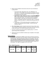
b. Turn on computer and log on with user name and password.
c. Click LS 13320 desktop icon. Click OK to acknowledge the copyright and log
on with user name and password to access the software.
Figure 2. LS 13320 logon screen.
d. Click Run  Use Optical Module.
ID: PS
Revision: 1
March 2008
Page 19 of 38
Figure 3. LS 13320 Optical Module screen.
e. Click Control  Pump On to turn the ALM pump on. Make sure that the
ALM bath is free of debris and water is to the fill line. Rinse the bath to
remove particles by selecting Control  Rinse and allow the bath to rinse
until it appears clean. Click Cancel on the ALM rinse window to turn the
rinse cycle off. The bath will automatically fill to the correct water level when
the rinse is turned off.
f.
Advance the Auto Prep Station (APS) carousel to the home position, by
selecting Control  Carousel to Home. The carousel will automatically
advance Slot 1 to the home position which is just before the APS sonicating
device.
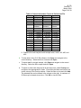
g. Load sample tubes into carousel slots, according to the table below :
ID: PS
Revision: 1
March 2008
Page 20 of 38
Table 2. Sample Loading Order
Sample Type
G15 Standard
ES63 Standard
ES250 Standard
Lab Duplicate
Natural Sediments
Carousel #1
Carousel Slot No.
1
2
3
4
5-30
SOM File Used
G15_Garnet_SOM_alm_ap
E63_Sand_SOM_alm_ap
ES250_SOM_alm_ap
OEWRI_Standard_SOM
Carousel #2
Sample Type
Natural Sediments
G15 Standard
ES63 Standard
ES250 Standard
Lab Duplicates
Carousel Slot No.
1-26
27
28
29
30
SOM File Used
OEWRI_Standard_SOM
G15_Garnet_SOM_alm_ap
E63_Sand_SOM_alm_ap
ES250_SOM_alm_ap
OEWRI_Standard_SOM
h. If the project requires additional carousels, odd numbered carousels should
mirror the sample loading order of Carousel #1 and even numbered
carousels should mirror the sample loading order of Carousel #2. All project
analyses should end with the analysis of each standard and a laboratory
duplicate from a sample within the carousel.
i.
Tip each tube toward the center of the carousel to facilitate carousel
movement.
j.
Continue with procedures in Section 14.7 after the instrument has been
powered on for at least 15-minutes.
Sample Analysis
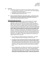
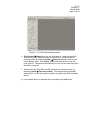
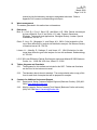
14.7 Select Run Run Auto-Prep Station from the toolbar. A window entitled “Run
the Auto-Prep Station – By slot number” like the one below should be visible.
ID: PS
Revision: 1
March 2008
Page 21 of 38
Figure 4. “Run the Auto-Prep Station – By slot number” screen.
14.8
Activate Slot 1 that contains the G15 Lab Standard by clicking the box next to the
slot number. Type the File ID, Sample ID, and any necessary comments into the
row that corresponds with the carousel slot chosen. Choose the appropriate
SOM from the drop down list in the column labeled “SOM or SOP”. Appropriate
SOMs are listed in Table 3 above.
14.9
Activate Slot 2 that contains the ES63 Natural Standard by clicking the box next
to the slot number. Type the File ID and Sample ID information into the column
that corresponds with the carousel slot chosen. Add any additional information to
the Comments box. Choose the appropriate SOM from the drop down list in the
column labeled “SOM or SOP”. Appropriate SOMs are listed in Table 3 above.
14.10
Activate Slot 3 that contains the ES250 Natural Standard by clicking the box
next to the slot number. Type the File ID and Sample ID information into the
column that corresponds with the carousel slot chosen. Add any additional
information to the Comments box. Choose the appropriate SOM from the drop
down list in the column labeled “SOM or SOP”. Appropriate SOMs are listed in
Table 3 above.
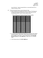
14.11 Continue to activate each of slots 4 through 30 (or the appropriate ending slot
number) by clicking the box next to the slot number and typing the File ID’s and
sediment sample IDs. Choose the appropriate SOM from the drop down list in
the column labeled “SOM or SOP”. Appropriate SOMs are listed in Table 3
above.
14.12 Review all information in the “Run the Auto-Prep Station – By slot number”
window to ensure that all sample IDs correspond to the correct tube and slot
number.
ID: PS
Revision: 1
March 2008
Page 22 of 38
14.13 Click Start to begin analysis. The instrument will measure offsets, align the laser
and detector, and measure background. The screens will look similar to those
below.
Figure 5. Measuring offsets screen.
Figure 6. Auto align screen.
ID: PS
Revision: 1
March 2008
Page 23 of 38
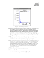
Figure 7. Normal background screen.
14.14 Observe the background intensity flux patterns test box. The graph should mirror
the one above. Contact the laboratory supervisor if excessively high or low
background patterns are observed. Background flux patterns for each carousel
should be reviewed before many additional samples are analyzed to decrease
the number of samples that may have to be re-analyzed due to unacceptable
variations in the background flux patterns. To check the graph of the background
flux pattern on a sample run click View, then Intensity, then Graph followed by
Background (Flux).
14.15 The operator can leave the instrument after all samples are loaded and
background measurements are determined to be within limits, however, the
instrument should be monitored periodically during sample analysis.
14.16 As sample measurements are completed, the carousel may be filled and slots reselected while the remaining samples are analyzed. As the sample analysis is
completed, the sample slot information becomes gray. To refill the slot with
additional samples, reactivate the Slot number by checking the box next to the
slot number and filling in the appropriate information. Be sure and insert the
correct sample tube for the sample information entered and change SOM
information if necessary.
14.17 Refer to Section 15.1 for data retrieval procedures.
14.18 Instrument Shut Down
a. At the end of the analyses click Control Pump off.
ID: PS
Revision: 1
March 2008
Page 24 of 38
b. Flip the switch to off on the power strip located on the wall above the pump to
turn off the holding tank water pump and water heaters.
c. Turn the optical module off by exiting the software.
d. Log off and turn the computer off.
14.19 Area Clean Up
a. Use a damp sponge to wipe the carousel and area around the ALM clean.
b. Remove sample tubes from the ALM bin and wipe out the bin.
c. Rinse used sample tubes with DI water and place them upside down in a rack
to dry.
d. Close the ball valve between the water filter and copper water line by moving
the lever to the closed position.
e. Remove sample bags and other personal items from the area.
15
Data acquisition, calculations, and reporting
15.1 Follow the procedures below to acquire particle size data. Data is stored as
“.$ls” files that the LS 13 320 software uses for data presentation.
a. Load the preference file: OEWRI_Standard_Preferences.prf. This Preference
file exports the following data for each sample:
i.
Sample information in the formats illustrated below: analysis time and
date, file name, file ID, Sample ID, operator, bar code, and comments.
Table 3. Sample Information Format of Preferences File
LS
9:41 8 Nov 2007
Dig Test_2Dig-H2_2007-11-07_13File name:
19_01.$ls
File ID:
Dig Test
Sample ID:
2Dig-H2
Operator:
Gwenda J. Schlomer
Bar code:
Comment 1:
Comment 2:
ii. Channel list with corresponding differential % volume detected with
particle analysis in that channel:
ID: PS
Revision: 1
March 2008
Page 25 of 38
Table 4. Channel Information Format of Preferences File
Dig Test
Dig Test
Dig Test
Channel _2Dig-H2
_2Dig-L1
_2Dig-L2
Diameter _2007-11
_2007-11 _2007-11
(Center) -07_16-45
-07_16-02 -07_16-10
um
_07.$ls
_02.$ls
_03.$ls
Diff.
Diff.
Diff.
Volume
Volume
Volume
0.393
1.22E-06
0.002138
0.00209
0.432
1.98E-05
0.00263
0.002587
0.474
0.000127
0.003904
0.003872
0.520
0.000456
0.007353
0.007348
0.571
0.000961
0.01553
0.015503
0.627
0.001736
0.030317
0.030094
…
…
…
…
1314
0
0
0
1443
0
0
0
1584
0
0
0
1739
0
0
0
1909
0
0
0
iii. Statistics for each sample include sample mean, mode, d10, d50, and
d90.
b. To view data in the LS 13 320 software, click Open and navigate to the
correct directory. Select the file to view and click Open.
c. To export data for a single sample, click Open and navigate to the correct
directory. Select the file to export and click Open.
d. To export or view more than one file at the same time, select Overlay and
navigate to the appropriate file folder. Files within the folder are listed in the
center column of the Overlay window. Select the files to view and click Add.
The selected files can be viewed in the column on the right. A maximum of
20 files may be viewed at one time. Click OK to view the files.
ID: PS
Revision: 1
March 2008
Page 26 of 38
Figure 8. Overlay screen.
e. To export multiple files at one time as an Excel (.xls) file select Overlay and
navigate to the appropriate file folder. Files within the folder are listed in the
center column of the Overlay window. Select the files to view and click Add.
The selected files can be viewed in the column on the right. A maximum of
20 files may be viewed at one time. Make sure that the options illustrated
below are checked in the overlay window. Click OK to view the files. Click
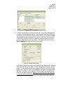
RunFile  Export to open the Export Data window.
Figure 9. Export Data screen.
In the Export Data window, select the following boxes: Sample Info, Statistics,
Size Listing, and Export All Runs. Choose the appropriate directory and file
option. To use a directory other than the default directory, select the middle
option under “Export To”, then select Folder and navigate to the appropriate
file folder. Click OK. In the “Export As” text box, type in an appropriate file
name for the exported data file. Make sure to leave the Excel file extension
(.xls) at the end of the file name. Click Export. Repeat the overlay and
export procedures until all the samples for the project have been exported
ID: PS
Revision: 1
March 2008
Page 27 of 38
into an Excel file. Copy the exported folder to a removable flash drive for
further processing in Excel.
15.2
Follow the procedures below to export background data.
a. Load the preference file: Background_Intensity_Listing.prf. This Preference
file exports the background intensity flux count for each channel and the
corresponding detector number for each sample selected:
Table 5. Background Intensity Listing of Preferences File
Detector
Number
…
BDWetlands BDWetlands BDWetlands
_BD1AO_
_BD1BI_
_BD1BO_
_2008-03
_2008-03
_2008-03
-18_13-30
-18_13-38
-18_13-46
_0...
_0...
_0...
Background Background Background
0
38400
31560.5
31416.4
0.5
45114.9
38926.7
39501.1
1
631259
616961
623469
2
1.34E+06
1.27E+06
1.26E+06
3
510794
492858
488354
4
370289
341680
331661
…
…
…
124
10.5355
10.1875
10.5624
125
9.99587
9.68284
10.0814
126
9.6515
9.36997
9.77349
127
0
0
0
b. To view and export the background intensity flux for associated with samples
previously exported, select Overlay, add the appropriate files to the file list,
and click OK (to view the files). In the Overlay window, select Graph 
Background (flux), then View  Listing. Channels 0 to 127 should be
listed.
c. In the Overlay window, click RunFile  Export.
ID: PS
Revision: 1
March 2008
Page 28 of 38
Figure 10. Export Background Data screen.
In the Export Data window, select the following boxes: Sample Info,
Intensity Listing, and Export All Runs as illustrated above. Choose the
appropriate directory and file option. To use a directory other than the
default directory, select the middle option under “Export To”, then select
Folder and navigate to the appropriate file folder. Click OK. In the
“Export As” text box, type in an appropriate file name for the exported
data file. Make sure to leave the Excel file extension (.xls) at the end of
the file name. Click Export. Repeat the overlay and export procedures
until all the samples for the project have been exported into an Excel file.
Copy the exported folder to a removable flash drive for further processing
in Excel.
15.3
Reporting results: Results should be reported to 0.01 %.
15.4
Relative percent difference (RPD):
(A-B)
AVERAGE(A,B) 100
A = original sample concentration
B = duplicate sample concentration
15.5
Standard Deviation: The evaluation of MDL and precision require calculation of
standard deviation. Standard deviations should be calculated as in equation 2.
∑ x2 – [ (∑ x)2/n)]
s = { --------------------------- } ½
n-1
Where:
n = number of samples,
x = concentration in each sample.
ID: PS
Revision: 1
March 2008
Page 29 of 38
Note: This is the sample standard deviation calculated by the STDEV
function in Microsoft Excel.
15.6
Coefficient of Variation (Cv%): Accuracy can be calculated by determining the
coefficient of variation which is the standard deviation of the multiple sample
measurements divided by the mean of those measurements.
Cv% = (s/ x )100
16
Computer hardware and software
16.1 Microsoft Word: this document is prepared using Word.
16.2
17
The Word document file name for this SOP is: Partical Sizer R01.doc
Method performance
17.1 Method performance data for SOMs are available through the LS 13 320
software. The aqueous liquid module (ALM) is capable of suspending samples in
the size range of 0.04 µm to 2000 µm. The Polarization Intensity Differential
Scattering (PIDS) assembly provides the primary size information for particles in
the 0.04 mm to 0.4 mm range. The PIDS assembly also enhances the resolution
of the particle size distributions up to 0.8 mm. Repeatability is 1% about mean
size.
17.2
The desired performance criteria for these analyses are:
a.
There are three background flux intensity limits established by the
manufacturer and are listed below:
i. The flux counts within Channels 1 and 2 must be <4.0 x 106.
ii. The flux counts for the sum of Channels 10 through 40 must be <2.0 x
106.
iii. The Channel between 95 and 126 that has the highest flux counts
cannot exceed 30.
Background flux pattern data is recorded between each sample analysis
and is delivered to the QA/QC Coordinator with each project data set.
The QA/QC Coordinator randomly chooses a background flux pattern
from each carousel, performs calculations, and compares data to the
established limits. Background standards are reported as achieved or not
achieved with each data report. If background limits are not achieved, the
carousel is re-analyzed.
b.
Precision: ± 20%, precision data will be reported as relative percent
difference and project managers will determine what data is used.
c.
Accuracy: ± 20%, accuracy data will be reported as relative percent
difference and project managers will determine what data is used.
ID: PS
Revision: 1
March 2008
Page 30 of 38
d.
Minimum Quantification Interval: 0.01%.
18
Pollution prevention
All wastes from these procedures shall be collected and disposed of according to
existing waste policies within the MSU College of Natural and Applied Sciences.
Volumes of reagents made should mirror the number of samples being analyzed. These
adjustments should be made to reduce waste.
19
Data assessment and acceptable criteria for quality control measures
19.1 The analyst should review all data for correctness.
19.2
Relative percent difference (RPD) will be calculated for pairs of duplicate
analyses to determine precision. Two laboratory duplicates (LD) will be randomly
selected from each set of 52 samples and analyzed. Precision data will be
reported as relative percent difference and project managers will determine what
data is used. The desired precision is ± 20%.
19.3
The CVS (G15) and NS (ES63 and ES250) will be analyzed at the start of the
analytical cycle and after every 52 sediment samples or at least twice during a
batch analysis. Accuracy will be determined by calculating Relative Percent
Difference for the true values listed on the Beckman Coulter Particle
Characterization Assay Sheet. All channels will be reviewed by the QA/QC
coordinator for accuracy. The RPD should be ±20%.
19.4
The background flux intensity limits are as follows:
a. The flux counts within Channels 1 and 2 must be <4.0 x 106.
b. The flux counts for the sum of Channels 10 through 40 must be <2.0 x 106.
c. The Channel between 95 and 126 that has the highest flux counts cannot
exceed 30.
20
19.5
The background flux pattern cannot vary in any channel by a factor of 2 or
higher.
19.6
The completed Excel spreadsheet is reviewed by the analyst’s supervisor or the
OEWRI QA officer.
Corrective actions for out-of-control or unacceptable data
1201 If data are unacceptable for any reason, the analyst should review their analytical
technique prior to conducting this analysis again.
20.2
The results for background, precision, and accuracy are compared to acceptable
values for this analysis. If any results fail to meet criteria, the samples
associated with the failed criteria will be reanalyzed.
20.3
The instrument may require trouble shooting techniques if the data are
unacceptable. All instrument maintenance will be performed as outlined in
ID: PS
Revision: 1
March 2008
Page 31 of 38
manual and by the laboratory manager or designated technician. Refer to
Appendix D for common troubleshooting techniques.
21
Waste management
The wastes generated in this method are not hazardous.
22
References
Blott, S.J., Croft, D.J., Pye, K., Saye, S.E., and Wilson, H.E., 2004. Particle size analysis
by laser diffraction. Pye, K. and Crofts, J.D. (eds). Forensic Geoscience:
Principles, Techniques, and Applications. Geological Society, London, Special
Publications, 232: 63-73.
Eshel, G., Levy, G.J., Mingelgrin, U., and Singer, M.J., 2004. Critical evaluation of the
use of laser diffraction for particle-size distribution analysis. Soil Science Society
of America Journal, 68: 736-734.
Loizeau, J.L., Arbouille, D., Santiago, S., and Vernet, J.P., 1994. Evaluation of a wide
range laser diffraction grain size analyzer for use with sediments. Sedimentology
41: 353-361.
LS 13 320 Laser Diffraction Particle Size Analyzer Instrument Manual © 2003 Beckman
Coulter, Inc., 11800 SW 147th Ave., Miami, FL 33196
23
Tables, diagrams and flowcharts
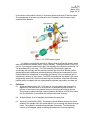
23.1 The diagrams for this method are included in this SOP. Tables and flowcharts
can be found in the instrument manual.
23.2
24
The laboratory bench sheet is attached. The analyst should make a copy of this
form for each rack of samples that will be prepared for analysis.
Contacts for Additional Instrument Support
24.1 Dana Leech, Senior Customer Support Engineer (Beckman Coulter): (305) 6065694, [email protected]
24.2
Mervin Yaremko, Senior Customer Tech Support (Beckman Coulter call center):
(800) 742-7694 [email protected]
APPENDIX A - Bench Sheet
Project:
Date:
Lab
Personnel:
BATCH #
Samples Included
Digestion 1
Digestion 2
Disp./Son.
QA/QC Samples:
Pretreatment
Checklist
ID: PS
Revision: 1
March 2008
Page 33 of 38
APPENDIX B – Initial Accuracy and MDL Determination
Two Calibration Verification Standards (CVS) and two Natural Standard (NS) were analyzed 10
times and results were used to determine initial accuracy and the Method Detection Limit (MDL) in the
targeted size ranges associated with the standard. CVS used for this procedure are provided by the
instrument manufacturer (Beckman Coulter) and consist of two size fractions: 15 µm garnet (G15) and
500 µm glass beads (GB500). The NS has a known particle size distribution and has composition
similar to environmental samples being analyzed. OEWRI projects use the ES63 and ES250 which is
an engineering sand sieved to produce a size range of 63µm < x < 125µm and 250µm < x < 500µm.
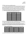
Data from each channel was combined to produce the following size categories based on Phi
sizes commonly used to characterize class limits (National Research Council):
Table 6. Size Categories (National Research Council)
Size Category
Size Category
Size Range (µm)
Name
Abbreviation
Very Coarse Sand
VCS
2000 -1000
Coarse Sand
CS
1000 - 500
Medium Sand
MS
500 - 250
Fine Sand
FS
250 - 125
Very Fine Sand
VFS
125 - 62.5
Course Silt
CSi
62.5 - 31.3
Medium Silt
MSi
31.3 - 15.6
Fine Silt
FSi
15.6 - 7.8
Very Fine Silt
VFSi
7.8 - 3.9
Clay
Clay
3.9 - 0.4
Very Fine Clay
<0.4
The CVS G15 provides accuracy data for the MSi and FSi size categories. The NS ES63 provides
accuracy data for the FS and VFS size categories. The NS ES250 provides accuracy data for the MS
size category. The CVS GB500 provides accuracy data for the CS size category.
Accuracy of these initial analyses was determined by calculating the Relative Percent Difference
(RPD) using data from the Beckman-Coulter Control Assay Sheets associated with the CVS and
previous accuracy analyses of the NS. Beckman-Coulter only provides the mean value of the data set
on the assay sheet for the G15 standard and only provides the d10, d50, and d90 of the data set for the
GB500 standard. The acceptable RPD is ±10% and all standards passed QA/QC for accuracy.
Table 7. Accuracy Determination
Standard
True Values
G15
ES63
Mean = 15.14
FS = 55.37
VFS = 42.35
d10 = 502
d50 = 563
d90 = 632
GB500
MDL Analysis
Values (n=10)
Mean = 14.29
FS = 50.89
VFS = 45.98
d10 = 505.1
d50 = 568.7
d90 = 639.9
RPD
5.81
8.43
-8.21
0.62
1.01
1.24
Precision of these initial analyses was determined by calculating the Coefficient of Variation
(CV%) between size category data from each of the 10 analyses for each of the standards. The
ID: PS
Revision: 1
March 2008
Page 34 of 38
acceptable RPD is ±10% and all standards passed QA/QC for precision relative to the target size
categories.
Table 8. Precision Determination
Standard
G15
ES63
ES250
GB500
Size Category
MSi
FSi
FS
VFS
MS
CS
CV%
0.82
0.57
6.05
5.68
2.10
0.42
The initial accuracy determination established standard size category mean values for each
standard within the target size category and those means are listed below. The NS ES250 was
analyzed 10 times to provide accuracy data for the MS size category and will be used for regular
accuracy determinations due to cost associated with the GB500 laboratory standard.
Table 9. Mean Values for Regular Accuracy Determinations
Standard
Size Category
G15
MSi
FSi
FS
VFS
MS
CS
ES63
ES250
GB500
Mean Value
(Differential Volume Percent)
43.03
36.26
50.89
45.98
66.22
95.85
These mean values will be used to compare data from each analysis of each standard and determine
accuracy of each batch of samples as described within this SOP.
The typical procedures used to determine the method detection limit are not applicable for
analyses using the LS 13 320. Measure loading and offset functions used for LS 13 320 analyses do
not allow the measurement of a laboratory blank. Prescribed obscuration percentages are specified in
the Standard Operating Method (SOM) and samples are diluted until the specified obscuration
percentage is obtained to provide an acceptable signal-to-noise level in the detector channels. Blanks
are not recognized in the software and obscuration values set for sample analysis cannot be obtained if
no sample is present during measurement. Therefore background flux patterns are used in place of
actually analyzing a laboratory blank. The background flux pattern provides information about the
cleanliness and integrity of the tap water used for sample dilution. There are three background flux
intensity limits established by the manufacturer and are listed below:
a. The flux counts within Channels 1 and 2 must be <4.0 x 106.
b. The flux counts for the sum of Channels 10 through 40 must be <2.0 x 106.
c. The Channel between 95 and 126 that has the highest flux counts cannot
exceed 30.
Background flux pattern data is recorded between each sample analysis and is delivered to the
QA/QC Coordinator with each project data set. The QA/QC Coordinator randomly chooses a
background flux pattern from each carousel, performs calculations, and compares data to the
ID: PS
Revision: 1
March 2008
Page 35 of 38
established limits. Background standards are reported as achieved or not achieved with each data
report. If background limits are not achieved, the carousel is re-analyzed.
ID: PS
Revision: 1
March 2008
Page 36 of 38
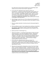
APPENDIX C - Water Tank Assembly for Beckman Coulter LS 13 320
Photo 1. Water Tank Assembly for Beckman Coulter LS 13 320.
PARTS:
1. Water Tank: 35-gallon, Roto Mold
2. Water Filter Cartridges: CUNO Ultra Block Filter Model GRUBB5N- 5µm rating (Grainger
product #5PT91)
Water Filter Housing: USOM-38-S Point-of-Use Water Filter (from Grainger)
Water Pump: Iwaki Magnetic Drive Pump Model MD-70RLZT
Float Valve: Nylon Space-Saving Float Valve (www.mcmaster-carr.com)
Heaters: 2- 200Watt Submersible Aquarium Heaters
Ball Valves: ¾ inch (NPT), between tank and pump; ½ inch (NPT), between pump and
instrument and between instrument and tank.
8. Bleeder Valves: ½ inch size.
3.
4.
5.
6.
7.
ID: PS
Revision: 1
March 2008
Page 37 of 38
APPENDIX D
Troubleshooting
1. “Backgrounds too negative in 1 channels. (99)”: Sample material may be collecting in the
instrument causing high diluent background values (i.e., the background flux patterns measured
during the Measure Background function detected residual material in the water prior to the sample
being loaded). This problem usually occurs if the pump speed is too low or sample size is too large.
Adjust sample size and/or pump speeds as appropriate if this problem occurs frequently. A
thorough cleaning of the instrument will generally remediate the problem. To clean the instrument:
Mix up 10% cleaning solution (Micro Cleaner): add 10ml of cleaner to 1-liter
volumetric flask; dilute to volume.
Select Control  Rinse; allow instrument to rinse for at least 5 minutes.
Select Control  Open Drain; fill the instrument (in the ALM) with the cleaning
solution.
Allow the cleaning solution to circulate in the instrument for at least 1-hour.
Drain the instrument and rinse for about 5-min, or until the diluent appears clean
(suds-free).
2. Loud beeping noise (liquid level sensor), sometimes accompanied by an error message,
“The vessel is too full, please drain some fluid.”: The overflow liquid level sensors in the ALM
bath detect fluid on the sensor therefore the instrument alerts the user that the vessel is
overflowing. Check the sensors for water droplets and wipe them clean. The beeping should stop.
3. Unable to drain instrument (after selecting Control  Open Drain): Sample material,
especially if running a large quantity of fine material, tends to accumulate around a brass ball
located at the 90° turn of the inlet hose in the lower right corner of the ALM. To fix this problem,
remove the cover of the ALM, and find the metal plate that houses the brass ball (see photo below).
Carefully detach the metal plate with an allen wrench (size 5/64 in or 2mm) then using tweezers, lift
the metal ball and quickly check to make sure there is no residue on the ball. Be careful not to lift
the ball out of place for very long as the water in the line is under pressure and removing the ball
will cause water to flow from the line into the ALM. Most of the time, the ball just needs to be briefly
lifted or adjusted instead of cleaned.
ID: PS
Revision: 1
March 2008
Page 38 of 38
Remove these
bolts using an
allen wrench (5/64
in). Reattach as
arrows indicate.
Photo 2. Inside the ALM: illustrates a portion of the ALM bath and the 90° turn of the inlet hose
in the lower right corner of the ALM.