Download user`s manual to get an idea of it`s

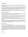
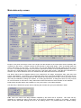
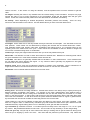
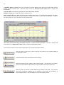
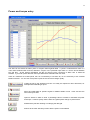
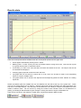
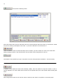
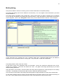
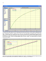
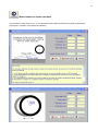
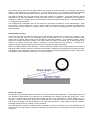
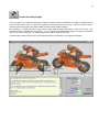
1
Software User’s Manual
Version 1
Tony Foale Designs © 2007
Last revision 24/11/2007
2
Introduction
Estimation of acceleration and top speed performance is often considered a simple matter. Multiply engine
torque by the gear ratios and add aerodynamic drag and weight into the calculation mix and “hey presto” you
have all the answers.
Reality is of course somewhat different. There are many more factors to take into account if you want to get as
accurate a picture as possible. For example; CG height affects load transfer to the driven wheel as well as
determining the tendency toward terminal wheelies. The height of the frontal aerodynamic centre of pressure
also has a similar influence. Load transfer affects tyre slip which in turn affects the relationship between RPM
and road speed, which in turn determines the power available at any particular road speed. Then there is the
influence of the dead time between gear changes when no power is being transmitted.
This software takes all those factors, and more, into account and raises the bar of performance estimation to a
new level for enthusiasts and racers of all levels. It is an invaluable tool to help with the proper evaluation of
gearing strategies and gear change points.
What will the software do?
Simply put, it will produce calculated estimates of the straight performance of a motorcycle. However, there is
really a lot more to it than that and there are a lot of contributing factors to ultimate performance. When fed with
the appropriate data this software uses most of these factors in the calculations.
The user can enter the power / torque curves of the engine. This information is much more readily available
these days than it used to be and many people interested in performance will have there machines dyno tested.
Gear ratios, weight, drag, tyre properties, wheelbase and CG height are the other main factors which affect
performance and the software accepts values for these parameters. Although of lessor importance, the values for
wheel and crankshaft inertia can also be entered when known to further refine the results.
Outside of the motorcycle, performance is also affected by wind and the slope of the road surface, both of these
values can be included. The web sites of many race tracks have data regarding road elevation which can be
downloaded.
After the calculations have been made there are several graphical and tabular options for analysing the results,
and comparing different cases. These comparisons can be used to optimise some of the contributing factors
such as gear ratios, when to change gear, whether the CG is too high or too low, what effect would engine
modifications have etc., etc. If required the results data can be exported for use in external software such as
eXcel or other spreadsheets and calculation software.
What it will not do.
It will not substitute for lack of accurate input data.
In racing, success or failure is often measured in hundredths or even thousands of seconds after many minutes or
hours of racing. Therefore the percentage difference involved is very, very small and calculations of performance
are never going to achieve the same degree of accuracy. There are so many possibilities for errors in input data
that are greater than the expected performances differences. For example, even if we had wind tunnel data for a
motorcycle and rider, it is almost impossible to expect the rider’s position to be exactly the same when actually
riding. Maybe his elbow sticks out a bit more from one lap to another. No software can fully account for these
variations. However, that is not always so important because we are usually more interested in the small
differences rather than absolute values. This software will give results close to reality with a reasonable margin of
error, but the differences between runs with different gearing or gear change RPM etc. should be much more
representative of practice.
Tony Foale.
November 2007
5
Initial screen
There are several speed buttons to access various areas of the software, as follows
This is probably the most used button on the initial screen and it opens the main data entry
screen.
Takes you to the screen for entering the power or torque curve of the engine. Also accessible
from the data entry screen.
This opens a screen to enter the elevation of sections of the road or track. Not needed for a
level horizontal surface. Also accessible from the data entry screen.
Enables the simultaneous plotting of up to 10 cases for comparison. Also accessible from the
results display page.
6
Opens a calculator for estimating the moments of inertia of the wheels and tyres. Using the
default values will give good results.
A calculator using an easy method to obtain CG height.
Gives access to this user manual as well as the tutorial videos
Sends an email to Tony Foale Designs. We welcome all comments about the software as
well as suggestions to expand or improve it. [email protected]
Connects to the Tony Foale Designs web site. www.tonyfoale.com
As explained in the section on first use this button opens the licence management window.
7
Main data entry screen
Except for the power and torque curves of the engine and the elevation of the road surface all the necessary data
is entered on this screen. Perhaps complex at first sight but in reality quite simple. Some of the data fields may
ask for data which you don’t have. In most cases if you use the default values the final results will not be in error
by much. For example most people will not know the “Moments of Inertia” of the crankshaft assembly, in practice
this has only a small influence in most cases and only in the lower gears anyway. Data like this is included in the
software only for those situations where it is available to add a little refinement to the calculations.
The factors which have the biggest influence over performance are weight, aerodynamic drag, gear ratios and
engine characteristics. Of these it is the aerodynamic drag which is the least available but if you know the top
speed of the motorcycle being analyzed then the software can help determine the drag. Power and torque curves
can easily be obtained by testing the machine on a rolling dynamometer, or failing that, there are many sources
for such information on the internet. Many aftermarket exhaust manufacturers have this data on their websites.
Road surface elevation data is also available, for many race tracks, on the official websites.
The data entry is divided into groups and the following will consider each group and data field in detail.
CdA This is the value of the drag coefficient multiplied by the frontal area in sq.metres. This value will vary
depending on whether the rider is laying down on the tank for acceleration or sitting up for braking. Therefore
there are two data fields, although the one for the braking value is only enabled when the “Include braking”
8
feature is active. In the section on using the software, it will be explained how to use the software to get this
value.
CP height Normally this value is only available from wind tunnel testing or CFD calculation. Except at very high
speeds this value is not of major importance for the acceleration phase and the default value will give good
results. As this also varies with rider position there are data fields for acceleration and braking
Air density Varies depending on ambient temperature, barometric pressure and humidity. There are many
sources for this information on the internet. Use the default value if you don’t have other data for this.
CG height These values are for the fully loaded motorcycle with rider and all liquids. Two data fields for the two
rider postures. These values can be determined by weighing the machine with one wheel raised onto a block.
This parameter affects load transfer under both acceleration and braking and so it is important when we are
operating near to the traction limit of the tyres. It also controls the acceleration at which a wheelie or stoppie will
occur which is another limiting factor on acceleration.
Load on tyre Simply the weight measured under each tyre of the fully loaded motorcycle.
Wheel MoI The Moment of Inertia of each wheel about its rotational axis. Methods for measuring these values
are given elsewhere but in most cases the default values will work OK.
Crank MoI This data is not generally available without calculation or direct measurement. Such measurements
are not difficult but require stripping the engine. In any case this value is generally only significant in first gear
and even then is of minor importance.
Reverse crank This is a tick box to indicate the direction of rotation of the crankshaft. Leave it unticked for an
engine which rotates in the same direction as the wheels and tick it for one that runs “backwards”.
Wheelbase is the horizontal distance between front and rear axles.
Rolling force Also known as rolling resistance. Another factor which is not always easy to specify and may be
different between acceleration and braking. For example if the power characteristics were obtained using a
rolling road dynamometer then the rolling force contribution from the rear will already be accounted for, to some
extent, in the torque figures. In which case it will be the front tyre drag plus bearing friction and brake drag which
will be the main contributor. On the other hand if the power values are obtained from an engine or gearbox driven
dynamometer then we need to consider the extra drag from the rear and the chain.
Under braking it is very hard to estimate a value and it will depend on many things, some rider controlled. If the
bike has a slipper clutch or electronically controlled fly-by-wire throttle the value will be quite different from that
obtained with heavy engine braking which in turn is affected by which gear the rider has selected.
Tyre maximum µ Coefficient of friction. For modern tyres this is likely to be in the range of 1.0 to 1.2 on a good
dry surface. May be different between front and rear. The front value is only necessary if we are using braking.
Peak rear tyre slip All tyres slip to some extent when driving or braking and we get the maximum driving force
when the tyre is slipping by about 10 to 20%. This varies with the particular tyre and surface. Slip affects the
9
relationship between road speed and RPM under acceleration, and so controls the power available at any road
speed. In the absence of proper tyre data it is suggested to leave the value at the default 15%. The slip value is
not so important when calculating braking and there is no provision for entering the front value.
Tyre radius The rolling radii of the tyres when loaded.
Maximum distance The calculations cease at this distance. If you tick the ¼ mile box then the maximum
distance is set to 402 metres and the starting velocity to zero to enable calculation of standing start performance.
Start velocity The performance calculations begin with this velocity. The software automatically selects which
gear is engaged at this speed. This may be the velocity at which the bike exits a turn and begins accelerating
down a straight.
Final velocity This is only enabled when the “include braking” tick box is ticked. It will normally be zero if you
are interested in coming to a complete stop within the maximum distance specified or more likely it will be the
corner entry speed for a turn at the end of the straight.
Include braking Tick this if you wish to include braking within the specified maximum distance. Use this when
you know the distance from one corner exit to the next corner entry point as well as the exit and entry speeds.
This will help optimise performance from one corner to another.
Head wind Performance is affected by wind and here we can enter wind data. Use positive values for a head
wind and negative values for a tail wind.
This group defines the transmission data etc. There are two options for data specification which are determined
by the following selection:
10
If Gearbox ratios is selected then you must enter the actual gearbox ratios plus the sprocket teeth and the
primary or clutch reduction ratio. After data entry click on the Calculate overall ratios button to produce the
overall ratios.
If Overall ratios is chosen then just enter the overall ratios where indicated.
RPM for change This is simply the RPM to change gear at.
Gear change time is the dead time during gear changing when there is no power being applied to the wheel.
This varies a lot between riders and also depends on whether some form of quick shifter is employed. Is likely to
be in the range of 0.1 to 0.3 seconds in a racing environment.
This section of the screen simply reproduces the power – torque curves for information. To enter or modify these
curves click on the Enter power curve button to access the appropriate window.
The remaining controls on this screen are the buttons on the right hand side as follows.
Click this when all data entry is done to pass to the screen for the graphical display of
the calculation results.
Converts between metric and imperial units of measure.
Allows the saving and later loading of the motorcycle data. The data in the “Conditions”
group is not saved because this refers to the test conditions and not the motorcycle.
Opens a screen for the entry of data related to the elevation of the road – track surface.
This data is sometimes available from the websites of race tracks. Not needed for a
level horizontal surface. Also accessible from the initial opening screen.
11
Power and torque entry
The data can be entered as either power or torques values against RPM. If “power” is selected then there is a
units choice between BHP and kW, likewise if “torque” is the preferred input there is a choice of units between
Nm and lbf.ft. All the internal calculations use Nm for torque but the conversion is taken care of inside the
software. If you enter power data then the torque data will be calculated and vice versa.
There is a maximum of 20 data points, but it is not necessary to use them all, nor is it necessary to use constant
RPM increments. You can use more points in parts of the curve that change quickly.
Copies the plot to the clipboard so that it can easily be copied into other documents, for
example when illustrating a report.
Saves and loads data for specific engines or different states of tune. Does not save the
other motorcycle data.
Opens a window in which to enter a percentage value to increase or decrease the power
and torque. Useful to quickly see the effect of a global power change on performance.
Refreshes the plot after entering or modifying the data grid.
Returns to the main data entry screen with the power curve selected.
12
Road elevation screen
Obviously not all roads nor tracks are flat and horizontal, and gradients affect performance. This screen allows
the entry of road elevation data. Even though all internal calculations are done in metres, the data grid accepts
units of metres or yards and feet. This makes data entry easier depending on the units of the track data.
Elevation maps are available on the web sites of some tracks, the data for the back straight of the Almeria track in
southern Spain, as shown above, came from such a site.
This data can be saved and loaded later, so a library of track profiles can be built up. After entering or loading
elevation data you can choose to use the data or ignore it in the performance calculations. If you exit this screen
by clicking the Cancel button then no elevation data will be used. In other words the calculations are done using
a horizontal road. If you click the Use gradients button then all calculations will use the elevation data until the
Cancel button is clicked or the software restarted. When “use gradients” is active the following notice appears
on the main data entry screen;
Notes on data:
The data entry allows considerable flexibility. The elevation values have an arbitrary reference and so can be
entered in terms of elevation above sea level as in the above example. Alternatively, a zero reference level can
be defined anywhere, say at the start of the run, in which case the above elevation values could be entered as:
0, 0, 8, 12, 20 instead of 546, 546, 554, 558, 566. The software only considers the relative values.
The distance data does not have to cover the whole length of a run. If the performance analysis continues
outside of the range of the specified data the software assumes that the surface is horizontal outside of the
elevation data range.
13
Results plots
There are some special features available when the mouse pointer passes over the graph area.
•
X-hairs appear automatically showing the X-Y values.
•
Marking points. To mark a point, just click and release without moving the mouse. This will mark a point
on a graph and show the X-Y parameter values.
•
Line drawing. To draw a line, click and hold at the start and release at the end. The slope of the line will
be calculated and displayed.
•
Changing graph pages will remove the marks and lines.
•
The graph data can be saved in numeric form to a file, which can be later be used in the multi-plotting
feature to compare multiple cases.
•
The graph window can be saved to the clipboard and subsequently pasted into other software for creating
reports etc.
Several pre-defined plots are available and can be selected from the tabs at the top of the graph area. These
plots can be viewed against time or distance. Although these plots provide interesting and useful information they
only refer to the latest analysis. The real power of the software is in the ability to compare small differences in the
results of different cases. We can do this by saving the results of each scenario which can be differences in
gearing, just looking at different RPM for gear changes or seeing the effects of engine modifications etc.
There are two functions in the software to enable quick comparisons between different cases:
and
14
This opens the following screen:
Above the buttons there are two data boxes with the time and velocity data for the last run, above that is a data
entry box for entering a description of this case. If you want to add this run to the list click on:
There are buttons to save an retrieve this table, which is useful if you want to add to it or refer to it at a later date.
Without saving this table, it only remains active until you either close the programme or click on:
This feature is the quickest way to get a comparison of the two main performance indicators – time and velocity.
In addition to the default file format used internally (*.ERD) there are options to export the results in .SLK or
comma delimited .TXT format. Both these formats can be imported directly into most spread sheets including MS
eXcel.
After saving several cases we can use this button to load up to ten cases for comparison on the same graph.
15
Multi-plotting
This opens a selection screen for choosing up to ten saved results files for comparative plotting.
The window will initially open into the default file save directory. You can navigate to other directories if you saved
the files elsewhere
The second column will display a list of saved files. Click on those which you wish to compare (up to a maximum
of 10), and they will appear in the plotting list across the bottom. There are buttons to remove files from this list or
clear it altogether. Click on the “Plot graphs” button when you have listed the files of interest, 3 in this example.
In this case there are 3 example runs over a standing quarter with a standard SV650 Suzuki, the difference
between the runs is the RPM at which to change gear. They are 9,800, 10,000 and 10,200 RPM.
The plotting window, shown next, has 3 areas.
On the left are 2 lists of the parameters which can be plotted. The top one selects the parameter for the X axis,
usually time or distance. The lower one selects the Y axis. The graphs will change dynamically as you select
different plotting parameters.
Along the bottom of the window, are some buttons with fairly obvious significance, except perhaps for the “Scaling
and offset”. Occasionally it is useful to be able to scale or offset the data before plotting.
The main area on this window is the plotting area which graphs a single parameter from each of the selected files.
On the plotting window, below, the area to the left shows that time has been chosen for the X axis and velocity for
the Y axis. The 3 graphs show this parameter pair for the 3 files selected from the previous screen.
16
In racing we are often looking for very small differences and the plot above is not very useful to distinguish which
gear change option was best. However, we can zoom in to very small areas of the graph to get a much closer
look. To do this, select a small area near the end of the run using the Ctrl key while dragging with the mouse
holding the left button down. Release the mouse and Ctrl buttons when the required area is selected inside a
dotted line box. The selected area will now zoom to fill the plot area. If necessary you can repeat the zoom again
on the zoomed graph. Click on the Plot refresh button to remove zooming. The following shows the result of
zooming on the above.
Now we can quite clearly see the differences between the 3 cases. A discussion of what the differences mean
and how to interpret them will be included in the document on making use of the software.
17
Wheel moment of inertia calculator
This calculator is really three in one. It can calculate for three different methods of physical measurements.
This theme is covered in more detail in the following.
18
Moments of Inertia of the wheels and tyres
It is not difficult to measure the actual moments of inertia with three in one MoI calculator built into the software.
There are many different ways of doing these measurements depending on the facilities available, but these
calculators do the hard work for three simple methods of measurement. They can be described as:
1.
Swinging pendulum
2.
Rolling down an incline
3.
Pulley and weight
These methods will be described in detail.
Swinging pendulum
19
The previous photos show how the wheel needs to be mounted off centre such that it can swing from side to side
about an axis defined by the supporting bar. In cases where there is no convenient symmetrical supporting
locations (rear wheels and single disc fronts), the wheel can be supported by the bar just under the rim section.
The distance between the swing axis and the axle centre needs to be measured. The wheel should be slightly
displaced to one side and allowed to swing back and forth like a pendulum. Measure the time required to
complete a number of complete cycles, 20 for example to reduce the effect of timing errors. A swing amplitude of
+/- 5 degrees is quite sufficient.
This method has the advantage that only the minimum of equipment is needed to do the measurements. Apart
from a watch, weighing scales and a ruler or vernier calipers, a bar strong enough to support the wheel without
excessive flex (10 mm. diameter is usually sufficient) and some means of supporting the bar horizontally is all
that’s necessary.
Rolling down an incline
In this case the longer the slope the better, and an incline angle of greater than 15 degrees is preferable. If the
incline is too flat the wheel will not accelerate quickly and will often tend to run to one side, particularly rear
wheels with the lateral weight offset of the sprocket and cush-drive assembly. It is possible to make a simple
incline from wooden board thick enough not to bend under the weight of the wheel, but 2 metres length at an
incline of 10 degrees is about the minimum necessary to achieve sufficient timing accuracy. 3 metres at 15
degrees would give approximately equal transit times but with greater directional stability.
Mark out a defined distance along the slope. Hold the wheel at the higher mark and start timing at the moment of
freeing the wheel, stop the clock as it passes the second mark. Repeat this several times and average the times.
This method is very sensitive to timing errors and is the hardest to get good timing because, unless a long incline
is available, the time intervals are quite short – 1.5 seconds and up.
Pulley and weight
Probably the most accurate method of the three, but requires a little more preparation. A small pulley (about 100
mm. diameter is ideal) needs to be made that can be attached to the wheel concentric with its spin axis. Some
thin cord or flexible cable is wound around the pulley and the free end attached to a known weight (2 kg. for
example). Using this method the wheel can be supported with its own axle, which must be mounted sufficiently
high to allow the weight to fall the equivalent of 2 or more wheel revolutions. Using a pulley of 100 mm. diameter,
the weight will fall just over 0.3 metres for each revolution.
The pulley should be a light as possible so that it contributes a minimum to the MoI of the wheel, although in most
cases it will be a simple matter to calculate its own MoI and subtract from the overall value, but this is usually not
necessary.
20
Layout of pulley and wheel
Possible pulley design.
21
Centre of Gravity height
The CG height is an important parameter because it affects whether acceleration is limited by wheelies and it
controls load transfer which is important for getting the maximum grip from the tyres. There are various ways to
measure the CG height but many need facilities outside of those readily available.
The simplest is to weigh each end of the machine when level and when lifted onto a block at one end. This
calculator will then calculate the CG position. You can toggle the calculator depending on whether you raise the
front or rear of the motorcycle. It is usually easier for the rider to raise the front end.
A help window is built into the screen, and warnings are given if input data is not mutually compatible.
22
Notes on input data & accuracy
GIGO is a well used acronym in the computer world. It stands for “Garbage In Garbage Out”. What this means is
that we can’t expect to get better quality results than the quality of the data that we input. Having said that it is
true that some parameters only have a small influence on the performance and so the accuracy of those
parameters is not critical. The crankshaft moment of inertia (MoI) is likely to be in that category, for example.
Some of the required input data is easy to come by but other data may be difficult. The internet, magazine road
tests and manufacturer’s manuals are a good source of some data. The following will consider each piece of data
individually and discuss its importance and availability.
Aerodynamic
CdA. In general this needs wind tunnel facilities or sophisticated CFD analysis to determine. Few of us have
access to such facilities but there are other ways to get reasonable data. Magazines sometimes publish such
figures and the following table gives some typical values collected from various sources.
Description
bike
of Rider prone Rider
sitting
Yamaha Venture
0.75
Honda V65 Magna
0.61
Honda Blackbird
0,44 / 0,49
0,72 / 0,81
Honda VF1000F
0.40
0.46 / 0.45
Aprilia Mille
0,52
0,61
Ducati 916
0,49 / 0,57 / 0,53
0,61 / 0,69 / 0,61
BMW R1100 RT
0,53
0,97
BMW K100RS
0.40
0.43
Yamaha R1 (1998)
0,57
0,62
Yamaha FJ1100
0.43
0.48
Kawasaki GPZ900R
0.36
0.43
Suzuki GSX1100EF
0.41
0.44
Suzuki GSXR750
0.32
Suzuki Hayabusa
0.31
Kawasaki ZX-12R
0.34
Yamaha OW69
0.32
Honda 1996 RS125
0.20
Honda 1990 RS125
0.19
Honda RS500
0.24
Rifle faired Yamaha
0.15
Whilst the value of the Cd is
useful for comparing the r elative
drag qualities of different shapes,
it is not so useful for comparing
different bikes. It ignores the
other main ingredient of drag frontal area. This table shows
the value of the Cd multiplied by
the area, this parameter is known
as the CdA and is the best way of
relating the drag performance of
diverse machinery. The lower
this value, the lower will be the
power needed to produce a given
speed. This data has been
compiled from various sources
and so should only be
considered as a guide becaus e
there is bound to be variation
from measurements made at
different sites. Rider size and
clothing may be different for
example.
Multiple values in the table
indicate that data for these
machines was available from
multiple sources.
Note the differences between
sitting up and laying on the tank.
Use the prone values for
acceleration calculations and the
sitting values for braking.
The last machine in the list was
especially prepared for a fuel
economy contest.
The values for the R1 Yamaha
look suspiciously high and
should be treated with caution.
Consider these values purely as a starting point for a similar type of motorcycle. We can refine these numbers
using the software. If we know the top speed of a particular machine, either from magazine road tests or own
testing then we can alter the CdA value until the software calculates the same top speed. This will then give us a
value suitable for the overall performance calculations with different gearing scenarios etc.
23
CP height. This really is a value that is difficult to estimate without the proper facilities but fortunately in most
cases it will not have a large influence on performance. Load transfer at high speed is affected by this parameter,
which in turn affects tyre slip and grip. Tyre grip is usually only a limiting factor at relatively low speeds and is
affected much more by CG height rather than CP height. Errors in the calculation of tyre slip at high speed only
produce relatively small errors in the performance calculation. In the absence of real data use a value
somewhere in the region of the CG height, and it won’t be far wrong.
If you have data acquisition fitted to the front forks then it might be possible to get an idea of the CP height by
looking at the variation of fork extension against speed.
Air density. There are many sources for this data (many on the internet) which varies with altitude, temperature
and humidity. However, using the default value of 1.17 Kg/m^3 will generally give sufficient accuracy for
comparison scenarios.
Inertial
CG height. This parameter controls load transfer under acceleration and so also tyre slip and maximum grip. It is
of lessor importance on low powered machines where performance is not limited by wheelie or tyre grip issues.
On the other hand it affects the initial acceleration to a large extent on powerful machines when doing a standing
start. This value will vary between the cases of a prone and sitting up rider posture and so different values can be
entered for braking and acceleration.
There is a CG height calculator built into the software.
Load on the tyres. The sum of the front and rear gives the all up weight of the machine and rider. Acceleration
throughout the speed range is directly related to this important parameter and so the user should strive for an
accurate a value as possible. Fortunate this is easily done by weighing each end of the loaded bike. If this is
done one wheel at a time then chock up the other wheel to the same height as the scales so that the machine
remains horizontal during the measuring process.
Wheel MoI – (Moment of Inertia). In performance terms these values (front and rear) act as if the motorcycle
was more massive than its weight would indicate. Possibly by around 5% depending on all the various physical
parameters. These values also have a small effect on the effective CG height, lowering it somewhat. In the
absence of real data use the default values, although it is not difficult to measure this reasonably accurately and a
calculator is included in the software.
Crank MoI. This has two effects, firstly it acts like the wheels in effectively adding mass to the motorcycle to
accelerate it and secondly there is an inertia reaction in the opposite direction to its rotation which adds to or
subtracts from the load transfer, depending on its direction of rotation. This parameter is generally not very
significant and only in the lower gears anyway. The difference in calculated performance is very little between
using a value of zero and the correct value. If you have a drawing of the crankshaft in a CAD programme then
many of these will calculate the MoI for you.
Note. Motorcycles with longitudinal engines like BMW boxers, MotoGuzzi and Gold Wings do not cause a
longitudinal load transfer under acceleration.
Wheelbase. This is another parameter which affects load transfer but is easy to measure accurately.
Miscellaneous
Rolling force. There are two sources of drag on a wheeled vehicle. Aerodynamic which is proportional to the
square of velocity and everything else is usually lumped together under the term rolling force or rolling resistance.
This comprises drag from a number of sources such as wheel bearing friction, tyre drag, residual brake drag etc.
Although in reality this force varies in a complex manner with velocity it is usually considered as a constant value,
as it is in this software. Without proper testing facilities it is difficult to accurately determine these values, and so it
is fortunate that usually they are low enough in proportion to acceleration and aerodynamic forces to be of minor
importance only. The software allows for different values under acceleration and braking. If the power values
were measured at the rear wheel then the rolling resistance from the rear (chain, transmission, tyres etc.) will
24
have been accounted for in the power and torque figures and so we would only need to use the contribution of the
front wheel to rolling resistance. Under braking we need to account for the rolling resistance of each end.
Tyre maximum µ - (maximum co-efficient of friction) & Peak rear tyre slip. The nature of tyre grip is very
complex and depends on load, road surface, tyre construction and tread compounds. In handling calculations, in
general, it is quite common for to use an empirical expression know as the Pacejka “magic formula”. This formula
gives grip values for different conditions of loading etc. and different tyres and surfaces are accounted for by
using different coefficients in the formula. Unfortunately, the values of these coefficients are not readily available
outside of the research departments of tyre companies. Therefore it is not easy to gain access to accurate tyre
data. The most important component of the total tyre data that we need is the peak co-efficient of friction, which
with modern tyres is likely to be within the range of 1.0 to 1.2.
The peak driving force which can be generated occurs when the tyre circumference is travelling somewhat faster
than the road speed. That is, the tyre is slipping. If we had the Pacejka coefficients then the degree of slip for a
given tyre would be defined by the “magic formula”. The slip characteristics are important in performance
calculations because they affect the relationship between RPM and road velocity in a given gear, in turn this
affects the wheel torque available at any given road speed, and the road speed at which gear changes occur.
Fortunately, as long as the torque curve doesn’t change quickly with RPM then the inaccuracies introduced by the
absence of full tyre data will not be great. This is further helped because maximum slip only occurs when we are
operating close to the limit of the tyres. In the absence of better data it is suggested that the default value of 15%
peak slip is used. Those with data acquisition fitted to the motorcycle can compare measured values of slip and
adjust the software input to best match those measured values. A graph of calculated slip values is provided to
help with this adjustment to the data.
Tyre radius. This is the rolling radius of the tyre when loaded with the static weight of motorcycle, liquids and
rider. The software implicitly assumes that this radius remains constant and does not vary with load transfer
under acceleration. The error introduced by this assumption is small.