1
ESK:
Encapsulated Sketch for LATEX∗
Tom Kazimiers†
May 5, 2010
Abstract
The ESK package allows to encapsulate Sketch files in LATEX sources.
This is very useful for keeping illustrations in sync with the text. It also
frees the user from inventing descriptive names for LATEX files that fit into
the confines of file system conventions.
Copying
ESK is free software; you can redistribute it and/or modify it under the terms of
the GNU General Public License as published by the Free Software Foundation;
either version 2, or (at your option) any later version.
ESK is distributed in the hope that it will be useful, but without any warranty;
without even the implied warranty of merchantability or fitness for a particular
purpose. See the GNU General Public License for more details.
You should have received a copy of the GNU General Public License along with
this program; if not, write to the Free Software Foundation, Inc., 675 Mass Ave,
Cambridge, MA 02139, USA.
∗ This
is esk.dtx, version v1.0, revision 1.0, date 2010/05/05.
[email protected]
† e-mail:
1
1
Introduction
When adding illustrations to documents, one faces two bookkeeping problems:
• How to encourage oneself to keep the illustrations in sync with the text,
when the document is updated?
• How to make sure that the illustrations appear on the right spot?
For both problems, the best solution is to encapsulate the figures in the LATEX
source:
• It is much easier to remember to update an illustration if one doesn’t have
to switch files in the editor.
• One does not have to invent illustrative file names, if the computer keeps
track of them.
Therefore ESK was written to allow to encapsulate Sketch [1] into LATEX [2, 3].
It is based on emp [4] since it follows a similar approach for METAPOST [5].
Nevertheless, it is arguable that complex Sketch figures may be easier handled
in a separate file. That is because it does not directly improve readability for
ones source code to have the Sketch code mixed with LATEX. But that’s purely a
matter of taste and complexity. To have Sketch code in separate files be included
in your build process you could do the following:
1. have your Sketch code in a file, e.g. nice scene.sk
2. include the file nice scene.sk.tex in your document source
3. configure your build in a way to automatically call Sketch on all ∗.sk files,
e.g in a Makefile:
for i in ‘ls *.sk‘; do sketch -o "$$i.tex" "$$i"; done
At least for less complex graphics it is more convenient to use ESK and thus
stay consistent more easily.
2
Usage
This chapter describes the different macros and environments provided by the
ESK package. The esk environment is the one that actually generates printable
source code. Depending on what options have been specified with \eskglobals
and \eskaddtoglobals this is TikZ or PSTricks code. If an esk environment
is encountered, it gets processed the following way:
1. Create a file name for the current figure out of the base name and a running
figure number: hnamei.hnumber i.sk (E. g. pyramid.1.sk)
2. (a) If a file exists that is named like written in 1 but with an additional .tex at the end (e.g. pyramid.1.sk.tex) it is treated as a Sketch
processed result file. Thus, it is included as a replacement for the
environments content.
(b) If such an item as in 2a is not found a Sketch file with the contents
of the environment is saved to a file with the name generated in 1.
2
In contrast to METAPOST Sketch can’t produce different output files out of one
source file. This means every Sketch figure has to be put into its own Sketch file.
As a consequence one has to process all generated Sketchfiles with Sketchand
one can not have one generated file for the whole document. A possible way of
managing the build (within a Makefile) of a document then could be:
1. Call latex on the document source
2. Process all Sketch files and stick to naming convention:
for i in ‘ls *.sk‘; do sketch -o "$$i.tex" "$$i"; done
3. Call either latex and dvips or pdflatex on the document source to
actually see TikZ or PSTricks figures.
2.1
esk
Commands and Environments
The esk environment contains the description of a single figure that will be
placed at the location of the environment. The macro has two optional arguments. The first is the name of the figure and defaults to \jobname. It is used
as the base name for file names. The second one consists of a comma separated
list of names previously defined with \eskdef. Note that the names have to be
put in parentheses (not brackets or braces). Those definitions will be prepended
to the Sketch-commands.
\begin{esk}[hnamei](hdef 1 i,hdef 2 i,...)
hSketch-commandsi
\end{esk}
eskdef
The eskdef environment acts as a container for Sketch-commands. In contrast
to esk nothing is written to a file or drawn, but kept in a token list register to
recall it later on. Thus, reoccurring patterns can be factored out and used as
argument in an esk environment. This is useful, because these environments use
the verbatim package and can therefore not be used directly as an argument
to other macros.
\begin{eskdef}{hnamei}
hSketch-commandsi
\end{eskdef}
\eskprelude
\eskaddtoprelude
\eskglobals
\eskaddtoglobals
Define a Sketch prelude to be written to the top of every Sketch file. The default
is an empty prelude. Keep in mind that verbatim arguments are not allowed.
Add to the Sketch prelude. E. g. \eskaddtoprelude{def O (0,0,0)} makes
sure the variable O is available in all esk environments (and thus in every
generated Sketch file). Of cause, this could also be achieved with Eskimo.
Define global Sketch properties that get passed to the global {...} method of
Sketch. This defaults to language tikz.
Add something to the global parameters of Sketch.
2.2
Examples
For a simple example, let’s draw a pyramid in a coordinate system. Since our
scene should be a composition of coordinate axes and the geometry, we prepare
3
definitions for the single parts. In that way the parts will be reusable. First the
coordinate system:
h∗samplei
\begin{eskdef}{axes}
3
def three_axes {
4
% draw the axes
5
def ax (dx,0,0)
6
def ay (0,dy,0)
7
def az (0,0,dz)
8
line[arrows=<->,line width=.4pt](ax)(O)(ay)
9
line[arrows=->,line width=.4pt](O)(az)
10
% annotate axes
11
special |\path #1 node[left] {$z$}
12
#2 node[below] {$x$}
13
#3 node[above] {$y$};|(az)(ax)(ay)
14
}
15 \end{eskdef}
1
2
Now the pyramid:
\begin{eskdef}{pyramid}
def pyramid {
18
def p0 (0,2)
19
def p1 (1.5,0)
20
def N 4
21
def seg_rot rotate(360 / N, [J])
22
% draw the pyramid by rotating a line about the J axis
23
sweep[fill=red!20, fill opacity=0.5] { N<>, [[seg_rot]] }
24
line[cull=false,fill=blue!20,fill opacity=0.5](p0)(p1)
25
}
26 \end{eskdef}
16
17
In the definitions some variable have been used that have not been declared so
far (O, dx, dy, dz, J). They have been introduced to make the definitions more
versatile. In order to draw the scene their declaration has to be prepended to
our output:
\eskaddtoprelude{def
\eskaddtoprelude{def
29 \eskaddtoprelude{def
30 \eskaddtoprelude{def
31 \eskaddtoprelude{def
27
28
O (0,0,0)}
dx 2.3}
dy 2.5}
dz dx}
J [0,1,0]}
Now the previously created definitions can be used to do the actual drawing.
First, the coordinate system on its own:
y
z
x
4
\begin{esk}(axes)
def scene {
34
{three_axes}
35
}
36
put { view((10,4,2)) } {scene}
37 \end{esk}
32
33
Now the pyramid (note, the transparency effect will only be visible in a pdf):
\begin{esk}(pyramid)
def scene {
40
{pyramid}
41
}
42
put { view((10,4,2)) } {scene}
43 \end{esk}
38
39
Finally both:
y
z
x
\begin{esk}(axes,pyramid)
def scene {
46
{pyramid}
47
{three_axes}
48
}
49
put { view((10,4,2)) } {scene}
50 \end{esk}
51 h/samplei
44
45
With permission of Kjell Magne Fauske, the source code for this example scene
has been taken from [6].
References
[1] Eugene K. Ressler, Sketch, 2010/04/24, http://www.frontiernet.net/ eugene.ressler/
[2] Leslie Lamport, LATEX — A Documentation Preparation System, AddisonWesley, Reading MA, 1985.
5
[3] Donald E. Knuth, The TEXbook, Addison-Wesley, 1996
[4] Thorsten Ohl, emp,Encapsulated MetaPost, 1997, available from CTAN
[5] John D. Hobby, A User’s Manual for METAPOST, Computer Science Report #162, AT&T Bell Laboratories, April 1992.
[6] Kjell Magnus Fauske, An introduction to Sketch,
http://www.fauskes.net/nb/introduction-to-sketch/
2010/04/24,
Distribution
ESK is available by anonymous internet ftp from any of the Comprehensive TEX
Archive Network (CTAN) hosts
ftp.tex.ac.uk, ftp.dante.de
in the directory
macros/latex/contrib/esk
It is available from host
www.voodoo-arts.net
in the directory
pub/tex/esk
A work in progress under git control is available from
http://github.com/tomka/esk
6