1
Optimization of Transform Coefficients via
Genetic Algorithm
Steven Becke
CS 470 –Project Write-up
April 25, 2005
Table of Contents
Abstract ............................................................................................................................... 1
1. Introduction..................................................................................................................... 1
2. Project Overview ............................................................................................................ 2
2.1 Image Files................................................................................................................ 2
2.2 Coefficient Sets......................................................................................................... 3
3.0 Project Requirements .................................................................................................... 4
3.1 Functional Specifications.......................................................................................... 4
3.2 System Specifications ............................................................................................... 5
4. System Design ................................................................................................................ 6
4.1 User Interface Design .............................................................................................. 6
4.2 System Architecture.................................................................................................. 9
4.3 Algorithms ................................................................................................................ 9
4.4 Data Structures........................................................................................................ 10
5. Software Development Process .................................................................................... 11
5.1 Testing and Debugging ........................................................................................... 11
5.2 Work Breakdown .................................................................................................... 12
6. Results.......................................................................................................................... 13
6.1 Evolving for different file sizes .............................................................................. 13
6.3 Collection of Data from various runs...................................................................... 17
6.3 Research notes ........................................................................................................ 18
6.4 Future Steps ........................................................................................................... 20
7. Summary and Conclusions .......................................................................................... 21
8. References.................................................................................................................... 22
ii
Optimization of Transform Coefficients via Genetic Algorithm
Steven Becke
Abstract
As the old saying goes, “A picture’s worth a thousand words.” Well, it may be worth a
thousand words, but storing it digitally as raw data it’s probably going to take a lot more
space than that, especially if it’s of decent size and detail. That’s where image
compression comes in, and one of the most effective tools discovered in recent years for
image compression is Wavelet Transforms. Wavelet transforms can dramatically reduce
an image file size while often incurring relatively little loss of detail. These Wavelet
transforms are defined by sets of coefficients that were chosen because of specific
mathematical properties that they possess. For most purposes (such as compression) these
coefficients are normally optimal due to their inherent properties, but it has been proven
that when images are compressed and quantized - other, non-standard, coefficients can be
found that perform better. This project was primarily a research project investigating the
use of a genetic algorithm to find superior sets of coefficients than the standard wavelet
coefficients in that they could be used to compress images with less mean squared error
but similar levels of compression as the standard wavelet coefficients.
1. Introduction
This research work was performed for Dr. Frank Moore at UAA and with corroboration
with Brendan Babb. It builds on work that Brendan Babb and I performed in Fall 2004,
which in turn was based on the work of Dr. Moore and some of his prior graduate
students.
It has been proved by Dr. Moore that a GA could be devised that can find sets of
coefficients that perform in a superior manner than the standard wavelet coefficients
when quantization was present. More specifically, when a forward and reverse transform
operation were applied sequentially to sets of quantized data, evolved coefficients could
be found that were able to reconstruct the data with less mean squared error (MSE) than
the standard wavelet coefficients. Moore applied his GA only to evolving coefficients for
the reverse transform, and left the forward transforms untouched.
The research that we performed extended upon Dr Moore's work to co-evolve both the
forward and reverse transform coefficients via a GA while taking both the MSE and
compressed file size into account in evaluating the fitness of potential solutions. The
compressed file size is not an issue when dealing with evolving reverse transforms alone
but as Brendan and I discovered it is definitely an issue when you start altering the
forward transform. It was our hope that evolving both the forward and reverse transform
coefficients would likely result in superior results than those obtained by Dr. Moore who
evolved the reverse transform alone.
1
2. Project Overview
The primary goal of this research was to investigate whether a GA can be devised that
will co-evolve both forward and reverse transform coefficients that provide both lower
MSE and better compression than can be achieved with standard wavelets.
The transform function used was the same as the Daubechies D4 transformation and the
initial population was seeded with slightly random mutations of the standard D4
coefficients. This was because it seemed likely that good solutions would to be found in
the proximity of the standard coefficients.
Our secondary goal was too test whether coefficients evolved in such a manner against
specific images would be give improved performance on other images as well, or if their
improved performance was limited to the image that they were evolved against.
It was not out intention to develop the application entirely from scratch but rather
extending the application that Brendan and myself worked upon the previous semester,
which in turn was based on code that we obtained from Dr. Moore. Our main focus was
on writing the genetic algorithm and testing it as opposed to major tweaking of the
existing functionality & GUI.
2.1 Image Files
The test images that we were using was a set of 24bit RGB bitmap images
(512x512pixels) that are classically used in image format and compression research.
Since these were the same images used by Dr Moore in his research this allowed us to
compare our improvements in MSE to those that he obtained evolving on the reverse
transform.
These images are loaded as 2D arrays of R,G,B [0-255] values that have to be converted
to Y,U,V (double precision) values to facilitate the wavelet transformations. Y in this
2
case is the intensity or brightness , and U and V form 2D colormap. (see
http://en.wikipedia.org/wiki/YUV)
Technically we were not converting directly to YUV but to a colorspace that lies on the
YUV colorspace but with the origin placed differently and the axis tilted. The exact
reasoning for this I am not sure of, it was part of the legacy of the existing code, but in
tests when I substituted more accurate YUV conversions it made little difference to no
difference to the end results.
We used the following conversion, pixel for pixel to find the values of the Y array
Y = (2G + R + B)/4
U and V were downsampled to arrays a quarter of the size of Y. This is one of the
advantages of YUV, in that most of the detail in the image is contained in the intensity
map and the color maps can be decreased without making much visual difference to the
image.
The following conversion was used for U and V, but here R, G and B are averages of the
4 pixels in the original image that are mapped to the downsampled U and V pixel arrays.
U=B–G
V=R–G
2.2 Coefficient Sets
To ease introduction of new sets of coefficients and to reapply evolved coefficients
without recompiling the application each time a new set is found, coefficient sets are
stored in a simple text file that can be modified with a text editor. Lines of whitespace are
ignored. The text file has the following format:
name [name of the coefficient as appearing in application dialog]
hlength [length of h1 and g2 (integer)]
glength [length of g1 and h2 (integer)]
h1 [0],[1]...[hlen],
g1 [0],[1]...[glen],
h2 [0],[1]...[glen],
g2 [0],[1]...[hlen],
for example, the classic Daubeschie 4 transform could be defined as follows
name daub_4
hlength 4
glength 4
h1 -0.129409523,0.224143868,0.836516304,0.482962913,
g1 -0.482962913,0.836516304,-0.224143868,-0.129409523,
h2 0.482962913,0.836516304,0.224143868,-0.129409523,
g2 -0.129409523,-0.224143868,0.836516304,-0.482962913,
3
3.0 Project Requirements
The functional specifications of the application were pretty low key. There was an
existing application which provided a GUI and all the requisite functionality to display
the results. What was needed was testing and development of a GA that could co-evolve
the coefficients while keeping file size in check. As such Dr Moore did not have any
requirements in terms of extending GUI or interaction of the application. I came up with
the following minimal specifications based off the prototype application and applied it to
the design of my own version of the application that I created/ported in C# after the
research work was completed.
3.1 Functional Specifications
1. A dialog that allows the user to select the source image to be loaded
2. A dialog that allows the user to save the loaded image in its current state
3. A dialog that allows the user to initiate the compression process
4. An image display panel that displays an image if loaded. If a compression
transform has been run on the image the display should the transformed image.
5. A settings panel. This should allow the following to be set
1. The type of wavelet to be used
2. The Multi Resolution Level (MRL)
3. Quantization Level
4. Whether to use a GA to evolve transform coefficients
5. Population size of GA
6. Number of generations to run GA for
7. The initial coefficient seeds [8] – display the defaults in the fields but
allow them to be edited.
6. A results panel. This should display the following
1. The original file size
2. The compressed file size
3. The MSE of the compressed and restored image from the original
4. Display the set of coefficients for the evolved solution with the best fitness
4
3.2 System Specifications
The system requires MS Visual Studio .NET on Windows 2000 or Windows XP to be
built. The resulting executable must also be able to run on a PC with Windows 2000 or
XP and the .NET runtime environment installed (but not necessarily MS VS.NET). Due
to the intensive calculations required it will require at least a Pentium 4 at 2Ghz and
512mb ram or higher for adequate performance. It is recommended to have a video
adapter and monitor must be capable of a resolution of at least 1024 by 768 pixels.
5
4. System Design
The system was written in c++/c#. The original application – the c++ version - (and the
application wherein most of the research took place) was definitely not an object
orientated design. This was corrected somewhat in the porting of the application to c#
where a more event driven and OO architecture was used, but in places for speed
purposes or ease of moving variables about this was set aside.
4.1 User Interface Design
The initial entry to the application is a single form, GAWavelet. This form displays the
loaded images and allows access to the different functions of the application. A
screenshot is below as figure 1.
Figure 1. GAWavelet
The images are contained within PictureBox controls that are dynamically added along
with their containing tabs to a central TabControl. The toolbar and menu provide the
access to the same functionality, namely:
6
•
•
•
•
File->Open Image [or folder icon] – brings up a dialog to open an image in a new
tab
File->Save Image [or disk icon] – brings up a dialog to save the image on the
currently selected tab.
Transform->Settings [or form icon] – brings up a dialog allowing you to change
the transform settings
Transform->Transform [or arrow icon] – brings up a dialog allowing you to begin
the transform / initiate the GA
The open file dialog and save file dialog are just standard OpenFileDialog and
SaveFileDialog controls.
The Dialog_Transform_Settings contains the transform settings and is pretty simple. It
contains a ListBox control which allows selection of the wavelet transform to use.
Selecting a wavelet transform sets the contents of the following textbox control with the
details of the selected ListBox. There are some labels and textbox controls to handle the
remainder of the parameters, such as MRL and Quantization. Input is validated and if
incorrect values are entered into a TextBox, the value in the TextBox is reset and a
MessageBox prompts the user that the input was not allowed. Changes are only accepted
to the settings if the OK button is used. Clicking cancel or the red X will close the dialog
without accepting any new settings.
Figure 2. Dialog_Transform_Settings
7
When a selected image undergoes the transform/genetic algorithm a 3rd form is displayed
Figure 3. Transforming Form
This is run in a separate thread and shows the status of the genetic algorithm. It contains a
number of Labels and a ProgressBar that are updated by a monitor thread that wakes up
once a second prompts it to update itself with the latest values from the GA. The “Stop
Now” button sets the max number of generations equal to the current generation, bringing
the GA to a stop at the end of the current generation.
Finally there is the Results form. It contains a number of Labels and TextBoxes with the
listing the results of the current transformation.
Figure 4. Results Form
8
4.2 System Architecture
The architecure is event driven. When the system is first started it will bring up the
GAWavelet form (with no images loaded). From here the load image, save image,
settings, and transform image options will be accessible.
•
Load image will pull up the load image dialog allowing an image to be loaded –
once selected and loaded it will be displayed in the GAWavelet form. Loading
another image will create a new tab to be created to hold the new image (up to a
maximum of 5.)
•
Save image will pull up the Save image dialog only if an image is already loaded.
(else it will display a warning message and abort that operation). On completion it
return control to main display window.
•
Settings will bring up change settings dialog and on completion return control to
GAWavelet form.
•
Transform image can only be used if an image is already loaded. (else will display
a warning message and abort that operation). Once transform image has started
the following sequence occurs before control is ceded o Run genetic algorithm according to settings specified in Settings dialog.
o Display Transforming progress bar for duration of transformation.
o Show results dialog for best solution found
o Update display window with the image resulting from forward
transform/quantization/dequantization/reverse transform operations of best
found solution.
o Return control GAWavelet form.
4.3 Algorithms
The most important algorithm the application uses is itsgenetic algorithm. Without going
into too much detail it has the following basic form:
G = 0;
{Start at Generation 0}
initpop(P);
{create a population P of random solutions}
while not (G == max) do(
G++;
{increment to next Generation}
eval(P);
{evaluate the fitness of all solutions in P}
P' = select(P);
{randomly select members of P but
weighted in proportion to their fitness}
crossOver(P');
{swap random portions of the
solutions in P' with other solutions}
mutate(P');
{mutate solutions}
P = P';)
9
The most important aspect of the Genetic Algorithm is its fitness function. To calculate
the fitness the following has to be applied to all potential solution sets
1. Forward D4 transform copy of original image with evolved forward coefficients
2. Quantize image
3. Calculate compressed image size
4. Dequantize image
5. Reverse D4 transform with evolved reverse co-efficients
6. Calculate MSE from original Image
7. Calculate fitness as a function of MSE & compressed image size.
This is where the majority of the applications computational time is spent, as it needs to
go through the entire process once for each member of the population for every single
generation that is computed.
As to the actual fitness function used as step 7, we used and tested a large variety. For
more details on this see section [6.3 Research Notes.]
4.4 Data Structures
The data structures used in the application are relatively simple, but care has to be taken
not to introduce memory leaks, especially in the C++ research version of the application.
Each potential solution consists of an array of 16 doubles, the 1st 8 holding the forward
transform coefficients, the 2nd 8 holding the reverse transform coefficients.
The population will consist of an array of the above solution arrays. A typical population
size would be 200 to 500 potential solutions.
Images will be loaded as RGB bmps and converted to YUV. These are stored in memory
as 3 2d arrays of doubles, one 2d array each for Y, U and V. See [2.1] The U and V
arrays are downsized to arrays a quarter the size of their source arrays, upsampled again
when converted back to RGB finally. This is done to conserve space and results in little
loss of visible image quality.
10
5. Software Development Process
I’m not sure what methodology our research work would fall under. It was an iterative
approach whereby we would make some changes and then observe the effectiveness of
the results, and then try something else to see if it worked better. I suppose it would be
classified most like the prototyping methodology, except instead of GUI’s we were
creating fitness, crossover and mutation methods. We weren’t really sure what the best
way to do many of the things we were trying to do, it was kind of a crawl in the dark. We
met weekly with Dr Moore and he would offer suggestions and we would generally try
them out. Ultimately we were able to create a functioning GA that obtained results that
were very pleasing to us.
5.1 Testing and Debugging
The vast majority of my time was spent in a mix of research, testing and debugging.
There were a number of experimental dead-ends that we wandered down that cost us
large amounts of time. For example, we implemented a Linear Normalization alternative
to Tournament selection (thinking that it would give us increased performance.) Many
days later after finishing removing the last bugs from and it and verifying that yes, it was
doing what we thought it was doing, we concluded that despite what our GA literature
had advised us it performed substantially worse than Tournament selection had.
The existing code was written in C++, a language that neither Brendan or myself were
familiar with, was largely uncommented, and held a variety of memory leaks and other
strange bugs that we had a devil of a time tracking down. Being unfamiliar to wavelets on
top of this led to endless of hours of going through code just trying to verify what it was
doing, and if it was what it was supposed to be doing. We made frequent use of the
debugging functionality built in VS.NET, tracing the various variables and contents
around, but due to the complexity of the application this was a daunting task at times.
Since we could take any coefficients we evolved and validate them in a separate
application (which we did many times using an unmodified version of the original
application) we were less concerned with making sure that the application was totally bug
free than in evolving, and finding effective methods of evolving, the sets of coefficients
that we were interested in. Thus any time we made major changes to the application we
would validate that the coefficients and the resultant MSE and other details that we were
calculating matched up when inserted into our baseline program. Stability was an issue,
but with our limited familiarity with C++ we eventually conceded that our research
version of the application would best be stabilized by porting it to a more stable
programming environment upon completion of the research. This was beyond the scope
of what Dr Moore was requiring from us.
This porting to C# I initiated on my own when we handed our results over to Dr Moore.
There was very little time to do it. Mainly I did some rapid prototyping (to my own
satisfaction) and converted code as best I could from C++ to C# while trying to put it into
11
a more modular structure. It was much more painful that I had thought it would be, and if
there’s one thing I’ve learnt is that you shouldn’t try port something from one language
you’re unfamiliar with to another language you’re unfamiliar with. In retrospect I should
not have grouped my research work and hobby port together into a single project, but at
least I can say that the port is not less stable than the original application (no great claim
to fame), and has a more functional GUI – so it was not a complete disaster.
Another thing that I learnt the hard way was to not try to add extra functionality to the
product at the last minute. I had decided that it would be a relatively easy modification to
allow the program to take sets of coefficients that were not all of equal length. This
introduced several small but difficult to find errors that caused my program to crash
repeatedly on software demo day. I never could quite figure out what change I’d made
that was causing the problem. Eventually I found an older version of the program – when
I tried again to adapt this restored version of the program I ran into another error - the
way I had the program it was assumed that the length of h1 and h2 were the same, and g1
and g2 were the same, but in cases were the coefficients are of different lengths the
length of h1 matches to g2, and g1 matches to h1. This was a relatively small error but
took me forever to track down since I already had it fixed in my head the way that I
thought different length coefficients were defined.
5.2 Work Breakdown
The Gantt chart in figure 5 shows the anticipated and actual work schedule. The values
in red represent the projected amount of time per task determined during the planning
stage of the project, and the values in blue represent the actual amount of time taken.
Figure 6. Projected timeline vs. Actual timeline
12
As you can see I spent a lot more time testing, coding and doing research that my plan
had originally called for.
6. Results
The primary goal of this project, the research, was completed on time and the results
turned over to Dr Moore. Generally we’re happy with the results, which seem to show
forward and inverse coefficient sets can be coevolved that out perform the standard
wavelet coefficients and coefficient sets evolved only for the inverse transform. Further,
there is a strong indication that these evolved coefficients are generalizable to other
images when used at the same level of quantization.
6.1 Evolving for different file sizes
Couple.BMP
Using evolved co-efficients with D4 co-efficients as the initial seed, at quantization 64.
Evolved co-efficients were plugged back in as original seeds to evolve further. Aprox. 4000 generations
Quantization Filesize (Raw) Filesize (Bytes) MSE
Filesize Ratio MSE Ratio PSNR MSE of Y
64
40220
40324 170.060
0.900
1.090
- 44348582
64
42457
42561 147.340
0.950
0.945
- 38423762
64
43346
43450 139.880
0.970
0.897
- 36395391
64
43798
43902 133.080
0.980
0.853
- 34687912
64
44241
44345 127.670
0.990
0.819
- 33248418
64
44687
44791 121.290
1.000
0.778
- 31560219
64
45141
45245 117.490
1.010
0.753
- 30632164
64
45583
45687 112.970
1.020
0.724
- 29305053
64
46033
46137 107.180
1.030
0.687
- 27843961
64
46928
47032 98.670
1.050
0.633
- 25697595
64
49078
49182 81.930
1.098
0.525
- 21372568
Couple.BMP
Using standard D4 co-efficients, MRLevel 1, at different levels of quantization, no evolution.
Quantization Filesize (Raw) Filesize (Bytes) MSE
Filesize Ratio MSE Ratio PSNR MSE of Y
64
-
44795
155.963 1.000
13
1.000
26.2 42261254
MSE vs File Size
MSE Ratio
(MSE(this)/MSE(D4,Q64))
1.000
0.900
Evolved co-efficients Q64
0.800
Standard D4 Q64
0.700
0.600
0.500
0.900
0.950
1.000
1.050
Filesize Ratio
(Filesize(this)/Filesize(D4,Q64))
This graph shows the ratios of the file size of the evolved coefficients to the standard D4
coefficient file size on one axis, and on the other axis the ratio of the MSE of the evolved
coefficients to the standard D4 coefficient MSE. It clearly shows that a range of
improved results can be found with either better compression, better MSE, or both.
14
6.2 Testing how well coefficients generalize
Table 2.
This table shows results for all images using coefficients that were evolved against
couple for filesize 100%, quantization 64 for population 100 over aprox. 4000 generations
The results seem to generalize quite well, giving percentage improvements of MSE
between 15% (boat) and 23% (fruits)
airplane
baboon
barb
boat
couple
fruits
goldhill
lenna
park
peppers
susie
zelda
Filesize
as % of MSE as Percentage
Filesize MSE
Filesize MSE
D4
% of D4 Improvement
of MSE
(using D4) (using D4) (evolved) (evolved) Filesize MSE
48125 112.4558
47993
88.973
99.726
79.119
20.881
48536 279.5612
49758 230.606 102.518
82.488
17.512
49116 307.6155
49392 257.087 100.562
83.574
16.426
44429 158.9024
44349 134.718
99.820
84.781
15.219
44795 155.9632
44792 121.281
99.993
77.763
22.237
48640 115.8036
48414
88.458
99.535
76.386
23.614
42814 135.7847
42351 104.912
98.919
77.263
22.737
56519 177.5059
56245 137.575
99.515
77.505
22.495
42324 168.9597
42020 133.664
99.282
79.110
20.890
39843 121.2649
39683
97.813
99.598
80.661
19.339
45859 132.5596
45924 106.596 100.142
80.414
19.586
38257 134.5674
37903 106.003
99.075
78.773
21.227
Averages 99.89036 79.81961 20.1803875
This table shows results for all images using co-efficients that were evolved against
baboon for filesize 100%, quantization 64 for population 100 over 500 generations
As with couple, the coefficients seem to generalize quite well, giving percentage improvements
of MSE between 5 to 7 %.
airplane
baboon
boat
fruits
lenna
peppers
zelda
Filesize as
Percentage
% of D4
MSE
Filesize
MSE
MSE as % Improvement
Filesize
(using D4) (using D4) (evolved) (evolved) Filesize
of D4 MSE of MSE
48125 112.4558
48099
104.6 99.94597 93.01432 6.985677929
48536 279.5612
48531
260.97 99.9897 93.34986 6.650135999
44429 158.9024
44399
150.9 99.93248 94.96395 5.036047284
48640 115.8036
48588
107.26 99.89309 92.62234 7.377663561
56519 177.5059
56465
164.33 99.90446 92.5772 7.422795524
39843 121.2649
39803
115.22 99.89961 95.01513 4.984871962
38257 134.5674
38211
125.42 99.87976 93.20237 6.797634494
Averages 99.92072 93.53502
6.46497525
This table shows results for all images using co-efficients that were evolved against
15
susie for filesize 100%, quantization 64 for population 100 over 500 generations
As with couple, the coefficients seem to generalize quite well, giving percentage improvements
of MSE between 5.4 to 8 %.
baboon
barb
couple
goldhill
park
susie
Filesize as
Percentage
Filesize
MSE
Filesize
MSE
% of D4
MSE as % Improvement
(using D4) (using D4) (evolved) (evolved) Filesize
of D4 MSE of MSE
48536 279.5612
48545
263.59 100.0185 94.28705 5.712953014
49116 307.6155
49126
291 100.0204 94.59861 5.401385821
44795 155.9632
44768
144.87 99.93973 92.8873 7.11270351
42814 135.7847
42883
124.09 100.1612 91.38732 8.612678748
42324 168.9597
42394
157.26 100.1654 93.07545 6.924550647
45859 132.5596
45854
121.95 99.9891 91.99635 8.003645153
Averages
16
100.049 93.03868 6.961319482
6.3 Collection of Data from various runs
Filesize(Bytes) MSE of Y MSE actual Filesize ratio Actual MSE ratio MSE Y ratio
40220 44348582
170.060
0.900
1.090
1.049
42457 39220123
0.950
0.000
0.928
42457 38423762
147.340
0.950
0.945
0.909
43346 36395391
139.880
0.970
0.897
0.861
43798 34687912
133.080
0.980
0.853
0.821
44241 33248418
127.670
0.990
0.819
0.787
44688 31855580
1.000
0.000
0.754
44691 33536432
1.000
0.000
0.794
44691 42261254
155.960
1.000
1.000
1.000
44692 40944903
1.000
0.000
0.969
44692 32968625
1.000
0.000
0.780
44692 34090899
1.000
0.000
0.807
44692 34344159
1.000
0.000
0.813
44693 35798204
1.000
0.000
0.847
44694 36237520
1.000
0.000
0.857
44704 33184110
1.000
0.000
0.785
44714 33772535
1.001
0.000
0.799
44726 37912702
1.001
0.000
0.897
44747 34887747
1.001
0.000
0.826
44748 32259232
1.001
0.000
0.763
44875 31616817
1.004
0.000
0.748
44956 37180316
1.006
0.000
0.880
44963 31009858
1.006
0.000
0.734
45067 30743200
1.008
0.000
0.727
45141 30632164
117.490
1.010
0.753
0.725
45423 31120747
1.016
0.000
0.736
45583 29305053
112.970
1.020
0.724
0.693
45956 36249410
1.028
0.000
0.858
45971 29904153
1.029
0.000
0.708
46033 27843961
107.180
1.030
0.687
0.659
46928 25697595
98.670
1.050
0.633
0.608
47598 30538990
1.065
0.000
0.723
47628 30535188
1.066
0.000
0.723
47860 24461469
1.071
0.000
0.579
48191 32934630
1.078
0.000
0.779
48334 23093989
1.082
0.000
0.546
49028 21591410
1.097
0.000
0.511
49078 21372568
81.930
1.098
0.525
0.506
49112 21825591
86.670
1.099
0.556
0.516
49460 26959405
1.107
0.000
0.638
49463 27945553
1.107
0.000
0.661
59365 19997947
1.328
0.000
0.473
68237 12037914
1.527
0.000
0.285
44687 31560219
121.290
1.000
0.778
0.747
17
6.3 Research notes
This section [6.3] is taken from a summary that Brendan Babb and myself wrote for Dr.
Moore in regards to some of our results.
The initial fitness function that we used was of the form
a * MSE ratio + b* FS ratio (File size)
Picking a and b were tricky in that we wished to limit file size growth severely but
significant MSE improvements would often occur with increased file size. At Dr Moore’s
suggestion we picked a fixed file size (in this case the filesize of the D4 transform at
quantization at 64) and used it as a baseline to see what increases in MSE we could
obtain while keeping the file size relatively fixed to that point.
Most of this work we performed on Couple.BMP. A lot of fitness functions were tested
and we ended up using the ratio of 100 * MSE/ (the original MSE for couple with
quantization 64 and the D4 coefficients) = MSE Ratio. We also used the ratio of 100 *
File size / (original File size for couple with quantization 64 and the D4 coefficients) =
FS ratio.
Then many combinations of a* MSE ratio + b * FS ratio were tried. Often we could get
good coefficients and then plug them back into the program change a and b slightly and
get better results. It was almost a tuning of sorts. If you made them too loose a solution
that was close to 100% FS ratio and 85% MSE ratio would escape to 70% MSE ratio but
108% FS ratio.
In order to look for a particular FS percentage we altered the fitness function to take the
difference from the goal FS ratio say 90%, take the absolute value of that and add it to 1
and square it. Then this was multiplied by c. So for this example:
MSE ratio + 400 * (1+ abs(.90 - (FS/original FS)))^2
This helped zero in on the desired file size by the effect of squaring the difference.
From repeatedly doing runs of 200 population and 500 generations and taking the
coefficients and plugging them back into the program as the starting coefficients, we
were able to evolve over 3000 + generations or more. This method does introduce slight
bias as you start with the best coefficients from the last run, but the program randomly
perturbs the initial population of best coefficient copies.
In the previous term we had evolved against the same image over and over, and the
improvements had been roughly the same for other images. We also found that to be the
case, with this GA.
18
We were able to get a 22% increase in MSE for couple with quant 64 over the D4
coefficients and the same file size. The average over all the images was a 20%
improvement and the file size was less that 100% on average.
We also tried various other file size ratios with various point from 90% to 110% of file
size and noticed a trend line that fits the values fairly well. We are evolving against the
same coefficients and for couple each time so that might bias the trend line but there
appear to be solutions around the area that correspond to a certain increase in MSE for a
decrease in File size
Finally we tested whether these evolved coefficients would produce generally good
results when used to transform other images. We first tested the highly evolved
coefficients that had been evolved exclusively against couple over approximately 4000
generations. At quantization 64 they produced an average improvement of 20% for MSE
while maintaining compressed file size at an average of 99.9% when compared to the
standard D4 transform. There were some instances where file size was slightly larger, the
largest being 102.52% of the D4 compressed file but on average it appears likely that this
will even out. The lowest improvement in MSE over the D4 transform was 15% against
boat, the highest was 23% for fruit (note that this is a greater improvement than for
Couple). [These results are contained in the attached spreadsheet under improvements for
images.] Thus the highly evolved coefficients proved quite effective at giving improved
MSE when transforming other images at quantization 64 while keeping file size in check.
We also evolved coefficients against Baboon, and then Susie, to see if coefficients
evolved against other images would also provide good results when applied to other
images. Though we evolved for a relatively low number of generations for both of these
images we got good results that seemed to show good generalization of these coefficients
as well.
Evolving against Baboon over 500 generations yielded us coefficients that gave us a
6.65% improvement in MSE over D4 at quantization 64. When applied to our other test
images we received an average improvement of 6.64 % in MSE. The lowest
improvement was 4.9% and the highest was 7.4%.
Evolving against Susie over 500 generations yieled us coefficients that gave us an 8%
improvement in MSE over D4 at quantization 64. When applied to our other test images
we received as average improvement of 6.96% in MSE. The lowest improvement was
5.4% and the highest was 8.6%.
Although most of our test runs were seeded with the D4 coefficients, a run seeded with
random coefficients for population 200 over 500 generations (values constrained between
-1 and 1) evolved down to 130% of MSE and to the same file size as the standard D4
transform, leading us to believe it is viable to have more explorative searches of the
search space that may find more effective coefficients that are not located so close to the
D4 coefficients.
19
6.4 Future Steps
There is plenty of possible work that could be worked on. The most advantageous would
be to integrate our application and Chris Wedge’s so that we could take advantage of the
massive speedup that use of sub images allows, since he has shown that using sub images
can have improvements at almost the same level as evolving against the entire image but
with a speedup of several orders of magnitude.
Also, most of our research involved evolving coefficients against a single image, and
then testing it against other images to see how generalizable it was. Although all
coefficients tested in this manner proved to be highly generalizable, it would be
interesting to evolve coefficients against multiple images simultaneously and see if
coefficients could be found that had even better generalizable characteristics. The GUI of
course could also be improved, and cleaning up the code and speeding it up in any other
ways possible would also be nice.
Finally, I think the greatest improvement would be to implement alternative fitness
measures than ones based on MSE, sinceis rather poor in terms of being an accurate
predictor of what humans perceive as visual quality and even 20% improvements are
difficult to discern by the naked eye.
20
7. Summary and Conclusions
The primary goal of this project was to research for Dr Moore whether forward and
inverse coefficients could be coevolved that performed better than standard wavelet
transforms at high levels of quantization, and if so, how generalizable were they. This
research was concluded on time and the results showed that yes indeed, an improvement
of 20% in MSE could be achieved while keeping the same file size as the standard
wavelet . This is a significant increase over improvements in MSE that were obtained
previously evolving only against the reverse transform which gave results ranging from 6
– 10 % increase in MSE. While we did not prove it conclusively, our results also offer
strong evidence that that these evolved coefficients are very generalizable and effective
on images of similar levels of quantization. Dr Moore is happy with the results and I
think we did a good job of investigating the questions he set out for us.
Overall I found this to be very challenging project, but nonetheless interesting. It taught
me a lot about C++ and C# and Visual Studios, all of which I have had very little
experience with prior to this. Also, I found the whole world of wavelet transforms to be
very interesting and as my understanding of them has increased I see that they can be
used for all kinds of interesting projects.
Though outside of the scope of the work required by Dr Moore, I had hoped to port the
application to C# for my own education both of the C# and the internals of the
application. However most of my time was spent on the research, especially since the
duration of each experiment was long and often would crash prior to completion.
Considering that to test any new fitness function would often require 12 hours or so of
running to see if it was getting any kind of significant results was more than a little
tiresome. Hence the ported application got little of the attention that I had hoped to lavish
on it. In retrospect I should have constrained myself simply to the work that Dr Moore
was requesting, since the porting was more a duplication of effort than forging new
ground. Nonetheless it provided an excellent opportunity to learn C# and become familiar
with VS.NET and GUI’s.
21
8. References
[1] Walker, James. (1999). Wavelets and their Scientific Applications. Chapman &
Hall/CRC Washington DC
22
Appendix A: User Manual
Minimum System Requirements
.NET runtime environment
Windows 2000 or Windows XP
Pentium 4 at 2Ghz and 512mb ram for adequate performance.
Video Resolution 1024 by 768
Installation
Copy GAWavelet.exe and coefficients.txt to the location that you wish the application to
run it from.
Starting the Program
Double click GAWavelet.exe
The program will launch and bring up an empty screen. Select F)ile and O)pen to select
an image to load.
Navigate to the image file of the basin you would like to read. Acceptable formats are
.bmp, .jpg, .jpeg, gif.
23
Select “Open” and the image will be loaded.
The image will be displayed in a new tab in the main window.
24
Multiple images can be loaded in this manner. Select the tab of the image you wish to
work with by clicking on it. Up to 5 images can be loaded at once.
Saving images is achieved in the same manner. Select F)ile S)ave, and a similar dialog to
the load image dialog will appear. Type in the name of that you wish to save the file
under, and click save.
Selecting Transform Options
Click T)ransform S)ettings
The following dialog will appear
You can select what transform coefficient set to use by selecting one in the white list area
at the top of the dialog. daub_4 is currently selected – this is the Daubeschie 4 wavelet
transform. The coefficient details are shown in the gray area immediately under the the
white list area.
Type the desired values for MRL, Quantization, Population and Generations into the
appropriate text entry boxes. If you wish to use a genetic algorithm to evolve coefficients,
check the Evolve checkbox.
25
To begin the transform, go Select T)ransform T)ransform. This will initiate the transform.
While the transform is taking place the following dialog will be displayed.
This shows you a progress bar giving you an indication of how much longer the
transformation will require to complete. If you’re using evolve and have a population of
several hundred over several hundred generations, expect it to take in the order of several
hours (to several days if you get carried away). If you did not select the evolve option in
the settings dialog then it should take only a few seconds as it will do just a straight
transform with the specified coefficient set.
If you’re evolving you can use the “Stop Now” button to cause the GA to come to an
early end. It will finish the current generation that it is on and then end the GA.
This dialog shows some helpful information about some of the settings you chose. This is
particularly useful when performing a GA that takes several hours – you can make sure
before you get the results several hours later that you entered the correct parameters.
26
Results
Once the transform is complete a results dialog will be displayed listing the resultant
MSE and file size and the parameters you chose for the transformation.
The values listed in the top textbox are the seed coefficient set that was selected. If the
transform was not evolved then this will be the actual set of coefficients used to
transform the image.
If you chose to evolve then the best set of coefficients that were evolved are displayed in
the lower text box. Finally the image displayed in the main GAWavelet window is
updated with the transformed image.
27
Screen Shots
To copy a screenshot to the clipboard press the print scrn button on the keyboard. You
may then paste the image into your graphical editor of choice. Use the save image
feature documented earlier if you wish to simply save a copy of a transformed image.
Exiting
When you would like to exit the application, click the X in the upper right corner of the
main GAWavelet window.
28