Download SMAP Version 6.51 Update Note

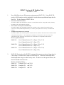
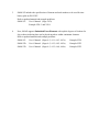
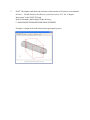
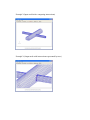
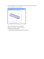
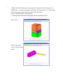
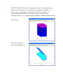
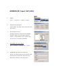
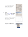
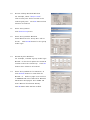
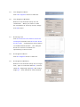
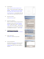
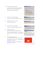
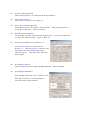
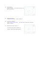
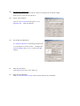
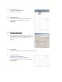
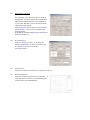
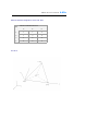
SMAP Version 6.51 Update Note
April 1, 2006
1.
GEN-3D (SMAP-3D pre-processing program) includes the following new features:
C
Generating Straight/Circular Line Block
Each block can be specified as either straight or circular line block.
C
Specifying Different Material Numbers for Each Block
Different material numbers can be specified for each block.
Some designated material
numbers within a block can be removed.
C
New Input Data Format for Block Coordinate and Block Data
Input data formats have been changed for block coordinate and block data.
Refer to updated manual.
SMAP-3D:
2.
GEN-3D User’s Manual (Pages 5-67 to 5-73)
ADDRGN-2D (SMAP-S2/2D pre-processing program) includes the following new
features:
C
Exceptional Material Numbers for Editing
For IEDIT = 2 and 3 in Card 3.3, those elements with material numbers of MC, MB, and MT will
not be influenced by editing.
C
Material Number for MATold
For MTYPE = 4 and -4 in Card 3.3.5.4.1, program automatically assigns MATold = MATNO +1
if MATNO is positive and program takes initial value for MATold if MATNO is negative.
C
Boundary Conditions for Base Mesh
Left, right, top and bottom boundary conditions for base mesh in Card 4.1 can be specified
as either free or roller.
Refer to updated manuals.
SMAP-S2:
ADDRGN-2D User’s Manual (Pages 6-4 and 6-14)
SMAP-2D:
ADDRGN-2D User’s Manual (Pages 6-4 and 6-14)
3.
For IEDIT = 2, 3, -2 and -3 in ADDRGN-3D Card 3.3, those elements with material
numbers of MC, MB, and MT will not be influenced by editing.
Refer to updated manual.
SMAP-3D: ADDRGN-3D User’s Manual (Page 6-18)
4.
SMAP-S2/2D/3D (SMAP-S2/2D/3D main-processing program) includes the following
new features:
C
Exceptional Continuum Material Numbers for Embedding Truss
Continuum material numbers (MATP1 , MATP2 and MATP3 )
in Card 7.3 are not allowed to
embed truss element.
C
Element Activity Based on Material Property Number
Element activity in Card Group 8 can be specified based on material property numbers.
Refer to updated manuals.
SMAP-S2:
SMAP-S2 User’s Manual (Pages 4-42 and 4-44)
SMAP-2D: SMAP-2D User’s Manual (Pages 4-81 and 4-83)
SMAP-3D: SMAP-3D User’s Manual (Pages 4-67 and 4-69)
SMAP Version 6.50 Update Note
November 5, 2005
1.
Now, SMAP has its own 3D post-processing program (PLOT-3D). Using PLOT-3D,
results of 2d/3d analyses can be graphically viewed without any additional input data for
Post File. The key features of PLOT-3D are:
C
Plot finite element meshes
It reads the Mesh File described in Section 4.3 and plots meshes along with node, element,
boundary code, and material numbers.
C
Plot results of analyses automatically
It reads the Mesh File and SMAP output files and then, with no input for Post File, plots
contours of stress/strain/displacement, iso surface, principal stress vectors, and deformed
shapes.
C
Compute intersections of surfaces
It reads the Mesh File containing shell elements for 3D surfaces and shows the locations of the
computed intersections.
The computed coordinates of intersections are saved in a file
“Intersection.dat” which can be used for the construction of complicated 3D meshes.
Refer to updated manuals.
SMAP-S2:
User’s Manual Section 3.3.4 (Pages 3-39 to 3-53)
User’s Manual Section 3.4.3 (Page 3-57)
SMAP-2D:
User’s Manual Section 3.3.4 (Pages 3-39 to 3-53)
User’s Manual Section 3.4.3 (Page 3-57)
SMAP-3D:
User’s Manual Section 3.3.4 (Pages 3-52 to 3-66)
User’s Manual Section 3.4.3 (Page 3-70)
2.
PLOT-XY (Previously called PLTXY) automatically generates preselected input data for
Card Group 12 based on user’s input in Card Group 10. Then users can modify these
default input data using text editor as they want. In order to use this special feature, the
Post File should contain no data.
Refer to example problems..
SMAP-S2:
Example VP8-2 and VP9-1
SMAP-2D:
Example VP1
and VP13
SMAP-3D:
Example VP1
and VP9
3.
SMAP-S2 includes the specification of element and node numbers to be used for time
history plots by PLOT-XY.
Refer to updated manual and example problems.
SMAP-S2:
User’s Manual (Page 4-47a)
Example VP8-2 and VP9-1
4.
Now, SMAP supports Embedded Truss Elements with explicit degrees of freedom for
slip so that reinforcing bars can be placed anywhere within continuum elements.
Refer to updated manuals and example problems.
SMAP-S2:
User’s Manual (Pages 4-5, 4-11, 4-43, 4-43a)
Example VP14
SMAP-2D:
User’s Manual (Pages 4-5, 4-12, 4-82, 4-82a)
Example VP22
SMAP-3D:
User’s Manual (Pages 4-5, 4-12, 4-68, 4-68a)
Example VP22
5.
PLOT-3D computes and shows the locations of intersections of 3d surfaces as mentioned
in Note 1. For this feature to be effective, you need to select “Yes” for “Compute
Intersection” in the PLOT-3D Setup.
Refer to Example1 and Example2 in the directory;
C:\SMAP\SMAP3D\EXAMPLE\PRESMAP\INTERSEC
Example 1 (Output mesh with intersections represented by truss)
Example 2 (Input mesh before computing intersections)
Example 2 (Output mesh with intersections represented by truss)
6.
GEN-3D (SMAP-3D pre-processing program) can place the generated 3d structures
in any specified direction as shown below.
Refer to updated manual and example problem.
GEN-3D User’s Manual (Pages 5-67 and 5-68)
Example problem in the directory
C:\SMAP\SMAP3D\EXAMPLE\PRESMAP\GEN-3D\EX5
7.
CROSS-3D (SMAP-3D pre-processing program) is improved in mesh refinement for
MODELNO = 2 so that it can generate reasonably well shaped meshes even if the height
of the small tunnel is much smaller than that of the large tunnel.
Refer to example CR-M2-1 in the directory
C:\SMAP\SMAP3D\EXAMPLE\PRESMAP\CROSS-3D\MODEL2\M2-1
Whole meshes
Meshes representing
cores of small and large
tunnels
8.
ADDRGN-3D (SMAP-3D pre-processing program) includes two additional features:
C
Changes material numbers so as to match those in continuum blocks (IEDIT = -3)
C
Adds two layers of shell elements with joint elements in-between (IEDIT = 5)
Refer to updated ADDRGN-3D User’s Manual (Pages 6-18 and 6-23) and
Example for IEDIT = 5 in C:\SMAP\SMAP3D\EXAMPLE\ADDRGN\ADD-3D\MOD-5
Whole Meshes
Shell and Joint Elements
generated by ADDRGN-3D
9.
SMAP-2D / 3D supports Ko condition for Engineering Model (MODELNO = 10) and
Duncan & Chang Hyperbolic Model (MODELNO = 12).
Refer to updated manuals.
10.
SMAP-2D:
User’s Manual (Page 4-34)
SMAP-3D:
User’s Manual (Page 4-33)
SMAP-S2 / TUNA can consider hydrostatic ground water pressures below water table.
Refer to updated manual and example problem.
SMAP-S2:
User’s Manual (Pages 4-21 and 4-22)
TUNA:
User’s Manual (Page 4-3)
Example EX1-1.DAT in C:\SMAP\TUNA\EXAMPLE\EX1\EX1-1
11.
TUNA Plus supports Hoek and Brown Material Model for in situ rock mass.
Refer to updated manual and example problem.
TUNA Plus: User’s Manual (Pages 4-6 and 4-9)
Example EX1-1.DAT in the directory
C:\SMAP\TUNAPLUS\EXAMPLE\EX1\EX1-1
12.
SMAP automatically creates a sub directory Temp under current working directory.
All intermediate scratch files are saved in this sub directory. Consequently, to run
SMAP programs manually, you need to move to this Temp directory.
Refer to updated manual.
SMAP-S2:
User’s Manual (Pages 3-2 and 3-59)
SMAP-2D:
User’s Manual (Pages 3-2 and 3-59)
SMAP-3D:
User’s Manual (Pages 3-2 and 3-72)
TUNA:
User’s Manual (Pages 3-2 and 3-15)
TUNA plus:
User’s Manual (Pages 3-2 and 3-19)
13.
SMAP provides debug information during execution of main-processing program
(solver). This information is useful for tracing run time errors, extracting convergence
status, and checking elapsed time.
Refer to updated manual.
14.
SMAP-S2:
User’s Manual (Page 3-60)
SMAP-2D:
User’s Manual (Page 3-60)
SMAP-3D:
User’s Manual (Page 3-73)
TUNA:
User’s Manual (Page 3-16)
TUNA plus:
User’s Manual (Page 3-20)
SMAP automatically renumbers nodes to reduce bandwidth.
The old input parameter NBAND is replaced by IQUAD. If IQUAD = 1, all linear
elements are automatically transformed into quadratic elements. This powerful new
feature will be available for Version 6.6.
Refer to updated manual.
SMAP-S2:
User’s Manual (Pages 4-15 and 4-15a)
SMAP-2D:
User’s Manual (Page 4-15)
SMAP-3D:
User’s Manual (Page 4-15)
SMAP Version 6.13 Update Note
March 22, 2004
1.
SMAP-S2 / 2D / 3D supports IUNIT = 4 in Card Group 11 of PLTDS plot.
When IUNIT = 4 is specified, post processing program PLTDS reads FORCE,
LENGTH, and TIME units from the file UNIT.DAT in the directory
C:\SMAP\CT\CTDATA.
2.
GROUP.POS which can be obtained by executing ADDRGN-2D contains
general draft forms of SMAP-S2 / 2D post file input. Users can modify this
file appropriately and rename it. Note that Card Group 11 of GROUP.POS
uses IUNIT = 4 so that consistent unit is read from the file UNIT.DAT for
PLTDS plot.
SMAP Version 6.12 Update Note
December 5, 2003
1.
Graphical User Interface (GUI) is available for creation or modification of
ADDRGN-2D input data in building user-defined curves and material zones
(IEDIT = 4). Refer to notes for “ADDRGN-2D Input GUI (AIG)” and
example problems: ADD2D-7.DAT, ADD2D-8.DAT, and ADD2D-9.DAT.
In addition to easy mesh generation features, AIG can be used to specify
element activity data for main file and graphical data for post file.
Execution of ADDRGN-2D generates three output files:
GROUP.MES:
Mesh file
GROUP.MAN:
Main file containing element activity
GROUP.POS:
Post file
2.
SMAP-S2 / 2D / 3D supports linearly distributed surface traction given as
element nodal intensities or functions of global coordinates.
Refer to updated manuals and example problems in the directory
C:\SMAP\SMAP2D\EXAMPLE\SMAP\NATM
SMAP-S2:
Pages 4-27 and 4-27a
Example S2-1-L.DAT
SMAP-2D:
Pages 4-65 and 4-65a
Example 2D-1-L.DAT
SMAP-3D:
Pages 4-64, 4-64a and 4-65a
Example 3D-2E-L.DAT
3.
SMAP-S2 / 2D / 3D supports the change of tangent Young’s modulus as a
function of time. Refer to updated manuals and example problems.
SMAP-S2:
Page 4-37
Example VP13-6.DAT (Beam)
SMAP-2D:
Page 4-75
Example VP21-6.DAT (Beam)
SMAP-3D:
Page 4-66
Example VP21-2.DAT (Shell)
Example VP21-3.DAT (Beam)
SMAP-S2 / 2D / 3D supports “NEL1 -NEL2" generation feature for the
specification of element activity data in Card Group 8. For element
numbers from NEL1 to NEL2 to have the same active and deactive steps,
prefix negative sign to NEL2. For example,
NEL1
NAC1
NDAC1
-NEL2
NAC1
NDAC1
Refer to example problems.
SMAP-S2:
Example VP6-2.DAT
SMAP-2D:
Example VP16-1.DAT
SMAP-3D:
Example VP14-1.DAT
4.
5.
PLTDS supports plotting deformed shapes based on element numbers.
In Card Group 11.4.5, prefix negative sign to NSR for element based deformed
shape plot.
-NSR
JCR NJR
ICR
NIR
where
NSR:
Starting element number for row plot
JCR:
Element number increment in a row
NJR:
Number of elements in a row
ICR:
Element number increment for next row
NIR:
Total number of rows
Example: C:\SMAP\SMAP2D\EXAMPLE\SMAP\NATM\2D\2D-1\2D-1.DAT
6.
TUNA Plus supports straight line segments and removal of material regions.
In Card Group 3.4.3 and 3.4.4, the value of Young’s modulus (E) determines
these additional features:
For E = 0
3 straight line segments connecting (X1,Y1) through (X4,Y4)
will be built. If X3 = 1.0E+30, only the first line segment will
be built.
For E = -1
Materials in this region will be removed. If X4 = 1.0E+30,
a triangle consisting of the first 3 apexes will be removed.
7.
SMAP-S2 / 2D / 3D supports “Automatic Removal of Deactive Elements for
NPTYPE = 2 and 6 in PLTDS Plots” so that users can specify all continuum
elements using NGROUP = 0. Note that post-processing program PLTDS
identifies deactive elements based on ACDAC.DAT and CYCLE.DAT
files in the working directory. ACDAC.DAT contains element activity
information and CYCLE.DAT contains information relating Step No to Time.
SMAP-S2 does not generate CYCLE.DAT since Step No is the same as Time.
Refer to example problems.
SMAP-S2:
Example VP6-3.DAT
SMAP-2D: Example VP16-2.DAT
SMAP-3D: Example VP14-2.DAT
8.
SMAP-S2 / 2D / 3D supports “Contour Plots of Yield Flag (NCTS = 25) for
NPTYPE = 6 in PLTDS Plots”. Plastic zones have the value of 1 and
elastic zones have the value of 0.
Refer to example problems.
SMAP-S2:
Example VP1-3.DAT
SMAP-2D: Example VP4-2.DAT
SMAP-3D: Example VP4-3.DAT
9.
TUNA Plus includes “AIG for USLAYER.DAT” in Run menu.
“AIG for USLAYER.DAT” generates the file USLAYER.DAT using GUI.
USLAYER.DAT contains the coordinates of User Specified Soil / Rock Layers
in Card Group 3.4. The original coordinates specified in Card 3.4.2 will be
replaced by those coordinates in USLAYER.DAT. The procedure to use
“AIG for USLAYER.DAT” in TUNA Plus is the same as that illustrated in
Steps 5 through 22 for Note 1.
Refer to example problem EX10.DAT.
ADDRGN-2D Input GUI
[AIG]
ADDRGN-2D Input GUI (AIG)
1.
SMAP
Start -> Programs -> SMA P -> Smap
2.
SMAP Program Menu
Selec t SMAP-2D radio bu tton and then click
OK button
3.
W orking Directory
Working directory should be the existing
directory where all the output files are
saved.
Click the disk d rive, double-click
the direc tory, and then OK bu tton .
4.
ADDRGN-2D Input Menu
Run –>Addrgn –> Addrgn-2D –> Input
5.
ADDRG N-2D Input File Window
When you create input file for the first time,
select New for Inp ut File, Base M esh for
Mesh File, and then click OK button.
6.
Base Mesh Window
As an ex am ple, consider a Base M esh
wh ich is 30 me ters in w idth, 2 0 m eters in
height and 0.5 m eter in element size.
Click OK button when finished.
7
Plot Mesh
Double-click the first item “FINITE ELEMENT
MESHES” in the list box.
Click OK button
when finished.
8.
Base Mesh Plot
30m x 20m base m esh w hich is specified in
Step 6 will be shown on the screen along
wit h grid and tick m arks.
9
Mouse Pickup Menu
To access Mou se Pickup M ethod, select
Draw-Style -> Mouse Pickup
10.
Mouse Pickup Method Window
For exam ple, select “Sn ap to G rid”.
T hen m ou se p oin t w ill b e m oved to the
nearest grid point.
Click OK button when
selection is finished.
11.
Start Group Menu
Click Start Group menu.
12.
Start Group Initial Window
Initial blank form for Group No 1 will be
shown.
Click MTYPE button for the group
mod el type.
13.
MTYPE O ption Window
For example, consider a group model type
MTYPE = 3 which will replace the material
num ber within the closed loop.
Click OK
button when selection is finished.
14.
Start Group Window for MTYPE = 3
Click Refresh bu tton to rese t fields for
MT YPE = 3 .
Refer to page 6-10 and 6-11
in AD DR GN -2D User’s M anu al for Ma terial
Parameters and page 4-83 in SMAP-2D
User’s Manual for Element Activity.
Click OK button when the form is filled.
15.
Line Segment Menu
Click Line Segment menu to draw line.
16.
Line Segment Window
Default is set as Mouse Pickup for line
coordinates. When you want to lo cate
the coo rdina tes of a line by m ouse , simp ly
click OK button.
17.
Drawing Line
Click the mouse at the location where the
line begins and then click the m ous e w here
the line ends.
A straight line will be drawn
on the Base Mesh W indow.
The exa m ple
shows a 10 m eter horizontal line
represen ting a tunn el invert.
18.
Arc Segment Menu
Click Arc Segment menu to draw arc.
19.
Arc Segment Window
Default is set as Mouse Pickup for arc origin.
First , type in horizon tal radius Rx, vertical
radius Ry, beginning angle Qb, and ending
angle Qe.
Click OK button when finished.
20.
Draw ing Arc
When you press dow n and hold m ouse
button, an arc will be drawn on Base Mesh
Window .
Drag the mou se to the location
wh ich will be arc origin an d then release
the mouse button. Th e ex am p le sh ow s 5 m
radius half circle representing tunnel arch.
21.
End Group Menu
Click End Group menu.
22.
End Group Window
When you want to finish group generation
and save in a file, click “Finish and Save
Output” radio button, type in output file
n am e, and click OK butto n.
Note th at this
outp ut file is to be u sed as the inp ut file to
the ADDRGN-2D Program.
23.
Close PLTDS.
ADDRGN-2D Execute Menu
Run –> Addrgn –> Ad drgn-2D -> Execute
24.
Open Input File
Click Browse button for input file.
25.
File Open W indow
Double-click the inpu t file which you have
prepared for ADDRGN-2D. For exa m ple,
ADDRG N.NEW which you have created in
Step 22.
26.
Mesh Plot Option Window
Click OK bu tton wh en selection is finis hed .
Refer to pa ge 3-18 in SM AP -2D Us er’s
Manual for detailed description.
27.
Program Running Message
Please wait wh ile th is m essa ge is sho wn .
28.
PRESM AP Mesh Plot Option
Click Yes butto n to plo t
29.
Program Running Message
Please wait while this message is shown.
30.
PLTDS Plotting List
Select an item from the U nplotted List
window and click OK bu tton .
For example,
you can select the first item for finite element
plot.
31.
Finite Element Mesh Plot
The selected plot item in the previous step
wil l be sh ow n on the screen .
Outpu t files are
GROUP.MES: Mesh file
GROUP.MAN: Ma in file for elem ent ac tivity
GROUP.POS:
Post file
Modifying Existing AIG File
32.
Adding Additional Groups
Follow Steps 1 through 4.
At Step 5, select Old for Input File
and click Browse button to open AIG file.
33.
File Open W indow
Double-click the inpu t file which you have prepared for ADDRGN-2D.
In this example, we are using ADDRGN .NEW which was created in Step 22.
34.
Base Mesh Window
Information about base mesh will be shown
on the Base Mesh W indow.
35.
Plot Mesh
As for Step 7, double-click the item “FINITE ELEMENT MESHES” in the list
box.
36.
Click OK button.
Click OK button when finished.
Group No 1 o n Base Mesh
A Group No 1 representing a tunnel section
will be show n on the 3 0 m x 20 m base
mesh.
37.
Mouse Pickup Method
Follow Steps 9 and 10 to select Mouse Pickup Method.
38.
Start Group Menu
Click Start Group menu as in Step 11.
39.
Start Group Initial Window
Initial blank form for Group No 2 will be shown.
the grou p m ode l type.
40.
MTYPE O ption Window
For example, consider a group model type MTYPE = 2 which will represent
an open line element group.
41.
Click MTYPE button for
Refer to Step 12.
Refer to Step 13.
Start Group Window for MTYPE = 2
Click Refresh button to rese t fields for
MT YPE = 2 .
Click Description button for the
description of material parameters and
elem ent ac tivity.
Click OK button when the
form is filled.
42.
43.
Arc Segment Menu
Click Arc Segment menu to draw a straight radial line.
Arc Segment Window
As a straigh t radial line, let’s consider a rock
bolt wit h a le ng th of 5 m at 60 deg rees.
Click OK button when finished.
Refer to Step 18.
44.
Draw ing Arc
Refer to Step 20.
The exam ple show s a rock
bolt at 60 deg rees.
45.
46.
End Group Menu
Click End Group m enu .
Refer to Step 21.
End Group Window
Selec t “Generate New Group”.
Click OK button to generate next group.
Refer to Step 22.
47.
Adding Group No 3 and 4
To generate rock bolts at 90 and 120
degrees, repeat Steps 38 through 46.
48.
Modifying a Segment
For example, let’s assume that we w ant to change the rock bolt length
from 5 m to 7.5 m for Gro up No 3 .
49.
Start Group Menu
Type in 3 for Group No and type in 1 for
Segment No.
50.
Click OK button.
Arc Segment Window
Arc Segmen t Window containing Segment No
1 of Group No 3 will be shown.
Change the
Vertical Radius (Ry) to 12 .5 m and click OK
button.
51.
End Group Menu
Click End Group m enu as in Step 21.
52.
End Group Window
Selec t “Generate New Group” and click OK button as in Step 46.
53.
Refreshing Plot
To reflect the modifications,
select Plot –> Replot
54.
Modified View
A new plot with upd ated information for
Segment No 1 in Group No 3 will be
displayed.
55.
Making a Null Group
For example, let’s make the Grou p N o 2 n ull.
Click Start Group menu, type in 2 for Group
No, select MTYPE = 6 and then click OK
button.
56.
End Group
Follow the same procedure as in Steps 51 and 52.
57.
Refreshing Plot
To reflec t the m odificatio n,
select Plot –> Replot as in Step 53.
A ne w p lot with the G roup No 2 mis sing will
be dis played.
58.
Replacing a Group
For example, let’s assume that we w ant to
completely rewrite Group No 4 to represent a
utility tunnel with a radius of 2.5 m located at
7.5 m to the left and 7.5 m to the top from the
origin of the arch tunnel.
Click Start Group menu, type in 4 for Group No,
select MTYPE = 1, fill in rest of columns, and
click OK button.
It should be noted that Segment No in this Start
Window should be 0.
59.
Arc Segment
Click Arc Se gm ent m enu as in Step 18.
Fill the dimen sions of utility tunnel on the
Arc Segmen t Window as sh ow n.
Click OK button.
60.
End Group
Follow the same procedure as in Steps 51 and 52.
61.
Refreshing Plot
Follow the sam e pro ced ure a s in S tep 5 3. A
new plot with Group No 4 representing the
utility tunnel will be displayed.
62.
Saving Modification
To save all the modifications for AIG file, follow the same procedure as
described in Steps 21 and 22.
63.
Generating Finite Elemen t Mesh
To generate and plot the finite element
mesh corresponding to the AIG file described
in Steps 32 through 62, follow the Steps 23
through 31.
SMAP-S2 Version 6.1 Update
SMAP-S2 User's Manual
Input Data and Definitions (Main File)
Card
Group
5
4-27
5.5
5.5.1
NUMEST
NUMEST
Nunber of element surfaces where
tractions are specified. (max=3000)
If NUMEST =0, go to Card Group 6.
5.5.2 .1
NUMEST + NEL, KP, KH, KD, a0 , a1 , a2
*
-
-
-
- - -
-
.
-
-
-
- -
-
-
NEL
Element number
KP
Element surface designation number
KH
Load history number specified in Card
10.4. If KH=0, constant static
For Each Element Surface
Element Surface Traction
Continuum Element
Cards
pressure/traction vector is acting all
the time.
KD =0
Uniformly distributed traction vector is
defined in local coordinate system
PNn = a0
=1
Px = a1 Py = a2
Uniformly distributed traction vector is
defined in global coordinate system.
PNn = a0
PX = a1 PY = a2
PNn is static normal pressure
(Compression is positive)
4-27a
SMAP-S2 User's Manual
Input Data and Definitions (Main File)
Card
Group
5
5.5.2 .1
=2
Linearly distributed static normal
pressure
Pn1 = a1 at I1 N Pn2 = a2 at I2 N
=3
Linearly distributed surface traction qX
defined in global coordinate system.
For Each Element Surface
Element Surface Traction
Continuum Element
qX1 = a1 at I1 N qX2 = a2 at I2 N
=4
Linearly distributed surface traction qY
defined in global coordinate system.
qY1 = a1 at I1 N qY2 = a2 at I2 N
=5
Static normal pressure PNn is given as
a function of global X and Y coordinate
PNn = a0 + a1 X + a2 Y
=6
Global surface traction qX is given as
a function of global X and Y coordinate
qX = a0 + a1 X + a2 Y
=7
Global surface traction qY is given as
a function of global X and Y coordinate
qY = a0 + a1 X + a2 Y
Refer to description in the following
page for definition.
4-37
SMAP-S2 User's Manual
Input Data and Definitions (Main File)
Card
Group
6
6.4
6.4.1 .1
NTNB
NTNB
Number of different material property
(max=50)
6.4.1 .2.1
MATNO, MODELNO, NEHNO
MATNO
Material number
MODELNO
Material model number
NEHNO
Young's modulus load
For Each Material
in Card 10.4
Material Property Data
For NBLT=1 (User-defined Cross Section)
Beam Element
history number specified
SMAP-2D Version 6.1 Update
SMAP-2D User's Manual
Input Data and Definitions (Main File)
Card
Group
5
4-65
5.7
5.7.1
NUMEST
NUMEST
Nunber of element surfaces where tractions
are specified. (max=3000)
If NUMEST=0, go to Card Group 6.
5.7.2 .1
NUMEST + NEL, KP, KH, KD, a0 , a1 , a2
* - - - - - - - - - -
Cards
For Each Element Surface
Element Surface Traction
Continuum Element
. - - - - - - - - - -
NEL
Element number
KP
Element surface designation number
KH
Load history number specified in Cards
9.2.3.1 through 9.2.3.5.
If KH=0, constant static pressure/
traction vector is acting all the time.
KD =0
Uniformly distributed traction vector is
defined in local coordinate system.
PNn = a0
=1
Px = a1 Py = a2
Uniformly distributed traction vector is
defined in global coordinate system.
PNn = a0 PX = a1 PY = a2
PNn is static normal pressure.
(Compression is positive)
4-65a
SMAP-2D UserNs Manual
Input Data and Definitions (Main File)
Card
Group
5
5.7
5.7.2 .1
=2
Linearly distributed static normal pressure
Pn1 = a1 at I1 N
=3
Pn2 = a2 at I2 N
Linearly distributed surface traction qX
defined in global coordinate system.
qX1 = a1 at I1 N
=4
qX2 = a2 at I2 N
Linearly distributed surface traction qY
defined in global coordinate system.
For Each Element Surface
Element Surface Traction
Continuum Element
qY1 = a1 at I1 N
=5
qY2 = a2 at I2 N
Static normal pressure PNn is given as a
function of global X and Y coordinates.
PNn = a0 + a1 X + a2 Y
=6
Global surface traction qX is given as a
function of global X and Y coordinates.
qX = a0 + a1 X + a2 Y
=7
Global surface traction qY is given as a
function of global X and Y coordinates.
qY = a0 + a1 X + a2 Y
Note:
Element surface tractions are not
available for KS=-1 (High Explosive Solid
Element). Refer to description in the
following page for definition.
4-75
SMAP-2D UserNs Manual
Input Data and Definitions (Main File)
Card
Group
6
6.4
6.4.1 .1
NTNB
NTNB
Number of different material property
(max=50)
6.4.1 .2.1
MATNO
Material number
MODELNO
Material model number
NEHNO
Young's modulus multiplication
factor history number in Card
For Each Material
Group 9.2.3
Material Property Data
For NBLT=1 (User-defined Cross Section)
Beam Element
MATNO, MODELNO, NEHNO
SMAP-3D Version 6.1 Update
4-64
SMAP-3D User's Manual
Input Data and Definitions (Main File)
Card
Group
5
5.7
5.7.1
NUMEST
NUMEST
Nunber of element surfaces where tractions
are specified. (max=3000)
If NUMEST=0, go to Card Group 6.
5.7.2 .1
NUMEST + NEL, KP, KH, KD, a0 , a1 , a2 , a3
Cards
* - - - - - - - - - -
NEL
Element number
KP
Element surface designation number
KH
Load history number specified in Cards
9.2.3.1 through 9.2.3.5.
For Each Element Surface
Element Surface Traction
Continuum Element
. - - - - - - - - - -
If KH=0, constant static pressure/traction
vector is acting all the time.
KD =0
Uniformly distributed traction vector is
defined in local coordinat system.
PNn = a0 Px =a1 Py =a2 Pz=a3
=1
Uniformly distributed traction vector is
defined in global coordinate system.
PNn = a0 PX =a1 PY =a2 PZ =a3
PNn is static normal pressure.
(Compression is positive)
=2
=3
Linearly distributed static normal pressure
Pn4 = a0 at I4 N
Pn1 = a1 at I1 N
Pn2 = a2 at I2 N
Pn3 = a3 at I3 N
Linearly distributed surface traction qX
defined in global coordinate system.
qX4= a0 at I4 N
qX1= a1 at I1 N
qX2= a2 at I2 N
qX3= a3 at I3 N
SMAP-3D User's Manual
Input Data and Definitions (Main File)
Card
Group
5
4-64a
5.7
5.7.2 .1
=4
Linearly distributed surface traction qY
defined in global coordinate system.
=5
qY4 = a0 at I4 N
qY1 = a1 at I1 N
qY2 = a2 at I2 N
qY3 = a3 at I3 N
Linearly distributed surface traction qZ
=6
qZ4= a0 at I4 N
qZ1= a1 at I1 N
qZ2= a2 at I2 N
qZ3= a3 at I3 N
Static normal pressure is given as a
function of global X, Y and Z coordinate
PNn = a0 + a1 X + a2 Y + a3 Z
For Each Element Surface
Element Surface Traction
Continuum Element
defined in global coordinate system.
=7
Global surface traction qX is given as a
function of global X, Y and Z coordinate
qX = a0 + a1 X + a2 Y + a3 Z
=8
Global surface traction qY is given as a
function of global X, Y and Z coordinate
qY = a0 + a1 X + a2 Y + a3 Z
=9
Global surface traction qZ is given as a
function of global X, Y and Z coordinate
qZ = a0 + a1 X + a2 Y + a3 Z
Note:
Element surface tractions are not
available for KS=-1 (High Explosive
Solid Element). Refer to description in
the following page for definition.
SMAP-3D User's Manual
Element Surface Designation and Local Axes
KP
4 Node Tetrahedral Element
I1 '
I2 '
I3 '
1
1
2
3
2
1
3
5
3
1
5
2
4
2
5
3
For KP=1
4-65a
4-66
SMAP-3D User's Manual
Input Data and Definitions (Main File)
Card
Group
6
6.1
NBEAM
NBEAM
Total number of beam element
If NBEAM=0, go to Card Group 7.
6.2
NBMST
NBMST
Use NBMST=1
6.3
NTNB
NTNB
For Each Msterial
Beam Element
6.4
Number of material property set for beam element
6.4.1
MATNO, MR, NEHNO
MATNO
Material number
MR
Moment release flag
=0
No hinge
=1
Hinge at node I
=-1
Hinge at node J
=2
Hinge at node I and J
NEHNO
Young's modulus multiplication
factor history number in Card
Group 9.2.3
6.4.2
A, WL, RHO, E, G, J, Iy , Iz
A
Cross section area
WL
Weight per unit length of beam
RHO Mass density
E
Young's modulus
G
Shear modulus
J
Torsional moment of inertia
Iy
Moment of inertia about member y axis
Iz
Moment of inertia about member z axis