1
ARTICLE IN PRESS
Computers & Geosciences ] (]]]]) ]]]–]]]
www.elsevier.com/locate/cageo
Mirone: A multi-purpose tool for exploring grid data$
J.F. Luis
CIMA, Universidade do Algarve, Campus de Gambelas, 8000-117 Faro, Portugal
Received 15 October 2005; received in revised form 5 May 2006; accepted 26 May 2006
Abstract
Mirone is a Windows MATLAB-based framework tool developed by the author that allows the display and
manipulation of a large number of grid formats through its interface with the Geospatial Data Abstraction Library
(GDAL). Its main purpose is to provide users with an easy-to-use graphical interface to the more popular programs of the
Generic Mapping Tools (GMT) package. In addition it offers a range of tools dedicated to topics in the earth sciences,
including tools for multibeam mission planning, elastic deformation studies, tsunami propagation modeling, earth
magnetic field computations and magnetic Parker inversions, Euler rotations and poles computations, plate tectonic
reconstructions, and seismicity and focal mechanism plotting. The high-quality mapping and cartographic capabilities for
which GMT is renowned is guaranteed through Mirone’s ability to automatically generate GMT cshell scripts and dos
batch files. User-specific requirements that lie outside the current capabilities of Mirone can be met by simple programming
to provide the required functionality.
r 2006 Elsevier Ltd. All rights reserved.
Keywords: Mirone; GMT; Data conversion; Grids; Geomagnetism; Plate tectonics; Geophysics
1. Introduction
Mirone is an open source code written in
MATLABs 6.5 by the author and has been
developed specifically for the purpose of visualizing
and manipulating GMT netCDF grids. GMT
(Wessel and Smith, 1991) is one of the most popular
programs within the scientific community on
account of its mapping capabilities and high-quality
graphics. However, most commercial software
packages ignore this format and products that are
able to read GMT, and to display and manipulate
$
Code available from server at http://w3.ualg.pt/jluis/
mirone/
Tel.: +351 289 800938; fax: +351 289 818353.
E-mail address: [email protected].
0098-3004/$ - see front matter r 2006 Elsevier Ltd. All rights reserved.
doi:10.1016/j.cageo.2006.05.005
GMT grids, are rare. An additional problem that
users face concerns data format. There are presently
tens of different formats for storing gridded data
and imagery data, and accessing data from disparate sources is a common problem. Mirone
minimizes this obstacle through its interface with
the GDAL (www.gdal.org). GDAL is a unifying C/
C++ API for accessing raster geospatial data
released under the MIT Open Source license, which
aims to provide efficient access suitable for use in
viewer applications, and which attempts to preserve
coordinate systems and metadata.
MATLAB is a powerful tool for software
development. The language is easy to learn and
contains a large collection of mathematical functions that facilitate the task of writing complicated
code, including Graphical Users Interfaces (GUIs).
ARTICLE IN PRESS
2
J.F. Luis / Computers & Geosciences ] (]]]]) ]]]–]]]
However, it also has limitations including those
of speed and memory consumption. In order to
circumvent these constraints, almost all substantial
computations involving matrix data in Mirone have
been made with the help of external code written in
C and compiled as mex files. Because the mex files
use scalar programming and employ single precision
or short integer variables in circumstances where
accuracy is not compromised, their memory consumption is reduced to the minimum necessary
whilst the running speed is that of a compiled code.
This paper reports the general characteristics of
Mirone, and describes and explains the program’s
main capabilities and functions. The paper also
provides some example applications to topics in the
earth sciences including elastic deformation, tsunamis, and plate tectonic motions. Aspects of the
future refinement and development of Mirone are
also addressed, including an example of how it can
be extended by programming for particular needs.
The source code and a stand-alone version, which is
a version that does not require MATLAB, are
available at w3.ualg.pt/jluis/mirone.
2. The program design philosophy
Mirone was designed to address many of the
specific needs of those who regularly use gridded
data, but is particularly focused on the fields of
geophysics and earth sciences. It provides comprehensive data visualization and analysis in a userfriendly environment. One of Mirone’s advantages
is that the author is also a user. I have found
that much graphically oriented software obliges
the user to follow a strict procedure that often
requires in-depth study of the accompanying
manual in order to accomplish even simple display
tasks. In Mirone, the user merely loads the grid of
interest (assuming that it belongs to one of the
recognized formats) and views it. Particular attention has been paid in the program to offer the
user the simpler and more often used options first,
and to let the more specific options show up only
when they may be needed to solve a particular
problem.
Since Mirone offers a large number of operations,
it has been designed in a modular fashion. Options
that require input parameters are run from independent windows which, whenever possible, offer
‘‘clever’’ default values. A comprehensive set of
‘‘tooltips’’ and ‘‘helps’’ has been attributed to the
buttons and boxes where data have to be entered, in
order to facilitate the comprehension of each
module’s operation, to the extent that many
modules should not require reference to the manual.
The modular design can be explored further by
users with programming skills, and it is relatively
easy to add new possibilities to the main program,
as demonstrated in Section 7 below.
For the purposes of demonstration or teaching, a
number of datasets have been incorporated covering
topics such as seismicity, active volcanoes, ODP/
DSDP sites, plate boundaries, major cities, and
magnetic isochrons of the world’s oceans. These
datasets are not purely static but contain relevant
information associated with various items. For
example, right clicking on a plate boundary segment
informs the user about neighboring plates as well as
the opening rate and direction.
3. Starting the program
Upon starting the user is presented with Mirone
in its basic form, which is a simple bar containing
various menus. See Fig. 2 for an example of a
Mirone window with data already displayed.
Activities are initiated by using these menus.
Although Mirone has pre-defined defaults it is very
important that the user understand what these
defaults mean and do. The first time the program
is used the user is strongly advised to press the
button with hammers icon. This icon opens the
preferences window (Fig. 1). The meanings of those
settings are:
Use new GMT netCDF grid format . Starting with
GMT version 4.1, a new type of COARS-compliant
GMT net CDF grids was introduced. While this
change is transparent to users, the new grid format
will not be recognized by previous GMT versions.
Grid coordinates . Select Geographic (default) if
working with a grid whose coordinates are longitude and latitude, otherwise select Cartesian. This
is an important setting because some operations,
such as measuring, depend on the grid coordinate
system.
Grid Max size . In order to perform grid manipulations, Mirone stores the original grid in the
computer’s memory (in single precision). This is the
maximum size in Mb that a grid can occupy in the
computer’s memory. This does not mean that larger
grids/images cannot be processed, it means that if
they exceed the size value they will be re-read from
disk as required. The user must decide a reasonable
value for this parameter based on the capabilities of
ARTICLE IN PRESS
J.F. Luis / Computers & Geosciences ] (]]]]) ]]]–]]]
Fig. 1. Parameter configuration window.
the computer being used. Grid size is computed as:
n_rows n_columns 4/(1024 1024). (Note: Mirone makes most of its heavy computation using
external mex files that use scalar single and double
precision arithmetic. However, some operations
may be performed with MATLAB operators using
imply double precision, which takes twice as much
memory. When image files are being used, however,
this rule does not apply.)
Swath ratio . When performing a multibeam
planning, the swath width coverage as a function
of the water depth needs to be known. When the
first track is started by the user, a question will be
made concerning whether the current value is to be
used, or whether it should be changed.
Measure units . When computing distances, the
result is presented in the chosen unit. Available
options are nautical miles, kilometers, meters, and
user-defined.
Default ellipsoid . Mirone computes distances on
an ellipsoidal Earth. The list of available ellipsoids
include the 63 GMT-supported ellipsoids plus one
for Mars, which is needed when working with
3
MOLA grids. Users that whish to set a custom
ellipsoid will need to edit the mirone_prefs.m file.
Working directory . To reduce the cumbersome
task of browsing through the directory tree every
time a file needs to be saved, the program uses a
default working directory. Either the full path may
be typed here, or the side button pressed to select a
directory within a new window.
New grids in new window . Many options involve
the computation of a new grid. This parameter
controls whether the newly computed grid is
automatically opened in a new Mirone window (if
this option is checked) or saved on a disk file.
Force insitu transposition . This option helps with
the importation of large grids. Importing grids
involves a conversion that uses matrix transposition, which requires twice the grid size in memory
when a copy is made of the grid to speed importation. The in situ transposition option uses only
the grid size in memory and should be used where
the computer has insufficient memory, although the
importation runs about 10 times more slowly than if
the grid is copied.
When possible save as int16 . Some grids use short
ints (2 bytes) to save disk space. Checking this
option means that, if the grid is saved in the GMT
format, the 2 bytes original density will be retained
(otherwise, it will be saved as floats of 4 bytes). This
is useful, for example, to convert Shuttle Radar
Topography Mission (SRTM) grids into GMT
format.
Default line thickness . This default value is used
for drawing lines, circles or other graphical elements.
Default line color . This default value is used for
drawing lines, circles or other graphical elements
(such as text strings).
For a complete explanation of all options offered
by the program the reader is directed to the user’s
manual.
4. General functionality
By default Mirone automatically detects and
reads all types of netCDF GMT grids as well as
Surfer 6 and 7 grids. Many of the formats
recognized by GDAL may also be accessed through
the File menu. Those include: GeoTIFF DEM,
DTED, USGS DEM, USGS SDTS DEM, Gtopo30, SRTM DEM, Arc/Infos ascii/binary grids,
ENVI, ERDAS. img, GeoTIFF, Grid Exchange
File (GXF from Geosofts), Mars Orbiter Laser
ARTICLE IN PRESS
4
J.F. Luis / Computers & Geosciences ] (]]]]) ]]]–]]]
Altimeter (MOLA) grids, and the common image
formats. When the loaded grid is referenced in
geographical coordinates it is also possible to plot
the netCDF coastlines database (including rivers
and political divisions) provided by GMT. These
include not only the coastlines themselves but also
the rivers and political divisions (country frontiers
and US states). The netCDF coastlines database is
the only currently available non-ASCII vector
format. Other line and point data must be loaded
from ASCII disk files containing x,y coordinates,
one record per line. Multi-segment files, that is a file
where segments are separated by a special record
(the ‘4’ character), are also supported.
When a grid is loaded the Mirone window
expands to accommodate the image derived from
the grid. At the bottom of the window the current
mouse position is displayed in the grid’s coordinates. Clicking and dragging over the image shows
the distance in the selected user units. The generated
image uses a default color map, but more than 100
other color palettes are available by clicking on the
palette icon button to access the palette tool (not
shown here). All palettes may be changed by a
double click over the color bar. This inserts color
markers, which can be dragged to modify the color
map. A second double click deletes the marker. The
Min Z and Max Z fields may be used to impose a
fixed color map between those values. External
GMT color palettes may also be imported or
exported via the File menu.
Another common operation is to show patterns
and fine details in the grid image as revealed by
applying a shading illumination. Mirone offers five
different algorithms for shading illuminations. By
default a mex version of the GMT grdgradient
program is used to do this, but the user can select
any of the five methods from within the control
window. Sun azimuth and elevation (when accepted
by the method) are controlled with the mouse.
The buttons with T, circle, line, rectangle, closed
polygon, and arrow icons permit the user to draw
any of these graphical elements (Fig. 2). Those
elements may be subsequently edited by doubleclicking the selected target. Besides their use as
simple drawings (which may be saved as ascii files)
such elements (in particular the polylines, rectangles, and closed polygons) allow other possibilities.
A polyline, for example, may be used to measure the
distance or azimuths of its individual segments, and
it can be also used to extract and show a savable
grid profile in much the same way as the grdtrack
Fig. 2. Example case: base image was computing by shading
illumination of a GMT bathymetry grid. Dark dots represent
seismicity as imported from an ISC catalog. Triangles correspond
to active volcanoes. Also two logo images were inserted to
demonstrate this facility.
GMT program. Rectangles may be used to limit the
range of one operation to the area delimited by the
rectangle. The Crop Image operation is quite
common in many programs that display image type
files. In Mirone I have extended that concept to
other operations. It is thus possible to extract a subregion of a grid, compute histograms and power
spectrums, determine autocorrelation, apply median
filters, smooth by spline interpolation, fill gaps
(holes) in the grid, set all grid nodes to a constant
value, and utilize a separate tool, also included in
the package, to perform Region Of Interest (ROI)
image processing type manipulations. Furthermore,
the rectangle’s limits may be used to register an
image into another coordinate system. The rectangle corner coordinates are used to compute an affine
transformation that registers the image to the
rectangle’s coordinate system. The closed polygons
also offer the possibility of measuring areas,
cropping grids, and performing ROI manipulations.
The polygonal cropping differs from the rectangular
one in that the grid nodes external to the polygon
are set to not a number (NaN).
Mirone contains a large collection of both
general-purpose operations and discipline specific
modules. Among the first group, generally organized inside the Grid Tools menu, the user may find
interactive tools to drive a selection of GMT
programs, namely:
Grdfilter —filters grids in the time domain using
one of the selected convolution or non-convolution
filters.
ARTICLE IN PRESS
J.F. Luis / Computers & Geosciences ] (]]]]) ]]]–]]]
Grdgradient —computes the directional derivative in a given direction, or the direction (and
the magnitude) of the vector gradient of the
data.
Grdproject —transforms a gridded data set from
a rectangular coordinate system into a geographical
system (or vice-versa) by resampling the surface at
the new nodes.
Grdsample —reinterpolates and creates a new
grid with either a different registration or a new
grid-spacing or number of nodes, and perhaps also a
new sub-region. Interpolation is bicubic or bilinear
and uses boundary conditions.
Grdtrend —fits a low-order polynomial trend to
the grid of interest using (optionally weighted) leastsquares.
Surface and nearneighbor —interpolates randomly space triplets (x,y,z) into a regular matrix (that
can later be saved as a GMT grid).
Other options involve computing histograms,
clipping a grid above and/or below selected planes,
writing a mask grid where non-NaN values are
replaced by the number 1, computing spectra and
autocorrelations, smoothing grids by spline interpolation, computing slope, aspect, and directional
derivatives, and computing a Second Derivative in
the direction of Gradient (SDG). The SDG is the
algorithm recommended by the United Nations
Convention for the Law Of Sea (UNCLOS) to be
used in the determination of the Foot Of continental
Slope (FOS).
The SRTM has obtained elevation data over
most of the globe to generate the most complete
high-resolution digital topographic database of the
planet. It is distributed as 11 DTM tiles of 1 arcsec
for the US territories and 3 arcsecs for the rest of the
world between 561S and 601N. In areas of high
relief, areas covered by water (e.g., rivers, dams, and
natural lakes), and at land-ocean transitions, the
SRTM models commonly display zones of no-data
(grid holes). Although strategies to fill these holes
using coarser data (e.g., from the elevation data
model GTOPO30) could potentially be used, the
coarser resolution may not depict such areas with
sufficient accuracy. Therefore, the Mirone solution
is simply to offer the user the possibility to fill the
holes, which are automatically detected in Mirone,
by either minimum curvature or bilinear interpolation. The resulting processed file may be saved in the
SRTM format.
Given the limited coverage (11 11) of each
individual SRTM tile, it is often desirable to be
5
able to create mosaics. Mirone has a dedicated and
easy-to-use tool to accomplish this task (Fig. 3).
With the SRTM mosaic tool the user first draws a
rectangle to define the ROI. By right clicking on the
rectangle and choosing mesh , yellow quadrangles
corresponding to possible SRTM tiles can be
drawn. A mouse-click on each individual quadrangle searches the previously selected working
directory for existing SRTM files. The square turns
red if the matching file exists, if it does not exist a
warning message is displayed and the square returns
to yellow.
The size of raster datasets grows very quickly.
For example, the General Bathymetric Chart of the
Oceans (GEBCO) 1 min resolution grid contains
445 Mb of data, but the global mosaic of the SRTM
tiles amounts to 1.9 Gb in GeoTIFF DEM format.
This means that the majority of computers owned
by typical users will probably not be able to process
those files at their full resolutions. One way to
circumvent this problem, as used by some software packages, is to use complicated algorithms
that split the entire dataset (if the data format
allows them to) in layers of variable resolution.
Mirone approaches the problem of loading data
from very large grids somewhat differently. With
the File 4open overview tool the user may
inspect the contents of a very large grid without
loading it. What this tool actually does is to read nother rows and columns in order to obtain an
overview grid that is as close as possible to
200 200 rows and columns, and builds a preview image. The user can then draw a rectangular area in order to extract the data at its full
resolution.
Fig. 3. SRTM mosaic tool showing four successful tile selections
and error message displayed when intend SRTM tile could not be
found in indicated directory.
ARTICLE IN PRESS
6
J.F. Luis / Computers & Geosciences ] (]]]]) ]]]–]]]
5. Discipline-specific tools
Mirone contains a range of specific tools for
application to topics in geophysics and earth
sciences. The list of applications cover multi-beam
mission planning, elastic deformation, tsunami
modeling; including travel time estimation, plate
tectonic reconstructions, Euler rotations and Euler
poles computations, magnetic field computations
and magnetic inversions, and seismicity and focal
mechanism plotting. A selection of these tools is
discussed below.
5.1. Elastic deformations
The elastic deformation tools are accessible via
the
Geophysics 4Elastic deformation
menu.
Here, a line or polyline can be imported or drawn
over the image grid. The line is interpreted as the
surface trace of a fault. Right clicking on the line
allows the user options to open new windows in
which can be specified the fault parameters (width,
depth, dip) as well as the movement/deformation to
be simulated.
The two available deformation options are called
Okada and Mansinha (Okada, 1985). The Okada
tool is more general and can be used to simulate coseismic displacement (that can be compared with
GPS measurements) for an initial condition of
the far field tsunami modeling (see below) or to
compute synthetic interferograms. The Okada
window provides help in the form of tooltips when
the mouse rests over individual entry boxes. For a
complete reference to the use of the Okada window
the user should read the RNGCHN program paper
(Feigl and Dupre, 1999). In that original paper, the
RNGCHN code is provided both as a stand-alone
FORTRAN code and as a MATLAB FORTRAN77 mex file. The stand-alone code depends
on some C code to deal with input/output but it is
system dependent (it runs only on Sun and HP
UNIX systems). The mex file, because it is written in
F77, has the limitation of not supporting dynamic
memory allocation. Mirone uses a C version in
which coordinate conversion routines were added.
The Mansinha option computes only the vertical
component of the deformation produced by an
earthquake. The two codes should produce equal
results and trials show this to be the case. In both
Okada and Mansinha , all distances are computed
by projecting the geographical coordinates to
Transverse Mercator with the origin being the
fault’s first point. Fig. 4 presents an example of
using Okada .
5.2. Tsunami modeling
Mirone has two codes to perform tsunami
modeling of propagation and inundation. The
SWAN code (Madder, 2004, rMader Consulting
Co) and the TUNAMI-N2 code (Imamura, 1997).
Both of these codes were converted from FORTRAN to C to allow dynamic memory allocation.
The example presented here uses the SWAN code.
To use this program, the user needs to have two
grids that are exactly compatible (i.e. they must
cover the same region and have the same number of
rows and columns). One of the grids represents the
bathymetry (z positive up) in meters and the other
contains the initial deformation as produced by
the Mansinha or Okada deformation module.
A required parameter file ‘‘swan.par’’ can be found
in the data directory of the root Mirone installation,
which can be used as an example for other cases.
The user must choose between computing the
simulation on specific points, termed ‘‘maregraphs’’
here, and/or on the whole grid region. If the first
option is desired, the stations can be plotted
graphically (using the Plot Stations option), or the
maregraphs’ locations can be imported in an x,y file.
If the simulation is to be performed over the whole
region, then the Compute option is used. A new
window called swan_options will popup where the
final selections are made. See the user’s manual for
further details on using this tool.
Fig. 4. Example of parameter settings used to characterize
movement along a fault and to compute elastic deformation
produced by that movement.
ARTICLE IN PRESS
J.F. Luis / Computers & Geosciences ] (]]]]) ]]]–]]]
5.3. IGRF calculator
The International Geomagnetic Georeference
Field (IGRF) calculator (Fig. 5) is a tool that
computes the value of the total magnetic field (or its
components) for given points. A single point can be
selected either by a mouse click on the world map or
by entering its exact coordinates. Alternatively, a
file can be read and imported that contains the
magnetic data along with longitude and latitude
positions. The user has the option of choosing to
compute the magnetic anomaly (measured total
field minus the IGRF magnitude). Computing the
magnetic anomaly requires knowing the date of
data acquisition, in which case the file reading
function has the ability to decode many date
formats, including text formats. The IGRF model
used is the 10th generation IGRF as agreed in
7
December 2004 by IAGA Working Group V-MOD.
It is valid for dates 1900.0 to 2010.0 inclusive.
The IGRF routine (a C mex file) is also used
within the Parker Direct and Parker Inversion
tools. The first allows the computation of the
magnetic anomaly given a magnetization and
bathymetry map using Parker’s (1972) Fourier
series summation approach. The second performs
the inverse operation, which is the computation of
the magnetization from magnetic field and bathymetry (Parker and Huestis, 1974). This inversion
procedure eliminates the dependency on the shape
and amplitude of the magnetic anomalies with the
distance between the survey altitude and the
seafloor.
5.4. Geographic calculator
This tool is an interface to both the mapproject
and grdproject programs in GMT. It uses a mex
version of these programs and its use is fairly
straightforward. GMT version 4 introduced datum
conversions in mapproject (but not in grdproject )
and shifts that allow conversion between the many
projection systems in use. Currently, only the
Portuguese systems are coded in Mirone. Overall,
this tool frees GMT users from the need to provide
a correct –R for the transformation (potentially
particular hard to know in advance in inverse
transformations), a problem, which has prevented
many users from being able to use grdproject .
5.5. Plate reconstructions
Fig. 5. Illustration of IGRF calculator. Points for which
geomagnetic field is to be computed can be selected by clicking
on image. ‘‘Griding Line Geometry’’ configures grid parameters
necessary to compute a grid, e.g., of total field or magnetic
declination.
This tool lies somewhere between a plate reconstruction demonstration and an application that can
be used to do advanced plate motion work. There
are some dedicated software packages available on
the web that perform plate reconstructions (see for
example www.geodynamics.no/gmap/ngu@gmap/
Geodynamics.htm and links therein). However, the
Mirone plate reconstructions tool is easy to use and
has good functionality. Options can be obtained by
right clicking over the plates. New menus pop up
(see Fig. 6) from which the user can control how the
plates move. By default the program associates a
‘‘movement history’’ to three plates: Iberia, Eurasia,
and Africa. The movement is defined by the poles as
displayed in the window’s bottom left corner. In
addition to the default files, the user can load his/her
own data, including poles files and plates files.
ARTICLE IN PRESS
8
J.F. Luis / Computers & Geosciences ] (]]]]) ]]]–]]]
Fig. 6. Pate reconstruction tool. Reconstructions for particular
times are performed using time slider. Example shows position of
Iberia, Eurasia, and Africa relative to a fixed North America at
90 Ma ago.
The poles used in this program are stage poles
(not finite rotation poles). They have a particular
format as described in the ‘‘rotconverter’’ GMT
program, but example files can be found in Mirone’s
‘‘continents’’ directory. To create new stage poles
files from finite rotations poles, Make stage poles is
clicked and the ensuing instructions followed.
The plates files are simple ascii files with two
columns ‘‘longitude’’ and ‘‘latitude’’. The files may
be multisegments, with the character ‘‘4’’ serving
as the separator. The individual segments may be
closed, in which case the contour is filled; otherwise
they are drawn as lines. The first line in a file must
take the form ‘‘]Name’’, where ‘‘Name’’ is the
plate’s name. This allows the program to associate a
plate and its companion lines with a stage pole. It
also allows other elements (e.g., the 3000 m bathymetric contour) to be added.
Mirone contains several other tools to manage
plate movements. For example, under the Draw
menu the Draw circle 4circle about an Euler pole
opens a window where the user can draw an arc
circle about Euler poles representing the plate’s
present-day movement. Both relative and absolute
plate movement options are available. These arc
circles also let the user compute the velocity vector
(magnitude and direction) at any point along the
circle. This is a useful tool for discovering how one
plate is moving relative to another at a certain
point.
The rotation of magnetic isochrons and the
creation of flow lines are accomplished using the
tool in Geophysics 4euler rotations . Any line
element, either drawn or imported from an ascii file
or point symbol, may be rotated by using either a
stage pole file as described above or a finite rotation
pole. When performing rotations with stage poles,
an age file that controls the ages for which the
rotation is computed is required. For each entry of
that age file (displayed in the window’s listbox) a
new rotated line is plotted in the Mirone main
window. The Magnetic Bar Code button provides
an easy way to select an age sequence using the
geomagnetic polarity scale as reference. If a single
point is selected (using the Pick line from figure
button) instead of a line/polyline, then a single flow
line is plotted. In the Add poles tab the user may
compute the pole that results from a combination of
two finite rotations.
Users who desire to compute their own
Euler
poles
can
do
this
with
the
Geophysics 4compute Euler pole tool. To use this
tool, two lines in the main window are mouseselected by depressing the Pick line from figure
button, and an initial estimate of the Euler pole is
entered. The results of the search algorithm are
graphically displayed every time a better-fitting pole
is found. The process may be rerun using alternative
initial estimates of the Euler pole if satisfactory
results are not obtained with the initial estimate.
6. 3D view and printing
Because Mirone does not use the 3D MATLAB
functions, the program does not offer any built-in
way of displaying graphics in 3D perspective.
Although MATLAB can display in 3D by using
its surface primitive, this consumes a lot of memory
and has poor interactive response. As an alternative,
Mirone uses the IVS Fledermaus free iView3D
viewer (www.ivs.unb.ca/products/iview3d). Fledermaus is a fast, powerful 3D visualization tool
capable of viewing large amounts of data (Fig. 7).
Translations, rotations, and scaling are accomplished by simple mouse controls. For launching
the 3D view all is need is to hit the button with the
eye icon. By launching the 3D view via the ‘‘eye’’
icon (Fig. 2), a temporary fledermaus object
(sd. file) is created and used as an argument for
the iView3D call. As an alternative, the user
may choose to save the fledermaus object in
File 4Save As Fledermaus Objects and later import that object directly from the viewer.
Saving the Mirone display can be achieved
in
three
ways.
The
first
is
through
ARTICLE IN PRESS
J.F. Luis / Computers & Geosciences ] (]]]]) ]]]–]]]
9
Fig. 7. 3D view of a bathymetry grid using Fledermaus free iView3D viewer. Light gray cubes represent seismic events. There are more
epicenters represented but they are hidden behind current figure display. Changing viewpoint with mouse controls will show them. White
line represents coastlines extracted from GMT coastlines database.
File 4Save Image As . . . which saves the current
display image into one of the common image
formats but without including any graphic elements
(e.g., lines, symbols). The second way, through
File 4Export saves both the image and all
elements that may have been added to it in a
screen capture. A third possibility involves generating a GMT cshell script or dos batch file. The
File 4Save GMT script opens a window (Fig. 8)
in which it is possible to fine tune map details such
as size, position on the page, and projection system
used. This tool searches all elements in the display
and decides the best way to reproduce the
display using only GMT commands. For example,
if the image displayed is derived from a GMT
grid illuminated with a shading method from
grdgradient , the script lines will generate an
illumination grid from the original GMT grid and
use ‘‘grdimage’’ with the –I option. If that is not the
case then a screen capture is executed and the image
saved as three R, G, and B grids. The three grids are
then utilized by ‘‘grdimage’’ to rebuild a color
image. Line elements are written on disk and used
by ‘‘psxy’’. However, coastlines, national borders,
Fig. 8. Example of settings used to generate a GMT shell script
to plot contents of a Mirone window. Rectangle, which represents
map’s size, can be dragged over page or have its limits altered.
Any of GMT map projections may be selected.
rivers, and contour lines are not saved. Instead,
appropriate calls to ‘‘pscoast’’ or ‘‘grdcontour’’ are
inserted into the script.
ARTICLE IN PRESS
J.F. Luis / Computers & Geosciences ] (]]]]) ]]]–]]]
10
7. Evolution of Mirone
Mirone is a powerful tool for displaying and
analyzing grid and vector data loaded in a variety of
formats. The Mirone code comprises more than
90,000 lines of MATLAB code and about 30,000 of
C mex code. Due to its modular design, careful
programming, and interface to GMT and GDAL
libraries, the program is able to read large amounts
of data that would otherwise prove impossible if
only MATLAB primitives had been used. Currently,
however, the GDAL and GMT links are weakly
developed. For example, at the moment it is not
possible to load any of the satellite image formats
recognized by GDAL or to import ECW or MrSid
(wavelet-based image compression technologies developed, respectively, by ERMappers and LizardTechs) compressed images. Adding options to do
these tasks is not technically difficult to program,
but great care will need to be taken owing to the
potentially huge size of these types of image files.
GMT itself continues to evolve. The developing
version 5 will be significantly different from
previous versions (although backward compatible).
It will be reborn as a true code library that
programmers will be able to use with little
wrapping code in order to access its full capabilities
(P. Wessel, pers. commun., April 15, 2005).
A MATLAB compatibility layer is also planned,
at which stage Mirone will be able to more fully
explore GMT’s capacities. A full range of map
projections will also be added.
In the meantime adding new options is a
relatively straightforward task. I give a simple
example on how Mirone can be extended to perform
another operation, in this case to add a menu entry
that allows a grid to be flipped upside-down. The
first step is to decide where the new entry will be
added: in the GridTools menu after the Write mask
option is appropriate. The menus are declared
in the mirone_uis.m file. Searching this file for
Write mask reveals lines that read:
uimenuð‘Parent’; h278; . . .
‘Callback’; ‘mironeð‘‘GridToolsGridMask_Callback’’; gcbo; ½; guidataðgcboÞÞ’; . . .
‘Label’; ‘Write Mask’; ‘Tag’; ‘GridToolsGridMask’Þ;
A new uimenu call and a new callback name function are declared, here denoted ‘‘GridToolsFlipUD_Callback’’
uimenuð‘Parent’; h278; . . .
‘Callback’; ‘mironeð‘‘GridToolsFlipUD_Callback’’; gcbo; ½; guidataðgcboÞÞ’; . . .
‘Label’; ‘Flip Up; Down’; Tag’; ‘GridToolsFlipUD’Þ;
Now a new callback function is added to the mirone.m file, and programmed. It would look something like
(without error checking):
function ‘GridToolsFlipUD_CallbackðhObject; eventdata; handlesÞ
% retrieve the arrays stored in figure’s appdata
½X; Y; Z; head ¼ load_grdðhandlesÞ;
% Flip the grid array Up Down
Z ¼ flipudðZÞ;
% Save back the flipped array for future use
setappdataðhandles:figure1; ‘dem_z’; ZÞ;
% Get the image handle
h_img ¼ findobjðhandles:figure1; ‘Type’; ‘image’Þ;
% Flip also the displayed image
setðh_img; ‘CData’; flipdimðgetðh_img; ‘CData’Þ; 1ÞÞ
ARTICLE IN PRESS
J.F. Luis / Computers & Geosciences ] (]]]]) ]]]–]]]
A final aspect of Mirone’s evolution regards its
portability to other operating systems. In its current
form, despite the fact that it is written in MATLAB,
Mirone runs only in Windows. This is a consequence of using many compiled C mex files that are
either self-contained or make calls to the GDAL
and GMT libraries. To port Mirone to Unix/Linux
or Mac Os X, all that must be done, in principle, is
to recompile all such mex files under the specific OS.
Acknowledgements
Maurice Tivey for giving permission to use his
Parker inversion routines. MATLAB contributors
to file exchange from which many ideas were taken.
This paper and many improvements to the code
were written during the author’s sabbatical year.
This work was supported by the STRIPAREA—
POCI/CTE-GIN/59653/2004 project.
11
References
Feigl, K.L., Dupre, E., 1999. RNGCHN: a program to calculate
displacement components from dislocations in an elastic halfspace with applications for modeling geodetic measurements
of crustal deformation. Computers & Geosciences 25 (6),
695–704.
Imamura, F., 1997. Numerical Method of Tsunami Numerical
Simulation with Leap-Frog Scheme. Time Project. IUGG/
IOC, UNESCO, Paris.
Madder, 2004. Numerical Modeling of Water Waves, Second ed.
CRC Press, Boca Raton, FL, 288pp.
Okada, Y., 1985. Surface deformation to shear and tensile faults
in a half-space. Bulletin of the Seismological Society of
America 75 (4), 1135–1154.
Parker, R.L., 1972. The rapid calculation of potential anomalies.
Geophysical Journal of the Royal Astronomical Society 31,
447–455.
Parker, R.L., Huestis, S.P., 1974. The inversion of magnetic
anomalies in the presence of topography. Journal of
Geophysical Research 79, 1587–1593.
Wessel, P., Smith, W.H.F., 1991. Free software helps map and
display data, EOS. Transactions of the American Geophysical
Union 72 (41), 441.