Download iGMT: Interactive Mapping of Geoscientific Datasets. User manual

iGMT: Interactive Mapping of Geoscientific Datasets.
User manual for version 1.2
Thorsten W. Becker∗
Alexander Braun†
March 25, 2007
Abstract
iGMT is a Tcl/Tk package for interactive mapping of geoscientific datasets, built around the generic
mapping tools (GMT). Our software is intended to assist in the creation of GMT scripts and has built-in
data processing capabilities for raster data sets such as topography, sea-floor age, free air-gravity, the
geoid, and various polygon data files such as earthquake hypocentre lists or hot-spot locations.
iGMT is used world-wide at more than 220 institutions for everyday map-making and teaching GMT.
Our program should run on any UNIX-type computer since it is entirely based on open-source software.
iGMT itself is distributed under the GNU public license but should be used in accordance with the
Student Pugwash pledge.
This manual briefly describes how iGMT is used and explains some technical details that may be
helpful if the user wishes to extent or modify iGMT. Please note that some of the comments in this
manual may be outdated, so please proceed with caution.
∗ University
† University
of Southern California, Los Angeles, CA, USA.
of Calgary Calgary, Canada
Contents
1
Copyright and warranty disclaimer
3
2
Credits and history
4
3
Quick start and installation instructions
5
4
Software requirements
5
5
Installation and configuration
5.1 Examples of modifying default variables . . . . . . . . . . . . . . . . . . . . . . . . . . . .
7
8
6
Datasets handled by iGMT
8
6.1 Raster data . . . . . . . . . . . . . . . . . . . . . . . . . . . . . . . . . . . . . . . . . . . 8
6.2 Polygon data . . . . . . . . . . . . . . . . . . . . . . . . . . . . . . . . . . . . . . . . . . 10
7
Usage of iGMT
7.1 Menu File . . . . . . .
7.2 Menu Datasets . . . . .
7.3 Menu Data parameters
7.4 Menu Map parameters
7.5 Menu Script . . . . . .
7.6 Menu GMT help . . . . .
.
.
.
.
.
.
.
.
.
.
.
.
.
.
.
.
.
.
.
.
.
.
.
.
.
.
.
.
.
.
.
.
.
.
.
.
.
.
.
.
.
.
.
.
.
.
.
.
.
.
.
.
.
.
.
.
.
.
.
.
.
.
.
.
.
.
.
.
.
.
.
.
.
.
.
.
.
.
.
.
.
.
.
.
.
.
.
.
.
.
.
.
.
.
.
.
.
.
.
.
.
.
.
.
.
.
.
.
.
.
.
.
.
.
.
.
.
.
.
.
.
.
.
.
.
.
.
.
.
.
.
.
.
.
.
.
.
.
.
.
.
.
.
.
.
.
.
.
.
.
.
.
.
.
.
.
.
.
.
.
.
.
.
.
.
.
.
.
.
.
.
.
.
.
.
.
.
.
.
.
.
.
.
.
.
.
.
.
.
.
.
.
.
.
.
.
.
.
.
.
.
.
.
.
.
.
.
.
.
.
.
.
.
.
.
.
12
12
13
13
14
14
15
8
Examples
15
9
Conclusion
18
References
18
A Technical details
20
A.1 Organization of the iGMT software . . . . . . . . . . . . . . . . . . . . . . . . . . . . . . . 20
B Modifying iGMT
22
2
1
Copyright and warranty disclaimer
################################################################################
#
iGMT: Interactive Mapping of Geoscientific Datasets.
#
#
#
#
Copyright (C) 1998 - 2005 Thorsten W. Becker, Alexander Braun
#
#
#
#
This program is free software; you can redistribute it and/or modify
#
#
it under the terms of the GNU General Public License as published by
#
#
the Free Software Foundation; either version 2 of the License, or
#
#
(at your option) any later version.
#
#
#
#
This program is distributed in the hope that it will be useful,
#
#
but WITHOUT ANY WARRANTY; without even the implied warranty of
#
#
MERCHANTABILITY or FITNESS FOR A PARTICULAR PURPOSE. See the
#
#
GNU General Public License for more details.
#
#
#
#
BEFORE YOU USE iGMT FOR RESEARCH PURPOSES, MAKE SURE YOU ARE
#
#
INDEED PLOTTING WHAT YOU THINK YOU ARE PLOTTING. NO GUARANTEES!
#
#
#
#
In addition, we strongly suggest that iGMT users comply with the goals
#
#
as expressed in the Student Pugwash Pledge (www.spusa.org/pugwash/).
#
#
#
#
You should have received a copy of the GNU General Public License
#
#
along with this program; see the file COPYING. If not, write to
#
#
the Free Software Foundation, Inc., 59 Temple Place - Suite 330,
#
#
Boston, MA 02111-1307, USA.
#
#
#
#
$Id: manual.tex,v 1.29 2005/12/13 03:32:29 becker Exp $
#
#
#
################################################################################
3
2
Credits and history
Many users have helped to improve iGMT with their comments, contributions, and problem reports. For
example, Simon McClusky of MIT provided provided his velocity vector facility for iGMT 1.0. This support
is very important for us and we encourage you to contact us if you find bugs or inconsistencies, be it with
the software itself or with this manual.
iGMT uses the GMT software by Wessel and Smith (1991, 1995, 1998) for mapping, and is based on
the Tcl/Tk toolkit by John Ousterhout. Small parts of the routines and templates were taken directly from
the Tcl/Tk book by Ousterhout (1993) or the GMT documentation. Some of the initial Tk frame packing
was done with the XF software by Sven Delmas. iGMT makes use of the convert tool of the ImageMagick
distribution.
The researchers making the data sets available that iGMT works with have to be mentioned for their
great contribution. Besides other sources datasets of NOAA (1988); Smith and Sandwell (1997); Sandwell
and Smith (1997); Müller et al. (1997b); Dunbar et al. (1997); DeMets et al. (1990); Steinberger (2000);
Simkin and Siebert (1994); Dziewoński and Woodhouse (1983) and Rapp et al. (1991) are processed by
iGMT.
iGMT was formerly known as (A)GIS which stands for “A Geophysical Information System”. Since the
program has no full GIS functionality yet1 we changed the name to avoid confusion. Further details of the
version history can be found at iGMT’s web site.
We officially announced iGMT in 1998 in EOS Transactions, the newspaper of the American Geophysical Union. A reference to cite iGMT is therefore
Thorsten W. Becker and Alexander Braun: New program maps Geoscience data sets interactively, EOS
Transactions, 79, 505, 1998.
and we encourage you to mention iGMT if you find it helpful. May we also suggest that you register at
http://op.gfz-potsdam.de/igmt/userform.html
so that we can keep you posted if we discover bugs or a new version comes out. In addition, we are
always eager to add your dot to our user distribution maps which can be found at
http://op.gfz-potsdam.de/igmt/users.html.
1 All
that’s missing is basically some geographical sorting which could be implemented using GMT functions as well.
4
3
Quick start and installation instructions
1. Make sure you have a working version of Unix, Tcl/Tk, and GMT; this should be fine on most Linux
like systems, and on OS-X once GMT is installed via fink. Particularly, every user will have to have
$GMTHOME set properly (see the GMT documentation)
2. Install the iGMT tcl source code and smaller datasets into some directory, say /usr/local/src/
igmt_1.2/, by typing
cd /usr/local/src/
gunzip -c igmt_v1.2-20051208.tar.gz | tar xv
cd igmt_1.2
./configure_script
where the last step should make sure that the main paths are set properly.
3. If you want a shortcut to install all the geophysical data we list on http://www.seismology.
harvard.edu/˜becker/igmt/, you can download a 300MB big gzipped tar file from href=http:
//geodynamics.usc.edu/˜becker/ftp/igmt_data_comp.tgz. Remember that we are providing
this collection only for your convenience, that all copyrights remain with the original authors, and the
obligation to properly cite lies with you. If you decide this package, put the tar file to some shared
directory, say /wrk/data/, it will expand into subdirectories that hold most of the data that is listed
below.
What follows is a long version of the installation and software documentation.
4
Software requirements
The current version of iGMT is intended for use on UNIX systems2 and was first developed running IRIX
6.3-6.5, and from 2002 on purely on Linux. However, it should be easily modified to run on other hardware
platforms without much effort since all the software that iGMT relies on or an equivalent is available for
most operating systems. We have heard of successful installations on the following operating systems:
MacOS X (10.x), SunOS 5.6, Solaris 2.5.1-2.6, HP-UX10.01, DEC OSF, IBM AIX 4.1.x, 4.2.1, IRIX 4.0.5,
6.2-6.5 and LINUX (SuSE 5.1, 5.2, Redhat 4.2, 5.2, 6.0, 7.1 Debian, Fedora cores). Mac OSX installation
is a bit trickier and described on the web page.
The iGMT script package that comes with this documentation, some example plots and small datasets
are available at the iGMT home page
http://www.seismology.harvard.edu/˜becker/igmt/
These website are also the places to check for updates, bug reports etc. iGMT assumes that you have
the following software installed and accessible either via the user’s $path variable or the binary paths set in
igmt_configure.tcl or the igmt siteconfig.tcl file (see sec. 5). This software requirement should be
2 It will be assumed that the user has some familiarity with the UNIX operating system and basics will not be explained here
(for UNIX and shell scripting reference see, e.g., Gilly, 1994). Also ask your favorite system administrator if things sound Greek
to you.
5
automatically fulfilled if you are running a LINUX system from any of the major distribution, e.g. Redhat
7.1. If any of this does not make sense to you, please ask your system administrator.
Tcl/Tk: iGMT is mostly written in Tcl/Tk, a convenient language for constructing graphical user interfaces.
The Tcl script language and the Tk toolkit (Ousterhout, 1993) are currently available at http://www.
tcltk.com/ or http://dev.ajubasolutions.com/. Version 8.0 of Tcl/Tk was used for developing, older versions may work as well. From the newer releases, we found that 8.2.1 gave problems
while 8.3 seems to work fine. Tcl is available for UNIX, PC, Mac and other platforms.
GMT: The generic mapping tools (Wessel and Smith, 1991, 1995, 1998) do the mapping part, they are
called by a script file produced from within iGMT. The source code distribution of GMT as well as
documentation is available at
http://www.soest.hawaii.edu/wessel/gmt.html.
GMT itself has some additional software requirements, such as the availability of the netcdf library
(see the GMT documentation).
iGMT can handle GMT versions 3.4.5 and 4.0, we have included the option to change the binary
directories according to the GMT version that is selected. To modify these optional directories, set
the iGMT variables higher_version_gmtbins and lower version gmtbins (see sec. 5).
gawk: The awk command family (awk itself, the math-included version nawk, and usually the GNU-version
gawk) is available on all UNIX systems such as AIX, IRIX, SOLARIS, HPUX or LINUX. AWK or
some GNU flavors of it such as gawk, which is used by iGMT per default, runs also on PCs and Macs.
(To change the default awk-type binary, modify the iGMT variable our_awk (see sec. 5). If gawk is
not available, use nawk instead of simple awk since our scripts might rely on math functions which
might or might not be accessible from within awk.)
ghostview: iGMT uses the GNU software ghostview as a postscript display program. A possible postscript
viewer alternative would be showps or ghostscript, available for PC and Mac (change iGMT variable psviewer (see sec. 5)). iGMT works fine without any postscript displayer at all as long as you
do not need to view the PS files that GMT produces before printing them.
convert: The convert tool of the ImageMagick software
http://www.wizards.dupont.com/cristy/ImageMagick.html
is used to convert from PS to the GIF format so that GMT output can be judged right away. (iGMT
variable ps_to_gif_converter (see sec. 5).)
You might as well use ghostscript to convert from postscript or change the graphic format that is
used for previewing to something completely different. 3 iGMT works fine without a converting tool
3 At
the moment, standard Tcl photo image displaying works only with GIF and ppm images. Since ppms are usually much
bigger than GIF images, we chose GIF to be the standard. If you choose ppm (not interfering with possible copyright issues), and
continue to use convert, just change the name of the converted file for convert in igmt_siteconfig.tcl to have a ppm suffix.
For ghostscript, you need to change the command line used for the conversion operating system call (see the comments in the
igmt_configure.tcl file).
User E. Suarez has implemented another graphic format which is smaller (png) but for this to work, a non-standard extension of
Tcl/Tk is needed. This is why we still stick to GIF and will probably change the graphic format only in the next version.
From now on, we use the acronym “GIF” to refer to whatever graphic format you chose.
6
even though you might get an error message when you use “Map it!”.
If you have installed the tools mentioned above you should be ready to use the basic version of iGMT.
While the requirements above might seem complicated, it should be kept in mind that nowadays most UNIX
or LINUX systems come with all of the above except GMT when the system software is installed. GMT, on
the other hand, is widely in use in the earth sciences already. In addition, all of the software needed to run
iGMT is freeware or shareware of some kind and most of it is subjected to an open developing policy.
5
Installation and configuration
To get iGMT running, extract the distribution igmt_v1.2.tar.gz (or, alternatively, its slim version igmt_
v1.2_wo.tar.gz) –if you have not already done so– in a directory where you typically store Tcl/Tk scripts.
This could well be at the single user level on multi-user systems (non-root priveliges installation) since the
package itself is relatively small. Installing multiple copies would allow every user to modify the iGMT
code themselves.
From here, you can either choose to use the script configure script which we provide or proceed to
do a few changes manually. If you choose the “automatic” way, you will have to enter the iGMT directory
that you just created by expanding the tar-file and type ./configure_script. After answering a couple of
questions, you should be all set.
If, on the other hand, you would like to stay in control, simply check the following steps:
1. An environment variable $igmt_root can be set to point to the directory where iGMT resides. With
csh this would be done by adding a line like
setenvigmt_root$HOME/tcltk/igmt_dir/
to the $HOME/.login file. For bash you would add
exportigmt_root=$HOME/tcltk/igmt_dir/
to the .profile file. Alternatively, you will have to modify the main iGMT script (startup script file)
igmt and change line 39 to point to the root directory.
2. The igmt script calls the Tcl/Tk shell wish using the explicit call to /usr/bin/wish in line 75. If
wish is somewhere else on your system (try typing whichwish or typewhich), either change the
corresponding line in igmt or set the another environment variable $wish_cmd. After verifying the
settings, igmt should be executable and iGMT can be started by typing $igmt_root/igmt at the
command line. (Of course this can be facilitated by adding an alias or linking $igmt_root/igmt to
some place where your shell looks for executables.)
3. iGMT needs to know where the GMT binaries (old (up to 3.4.5) and new (4.0 and up)) are located.
In a similar fashion as above for wish, find out where that is (say, in /usr/local/bin) and add two
lines like
sethigher_version_gmtbins/usr/local/bin/
setlower_version_gmtbins/usr/local/oldgmt/bin/
to your igmt_siteconfig.tcl file that holds all the necessary modifications to get iGMT running in
your environment.
4. You will also have to modify the location of the large raster datasets, either by editing their individual
pathnames in igmt_siteconfig.tcl, or by following our naming convention and changing only the
$rasterpath variable, which is intended to point to the directory that holds all the individual datasets.
7
As mentioned above, you can change many of the other default settings of iGMT such as the helping applications and the pathnames of dataset locations by modifying the corresponding iGMT variables.
Most of these variables are set in the Tcl program file igmt_configure.tcl. You can modify settings
by searching for the variable or topic in question and replacing the iGMT variable value directly in the
igmt configure.tcl file. The preferred way, however, is to create a igmt_siteconfig.tcl file and insert the corresponding line there. This file is read by iGMT after the initialization of the variables (by means
of igmt_config.tcl) so that all settings will be overwritten by the users preferences. By doing things this
way, it will be easier to install future versions of iGMT since all local modifications, such as different data
locations, don’t have to be changed again.
5.1
Examples of modifying default variables
The GMT binaries are not in the path the shell checks routinely. Therefore, search for the corresponding
iGMT variable in igmt configure.tcl. Its name is gmtbins, and it is set to "" by default (ie., only the
normal path is searched). To change this behavior, modify or create a file named igmt siteconfig.tcl,
and include the line set gmtbins "/path/bin/", where path is the location of your GMT commands.
Similarly, if the man pages are not accessible by default, change the setgmtmanpage command. If you
don’t have gawk on your system, change the default awk-like program by resetting the variable $our_awk
to whatever your awk is called, maybe “awk”.
6
Datasets handled by iGMT
While iGMT is lacking the database query functions of full blown GIS systems it is capable of combining
multiple geoscientific data sets and handling large amounts of data in an efficient way. (Indeed, this is an
achievement of the GMT software and iGMT’s approach does not constrain this feature.) Excellent data is
available on the web these days and iGMT is based upon these publicly available collections. Since GMT
has grown into a de-facto standard in parts of the geophysical community, it seems natural to use GMT to
handle the data.
With the requirements that are explained in section 4 you should now be able to interactively use the
GMT command pscoast that is used for plotting maps of land and sea coverage with political boundaries
etc. 4
If you want to take advantage of the built-in handling capabilities for various datasets, you need to get
the data or tell iGMT where it can find it if the data is already around on your system. All path names
can be changed together with all other global variables in the igmt_configure.tcl or a site specific
igmt siteconfig.tcl file (see sec. 5). Furthermore, the user has the option to specify one raster grdfile and two custom polygon data sets. The igmt_configure.tcl is commented so it should be easy to find
what you are looking for. In addition, some of the datasets require special converting software. We have put
some links to datasets on our web page for your convenience.
6.1
Raster data
Besides pscoast land and sea coverage and shorelines, the following raster data files are supported (all can
be downloaded in one huge package from href=http://geodynamics.usc.edu/˜becker/ftp/igmt_
4 Man pages and other documentation are available for the GMT commands. Therefore, the explicit usage will not be explained
in this manual. Refer, e.g., to the man page function provided by iGMT or to http://www.soest.hawaii.edu/wessel/gmt/
gmt_doc.html.
8
data_comp.tgz):
ETOPO5 topography: The ETOPO5 topography/bathymetry
(NOAA, 1988, available at http://www.ngdc.noaa.gov/) is supported in combination with the
grdraster tool which is (as psvelomeca) part of the supplementary package that is available together
with the GMT main distribution. The ETOPO5 data set is about 19MB in i2 binary format.
ETOPO2 topography: The composite ETOPO2 topography/bathymetry dataset is desribed at http://
www.ngdc.noaa.gov/mgg/fliers/01mgg04.html\#GriddedF and supported as a GMT grd file
which can be obtained from
http://dss.ucar.edu/datasets/ds759.3/data/.
“GTOPO30” topography: The GTOPO30 DEM model (EDC, 1996) was greatly expanded by Smith and
Sandwell (1997). It is supported in the form suggested by Smith & Sandwell using img2grd. Data
and other tools can be found at
http://topex.ucsd.edu/marine_topo/mar_topo.html.
The img format file is 137MB.
Sea-floor age: The sea-floor age data of Müller et al. (1997b) was published as a GMT grdfile and is
used in the form as available at
http://Omphacite.es.su.oz.au/StaffProfiles/dietmar/Agegrid/agegrid.html.
The data is about 23MB in grd format and roughly 10MB in i2 binary which could be read by
grdraster as ETOPO5 (to do this, change the corresponding lines in igmt_plotting.tcl). By
default, iGMT expects the global, grid-file version (age data version 1.5).
Free-air gravity: Sea-floor gravity anomalies as published by Sandwell and Smith (1997) are used as a
grdfile as found at
http://topex.ucsd.edu/marine_grav/mar_grav.html.
As GTOPO30, this file is 137MB big.
Geoid: iGMT supports plotting the geoid and comes with an adequate colormap. As an example, we
evaluated the spherical harmonic coefficients of the EGM360 model of Rapp et al. (1991, 1996) from
order 2 to 360, corrected for the hydrostatic shape of the Earth (Nakiboglu, 1982), and included them
in quarter arc minute resolution as a GMT grd-file in our raster data set. Alternatively, we also offer the
OSU91A model of Rapp et al. (1991) as a “typical” geoid representation grd-file. You can download
both files from our web site.
Global free-air gravity: Derived from the EGM360 model of Rapp et al. (1991, 1996) from order 2 to 360,
and included in quarter arc minute resolution as a GMT grd-file in our raster data set. Obtained from
the file above by multiplying the spherical harmonic coefficients by g(l −1)/R where g is gravitational
acceleration, R the radius of the Earth and l the order of the spherical harmonics.
You can download this file from our web site.
Sediment thickness: Sediment thickness is important for seismological studies and the comparison between half-space cooling model prediction and bathymetry. We have included a data handling routines for the Laske and Masters (1997) dataset. The data itself is available as a grd-file on our web
site.
9
GSHAP peak ground acceleration The Global Seismic Hazard Assessment Program (GSHAP, Giardini
et al., 1999, 2000) has compiled a world-wide 6 minute on-land dataset of estimated peak ground
accelerations that can be expected with a 10% probability within the next 50 years (see http://
seismo.ethz.ch/gshap/global/global.html). We provide a plotting facility for this type of data,
the grid file can be obtained from
http://seismo.ethz.ch/gshap/global/caution.html.
Custom data: You can choose an arbitrary GMT grd file to be plotted as the base data layer and provide
your own colormap, too.
6.2
Polygon data
Some example handling procedures for polygon data are included as well:
Plate boundary data: The plate boundaries as given by DeMets et al. (1990) are part of the iGMT distribution as the file nuvel.yx in a slightly modified form. Any polygon data file supported by psxy can
be substituted for this data set.
Hotspot locations: iGMT uses a list of hotspots compiled by Steinberger (2000) to plot their location and
a name tag, if selected.
Volcano locations: The Smithsonian Institution Global Volcanism Program’s list of volcanoes (Simkin and
Siebert, 1994) is supported in the form found at
http://www.volcano.si.edu/gvp/volcdata/index.htm.
As for the hotspot data, the user can select a symbol, the color and toggle a name tag. A version of
this list as of April 1998 is included. If you want to install an update, just download the data from the
web and replace the adequate file. The same holds true for the earthquake catalogs since iGMT was
programmed to handle the original data.
CMT fault plane solutions: iGMT uses psvelomeca from the GMT supplements package to plot the double couple part of the Harvard CMT centroid moment tensor solutions (e.g. Dziewoński and Woodhouse, 1983) as found at
http://www.seismology.harvard.edu/CMTsearch.html.
A list of all events in the catalog of the first 60 days of 1998 is included as an example.
Significant earthquakes: Dunbar et al. (1997) have compiled a list of significant earthquakes starting 2000
B.C., their catalog is accessible at
http://www.ngdc.noaa.gov/seg/hazard/sigintro.html.
After quoting all lines without data by inserting a hash sign (”# ”), the format produced by this engine
can be read directly into iGMT. (Internally, all that iGMT does is to use awk to check if lines are
quoted and for exporting of the relevant columns.) iGMT plots only earthquakes that have a magnitude assigned, you might want to change the relevant awk lines in igmt_plotting.tcl.
PDE earthquakes: The United States Geological Survey keeps different hypocenter catalogs at the National Earthquake Information Center
URL: http://wwwneic.cr.usgs.gov/neis/epic/epic_global.html).
The “Screen File Format” can be read by iGMT.
10
Slab contours: Gudmundsson and Sambridge (1998) define contours of the upper edge of subducting slabs
from the relocated hypocentres of Engdahl et al. (1998). These seismicity contours are available from
http://rses.anu.edu.au/seismology/projects/RUM/rum_download.html,
we have included them in a format readable by GMT.
Velocity vectors: Simon McClusky provided a routine that handles velocity solution plotting using psvelomeca.
A typical application would be the mapping of results from GPS studies such as the gps.vel global
data example we have included.
Vector fields: Given two user-supplied GMT grd files with vx and vy components of a vector field v, iGMT
plots this field using grdvector.5 You can change the color and width of the vectors via the normal
color and linewidth menus for polygon data. Additional parameters can be changed under “Data
parameters”/“Vector field parameters”.
World Stress Map: The World Stress Map (WSM) Project (e.g., Zoback, 1992; Müller et al., 2000; Reinecker et al., 2003),
http://www.world-stress-map.org,
compiles stress measurements all over the world. We supply a routine that can read the WSM’s ASCII
format data base (Müller et al., 1997a, 2000).6 It plots either only the compressive directions of the
horizontal stress regime (as it is commonly done), or different style vector pairs on basis of the focal
mechanism classification for the horizontal plane projection. The different vector style plots two equal
length vectors (one compressional, one extensional) if the focal mechanism is labeled “strike-slip”,
one compressional (extensional) vector if the focal mechanism is purely compressional (extensional),
and it uses one half-length and one full length vector for compressional or extensional mechanisms
with a strike-slip component in the horizontal plane.
Major cities: We have supplied a (rather inaccurate) data set of 726 cities with their names and locations.
This data set can be restricted to the major 235 cities. The corresponding data sets are wcity.dat and
wcity_major.dat (the latter is a subset of the full data set).
Custom “xys” files: iGMT can plot two custom ASCII data files specified by the user. They have to be
in a columnar ASCII format (separator is a white space or tab, comment lines can be introduced by
a number sign, “#”), similar to the polygon data described above, and need at least longitude and
latitude in every line. Size values can be given optionally, hence “xys”. (For instance, for earthquakes
hypocentres you would give longitude, latitude, and magnitude. The magnitude will be used to scale
each symbol that is plotted on your map. To change all symbol sizes in an absolute sense, you
can choose sizespolygondata in the Dataparameters menu. When you use polygon drawing by
choosing “line” or “close polygon” as a symbol in Symbolspolygondata for your polygon file, the
sizespolygondata item will change the width of the line.) GMT type polygon files where individual
polygons are separated by an “¿” sign in a single line are supported.
You can interactively choose the column numbers (ie., use the eight and ninth column instead of the
first and second) which hold the x and y values, if you leave the column number for size blank, xyplotting is assumed. The magnification factor is a pre-multiplier for the size entry that is later modified
by the standard size of the symbols (see also section 7.2).
5 An
example for such datafiles would be the expansions of plate velocity Euler poles you can find at our website.
script can read the 1997, 2000, 2003, and 2005 formats of the WSM data format (they are different as to the addition of
the “ISO” field in 2000).
6 Our
11
Technical details how these files are handled are explained later in the text and in the comments found
in igmt_plotting.tcl. You might also wish to refer to the iGMT web site where you can find a more
detailed description of the datasets listed above and links to the sites providing the data:
http://www.seismology.harvard.edu/$\sim$becker/igmt/
In addition, this is where you can obtabin the plate velocity and potential field grids mentioned above.
7
Usage of iGMT
In the following we assume that you have a running version of iGMT. The usage will be explained by going
through all menu points that show up at the start-up screen. The basic idea of iGMT is to use GUI facilities
to select important plotting parameters, produce a GMT script and run it from within the program. When
this is done successfully, the produced postscript code is converted to a GIF image and then displayed. By
doing this, it is easy to create a basic script that can then be modified for more complex applications when
the limits of iGMT are reached.
The menu list is divided into six pull down menus, File/Plot, Datasets, Dataparameters, Mapparameters,Scriptin
Options and GMTmanpages as well as two buttons, Mapit! and Quit.7
7.1
Menu File
This menu takes care of the main file handling and general input/output functions of iGMT. The first item,
CreatePS..., leads to the identical action as the Mapit! button, that is:
• a GMT script is created and executed;
• if a postscript file was created, this is converted into a GIF;
• the GIF map display underneath the menu bar is updated.
The next three items allow the user to create a postscript file only or individually display the postscript.
This might be helpful if you have trouble installing a PS-to-GIF converter. The filenames used for this
process default to /tmp/igmt_$USER_tmp.ps and /tmp/igmt $USER tmp.gif (again, this can be changed
in igmt configure.tcl or igmt_siteconfig.tcl). “$USER” is replaced by the UNIX user name to avoid
conflicts with write permissions if more than one user operates iGMT on a single machine. If the produced
map files are to be kept, the user can either copy them to another place by hand or use the following two
items in the menu list, SavePSfile and SaveGIFfile.
Load and Save parameters use a file to dump or restore almost all iGMT parameter settings so
that a session can be restarted at a later time without having to redo all the fine tuning. iGMT comes
with four example parameter files (example?.dat) that can be loaded to experiment with the software.
ParameterFormat allows the user to select which version of the iGMT parameter files should be loaded
and written to allow backward compatibility down to iGMT1.0. Displaymanual displays this manual with
the postscript software if installed and AboutiGMT shows a short description of the software.
7 For ease of use, these menus can be detached under Tcl/Tk by choosing the dashed line on top of each list and moving them to
the work space.
12
7.2
Menu Datasets
The first item in the Datasets menu leads to the raster data choice dialog where the files to choose from are
those described in section 6. The same holds true for the polygon datasets of the second item. In contrast
to the raster data sets, polygon sets can be plotted on top of each other. Future versions of iGMT will allow
multiple layers of raster data as well.
The next part of the Datasets menu allows the user to choose the custom GMT grd-file he wants to
plot, whereas Change... file in the next six lines modify the respective custom polygon data files.
The polygon menu comes with the option of plotting two user defined data sets as mentioned above. The
following two items in the menu list bring up two identical dialogs where the names of the custom xys files,
the columns for latitude, longitude and size as well as a magnification factors for the size can be specified.
Internally, all data sets are of course handled by a trivial awk script that can be viewed in the GMT script file
or in the source code, that is igmt plotting.tcl.
7.3
Menu Data parameters
This and the next menu are used to set all the parameters for the data and mapping part of the GMT script.
Menu items for pscoast The first three items deal with pscoast. A small subset of the polygon data that
can be plotted by this routine are mentioned in the Pscoast polygon selection list. The next item allows
changing the color of the land and sea coverage, while the last pscoast item is responsible for changing some
linewidths.
Raster data set items Toggle the automatically provided legends/colorbars for the gravity, age, geoid and
topography data sets on and off and select the grid resolution. If the value you choose (in arc minutes) is
smaller than the minimum value supported by the specific data set, iGMT increases the value automatically.
There will be a warning when a large number of data points are about to be processed. Keep in mind that
small machines might have a hard time if the resolution is too high and/or the map size is too big.
“Change colormap” lets the user choose a colormap other than the ones used automatically when a
predefined raster data file is selected. If you change the raster data set to one of the predefined ones after
choosing your own colormap, you have to reenter the selection.
“Create colormap” uses the GMT tool grd2cpt to automatically create a colormap for the default grdfile that is set. For GMT versions higher than 3.2, the user can select from different colormap schemes (see
the man page for grd2cpt), otherwise it’s “rainbow”. Since the colormap is based on a histogram of the
grd-file, colormap creation might take a while with slow machines and/or large datasets.
Use “Shade raster data” to toggle the shading that is done for topographic and gravity datasets using
grdgradient.
Following is the “Contour lines” item which you can use to switch the plotting of contour lines of
the grdfile values to overlay (on top of grdimage produced plot), only contourlines (“solely”), or off. In
addition, you can select the color of contour lines, set the width of contour lines, the contour line density,
and the annotation text size. By default, iGMT will use black for the color, contour line density of unity
(which corresponds to on the order of ten contour lines), linewidth 2 for normal lines. Every second contour
line is annotated and has double width. Also, annotations will be 14pt size, set them to “-” if no annotation
is wanted.
13
Polygon data set items The next four menu items change roughly what they say, Symbols..., Sizes...,
Color, and Linewidths of the polygon data. Sizes are in fractions of the mapwidth and get multiplied by
another factor with the size column of the xys data. The symbols types that are implemented are, again,
only a subset of what GMT can do.8
Name tags can be switched on and off for hot-spots and volcano data sets with the next item. “GPS
velocity vector parameters” is used to adjust the parameters for the GPS/psvelo vectors, “Vector field parameters” is used to adjust vector field plotting, and “WSM parameters” can be used to select the plotting
type for stress data, the minimum quality and the types (Müller et al., 2000). Finally, “City type” selects
between the full and the restricted city data set.
7.4
Menu Map parameters
Item Region This item brings up the region selection dialog. Where the eastern, northern etc. boundaries
are self-explaining, the “Center of map projection” is needed for whole earth viewing projections. Clicking
on “The whole thing!” expands the geographical boundaries as far as possible for the checked projection.
““Square” it” attempts to make a square-like map by setting the difference between the boundaries equal.
“Center” sets the center of map projection values to the averages of the boundaries and adjusts the reference
meridian to the average latitude (needed for some projections). “0/180 ¡-¿ 0/360” attempts to go from one
system of specifying longitudinal ranges to another.
Item Projection The projection order chosen for the dialog box follows the GMT manual
URL: http://www.soest.hawaii.edu/wessel/gmt/gmt_doc.html
closely. Projections themselves are explained briefly in the pscoast man page. The last check-box, “custom
projection”, allows the user to specify the projection with the magnification factor in the GMT format
explicitly. This might be needed since formatting is not perfectly done by iGMT and not all GMT projections
are implemented. Some of the projections adjust the geographic region to be plotted as suitable.
Items for map grid line and frames Gridlines and Frame annotation are on/off-type switches. By
default, the gridlines are twice as densely spaced as the outer annotation intervals along the map frame.9
You can choose to annotate on all four sides of the plot (default), or only on the southern and eastern sides.
The mapscale the user can switch on by selecting “Fancy”, “Plain”, or “Off” is positioned in the lower left
corner of the map and calculated to be correct at center latitudes.
Miscellaneous plotting items Add a title to the plot and change the page size and orientation here. The
offsets in x and y direction default to one inch each, which is usually ok. Don’t expect perfect results in
terms of title placement or centering of the final map on the produced postscript file, though. Reasonable
results should be achievable with the built in functions of iGMT, while final copies will probably need some
hands-on modification of the GMT script.
7.5
Menu Script
The first item, Show GMT script, shows the file that is created and executed by iGMT to get GMT to produce
the postscript file we are viewing. This is intended to do two things: Show the inexperienced user what can
8 Some symbols disregard the -G option (e.g. crosses) so that they will appear in boring black whatever you do with the color
sliders. You will have to fix this by replacing the -GRRR/GGG/BBB option with -Wsize/RRR/GGG/BBB in the final script.
9 Change this in igmt_plotting.tcl, if you like.
14
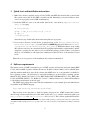
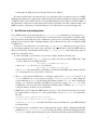
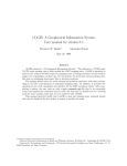
Figure 1: ETOPO5, NUVEL1 plate boundaries and PDE hypocenter distribution as of example1.ps, resolution reduced. Data from DeMets et al. (1990); NOAA (1988); USGS/NEIC (1998).
be done (in addition to the introduction in the GMT manual) and give the experienced user a fast tool to
get to a start script for more complicated applications. This file is called $HOME/igmt_parameters.dat by
default. Addstufftothepscoastline lets the user add additional commands to the last pscoast command
of the script file without having to exit from iGMT and run the script independently. The file presented by
Showscripterrors contains the stderr output of the GMT commands invoked and should be helpful for
debugging. By default, GMT is “verbose”. GMTversion lets the user change between the old GMT version
3.0 and one of the newer versions, such as 3.4. The last item of this menu lets the user switch the GMT logo
on and off. By default, it is off since it would interfere with the colorbars.
7.6
Menu GMT help
This menu list is intended to provide fast access to the GMT man pages for reference. At the time of the
first call, a temporary file is created from the man command and afterwards displayed every time the user
selects the same command man page again. If the GMT man pages are not in the usual place where the man
command looks for them, uncomment the line
Finally, the two buttons on the right hand side of the menu bar do what they say.
8
Examples
The following examples were produced by running iGMT with the full data sets as described above. They
can be reproduced if the data is available locally by loading the parameters file given in the distribution.
Hypocentres from the NEIC dataset Figure 1 shows the map of example1.ps from the iGMT distribution, the whole Earth in the Mollweide projection. ETOPO5 in 60 arc minute resolution is the ground raster
15
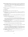
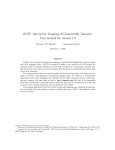
Figure 2: A part of the Carlsberg ridge in the Indian Ocean as of example2.ps, parameters can be loaded
from example2.dat. The original file has extremely high resolution and was quite big. The reduced image
shown here was shrunk to 81dpi using xv. Bathymetry data is from Smith and Sandwell (1997), plate
boundary from DeMets et al. (1990), scale is the same than in Fig. 1.
layer. All hypocentres of the USGS/NEIC dataset from 1973 – 1997 with magnitude greater than five and
NUVEL1 plate boundaries are superimposed. Load example1.dat to produce this plot. To reduce the size
of this documentation, the postscript file is not exactly that produced by iGMT but a converted GIF with
lower resolution.
Smith & Sandwell/GTOPO30 topography Figure 2 of example number two shows a part of the Indian
ocean and the Indian subcontinent. It was produced using the Smith & Sandwell/GTOPO30 dataset in
full resolution and has the pscoast shoreline data in high resolution superimposed. The original map has
fascinating detail that might be lost in this reproduction.
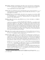
Sea-floor age of Müller et al. Example 3 as resp-resented by Fig. 3 and the files example3.ps and
example3.dat shows the North Atlantic region sea-floor age data coverage together with plate boundaries
(Stereographic projection).
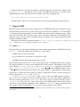
Gravity anomalies from Sandwell and Smith (1997) The last example (example4.*) of Fig. 4 shows
gravity anomalies in the Indian ocean. ATTENTION: This example is quite resource hungry and might
lead to problems on smaller machines if actually run with the original data set!
16
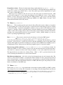
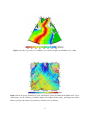
Figure 3: Sea-floor age version 1.3 of Müller et al. (1997b) and plates from DeMets et al. (1990).
Figure 4: Free-air gravity anomalies in a part of the Indian ocean from Sandwell and Smith (1997). Dominant features are the Carlsberg, Southwest Indian and Southeast Indian ridges, the Bengal fan and the
Ninety-east ridge. Resolution was restricted to 10 instead of 2 arc minutes.
17
9
Conclusion
The iGMT software package was programmed in a modular way. Every routine is commented, so it should
be fairly easy to modify the code and add extensions to the software. If you do so, that’s fine, but please
do not call it iGMT when you distribute it and make reference to the original software. Please keep in
mind that while GMT offers a large number of interesting and useful mapping options and iGMT tries to
make use of them, iGMT can’t be as flexible as GMT. In addition, it is pretty hard to test every single
combination of what-might-go-wrong-if. Hence, iGMT can be expected to fail to produce useful maps
under certain circumstances. Of course, the software is provided as is, no guarantee whatsoever is given and
no responsibility for possible damage is taken.
Hopefully, iGMT demonstrates what can be done nowadays that great geophysical data sets and mapping
software is available. If iGMT helps in making the research work of earth scientists easier, we are happy.
References
DeMets, C., Gordon, R. G., Argus, D. F., and Stein, S. (1990). Current plate motions. Geophys. J. Int.,
101:425–478.
Dunbar, P. K., Lockridge, P. A., and Whitewide, L. S. (1997).
Catalog of Significant Earthquakes 2150 B.C.–1991 A.D. Report SE-49. National Geophysical Data Center, Boulder, Colorado.
http://www.ngdc.noaa.gov/seg/hazard/sigintro.html.
Dziewoński, A. M. and Woodhouse, J. H. (1983). Studies of the seismic source using normal-mode theory.
In Kanamori, H. and Boschi, E., editors, Earthquakes: observation, theory, and interpretation: notes from
the International School of Physics “Enrico Fermi” (1982: Varenna, Italy), pages 45–137. North-Holland
Publ. Co., Amsterdam.
EDC (1996). Global 30 Arc Second Elevation Data Set. EROS Data Center, Sioux Falls, South Dakota.
Engdahl, E. R., van der Hilst, R. D., and Buland, R. (1998). Global teleseismic earthquake relocation with
improved travel times and procedures for depth determination. Bull. Seismol. Soc. Am., 88:722–743.
Giardini, D., Grünthal, G., Shedlock, K., and Zhang, P. (1999). The GSHAP Global Seismic Hazard Map.
Annali di Geofisica, 42:1225–1230.
Giardini, D., Grünthal, G., Shedlock, K., and Zhang, P. (2000). The GSHAP Global Seismic Hazard Map.
Technical report, ETH Zürich, http://seismo.ethz.ch/gshap/global/global.html.
Gilly, D. (1994). UNIX in a Nutshell. O’Reilly & Associates, Inc., Cambridge.
Gudmundsson, O. and Sambridge, M. (1998). A regionalized upper mantle (RUM) seismic model. J.
Geophys. Res., 103:7121–7136.
Laske, G. and Masters, G. (1997). A global digital map of sediment thickness. EOS, Trans. AGU, 78:F483.
Müller, B., Reinecker, J., and Fuchs, K. (2000). The 2000 release of the World Stress Map. Online at
www.world-stress-map.org, cf. Zoback (1992).
Müller, B., Wehrle, V., and Fuchs, K. (1997a). The 1997 release of the World Stress Map. http://wwwwsm.physik.uni-karlsruhe.de/pub/Rel97/wsm97.html.
18
Müller, D., Roest,
Digital isochrons
W. R.,
of the
Royer, J.-Y., Gahagan,
world’s ocean floor.
L. M., and Sclater,
J. Geophys. Res.,
http://Omphacite.es.su.oz.au/StaffProfiles/dietmar/Agegrid/agegrid.html.
J. G. (1997b).
102:3211–3214.
Nakiboglu, S. M. (1982). Hydrostatic theory of the Earth and its mechanical implications. Phys. Earth
Planet. Inter., 28:302–311.
NOAA (1988). Data Announcement 88-MGG-02, Digital relief of the Surface of the Earth. National
Geophysical Data Center, Boulder, Colorado. http://www.ngdc.noaa.gov.
Ousterhout, J. K. (1993). TCL and the TK Toolkit. Addison-Wesley, Reading, MA.
Rapp, R. H., Wang, Y. M., and Pavlis, N. (1991). The Ohio State 1991 geopotential and sea surface topography harmonic coefficient models. Rep. 410, Dept. of Geod. Sci. and Surv., Ohio State University,
Columbus, Ohio.
Rapp, R. H., Zhang, C., and Yi, Y. (1996). Analysis of dynamic ocean topography using topex data and
orthonormal functions. J. Geophys. Res., 101:22583–22598.
Reinecker, J., Heidbach, O., and Müller, B. (2003). The 2003 release of the World Stress Map. (Online at
www.world-stress-map.org).
Sandwell, D. T. and Smith, W. H. F. (1997). Marine gravity anomaly from Geosat and ERS-1 satellite
altimetry. J. Geophys. Res., 102:10039–10050.
Simkin, T. and Siebert, L. (1994). Volcanoes of the World. Geoscience Press, Tucson, Arizona, 2nd edition.
http://www.volcano.si.edu/gvp/volcdata/index.htm.
Smith, W. H. F. and Sandwell, D. T. (1997). Global seafloor topography from satellite altimetry and ship
depth soundings. Science, 277:195–196. http://topex.ucsd.edu/marine topo/mar topo.html.
Steinberger, B. (2000). Plumes in a convecting mantle: Models and observations for individual hotspots. J.
Geophys. Res., 105:11127–11152.
USGS/NEIC (1998). National Earthquake Information Center, World Data Center A for Seismology.
Global Earthquake Search. United States Geological Survey, National Earthquake Information Center,
http://wwwneic.cr.usgs.gov/neis/epic/epic global.html.
Wessel, P. and Smith, W. H. F. (1991). Free software helps map and display data. EOS Trans. AGU,
72:445–446.
Wessel, P. and Smith, W. H. F. (1995). New version of the Generic Mapping Tools released. EOS Trans.
AGU, 76:329.
Wessel, P. and Smith, W. H. F. (1998). New, improved version of the Generic Mapping Tools released. EOS
Trans. AGU, 79:579.
Zoback, M. L. (1992). First- and second-order patterns of stress in the lithosphere: The World Stress Map
project. J. Geophys. Res., 97:11703–11728.
19
Appendix
A
Technical details
A.1
Organization of the iGMT software
After unpacking the igmt_v1.2.tar file the directory should look something like this
> ls -F
COPYING
COPYRIGHT
INSTALL.TXT
NOTES.TXT
README.TXT
colminmax.awk
colormaps/
configure_script*
example1.dat
example2.dat
example3.dat
example4.dat
formatcpt.awk
igmt*
igmt.tcl
igmt_configure.tcl
igmt_datasets.tcl
igmt_def.gif
igmt_gmtdefaults_3.0
igmt_gmtdefaults_3.1
igmt_gmtdefaults_3.2
igmt_gmtdefaults_3.3
igmt_gmtdefaults_3.4
igmt_helper_checkfile*
igmt_helper_create_ci_file*
igmt_helper_create_man_page*
igmt_helper_handle_gmtdefaults*
igmt_helper_rmtmp_silent*
igmt_init.tcl
igmt_iomisc.tcl
igmt_menus.tcl
igmt_parameters.tcl
igmt_plotting.tcl
img2grd*
sortwsm.awk
where the colormaps directory contains the color tables for GMT.
> ls
bathymetry.cpt
col.00.cpt
col.01.cpt
col.02.cpt
col.03.cpt
col.04.cpt
col.05.cpt
col.06.cpt
col.07.cpt
col.08.cpt
col.09.cpt
col.10.cpt
col.11.cpt
col.12.cpt
col.13.cpt
col.14.cpt
col.15.cpt
col.16.cpt
col.17.cpt
col.18.cpt
col.19.cpt
col.20.cpt
col.21.cpt
col.22.cpt
col.23.cpt
col.24.cpt
col.25.cpt
col.26.cpt
col.27.cpt
col.28.cpt
col.29.cpt
col.30.cpt
col.31.cpt
col.32.cpt
col.33.cpt
col.34.cpt
col.35.cpt
col.36.cpt
col.37.cpt
col.th.1.cpt
colgeoid.cpt
geoid.cpt
geoid2.cpt
geoid3.cpt
geoid5.cpt
gravity.cpt
seafloor_age.cpt
seafloor_age2.cpt
sediment.2.cpt
sediment.cpt
tomo.cpt
tomo2.cpt*
topo.bw.cpt
topo.cpt
topo1.cpt
topo2.cpt
topo3.cpt
topo4.cpt
The files in this distribution can be classified as follows:
Copyright: COPYING and COPYRIGHT deal with legal issues. iGMT is distributed under the GNU public
license but should be used in accordance with the Student Pugwash Pledge, see the file COPYING.
configure script: This short script is supposed to take over the installation process as described in sec. 5.
img2grd: Script from the GMT distribution that is supposed to be a patch when img2latlongrd is not
available, included starting from GMT 3.3.6.
The igmt file: A bash script that is used to check if the environment variable $igmt_root and wish is
available at the places iGMT is looking. If all is fine, wish is invoked with igmt.tcl. igmt_def.gif is the
start-up screen.
20
Tcl files: All files with the tcl extension contain the tcl code that runs iGMT. igmt.tcl is the main file, it
contains source commands and builds up some frames. igmt configure.tcl has all global variables and
the default settings for plotting whereas igmt_init.tcl handles the startup sequence. The file igmt_menu.
tcl holds the definition for the main menu line and the procedures found in igmt_datasets.tcl, igmt_
parameters.tcl and igmt_plotting.tcl correspond roughly to all possible actions in the individual pulldown menus. Finally, igmt_iomisc.tcl contains most of the input/output routines and some additional tcl
procedures.
All of these files should be fairly well commented so that we won’t go into any detail here.
igmt helper files These contain small bash scripts that are called by iGMT’ tcl routines and handle
more operating system based processes. Most of them could be integrated into the main tcl code but it
seemed more transparent for possible porting to other operating systems to keep them external.
example.dat and .ps: The dat files contain the parameter dump that was created with iGMT after the
examples presented in section 8 were produced. The postscript files are packed with gzip and correspond
to the shrinked figures in this manual and are not identical to the real postscript files produced (they were
too big to be included in the distribution).
Documentation and data The file manual.ps is the manual you are reading as a postscript file. nuvel.
yx is the modified plate boundary polygon file after DeMets et al. (1990), 01_02-98.cmt contains the
Harvard CMT double couple fault plane solution for the first 60 days of 1998 as an example, vocanoes.dat
the volcano locations after Simkin and Siebert (1994), allslabs_rum.gmt the slab seismicity contours of
Gudmundsson and Sambridge (1998) and hotspots.dat the hotspot list of Steinberger (2000).
Colormaps: The colormaps directory contains the colormaps that are used by iGMT to map the default
datasets. col.00.cpt through col.35.cpt are generic colormaps which span the data range from −1 . . . 1.
If you want to convert these colormaps to suit your data, use an awk script like colminmax.awk which
comes with the iGMT distribution.
# script to convert the data range of colorscale files for GMT
# by rescaling
BEGIN{
if(min==0)min=-1.;
if(max==0)max=1.;
mean=(max+min)/2.;
range=(max-min)/2.;
printevery=50;
}
{
if(NR<256){
if(printevery - NR > 0)
print($1*range+mean,$2,$3,$4,$5*range+mean,$6,$7,$8,$9);
else {
print($1*range+mean,$2,$3,$4,$5*range+mean,$6,$7,$8,$9,"L");
printevery=NR+printevery;
}
}
else
21
print($0);
}
If your data sets contains values between −2 and 3, say, and you would like to use the rainbow colored
colorscale col.13.cpt, use
awk-f$igmt_root/colminmax.awkmin=-2max=3\ldots\\$igmt_root/colormaps/col.13.cpt>
new_colormap.cpt.
Here, “. . . ” means that the above should be in one line.
Also, you might want to use the grd2cpt function of GMT that can be accessed over createcolormap
menu item.
B
Modifying iGMT
iGMT may be freely modified and distributed as long as modified versions are not called iGMT. There are
plenty of easy possible future enhancements one could think of, for instance interactive design of colormaps,
support of more complicated user data sets and multiple layers of raster data. When this extensions become
available, they will be included in future versions. Some common modification (as opposed to extension or
enhancement) tasks are described below:
Using other path names for the data sets. All pathnames to data locations are assigned in igmt_configure.
tcl. All raster data sets have two variables assigned to them: raster data(i) and raster_colormap(i),
they refer to the location of the raster data set number i and the location of the default colormap, respectively. Simply add a line like setraster_data(3)"/home/user/gtopo30/topo_6.2.img" to your
igmt_siteconfig.tcl file, if your GTOPO30 dataset (number 3 internally) is in /home/user/gtopo30/.
The equivalent variables for polygon data are called poly_data(i), and it is simplest to search for the
appropriated variable names in igmt configure.tcl.
Including new data sets. You will have to do these things: (to be expanded)
1. Add the data location and its parameters to the igmt_configure.tcl file.
This should be easier now with version 1.2 since we have replaced most global variables for raster and
polygon data issues with arrays, such that you can simply add one more entry at the back. Right now,
raster data sets are reserved from 1 to 11, with the limit being set to (variable: nr_of_raster_data)
20 raster data sets in total. Polygon data sets are restricted to 25, and right now all sets up to 20 are
filled. Read through igmt configure.tcl to see how the default data sets are implemented here.
Parameters for raster data are: location of data file, default colormap, geographical limits (East, West,
South, and North boundaries), integer boundaries only (on/off), the maximum resolution (in arc minutes), and resampling at other than default grid spacing (on/off). For polygon data: location of data,
symbol size, symbol color, . . .
2. Add the data selection choice to the Datasets menus. This is done in igmt_menues.tcl and igmt_
datasets.tcl.
22
3. Add the data plotting routine to igmt_plotting.tcl, taking the old datasets as an example. Make
use of the predefined standard procedures for raster data.
23