Download User Manual for Cascade Version 4.0

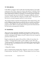
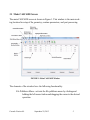
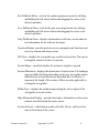
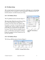
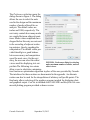
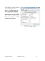
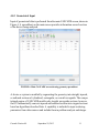
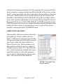
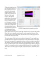
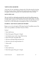
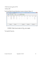
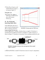
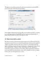
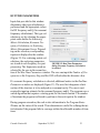
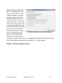
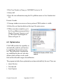
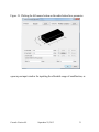
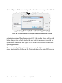
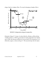
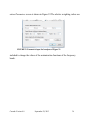
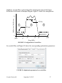
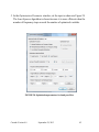
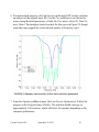
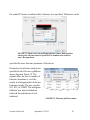
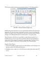
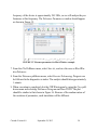
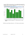
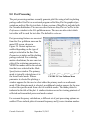
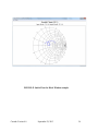
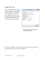
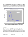
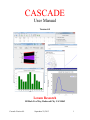
CASCADE
User Manual
Version 4.0
Lexam Research
10 Black Fox Way, Redwood City CA 94062
Cascade Version 4.0
September 29, 2013
1
Table of Contents
1.0 Introduction ..........................................................................................3
2.0 Installation ............................................................................................3
3.0 Program Execution ...............................................................................5
4.0 Problem Setup ......................................................................................9
5.0 Run Setup and Execution ...................................................................22
6.0 Optimization .......................................................................................29
7.0 Tolerance Analysis .............................................................................45
8.0 Post Processing...................................................................................52
9.0 Troubleshooting..................................................................................58
10.0 Appendix A Examples
11.0 Appendix B: Engine and Auxilliary Codes
12.0 Appendix C: External Scattering Matrix File
Lexam Research
10 Black Fox Way
Redwood City CA 94062
(650) 488-8323
Email: [email protected]
Copyright 1999-2003
Cascade Version 4.0
September 29, 2013
2
1.0 Introduction
CASCADE is a computer code for rapid and user-friendly analysis of waveguide
components such as filters, microwave cavities, and windows. It calculates scattering parameters (transmission/reflection coefficients) for general waveguide structures composed from cylindrical, rectangular, or coaxial waveguides. Transitions
between waveguide types are also allowed. The program includes the dielectric
properties of ceramics and finite conductivity of metal surfaces. The program will
also solve for resonant frequencies and Qs of cavity structures.
The program includes an optimizer that dramatically reduces design time by selectively modifying design parameters specified by the user to achieve specified performance. The program can also input scattering matrices from other computer
programs (such as HFSS) or measured data and incorporate that information into
the total system scattering matrix calculation.
2.0 Installation
There are two steps required the install the Cascade software. The first is downloading the Cascade distribution from the link provided to you by email. The second step is obtaining the MAC address of your PC which is to be sent to Lexam for
generation of the license file.
Begin by extracting the contents of the zip file to a folder (of your choice, for
example “C:\Program Files\Cascade\”) on the computer. Create a link to the
"Cascade_gui.exe" file located in the folder containing the binary executable files
and move the link to your desktop for easy access to the program. Then complete
the following steps:
1) Obtain MAC address
Open a command prompt window (Start->Programs->Accessories->Command
Prompt) and type “ipconfig /all”. Find the “Ethernet adapter Local Area Connec-
Cascade Version 4.0
September 29, 2013
3
tion:” section of the output from the command. Under this section there is an entry
for “Physical Address” which has a 12 digit value. This is the MAC address value
to be sent to Lexam for generation of your license file.
2) License File Installation
After receipt of the license file for your software from Lexam, copy the file to the
folder where the Cascade binary executable files were stored. There is no particular name required for the folder.
3) Define executable locations
The various components that provide the functionality for the Cascade GUI
(Cascade_GUI.exe) such as the main computational engine (Cascade.exe) and S
parameter postprocessor (scattout.exe) are designed to run directly from the command line for custom usage by the user, for example a Matlab script file. The
command line arguments and input/output file format are described in the appendendices. The first time the Cascade GUI is called the locations of the various Cascade executable must be defined for execution by the GUI. This is performed by
selection of Settings->Preferences from the pulldown menu. In the Paths block
click on the Executable paths dialog browse button and select the folder where the
Cascade executables are stored. If all the required executables are there the list of
executables names will be followed by the full path name highlighted in green
(Figure 4).
3.0 Program Execution
Start the program by executing the cascade_GUI.exe in your Cascade binary executable files directory or shortcut link. The program opens up windows, as shown
in Figure 1.
Cascade Version 4.0
September 29, 2013
4
3.1 Main CASCADE Screen
The main CASCADE screen is shown in Figure 1. This window is the main working location for setup of the geometry, runtime parameters, and post processing.
FIGURE 1. Main CASCADE Window
The elements of the window have the following functionality:
File Pulldown Menu - activate the file pulldown menu by clicking and
holding the left mouse button and dragging the cursor to the desired
operation.
Cascade Version 4.0
September 29, 2013
5
Run Pulldown Menu - activate the runtime parameters menu by clicking
and holding the left mouse button and dragging the cursor to the
desired operation.
View Pulldown Menu - activate the post processing features by clicking
and holding the left mouse button and dragging the cursor to the
desired operation.
Help Pulldown Menu - displays information on software version and contact information for the software developer.
Function Buttons- provides quick access to commonly used functions and
access to runtime and setup screens.
WG Type - displays the waveguide type used for each section. This can be
rectangular, coaxial, circular, or external.
Section Shape - specified whether the section is straight or tapered
Section Dimension - displays the dimensions of each section. The headings
represent different things depending on the type waveguide and are
defined in the section edit screens described later. In all cases, L
represents the length of the section. Offsets are only applicable to
rectangular waveguides.
Media Type - displays the medium representing the active region of the
waveguide or circuit section.
Help Information Display - provides descriptive information on the screen
element located beneath the mouse cursor.
Section Selector - radial buttons used by the Edit, Delete, and Insert buttons at the bottom of the screen.
Cascade Version 4.0
September 29, 2013
6
Add Section Button - activates section selection browse window for adding
additional sections to the bottom of the spreadsheet (right end of the
geometry).
Edit Section Button - activates the section input screen for the section indicated by the Section Selector radial buttons. This allows the user to
modify the information for a particular section.
Delete Section Button - deletes the section indicated by the Section Selector radial buttons. Verification is required by the user before the
function is performed.
Insert Section Button - inserts a section before the section indicated by the
Section Selector radial buttons. This activates the Section Type
Selection window.
Draw Geometry - draws a side and top view image of rectangular geometries and a side view of cylindrical and circular geometries. A centerline is inserted for coaxial and circular sections.
Cascade Version 4.0
September 29, 2013
7
4.0 Problem Setup
This section describes the elements required for initializing a case and inputting
the geometry of the waveguide or circuit components. Following sections will
describe analysis execution and post processing.
4.0.1 File Pulldown Menu
The File pulldown menu is shown in Figure 2.
The menu items allow the user to Open existing
files, clear the spreadsheet to begin a New
geometry, Save the current case with the same
case name, or use Save As to save the case under
a different name. Browse windows with appropriate filters are activated for user input where
necessary. The Exit function terminates the program. A verification screen appears if information in the program has been changed since the
last Save operation.
FIGURE 2. File Pulldown
Menu
4.0.2 File Pulldown Menu
The Settings pulldown menu is shown in Figure 3.
FIGURE 3. Settings Pulldown Menu
Cascade Version 4.0
September 29, 2013
8
The Preferences selection opens the
dialog shown in Figure 4. The dialog
allows the user to select the units
used in the design and the maximum
number of modes allowed for an
analysis. The default values are
inches and 1000, respectively. The
next entry controls how many modes
are coupled between adjacent transitions. Modes whose amplitude have
dropped below this entry are not used
in the cascading of adjacent scattering matrices, thereby speeding the
computation. The default values provided should give a good balance
between accuracy and computation
speed for most cases. On the next
entry, the user can select the editor/
FIGURE 4. Preferences dialog for selecting
viewer used for displaying text outunits, maximum number of modes, and text
editor/viewer.
put data The following two entries
allow a user to substitute a minimization function or optimization algorithm in place of the ones provided by Cascade.
The interfaces for those routines are documented in the appendix. An alternate
routine can also be used for the interpolation of arbitrary wall profile points. The
final entry allows selection of the graphics program invoked for displaying plots
and graphical output. CasPlot is included with CASCADE and EasyPlot is a commercial plotting program provided as demo version.
Cascade Version 4.0
September 29, 2013
9
The Configure Toolbars selection
opens the dialog shown in
Figure 5. The dialog allows the
user to set the most commonly
accessed functions in the pulldown menus as one-click options.
It is particularly useful for setting
the most commonly accessed View
functions for easy access.
FIGURE 5. Configure Toolbars
Cascade Version 4.0
September 29, 2013
10
4.0.3 Geometrical Input
Input of geometrical data is performed from the main CASCADE screen, shown in
Figure 6. A spreadsheet on the main screen provides information on each section
of the device being analyzed.
FIGURE 6. Main CASCADE screen showing geometry spreadsheet.
A device or system is modeled by segmenting the geometry into straight, tapered,
or radiused sections of cylindrical, rectangular, or coaxial waveguide. The computational engine of CASCADE models only straight waveguide sections; however,
the GUI automatically converts tapered and radiused sections into stepped sections
based on algorithms described later. A capability is included to input scattering
parameters from other sources and include them in problem analysis and design.
Cascade Version 4.0
September 29, 2013
11
Geometrical information is added in the GUI beginning at the extreme left of the
device or structure, and new sections are added to the right of the previous section.
As new sections are added, a new line is appended to the spreadsheet on the main
GUI screen. The ID number of each section is shown in the first column of the
spreadsheet. The following columns indicate the waveguide type, shape, dimensions, relative position, and medium of each section. Buttons along the bottom of
the screen allow the user to ADD, EDIT, DELETE, or INSERT waveguide sections.
INSERT locations and sections to be edited or deleted are identified using the radio
buttons in the first column. At anytime, the user can see a plot of the sections
entered by selecting the DRAW GEOMETRY button.
ADDING NEW SECTIONS
Selection of the Add Section button activates the
waveguide type selection window shown in
Figure 7. Selection of a waveguide type activates
the appropriate input window for that waveguide
type. Figure 8 shows the input window for a
Tapered Coax Section. The last geometry type
shown in the Available Geometries: window is
External Scattering Matrix File. This allows the
user to input S-parameters obtained from experimental measurement or from other programs,
such as Ansoft’s High Frequency Structure Simulator. This feature will be described later.
FIGURE 7. Waveguide Type
selection window
Cascade Version 4.0
September 29, 2013
12
All geometry input screens
are functionally similar. At
the top of each screen is a
section for selecting the
medium inside the waveguide section and the conductivity of the metal
surfaces. The default
media value is Vacuum and
the default conductivity is
Perfect Conductor; however, alternative materials
can be selected by clicking
on the Specify button and
selecting materials using
the radio buttons. Selection
FIGURE 8. Input window for tapered coax section
of a listed material automatically loads the appropriate values into the text boxes to the right. Selection of the Custom radio button
allows the user to manually enter alternative values using the keyboard. After
selection of the Custom radio button, left click the mouse in the appropriate text
box and enter the desired value.
The center region of the input screen contains a diagram of the waveguide type
with all dimensions labeled with capital letters. These dimensions are described
below and correspond to the appropriate columns in the main window spreadsheet.
The TAB key will sequentially advance the user through the text boxes. Alternatively, specific text boxes can be activated using the left mouse button. The input
window for rectangular sections contains additional inputs for waveguide offsets.
These can be used for stepped waveguide, asymmetrical irises, and similar structures.
Cascade Version 4.0
September 29, 2013
13
Each parameter contains a radio button for selecting this parameter for optimization. Selection of the radio button activates a window for input of allowed ranges
of the parameter. Use of the optimizer will be described below.
When the OK button is selected, the window is closed and the information transferred to the main window spreadsheet. The OK button will not function if any text
box contains incomplete or illegal data. In this situation, the user should carefully
check that all appropriate inputs are entered correctly.
EDIT SECTION
Use the mouse to select the radio button corresponding to the section to be modified. Clicking the left mouse button on the Edit Section button will result in display of the input window for that section with current values for all parameters.
Use the left mouse button and keyboard to modify the entries. Selection of the OK
button will close the window and update the spreadsheet.
INSERTING SECTIONS
To insert a section, use the mouse to activate the radio button of the section in the
spreadsheet that will follow the new section. The waveguide type selection window will appear, and the user selects the appropriate type. This will activate the
input window for the new section, and the user proceeds as described above.
Selection of the OK button will result in insertion of the new section in the spreadsheet and renumbering of the following sections.
DELETING SECTIONS
To delete a section, use the left mouse button to activate the appropriate radio button in the first column of the spreadsheet. Selection of the Delete Section button
will activate a confirmation window for the user to verify the delete request. Following verification, the information will be removed from the spreadsheet, and the
following sections will be renumbered.
Cascade Version 4.0
September 29, 2013
14
VIEWING THE GEOMETRY
At any time, the user can display a schematic plot of the data entered by selecting
the Draw Geometry button. Cylindrical and coaxial sections are delineated from
rectangular sections by the presence of a centerline drawn in those sections.
SAVING THE CASE
The user should save information periodically using the File pulldown menu on
the main screen or the Save function button shown on the Main window. The name
provided will be used for storage of all subsequent input and output files generated
by the GUI or CASCADE engine with appropriate suffixes for identification.
EXAMPLE 1. RECTANGULAR BLOCK WINDOW
Begin a new case by selecting the NEW option from the File pulldown menu if the
main screen spreadsheet is not blank. Proceed as follows:
Section 1
1. Select Add Section
2. Select Rectangular Waveguide - Straight
3. Left click the mouse in the A-Input Width text box
4. Enter 0.28 for the waveguide width
5. Tab twice to B-Input Height and enter 0.14
6. Tab twice to Section Length and enter 1.0
7. Click on OK
Section 2
8. Select Add Section
9. Select Rectangular Waveguide - Straight
Cascade Version 4.0
September 29, 2013
15
10.Select the Rf Medium: Specify button. Select the Custom radio button and, in
the text boxes, enter 0.9323 as the dielectric constant and 0.0 for the loss tangent (The loss tangent is not currently used by the program). Click OK to close
the window.
11.Left click the mouse in the A-Input Width text box
12.Enter 0.274 for the waveguide width. The reduced dimension provides for
braze material between the ceramic and the waveguide wall.
13.Tab twice to B-Input Height and enter 0.1345
14.Tab twice to Section Length and enter 0.0707
15.Click on OK
Section 3
16.Select Add Section
17.Select Rectangular Waveguide - Straight
18.Left click the mouse in the A-Input Width text box
19.Enter 0.28 for the waveguide width
20.Tab twice to B-Input Height and enter 0.14
21.Tab to Section Length and enter 1.0
22.Click on OK
Cascade Version 4.0
September 29, 2013
16
Verify that main Cascade window is the same as shown in Figure 9.
FIGURE 9. Main Cascade window for BlockWndw example
Viewing the Geometry
23.Select Draw Geometry
and confirm that the
geometry is as shown in
Figure 10. There are two
geometry plots shown,
one for the top (waveguide width,dimension A
in the table) and the side
view which is the waveguide height.
Saving the Case
FIGURE 10. Top view (waveguide width) for
Rectangular Block Window.
Cascade Version 4.0
September 29, 2013
17
24.From the File pulldown, select Save As and save the case with the name BlockWndw.
Example 2: TE01 Gyrotron Cavity
Begin a new case by clicking the NEW button at the top of the CASCADE main
window if the main screen spreadsheet is not blank. Proceed as follows:
Section 1
1. Select Add Section
2. Select Circular Waveguide - Straight, then OK
3. Enter 0.122 in the A- Input Diameter text box
4. Tab twice to Section Length and enter 0.2
5. Select OK
Section 2
6. Select Add Section
7. Select Circular Waveguide - Straight, then OK
8. In the A- Input Diameter text box, enter 0.1555
9. Tab twice to Section Length and enter 0.3425
10.Select OK
Section 3
11.Select Add Section
12.Select Circular Waveguide - Tapered, then OK
13.In the A- Input Diameter text box, enter 0.178
14.In the B - Output Diameter text box, enter 0.30
Cascade Version 4.0
September 29, 2013
18
15.Set Section Length to 0.754
16.Select OK
Verify that Main Screen information is same as shown in Figure 11.
FIGURE 11. Main Cascade window for TE01 cavity example
Viewing the Geometry
Cascade Version 4.0
September 29, 2013
19
17.Select Draw Geometry and
confirm that the geometry is
as shown in Figure 12.
Saving the case
18.From the File pulldown,
select Save As and save the
case with the name
TE01cavity.
4.1 Use of External
Scattering Matrix Files
CASCADE allows the user to
input external scattering matrix
FIGURE 12. Geometry plot for TE01 Cavity
files as sections in the device
being modeled. This has two
obvious applications. Consider a situation where a complex 3-D structure is
mounted between standard 2-D coaxial, rectangular or circular structures, as
shown in Figure 13. Typically, it is necessary to use an advance mesh code, such
3-D Structure
(Black Box)
Input
Output
Matching Elements
FIGURE 13. Example of using external scattering matrix files to model
complex structures
as HFSS and MAFIA, to model 3-D structures; however it may be computation-
Cascade Version 4.0
September 29, 2013
20
ally impractical or inconvenient to model the entire device or system with these
codes. Using the facility in CASCADE, the user can model the complex structure
in the mesh code and save the scattering parameters to an disk file. The user can
then read in this file and treat this information as a “Black Box” section of the
device whose scattering parameters are now known. The remaining sections can
be added using the Add facility in Cascade and the entire system modeled as a single entity. The Optimizer can be invoked to modify the standard elements in the
geometry to obtain the desired performance characteristics of the entire device or
system. In Appendix A is an example where matching elements are used to match
a TE01 circular to TE10 rectangular mode converter to standard rectangular and
circular waveguide.
The second obvious application is in designing matching elements for hardware
whose scattering parameters have been experimentally measured. One could, for
example, measure the complex reflection coefficient at the input of a helix traveling wave circuit. The measured scattering matrix data would be used as the last
section in a CASCADE model to design matching elements, including the input
window. In this way, the output waveguide and window would be precisely
designed to provide the optimal match to the input helix.
The user selects External Scattering File at the bottom of the Available Geometries window shown in Figure 7. This will result in the appearance of the External
Scattering Matrix File window shown in Figure 14 Note that it is necessary to
specify the input and output geometry type for the device so that the imported scattering matrix is normalized to the appropriate impedance. From this point on, the
Cascade Version 4.0
September 29, 2013
21
file appears as any other section in the geometry, except that it is labeled differently on the main CASCADE GUI spreadsheet.
FIGURE 14. Input window for inputting external scattering matrix file
Two examples using external scattering files are provided in Appendix A. The first
uses scattering parameters from HFSS, and the second uses measured data to
match an input window to a helix traveling wave tube.
5.0 Run Setup and Execution
Execution control is performed using input windows accessed from the Run pulldown on the main GUI screen or the Function Buttons at the top of the main GUI
window. Input data determines what type of analysis is performed (Scattering
matrix calculation, resonant frequency calculation, or determinant sweep to check
for resonant modes). Frequency values, modal input, and other parameters
required for program execution are entered here. Where appropriate, default values are provided. For most situations, these will be adequate, but the user always
has the option of selecting alternative values.
Cascade Version 4.0
September 29, 2013
22
RUNTIME PARAMETERS
Input data provided in this window
determines what type calculation is
performed and the appropriate values
for RF frequency and Q (for resonant
frequency calculations). The type calculation is set by selecting the appropriate radio button for Scattering
Matrix Calculation, Resonant Frequency Calculation, or Scattering
Matrix Determinant Sweep. Depending on the selection, corresponding
inputs are displayed in the window
(Figure 15). For scattering matrix calculations, the scattering parameters
FIGURE 15. Run Time Parameters
are stored at each frequency for post
dialog. Resonant Frequency Calculation
processing. The frequencies used are
is selected.
selected by the user in the second section of the Run Time Parameters window. The user can input the Number of Frequencies or the Frequency Step, and the GUI will calculate the alternate value.
If a resonant frequency calculation is selected, additional entries in the RunTime
Parameters window are displayed (Figure 15). The user first designates which
section of the structure is to be analyzed as a resonant cavity. The user is next
required to input an estimate for the resonant frequency and Q. The program uses a
search algorithm that requires a starting point for the search routine. The number
of iterations the program is allowed to perform is the next input in the window.
During program execution, the code writes information to the Program Status
Window on the status of the search. This information is useful for refining the initial estimate if the program fails to converge within the allowable number of iterations.
Cascade Version 4.0
September 29, 2013
23
Following successful execution, the program can write the field information to a
file for input to other codes. The inputs at the bottom of the Run Time Parameters
window allow the user to select this option and specify the axial extent of the field
information written to file. The format of the output file is described in the Appendix.
The Scattering Matrix Determinant Sweep allows the user to search the geometry
for trapped modes and ghost modes. The family of modes used in the search are
described in the Mode Parameters section below. For the determinant sweep, the
user specifies the start and stop frequencies and the frequency step. The user also
specifies a Q value, which has a slight impact on the resolution of the search.
Mode Parameters
Input for the mode parameters is done from the dialog window selected by the
Run->Mode Parameters pull down menu or the This window (Figure 16) provides information on what modes are to be used during program execution. The
first input (Use modes up to X times cutoff) sets the number of modes to be used in
the scattering matrix calculations. The number of modes used in each section is
determined by selecting all modes up to those whose cutoff frequency is X times
the upper analysis frequency. The total computational time increases quadratically
with this input; however, failure to use a sufficient number of modes may result in
an inaccurate solution. A simple technique for determining the appropriate value
is to incrementally increase the input value until the simulation results converge.
The number of modes required depends on the dimensions of the geometry and the
frequency. Waveguide geometries with large reactive components (such as irises)
can require large numbers of modes. The filter example described in the optimization section below requires use of modes with cutoff frequency up to 80 times the
upper analysis frequency for accurate analysis.
The middle section of the window specifies the azimuthal mode number when the
entire geometry consists of only cylindrical or coaxial sections. If the azimuthal
mode number is zero, the user must further specify if TE or TM modes are to be
used.
Cascade Version 4.0
September 29, 2013
24
If the geometry consists of a
mix of rectangular and cylindrical sections, there are four
orthogonal mode sets which
can be selected. The default
(Standard Mode Set) selects
usage of a mode set with symmetry of the TE10 mode in the
rectangular guide and the TE11
in the circular guide. The alternate mode sets are typically
used in determinant sweeps to
FIGURE 16. Input screen for Mode Parameters
check for trapped or ghost
modes. To be complete, the
determinant sweep analysis
should be performed with all sets. A complete description of the mode sets used
for the four options is described in Appendix C (Cascade Engine).
Number of Steps in Tapered Sections
Cascade Version 4.0
September 29, 2013
25
Recall that CASCADE analyzes
systems by calculating the coupling
coefficients between geometries of
constant radial dimensions (or x,y
dimensions in rectangular geometries). Tapered and radiused sections
are analyzed by breaking them into a
series of steps. The GUI performs
this function automatically depending on the wavelength of the stop
frequency entered in the Run Time
Parameters window and the slope of
tapers. The user can override the
default values by specifying a fixed
number of steps for all tapers/radii
or by changing the algorithm scale
factor (Figure 17). Note that doubling the algorithm scale factor will
FIGURE 17. Input window for setting
approximately double the computanumber of steps in tapers
tion time. Convergence of the
results should be checked by
increasing the scale factor to ensure adequate modeling of the geometry with steps.
Initiating Program Execution
Analysis of the system is initiated by selecting Execute CASCADE from the Run
pulldown menu or clicking the Execute function button at the top of the main
screen. All diagnostic and status messages from the CASCADE compute engine
are written to the Program Status Window first opened by the start-up batch file. It
is strongly recommended that the windows on the computer screen be arranged so
that the lower portion of this window is visible.
Cascade Version 4.0
September 29, 2013
26
At the completion of execution a diagnostic information window appears if a problem occurred.
Generate Input Data Set Only
The final option in the Run pulldown menu allows the user to generate only the
input file for the CASCADE engine without initiating program execution. This is a
ASCII file with an extension of .cas. Advanced users can directly modify this file
with a text editor and manually execute the CASCADE engine from the MSDOS
prompt. The format of this file is included in the Appendix.
EXAMPLE: BLOCK WINDOW
From the File pulldown menu or the Open button on the main screen, open the
previously saved file called BlockWndw.
Run Time Parameters
1. Select Run Time Parameters at the top of the main GUI screen
2. Select the Scattering Matrix Calculation radio button (default)
3. For start frequency, enter 27.0
4. For stop frequency, enter 30.0
5. For Number of Frequencies, enter 101. Hit the return key and note that the Frequency Step size is automatically calculated and entered in the next text box.
6. Select OK
Mode Specification
7. Verify that the number of modes are 2 times cutoff. The mode set is automatically selected and requires no further input.
Cascade Version 4.0
September 29, 2013
27
Number of Steps in Tapered Sections
8. Since there are no tapers in this example, no input is necessary.
Execute Cascade
9. Arrange windows on screen so lower portion of DOS window is visible
10.Select Execute Cascade
EXAMPLE: TE01 CAVITY
From the File pulldown menu on the main screen, open the previously saved file
called TE01 cavity.
1. From the Run pulldown menu, select Run Time Parameters
2. Select Resonant Frequency Calculation
3. In the third section of the window, enter 2 as the section to analyze for resonance
4. Enter 94.0 as the Resonant Frequency Estimate
5. Enter 200 as the Q Estimate
6. For Request Mode Dump, select No.
7. Select OK
Mode Specification
8. Change the number of modes above cutoff to 3
9. Azimuthal Mode Number should be 0
10.TE modes should be selected
Number of Steps in Tapered Sections
11.Select to Over-Ride With User Specification
Cascade Version 4.0
September 29, 2013
28
12.Set Fixed Number of Steps per TAPERED Section to 30
13.Select OK
14.Save the case information using the File pulldown menu or Save function button.
Execute Cascade
15.Arrange windows on screen so lower portion of DOS window is visible
16.Select Execute function button at the top of the main screen.
17.When execution completes, go to
the View pulldown menu and select
Display Resonant Frequency and
Q. The results should appear as
shown in Figure 18.
6.0 Optimization
CASCADE includes the capability to
automatically optimize performance
by modifying dimensional parameters. The performance requirements
FIGURE 18. Results of TE01 Cavity
are established by the user who also
analysis
defines which surfaces can be modified and the allowable ranges of modification.
The program includes three optimization routines selectable by the user. These are:
• Quasi-Newton
• Non-Smooth
• Least Squares
Cascade Version 4.0
September 29, 2013
29
Alternative user-provided optimization routines can be specified in the Preferences option in the File pulldown menu. The format for these routines is specified
in the Appendix.
There are also three optimization functions.
• Minimize Reflection over Frequency Range - this is useful for matching waveguide components and windows so that the reflection is minimized over a frequency range specified by the user.
• Minimize/Maximize Reflection over Frequency Range - this is useful for band
pass and notch filters and designing broadband waveguide components and
windows.
• Over-Moded Waveguide Optimization - this is used for designing mode converters and overmoded waveguide tapers.
To use the optimizer, the user must define which dimensional parameters can be
varied and the allowable range for that variation. The input window of each section contains radio buttons for selecting parameters for optimization, as shown in
Cascade Version 4.0
September 29, 2013
30
Figure 19. Clicking the left mouse button on the radio button for a parameter
opens up an input window for inputting the allowable range of modification, as
Cascade Version 4.0
September 29, 2013
31
shown in Figure 19.The user must provide both a lower and an upper bound for the
FIGURE 19. Input window for specifying bounds of optimization variation.
optimization routine. When the user selects OK, the window closes and the radio
button changes to a red color to alert the user that this parameter is selected for
optimization. An asterisk will appear on the main GUI screen next to the corresponding parameter.
The user next selects the optimization parameters. The Optimization Parameters
screen is activated by clicking on the Optimize button on the main GUI screen or
Cascade Version 4.0
September 29, 2013
32
from the Optimize pulldown menu. The Optimization Parameters window is
shown in Figure 20.
FIGURE 20. Optimization Parameters input screen
The initial entry is for the maximum number of function evaluations (iterations) to
allow during optimization. The optimizer will continue to iterate on the solution
until it detects convergence or until the maximum number of function evaluations
is reached. The number of function evaluations required depends on the problem
and the number of variables that are being optimized. Typical problems achieved
Cascade Version 4.0
September 29, 2013
33
convergence within 100 function evaluations, but larger problems may require 500
or more. There is a restart option in the Optimize pulldown menu, so it is not necessary to start optimization at the beginning again if more iterations are required.
The next sections lists the available optimization functions, optimization type, and
available optimization algorithms. The Optimization Type selections are disabled
unless the Over-Moded Waveguide Optimization is selected. For Minimize Reflection over Frequency Range, the program attempts to minimize the reflection over
the frequency range specified in the RunTime Parameters window
Hint: It is not necessary to use many frequency points when using the optimizer. It
is recommended that the number of frequency steps be minimized to reduce the
optimization time. Typically, only 10-20 frequency points are required, depending
on how rapidly the scattering parameters vary. Once an optimized solution is
found, the performance can be further increased by reducing the frequency range
or increasing the number of frequency steps.
Selection of the optimization function Minimize/Maximize Reflection over Frequency Range activates an additional input section. This section facilitates the
Cascade Version 4.0
September 29, 2013
34
design of notch or bandpass filters. The setup for designing a bandpass filter is
Reflection Coefficient
1.0
S11obj
2
1
3
S11obj
0
fstart
f1
f3
f2
f4
fend
Freq (GHz)
FIGURE 21. Configuration for design of a bandpass filter.
illustrated in Figure 21. Assume it is desired that the reflection coefficient below
4.0 GHz and above 7.5 GHz be greater than 0.9. In the passband between 5.0 GHz
and 6.5 GHz, the reflection coefficient is to be less than 0.4.The frequencies F1-F4
define three regions, as shown in Figure 21. The associated input into the Optimi-
Cascade Version 4.0
September 29, 2013
35
zation Parameters screen is shown in Figure 22.The relative weighting values are
FIGURE 22. Parametric input for bandpass of Figure 21.
included to change the values of the minimization functions of the frequency
bands.
Cascade Version 4.0
September 29, 2013
36
Similarly, A notch filter can be designed by changing the input in the Target
Reflection Coefficients in Bandpass Region. Figure 23 shows the configuration
Reflection Coefficient
1.0
S11obj
2
1
3
S11obj
0
fstart
f1
f3
f2
f4
fend
Freq (GHz)
FIGURE 23. Configuration for Notch Filter
for a notch filter, and Figure 24 shows the corresponding optimization parameters.
FIGURE 24. Optimization parameters for a notch filter
Cascade Version 4.0
September 29, 2013
37
The third optimization function
is Over-Moded Waveguide Optimization, and is used for designing components where more
than one mode can propagate.
For designing components
where the input and output
modes are the fundamental
mode in the waveguide, the
Optimization Type should be set
to Fundamental Mode. For optimization of mode converters or
tapers involving higher order
modes, the desired input and
output modes will need to be
specified. Selection of Multi
Mode as the optimization type
will bring up an additional input
section to specify the input
FIGURE 25. Mode selection window
mode and the output mode, as
for multimode optimization
shown in Figure 25. The weight
value changes the minimization
from equal weighting of mode purity and reflection in calculation. If the weight
value > 1 the emphasis is on mode purity.
Three optimization models are supported. The most efficient routines are a QuasiNewton method with a finite-difference gradient to minimize a single function of
many variables and a modified Levenberg-Marquardt algorithm (Least Squares)
with a finite-difference Jacobian to minimize several functions of many variables
(note that for the Least Squares optimization, the number of frequency points must
be greater than or equal to the number of optimization variables). These methods
work well for functions that are relatively smooth. For functions where these
Cascade Version 4.0
September 29, 2013
38
methods fail to achieve a minimum, a third optimization routine using a direct
search complex algorithm is supported (Non-Smooth).
Optimization is initiated from the
Optimize pulldown menu shown in
Figure 26. Clicking on Execute
Optimization begins the optimization process. Progress can be monitored with the Program Status
Window. The program initiates a
CASCADE solve process, evaluates the results, generates input for
the next iteration, and reexecutes a
solution. The process continues
FIGURE 26. Optimization Pulldown
until convergence is achieved or
Menu
the maximum allowed iterations
are performed. The results of the
process can be viewed using the post processor options, described in the next section. Note that the values in the Main GUI spreadsheet are not automatically
updated with the optimized values. To see the optimized parameters, use the
Update Case with Optimized Parameters option in the Optimize pulldown window. This will overwrite the original values. Alternatively, one can use the Save
Optimized Parameters to File option. Then close/save the current file and open the
optimized file using the Open option in the File pulldown menu.
The Optimize pulldown menu also includes options to view the optimization log
file and to resume optimization if desired.
The Quasi-Newton and LSQ optimization methods require that the initial geometry be close enough to the desired performance for the convergence algorithm to
converge to a correct solution. If the optimized performance does not meet the
requirements, the Non-Smooth algorithm can sometimes locate the desired minimum/maximum when the others can not; however, it is less efficient and typically
requires significantly longer to converge.
Cascade Version 4.0
September 29, 2013
39
If all algorithms fail to converge to the proper solution, it will be necessary to
revise the initial configuration or increase the bounds on the optimized parameters.
Example: H-plane filter
This example uses a series of thin irises to design a bandpass filter between 11.975
GHz and 12.025 GHz in rectangular waveguide. The dimensions of the sections
are provided in Table 1. CASCADE parameters for this case are included in the
Cascade examples folder as “BandPassFilter”.
TABLE 1. Initial input parameters for Band Pass Filter
Sect.
Broad Wall
Width (mm)
Narrow
Wall
Width
(mm)
Length
(mm)
Optimized
Parameter
Bounds of
Optimization
(mm)
1
19.05
9.53
15.0
None
-
2
5.4
9.53
0.1
Broad Wall - A
5.0 - 6.0
3
19.05
9.53
15.8
Length - L
15.0 -16.0
4
2.0
9.53
0.1
Broad Wall - A
1.5 - 2.5
5
19.05
9.53
16.4
Length - L
16.0 - 17.0
6
1.7
9.53
0.1
Broad Wall - A
1.5 - 2.5
7
19.05
9.53
16.4
Length - L
16.0 - 17.0
8
2.0
9.53
0.1
Broad Wall - A
1.5 - 2.5
9
19.05
9.53
15.8
Length - L
15.0 -16.0
10
5.4
9.53
0.1
Broad Wall - A
5.0 - 6.0
11
19.05
9.53
15.0
None
-
Follow the step below to optimize this design:
1. In the Preferences section of the Settings pulldown menu, set the Units to Millimeters
Cascade Version 4.0
September 29, 2013
40
2. Use the Add Section button to enter the sections as indicated in Table 1. When
completed, the main screen spreadsheet should appear as in Figure 27. Note
that values for all parameters with optimization bounds appear with an asterisk.
3. In the Run Time Parameters screen select Scattering Matrix Calculation, set the
Start Frequency to 11.9 GHz and the Stop Frequency to 12.1 and the Number of
frequencies to 61. The GUI automatically calculates Frequency Step, in this
case 0.3333 GHz. (Note that when Frequency Step is set instead, then the Number of frequencies calculates automatically.)
4. In the Mode Parameters window, set the number of modes to 80 times cutoff.
This case requires a large number of modes to achieve a correct solution. One
should always increase the number of modes until the solution stops changing
to insure that sufficient modes are included in the analysis.
FIGURE 27. Main GUI for initial band pass filter MAYBE MOVE TO
START OF EXAMPLE
Cascade Version 4.0
September 29, 2013
41
5. In the Optimization Parameter window, set the input as shown in Figure 28.
The Least Squares algorithm is chosen because it is more efficient when the
number of frequency steps exceeds the number of optimized variables.
FIGURE 28. Optimization parameters for band pass filter
Cascade Version 4.0
September 29, 2013
42
6. For instructional purposes, click on Execute on the main GUI screen to perform
an analysis of the original input file. Use the View pulldown to see the performance using the initial parameters. (Under the View menu, select S11, then Primary Mode.) The bandpass should resemble the blue curve in Figure 29, though
somewhat more jagged due to the reduced number of frequency steps.
FIGURE 29. Bandpass characteristics of filter before and after optimization
7. From the Optimize pulldown menu, click on Execute Optimization. Follow the
progress in the Program Status Window. The problem should converge in
approximately 116 iterations, which will take a few minutes depending on the
computer performance.
Cascade Version 4.0
September 29, 2013
43
8. Upon completion, examine the results using options in the View pulldown.
(Under the View menu, select S11, then Primary Mode.) Figure 29 shows a plot
of the initial configuration and the optimized configuration.
9. From the Optimize pulldown menu, save the optimized parameters to a file. You
may then close the initial case file and open the optimized case with the new
parameters. Increase the number of frequency points in the Run Time Parameters window to obtain additional points for more pleasing plots.
Optimization With Length Constraint
Sometimes it is necessary to design a waveguide component to fit into and existing
system where the overall length is restricted. Cascade allows the user to optimize
performance by varying multiple parameters within the device while placing
restrictions on the overall length. The user can implement the length constraint by
selecting the radio button for Use Sum of Length Constraints in the middle of the
Optimization Parameters window activated in the Optimize pulldown menu.
Selection of the associated Specify Length Constraint Parameters button brings up
the dialog shown in Figure 30. Note that the current length of each section is preloaded into the left most column and that there are three columns containing radio
buttons associated with each section. This allows the user to specify up to three
sets of length constraints for various combinations of sections. At the bottom of
the each column is an imput widget for specifying the goal value for each constraint. The button to the left of each input widget is a selection button that allows
the user to specify whether the optimization routine is to strive for equality or for a
length sum that is equal to or greater than the specified goal value.
If for example, if the user wants the optimum value of the device to be greater than
0.5 inches and less than 1.0, then the appropriate sections would be selected in column one and the constraint set to > 0.5. The appropriate sections would be selected
Cascade Version 4.0
September 29, 2013
44
in column 2 and the constraint set to < 1.0. The optimization routines will attempt
to satisfy both constraints.
FIGURE 30. Optimization Parameters setup screen for Length Constraints.
At the bottom of the worksheet is an input for Weight Factor. When the optimization routine is invoked, it will attempt to optimize on the performance criteria
selected in the Optimization Parameters window (for example, Minimize Reflection over Frequency Range) and on the length constraints specified in the worksheet. For a weighting factor of 1.0, the routine will give approximately equal
weighting to both the performance requirement and the length constraint. For
weighting factors above 1.0, the routine will sacrifice performance in a more concerted attempt to achieve the goal of the length constraint. Reduction of the
Cascade Version 4.0
September 29, 2013
45
weighting below 1.0 will place increased emphasis on performance at the sacrifice
of the length constraint. The weighting factor must always be greater than 0.0.
In Appendix A, there is an example problem called Optimization with Length Constraint for Helix TWT Input Window. This example demonstrates optimization
using measured scattering data with a constraint on the total length.
7.0 Tolerance Analysis
CASCADE can estimate the impact of machining tolerances on the performance
of components. This involves performing a Monte Carlo analysis of the performance as parametric values are varied within tolerance ranges specified by the
user. Because of the high analysis speed of CASCADE, several hundred executions can be performed in a reasonable period of time to provide meaningful statistics. This allows the user to determine the least restrictive tolerance ranges for
critical parameters while still achieving the required yield for the device. This can
provide significant cost reduction on production components.
The first step is to input tolerances for critical parameters of the device. These are
parameters that can significantly impact performance if allowed to vary far from
the nominal value. Input for tolerance values is located on the edit screen for each
section of the device, similar to the input for Optimization. To input a tolerance for
a parameter, activate the checkbox for the parameter, and an input window will
appear, as shown in Figure 31. The two text widgets allow the user to specify a
positive and negative tolerance around the nominal value entered in the edit screen
text box. The user must click on OK to accept the values entered or on Cancel to
cancel the operation. Note that an “@” symbol appears next to the parameter on
Cascade Version 4.0
September 29, 2013
46
the main GUI screen to indicate that a tolerance was specified. Tolerances can be
FIGURE 31. Input screen for specifying tolerance values. Both a positive
and negative tolerance must be specified. The nominal value is shown
above the input boxes.
specified for more than one parameter of the device.
Parameters for tolerance analysis are
specified in the Tolerance pulldown
menu, shown in Figure 32. The
options allow the user to number of
tolerance iterations or view the
results in a histogram plot of the performance results. The user can plot
S11, S12, or VSWR. The histogram
indicates how many simulations
achieved the performance levels
indicated.
FIGURE 32. Tolerance pull down menu
Cascade Version 4.0
September 29, 2013
47
The tolerance analysis parameters are shown in Figure 33. The first parameter
FIGURE 33. Tolerance Parameters input screen
indicates how many iterations are to be executed with variation of the toleranced
parameters. The more iterations, the better the statistics; however, the longer the
analysis will require. Keep in mind that the user can resume the analysis without
starting over if additional iterations are indicated after viewing the results.
The performance of the device is specified at a single frequency point. For a
broadband device, the user may want to rerun the analysis at the band edges to
insure yield will be adequate throughout the operating range. The final text box
indicates the number of divisions on the horizontal axis of the histogram.
Example: Block Window
1. From the file pulldown menu, open the case BlockWindow in the Examples subdirectory of the CASCADE install directory.
2. Highlight section 2 and click on the Edit button at the bottom of the main GUI
screen.
Cascade Version 4.0
September 29, 2013
48
3. Select the Tolerance check box for the section length. We will determine what
tolerance is acceptable for the ceramic window thickness.
4. As shown in Figure 34, enter.002 for both the positive and negative tolerance
ranges.
FIGURE 34. Ceramic thickness tolerances for block window example
5. Click on OK twice to return to the main GUI window.
6. From the Tolerance pulldown menu at the top of the main GUI screen, select
the Tolerance Parameters option. The window shown in Figure 35 should
appear. Leave the number of iterations at the default value of 100. The center
Cascade Version 4.0
September 29, 2013
49
frequency of the device is approximately 28.2 GHz, so we will analyze the performance at this frequency. The Tolerance Parameters window should appear
as shown in Figure 35.
FIGURE 35. Tolerance parameters for Block Window example
7. From the File Pulldown menu, select Save As, and save the case as BlockWindowTolerance.
8. From the Tolerance pulldown menu, select Execute Tolerancing. Progress can
be followed in the diagnostics window. The analysis should take approximately
1 minute.
9. When execution is completed, plot the VSWR histogram by using the View pulldown menu and selecting Tolerance Histogram and then VSWR. The plot
should be similar to that shown in Figure 36. Because of the random nature of
the variation of parameters, each simulation will be different.
Cascade Version 4.0
September 29, 2013
50
Typically, VSWR values greater than 1.2:1 are considered unacceptable. The
histogram in Figure 36 indicates that almost half of the windows manufactured
with this tolerance will exceed a VSWR of 1.2.
FIGURE 36. Performance histogram for +/- 0.002 inch tolerance for ceramic
thickness
10.Edit the ceramic thickness tolerances to +/-.001, and reexecute the analysis.
Cascade Version 4.0
September 29, 2013
51
11.The histogram plot should be similar to that shown in Figure 37 and indicate
that approximately 95% of the iterations will meet the 1.2:1 VSWR requirement.
FIGURE 37. Performance histogram for +/-.001 inch tolerance for
ceramic thickness and 100 iterations.
12.To get better statistics, one can modify the number of iterations in the Tolerance
Parameters window and resume execution from the Tolerance pulldown menu.
Change the number of iterations to 400 and reexecute. The new histogram
should now indicate that a total of 500 iterations were performed and the distribution of occurrences should be more uniform across the range of VSWR.
Cascade Version 4.0
September 29, 2013
52
8.0 Post Processing
The post processing routines currently generate plot files using a built-in plotting
package called CasPlot or an external program called EasyPlot for graphical presentations and text files for text data. A demo version of EasyPlot is included with
the Cascade distribution. The user can select between EasyPlot or CasPlot in the
Preferences window in the File pulldown menu. The user can also select which
text editor will be used for text data. The default is write.exe.
Post processing features are accessed
from the View pulldown menu on the
main GUI screen, shown in
Figure 38. Various options are
enabled depending on the type of
analysis selected in the Run Time
Parameters window and the plotting
package selected. For scattering
matrix calculations, the user can view
plots of the scattering parameters or
VSWR for modes used in the calculation that were selected in the Mode
Specification window. The primary
mode is typically selected since it is
FIGURE 38. View Pulldown Menu
the lowest order mode. When a
parameter is selected for plotting, a
window appears for the user to select either the primary mode or an alternate
mode. If the alternate mode is selected, an additional window appears for the user
to select the specific mode from a list of available modes. The mode plotted is
indicated in the title of the plot. A similar situation occurs for viewing printouts of
reflected and transmitted power and mode content.
For resonant frequency calculations, a different set of post processing options are
enabled. These include plots of resonant frequency and Q versus iteration number.
Cascade Version 4.0
September 29, 2013
53
If a Mode Dump was requested in the Run Time Parameters window, the options
for plotting ER, E θ , and Ez versus axial position are displayed.
Example: Block Window
From the File pulldown menu, open the BlockWndw case saved in previous examples. If you have not previously executed the case, do it now. Once a problem has
been solved, the output files remain in the directory until removed by the user or
overwritten with a new execution. From the View pulldown, select VSWR vs. Frequency Primary Mode. The program starts EasyPlot or CasPlot and presents the
display shown in Figure 39.
FIGURE 39. CasPlot display of VSWR for Block Window example
[JEFF THIS USED TO SHOW an EASYPLOT, but currently not
working]
Cascade Version 4.0
September 29, 2013
54
Exit from EasyPlot or CasPlot
and return to the main CASCADE screen. From the View
pulldown menu, select Display
Refl. and Trans. Power Primary
Mode. The program will start the
default editor and display the
reflected and transmitted power
versus frequency, as shown in
Figure 41.
Many other plotting options are
available from the View pulldown. Figure 42 shows a Smith
Chart for the block window
example.
Cascade Version 4.0
FIGURE 41. Display of Reflected and
Transmitted Power for Block Window
example.
September 29, 2013
55
FIGURE 42. Smith Chart for Block Window example.
Cascade Version 4.0
September 29, 2013
56
Example TE01 Cavity
From the File pulldown menu, open
the case TE01cavity saved earlier. If
you have not done so, execute the
case to generate the output files.
Once a problem has been solved,
the output files remain in the directory until removed by the user or
overwritten with a new execution.
FIGURE 43. Display of results from
resonant cavity analysis
From the View pulldown menu, select Display Resonant Frequency and Q. The
program generates the display shown in Figure 43.
Cascade Version 4.0
September 29, 2013
57
From the View pulldown menu, select E Field Plot > E azimuthal vs. Z. A window
will be displayed asking for the axial increment of the plot and the radial location
for the fields. Enter 0.5 for both values and click OK. The plot in Figure 44 should
FIGURE 44. Display of the azimuthal component of the electric field for the
TE01 Cavity example.
be displayed.
The complete output from CASCADE is stored in the binary files in the case
directory. A description of the contents of these files and the data format is
described in the Appendix entitled CASCADE Engine and Auxiliary Codes. These
files can be used in other plotting programs, such as MathCAD, to create custom
Cascade Version 4.0
September 29, 2013
58
graphical presentations or perform additional mathematical manipulation of the
computational results.
Cascade Version 4.0
September 29, 2013
59
9.0 Troubleshooting
TABLE 2.
Problem Description
Possible
Cause
Corrective action
Window does not
respond
A window
requesting
user input is
hidden
behind other
windows
Rearrange or iconize windows and
look for active windows requesting
user input. If found, enter a response
or cancel the window.
Program hangs for resonant frequency calculation
Insufficient
number of
modes specified for solution
Activate the DOS window and enter
Ctrl-C. Return to main GUI window,
access Run pulldown menu, then
Mode Specification Increase the
number of modes above cutoff used
for the calculation and retry.
Program Prompts for
license file
No license
file or path
set incorrectly
The program looks for the license
file Lexam.lic in the directory where
cascade.exe is installed. If no license
file is found, contact the software
developer to receive a license file.
Follow the instructions in the installation section of this manual to
install the license.
If your installation uses a network
license, please contact the system
administrator for the name of the
license server. Have the administrator verify that the network license is
installed and operational.
Cascade Version 4.0
September 29, 2013
60
Cascade Version 4.0
September 29, 2013
61
Cascade Version 4.0
September 29, 2013
62