Download introduction to idscu and its capabilities

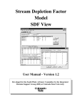
THE INTEGRATED DECISION SUPPORT CONSUMPTIVE
USE MODEL WORKSHOP
Copyright
Copyright © 2005 Integrated Decision Support Group
Civil Engineering Department
Colorado State University
Fort Collins, CO 80523-1372 USA
For more information contact:
Luis Garcia
Colorado State University
Fort Collins, CO 80523-1372 USA
Phone: (970) 491-5144
Fax: (970) 491-7626
E-mail: [email protected]
Web site: www.ids.colostate.edu
Introduction to IDSCU and Its Capabilities
1
INTRODUCTION TO IDSCU AND ITS CAPABILITIES
During this portion of the workshop, you will become familiar with the basic functions of
the IDSCU software by modeling a sample farm. You will be running the model starting
with a template to determine the consumptive use (CU) of a well. The information for the
sample farm is:
Farm
• The name of the farm is IDS Farm.
• It is located near Crook, Colorado, latitude 40.83 degrees.
• Its elevation is 3800 feet.
Crops
•
•
•
100 acres of corn (grain) are irrigated using a sprinkler with a 0.85
application efficiency on sandy soil.
40 acres of alfalfa are irrigated using a sprinkler with a 0.85 application
efficiency on clay soil.
20 acres of alfalfa are flood irrigated with a 0.5 application efficiency on
loam soil.
Water Supplies
•
•
•
5 shares of Pawnee Ditch (461.7 total shares) with a 0.7 conveyance
efficiency.
90 shares of Prewitt Pawnee (4900.2 total shares) with a 0.7 conveyance
efficiency.
1 Well with a decreed SDF of 480 and a max flow of 1,000 GPM.
A Reminder about IDSCU Help
Whenever you are working with the IDSCU Model, online help is
available. When you click on Help on the Menu bar, you will have
access to the latest IDSCU User’s Manual. You can search the Manual
using the table of contents, the index, or the find feature.
Introduction to IDSCU and Its Capabilities
2
GETTING STARTED
1. Click on your computer’s Start menu button. Choose Programs from the menu.
Choose IDSCU Model from the list of programs. Open the IDSCU Model.
2. Click on the File menu and select New. You can also select the first item in the
toolbar that looks like a blank page
.
3. A dialog box will pop up in front of the Consumptive Use input page. Select the
example.tcmn file from the list of templates and click OK.
4. The input screen will appear that has been initialized from the template.
What is an IDSCU template?
A template file contains information about the location being modeled. For
example, the template may contain information about crop characteristics such
as planting dates; weather data from local stations; and local surface water
diversion records. IDSCU templates always have a .tcmn extension.
Introduction to IDSCU and Its Capabilities
3
Introduction to IDSCU and Its Capabilities
4
ET METHODS
Halfway down the left side of the Input Screen is the ET Methods box. The IDSCU
Model allows you to select one or more monthly or daily methods for estimating ET. The
following monthly ET methods are available:
•
SCS Blaney-Criddle—This is a monthly method that was developed initially by the
Natural Resources Conservation Service (formerly the Soil Conservation Service). It
uses only mean temperature and precipitation. A sprinkler spray loss can be entered
for sprinkler irrigation systems; this factor is applied to the IWR (Irrigation Water
Requirement) for specified fields in the project area.
•
Calibrated Blaney-Criddle—The Blaney Criddle method can be used with
calibration factors (i.e. monthly multipliers) that you set by clicking on the Set BC
Coefficients button.
•
Pochop—The Pochop method is a modified version of the Blaney-Criddle method
that uses elevation and temperature adjustments for Kentucky bluegrass and alfalfa.
•
Hargreaves—The Hargreaves method was derived from 8 years of cool-season grass
lysimeter data from Davis, California. The method is recommended to calculate
weekly or longer time period ET (grass related reference (ETo)). The method
requires daily minimum and maximum temperature values.
Introduction to IDSCU and Its Capabilities
5
IDSCU offers the following daily methods for estimating ET:
•
ASCE Standarized Reference Evapotranspiration Equation—ASCE convened a
task force to established and define a benchmark
reference evapotranspiration equation. The
purpose of this new equation is to standardize the
Why are the daily
calculation of reference evapotranspiration that
can be used to improve transferability of crop
methods unavailable
coefficients.
•
Penman-Monteith Equations—Often used to
compute daily or hourly ET, the equation
combines an energy component and a mechanism
to remove the water vapor, with aerodynamic and
surface resistance terms.
•
Kimberly-Penman—This equation combines an
energy component and a mechanism to remove
water vapor with a variable wind function.
for some data sets?
If you select a template that
only has monthly data then
the daily ET methods will
be inactive and appear
grayed out. If you use a
template that has daily
data, the daily ET methods
would be active.
For this first example, you will reduce processing time by choosing only the number of
ET Methods you are interested in. For this example make sure that the Blaney-Criddle
and ASCE methods are checked.
Introduction to IDSCU and Its Capabilities
6
ADDING MODELING AREA INFORMATION
Now you will begin to enter specific information about the sample farm.
Farm
• Name of the farm is IDS Farm
• Latitude of 40.83 degrees (near Crook, Colorado)
• Elevation 3800 ft
Crops
•
•
•
100 acres of corn (grain) irrigated with a sprinkler with a 0.85 application
efficiency on sandy soil with an avg. water holding capacity of 1.0 in/ft.
40 acres of alfalfa irrigated with a sprinkler with a 0.85 application
efficiency on clay soil with an avg. water holding capacity of 2.0 in/ft.
20 acres of alfalfa, flood irrigated with a 0.5 application efficiency on clay
loam soil with an avg. water holding capacity of 1.7 in/ft.
1. Click on the Modeling Area Info button, in the bottom right corner of the Input
Screen. The Modeling Area Data screen pops up.
2. Click on the Add Modeling Area button on the right hand side of the screen. A
table in which to enter information about the new farm will appear at the top of
the screen.
Introduction to IDSCU and Its Capabilities
7
3. Click in the Modeling Area Name field and type in the name “IDS Farm”. Enter
the farm’s latitude (40.83) and elevation (3800 ft).
4. Click on the Add Field button near the bottom of the screen. A blank data entry
line will appear in the lower data entry table. You will be entering three different
fields as you have three areas of the farm that are cultivated differently (different
crops, soil types, or irrigation practices).
•
Double-click in the crop type cell for this field in the lower data entry
area. Select CORN_GRAIN from the list of crops.
Introduction to IDSCU and Its Capabilities
8
•
Double-click in the soil type cell for this field and choose SAND.
•
Type in an Application Efficiency of .85.
•
Put “No” for Sprinkler Spray Loss by double-clicking in the cell so it
toggles between yes and no.
•
Put “No” for Flood? as the crop is not flood irrigated.
•
Enter 100 acres in the first year of record (1992) and hit the return key;
this will cause the subsequent years to fill in with the same value.
•
Repeat the steps to input data for alfalfa.
♦
40 acres of Alfalfa (Sprinkler); CLAY; Application Efficiency .85
♦
20 acres of Alfalfa (Flood); LOAM; Application Efficiency .5
Introduction to IDSCU and Its Capabilities
9
When you are finished, your Modeling Area Data screen should look like this:
4. Click OK to accept your input.
Introduction to IDSCU and Its Capabilities
10
ASSIGNING WATER SUPPLIES
You are ready to assign the water supplies to the farm. IDS Farm’s water supplies consist of:
•
•
•
5 shares of Pawnee Ditch (461.7 total shares) with a 0.7 conveyance
efficiency.
90 shares of Prewitt Pawnee (4900.2 total shares) with a 0.7 conveyance
efficiency.
1 Well with a decreed SDF of 480 and a max flow of 1,000 GPM.
To assign water supplies to each farm, you will need to use the Surface Supplies and Well Information
buttons on the main CU screen. If the buttons are not active, make sure that you have checked the Use
Water Supply Data checkbox on the main CU screen.
TO ASSIGN SURFACE SUPPLIES
1. Click on the Surface Supplies button.
2. The Water Supplies screen pops up. The Current Modeling Area box indicates that
we are dealing with the IDS Farm.
3. Radio buttons allow you to switch between different Water Distribution Modes.
Select Pro-rated Flow.
4. Next click the New Ditch button. A list of ditches pops up. The water supply
information for IDS Farm indicates that you have shares in both Pawnee Ditch and
Prewitt Pawnee Ditch, so you will be entering two different ditches. Click on
Prewitt_Pawnee Ditch and hold down the control button while clicking on Pawnee
Ditch. Click OK to accept the ditches.
5. Back on the main Surface Supplies screen, make sure that Farm Allotment Varies
by Year is clicked OFF and Pro-rate surface water is clicked OFF.
Introduction to IDSCU and Its Capabilities
11
6. In the Ditch/Reservoir table, you will indicate the number of shares that IDS Farm is
allotted from each source:
Pawnee Ditch: Farm Allotment of 5.
Prewitt Pawnee: Farm Allotment of 90.
7. Click on the OK button, and the pop-up window will close.
Introduction to IDSCU and Its Capabilities
12
TO ASSIGN WELL INFORMATION
1. Click on the Well Information button on the main CU screen. The Well Information
screen will pop up.
2. The Well Information screen will indicate that you are modeling IDS Farm.
3. Choose Based on Decreed Location from the SDF Type pull down menu.
4. Select the No Water Shortage Allowed radio button from the choices offered in the
Consumptive Use of Groundwater Calculation Mode box. This means that the wells
on the farm will pump enough water to satisfy the demand of the crops after surface
supplies have been applied.
5. Click the Add button on the right side of the screen. A new well will appear in the
Well Information Table.
6. In the Well Information Table type:
• “IDS Well” under Well Name
• “1” under Fraction of Farm Supplied
• type “1000” under Max Flow
• type “480” under Decreed Location SDF.
Introduction to IDSCU and Its Capabilities
13
7. Click on the OK button, and the pop up window will close.
Introduction to IDSCU and Its Capabilities
14
ASSIGNING WEATHER INFORMATION
Now you will assign weather stations to the
farm.
1.
Click on Weather Stations to bring up
the weather stations dialog.
2.
Locate the Crook weather station and
enter a “1” under the IDS Farm column.
3.
Click OK to accept your changes.
Introduction to IDSCU and Its Capabilities
What if my farm is between several
weather stations?
If your farm is located between several
weather stations, you can select all of the
weather stations in the vicinity and prorate
them. The sum of the weather stations
should be “1” otherwise the “Farm 1”
column on the weather stations screen will
be highlighted in red and you will get an
error message when you try to run the
model.
15
RUNNING THE MODEL
1. Click on the
icon on the toolbar. Choose a name and a location for the project.
2. The model will run and a window showing the status of the run is shown on the
screen.
What do you mean I have an error?
When you run the model, you may get an error message saying that you have
no weather data for a particular year or that the efficiency for a particular
field has not been set. You need to go back to the main input screen, click on
the Weather Data button or the Modeling Area button to confirm this. You
can either reduce the number of years of simulation or fill any missing data.
Then click Run again.
3. The model will run and a blank results screen will appear.
4. To see the depletion of all water supplies, select IDS Farm for your modeling area
and choose the year or years of interest.
Introduction to IDSCU and Its Capabilities
16
5. You can plot the Total Depletion of Water Supplies using a Bar Chart or an XY
Graph.
6. To see the depletion of the well, click on Ground Water. The CU of Ground Water
dialog will appear. Choose a time scale, the farm, the well, and the years of interest
in the list boxes. The consumptive use of groundwater for that well will be displayed
in the table below.
Introduction to IDSCU and Its Capabilities
17
7. You can plot the CU Met by Ground Water as a Bar Chart.
Introduction to IDSCU and Its Capabilities
18
OTHER OPTIONS
In this section of the workshop, you will learn other ways that you can use IDSCU to assist you in inputting
data. Water, crop, and weather data can all be manipulated using options given on the main input screen.
Return to the input screen by clicking on the Window pull-down menu and selecting the
.cmn file or by clicking on the Close button at the bottom of the output screen.
INITIAL CONDITIONS
The Initial Conditions button is located in the bottom left corner of the screen. When
you click on it, the Initial Conditions pop-up opens which allows you to include winter
carry-over soil moisture in your calculations. Winter carry-over soil moisture is the
amount of winter precipitation that will be available to crops in the spring. The extra soil
moisture will contribute to the water available during the growing season, lowering the
amount of surface or ground water required.
You can either use a portion of the precipitation during the non-growing season to determine the amount of
soil water at the start of the next season or you can specify a fraction of the soil profile that is filled at the
beginning and end of each season.
What does MaxAllowSW mean?
MaxAllowSW stands for Maximum Allowed Soil Water and refers to the amount of
the water that can be stored in the soil profile for plant use. MaxAllowSW equals MAD
(Management Allowed Depletion) multiplied by maximum root depth multiplied by
AWC (Available Water Holding Capacity).
•
Wi
nter Precipitation Carry-Over - Most of the precipitation during the non-growing season falls as
snow. However, not all of the water from snowmelt will be available for storage in the soil since
Introduction to IDSCU and Its Capabilities
19
•
some of the snow will be sublimated. The fraction of winter carry-over option specifies the
percentage of winter precipitation that is available for storage each year. The fraction MaxAllow
SW at the start of the simulation period is the largest amount of soil moisture that can be
accumulated.
Fraction of MaxAllowSW at the Beginning and End of the Season - Alternatively, the fraction
of the soil profile filled at the beginning and end of each season can be specified. If the “No
Shortage” option is selected in the Well Information window, the wells will pump to fill the
profile to the specified end of season fraction.
Introduction to IDSCU and Its Capabilities
20
PRECIPITATION METHODS
Crops cannot make use of every drop of rain that falls because a portion will either run
off or percolate through the soil; the amount of rain that can be absorbed by the crop is
called the effective rain. The upper right hand side of the Consumptive Use window
provides two precipitation methods that can be used to estimate effective rainfall.
•
USBR (United States Bureau of Reclamation) - This method is based on U.S. Bureau
of Reclamation methodology in which effective rainfall is linearly related to average
monthly rainfall depending on intensity.
For the USBR method, if precipitation is:
< 1.0 inch, effective rain is precip x .95
< 2.0 inches, effective rain is ((precip – 1.0) x .90) + .95
< 3.0 inches, effective rain is ((precip – 2.0) x .82) + 1.85
< 4.0 inches, effective rain is ((precip –3.0) x .65) + 2.67
< 5.0 inches, effective rainfall is ((precip – 4.0) x .45) + 3.32
< 6.0 inches, effective rainfall is (( precip – 5.0) x .25) + 3.77
> 6.0 inches, effective rainfall is ((precip – 6.0) x 0.05) + 4.02
•
SCS (Soil Conservation Service) - This method is based on the SCS methodology in
which effective rainfall is dependent on the net depth of application and the average
monthly consumptive use.
Introduction to IDSCU and Its Capabilities
21
Table 1 SCS Method Table showing average monthly rainfall as related to mean monthly rainfall
and average monthly consumptive use.
Only one precipitation method can be selected at a time. For either method, the use
excess effective rainfall option impacts the soil moisture budget when rainfall is in
excess of consumptive use by allowing excess effective rainfall to be stored in the soil.
WATER SUPPLY OPTIONS
Introduction to IDSCU and Its Capabilities
22
Half way down the right side of the IDSCU input screen, you will see water supply options. There are
several options that can be set to regulate the use of water for a model run:
•
CU to be met for alfalfa or pasture acreage - If alfalfa and pasture fields in the area being modeled
are typically water limited, the CU of these two crops can be multiplied by the fraction you specify (a
value between 0 and 1).
•
Use Water Supply Data - You can elect to use water supply information by selecting the Use Water
Supply Data check box. If this option is selected, the water supply data from surface and ground water
will be used to determine shortages and excesses. Otherwise, only precipitation will be used to
calculate potential CU.
•
Calculate Recharge from Ditches and Wells - If checked, then deep percolation and runoff of water
supplies can be modeled as recharge sites. The first step is to indicate what portion of deep percolation
and runoff is deep percolation. Water that is deep percolated will return to the river via ground water;
the impact to the river will be according to the farm or ditch’s SDF value. Runoff will return to the
river via surface water routes. The next step is to assign application efficiencies for every well on the
farm; because the model can compute consumptive use of ground water, this application efficiency
will be used to generate the gross pumping for the well. The difference between the gross pumping and
the water used in consumptive use will be modeled as surface and ground water recharge. The check
boxes on the bottom allow the user to customize what types of recharge to model.
OTHER TYPES OF DATA FOR IDSCU
You will learn how to add weather and surface water data.
ADDING MONTHLY OR DAILY WEATHER DATA
Your current dataset was provided to you with a complete weather dataset. However
there might be instances were you want to update your dataset or add new weather
stations. To determine what are the current settings for your dataset are follow this steps.
1. Click on the “P” in the toolbar or by selecting Properties from the Model
Options menu. The following pop-up screen will appear.
Introduction to IDSCU and Its Capabilities
23
2. In the event that you had a Monthly dataset you would Click the Daily check box
and hit OK. This would create space in the project for daily input data.
3. The dataset that we have been working with contains Northern Colorado Water
Conservancy District (NCWCD) and COlorado AGricultural Meteorological
nETwork (COAGMET) weather stations. In order to update the weather data you
need to follow the following steps:
NCWCD
a) Click on Edit Weather Data on the main IDSCU screen. Select the station
you are going to add data to by clicking on the weather station name
(NCWCD CROOK 109) from the existing list of weather stations. This will
set NCWCD CROOK 109 as the current station being edited.
b) Add and/or update the weather data by clicking the NCWCD button next to
Import Weather for station NCWCD CROOK 109 (the name of the
selected station is shown). If you connected to the internet the IDSCU
program will access the NCWCD site and display the following pop-up:
Introduction to IDSCU and Its Capabilities
24
c) Select the NCWCD station you want to obtain data for and press OK. The
program will automatically download the data for this station for all the years
of your dataset (limited by the weather station period of record).
COAgMet
d) Using a web browser go to the COAgMet web site
(http://ccc.atmos.colostate.edu/~coagmet/) and select Raw Data Access
(http://ccc.atmos.colostate.edu/~coagmet/rawdata_form.php). Select the start and
end date for the data you want to download (January 1, 1992 to December
31, 2004), the station name (FTM01 - Fort Morgan), daily data in new
format. Then press the Submit button at the bottom of the page. The
requested data will be displayed on the screen. Select Ctrl-a and Ctrl-c (to
copy all the data displayed on the screen) then save this information to a text
file on your computer by opening a new text file in wordpad and pressing
Ctrl-v. Then save the file as c:\temp\ft_morgan_coagmet.txt.
e) Now add this data to the IDSCU by clicking on Edit Weather Data. Select
the station you are going to add data to (CoAgMet FORT MORGAN).
f) Add the weather data you just downloaded by clicking the CoAgMet button
next to Import Weather for station CoAgMet FORT MORGAN. This will
brings a file selection dialog. Surf to the location of the file that you
downloaded (c:\temp\ft_morgan_coagmet.txt) and select the file.
4. NOTE: When using daily weather data, the height of the temperature and wind measuring
instruments NEEDS to be specified. The standard heights for NCWCD are: 4.96 feet for
temperature measurement height and 8.2 feet as the wind measurement height and for COAgMet
they are 4.96 feet for temperature measurement height and 6.56 feet as the wind measurement
height
5. Save your changes by hitting the OK button at the bottom of the screen.
Introduction to IDSCU and Its Capabilities
25
CHECKING CROP COEFFICIENT DATA
We should check to make sure that we have crop coefficient data available, especially
when new ET methods have been added to the project. Click the Crop Coefficients
button to view the crop coefficients.
The pull-down list at the top shows all the crop types available to the model.
1. Select CORN_GRAIN and the Blaney-Criddle crop coefficients will be
displayed.
2. Click on Grass/Alfalfa Reference radio button to view the crop coefficient
values for the reference crop based ET methods. You have the choice of using
grass or alfalfa as the reference crop.
3. In this case, you should select Use Alfalfa as the coefficients in this dataset are
for alfalfa.
4. Click OK to save your changes.
Introduction to IDSCU and Its Capabilities
26
CHECKING CROP CHARACTERISTICS
We should also check to make sure that the crop parameters look reasonable for the area
we are modeling. Click on Crop Characteristics to bring up the crop and soil editor
window. Each column in the crop characteristics table represents a crop parameter.
The information in this table is particularly important with respect to specifying the start,
end, and length of the growing season. The planting and harvest date of each crop is
based on the Spring Frost Method and the Fall Frost Method.
•
If the Spring Frost Method is set to Mean Monthly, then the planting date is
calculated to be the earliest date that the mean monthly temperature is greater than the
planting temperature during the spring (January through July).
•
In the case of harvest date calculation, the harvest date is the first day in the fall at
which the mean temperature reaches harvest temperature.
•
For the other two methods (published 28 degree frost dates and published 32 degree
frost dates), the 28 and 32 degree frost dates are already known for each weather
station and will be used as the earliest planting date and the latest harvest date.
•
If the crop has a planting date specified, then the model will use that unless the mean
temperature falls below the planting temperature after that date, in which case the day
that occurs will be the new planting date. The harvest date will be the planting date
plus the length of the season, unless the harvest temperature occurs before then, in
which case the earlier date will be used.
Save any changes you made by hitting OK.
Introduction to IDSCU and Its Capabilities
27
ADDING CROPS AND/OR SOIL TYPES
The model normally has three types of soils: Sand, Clay and Loam. The soil type is
important because it is used when doing a soil moisture budget. The average water
holding capacity (in/ft) is multiplied by the root zone and the management allowable
depletion (MAD) to available soil moisture. To add a new soil type click on the New Soil
button as shown below.
A new soil will be added with the name “New_Soil”. You can change the name of the
soil and enter a value for the average water holding capacity. Change the name of the
new soil to CLAY LOAM and assign an average water holding capacity (in/ft) of 1.7.
Press OK at the bottom of the window to save the new soil type.
The IDS Farm had the following parcel:
•
20 acres of alfalfa are flood irrigated with a 0.5 application efficiency on loam
soil.
If we are told that the soil type is now clay loam instead of loam we need to change this
information in the Modeling Area Info window which we can access from the main
IDSCU window. Select the Modeling Area Info button, select the IDS Farm (when you
have multiple farms only the parcel information for the selected modeling area is
displayed in the field table at the bottom of the window). Click on the soil type for the
Alfalfa field and from the pop-up window select “clay loam”. This will update the soil
type associated with that field. Click OK at the bottom of the window to save the
information.
Introduction to IDSCU and Its Capabilities
28
EDITING SURFACE DATA
You will now learn how to add water supplies using the Hydrobase Access interface.
1. Click on the Edit Surface Data button and the Surface Water Editor Screen will pop
up.
2. The template that you used for generating the input data already has a lot of the
diversion records for ditches developed. In order to develop our own diversion
records we will remove all pre-existing ditch diversion records. To accomplish this,
click Delete Ditches and select all the ditches in the list: the easiest way to do this is
to click on the top entry and drag the mouse down the list until all the entries are
highlighted. Click the OK button.
Introduction to IDSCU and Its Capabilities
29
3. Next in the Database Function area in the window type "Pawnee" into the Name
Filter box and click on the Add Ditch from Hydrobase button. You may need to
surf to the location of the Hydrobase database (in this case we will be using
HB_DIV1.mdb located in u:\ids).
4. The Add Ditch from Database pop-up window will open. Choose “(1) Irrigation”
from the pull-down list of ditch uses to limit ditch entries that have a use of type
irrigation.
Introduction to IDSCU and Its Capabilities
30
5. Four items will appear for Pawnee in the list of entries. There are two items that have
Prewitt Reservoir in the “From” column. Select the two items that DO NOT have
Prewitt Reservoir listed in the “From” column by clicking in the name column for
those records that you want to add with your mouse while holding down the control
key on your keyboard.
6. Click OK. The combined diversion (for the two records that you retrieved from the
database) for Pawnee ditch will appear in the list of ditches on the Surface Water
Editor screen.
7. Add the Prewitt diversion record by again clicking on the Add Ditch from
Hydrobase button. Choose “(1) Irrigation” from the pulldown list of ditch uses.
Select the two items that HAVE Prewitt Reservoir in the “From” column by clicking
in the name column for those records that you want to add with your mouse while
holding down the Control key on your keyboard.
8. By default the interface uses the name of the first record from the database as the
name of the surface water supply. In order to differentiate the two diversion records,
you should change the name on the second entry by typing in the Ditch/Res Name
field in the table and entering PREWITT_PAWNEE DITCH.
9. Hydrobase does not provide total ditch share or conveyance efficiency information,
so we will need to add that ourselves.
•
For the PAWNEE DITCH, type “461.7” in the total column and “0.7” in the
application efficiency column.
•
For the PREWITT_PAWNEE DITCH, type “4900.2” in the total column
and “0.7” in the application efficiency of column.
Your Surface Water Editor screen should now look like this:
Introduction to IDSCU and Its Capabilities
31
10. Click OK. A small pop-up screen will appear that asks you how to update the
diversion records associated with each modeling area. Select “Update all farm ditch
information” since we want all data associated with the ditches to be updated. NOTE:
In the event that you have entered different efficiencies for a ditch based on the
location of the modeling area, you will want to select “Only update flows” so that you
can maintain the different conveyance efficiencies. Click OK to return to the main
CU page.
Introduction to IDSCU and Its Capabilities
32
Surface Water Editor Pitfalls
If you changed the names of ditches that were assigned earlier to your modeling
areas, you will need to go to Surface Supplies to delete those ditches that
changed in each area and add the new ditches. This is because the original design
of the model stored surface water supplies with each modeling area, and it was
only recently that it was decided that it would be better to keep a single source of
all surface supplies. Therefore there is an extra step that updates modeling area
surface water supplies by looking for matches between ditches in the modeling
area with ditches in the surface water editor. In this case you DO NOT need to do
this because we maintained the same names.
USING IDCSU FOR FORECASTING AND RECHARGE
FORECASTING SCENARIOS
In this part of the workshop, you will be using IDSCU to model the effects of long-term drought. One way
to do this is to create weather and ditch data based on an existing period of drought in our data.
1.
Find the Synthesized End Year box in the main input screen.
2.
Enter “2013” and press return.
Introduction to IDSCU and Its Capabilities
33
3.
Since 2002 was an extremely dry year, you will repeat that year for ten years by clicking Use Given
Year and selecting 2002 from the pull-down list.
4.
Press OK to populate the new years of weather, crop acreage, and ditch data. If you want to rebuild
your synthetic data a different way, just repeat this process by selecting the (Re)Synthesize button.
Introduction to IDSCU and Its Capabilities
34
RUNNING THE MODEL WITH THE NEW CHANGES
1. Before we run the model, we need to check that our simulation years are correct. Since our daily
weather data starts at 2002, set the Simulation Year Range to start in 2002 and end in 2013.
2. Now that we have added daily data the model enables all the daily ET Methods
(ASCE, Penman-Monteith and Kimberly-Penman). For this simulation we will
select both Blaney-Criddle and ASCE as shown below.
3. Press the Run button.
4. Since you changed some data in the input file the model will prompt you to store the modified
data file in the same file name or create a new data file. Create a new file using the word “daily” in
the name.
5. While the model is running, a pop-up window displays a number of messages that show the status
of the run. Below is the status window that you should see when you run the dataset we are
working with.
Introduction to IDSCU and Its Capabilities
35
The output screen shows all the available ET methods in the upper left-hand corner. In addition there are
choices for including the effects of soil moisture. Since results can only be viewed for one ET method at a
time, the Water Budget, Ground Water, and Detailed ET windows will show results only for the
selected ET method and soil moisture option. For our purposes:
1. Click on ASCE.
2. Make sure the Without Soil Moisture button is selected.
3. Select IDS Farm from the Modeling Areas.
4. Select the years 2002 through 2006.
Introduction to IDSCU and Its Capabilities
36
THE WATER BUDGET OUTPUT SCREEN
1. On the main out put screen, select the ET method (ASCE) and the soil moisture option (Without
Soil Moisture) and click Water Budget.
2. The Water Budget window will open.
3. Select the Modeling Area, IDS Farm, and the year, 2002, to view results.
•
Data for multiple modeling areas and multiple years can be displayed simultaneously. Select check
boxes on the upper right of the window to add columns of data corresponding to the selected
items.
A Note About Data Display
You can display data in a monthly format in rows separated by years, or you can display data
by each data item with the months in columns and the years in rows. To change the format of
the data, select the box next to the Format Annually text above the data display window.
Column widths and row heights can be sized by left clicking on the dividers of the titles and dragging the
symbol to resize columns or the symbol to resize rows.
Water budget data can also be plotted.
Introduction to IDSCU and Its Capabilities
37
USING IDCSU FOR COMPARISON
COMPARISON OF ET METHODS
Close the various windows until you reach the main water budget window.
Click Compare.
Introduction to IDSCU and Its Capabilities
38
Select the two desired ET methods to compare and select the Time Scale, Modeling Areas and options
desired. You will also need to choose whether you want to compare CU or irrigation water requirement.
To show the ratio of the two methods select the Ratio box. This will display the first method divided by the
second. You can change the order of the two methods in the selection boxes at the top of the window to
invert the ratio.
You can display the table data in wordpad, save the table to a text file, or plot the results of the comparison
by using the buttons along the bottom of the window.
Introduction to IDSCU and Its Capabilities
39
ALLUVIAL WATER ACCOUNTING SYSTEM
Now we can see how the wells we modeled in IDSCU will impact the river. From the Functions menu
select Export Wells to SDView/AWAS.
Introduction to IDSCU and Its Capabilities
40
On the left side are the available ET methods, and on the right you can select whether you want to include
the effects of soil moisture and what program you want to use.
1.
Under Export to make sure the radio button for AWAS is selected.
2.
Press OK and AWAS will open with every well in your dataset.
The good news is that if you want to use the SDF method in AWAS, you have a complete dataset without
having to do any work!
1.
Click the Run button on the toolbar.
2.
Save the dataset, and the model will calculate the effects of the well pumping on the river.
3.
Close the output text box, and at the top of the output screen choose Monthly from the time scale
section, IDS Well from the list of sites, and 2002-2005 from the list of years. The net pumping
and river depletion will be displayed in the table.
Introduction to IDSCU and Its Capabilities
41
You can plot the table data or save it to a file using the buttons at the bottom of the screen.
Set the timescale and select from the site and year lists what part of the data you would like to see. Show
CU of Ground Water/Net Recharge Data will display the input data for each site, and Show
Depletion/Accretion Data will display the impact on the river.
The next sections describe the input and output tabs in detail.
Introduction to IDSCU and Its Capabilities
42
THE PROPERTIES WINDOW
Clicking the Properties button on the input screen will display the project properties:
You may choose to display data using three year types:
•
•
•
Calendar Year - (January - December)
Irrigation Year - (November - October)
USGS Year - (October - September)
You can change the time scale to monthly, which will aggregate daily data to monthly values, or change
monthly values to average daily values.
If you change the starting or ending years, then either new un-initialized data will be added if the period of
record is increased or data will be removed if the period of record is decreased. If you want to initialize the
new data instead, then use the forecasting options by clicking Modify Forecasting Options, enter a new
year and click Forecast. The forecast options are identical to those in the IDSCU model.
Introduction to IDSCU and Its Capabilities
43
What is the deal with monthly mode and average days per month?
The AWAS model is designed to run using uniform time periods; therefore in order to create accurate
output, monthly data must be converted to average daily data using the number of days in each month.
However, this can increase the execution time of the model significantly, so it may be preferable to
have the model run using a time period of 30.42 days.
You may choose to limit the number of decimal places shown on the forecasted data by specifying a
precision.
If you want to forecast the effect of decreasing or increasing pumping into the future by a certain amount,
enter a monthly multiplier at the bottom of the Properties window.
Introduction to IDSCU and Its Capabilities
44
THE MAIN INPUT SCREEN
Near the top of the screen is a window containing all the sites in the dataset. Each site has several properties
that can be assigned:
1.
2.
3.
4.
5.
6.
7.
8.
9.
10.
11.
12.
13.
14.
Name - The name of the site.
Description - An optional description of the site.
Type - Either Irrigation or Recharge.
Boundary Condition - Either Infinite Aquifer, Alluvial Aquifer, No Flow, or Effective SDF.
W - The distance between the parallel no-flow boundary and the river. Used when Alluvial
Aquifer is set.
B - The distance between the well and the perpendicular no-flow boundary. Used when No Flow
is set.
Transmissivity - The ability of an aquifer to transmit water. Units are in gallons per day per foot.
Specific Yield - Related to porosity, it is the volume of water per unit volume of aquifer that can
be extracted by pumping.
X - The distance of the well to the river. Used by all boundary conditions except Effective SDF.
SDF - The stream depletion factor of the site. Used by Effective SDF.
Show In Output - If yes, then the site will be included in the model calculation. This is useful
when you want to create a model run that contains a subset of sites without having to create
additional datasets.
Use Partial Stream - If unchecked, the stream is considered to be infinite in length. If checked,
left and right stream lengths will be used instead.
Left Limit of Stream Segment - The distance from the point on the river that is closest to the
well to the left end of the river.
Right Limit of Stream Segment - The distance from the point on the river that is closest to the
well to the right end of the river.
The New Well and Delete Wells buttons will add and remove sites from the dataset.
The bottom table displays net pumping or recharge for the selected site. Sites are selected by clicking
anywhere in the site’s row in the site table.
The display can also show pumping or recharge record information, but at this time the record calculator is
experimental and its use is not recommended.
Introduction to IDSCU and Its Capabilities
45
Table Functions
Every table in IDSCU and AWAS use a common set of keyboard shortcuts for copying and editing
of data. In every case the function operates on the selected cells in the table in a manner similar to
Excel. To make a selection, click on the upper left corner of the region you want to highlight and
hold down the left mouse button. Next drag the mouse to the lower right corner of the region and
release the button. A region can also be selected by selecting a cell, and then while holding down
the shift key, selecting another cell. This will highlight all the cells between the two clicked cells.
Individual cells can be selected by clicking on cells while the control key is pressed.
The following functions are available:
• Ctrl-A Select every cell in the table.
• Ctrl-C Copy every selected cell to the clipboard.
• Ctrl-V Paste the clipboard into the table. If only one cell is selected, then the cells are
pasted starting at the selected cell and moving to the right until a copied row is complete,
at which point the next row is started. The result is that the shape of the copied region is
preserved. If a region is selected in the destination table, then the paste will fill the region.
If the destination region is larger than the copied region, it will by filled by repeating
copied cells. This is most often used when you want to set all the cells in a table to a
single value.
Once the well parameters and net pumping/recharge are entered, the model is nearly ready to run. The start
and end dates of the model will default to the period of record, but you can change how the model uses the
input by altering the parameters at the bottom of the input screen:
The start of the simulation can be set to occur after the beginning of the dataset if you want to ignore the
first years of the dataset.
The model can also be set to stop before the end of the period of record or to continue beyond the end of
the dataset, in which case the sites are assumed to not pump or recharge; this is useful when you want to
see the how the river continues to deplete even when pumping stops.
To ignore the last years of the dataset, enter a month and year in the Ignore pumping/recharge after
section.
Click Run to run the model with your new input.
Introduction to IDSCU and Its Capabilities
46
THE OUTPUT SCREEN
Click the Run icon to run the model using the dataset imported from IDSCU.
When the model run is complete, close the model output message screen.
The output screen will now appear. At the top left is the daily or monthly time scale setting. Next is the site
selection window. Any sites that were set to show an output will appear in the list, as well as four
additional selections:
1.
2.
3.
4.
Total of Selection: This creates an artificial site that contains the sum of the selected sites. This is
useful for calculating the net effect of a portion of the dataset.
Recharge Summary: This will show the net recharge and accretion of all the recharge sites in the
output.
CU of Ground Water Summary: This will show the net CU of ground water and river depletion
of every irrigation site in the output.
Net Impact on Stream: This is the sum of all depletions and accretions on the river.
Next choose the period of record you want to see. Drag the mouse over the year entries, or click one year
and while holding down the shift key select another year to select a continuous group, or click while
holding the control key down to pick individual years.
The output table will now show the model results constrained by your site and year selections. The model
input and output can be displayed or hidden as follows:
•
•
Show CU of Groundwater/Net Recharge Data: This is the input data that the model used.
Show Depletion/Accretion Data: This is the output of the model, the impact of the irrigation or
recharge site.
Introduction to IDSCU and Its Capabilities
47
There are several formatting options available as well:
•
•
Standard: Table data will be displayed using a row containing the name of the site or summary
option and a row for each year of data.
Spreadsheet: This creates a tab-delimited text file formatted in ways that make display in Excel
easier. The spreadsheet will also contain all the information necessary for AWAS to generate a
new dataset. A text file created using this option can be read in by choosing the text file type from
the file selection dialog when opening a new dataset.
The following options modify the spreadsheet style:
•
•
•
Open in Excel: The resulting text file will be opened in Excel.
Depletions are Positive: All net pumping and depletions will be set to positive values. The user
will have to consider whether the site is irrigation or recharge when performing any analyses.
Compact Format: When this option is turned off, only the net pumping and depletions will be
saved to the text file.
To update an existing AWAS project with changes you made to an AWAS generated spreadsheet, select
Add To Project from the File pull-down menu and choose the spreadsheet text file. If the name of the text
file is the same name as the dataset but with a .txt extension instead of .dsi extension, you can open the text
file directly using the Open menu item and changing the Files of Type selection at the bottom of the file
dialog to AWAS Import Files.
Introduction to IDSCU and Its Capabilities
48
CREATING A DATASET USING GLOVER PARAMETERS
Now we will consider a more complex alternative to using SDF that instead uses aquifer parameters.
Suppose that our well has the following aquifer parameters:
•
•
•
•
The distance of the well to the river is 8,108 feet.
The distance of the well to the boundary is 3,549 feet.
The transmissivity of the aquifer at the well is 115,400 gallons per day per foot.
The specific yield of the aquifer at the well is 0.2.
1.
For comparison purposes, we will create another well by clicking on the New Well
button.
2.
Enter a description for the well IDS Well – aquifer.
3.
Change the boundary type to Alluvial Aquifer and enter the total distance from the river
to the boundary in the W column (11,657), the value for transmissivity (115,400),
specific yield (0.2), and the distance from the well to the river in the X column (8,108).
4.
To copy the original well pumping to the new well, select the original well in the top
table by clicking on its name so that its pumping is displayed in the bottom table.
5.
Click the mouse in the pumping table and type Ctrl-a to select all the cells and Ctrl-c to
copy them to the clipboard.
6.
Now select the new well from the top table and then click in the first cell of the pumping
table. Click Ctrl-v to paste the pumping records.
It would be nice to see how each method behaves when pumping stops, so let’s set the model to run to the
year 2020 by entering 2020 in the To box.
Click the Run button, save the dataset, and close the output window. Select Monthly as the time scale, the
two wells in the site list, and all the years in the year list. Click Plot to see the pumping and depletion for
each site.
Introduction to IDSCU and Its Capabilities
49
The depletions of the well for which you entered the alluvial aquifer parameters are showing that the
impact on the stream is more immediate than the SDF well. However, much of the difference can be
attributed to the fact that we used the point transmissivity at the well instead of using a harmonic mean to
compute the transmissivity along the flow path to the river. For this example the harmonic mean for this
site has a transmissivity of 59,800 gallons per day per foot. Let’s add a third well that uses this value and
see how it impacts our results.
1.
Click on the New Well button.
2.
Enter a description for the well IDS Well – low trans.
3.
Change the boundary type to Alluvial Aquifer and enter the total distance from the river to the
boundary in the W column (11,657), the value for transmissivity (59,800), specific yield (0.2), and
the distance from the well to the river in the X column (8,108).
4.
To copy the original well pumping to the new well, select the original well in the top table by
clicking on its name so that its pumping is displayed in the bottom table. Click the mouse in the
pumping table and type Ctrl-a to select all the cells and Ctrl-c to copy them to the clipboard. Now
select the new well from the top table and then click in the first cell of the pumping table. Click
Ctrl-v to paste the pumping records.
Introduction to IDSCU and Its Capabilities
50
Click the Run button, save the dataset, and close the output window. Select Monthly as the time scale, the
three wells in the site list, and all the years in the year list. Click Plot to see the pumping and depletion for
each site.
Introduction to IDSCU and Its Capabilities
51
The graph shows the expected timing of the depletions on the river. It can be seen from the graph that the
fastest impact is for the point transmissivity, followed by the harmonic mean transmissivity and the slowest
impact is that of the SDF.
Introduction to IDSCU and Its Capabilities
52