Download ARMSTRONG`S PHASE MODULATOR

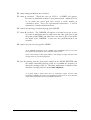
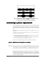
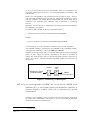
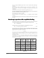
ARMSTRONG'S PHASE
MODULATOR
PREPARATION............................................................................... 106
FM generation ......................................................................... 106
Armstrong`s modulator ........................................................... 107
theory....................................................................................... 107
phase deviation........................................................................ 108
practical realization of Armstrong`s modulator ...................... 109
EXPERIMENT ................................................................................. 110
patching up .............................................................................. 110
model adjustment .................................................................... 110
Armstrong's phase adjustment................................................. 112
phase adjustment using the envelope......................................................112
phase adjustment using ‘psycho-acoustics’ ............................................112
practical applications............................................................... 113
spectral components ................................................................ 113
TUTORIAL QUESTIONS ............................................................... 116
APPENDIX....................................................................................... 117
Analysis of Armstrong`s signal ............................................... 117
the amplitude limiter ..............................................................................117
Armstrong`s spectrum after amplitude limiting......................................118
Armstrong's phase modulator
Vol A2, ch 12, rev 1.1
- 105
ARMSTRONG'S PHASE
MODULATOR
ACHIEVEMENTS: modelling Armstrong's modulator; quadrature phase
adjustment; deviation calibration; introduction to the amplitude
limiter.
PREREQUISITES: earlier modulation experiments; an understanding of the
contents of the Chapter entitled Analysis of the FM spectrum in this
Volume.
EXTRA MODULES: SPECTRUM UTILITIES; 100 kHz CHANNEL FILTERS
(optional).
PREPARATION
FM generation
As its name implies, an FM signal carries its information in its frequency variations.
Thus the message must vary the frequency of the carrier.
Spectrum space being at a premium, radio communication channels need to be
conserved, and users must keep to their allocated slots to avoid mutual interference.
There is a conflict with FM - the carrier must be maintained at its designated centre
frequency with close tolerance, yet it must also be moved (modulated) by the
message.
A well know source of FM signals is a voltage controlled oscillator (VCO). These
are available cheaply as integrated circuits. It is a simple matter to vary their
frequency over a wide frequency range; but their frequency stability is quite
unsatisfactory for today`s communication systems. Refer to the experiment entitled
Introduction to FM using a VCO in this Volume.
Armstrong`s modulation scheme 1 overcomes the problem 2. It does not change the
frequency of the source from which the carrier is derived, yet achieves the objective
by an indirect method. It forms the subject of this experiment.
1 Armstrong`s system is well described by D.L. Jaffe ‘Armstrong`s Frequency Modulator’, Proc.IRE,
Vol.26, No.4, April 1938, pp475-481.
2 but introduces another- it is not capable of wide frequency deviations
106 - A2
Armstrong's phase modulator
Armstrong`s modulator
Armstrong's modulator is basically a phase modulator; it can be given a frequency
modulation characteristic by an integrator inserted between the message source and
the modulator. For a single tone message, at one frequency, it is not possible to tell,
by what ever measurement, if the integrator is present (so it is an FM signal) or not
(a PM signal). Only with a change of message frequency can one then make the
decision - by noting the change to the spectral components, for example.
theory
You are already familiar with amplitude modulation, defined as:
AM = E.(1 + m.sinµt).sinωt
...... 1
This expression can be expanded trigonometrically into the sum of two terms:
AM = E.sinωt + E.m.sinµt.sinωt
...... 2
In eqn.(2) the two terms involved with 'ω' are in phase. Now this relation can easily
be changed so that the two are at 90 degrees, or 'in quadrature'. This is done by
changing one of the sinωt terms to cosωt. The signal then becomes what is
sometimes called a quadrature modulated signal. It is Armstrong`s signal.
Thus:
Armstrong`s signal = E.cosωt + E.m.sinµt.sinωt
...... 3
α= 0
α = 90 o
Em
Em
2
2
Em
2
E
E
E
m= 1
Em
2
Em
m= 1
(a)
2
(ω-µ) ω (ω+ µ)
(b)
Phasor Form
Em
2
frequency
Amplitude Spectrum
Figure 1: DSBSC + carrier
The signals described by both eqn. (2) and eqn. (3) are shown in phasor form in
Figure 1 (a) and (b) above. The amplitude spectrum is also shown; it is the same for
both cases (a) and (b).
Each diagram shows the signals for the case m = 1. That is to say, the amplitude of
each side frequency component is half that of the carrier.
In the phasor diagram the side frequencies are rotating in opposite directions, so
their resultant stays in the same direction - co-linear with the carrier for (a), and in
phase-quadrature for (b).
Both eqn. (2) and eqn. (3) can be modelled by the arrangement of Figure 2 below.
Armstrong's phase modulator
A2
- 107
DSBSC
message
(sine wave)
g
Armstrong`s
signal
G
100 kHz
(sine wave)
carrier
adjust phase
Figure 2: Armstrong`s phase modulator
phase deviation
Having defined Armstrong`s signal it is now time to examine its potential for
producing PM.
But first: we have been using the symbol ‘m’ for the ratio of DSBSC to carrier
amplitude, because our starting point was an amplitude modulated signal, and ‘m’
has been traditionally the symbol for depth of amplitude modulation.. The amplitude
modulation was converted to quadrature modulation. We will acknowledge this in
the work to follow by making the change from ‘m’ to ‘∆φ’. Thus:
........ 4
∆φ = m
Analysis shows (see the Appendix to this experiment) that the carrier of Armstrong`s
signal is undergoing phase modulation.
The peak phase deviation is proportional to the ratio of DSBSC to CARRIER peak
amplitudes at the ADDER output; but it is not a linear relationship. The peak phase
deviation, ∆φ, is given by:
∆φ = arctan [
DSBSC
] radians
CARRIER
...... 5
Remember that the amplitude of the DSBSC is directly proportional to that of the
message, so the message amplitude will determine the amount of phase variation.
For small arguments, arctan(arg) ≈ arg
Thus to minimize distortion at the receiver the ratio of DSBSC to carrier must be
kept small.
A receiver to demodulate a phase modulated signal is sensitive to these phase
deviations.
To keep the received signal distortion to acceptable limits the peak phase deviation
at Armstrong`s modulator should be restricted to a fraction of a radian, according to
distortion requirements as per Figure 3. The analysis of distortion is discussed in the
Appendix to this experiment.
108 - A2
Armstrong's phase modulator
Figure 3: distortion from Armstrong`s modulator
practical realization of Armstrong`s
modulator
The principle of Armstrong's method of phase modulation, or his frequency
modulator (with the added integrator as described earlier), is used in commercial
practice. But the circuitry employed to generate this signal is often not as
straightforward as the arrangement of Figure 2. It is not always possible to isolate,
and so measure separately, the amplitudes of the DSBSC and the CARRIER. So it is
not possible to calculate the phase deviation, in such a simple, straight forward
manner.
Amplitude limiters are also incorporated in the circuitry. These intentionally remove
the envelope, which otherwise could be used as a basis for measurement.
In these cases other methods must be used to set up and calibrate the phase deviation
of the modulator. These include, for example, the use of a calibrated demodulator.
There is also the method of 'Bessel zeros'. This is an elegant and exact method, and
is examined in the experiment entitled FM and Bessel zeros in this Volume.
Armstrong's phase modulator
A2
- 109
EXPERIMENT
patching up
In this experiment you will learn how to set up Armstrong`s modulator for a
specified phase deviation, and a unique method of phase adjustment.
Armstrong`s generator, in block diagram form in Figure 2, is shown modelled in
Figure 4 below.
CH1-A
ext. trig
CH2-A
Figure 4: the model for Armstrong`s modulator
T1 patch up the model in Figure 4. You will notice it is exactly the same
arrangement as was used for modelling AM. The major difference for
the present application will be the magnitude of the phase angle α zero degrees for AM, but 900 for Armstrong.
T2 choose a message frequency of about 1 kHz from the AUDIO OSCILLATOR.
model adjustment
T3 check that the oscilloscope has triggered correctly, using the external trigger
facility connected to the message source. Set the sweep speed so that
it is displaying two or three periods of the message, on CH1-A, at the
top of the screen.
Now pay attention to the setting up of the modulator. The signal levels into the
ADDER are at TIMS ANALOG REFERENCE LEVEL, but their relative
magnitudes (and phases) will need to be adjusted at the ADDER output.
To do this:
110 - A2
Armstrong's phase modulator
T4 rotate both g and G fully anti-clockwise.
T5 rotate g clockwise. Watch the trace on CH2-A. A DSBSC will appear.
Increase its amplitude to about 3 volts peak-to-peak. Adjust the trace
so its peaks just touch grid lines exactly a whole number of
centimetres apart. This is for experimental convenience; it will be
matched by a similar adjustment below.
T6 remove the patching cord from input g of the ADDER
T7 rotate G clockwise. The CARRIER will appear as a band across the screen.
Increase its amplitude until its peaks touch the same grid lines as did
the peaks of the DSBSC (the time base is too slow to give a hint of the
fine detail of the CARRIER; in any case, the synchronization is not
suitable).
T8 replace the patch cord to g of the ADDER.
At the ADDER output there is now a DSBSC and a CARRIER, each of exactly the
same peak-to-peak amplitude, but of unknown relative phase.
Observe the envelope of this signal (CH2-A), and compare its shape with that of the
message (CH1-A), also being displayed.
T9 vary the phasing with the front panel control on the PHASE SHIFTER until
the almost sinusoidal envelope (CH2-A) is of twice the frequency as
that of the message (CH1-A). The phase adjustment is complete when
alternate envelope peaks are of the same amplitude.
As a guide, Figure 5 shows three views of Armstrong’s signal, all with equal
amplitudes of DSBSC and carrier, but with different phase errors (ie, errors from the
required 900 phase difference between DSBSC and carrier).
Armstrong's phase modulator
A2
- 111
Figure 5: Armstrong’s signal, with ∆φ = 1, and phase errors of
45 deg (lower), 20 deg,(centre) and zero (upper).
Armstrong's phase adjustment
An error from quadrature at the transmitter will show up as distortion of the
recovered message at the receiver. This will be in ‘addition’ to the inherent
distortion introduced by the approximation arctan(arg) ≈ (arg). The ‘addition’ would
be anything but linear, and difficult to evaluate, but easy to measure for a particular
case.
How can the phase of the DSBSC and the added carrier be adjusted to be in exact
quadrature ?
An analysis of the envelope of Armstrong`s signal is given in the Appendix to this
experiment. There it is shown that:
1. when in phase quadrature, the envelope is sinusoidal-like in shape (Figure 5
above) with adjacent peaks of equal amplitude.
2. the envelope waveform is periodic, with the fundamental frequency being twice
that of the message from which the DSBSC was derived.
Each of these two findings suggests a different method of phase adjustment.
phase adjustment using the envelope
T10 trim the front panel control of the PHASE SHIFTER until adjacent peaks of
the envelope are of equal amplitude. To improve accuracy you can
increase the sensitivity of the oscilloscope to display the peaks only.
Equating heights of adjacent envelope peaks with the aid of an oscilloscope is an
acceptable method of achieving the quadrature condition. For communication
purposes the message distortion, as observed at the receiver, due to any such phase
error, will be found to be negligible compared with the inherent distortion introduced
by an ideal Armstrong modulator.
112 - A2
Armstrong's phase modulator
phase adjustment using ‘psycho-acoustics’
There is another fascinating method of phase adjustment, first pointed out to the
author by M.O. Felix.
The envelope of Armstrong`s signal is recovered, using an envelope detector, and is
monitored with a pair of headphones. For the in-phase condition this would be a
pure tone at message frequency. As the phase is rotated towards the wanted
90 degrees difference it is very easy to detect, by ear, when the fundamental
component disappears (at µ rad/s, and initially of large amplitude), leaving the
component at 2µ rad/s, initially small, but now large. This is the quadrature
condition.
T11 model an envelope detector, using the RECTIFIER in the UTILITIES
module, and the 3 kHz LPF in the HEADPHONE AMPLIFIER
module. Connect Armstrong`s signal to the input of the envelope
detector. Listen to the filter output (the envelope) with headphones.
Set the PHASE SHIFTER as far off the quadrature condition as
possible, and concentrate your mind on the fundamental. Slowly vary
the phase. You will hear the fundamental amplitude reduce to zero,
while the second harmonic of the message appears. Notice how
sensitive is the point at which the fundamental disappears ! This is
the quadrature condition.
Note that you have been able to detect the presence of a low (finally zero) amplitude
tone in the presence of a much stronger one. This was only possible because the low
amplitude term was a sub-harmonic of the higher amplitude term. The opposite is
extremely difficult. This is a phenomenon of psycho-acoustics.
practical applications
Remember: Armstrong`s modulator generates phase, or frequency, modulation, by
an indirect method. It does not disturb the frequency stability of the carrier source,
as happens in the case of modulators using the direct method - eg, the VCO.
But, to keep the distortion to acceptable limits, Armstrong`s modulator is capable of
small phase deviations only - see the Appendix to this experiment. This is
insufficient for typical communications applications. The deviation can be increased
by additional processing, namely by frequency multipliers.
The frequency multiplier has been discussed in this Volume entitled Analysis of the
FM spectrum. You can learn about them in the experiment entitled FM deviation
multiplication (this Volume). Refer also to the Appendix to this experiment.
spectral components
In later experiments you will be measuring the spectral components of wideband FM
signals. In this experiment all we have is Armstrong`s signal, which, after amplitude
limiting, has relatively few components of any significance. But they are there, and
you can find them.
Armstrong's phase modulator
A2
- 113
So now you will model the WAVE ANALYSER, which was introduced in the
experiment entitled Spectral analysis - the WAVE ANALYSER (this Volume), and
look for them.
Table A-1 in the appendix to this experiment shows you what to expect. Notice it
will be possible to find only three, possibly five, components (including the carrier)
with any confidence (the simple WAVE ANALYSER you will be using has its
limitations), but confirming their amplitude ratios as predicted is a satisfying
exercise.
Remember: there are only three components at the output of Armstrong`s modulator
(as modelled by you already).
To create the FM sidebands Armstrong`s signal must first be:
1. amplitude limited, to produce a narrowband FM signal (NBFM)
and then
2. frequency multiplied, to generate a wideband FM signal (WBFM).
You will take step (1) in this experiment, and then step (2) in a later experiment.
The amplitude limiting is performed by the CLIPPER in the UTILITIES module 3
(with gain set to ‘hard limit’; refer to the TIMS User Manual).
Although, for the experiment, there is no need to add a filter following the amplitude
limiter (it won`t change the spectral components in the region of 100 kHz), in
practice this would be done, and so in the block diagram of Figure 6 below this is
shown. If you have a 100 kHz CHANNEL FILTERS module you should use it in
this position.
amplitude
limiter
Armstrong`s signal
(100kHz carrier)
100kHz
BPF
NBFM
(to WAVE ANALYSER)
Figure 6: Armstrong`s NBFM signal
T12 set up for equal amplitudes of DSBSC and carrier into the ADDER of the
modulator (β = 1), and confirm you have the quadrature condition. A
message frequency of about 1 kHz will be convenient for spectral
measurements.
Although a ratio of DSBSC to carrier of unity will result in significant distortion at
the output from a demodulator (refer Figure 3) one can still predict the amplitude
spectrum and confirm it by measurement.
3 version V2 or later
114 - A2
Armstrong's phase modulator
T13 at the output of your Armstrong modulator add the AMPLITUDE LIMITER
(the CLIPPER in the UTILITIES module) and filter (in the 100 kHz
CHANNEL FILTERS module) as shown in block diagram form in
Figure 6.
T14 model a WAVE ANALYSER, and connect it to the filter output. There is no
need to calibrate it; you are interested in relative amplitudes.
T15 set the phase deviation to zero (by removing the DSBSC from the ADDER of
the modulator). Observe and sketch the waveform of the signals into
and out of the channel filter. Find the 100 kHz carrier component
with the WAVE ANALYSER. This, the unmodulated carrier, is your
reference. For convenience adjust the sensitivity of the SPECTRUM
UTILITIES module so the meter reads full scale.
T16 replace the DSBSC to the ADDER of the modulator. The carrier amplitude
should drop to 84% of the previous reading (if you leave the meter
switch on HOLD nothing will happen !). This amplitude change is
displayed in Table A-1 of the appendix to this experiment.
T17 search for the first pair of sidebands. They should be at amplitudes of 38%
of the unmodulated carrier.
T18 there are further sideband pairs, but they are rather small, and will take care
to find.
T19 you could repeat the spectral measurements for β = 0.5 (which are also
listed in Table A-1).
T20 you were advised to look at the signal from the filter when there was no
modulation. Do this again. Synchronize to the signal itself, and
display ten or twenty periods. Then add the modulation. You will see
the right hand end of the now modulated sinewave move in and out
(the ‘oscillating spring’ analogy), confirming the presence of
frequency modulation (there is no change to the amplitude).
Armstrong's phase modulator
A2
- 115
TUTORIAL QUESTIONS
Q1 by writing eqn.(3) in the general form of a(t).cos[ωt + φ(t)], obtain
approximate expressions for both a(t) and φ(t) as functions of ‘m’ (or
the equivalent, ∆φ).
Q2 can a conventional phase meter be used to set the DSBSC and carrier in
quadrature ? Explain.
Q3 a 4 volt peak-to-peak DSBSC is added to a 5 volt peak-to-peak carrier, in
phase-quadrature. Calculate:
a) the peak to peak and the trough-to-trough amplitudes of the
resultant signal.
b) the phase deviation of the carrier, after amplitude limiting.
Q4 suppose the phasing in an Armstrong modulator is adjusted by equating
adjacent envelope maxima. Obtain an approximate expression for the
phase error α, from the ideal quadrature, as a function of a small
error in this amplitude adjustment.
Q5 if there is an error in the phasing of an Armstrong modulator, the output
could be written as
y(t) = E.cosωt + E.cosµt.sin(ωt + α)
Obtain an approximate expression for the phase deviation, following
amplitude limiting, for small α, the phase error from quadrature.
Q6 the phasing in an Armstrong modulator is adjusted by listening for the null of
the message in the envelope (the psycho-acoustic method). If during
this adjustment the fundamental amplitude is reduced to 40 dB below
the amplitude of the second harmonic of the message, what would be
the resulting phase error ?
116 - A2
Armstrong's phase modulator
APPENDIX
Analysis of Armstrong`s signal
If we define Armstrong`s signal as:
Armstrong`s signal = cosωt + ∆φ.sinµt.sinωt
...... A.1
and then write this in the general form of a narrowband modulated signal we have:
...... A.2
Armstrong`s signal = a(t).cos[ωt + φ(t)]
where:
a(t) =
where
(1 + ( ∆φ )2 sin 2 µt )
...... A.3
φ(t) = arctan (-∆φ.sinµt)
...... A.4
∆φ = (DSBSC / carrier)
........ A.5.
The expressions for both a(t) and φ(t) can be expanded into infinite series. For small
values of ∆φ, say (∆φ < 0.5), they approximate to:
approx. a(t) =
(1 +
( ∆φ )2
( ∆φ )2
)+(
sin 2 µt )
4
4
approx. φ(t) = ( ∆φ −
( ∆φ)3
( ∆φ)3
) cos µt −
cos 3µt
4
12
...... A.6
...... A.7
Equation A.6 confirms that, to a first approximation, the Armstrong envelope is
sinusoidal and of twice the message frequency. There will be higher order even
harmonics of the message, but, as you will have observed in the psycho-acoustic test
earlier, no component at message frequency.
Equation A.7 shows that the phase modulation is proportional to ∆φ, as wanted, but
that there is odd harmonic distortion in the received message. The need to keep the
distortion to an acceptable value puts an upper limit on the size of ∆φ. Figure 3,
shown previously, graphs the expected signal-to-distortion ratio to a better
approximation.
Remember that eqn.A.7 gives the distortion from an ideal demodulator - it gives no
clue as to the spectrum of the Armstrong signal.
the amplitude limiter
From your work on angle modulated signals you will appreciate that the signal
...... A.8
y(t) = cos[ωt + φ(t)]
has the potential for many spectral components.
Armstrong's phase modulator
A2
- 117
This is an angle modulated signal, which is what is expected from Armstrong`s
modulator.
But Armstrong`s signal, as defined by eqn.(A.1), has only three components ! We
know this since it is the linear sum of a DSBSC (two components) and a carrier (one
component).
Then where are all the spectral components suggested by eqn.(A.7) ?
The signal of the form of eqn.(A.8) is what we want, but we have one of the form of
eqn.(A.2). The difference is the multiplying term a(t).
We would like a(t) to become a constant.
This is the function of the amplitude limiter. It is required to remove envelope
variations.
The amplitude limiter has been discussed in the Chapter entitled Analysis of the FM
spectrum.
Armstrong`s spectrum after amplitude limiting
Obtaining the spectrum of the amplitude-limited Armstrong signal whilst taking into
account the inevitable distortion involves an expansion of eqn.(A.8) with:
...... A.9
φ(t) = arctan(β.cosµt)
The phase function can be expanded into an odd harmonic series of µ.
........ A.10
φ(t) = β1.cosµt + β3.cos3µt + β5.cos5µt + .......
This expansion is then substituted in eqn.(A.8). Taking any more than two terms
makes the expansion of eqn.(A.8) extremely tedious, and so this means that the
approximation is only valid for say the range
0<β<1
Even with two terms in φ(t) the expansion of eqn.(A.8), to obtain the spectrum, is a
tiresome exercise. But when finished one has an analytic expression for the
spectrum for small β.
An alternative is to use a fast Fourier transform and evaluate the spectrum for
specific values of β. This has been done, and Table A-1 below lists the amplitude
spectrum for β = 0.5 and β = 1
Component
amplitude
β=0
amplitude
β = 0.5
amplitude
β=1
carrier ω
1.0
0.945
0.835
ω ±1µ
0.000
0.23
0.381
ω± 2 µ
0.000
0.026
0.072
ω± 3 µ
0.000
0.006
0.031
ω± 4 µ
0.000
0.001
0.009
ω± 5 µ
0.000
0.000
0.004
ω± 6 µ
0.000
0.000
0.001
Table A-1
118 - A2
Armstrong's phase modulator
What would happen if this signal, for β = 1, was processed by a frequency
multiplier ? The deviation would be increased. What would be the new spectrum ?
The analytic derivation of the new spectrum is decidedly non-trivial 4. The easy way
to find the answer is to generate it, and then measure it !
Although not specifically suggested, there will be an opportunity for this in the
experiment entitled FM deviation multiplication in this Volume.
4 remember, this is Armstrong`s signal, involving the arctan function. Derivation of the spectrum of a
pure FM signal, with β = 1, is relatively straight forward (see Analysis of the FM Spectrum)..
Armstrong's phase modulator
A2
- 119
120 - A2
Armstrong's phase modulator