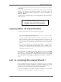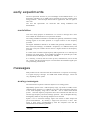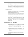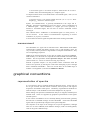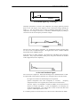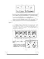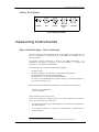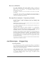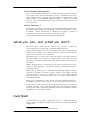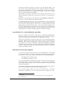
Download Experiment 1

INTRODUCTION TO
MODELLING WITH TIMS
model building ...........................................................................2
why have patching diagrams ? ............................................................... 2
organization of experiments .......................................................3
who is running this experiment ? ................................................3
early experiments.......................................................................4
modulation ........................................................................................... . 4
messages ...................................................................................4
analog messages .................................................................................... 4
digital messages..................................................................................... 5
bandwidths and spectra..............................................................5
measurement ........................................................................................ . 6
graphical conventions ................................................................6
representation of spectra ........................................................................ 6
filters .................................................................................................... . 8
other functions ...................................................................................... . 9
measuring instruments ...............................................................9
the oscilloscope - time domain ............................................................... 9
the rms voltmeter ................................................................................. 10
the spectrum analyser - frequency domain............................................ 10
oscilloscope - triggering...........................................................10
what you see, and what you don`t ............................................11
overload ..................................................................................11
overload of a narrowband system ......................................................... 12
the two-tone test signal ........................................................................ 12
Fourier series and bandwidth estimation...................................13
multipliers and modulators .......................................................13
multipliers ........................................................................................... 13
modulators.......................................................................................... . 14
envelopes ................................................................................15
extremes ..................................................................................15
analog or digital ? ....................................................................15
SIN or COS ? ..........................................................................16
the ADDER - G and g ...........................................................16
abbreviations ...........................................................................17
list of symbols..........................................................................18
Copyright © Emona Instruments Pty Ltd
A1-01-rev 2.1 - 1
INTRODUCTION TO
MODELLING WITH TIMS
model building
With TIMS you will be building models. These models will most often be
hardware realizations of the block diagrams you see in a text book, or have
designed yourself.
They will also be representations of equations, which
themselves can be depicted in block diagram form.
Whatever the origin of the model, it can be patched up in a very short time. The
next step is to adjust the model to perform as expected. It is perfectly true that
you might, on occasions, be experimenting, or just ‘doodling’, not knowing what
to expect. But in most cases your goal will be quite clear, and this is where a
systematic approach is recommended.
If you follow the steps detailed in the first few experiments you will find that the
models are adjusted in a systematic manner, so that each desired result is
obtained via a complete understanding of the purpose and aim of the
intermediate steps leading up to it.
why have patching diagrams ?
Many of the analog experiments, and all of the digital experiments, display
patching diagrams.
These give all details of the interconnections between
modules, to implement a model of the system under investigation.
It is not expected that a glance at the patching diagram
will reveal the nature of the system being modelled.
The patching diagram is presented as firm evidence that a model of the system
can be created with TIMS.
The functional purpose of the system is revealed through the
block diagram which precedes the patching diagram.
A1-01 - 2
Copyright © Emona Instruments Pty Ltd
Introduction to modelling with TIMS
It is the block diagram which you should study to gain insight into the workings
of the system.
If you fully understand the block diagram you should not need the patching
diagram, except perhaps to confirm which modules are required for particular
operations, and particular details of functionality. These is available in the
TIMS User Manual.
You may need an occasional glance at the patching diagram for confirmation of
a particular point.
Try to avoid patching up ‘mechanically’,
according to the patching diagram, without
thought to what you are trying to achieve.
organization of experiments
Each of the experiments in this Text is divided into three parts.
1. The first part is generally titled PREPARATION. This part should be studied
before the accompanying laboratory session.
2. The second part describes the experiment proper. Its title will vary. You will
find the experiment a much more satisfying experience if you arrive at the
laboratory well prepared, rather than having to waste time finding out what
has to be done at the last moment. Thus read this part before the laboratory
session.
3. The third part consists of TUTORIAL QUESTIONS. Generally these
questions will be answered after the experimental work is completed, but it is
a good idea to read them before the laboratory session, in case there are
special measurements to be made.
While performing an experiment you should always have access to the TIMS
user manuals - namely the TIMS User Manual (fawn cover) which contains
information about the modules in the TIMS Basic Set of modules, and the TIMS
Advanced Modules and TIMS Special Applications Modules User Manual (red
cover).
who is running this experiment ?
These experiments and their Tasks are merely suggestions as to how you might
go about carrying out certain investigations. In the final assessment it is you who
are running the experiment, and you must make up your mind as to how you are
going to do it. You can do this best if you read about it beforehand.
If you do not understand a particular instruction, consider what it is you have
been trying to achieve up to that point, and then do it your way.
Copyright © Emona Instruments Pty Ltd
A1-01 - 3
early experiments
The first experiment assumes no prior knowledge of telecommunications - it is
designed to introduce you to TIMS, and to illustrate the previous remarks about
being systematic. The techniques learned will be applied over and over again in
later work.
The next few experiments are concerned with analog modulation and
demodulation.
modulation
One of the many purposes of modulation is to convert a message into a form
more suitable for transmission over a particular medium.
The analog modulation methods to be studied will generally transform the analog
message signal in the audio spectrum to a higher location in the frequency
spectrum.
The digital modulation methods to be studied will generally transform a binary
data stream (the message), at baseband 1 frequencies, to a different format, and
then may or may not translate the new form to a higher location in the frequency
spectrum.
It is much easier to radiate a high frequency (HF) signal than it is a relatively low
frequency (LF) audio signal. In the TIMS environment the particular part of the
spectrum chosen for HF signals is centred at 100 kHz.
It is necessary, of course, that the reverse process, demodulation, can be carried
out - namely, that the message may be recovered from the modulated signal upon
receipt following transmission.
messages
Many models will be concerned with the transmission or reception of a message,
or a signal carrying a message. So TIMS needs suitable messages. These will
vary, depending on the system.
analog messages
The transmission of speech is often the objective in an analog system.
High-fidelity speech covers a wide frequency range, say 50 Hz to 15 kHz, but for
communications purposes it is sufficient to use only those components which lie
in the audio frequency range 300 to 3000 Hz - this is called ‘band limited
speech’. Note that frequency components have been removed from both the low
and the high frequency end of the message spectrum. This is bandpass filtering.
Intelligibility suffers if only the high frequencies are removed.
Speech is not a convenient message signal with which to make simple and
precise measurements. So, initially, a single tone (sine wave) is used. This
signal is more easily accommodated by both the analytical tools and the
instrumentation and measuring facilities.
1 defined later
A1-01 - 4
Copyright © Emona Instruments Pty Ltd
Introduction to modelling with TIMS
The frequency of this tone can be chosen to lie within the range expected in the
speech, and its peak amplitude to match that of the speech. The simple tone can
then be replaced by a two-tone test signal, in which case intermodulation tests
can be carried out 2.
When each modulation or demodulation system has been set up quantitatively
using a single tone as a message (or, preferably with a two-tone test signal), a
final qualitative check can be made by replacing the tone with a speech signal.
The peak amplitude of the speech should be adjusted to match that of the tone.
Both listening tests (in the case of demodulation) and visual examination of the
waveforms can be very informative.
digital messages
The transmission of binary sequences is often the objective of a digital
communication system. Of considerable interest is the degree of success with
which this transmission is achieved. An almost universal method of describing
the quality of transmission is by quoting an error rate 3.
If the sequence is one which can take one of two levels, say 0 and 1, then an error
is recorded if a 0 is received when a 1 was sent, or a 1 received when a 0 was
sent. The bit error rate is measured as the number of errors as a proportion of
total bits sent.
To be able to make such a measurement it is necessary to know the exact nature
of the original message.
For this purpose a known sequence needs to be
transmitted, a copy of which can be made available at the receiver for
comparison purposes. The known sequence needs to have known, and useful,
statistical properties - for example, a ‘random’ sequence. Rather simple
generators can be implemented using shift registers, and these provide sequences
of adjustable lengths. They are known as pseudo-random binary sequence
(PRBS) generators.
TIMS provides you with just such a SEQUENCE
GENERATOR module.
You should refer to a suitable text book for more
information on these.
bandwidths and spectra
Most of the signals you will be examining in the experiments to follow have well
defined bandwidths. That is, in most cases it is possible to state quite clearly that
all of the energy of a signal lies between frequencies f1 and f2 Hz, where f1 < f2.
the absolute bandwidth of such a signal is defined as (f2 - f1) Hz.
It is useful to define the number of octaves a signal occupies.
measure for the above signal is defined as
The octave
octaves = log2(f2 / f1)
Note that the octave measure is a function of the ratio of two frequencies; it says
nothing about their absolute values.
a wideband signal is generally considered to be one which occupies one or
more octaves.
2 the two-tone test signal is introduced in the experiment entitled ‘Amplifier overload’.
3 the corresponding measurement in an analog system would be the signal-to-noise ratio (relatively easy
to measure with instruments), or, if speech is the message, the ‘intelligibility’; not so easy to define, let
alone to measure.
Copyright © Emona Instruments Pty Ltd
A1-01 - 5
a narrowband signal is one which occupies a small fraction of an octave.
Another name, used interchangeably, is a bandpass signal.
An important observation can be made about a narrowband signal; that is, it can
contain no harmonics.
a baseband signal is one which extends from DC (so f1 = 0) to a finite
frequency f2. It is thus a wideband signal.
Speech, for communications, is generally bandlimited to the range 300 to
3000 Hz. It thus has a bandwidth in excess of 3 octaves. This is considered to be
a wideband signal. After modulation, to a higher part of the spectrum, it
becomes a narrowband signal, but note that its absolute bandwidth remains
unchanged.
This reduction from a wideband to a narrowband signal is a linear process; it
can be reversed.
In the context of communications engineering it involves
modulation, or frequency translation.
You will meet all of these signals and phenomena when working with TIMS.
measurement
The bandwidth of a signal can be measured with a SPECTRUM ANALYSER.
Commercially available instruments typically cover a wide frequency range, are
very accurate, and can perform a large number of complex measurements. They
are correspondingly expensive.
TIMS has no spectrum analyser as such, but can model one (with the TIMS320
DSP module), or in the form of a simple WAVE ANALYSER with TIMS analog
modules. See the experiment entitled Spectrum analysis - the WAVE ANALYSER
(within Volume A2 - Further & Advanced Analog Experiments).
Without a spectrum analyser it is still possible to draw conclusions about the
location of a spectrum, by noticing the results when attempting to pass it through
filters of different bandwidths. There are several filters in the TIMS range of
modules. See Appendix A, and also the TIMS User Manual.
graphical conventions
representation of spectra
It is convenient to have a graphical method of depicting spectra. In this work we
do not get involved with the Fourier transform, with its positive and negative
frequencies and double sided spectra. Elementary trigonometrical methods are
used for analysis. Such methods are more than adequate for our purposes.
When dealing with speech the mathematical analysis is dropped, and descriptive
methods used. These are supported by graphical representations of the signals
and their spectra.
In the context of modulation we are constantly dealing with sidebands, generally
derived from a baseband message of finite bandwidth. Such finite bandwidth
signals will be represented by triangles on the spectral diagrams.
The steepness of the slope of the triangle has no special significance, although
when two or more sidebands, from different messages, need to be distinguished,
each can be given a different slope.
A1-01 - 6
Copyright © Emona Instruments Pty Ltd
Introduction to modelling with TIMS
frequency
a baseband signal (eg., a message)
Although speech does not have a DC component, the triangle generally extends
down to zero (the origin) of the frequency scale (rather than being truncated just
before it). For the special case in which a baseband signal does have a DC
component the triangle convention is sometimes modified slightly by adding a
vertical line at the zero-frequency end of the triangle.
a DSBSC
The direction of the slope is important. Its significance becomes obvious when
we wish to draw a modulated signal. The figure above shows a double sideband
suppressed carrier (DSBSC) signal.
Note that there are TWO triangles, representing the individual lower and upper
sidebands. They slope towards the same point; this point indicates the location
of the (suppressed) carrier frequency.
an inverted baseband signal
The orientation is important. If the same message was so modulated that it could
be represented in the frequency spectrum as in the figure above, then this means:
the signal is located in the baseband part of the spectrum
spectral components have been transposed, or inverted;
frequency
components which were originally above others are now below them.
since the signal is at baseband it would be audible (if converted with an
electric to acoustic transducer - a pair of headphones, for example), but
would be unintelligible. You will be able to listen to this and other such
signals in TIMS experiments to come.
It is common practice to use the terms erect and inverted to describe these bands.
Copyright © Emona Instruments Pty Ltd
A1-01 - 7
In the Figure above, a message (a) is frequency translated to become an upper
single sideband (b), and a lower single sideband (c). A three-channel frequency
division multiplexed (FDM) signal is also illustrated (d).
Note that these spectral diagrams do not show any phase information.
Despite all the above, be prepared to accept that these diagrams are used for
purposes of illustration, and different authors use their own variations. For
example, some slope their triangles in the opposite sense to that suggested here.
filters
In a block diagram, there is a simple technique for representing filters. The
frequency spectrum is divided into three bands - low, middle, and high - each
represented by part of a sinewave. If a particular band is blocked, then this is
indicated by an oblique stroke through it. The standard responses are
represented as in the Figure below.
block-diagrammatic representations of filter responses
The filters are, respectively, lowpass,
bandpass, highpass, bandstop, and
allpass.
In the case of lowpass and highpass
responses the diagrams are often further
simplified by the removal of one of the
cancelled sinewaves, the result being as
in the figure opposite.
A1-01 - 8
Copyright © Emona Instruments Pty Ltd
Introduction to modelling with TIMS
other functions
amplify
add
multiply
amplitude
limit
integrate
some analog functions
measuring instruments
the oscilloscope - time domain
The most frequently used measuring facility with TIMS is the oscilloscope. In
fact the vast majority of experiments can be satisfactorily completed with no
other instrument.
Any general purpose oscilloscope is ideal for all TIMS experiments. It is
intended for the display of signals in the time domain 4. It shows their
waveforms - their shapes, and amplitudes
From the display can be obtained information regarding:
waveform shape
waveform frequency - by calculation, using time base information
waveform amplitude - directly from the display
system linearity - by observing waveform distortion
an estimate of the bandwidth of a complex signal; eg, from the sharpness of
the corners of a square wave
When concerned with amplitude information it is customary to record either:
the peak-to-peak amplitude
the peak amplitude
of the waveform visible on the screen.
Unless the waveform is a simple sinewave it is always important to record the
shape of the waveform also; this can be:
1. as a sketch (with time scale), and annotation to show clearly what amplitude
has been measured.
2. as an analytic expression, in which case the parameter recorded must be
clearly specified.
4 but with adaptive circuitry it can be modified to display frequency-domain information
Copyright © Emona Instruments Pty Ltd
A1-01 - 9
the rms voltmeter
The TIMS WIDEBAND TRUE RMS METER module is essential for
measurements concerning power, except perhaps for the simple case when the
signal is one or two sinewaves. It is particularly important when the
measurement involves noise.
Its bandwidth is adequate for all of the signals you will meet in the TIMS
environment.
An experiment which introduces the WIDEBAND TRUE RMS METER, is
entitled Power measurements. Although it appears at the end of this Volume, it
could well be attempted at almost any time.
the spectrum analyser - frequency domain
The identification of the spectral composition of a signal - its components in the
frequency domain - plays an important part when learning about
communications.
Unfortunately, instruments for displaying spectra tend to be far more expensive
than the general purpose oscilloscope.
It is possible to identify and measure the individual spectral components of a
signal using TIMS modules.
Instruments which identify the spectral components on a component-bycomponent basis are generally called wave analysers.
A model of such an
instrument is examined in the experiment entitled Spectrum analysis - the WAVE
ANALYSER in Volume A2 - Further & Advanced Analog Experiments.
Instruments which identify the spectral components of a signal and display the
spectrum are generally called spectrum analysers. These instruments tend to be
more expensive than wave analysers. Something more sophisticated is required
for their modelling, but this is still possible with TIMS, using the digital signals
processing (DSP) facilities - the TIMS320 module can be programmed to provide
spectrum analysis facilities.
Alternatively the distributors of TIMS can recommend other affordable methods,
compatible with the TIMS environment.
oscilloscope - triggering
synchronization
As is usually the case, to achieve ‘text book like’ displays, it is important to
choose an appropriate signal for oscilloscope triggering. This trigger signal is
almost never the signal being observed ! The recognition of this point is an
important step in achieving stable displays.
This chosen triggering signal should be connected directly to the oscilloscope
sweep synchronizing circuitry. Access to this circuitry of the oscilloscope is
available via an input socket other than the vertical deflection amplifier input(s).
It is typically labelled ‘ext. trig’ (external trigger), ‘ext. synch’ (external
synchronization), or similar.
A1-01 - 10
Copyright © Emona Instruments Pty Ltd
Introduction to modelling with TIMS
sub-multiple frequencies
If two or more periodic waveforms are involved, they will only remain stationary
with respect to each other if the frequency of one is a sub-multiple of the other.
This is seldom the case in practice, but can be made so in the laboratory. Thus
TIMS provides, at the MASTER SIGNALS module, a signal of 2.083 kHz
(which is 1/48 of the 100 kHz system clock), and another at 8.333 kHz (1/12 of
the system clock).
which channel ?
Much time can be saved if a consistent use of the SCOPE SELECTOR is made.
This enables quick changes from one display to another with the flip of a switch.
In addition, channel identification is simplified if the habit is adopted of
consistently locating the trace for CH1 above the trace for CH2.
Colour coded patching leads can also speed trace identification.
what you see, and what you don`t
Instructions such as ‘adjust the phase until there is no output’, or ‘remove the
unwanted signal with a suitable filter’ will be met from time to time.
These instructions seldom result in the amplitude of the signal in question being
reduced to zero. Instead, what is generally meant is ‘reduce the amplitude of the
signal until it is no longer of any significance’.
Significance here is a relative term, made with respect to the system signal-tonoise ratio (SNR). All systems have a background noise level (noise threshold,
noise floor), and signals (wanted) within these systems must over-ride this noise
(unwanted).
TIMS is designed to have a ‘working level’, the TIMS ANALOG REFERENCE LEVEL,
of about 4 volts peak-to-peak. The system noise level is claimed to be at least
100 times below this 5.
When using an oscilloscope as a measuring instrument with TIMS, the vertical
sensitivity is typically set to about 1 volt/cm. Signals at the reference level fit
nicely on the screen. If they are too small it is wise to increase them if possible
(and appropriate), to over-ride the system noise; or if larger to reduce them, to
avoid system overload.
When they are attenuated by a factor of 100, and if the oscilloscope sensitivity is
not changed, they appear to be ‘reduced to zero’; and in relative terms this is so.
If the sensitivity of the oscilloscope is increased by 100, however, the screen will
no longer be empty. There will be the system noise, and perhaps the signal of
interest is still visible. Engineering judgement must then be exercised to evaluate
the significance of the signals remaining.
overload
If wanted signal levels within a system fall ‘too low’ in amplitude, then the
signal-to-noise ratio (SNR) will suffer, since internal circuit noise is independent
of signal level.
5 TIMS claims a system signal-to-noise ratio of better than 40 dB
Copyright © Emona Instruments Pty Ltd
A1-01 - 11
If signal levels within a system rise ‘too high’, then the SNR will suffer, since
the circuitry will overload, and generate extra, unwanted, distortion components;
these distortion components are signal level dependent. In this case the noise is
derived from distortion of the signal, and the degree of distortion is usually
quoted as signal-to-distortion ratio (SDR).
Thus analog circuit design includes the need to maintain signal levels at a predefined working level, being ‘not to high’ and ‘not too low’, to avoid these two
extremes.
These factors are examined in the experiment entitled Amplifier overload within
Volume A2 - Further & Advanced Analog Experiments.
The TIMS working signal level, or TIMS ANALOG REFERENCE LEVEL, has been set
at 4 volts peak-to-peak. Modules will generally run into non-linear operation
when this level is exceeded by say a factor of two. The background noise of the
TIMS system is held below about 10 mV - this is a fairly loose statement, since
this level is dependent upon the bandwidth over which the noise is measured, and
the model being examined at the time. A general statement would be to say that
TIMS endeavours to maintain a SNR of better than 40 dB for all models.
overload of a narrowband system
Suppose a channel is narrowband. This means it is deliberately bandlimited so
that it passes signals in a narrow (typically much less than an octave 6) frequency
range only. There are many such circuits in a communications system.
If this system overloads on a single tone input, there will be unwanted harmonics
generated. But these will not pass to the output, and so the overload may go
unnoticed. With a more complex input - say two or more tones, or a speechrelated signal - there will be, in addition, unwanted intermodulation components
generated. Many of these will pass via the system, thus revealing the existence of
overload. In fact, the two-tone test signal should always be used in a narrowband
system to investigate overload.
the two-tone test signal
A two-tone test signal consists of two sine waves added together ! As discussed
in the previous section, it is a very useful signal for testing systems, especially
those which are of narrow-bandwidth. The properties of the signal depend upon:
the frequency ratio of the two tones.
the amplitude ratio of the two tones.
For testing narrowband communication systems the two tones are typically of
near-equal frequency, and of identical amplitude. A special property of this form
of the signal is that its shape, as seen in the time domain, is very well defined
and easily recognisable 7.
After having completed the early experiments you will recognise this shape as
that of the double sideband suppressed carrier (DSBSC) signal.
If the system through which this signal is transmitted has a non-linear
transmission characteristic, then this will generate extra components. The
6 defined above
7 the assumption being that the oscilloscope is set to sweep across the screen over a few periods of the
difference frequency.
A1-01 - 12
Copyright © Emona Instruments Pty Ltd
Introduction to modelling with TIMS
presence of even small amounts of these components is revealed by a change of
shape of the test signal.
Fourier series and bandwidth
estimation
Fourier series analysis of periodic signals reveals that:
it is possible, by studying the symmetry of a signal, to predict the presence or
absence of a DC component.
if a signal is other than sinusoidal, it will contain more than one harmonic
component of significance.
if a signal has sharp discontinuities, it is likely to contain many harmonic
components of significance
some special symmetries result in all (or nearly all) of the ODD (or EVEN)
harmonics being absent.
With these observations, and more, it is generally easy to make an engineering
estimate of the bandwidth of a periodic signal.
multipliers and modulators
The modulation process requires multiplication.
seldom found in communications equipment.
MODULATOR is used.
But a pure MULTIPLIER is
Instead, a device called a
In the TIMS system we generally use a MULTIPLIER, rather than a
MODULATOR, when multiplication is called for, so as not to become diverted
by the side effects and restrictions imposed by the latter.
In commercial practice, however, the purpose-designed MODULATOR is
generally far superior to the unnecessarily versatile MULTIPLIER.
multipliers
An ideal multiplier performs as a multiplier should ! That is, if the two timedomain functions x(t) and y(t) are multiplied together, then we expect the result
to be x(t).y(t), no more and no less, and no matter what the nature of these two
functions. These devices are called four quadrant multipliers.
There are practical multipliers which approach this ideal, with one or two
engineering qualifications. Firstly, there is always a restriction on the bandwidth
of the signals x(t) and y(t).
There will inevitably be extra (unwanted) terms in the output (noise, and
particularly distortion products) due to practical imperfections.
Provided these unwanted terms can be considered ‘insignificant’, with respect to
the magnitude of the wanted terms, then the multiplier is said to be ‘ideal’. In
Copyright © Emona Instruments Pty Ltd
A1-01 - 13
the TIMS environment this means they are at least 40 dB below the TIMS ANALOG
REFERENCE LEVEL 8.
Such a multiplier is even said to be linear. That is, from an engineering point of
view, it is performing as expected.
In the mathematical sense it is not linear, since the mathematical definition of a
linear circuit includes the requirement that no new frequency components are
generated when it performs its normal function.
But, as will be seen,
multiplication always generates new frequency components.
DC off-sets
One of the problems associated with analog circuit design is minimization of
unwanted DC off-sets. If the signals to be processed have no DC component
(such as in an audio system) then stages can be AC coupled, and the problem is
overcome. In the TIMS environment module bandwidths must extend to DC, to
cope with all possible conditions; although more often than not signals have no
intentional DC component.
In a complex model DC offsets can accumulate - but in most cases they can be
recognised as such, and accounted for appropriately. There is one situation,
however, where they can cause much more serious problems by generating new
components - and that is when multiplication is involved.
With a MULTIPLIER the presence of an unintentional DC component at one
input will produce new components at the output. Specifically, each component
at the other input will be multiplied by this DC component - a constant - and so
a scaled version will appear at the output 9.
To overcome this problem there is an option for AC coupling in the
MULTIPLIER module. It is suggested that the DC mode be chosen only when
the signals to be processed actually have DC components; otherwise use AC
coupling.
modulators
In communications practice the circuitry used for the purpose of performing the
multiplying function is not always ideal in the four quadrant multiplier sense;
such circuits are generally called modulators.
Modulators generate the wanted sum or difference products but in many cases the
input signals will also be found in the output, along with other unwanted
components at significant levels. Filters are used to remove these unwanted
components from the output (alternatively there are ‘balanced’ modulators.
These have managed to eliminate either one or both of the original signals from
the output).
These modulators are restricted in other senses as well. It is allowed that one of
the inputs can be complex (ie., two or more components) but the other can only
be a single frequency component (or appear so to be - as in the switching
modulator). This restriction is of no disadvantage, since the vast majority of
modulators are required to multiply a complex signal by a single-component
carrier.
Accepting restrictions in some areas generally results in superior performance in
others, so that in practice it is the switching modulator, rather than the idealized
8 defined under ‘what you see and what you don`t’
9 this is the basis of a voltage controlled amplifier - VCA
A1-01 - 14
Copyright © Emona Instruments Pty Ltd
Introduction to modelling with TIMS
four quadrant multiplier, which finds universal use in communications
electronics.
Despite the above, TIMS uses the four quadrant multiplier in most applications
where a modulator might be used in practice. This is made possible by the
relatively low frequency of operation, and modest linearity requirements
envelopes
Every narrowband signal has an envelope, and you probably have an idea of what
this means.
Envelopes will be examined first in the experiment entitled DSB generation in
this Volume.
They will be defined and further investigated in the experiments entitled
Envelopes within this Volume, and Envelope recovery within Volume A2 Further & Advanced Analog Experiments.
extremes
Except for a possible frequency scaling effect, most experiments with TIMS will
involve realistic models of the systems they are emulating.
Thus message
frequencies will be ‘low’, and carrier frequencies ‘high’. But these conditions
need not be maintained. TIMS is a very flexible environment.
It is always a rewarding intellectual exercise to
imagine what would happen if one or more of
the ‘normal’ conditions was changed severely 10.
It is then even more rewarding to confirm our imaginings by actually modelling
these unusual conditions. TIMS is sufficiently flexible to enable this to be done
in most cases.
For example: it is frequently stated, for such-and-such a requirement to be
satisfied, that it is necessary that ‘x1 >> x2’. Quite often x1 and x2 are
frequencies - say a carrier and a message frequency; or they could be amplitudes.
You are strongly encouraged to expand your horizons by questioning the reasons
for specifying the conditions, or restrictions, within a model, and to consider, and
then examine, the possibilities when they are ignored.
analog or digital ?
What is the difference between a digital signal and an analog signal ?
Sometimes this is not clear or obvious.
10 for an entertaining and enlightening look at the effects of major changes to one or more of the physical
constants, see G. Gamow; Mr Tompkins in Wonderland published in 1940, or easier Mr. Tompkins in
Paperback, Cambridge University Press, 1965.
Copyright © Emona Instruments Pty Ltd
A1-01 - 15
In TIMS digital signals are generally thought of as those being compatible with
the TTL standards. Thus their amplitudes lie in the range 0 to +5 volts. They
come from, and are processed by, modules having RED output and input sockets.
It is sometimes necessary, however, to use an analog filter to bandlimit these
signals. But their large DC offsets would overload most analog modules, . Some
digital modules (eg, the SEQUENCE GENERATOR) have anticipated this, and
provide an analog as well as a digital (TTL) output. This analog output comes
from a YELLOW socket, and is a TTL signal with the DC component removed
(ie, DC shifted).
SIN or COS ?
Single frequency signals are generally referred to as sinusoids, yet when
manipulating them trigonometrically are often written as cosines. How do we
obtain cos t from a sinusoidal oscillator !
There is no difference in the shape of a sinusoid and a cosinusoid, as observed
with an oscilloscope. A sinusoidal oscillator can just as easily be used to provide
a cosinusoid. What we call the signal (sin or cos) will depend upon the time
reference chosen.
Remember that cos t = sin( t + /2)
Often the time reference is of little significance, and so we choose sin or cos, in
any analysis, as is convenient.
the ADDER - G and g
Refer to the TIMS User Manual for a description of the ADDER module. Notice
it has two input sockets, labelled ‘A’ and ‘B’.
In many experiments an ADDER is used to make a linear sum of two signals a(t)
and b(t), of amplitudes A and B respectively, connected to the inputs A and B
respectively. The proportions of these signals which appear at the ADDER
output are controlled by the front panel gain controls G and g.
The amplitudes A and B of the two input signals are seldom measured, nor the
magnitudes G and g of the adjustable gains.
Instead it is the magnitudes GA and gB which are of more interest, and these are
measured directly at the ADDER output. The measurement of GA is made when
the patch lead for input B is removed; and that of gB is measured when the
patch lead for input A is removed.
When referring to the two inputs in this text it would be formally correct to name
them as ‘the input A’ and ‘the input B’. This is seldom done. Instead, they are
generally referred to as ‘the input G’ and ‘the input g’ respectively (or sometimes
just G and g). This should never cause any misunderstanding. If it does, then it
is up to you, as the experimenter, to make an intelligent interpretation.
A1-01 - 16
Copyright © Emona Instruments Pty Ltd
Introduction to modelling with TIMS
abbreviations
This list is not exhaustive. It includes only those abbreviations used in this Text.
abbreviation
AM
ASK
BPSK
CDMA
CRO
dB
DPCM
DPSK
DSB
DSBSC
DSSS
DUT
ext. synch.
ext. trig.
FM
FSK
FSD
IP
ISB
ISI
LSB
MSB
NBFM
OOK
PAM
PCM
PDM
PM
PPM
PRK
PSK
PWM
SDR
SNR
SSB
SSBSC
SSR
TDM
THD
VCA
WBFM
Copyright © Emona Instruments Pty Ltd
meaning
amplitude modulation
amplitude shift keying (also called OOK)
binary phase shift keying
code division multiple access
cathode ray oscilloscope
decibel
differential pulse code modulation
differential phase shift keying
double sideband (in this text synonymous with DSBSC)
double sideband suppressed carrier
direct sequence spread spectrum
device under test
external synchronization (of oscilloscope). ‘ext. trig.’ preferred
external trigger (of an oscilloscope)
frequency modulation
frequency shift keying
full scale deflection (of a meter, for example)
intermodulation product
independent sideband
intersymbol interference
analog: lower sideband digital: least significant bit
most significant bit
narrow band frequency modulation
on-off keying (also called ASK)
pulse amplitude modulation
pulse code modulation
pulse duration modulation (see PWM)
phase modulation
pulse position modulation
phase reversal keying (also called PSK)
phase shift keying (also called PRK - see BPSK)
pulse width modulation (see PDM)
signal-to-distortion ratio
signal-to-noise ratio
single sideband (in this text is synonymous with SSBSC)
single sideband suppressed carrier
sideband suppression ratio
time division multiplex
total harmonic distortion
voltage controlled amplifier
wide band frequency modulation
A1-01 - 17
list of symbols
The following symbols are used throughout the text, and have the following
meanings
a(t)
a time varying amplitude
, , ,
phase angles
deviation, in context of PM and FM
f
a small frequency increment
peak phase deviation
t a small time interval
(t)
m
a time varying phase
in the context of envelope modulation, the depth of modulation
a low frequency (rad/s); typically that of a message ( << ).
a high frequency (rad/s); typically that of a carrier ( >> )
y(t)
A1-01 - 18
a time varying function
Copyright © Emona Instruments Pty Ltd