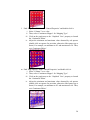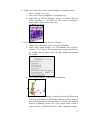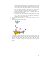
1
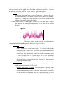
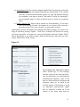
AutoSOME User Manual
February 16, 2014
Written by Aaron M. Newman, Ph.D.
Institute for Stem Cell Biology and Regenerative Medicine
Stanford University
Table of Contents
Introduction ...................................................................................................................................... 1
System Requirements ....................................................................................................................... 1
Installing and Running the AutoSOME GUI ................................................................................... 1
Using AutoSOME ............................................................................................................................ 2
Input Format ................................................................................................................................. 2
Missing Values ............................................................................................................................. 3
AutoSOME GUI ........................................................................................................................... 3
Load (and Filter) Input ............................................................................................................. 3
Input Adjustment ...................................................................................................................... 6
Basic Fields .............................................................................................................................. 7
Advanced Fields ....................................................................................................................... 8
Fuzzy Cluster Networks .................................................................................................................. 8
Memory ........................................................................................................................................... 8
Algorithm Settings .......................................................................................................................... 8
Self-Organizing Map (SOM) .................................................................................................. 8
Cartogram ............................................................................................................................... 9
Running AutoSOME ................................................................................................................ 9
Output ..................................................................................................................................... 10
Output Files ................................................................................................................................... 10
Cluster tree .................................................................................................................................... 10
Heat maps ...................................................................................................................................... 11
Signal plots .................................................................................................................................... 12
View>settings>Image Settings ...................................................................................................... 12
View>settings>scale using entire data set ..................................................................................... 13
Search ............................................................................................................................................ 14
Saving data .................................................................................................................................... 14
Files written to disk ....................................................................................................................... 14
Opening previous clustering results .............................................................................................. 15
Reset .............................................................................................................................................. 15
Enhanced GUI vs. Basic GUI ........................................................................................................ 15
AutoSOME Command Line Version ......................................................................................... 16
Creating Fuzzy Cluster Networks .................................................................................................. 18
References ...................................................................................................................................... 23
Introduction
AutoSOME is a powerful unsupervised computational method for identifying discrete
and fuzzy clusters of diverse geometries from potentially large, multi-dimensional, data
sets without prior knowledge of cluster number or structure [Newman and Cooper, 2010].
We have implemented the AutoSOME method as a Graphical User Interface (GUI) and
command line tool to facilitate its use by the academic research community. Below,
instructions are provided for using both versions of AutoSOME, and a protocol is given
for generating AutoSOME fuzzy cluster networks in Cytoscape [Shannon et al., 2005].
Refer to the AutoSOME website for tutorials, software, and FAQ
[http://jimcooperlab.mcdb.ucsb.edu/autosome].
System Requirements
AutoSOME is coded in Java to promote platform independence. To launch the GUI from
the AutoSOME website [http://jimcooperlab.mcdb.ucsb.edu/autosome], Java Web Start
technology needs to be installed on your computer along with Java Standard Edition 1.6,
both of which are freely available at http://java.sun.com. The command line version of
AutoSOME will run in JAVA 1.5 and perhaps earlier versions. In general, the more
memory and processors available, the better the performance of AutoSOME. Without
user intervention, both the GUI and command line versions will greedily use all available
CPUs. For 32-bit Windows systems, the maximum amount of memory that can be
allocated to AutoSOME is about 1.6 GB, while 64-bit operating systems with 64-bit Java
can allocate up to ~30 GB of memory. Microarray data sets like the HG U133 Plus 2.0
Affymetrix chipset (>54k probes) with dozens of samples can be run with 1.6 GB RAM.
The ‘Java Web Start’ launch button on the ‘AutoSOME Web Portal’ homepage
will automatically allocate up to 1 GB of RAM. To run AutoSOME with more or
less memory, download the .jar file from:
http://jimcooperlab.mcdb.ucsb.edu/autosome/downloads.
Installing and Running the AutoSOME GUI
Download AutoSOME from the website, and then unzip all contents of the downloaded
archive into the same directory. Using your system console, navigate to the directory
where you installed AutoSOME, and type:
java –Xmx1600m –Xms1600m –jar autosome_vXXXXXX.jar
XXXXXX = the GUI version you downloaded (each version is named by the date of
compilation, e.g. 120109). The -Xmx,-Xms arguments allocate additional memory to the
1
Java Virtual Machine necessary for running large data sets. Allocate more or less
memory as needed for your input data set, parameters, and machine architecture. Also,
AutoSOME has not been internationalized. If it is behaving oddly, try adding the
following JVM argument ‘-Duser.language=en’.
For instructions on how to use the AutoSOME command line interface, see AutoSOME
Command Line Version below.
Using AutoSOME
Input Format
AutoSOME accepts three kinds of numerical input files.
Standard format: The input file is a table of numerical values with optional column
labels (row 1) and mandatory row labels (column 1). If column labels are specified,
column 1 also needs a label in row 1. All entries must be tab, comma, or space delimited.
Input data can be easily formatted using Microsoft Excel. See Table 1 below for an
example.
Table 1
Probe
hESC-1
hESC-2
hESC-3
hESC-4
iPSC-1
iPSC-2
iPSC-3
212853_at
212854_x_at
212855_at
212856_at
212857_x_at
8.221449
8.523748
10.64296
8.936721
6.195244
8.297634
8.706556
10.4093
9.218977
5.929077
7.694108
8.044123
10.60148
9.109346
4.432911
8.215596
8.992252
11.03563
8.425392
6.764105
10.1284
8.87927
12.08599
8.431269
4.344787
10.25488
8.974617
11.91321
8.418733
4.786857
10.21546
9.083473
12.04592
8.450901
4.953329
Microarray formats:
1) Gene Expression Omnibus (GEO) Series Matrix. This format contains all
chipset expression data as well as user-supplied annotation in a spreadsheet style.
AutoSOME can automatically extract expression information content and column
names from a raw series matrix file. This allows for rapid analysis of any GEO
data set by simply downloading the archive containing the series matrix text file,
unzipping it, and loading it into AutoSOME.
2) PCL = Pre CLuster format used for the Cluster software [Eisen et al. (1998)
PNAS 95:14863].
For an example, see http://puma.princeton.edu/help/formats.shtml#pcl or the
Cluster/TreeView User Manual. The first two columns are reserved for gene
annotation (column 1 = row identifiers, column 2 = gene names or annotation).
Column 3 is optional, is called GWEIGHT, and specifies how to weigh each gene
2
when computing gene-gene similarity. This column is read by AutoSOME, but is
ignored since AutoSOME does not cluster genes using a similarity matrix. Row 1
is mandatory and is used to provide column names including names of each array
(e.g. ID, NAME, GWEIGHT, array1, array2, …). Row 2 is optional, is called
EWEIGHT, and specifies how each array is weighed when computing array-array
similarity. In contrast to GWEIGHT, AutoSOME will use EWEIGHT when
constructing a distance matrix for transcriptome clustering (fuzzy cluster
networks option).
Missing Values
There are two strategies implemented in AutoSOME for handling missing values (blank
space, ‘?’, or ‘NA’).
1) Replace missing values with median of columns (or rows).
2) Replace missing values with mean of columns (or rows).
Go to File>Settings to launch a window that will allow you to specify which of these two
techniques to use.
AutoSOME GUI
The AutoSOME GUI is launched using Java Web Start from your browser or via the
command line, and is used to run AutoSOME as well as to browse and generate
publication quality visualizations of the cluster output (Figure 1).
Figure 1
Load (and Filter) Input
To begin, launch a file browser by either pressing the large ‘INPUT’ button in the
‘AutoSOME Steps’ panel on the top left, or by clicking the browse button adjacent to the
input file text box in the ‘Input and Output’ section (Figure 1). A file browser will appear.
For standard input (see Input Format above), simply find your file and open it. For
3
microarray input, optional data formats are shown at the top of the file browser (see
Figure 2). Select the appropriate file format for your microarray data set and load the file.
Figure 2
Once loaded, you will be asked whether you want to filter your input data set (Figure 3).
Figure 3
If you choose ‘yes’ you will be redirected to a ‘Filter Data’ window (Figure 4 below).
This window provides two simple data filtration options:
i)
Remove rows with fold change less than X. The fold change is calculated
by the difference between the minimum and maximum values for each
row. All rows with fold change <X will be removed. Importantly, if your
data are already log2 scaled, make sure you select the corresponding
checkbox.
ii)
Remove rows with mean value below Y. The mean µ of each row is
calculated, and the row is removed if µ <Y.
After specifying filtration options, press ‘Apply’ to preview the filtered data, and if you
approve, press ‘Accept’.
4
Figure 4
Figure 5
After your input file has loaded, the
number of rows and columns will be
displayed in the ‘Input Data’ panel on
the left side of the GUI (see Figure 5).
The maximum and minimum values
over the entire data set are also provided.
When finished clustering, this table will
dynamically update based on the
contents of selected clusters in the
cluster tree (see Output below).
5
Input Adjustment
AutoSOME implements several input normalization methods in addition to log2 scaling.
For an excellent overview of these techniques, see the manual to the Cluster software
available at http://rana.lbl.gov/manuals/ClusterTreeView.pdf [Eisen et al., 1998]. Press
the ‘Show’ button to the right of the ‘Input Adjustment’ label to access input scaling and
normalization options (see Figure 6 below). All input adjustment operations are
performed in the order listed in the GUI, from top to bottom. In brief:
i) Log2 Scaling: Logarithmic scaling is routinely used for microarray data sets to
amplify small fold changes in gene expression, and is completely reversible.
We recommend applying log2 scaling in cases where expression values span
several orders of magnitude. All other implemented input adjustment methods
irreversibly change the input to make it more suitable for analysis.
ii) Unit variance: forces all columns to have zero mean and a standard deviation of
one, and is commonly used when there is no a priori reason to treat any
column differently from any other.
iii) Range [0,x]: Alternatively, data in all columns can be normalized to share lowest
and highest values (0,x) by specifying an upper bound x.
iv) Median Center Rows/Arrays: For microarray analysis, centering each gene (row)
and/or array (column) by subtracting the median value of the row/column
eliminates amplitude shifts to cluster distinct expression patterns rather than
overall transcript levels. We recommend applying median centering to genes
before co-expression clustering (clustering rows).
v) Sum of Squares=1 Rows/Arrays: This normalization procedure smoothes the data
set by forcing the sum of squares of all expression values to equal 1 for each
row/column in the data set. The impact of this method on cluster identification
can be significant and tends to result in the detection of larger clusters trailing
off into genes with minimal differential expression (after clustering, the signal
to noise ratio can be boosted by using the confidence filter; see Output below)
As an example, to run AutoSOME co-expression analysis, one may apply log2 scaling,
unit variance normalization, and median-centering of genes (and/or arrays). To run
AutoSOME transcriptome clustering (fuzzy cluster networks, see tutorial below), it is
generally recommended to apply unit variance normalization to your data set. Other
normalization settings may also be desirable. Input can also be adjusted using Microsoft
Excel or the Cluster software [Eisen et al., 1998] and then imported into AutoSOME.
6
Figure 6
Basic Fields
Press the ‘Show’ button to expand the ‘Basic Fields’ section (see Figure 6).
i) Cluster Analysis: Switch among clustering rows (e.g. genes), columns (e.g.
experiments), or both rows and columns in a single step.
ii) Running Mode: This parameter alters advanced AutoSOME algorithm settings to
switch among ‘Precision’, ‘Normal’, and ‘Speed’ modes of operation. ‘Precision’
takes longer, but provides greater training of the SOM node lattice (2X1000
iterations) and greater resolution for density-equalization of the SOM error surface
(64X64). For enhanced performance, and especially for first-pass exploratory cluster
analysis, choose ‘Speed’ for less SOM iterations (2X250) and less resolution for
density-equalization (16X16). ‘Normal’ provides a compromise between the other
two settings (2X500 SOM iterations and 32X32 cartogram resolution). In our
experiments, ‘Normal’ works quite well, and in fact, often yields comparable results
to ‘Precision’. Choose ‘Speed’ for a first-pass exploratory analysis.
iii) No. Ensemble Runs: The default of 50 ensemble iterations should be sufficient to
begin investigating the cluster structure of most data sets. Although in practice,
AutoSOME clustering results can be quite stable with ~50 ensemble iterations (and
even as little as 20), for final clustering results, it is recommended to increase this
number to at least 100.
iv) P-value Threshold: AutoSOME has been extensively benchmarked on a highly
diverse array of clustering problems using a P-value cutoff of 0.1. Reduce the p-value
threshold to identify tighter clusters.
7
v) No. CPUs: To liberate processor resources, decrease ‘No. CPUs’. AutoSOME
running time will decrease approximately linearly with respect to increasing number
of dedicated CPUs.
Advanced Fields
Fuzzy Cluster Networks. When clustering columns (i.e. ‘Cluster Analysis’ in Basic Fields
is set to ‘columns’ or ‘both’), the ‘Fuzzy Cluster Networks’ window will be automatically
enabled (see Figure 6). In this window, you can pick one of three distance metrics for
calculating the input distance matrix (Euclidean, Pearson’s and Uncentered correlation).
Euclidean distance is selected by default due to good results obtained from empirical
testing. See the review by D’haeseleer (2005) for descriptions of Euclidean, Pearson’s
and Uncentered correlation distance metrics. In brief, Euclidean distance is sensitive to
amplitude shifts while Pearson’s correlation is not. Experiment with these metrics to get a
feel for how they work. If smoothing out the distance matrix is desired, ‘Unit Variance
Normalize’ can be selected to normalize the distance matrix columns to unit variance.
When finished clustering, AutoSOME will automatically generate additional output files
for building fuzzy cluster networks in Cytoscape (see Fuzzy Cluster Networks below).
Memory. Write Intermediate Runs to Disk: If AutoSOME crashes (or seems to hang for a
long period of time), then ‘Write Ensemble Runs to Disk’ should be selected (see Figure
6) as an out of memory error is likely. This may be necessary on systems with
insufficient RAM for large data sets and many ensemble runs (e.g. 45k probes, 100
samples, and 2000 ensemble runs). Overall running time will be slower due to reading
and writing to disk. Files will be written to a temporary folder in the output directory.
Also, try reducing the number of CPUs to free up memory.
Algorithm Settings. Press the ‘Show’ button to expand the ‘Algorithm Settings’ section
(see Figure 6). The GUI permits modification of the most critical algorithm parameters.
For access to all algorithm parameters, use the command line version of AutoSOME.
Self-Organizing Map (SOM).
i) Maximum Grid Length: The maximum number of nodes for the x/y length of the
SOM node lattice.
ii) Minimum Grid Length: The minimum number of nodes for the x/y length of the
SOM node grid.
In general increase ‘Maximum Grid Length’ to provide greater resolution for
cluster separation in the SOM, and to increase the number of possible clusters.
Increase ‘Minimum Grid Length’ to force AutoSOME to use an SOM lattice with
8
specific minimum dimensions. Set both parameters to the same value to disable
automatic adjustment of grid length by the algorithm. The SOM grid length is set,
by default, between 5 and 30, providing sufficient cluster resolving power for
most clustering problems. If a data set with at least 5,000 rows is imported (e.g.
whole-genome microarray), the maximum grid length will be automatically set to
20 for more efficient running time.
iii) Training Iterations: The number of iterations for training the SOM node lattice.
The value of this parameter dictates the number of iterations for each of two
phases, coarse-grained followed by fine-grained training. This value can be
toggled between ‘1000’ iterations for precision (used during benchmarking in
Newman and Cooper, 2010), ‘500’ iterations for normal, and ‘250’ iterations
for speed.
iv) Use Square Topology: Select this checkbox to use a square-shaped node lattice
rather than a circular node lattice (default). Benchmarking results indicate
both topologies yield comparable results. See the Manuscript for more details.
Cartogram. Resolution: The density-equalizing cartogram algorithm requires an input
array with dimensions that are a power of two. Although all benchmarking tests
were conducted using an array size of 64X64, greater resolutions may yield more
accurate density-equalization (especially when the SOM dimensions are large).
On the other hand, going from 64X64 to 32X32 may increase running time
dramatically (up to ~4X), and is sufficient for accurate clustering results in many
cases (especially when the SOM dimensions are less than 30X30).
Running AutoSOME
After the input file and parameters are specified, execute AutoSOME clustering by
pressing the green ‘RUN’ button in the ‘AutoSOME Steps’ panel (see Figure 1). Progress
is shown in the lower left corner of the GUI and elapsed time is displayed (see Figure 7).
When finished, the GUI will automatically be redirected to the output panel for browsing
the cluster output. The input and output panels can be toggled back and forth using the
tabs or the ‘INPUT’ and ‘OUTPUT’ buttons in the control panel.
Figure 7
9
Output
Output Files. The ‘Output Files’ table, located on the center-left side of the GUI, will
show links to the AutoSOME output files after clustering is finished (Figure 8). Simply
select a file from the table and the file will be automatically displayed. For details of the
output files generated by AutoSOME, see files written to disk below.
Figure 8
Cluster tree. As shown in Figure 9, all clusters are listed using a dynamic tree structure
and are ordered from top to bottom by decreasing size.
Figure 9
Once a cluster node is selected using your mouse, the cluster tree can be rapidly traversed
by pressing the ‘↑’ and ‘↓’ keys. To select more than one cluster, hold down the ‘Shift’ or
‘Control’ key and select using your mouse. Clusters can be manually modified using the
control panel below the cluster tree (Figure 10). Use ‘Split’ to make a new cluster from a
selected group of data points (first expand a cluster node by double-clicking, then select
data points with mouse). Press Delete key to erase entire clusters or specific data points.
Press ‘Merge’ to combine the contents of all selected clusters into a single cluster. Press
‘Reset’ to return to the original clustering output. To filter clustering results by cluster
confidence (metric ranging from 1-100, where 100=data point always in cluster x) type in
confidence threshold ≤100 in the ‘Confidence’ text box and press ‘Update’.
Figure 10
10
By default, the contents of the selected cluster(s) will be displayed as a list of cluster
labels. For additional viewing options, see below.
Heat maps. Several heat map visualizations are available. Go to ‘View’ in the menu bar,
and select ‘green red’, ‘rainbow’, ‘gray scale’, or ‘blue white’ from the ‘heat map’
submenu. Table 2 summarizes the key attributes of the available heat map color modes.
Table 2
Heat map
Mode
green red
rainbow
High Value
(R,G,B)
Green (0,255,0)
Red (255,0,0)
Low Value
(R,G,B)
Red (255,0,0)
Blue (0,0,255)
gray scale
Black (0,0,0)
blue white
Blue (0,0,255)
White
(255,255,255)
White
(255,255,255)
Middle Value(s)
Black
Blue, Light Blue,
Green, Yellow, Red
(evenly spaced)
shades of Gray
shades of Blue
The mouse scrollbar is used to zoom in or out. To fit the heat map to the screen, go to
view>fit to screen, or right-click your mouse when hovering over the heat map display.
By default, cluster confidence is shown as a vertical bar to the left of the heat map with
blue=high and red=low confidence (see rainbow-colored heat map in Figure 11 below).
For fine-grained control over heat map visualization parameters, select
view>settings>image settings (see below).
Figure 11
11
Signal plots. As indicated in Figure 12, signal plots display all numerical vectors in the
selected cluster(s) as a line graph across all column categories (x-axis). Go to ‘View’ in
the menu bar, and select ‘rainbow’ or ‘red’ from the ‘signal plot’ submenu.
i) Scale bar: By default, a scale bar is shown on the y-axis. Deselect the ‘scale bar’
checkbox in View>signal plot to remove. To increase or decrease the scalebar resolution, use the up and down arrow keys in the number pad (8 and 2),
respectively. To change the decimal precision of each number, use the left and
right arrow keys in the number pad (4 and 6).
ii) Mean signal: Select the ‘mean signal’ checkbox in View>signal plot. Collapses
signal plot into one line representing the mean of all vectors in the selected
cluster(s).
Figure 12
View>settings>Image Settings. The image settings window provides several options for
customizing the heat map and signal plot display (see Figure 13 below).
i) Dimensions:
a. Adjust Height: Determines the vertical resolution of the image (can be
used to compress or expand image height). The value of adjust height
multiplied by the Zoom Factor (see below) gives the total number of
vertical pixels for each heat map cell.
b. Zoom Factor: This slider directly controls the number of horizontal pixels
in each heat map cell. The overall image size is then adjusted by
computing the dimensions (width x height in pixels) of each heat map
cell=Zoom Factor x (Adjust Height*Zoom Factor). Use this option for
saving high-resolution images.
ii) Heat Map Contrast: Adjusts the maximum and minimum values used for heat map
display. Contrast C increases the original maximum value M and decreases the
original minimum value m by (C-1)*(M-m)/2.
a. Manually adjust range for contrast: Select this option to manually input
maximum and minimum values for contrast adjustment. By default, the
maximum and minimum values of the entire input data set are used. To
see the maximum and minimum values for a particular cluster (or set of
clusters), check the ‘Input Data’ table on the left panel of the GUI.
12
iii) Normalization Tab: By selecting ‘Display Original Data’ the heat map will render
the cluster (s) using your original input data (pre-normalization). You can then
select any of the data transformation options (e.g. log2 and median-centering)
to re-normalize your data as desired. This option is useful for displaying a
more meaningful range of values in the heat map (e.g. down to up-regulated
genes).
iv) Display Options Tab: Most of these options are self-explanatory. If you select
‘Sort by Decreasing Variance’ the contents of every cluster will be sorted by
decreasing order of row vector variance (e.g. gene probe variance).
Although the heat map will update after changing most display settings, you can force the
image to refresh by pressing ‘Update’. Click ‘Save’ to launch a file browser for saving
your heat map output. All images are saved in the Portable Network Graphics (PNG)
format. Importantly, if you want to output a high-resolution image, make sure you select
a large ‘Zoom Factor’ before saving.
Figure 13
View>settings>scale using entire dataset.
When selected (go to View>settings),
both the contrast in the heat map and yaxis for signal plots are scaled using the
maximum and minimum values of the
data set. When deselected, maximum and
minimum values are set based on the
selected cluster(s). Deselecting is useful
for amplifying cluster-specific signals
that are otherwise washed out in the
context of the entire input data set.
13
Search. To find a particular data item in the cluster output, go to ‘Search>Find’. This will
invoke a search window. Either find your data point from the ‘Choose Identifier’ list of
manually enter your data item identifier, then click ‘Submit’. If it is found, your data item
will be highlighted in yellow using the heat map display (you might need to scroll down to
find it). Please make sure your data items are uniquely labeled for this feature to work
properly.
Saving data.
i) Images: All images can be saved by selecting ‘File>Export>save image’ from the
menu.
ii) Tabular Data: To export tabular data from the selected cluster(s), go to
‘File>Export>save tabular data’. This option will save all cluster contents, along
with cluster labels and cluster confidence for each data point. You can choose
between saving clusters with your original data (pre-normalized) or with data
after normalization has been applied (‘current normalization’). The current
normalization is dependent upon whether you have altered the heat map display
using the ‘Display Original Data’ feature in the ‘image settings’ window (Figure
13). The output format is identical to output file 3 (see Files written to disk
below).
Files written to disk. AutoSOME writes the following files to your hard drive:
X = No. ensemble iterations (e.g. E100)
Y = p-value threshold (e.g. Pval0.1)
Z = rows or columns, depending upon the value of ‘Cluster Analysis’ (see pg. 9)
1) AutoSOME_inputName_EX_PvalY_Summary_Z.html = summary table of file
name, parameters used, and cluster output table with size of each cluster, mean
cluster confidence, and hyperlinks to data content of each cluster.
2) AutoSOME_inputName_EX_PvalY_Z.html = all clusters and data contents,
including individual cluster confidence for each data point.
3) AutoSOME_inputName_EX_PvalY_Z.txt = text file with same data as file (2).
First row = column labels (if provided as input), first column ‘CLUST’=cluster
label, second column ‘CONF’=cluster confidence, third column ‘NAME’ =data
point label, all other columns=data vectors.
4) AutoSOME_inputName_rows_columns.txt = text file produced from clustering
both rows and columns. Is in same format as (3) with the exception of an additional
row (row 2) that stores cluster identifiers for the columns.
14
If your data set was normalized using AutoSOME, a code is stored using row 1 of output
file (3) in order to properly reopen the file (see Opening old clustering results below). The
code legend: #=input data set has column labels, n=log2 scaling, u=unit variance,
sX=normalized from [0,X], m=median centering of rows, M=median centering of columns,
q=sum of squares normalization of rows, Q=sum of squares normalization of columns.
If columns are clustered (see ‘Cluster Analysis’, pg. 9), three additional files are written
to disk:
5) AutoSOME_inputName_EX_PvalY_Edges.txt = fuzzy edges among data points:
first two columns denote connected nodes, third column = pairwise affinity or the
fraction of times the two data points were co-clustered (pairwise affinity ranges
from -.5, never co-clustered, to 0.5, always co-clustered).
6) AutoSOME_inputName_EX_PvalY_Nodes.txt = All clustered data points: first
column= unique data point label, second column=cluster label, third
column=original data point label
7) AutoSOME_inputName_EX_PvalY_Matrix.txt = pairwise affinity matrix of all
data points compared to all data points; essentially the same information content of
output file (4) presented in a form suitable for a heat map display. This file can be
immediately read as input into the Cluster 3.0 software [Eisen et al., 1998] to
hierarchically reorder the matrix. Results can be visualized with Java TreeView
[Saldanha, 2004].
Since Fuzzy Cluster Networks are computed from a distance matrix of all vertical data
vectors (e.g. cell samples), output files (1)-(3) and (6) contain data points represented as
a distance matrix (not the original input data).
Opening previous clustering results. To browse previous clustering results, select ‘Open
AutoSOME Results’ from the ‘File’ menu. Use the file browser to find the output text file,
either file (3) or (4) in files written to disk above, and press ‘Open’. The GUI will be
immediately redirected to the ‘output’ window and display the cluster tree. All original data
normalization settings are automatically restored for display in the output window.
Reset. To reset all AutoSOME settings, go to File>Reset.
Enhanced GUI vs. Basic GUI. The enhanced and basic GUIs offer identical functionality.
The look and feel of the enhanced GUI makes use of the Substance freeware package
(https://substance.dev.java.net/) while the basic GUI uses the default system look and feel.
15
AutoSOME Command Line Version
>Usage:
java -jar autosome_vXXXXXX.jar [Input] [Options]
>maximum JVM memory recommended, e.g.
java -Xmx1600m -Xms1600m -jar autosome_vXXXXXX.jar [Input] [Options]
where XXXXXX=release date of AutoSOME (e.g. 040110)
To display all input parameters, run AutoSOME with the parameter –o (letter ‘o’ for
options).
As indicated below, the command line version of AutoSOME has many options not
available in the GUI, including the option to use alternative clustering algorithms (i.e. KMeans, Hierarchical Clustering with four linkage types) and alternative dimensional
reduction techniques (i.e. density-equalized SOM, normal SOM, and Sammon’s Mapping).
For alternative clustering methods, the number of input clusters needs to be specified using
the –k parameter (see below). In addition, all of these clustering methods, including
AutoSOME, can be benchmarked with the –b option as long as the data item labels in the
input file correspond to numerical cluster labels starting with 1 (1,2,…,No. clusters n).
Examples using fictitious gene expression data set ‘yeast.txt’
1) Perform co-expression clustering using log2 scaling, unit variance and mediancentering of rows normalization, 100 ensemble runs, p-value threshold of 0.05, launch
GUI to display results, and write files to “C:\output”.
java -Xmx1600m -Xms1600m -jar autosome_v120109.jar yeast.txt –N –j1 –e100 –p.05 –v –DC:\output
2) Perform transcriptome clustering using unit variance, Uncentered correlation, 100
ensemble runs, launch GUI to display results, and write files to “C:\output”.
java -Xmx1600m -Xms1600m -jar autosome_v120109.jar yeast.txt –n1 –Q3 –e100 –v –DC:\output
3) Perform transcriptome clustering using unit variance, Pearson’s correlation to build the
distance matrix, K-means with 5 clusters, 20 ensemble iterations, and launch GUI to
display results.
java -Xmx1600m -Xms1600m -jar autosome_v120109.jar yeast.txt –n1 –Q2 –K –k5 –e20 –v
16
All Command Line Parameters
Parameter
Description (Default)
-t[integer]
-e[integer]
-p[0-1]
-D[directory]
-C
-v
-v2
-n[integer]
set number of threads (available CPUs)
set number of runs to merge into ensemble (10)
set p-value threshold for minimum spanning tree clustering (0.1)
set output directory (same directory as input file)
read in column headers from first row of input file (auto-detect otherwise)
launch cluster viewer (false)
display previous clustering results: input=clustering output text file (false)
normalize input by unit variance '-n1', to log2 '-n0' or into range [0,X] '-nX'
(false)
1=perform median center normalization on all rows;2=columns;3=rows and
columns
1=perform sum of squares=1 normalization on all rows;2=columns;3=rows and
columns
normalize input to log2 with unit variance (false)
apply unit variance normalization to distance matrix (false)
read in PCL-formatted input file (false)
read in Gene Expression Omnibus Series Matrix-formatted input file (false)
transform columns from input into Euclidean distance matrix (false)
distance matrix metric; 2 = Pearson's, 3 = Uncentered Correlation (Euclidean)
fill missing values; 1=means of rows;2=medians of rows;3=means of
columns;4=medians of columns (means of rows)
do benchmarking: 'F-measure, Precision, Recall, NMI, corrected Rand
Index',[data items must be labeled: 1,2,3,...,total number of clusters] (false)
set number of Monte Carlo simulations for MST clustering (10)
set x of SOM grid xy, where y=x (square root of input size*2)
set maximum x/y grid of SOM (30)
set minimum x/y grid of SOM (5)
set SOM distance metric to Pearson Correlation (Euclidean)
set SOM distance metric to Uncentered Correlation (Euclidean)
set SOM topology to square (circle)
set number of SOM iterations (1000)
set SOM error surface exponent (3)
set density-equalizing cartogram resolution (64)
disable Density-Equalizing Cartogram (false)
invoke Sammon Mapping instead of SOM (false)
set number of Sammon Mapping iterations (100)
specify number of clusters in data set (false)
invoke K-Means Clustering; requires option -k (false)
invoke Agglomerative Clustering; requires option -k (false)
1=Single, 2=Complete, 3=Average, 4=Ward's (4)
print verbose output (false)
-j[1,2,3]
-u[1,2,3]
-N
-#
-w
-W
-Q
-Q[2,3]
-h[1,2,3,4]
-b
-c[integer]
-g[integer]
-M[integer]
-m[integer]
-P
-P2
-s
-i[integer]
-x[integer]
-r[power of 2]
-E
-S
-S[integer]
-k[integer]
-K
-A
-A[method]
-V
17
Creating Fuzzy Cluster Networks
Fuzzy cluster networks highlight the fuzzy relationships among clustered data points using
an intuitive two-dimensional network display. A powerful application of this approach is
the visualization of differences between cell lines on the basis of differential gene
expression. To display fuzzy cluster networks, the network visualization tool Cytoscape
needs to be installed on your computer [Shannon et al., 2005]. Cytoscape is freely available
from http://www.cytoscape.org/.
1) Import your input file into AutoSOME, set fields and adjust input.
2) Select ‘Fuzzy Cluster Networks’ and choose distance metric. (Please remember that
only vertical data vectors are clustered (e.g. cell samples or time series of a
microarray data set)
3) Run AutoSOME
4) Launch Cytoscape
5) In Cytoscape (All screenshots below taken from Cytoscape 2.6.0):
a. Go to File>Import>Network from Table (Text/MS Excel)…
b. Go to ‘Select File(s)’ and locate AutoSOME output file (4) containing all
edges (see ‘Files written to disk’ in Output above).
c. Set ‘Source Interaction’ to ‘Column 1’ and ‘Target Interaction’ to ‘Column
2’. Finally, click on Column 3 in the data Preview window to activate it (it
will turn blue).
d. Select ‘Import’ and then ‘Close’. A raw network will appear as a grid.
18
e. Go to File>Import>Attribute from Table (Text/MS Excel)…
f. Go to ‘Select File(s)’ and locate AutoSOME output file (5) containing all
nodes and attributes (see ‘Files written to disk’ in Output above).
g. Select ‘Import’.
h. Change global properties of the network:
i. In the Control Panel, select the VizMapperTM tab.
ii. Click in the ‘Defaults’ window (shows a source and target pair with
a blue background). A new window will appear.
iii. Select the ‘Global’ tab in the bottom right.
iv. Change the background color to white.
v. Go
back
to
the
‘Node’
tab
and
change
the
NODE_BORDER_COLOR property to black and increase the
‘NODE_LINE_WIDTH’ to 2.
vi. Select ‘Apply’
i. Using the VizMapperTM tab:
j. Next to ‘Node Label’, click ‘ID’ and select ‘Column 3’. All nodes should
now be relabeled according to the original data labels. Minimize the ‘Node
Label’ property by selecting the minus icon.
k. Under ‘Unused Properties’ find ‘Edge Color’ and double-click it.
i. Select ‘Column 3’ as a value.
ii. Then, select ‘Continuous Mapper’ for ‘Mapping Type’.
iii. Click on the black-to-white gradient next to ‘Graphical View’ to
launch a Gradient Editor.
iv. There are two fixed triangles, one on each end, and two adjustable
triangles. Double-click the two leftmost triangles and set their colors
to pure red (255,0,0). Double-click the two rightmost triangles and
set their colors to pure blue (0,0,255). Drag the leftmost adjustable
triangle all the way to the left and likewise drag the rightmost
triangle to the right until it stops.
19
l. Find ‘Edge Line Width’ under ‘Unused Properties’ and double-click it.
i. Select ‘Column 3’ as a value.
ii. Then, select ‘Continuous Mapper’ for ‘Mapping Type’.
iii. Click on the graph next to the ‘Graphical View’ property to launch
the ‘Continuous Editor’.
iv. Adjust the minimum and maximum values denoted by red squares
(double-click on squares for precision, otherwise slide squares up or
down). For example, set minimum to 0.5 and maximum to 20. Then,
exit ‘Continuous Editor’.
m. Find ‘Edge Opacity’ under ‘Unused Properties’ and double-click it.
i. Select ‘Column 3’ as a value.
ii. Then, select ‘Continuous Mapper’ for ‘Mapping Type’.
iii. Click on the graph next to the ‘Graphical View’ property to launch
the ‘Continuous Editor’.
iv. Adjust the minimum and maximum values denoted by red squares
(double-click on squares for precision, otherwise slide squares up or
down). For example, set minimum to 0.5 and maximum to 60. Then,
exit ‘Continuous Editor’.
20
n. Finally, find ‘Node Color’ under ‘Unused Properties’ and double-click it.
i. Select ‘Column 2’ as a value.
ii. Then, select ‘Discrete Mapping’ for ‘Mapping Type’.
iii. Right click on ‘Discrete Mapping’ and go to ‘Generate Discrete
Values’>’Rainbow 1’. All nodes are now colored according to
cluster labels. Adjust colors as necessary.
o. Go to ‘Layout’ in the main menu and select ‘Settings’
i. Choose ‘Force-Directed Layout’ for ‘Layout Algorithm’
ii. Under ‘Edge Weight Settings’, set ‘The minimum edge weight to
consider’ to -0.5, and set ‘The maximum edge weight to consider’ to
0.5. Further, select Column 3 from ‘The edge attribute that contains
the weights’.
iii. Press ‘Execute Layout’ to run the layout algorithm.
iv. Although the network topology is generally preserved, different runs
of the layout algorithm can yield slightly different results in terms of
network rotation and local node placement. To increase the repulsion
between neighboring nodes (for evenly spaced nodes within a
cluster), increase ‘Default Node Mass’ under ‘Algorithm settings’.
21
Another layout algorithm that can yield comparable results is the
‘Edge-weighted Spring Embedded’ algorithm. Before executing the
layout, make sure the ‘Edge Weight Settings’ are adjusted as in (ii)
above. This layout algorithm can yield more evenly spaced nodes,
but is less stable than ‘Force-Directed Layout’. Run a few times.
v. Notice that all edges are slightly curved. To straighten edges, save
and reopen the Cytoscape file.
vi. At this point, make any desirable fine-grained changes to the ‘Edge
Color’, ‘Edge Line Width’ and ‘Edge Opacity’ parameters to
emphasize the fuzziness in the network.
p. To export the final network, go to ‘File’>’Export’>’Network View as
Graphics…’
q. Then, select file format and save image!
r. To expedite this process for next time, start with your saved network. All
visualization parameters will still be specified. Then, simply input your edge
and node files and perform the layout. Note that for the Node Color
property, it is important to assign colors again using the process given in
step (n).
22
References
1) D’haeseleer P: How does gene expression clustering work? Nature Biotechnology
2005, 23(12):1499-1501.
2) Eisen MB, Spellman PT, Brown PO, Botstein D: Cluster analysis and display of
genome-wide expression patterns. Proc Natl Acad Sci USA 1998, 95(25):1486314868.
3) Newman AM and Cooper JB: AutoSOME: a clustering method for identifying gene
expression modules without prior knowledge of cluster number. BMC
Bioinformatics 2010, 11:117.
4) Saldanha A: Java Treeview—extensible visualization of microarray data.
Bioinformatics 2004, 20(17):3246-3248.
5) Shannon P, Markiel A, Ozier O, Baliga NS, Wang JT, Ramage D, Amin N,
Schwikowski B, Ideker T: Cytoscape: A Software Environment for Integrated
Models of Biomolecular Interaction Networks. Genome Research 2003, 13:24982504.
23