Download Abstraction using ASM Tools

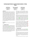
Abstraction using ASM Tools
Olav Jensen, Raymond Koteng, Kjetil Monge, and Andreas Prinz
Faculty of Engineering, Agder University College
Grooseveien 36, N-4876 Grimstad, Norway
[email protected]
Abstract. Abstract State Machines (ASM) are proven to be able to
represent any algorithm at the right level of abstraction. This result
speaks about the running algorithm, i.e. in which way the ASM does the
same steps as the algorithm. However, in practice it is also important to
speak about the description of the algorithm. The purpose of this paper is
to compare the levels of abstraction between ASM and other description
technologies. In order to do this, we formulated a clustering algorithm in
two ASM dialects (CoreASM and AsmL) as well as in ‘mathematics’ and
in Java. We compare the abstraction level of these descriptions and the
strengths and weaknesses of the different languages. The results show
that there is a rather big difference between these languages regarding
syntax, abstraction level, and runtime.
1
Introduction
This paper is a report about an experiment done to check the possibilities of
abstraction in Abstract State Machines (ASM) [1]. In the experiment, we describe a clustering algorithm using ‘mathematics’, two ASM dialects and Java.
We compare the implementations of the algorithms according to the ease of use,
ease of description of abstraction and runtime. Here we will first give a short
introduction to ASM and to clustering.
1.1
Abstract State Machines
Abstract State Machines (ASM) are a formal way to describe algorithms [5].
They are proven to be able to describe any algorithm, and they are even able to
describe them at the right level of abstraction [9].
Abstract State Machines (formerly called evolving algebras) were introduced
by Yuri Gurevich, based on the mathematical concept of algebra and an assignment as the basic way to change between states. ASM have a number of
interesting properties (partly taken from Wikipedia).
Precision Since ASM are based on mathematics, it is clear they provide a
precise way of describing algorithms. Please note that ASM do not come
with a predefined (standard) syntax, but the precision is given in terms
of the underlying semantics. ASMs use classical mathematical structures
to describe states of a computation, and differences between structures to
describe state changes.
2
Faithfulness Given a specification, how does one know that the specification
accurately describes the corresponding real system? Since there is no method
in principle to translate from the concrete world into an abstract specification, one needs to be able to see the correspondence between specification
and reality directly, by inspection. ASMs allow for the use of the terms and
concepts of the problem domain immediately, with a minimum of notational
coding. Many popular specification methods require a fair amount of notational coding which makes this task more difficult.
Understandability How easy is it to read and write specifications using a particular methodology? If the system is difficult to read and write, few people
will use it. ASM programs use an extremely simple syntax, which can be
read even by novices as a form of pseudo-code. Other specification methods,
notably denotational semantics, use complicated syntax whose semantics are
more difficult to read and write.
Executability Another way to determine the correctness of a specification is
to execute the specification directly. A specification methodology which is
executable allows one to test for errors in the specification. Additionally,
testing can help one to verify the correctness of a system by experimenting
with various safety or liveness properties.
Scalability It is often useful to be able to describe a system at several different layers of abstraction. With multiple layers, one can examine particular
features of a system while easily ignoring others. Proving properties about
systems also can be made easier, as the highest abstraction level is often
easily proved correct and each lower abstraction level need only be proven
correct with respect to the previous level.
Generality We seek a methodology which is useful in a wide variety of domains:
sequential, parallel, and distributed systems; abstract-time and real-time
systems; finite-state and infinite-state domains. Many methodologies (e.g.
finite model checking, timed input-output automata, various temporal logics)
have shown their usefulness in particular domains; ASMs have been shown
to be useful in all of these domains.
There exist several tools that implement the ASM methodology. We have chosen
to make our experiments with the CoreASM and the AsmL environments.
CoreASM The CoreASM project [3] is an open source project which is developed by Ph. D. students at the School of Computing Science, Simon Fraser
University, Canada. The goal is to make a formal language which focuses on the
design of an executable abstract state machine, or ASM. CoreASM has support
for high-level design, experimental validation and formal verification of abstract
system models. CoreASM has a plug-in for the Eclipse framework.
AsmL AsmL, or Abstract State Machine Language [7], is a formal language
developed by Microsoft. AsmL is an executable specification language based on
the theory of Abstract State Machines. AsmL is used in situations where precise,
non-ambiguous meaning is important.
3
1.2
Clustering
Data clustering [4] is a common technique for statistical data analysis, which
is used in many fields, including unsupervised machine learning, data mining,
pattern recognition, image analysis and bioinformatics. The main idea with clustering is to classify the objects in question into groups, such that a partitioning
of the data set is reached. Thus clustering is a technique for classification of
objects. A simpler way of saying this is that one should put objects which share
traits or similarities into the same cluster, while objects with different traits
should be put into different clusters. One example of this trait could be Euclidean distance between objects. In our reference book Pattern classification
[4], several algorithms for clustering are given and the properties of all of them
are described. We have picked out a relatively simple algorithm for purposes of
the example. The algorithm we have picked out starts with the idea that initially all objects are associated with arbitrary clusters. The algorithm itself just
picks out an arbitrary element, and tries to place it into another cluster. If this
improves the overall clustering distance, the change is performed. The algorithm
runs until there are no changes over a long period. See chapter 2 for a more
detailed description of the algorithm.
For our purpose it is not necessary to go into details of quality of clustering algorithms, because we just want to compare description properties of the
languages.
1.3
Delimitations and assumptions
There are several possibilities for criteria for clustering, but we will just use for
our example two-dimensional points that are grouped according to geometrical
(Euclidian) distance. One simplifying property of Euclidean distance is that
distances in Euclidean space are symmetric, i.e. the distance from A to B is equal
to the distance from B to A. In order to have a controlled environment to test
and compare the algorithms on different platforms, we have used artificial data
consisting of points in two dimensions, (x,y). By artificial we mean a problem
generated without a specific purpose in mind instead of an existing problem.
1.4
Structure of the Paper
This paper is structured as follows. In section 2, we repeat the definition of
the clustering algorithm given in [4] together with some discussion. Afterwards,
we present an AsmL specification in Section 3 and a CoreASM specification in
Section 4 as well as a Java implementation in Section 5. We present and discuss
our finding in section 6 and present our conclusions in section 7.
2
Description of the Clustering Algorithm
The clustering algorithms we have used in our experiments are described in the
book Pattern classification [4] pages 549 and 550 as follows.
4
The approach most frequently used in seeking optimal partitions is iterative
optimization. The basic idea is to find some reasonable initial partition and to
“move” samples from one group to another if such a move will improve the
value of the criterion function. Like hill-climbing procedures in general, these
approaches guarantee local but not global optimization. Different starting points
can lead to different solutions, and one never knows whether or not the best
solution has been found. Despite these limitations, the fact that the computational
requirements are bearable makes this approach attractive. Let us consider the
use of iterative improvement to minimize the sum-of-squared-error criterion Je
written as:
Je =
c
X
Ji ,
i=1
Where an effective error per cluster is defined to be
X
Ji =
||x − mi ||2
xDi
and the mean of each cluster is, as before,
mi =
1 X
x.
ni
xDi
Suppose that a sample x̂ currently in cluster Di is tentatively moved to Dj . Then
mj changes to
m∗j = mj +
x̂ − mj
nj + 1
and Jj increases to
Jj∗ = Jj +
nj
||x̂ − mj ||2 .
nj + 1
Under the assumption that ni 6= 1(singleton clusters should not be destroyed),
mi changes to
m∗i = mi −
x̂ − m1
ni − 1
and Ji decreases to
∗
J i = Ji −
ni
||x̂ − mi ||2 .
ni − 1
These equations greatly simplify the computation of the change in the criterion function. The transfer of x̂ from Di to Dj is advantageous if the decrease
in Ji is greater than the increase in Jj . This is the case if
5
ni
nj
||x̂ − mi ||2 >
||x̂ − mj ||2 ,
ni − 1
nj + 1
which typical happens whenever x̂ is closer to mj than mi . If reassignment is
profitable, the greatest decrease in sum of squared error is obtained by selecting the cluster for which nj ||x̂ − mj ||2 /(nj + 1) is minimum. This leads to the
following clustering procedure:
Algorithm (Basic Iterative Minimum-Squared-Error Clustering)
begin initialize n, c, m1 , m2 ..., mc
do randomly select a sample x̂
i ←− arg min ||mi − x̂|| (classif y x̂)
if ni 6= 1 then compute
( n
j
||x̂ − mj ||2 if j 6= i
ρj = njn+1
j
2
if j = i
nj −1 ||x̂ − mi ||
if ρk ≤ ρj for all j then transf er x̂ to Dk
recompute Je , mi , mk
until no change in Je , in n attempts
return m1 , m2 ..., mc
end
2.1
Analysis of the Algorithm
When looking at the algorithm, it first turns out that the algorithm does describe
only the clustering itself. When we think of a complete application, we will have
some more work to be done. In fact, a real application is divided into three
different sections; setup phase, algorithm and back-end. The description above
does only talk about the algorithm.
Another comment on the algorithm is that it is not very clear in the description in the text. There it says that one arbitrary point is taken and placed into
another cluster. From the more formal algorithm it can be seen, that in fact the
point is placed into the best cluster available, i.e. the cluster with a centre that
has least distance to this point. The algorithm description does also include a
small problem. The first statement is that the cluster for the chosen point has
to be found. This cannot be done by calculating the distance, but by looking
into the current cluster element sets. We have to take the cluster the point is
included in.1
In our analysis, we will look at the different description methods and how
they are able to cover the complete and correct algorithm for the clustering.
Here we do only want to note that the algorithm description is abstract about
the front-end and back-end parts in that it is not mentioned. This would not be
enough for a complete description.
1
This is a nice argument for executability - if the algorithm written down had been
executable, this error would have been detected.
6
Front-end The front-end phase will be used for initializing the problem by reading a pre-stored problem (set of points) from a file and starting to initialize the
problem. The file contains information about the number of clusters, number of
points and an initial assignment to the clusters. The setup phase is finished with
a visual representation of the problem (see also back-end). Figure 1 shows how
the clusters are initialized before the cluster algorithm starts. We have taken the
same initial clusters for all three approaches. The initial clusters contain random
points, where the points themselves are generated manually. The different colors
indicate the different clusters and a line is drawn from the mean of each cluster
to their points.
Fig. 1. Clustering front-end phase
Algorithm The algorithm part of the framework will do the actual clustering.
The problem is given by the front-end phase and the algorithm starts to work
on the problem. The clustering can be done using CoreASM, AsmL or Java.
Back-end The back-end shall present the results of the algorithm. We use different colors to indicate the clusters and the cluster centre to show how the
cluster looks. This way it is easy to visually evaluate the results of the cluster algorithm. Figure 2 shows the final result of the clustering. All points are gathered
into the four natural clusters that the problem consists of.
3
Implementation in AsmL
AsmL model The AsmL framework is made to work together with the .NET
framework [6]. Therefore AsmL includes several elements that are not directly
related to the original ASM definition. In particular, it is possible to define
7
Fig. 2. Clustering back-end phase
classes and methods using AsmL. However, most of the basic ASM functionality
is still available. Because we want to stay as close to ASM as possible, in our
AsmL description we do not use classes. This also makes it easier to compare the
AsmL and CoreASM solutions. The first thing to define in ASM and thus also
in AsmL is related to the structure of the problem. As we want to describe state
transitions, we have to describe the state first. This means in our case that we
have to define cluster and point which are structures. The point structure has two
Integer elements x and y containing the x and y location values of the point. The
cluster structure has three elements: one set of included points, one center point
named centerPoint and a variable for storing the clusters sum-of-squared-error
value (SSR).
The use of structures proved very helpful for the description, because these
are the units of understanding of the algorithm. In standard ASM, a structure
relates to an abstract object having an access function for each of the structure
fields. But then again, having a structure in a set does not allow to change its
fields. This was at times unhandy for our problem.
Syntax The AsmL syntax structure is built on indentation. A sequential ASM
step is declared by the keyword ‘step’ followed by the (parallel) code for the
step. Updates to variables will be performed after the step has been processed.
Internally it seems that code is read sequentially, while the updates within a
single step are performed simultaneously. So that in the step below,
step
WriteLine(’’foo’’)
WriteLine(’’bar’’)
X := Y
Y := X
8
foo will always be printed in the console before bar. But the updates to the
variables x and y are performed at the same time, effectively setting x to the old
value of y and y to the old value of x. This is consistent with the ASM model.
One should not need to worry about how the steps are performed in details, only
that the more abstract ideas does what it’s supposed to do. Indentation can be
a confusing way of defining blocks of code. One seemingly small error might be
hard to spot, but could change the way the entire specification performs.
The description for calculating the SSR (Ji ) in AsmL is as follows.
calculateSSR(c as Cluster) as Double
var ssr as Double = 0.0
step foreach p in c.pts
ssr := ssr +(((p.x - c.centerPoint.x)*(p.x - c.centerPoint.x))+
((p.y - c.centerPoint.y)*(p.y -c.centerPoint.y)))
step return ssr
It should be noted that AsmL introduced a special notation for sequentially
running through a collection of objects, which is the ‘foreach’ construct used
above. This will lead to a sequence of steps.
The description of the impact of adding or loosing one point to a cluster (ρj )
is as follows.
let tmp = if (exists p1 in c.pts where p = p1) then -1 else 1
return Size(c.pts)/(Size(c.pts)+tmp)*dist(p,c)
Finally, the main algorithm looks like this.
clusterStep()
choose c1Tmp as Cluster in clusters where Size(c1Tmp.pts) > 1
choose p in c1Tmp.pts
choose c2Tmp in clusters where
forall cc in clusters
holds newSSR(c2Tmp,p) <= newSSR(cc,p)
var c1 = c1Tmp
var c2 = c2Tmp
step
if (c1<>c2)
let increase = increaseSSR(c2,p)
let decrease = decreaseSSR(c1,p)
let hlpssr1 = calculateSSR(c1)
let hlpssr2 = calculateSSR(c2)
if (decrease > increase)
step
c2.ssr := c2.ssr+increase
c1.ssr := c1.ssr-decrease
add p to c2.pts
remove p from c1.pts
c2.centerPoint := updateMeanAdd(c2,p)
9
c1.centerPoint := updateMeanSub(c1,p)
totalSSR := (totalSSR + increase - decrease)
remove c1Tmp from clusters
remove c2Tmp from clusters
step
add c1 to clusters
add c2 to clusters
step
iTotalRuns := 1 + iTotalRuns
if (iRuns = iterationCount)
if (oldSSR > totalSSR)
oldSSR := totalSSR as Double
iRuns := 0
else
bFinished := true
else
iRuns := iRuns + 1
Front-end and Back-end In order to handle front-end and back-end, we could
use AsmLs embedding in .NET. This means it is possible to create a library
using C#.NET for reading files and displaying the results. In order to have
a most unique display of the results, we have chosen to stream all result via
the Java interface, such that for AsmL we had to write out the result for later
use in Java. Because AsmL is a Microsoft based program we were not able to
link this directly to the framework that we have made in Java. However the
SpecExplorer program creates an .EXE file from the compiled project which can
be started directly from the framework. To be able to present the results in the
same framework we have created an XML generator from the .NET library. This
XML generator is included in the AsmL project and creates an XML file from the
clustering results, which we can open manually from our main framework. This
way we can give a visual representing from the experiments in our framework
when the actual clustering is done.
4
Implementation in CoreASM
CoreASM model CoreASM is supposed to be a very faithful implementation
of the original ASM ideas [2]. This means, for example, that instead of objects
and methods, in CoreASM one has to define functions and rules. For instance:
The SSR value of a cluster is defined as a function which takes a cluster as input
and gives a value as output.
Syntax The CoreASM syntax structure is build on blocks of parallel code defined by the keywords par and endpar. Updates will be performed after the entire
par -block has been processed. To achieve sequential specifications one has to use
10
the turboASM plug-in, which enables the keywords seq and next. Combining
seq/next and par/endpar it is possible to create advanced steps which themselves contains internal sub-steps. Defining blocks of code within two keywords
gives nice and clean code, but the seq/next can be confusing at times and some
complex specifications might contain a lot of seemingly unnecessary seq/next
keywords, often nested inside other steps. To us it seems that these keywords
could be dropped entirely. Since it is not allowed to have two par/endpar blocks
after one another anyway (it makes no sense to do so unless they should be
performed sequentially) one could just assume that two par-blocks should be
handled as two sequential steps in an ASM model.
The specification of calculating the SSR in CoreASM is as follows.
rule funSSR(cluster) = return
SUM({x is (dist(p,cluster)) | p in points(cluster)}) in skip
This specification uses a function SUM, which adds all the elements in a list.
This kind of function is not yet part of the CoreASM standard distribution, but
could be specified as follows.
rule SUM(s) =
return res in
seq res:=0
seq hlp:=s
while (not (hlp={}))
choose e in hlp do
par
remove e from hlp
res:=res+e
endpar
Of course, this is a messy description of something simple. It would be better to
have some kind of iterator concept in CoreASM to describe this. A new mathplugin has been created by the CoreASM developers which solved the SUM, but
it does not provide a general iterator solution.
The formula for the impact of adding or loosing one point to a cluster is in
CoreASM:
return dist(p,c)*|points(c)| /
(|points(c)|+((p memberof points(c))?(-1):1)) in skip
And finally the algorithm is in CoreASM as follows.
rule clusterStep =
seq choose c in clusters with (|points(c)| > 1) do
choose p in points(c) do //select a random point from c
choose c2 in clusters with
forall cc in clusters
holds newSSR(c2,p) <= newSSR(cc,p)
11
do
if not (c=c2) then
let increase = newSSR(c2,p), decrease = newSSR(c,p) in
if ( decrease > increase ) then
par
add p to points(c2)
remove p from points(c)
ssr(c2) := ssr(c2)+increase
ssr(c) := ssr(c)-decrease
totalSSR := totalSSR + increase - decrease
updateMean(p,c,c2)
endpar
Front-end and Back-end Because CoreASM still is at a beta level there is no
plug-in that supports linking from CoreASM directly to Java or to write to a file.
This means that we cannot start or get any information from CoreASM directly
to our framework. To solve this problem we have implemented a method in
our main framework that can generate the initial problem to CoreASM source
code. This code can be copied into our fornt-end phase (one special rule) of
the program. When the algorithm has finished clustering, CoreASM writes the
results from the clustering to the console. This output can be copied into our
CoreASM-to-Java parser. The back-end part will read this file and parse the
information needed to Java objects. These objects can be displayed in our main
framework so it is easy to evaluate the results.
5
Implementation in Java
Java is a common programming language and the framework has a large set of
libraries for developing application. Therefore Java also has another structure
than ASM languages. This application is created in a more traditional software
development style. The framework and the algorithm are developed in an objectoriented way with all classes stored in different packages. The clusters are stored
in vectors and have a list that has a reference to the points that the cluster
consist of. Each time a point is moved this list will be updated. Each cluster is
stored in a class “Clusters” which also holds the value of the center point and
the clusters SSR value.
Syntax The Java syntax is a high level programming language. It is fully objectoriented and all source code is written inside a class.
Writing the algorithm in Java was different from the ASM versions in that
the Java code really does move the point and then checks if that made a positive
difference and possibly undoes the change.
The specification of SSR calculating in Java is like this.
12
SSR = 0;
for(ClusterPoint point : this)
{
double pointDistance = point.getDistanceToPoint(middle);
SSR += pointDistance;
}
The formula for the impact of adding or loosing one point to a cluster is using
the old and the new size which is available because the point is really moved.
double newSSR = oldSSR+iOperator+
sizeOld / sizeNew * pointDistance;
And finally here is the code for the main algorithm in Java.
while(true) // find first cluster
{ iFirstCluster = clusters.getRandomCluster();
if(clusters.elementAt(iFirstCluster).size() > 1) break;
}
while(true) // find second cluster
{ iSecondCluster = clusters.getRandomCluster();
if(iFirstCluster != iSecondCluster) break;
}
Cluster cluster1 = clusters.elementAt(iFirstCluster);
Cluster cluster2 = clusters.elementAt(iSecondCluster);
int idPoint1 = cluster1.getRandomPointId();
ClusterPoint point1 = cluster1.elementAt(idPoint1);
distBeforeMove =
cluster1.getTotDistance() + cluster2.getTotDistance();
double[] newMiddleCluster1 = cluster1.getMiddle().clone();
double[] newMiddleCluster2 = cluster2.getMiddle().clone();
double oldDistanceCluster1 = cluster1.getTotDistance();
double oldDistanceCluster2 = cluster2.getTotDistance();
int iCluster1Size = cluster1.size();
int iCluster2Size = cluster2.size();
iCluster1Size--; iCluster2Size++;
double point1MiddleCluster1 =
point1.getDistanceToPoint(newMiddleCluster1);
double point1MiddleCluster2 =
point1.getDistanceToPoint(newMiddleCluster2);
cluster1.updateDistances
(false,point1MiddleCluster1,iCluster1Size);
cluster2.updateDistances
(true,point1MiddleCluster2,iCluster2Size);
newMiddleCluster1 = cluster1.updateMidle(false,point1.getValues(),
newMiddleCluster1,iCluster1Size);
newMiddleCluster2 = cluster2.updateMidle(true,point1.getValues(),
13
newMiddleCluster2,iCluster2Size);
distAfterMove =
cluster1.getTotDistance() + cluster2.getTotDistance();
if(super.checkSwitch()) // is this a good move?
{ cluster2.add(point1);
cluster1.removeElementAt(idPoint1);
cluster1.setValues(newMiddleCluster1.clone(),
cluster1.getTotDistance());
cluster2.setValues(newMiddleCluster2.clone(),
cluster2.getTotDistance());
} else { // Bad move
cluster1.setValues(cluster1.getMiddle(), oldDistanceCluster1);
cluster2.setValues(cluster2.getMiddle(), oldDistanceCluster2);
}
Front-end and Back-end Our framework is written in Java and therefore we
did not have any problems implementing the algorithm into this framework. The
algorithm is stored in a separate package and can be started and stopped easily
from the framework. It is not a problem to get access to all data to give a visual
representation for our clustering.
6
Discussion
In this chapter we will discuss the abstraction levels of the formal languages. We
present results from our experiments done to measure speed and compiler time
and finally we describe our solution for the different parts of the framework.
As a general remark it has to be said that this is a work of computer science
master students. There were the usual problems with ASM, in particular that it
was difficult to understand that in ASM all updates, if not otherwise described,
are done in parallel. This was solved after some frustration over inconsistent
update errors. In fact, it turns out that a lot of thinking is needed to get the
parallel and sequential parts correct. Often the solution is overly sequential just
because the correct parallelism is too difficult to get correct.
The work was done in first writing a Java program, then the AsmL specification, then the CoreASM specification. Therefore it can be expected that
the latter descriptions have higher abstraction levels as they went through more
iterations.
6.1
Abstraction level
The most verbose of the specifications was the Java specification, containing lots
of details the other specifications did not describe. The next level were the ASM
specifications and finally the original text description is the highest level.
The levels of abstractions of the CoreASM and AsmL languages are slightly
different. Because of the object-oriented features made available in AsmL it
14
can be said that AsmL is more a sort of crossbreed between a programming
language and the ASM theory than CoreASM is. This makes AsmL better suited
for software testing with regards to the actual code level while CoreASM with
a higher abstraction level is better suited to specification with regard to the
problem. CoreASM is most likely better suited for use early in the software
engineering stages while AsmL is better suited at a later stage [8].
Fig. 3. Level of abstractions
We have counted the number of source code lines that we needed in order
to describe the algorithm in these languages. The result is shown in the table
below. The table shows the number of source code lines needed in the respective
languages. As expected, a full implementation needs more source code than ideas.
Language
Idea
CoreASM
AsmL
Java
front-end
230
55
545
algorithm
11
82
155
360
back-end
1244
275
1067
Fig. 4. Code size of different abstraction levels
Please remember that the contents of the front-end and back-end is different for
the different languages, so this is not really a fair measure.
6.2
Speed
Because the formal languages, especially CoreASM, have a really slow compile
we have chosen to measure this. The results from the compiler measures are
15
showed in the table below. Finally, we have measured the runtime each language
spends on the different problems. The results in the table below show that it is
a rather big difference between the languages.
Language
CoreASM
AsmL
Java
compile time
8.25 seconds
5 seconds
3.1 seconds
runtime 50 points
54.4 seconds
4.9 seconds
41 milliseconds
runtime 100 points
157.5 seconds
16 seconds
56.7 milliseconds
Fig. 5. Time comparison between different abstraction levels
6.3
Support
AsmL The AsmL language can be used as a functional programming language.
Its object-oriented functionality made it quite easy for us (being object-oriented
programmers) to get an understanding of it. It is reasonably well documented,
but the online community seemed somewhat small. So we had to use some of the
try and fail method to get a decent understanding. Even after being able to write
and test the algorithm there are still some issues that baffle us. The code we have
written works well when running SpecExplorer in debug mode, even if it never
reaches any break points. But when running the code without debugging, it does
not, objects and variables do not seem to be initialized outside the step they were
declared in. Why this happens we have never discovered. We also noted the lack
of any syntax highlighting or similar tools in SpecExplorer. This combined with
the importance of indentation in AsmL made it confusing at times, but this was
more of an annoyance than a real problem. On the other hand SpecExplorer does
have support for debugging, which is a very nice feature to have when trying to
understand how a language works by seeing how the specification behaves step
by step. In ASM the action of going from one state to another is called a step.
All updates done in a step are done in parallel. In AsmL a step is defined by
the keyword step and the rest of the block with one or more whitespaces. We
had some trouble with these spaces, a few times code lines were written with the
wrong amount of spaces. This could result in compilation errors, or just wrong
results, the latter being hard to discover.
CoreASM To write, compile and run CoreASM specifications we used an
Eclipse plug-in. After working in SpecExplorer it was a relief to find that we now
had syntax highlighting. This makes the code much easier to read and maintain.
There was a downloadable version of the CoreASM user manual, which helped
us a lot, but it mostly explains the syntax of the different rules and plug-ins
available and not much information on the language in a way that is suitable for
beginners. In fact, detailed ASM explanations suitable for beginners are hard to
find. There are also some example specifications available from the CoreASM
16
project page which helped us to get started. However, once we needed to do
things not directly explained in the manual or in the examples we had to resort
to the try and fail method. This is a very slow and tiresome way of learning. CoreASM is built with a kernel containing the minimum of vocabulary and rules to
create a CoreASM specification. All other rules have to be imported as plug-ins.
Most of these plug-ins can be imported with the use of StandardPlugins instead
of having to import all the plug-ins specifically. There are a few non-finished
plug-ins that, if used, need to be specifically imported. All of these plug-ins are
explained in the user manual. In CoreASM a block of parallel code is written
between par and endpar keywords. Everything in a par-block is updated as one
step. When there is need for sequential updating a plug-in called TurboASM
Plug-in has to be used. TurboASM allows for one rule to be updated before the
next rule. In other words, a rule is executed then a step is made and the next
rule is executed. The syntax for this is seq rule1 next rule2. The next keyword is
optional and is available to make the code easier to read. One of the problems we
encountered with this syntax was where there had to be more than two sequential updates. In those cases we used a sequence block inside a sequence block.
Utilizing this it is possible to have as many sequential updates as one desires,
but the code will not be very readable with more than two or three sequential
blocks.
One big problem with CoreASM was the speed. For some reasons CoreASM
spends a lot more time on problems than Java. From the speed part we can see
that Java uses around 40 milliseconds on the same problem that CoreASM uses
almost one minutes to solve. We have not found out why it is so much difference
in the time spend on the problem. However, we used CoreASM to formally prove
that the algorithm is working as expected and therefore we do not consider time
to be an important issue in this experiment.
7
Conclusion
Formal languages can be very helpful when it comes to testing and proving both
abstract ideas and less abstract algorithms without having to fully implement
them. However, in order to get algorithms correct it is essential to have the
possibility to try them out. This is what we call executability. In practice, executability includes more than just the availability of an interpreter. One has to
take care of the user and needs to provide a proper front-end and a back-end.
ASM does not care for these parts, as they have nothing to do with the
algorithm specification. This leads to the difficult situation that a user has to take
care of them on her own. In our experiments we have seen that it is important to
provide good and strong support for external libraries - either as an integration
with another language as in the case of AsmL or by providing proper functions
and libraries in the language itself.
When it comes to the specification properties, the text specification was
clearly the most abstract, but it also omitted important details. The AsmL and
CoreASM specifications were almost on the same level, although AsmL allows
17
the expression of more low-level details than CoreASM. Java is clearly the most
detailed of these candidates.
However, it turns out that some of the abstractness of ASM is lost because
ASM do not provide support for modern patterns of software engineering as
iterators and interfaces, maybe even object-orientation. It was also clear that
the distinction between parallel and sequential steps is not always trivial and
guidelines for this are largely missing.
Our experiment has also shown that syntax is very important, and that the
semantic proof of ASM being able to represent all algorithms still has some
challenges when one wants to put it into real syntax.
References
1. Egon Börger and Robert Stärk. Abstract State Machines. A Method for High-Level
Design and Analysis. Springer, 2003. ISBN: 3-540-00702-4.
2. Roozbeh Farahbod. CoreASM - an extensible ASM execution engine. Web page.
See http://www.coreasm.org/index.php.
3. Roozbeh Farahbod. CoreASM user manual. PDF document. See
https://sourceforge.net/projects/coreasm.
4. Gouri K. Bhattacharyya, Richard A. Johnson. Pattern classification 2. Edition.
John Wiley & Sons, Inc, 2001. ISBN: 0-471-03532-7.
5. Jim Huggins. Abstract state machines. Web page. See
http://www.eecs.umich.edu/gasm/.
6. Microsoft. Asml. Web page. See http://research.microsoft.com/fse/asml/.
7. Microsoft. AsmL manual. Web page. See
http://research.microsoft.com/foundations/asml/.
8. Roozbeh Farahbod, Vincenzo Gervasi, and Uwe Glässer. Design and Specification
of the CoreASM Execution Engine. PDF document. See also
http://www.cs.sfu.ca/ se/publications/CMPT2005-02.pdf.
9. Yuri Gurevich. Sequential Abstract State Machines capture sequential algorithms.
In ACM Transactions on Computational Logic,1(1):77-111, 2000. ISSN: 1529-3785.