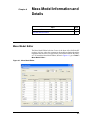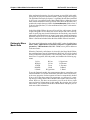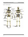
1
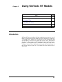
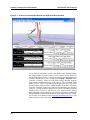
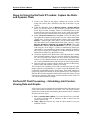
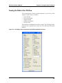
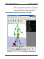
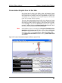
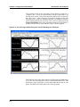
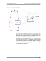
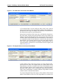
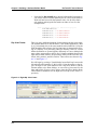
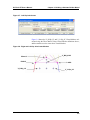
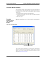
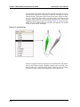
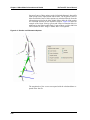
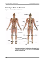
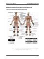
User’s Manual
Motion Analysis Corporation: Software License Agreement Terms and Conditions
Definitions
The following terms are defined for the purpose of this Agreement as follows:
(a) “Designated System” means the specified computer system described on the facing of this agreement, which Licensee has
purchased from the Licensor.
(b) “Licensed Program” means the software program described on the facing page of this Agreement in object code form only,
any updates subsequently provided by License, all permitted copies made by Licensee, and all basic or related materials
pertinent to such programs.
License
Under a license granted under this Agreement, License is authorized, on a non-exclusive basis, to use the Licensed Program on
the Designated System. License shall refrain from taking any action, such as reverse assembly or reverse compilation, to derive
a source code equivalent of the Licensed Program. A license shall be valid until terminated under this Agreement. The license
fee is part of the purchase price of the Designated System.
Title
The original, and any copies of the Licensed Program, in whole or in part, which are made by Licensee, are the property of
Licensor.
Copies
With each license, Licensee may make one (1) copy of the Licensed Program in object code form only for use by Licensee with
the Designated System for backup or archive purposes. Licensee agrees to maintain records of each copy of the Licensed
Program and the serial number of each computer system with which the Licensed Program is incorporated or used.
Copyright Protection
The Licensed Program is copyrighted by Licensor. Copies may be made only as permitted by this Agreement. Licensee agrees
to reproduce and apply the copyright notice and proprietary notice of Licensor to all copies, in whole or in part, in any form, of
Licensed Program made hereunder.
Warranty Exclusion
Any maintenance obligations of Licensor shall be subject to a separate maintenance or update agreement between and
licensee.
LICENSOR MAKES NO WARRANTIES, EITHER EXPRESS OR IMPLIED ON ANY LICENSED PROGRAMS, AND
EXPRESSLY DISCLAIMS ALL IMPLIED WARRANTIES OF MERCHANTABILITY AND FITNESS FOR A PARTICULAR
PURPOSE.
Patent and Copyright Indemnification
Licensor shall indemnify Licensee against liability for patent and copyright infringement upon the terms and conditions
applicable to Licensee’s purchase of the Designated System.
Termination
This agreement and any licenses granted hereunder may be terminated by Licensor upon written notice if Licensee fails to
comply with any of the terms and conditions of this agreement. Upon termination of any license, Licensee will, at Licensor’s
option, either return the Licensed Program to Licensor, or destroy the original and all copies and parts thereof.
General
This agreement is not assignable. The rights under this Agreement or any license granted hereunder may not be assigned,
sublicensed or otherwise transferred without the prior written consent of Licensor. Except as otherwise specified herein, this is
the entire agreement between the parties relating to the subject matter hereof and may only be modified in writing signed by
each party. This agreement is governed by the laws of the State of California.
For further information regarding this KinTools RT User’s Manual or other products, please contact:
Motion Analysis Corporation
3617 Westwind Boulevard
Santa Rosa, CA 95403 USA
tel: 707.579.6500
fax: 707.526.0629
[email protected]
P/N 666-1020-020
www.motionanalysis.com
Copyright © 2010
Table of Contents
Chapter 1
Introduction
Overview .......................................................................................... 1-1
For More Information ........................................................................ 1-2
Chapter 2
Using KinTools RT Models
Introduction....................................................................................... 2-1
Steps for Using the KinTools RT models: Capture the Static and
Dynamic Trials ............................................................................ 2-3
KinTools RT Post Processing – Calculating Joint Centers, Viewing
Data and Graphs ........................................................................ 2-3
Seeing the Data in the 3D View........................................................ 2-5
Presentation Graphs View of the Data ............................................. 2-7
Chapter 3
Building a Skeleton Builder Model
KinTools RT Modeling....................................................................... 3-1
Defining Skeleton Builder Segments .............................................. 3-10
Chapter 4
Mass Model Information and Details
Mass Model Editor............................................................................ 4-1
Calculate Kinetics Button ................................................................. 4-7
Appendix A
Marker Set Placement
Helen Hayes Marker Set Placement ................................................ A-2
Modified Cleveland Clinic Marker Set Placement ............................ A-3
Appendix B
Overview of Calculations
Introduction....................................................................................... B-1
Source of Forces and Moments on Segments ................................. B-2
Three-Dimensional Inverse Dynamics Analysis ............................... B-2
Solving for the Unknowns................................................................. B-3
Appendix C
Sample Pictures
Appendix D
Works Cited
1
KinTools RT User’s Manual
2
Chapter 1
Introduction
Topic
Page
Overview
1-1
For More Information
1-2
Overview
KinTools RT is a full-body, three-dimensional engine capable of calculating kinematic and kinetic information on models that are created and
saved in the project file(s). The kinetic calculations can be done on either
of the two skeleton types available in Cortex: Skeleton Builder and Calcium. The Skeleton Builder models are generally simpler to use as they
automatically scale the bone lengths to the subject’s actual bones, so these
are the models that are included and discussed. The Calcium based models use an entirely different computation method of Global Optimization.
The results are similar if care is taken using either skeleton model.
The Cortex KinTools RT release includes two human models with more
and less detail. These models are built using the Skeleton Builder (abbreviated SkB) modeling software in Cortex. Skeleton Builder enhancements
for Cortex include two important new features to aid in building models:
1. User defined Euler angle rotation order
2. User definable Bone Axis
Cortex has three check boxes above the Post Processing “Calculate” button:
1. The Calculate VMs check-box is selected to calculate the Virtual
Marker locations using Cortex.
2. The Skeleton check-box tells the software that you would like to Cal-
culate the joint angles or kinematics of the skeleton defined in your
project using Skeleton Builder.
3. The Kinetics check-box tells the software to use the subject’s weight
along with the entries in the Mass Model Editor table to calculate the
forces and moments for each segment or bone in the model. The
forces and moments are first calculated from the center of mass of
each segment in the global coordinate system, and then translated to
the joint center at the end of the bone. This information is accessed
through KinTools RT.
1-1
Chapter 1: Introduction
KinTools RT User’s Manual
For More Information
Please contact Motion Analysis Customer Support with any questions,
problems, or feedback about the Motion Analysis KinTools RT software.
We can be reached at:
Motion Analysis Corporation
3617 Westwind Blvd.
Santa Rosa, CA, USA 95403
Phone: 707-579-6500
Fax: 707-526-0629
http://www.motionanalysis.com
For technical support and licensing information, please contact:
[email protected]
For information about sales, please contact:
[email protected]
1-2
Chapter 2
Using KinTools RT Models
Topic
Page
Introduction
2-1
Steps for Using the KinTools RT models: Capture the Static
and Dynamic Trials
2-3
KinTools RT Post Processing – Calculating Joint Centers,
Viewing Data and Graphs
2-3
Seeing the Data in the 3D View
2-5
Presentation Graphs View of the Data
2-7
Introduction
KinTools RT has two built-in full body models that you can use “out of
the box” based on two popular marker sets: the “Helen Hayes” and/or the
“Cleveland Clinic” marker sets. The models are fully configurable and
also included is a full suite of graphs that use the Cortex Presentation
Graphs tools. The complete model, including the Mass Model for kinetics
properties, is stored in the Cortex 2 “MarkerSet” and is part of the Cortex
2 software release. These MarkerSets can be seen and selected for use in
the System Objects panel as: ClevelandClinic.mars and/or HelenHayes.mars.
2-1
Chapter 2: Using KinTools RT Models
KinTools RT User’s Manual
Figure 2-1. 3D View and Presentation Graphs with Right Foot Bone Selected
To use either or both models, start by viewing the sample data provided in
the Samples folder, also part of the Cortex 2 software release. When you
run the Setup file for Cortex 2, you also the Samples and Tutorial data sets
installed, including this User’s Guide from the Help > Tutorials menu.
Load the “Captures” shown in each folder and get familiar with the
marker names and the placement of the markers. The Cleveland Clinic
marker set uses “cluster” type markers on the upper and lower legs while
the Helen Hayes marker set uses markers attached to the skin. Sometimes
viewed as “minimal” marker sets, each one has advantages. See the steps
below for viewing the data in different ways in the 3D and Presentation
Graphs panels of Cortex 2. All users can view and process the sample
data using these built-in models but you must have licenses for editing the
SkeletonBuilder or Mass Models that are used in KinTools RT. Temporary licenses are available; contact [email protected] or your
Motion Analysis salesperson with your request.
2-2
KinTools RT User’s Manual
Chapter 2: Using KinTools RT Models
Steps for Using the KinTools RT models: Capture the Static
and Dynamic Trials
1. Create a new folder for the capture, calibrate the system, save the
Setup with a name (like Calibrated or the date or the name of your
subject).
2. Select the MarkerSet from the Motion Capture > System Objects
panel. Use the blue arrow to copy from the System Objects to the
Local Objects folder. Example: Select ClevelandClinic.mars in the
System Objects panel; use the blue arrow to copy to the Local folder.
Note it becomes the selected marker set in the Local Objects panel.
3. Select Connect to Cameras and then Run. Collect the Static Trial
and update the template for this person. Have the subject stand in the
“Model Pose” position. From the Motion Capture panel, select New
Subject… (bottom right) which shows you the current Model Pose.
Have the subject move around until the stick figure “snaps in”. Check
Refit the Identifying Template and Update the Model. Then click
Pause, Run, and then Save the MarkerSet. If you are not familiar
with using the “New Subject..” feature to automatically identify the
static markers, you can collect a Static1 Capture, Identify the markers
and Create or Update the Template in Post Processing then Save the
MarkerSet from the File or QuickFiles menu.
4. Collect the Dynamic trials. Both of these full body models use medial
knee and ankle markers which are removed during the Dynamic trials. The Cleveland Clinic marker set also removes the lateral knee
markers. Use the updated template to automatically identify the markers or collect unnamed markers and edit later for trials with good data.
5. After the trials are captured, edit the marker data in Post Processing.
Edit the Static and Dynamic Captures, save them.
This completes the capturing session and is no different from any other
capture sequence except that there is a “Static” trial with additional markers that help in calculating accurate joint centers. These static markers are
removed to simplify the marker set for the dynamic trials. The strength of
KinTools RT becomes apparent in the Post Processing side where you can
calculate the kinematic and kinetic variables and show them in the 3D
view and on the Presentation Graphs.
KinTools RT Post Processing – Calculating Joint Centers,
Viewing Data and Graphs
A Sky script is used to automate the calculation of the joint centers based
on the static marker placements in the Static Trial. The offsets from the
markers that remain on the person during the dynamic trial are calculated
from the static trial. Steps:
1. File > Load the Static capture. View and edit and save as needed.
No need to Calculate VMs or Skeletons as this is done in the Sky
script in the next step.
2. Tools > Sky and select the sky script for either marker set (or your
modified version).
2-3
Chapter 2: Using KinTools RT Models
KinTools RT User’s Manual
From the Global Sky Scripts > KinTools RT folder, select either
CC_StaticToDynamic.sky for the Cleveland Clinic MarkerSet, or
HH_StaticToDynamic.sky for the Helen Hayes MarkerSet.
3. Click the Run button (Center of the Sky scripting interface’s top line).
Note:
If you make a mistake or are not sure, load the static capture again and
then run the Sky script again.
The script calculates the Virtual Marker locations, and remembers the locations of the static markers with respect to the remaining dynamic markers. It then updates and saves the MarkerSet file in the current folder. You
can see the steps as they happen in the middle bottom “Output” panel of
the Sky scripting interface. The “Clear Output” is the top right command
to the right of the Run button.
4. Process each dynamic trial:
File > Load Capture. Check VMs, Skeleton, Kinetics, and click Calculate.
Figure 2-2. Calculate Button with All Three Check Boxes Active
2-4
KinTools RT User’s Manual
Chapter 2: Using KinTools RT Models
Seeing the Data in the 3D View
3D Viewing Options—For the selected segment(s), you can view at the
segment’s center of mass 5 variables:
•
•
•
•
•
Linear Velocity
Linear Acceleration
Angular Velocity
Angular Acceleration
Gravity Vector
The Joint Forces and Moments can also be shown. The 3D Display Show
properties box is shown below with ALL of the KinTools RT options
checked.
Figure 2-3. 3D Display—Show Properties with All KinToolsRT Boxes Active
2-5
Chapter 2: Using KinTools RT Models
KinTools RT User’s Manual
Which gives a complete model with all options and all segments shown in
Figure 2-4. Angular velocities and accelerations are shown as disks with
two colors for showing positive and negative data. Linear Velocities and
Accelerations and Gravity are shown as vectors at the segment’s center of
mass. Joint Forces and Moments are shown as vectors and disks.
Figure 2-4. 3D KinTools Display with All Segments and Display Options ON
2-6
KinTools RT User’s Manual
Chapter 2: Using KinTools RT Models
Presentation Graphs View of the Data
New in the Cortex 2 release is the ability to show the kinematic, kinetic
(and other) data in user-definable “Presentation Graphs”. The KinTools
RT example data set includes a full suite of graphs that are yours to use
and modify. To see the graphs, Load a Capture and press the Calculate
(with VMs, Skeleton, Kinetics checked).
To see the data in the graphical form for all cycles, choose two layouts
with 3D on top and Presentation Graphs on the bottom. Right click in the
Presentation Graphs window to bring up the options for the graphs.
Choose Settings… and select the Open Icon (top left) on the “Graph Appearance” window. Navigate to \Cortex2\Samples\KinTools RT Cleveland Clinic MarkerSet\SkeletonBuilder_Gait.graphs.
Note:
On WinXP, this Cortex2 is located in the C:\Program Files\Motion Analysis folder. On Windows 7 and Windows Vista, look in C:\ProgramData\Motion Analysis\Cortex2.You will first need to make the ProgramData folder visible. See the Control Panel > Search for Hidden Files …
select Hidden Files and Folders and then select: ( ) Show Hidden Files
and Folders.
Figure 2-5. Bottom Presentation Graphs for Entire Capture Time
2-7
Chapter 2: Using KinTools RT Models
KinTools RT User’s Manual
To get a better look, at any one graph, use the hotkey 9 toggle for a
“Graphics Only” screen (no control buttons) and press Space bar to get
the full screen on the selected Presentation Graphs panel. To show the
data “By Cycles”, right click in the Presentation Graphs window and
check the Draw Cycles box. With these options, you should see a Presentation Graphs panel like the one below. The Cycles are defined from the
Tools > Event Editor which along with the Presentation Graphs feature is
available for all Cortex 2 users with their Cortex 2 license upgrade.
Figure 2-6. Hip Joint Angle with Draw Cycles Checked Showing One Gait Cycle.
Other options in the right-click menu for the Presentation Graphs allow
you to save the selected graph’s data in a tab-delimited ASCII file, Add
and Remove pages (each page is a tab) and sending the bit map to your
printer with the best looking results from a full page graph.
2-8
Chapter 3
Building a Skeleton Builder
Model
Topic
Page
KinTools RT Modeling
3-1
Defining Skeleton Builder Segments
3-10
KinTools RT Modeling
Building a KinTools RT model in Cortex involves three separate and sequential steps:
1. Defining Joint Centers (using Virtual Markers)
2. Defining Skeleton Builder Segments
3. Specifying the Mass Model to be Used (discussed in Chapter 4, Mass
Model Information and Details)
Defining Joint
Centers
Joint centers in KinTools RT are defined using Virtual Markers, of which
there are five types:
1.
2.
3.
4.
5.
Three Marker Value
Three Marker Ratio
Two Marker Value
Two Marker Ratio
One Marker Value
The majority of Virtual Markers used to define joint centers will use the
Three Marker Value and Two Marker Ratio definitions, although other
Virtual Marker definitions may be used. Figure 3-1 shows the Virtual
Marker Definitions Edit box.
3-1
Chapter 3: Building a Skeleton Builder Model
KinTools RT User’s Manual
Figure 3-1. Virtual Marker Definitions Edit Box
Although there are many ways to define a joint center, joint centers in
KinTools RT will be defined by locating the boundaries of a joint (i.e.,
medial and lateral landmarks), and creating a landmark half the distance
between those two markers. In general, joint centers can be defined by the
following formula:
,
where C is the location of the joint center, Lm is the lateral joint marker,
Mm is the medial joint marker, and p is the percentage offset between the
lateral and medial joint markers [2]. It is worth noting that the hip joint
center is defined differently, and will be discussed later. A simple example of this definition is the knee joint. The knee joint is defined by placing
markers on the lateral and medial femoral condyles and then creating a
joint center half way between these markers. See Figure 3-2 on the next
page for an example.
3-2
KinTools RT User’s Manual
Chapter 3: Building a Skeleton Builder Model
Figure 3-2. Knee Joint Center Marker
The Lateral Knee and Medial Knee markers are used to define the Knee
Joint Center marker. A Two Marker Ratio Virtual Marker with the Lateral
Knee marker set to the Origin Marker and the Medial Knee marker set to
the Long Axis Marker. The Knee Joint Center is located 50% of the distance between the Lateral Knee and Medial Knee markers.
To create the joint center illustrated in Figure 3-2, a Two Marker Ratio
Virtual Marker is used. This type of Virtual Marker definition is defined
by locating the Origin and Long Axis Markers, and then specifying the
percent offset along the long axis from the Origin Marker (see the formula
on the previous page). Figure 3-3 on page 3-4 uses the joint center definition from above to show how the Left Knee Joint Center is created using a
Two Marker Ratio Virtual Marker.
3-3
Chapter 3: Building a Skeleton Builder Model
KinTools RT User’s Manual
Figure 3-3. The Static Knee Joint Center Virtual Marker.
A Two Marker Ratio is used to define the Knee Joint Center, with the
L.Knee (lateral marker) as the Origin Marker and the L.Knee.Medial (medial marker) as the Long Axis Marker. The joint center is located 50% of
the distance between the two specified markers.
Notice that the Left Knee Joint Center above is defined by using the medial joint marker. During many Biomechanical studies, the medial joint
marker is removed after the static trial for various reasons. This causes the
Left Knee Joint Center definition to become undefined. For this reason, it
is essential that another Virtual Marker be created in the same location
that will allow us to track the location of the joint center during dynamic
trials. This second Virtual Marker, or Dynamic Virtual Marker, will use
segmental markers assumed to be a fixed distance from the original joint
center. See Figure 3-4.
Figure 3-4. The Dynamic Knee Joint Center Virtual Marker
A Three Marker Value (with snap-to feature) is used to define the Dynamic Knee Joint Center. This example shows the L.Shank marker as the
Origin Marker, with the Left Ankle Joint Center Virtual Marker as the
Long Axis Marker and the L.Knee (lateral marker) as the Plane Marker.
Since the L.Knee marker is also a fixed distance from the Dynamic Knee
Joint Center Virtual Marker, it could be called the Origin Marker and the
L.Shank could be called the Plane Marker.
To create the Dynamic Knee Joint Center, a Three Marker Value Virtual
Marker Virtual Marker will be used. The Origin Marker is assumed to be
3-4
KinTools RT User’s Manual
Chapter 3: Building a Skeleton Builder Model
a fixed distance from the Virtual Marker location. The Long Axis Marker
defines a line and is typically the tracking marker located furthest from
the Virtual Marker location. The Plane Marker will be used to define a
plane with the Origin and Long Axis Markers. Note that when defining a
joint center using a Virtual Marker definition, the Plane Marker does not
necessarily need to define the frontal plane. If you notice beneath the Origin, Long Axis, and Plane Markers in the Virtual Marker Definition box
(Figure 4), there are offsets (in mm) that you can apply to the newly defined Virtual Marker (V_L.Knee_JC). These offsets will need to be such
that the new Dynamic Virtual Marker is placed in the same location as the
static Virtual Marker. To do this, you will need to use the ‘Snap To’ feature, located in the bottom left of the Virtual Marker Definitions box.
When selected, the Snap To box will become highlighted. To position the
new Virtual Marker in the correct location (Snap To the location of the
static Virtual Marker) you will need to select the Static Virtual Marker either from the Marker Set list or from the 3D display. Once the Static Virtual Marker is selected, the Snap To box will display its name and the position of the new Dynamic Virtual Marker will overlay on top of the Static
Virtual Marker. Press Calculate Virtual Markers and the setting for the
Dynamic Virtual Marker will be saved. Notice that the offsets for the Origin, Long Axis, and Plane Markers are in mm, not percentages. The procedure of ‘Snapping To’ will need to be performed each time the marker
set is reapplied to the subject or each time a new subject is tested. After
the Dynamic Virtual Marker is created, the Snap To marker will be removed from the definition and the offset values will be saved in the
project file. We recommend, as a precaution, that the offset values be
manually recorded (i.e., in the subject data sheet) in case the Dynamic
Virtual Marker needs to be recreated and the Static Virtual Marker is not
available.
Although the model will have two Virtual Marker definitions for the same
point, only one of these will be used during the dynamic trials. The Static
Virtual Marker definition will still show up in the Marker Set list but will
not be present in the 3D display. The fact that the Static Virtual Marker is
still in the Marker Set list will not affect the template. The template used
in Cortex uses only Real Markers—that is, physical markers that were applied to the body—and not Virtual Markers.
Because the above process of creating joint centers can sometimes be
rather confusing, a summary is presented below.
Joint centers in KinTools RT require a two-step process (as shown in Figure 3-5 on page 3-6):
1. Static Joint Center
•
Created from joint line markers.
2. Dynamic Joint Center
• Because medial (and sometimes lateral) markers are removed
during the dynamic trial, the Static Joint Center definition will
become undefined. Therefore, a second Virtual Marker definition
needs to be created to track the joint center location during the
dynamic trial.
• Created from 3 markers rigidly attached to a segment. Because
the placement of these markers can vary, offsets from these markers cannot be reliably input to find a joint center. Therefore, once
3-5
Chapter 3: Building a Skeleton Builder Model
KinTools RT User’s Manual
the 3 markers are attached to the body, the ‘Snap To’ feature will
be used to place the Dynamic Joint Center in the same location as
the Static Joint Center.
Figure 3-5 shows the process of creating the Left Knee Joint Center
marker described above.
Figure 3-5. Left Knee Joint Center Definitions
Joint Center definitions are created in two steps. The first joint center
(Static Joint Center) is created using a Two Marker Ratio Virtual Marker.
The second joint center (Dynamic Joint Center) is created using a Three
Marker Value Virtual Marker and ‘Snapping To’ the location of the Static
Joint Center.
Automating Marker
Snap-To
After reading the previous section on how to create Static and Dynamic
Virtual Markers, we realize that the procedure of snapping to dynamic
markers is quite cumbersome and confusing. At this point, we are still requiring that two separate Virtual Markers be created to define joint centers but we have created a Sky script that will expedite the procedure of
creating Dynamic Joint Centers. In the Sky Scripting Interface (Tools
Sky…), navigate through the Global Sky Scripts to
HH_Static2Dynamic.sky and CC_Static2Dynamic.sky. These Sky
scripts correspond with the sample KinTools RT data located in the \Cortex\Samples\KinTools RT Examples folder. Both Sky scripts serve three
separate functions:
1. Snap the Dynamic Virtual Marker to the location of the Static Virtual
Marker. This automates the procedure explained in the previous section.
2. Remove the medial markers from the marker set list.
3-6
KinTools RT User’s Manual
Chapter 3: Building a Skeleton Builder Model
3. Creates a Dynamic.prj file which will allow the user to identify
markers in real time using correct joint center locations.
Customizing the
Static2Dynamic.
sky Script
We have supplied two samples Static2Dynamic sky scripts, both of which
correspond with sample data in the \Cortex\Samples\KinTools RT Examples folder. However, if you wish to use a marker set different from
the ones we have supplied in the Samples folder and want to use the
Static2Dynamic.sky script, you will need to edit the Sky script. This is extremely simple and here is how it’s done:
Static Virtual
Markers
•
Under the list Dim staticVMList (), input all of the Static Virtual
Markers that you wish to use to snap to the location of Dynamic Virtual Markers. The index for the list begins at zero, so count the number of Static Virtual Markers in the list. For example, we have a list of
four Static Virtual Markers, so our total would be three: 0, 1, 2, 3.
Enter 3 in the parentheses behind Dim staticVMList (). Now, list all
of your Static Virtual Markers and assign them an index, remembering to begin the count with zero. See the example below:
'Name of VMs that represent the static measurements
(dynamic are being snapped-to these)
Dim staticVMList(3)
staticVMList(3) = "V_R.Knee_JC_Static"
staticVMList(2) = "V_L.Knee_JC_Static"
staticVMList(1) = "V_R.Ankle_JC_Static"
staticVMList(0) = "V_L.Ankle_JC_Static"
•
Under the list Dim dynamicVMList (), input all of the Dynamic Virtual Markers that you wish to use. These are the Virtual Markers
which have been created using the Three Marker Value Virtual
Marker definition and that will be used to track the location of the
joint centers dynamically. List all of the Dynamic Virtual Markers,
assigning the first markers an index of zero. See the example below:
'Name of VMs that are being setup from the static
measurements (there are being snaped-to the static)
Dim dynamicVMList(3)
dynamicVMList(3) = "V_R.Knee_JC"
dynamicVMList(2) = "V_L.Knee_JC"
dynamicVMList(1) = "V_R.Ankle_JC"
dynamicVMList(0) = "V_L.Ankle_JC"
3-7
Chapter 3: Building a Skeleton Builder Model
•
KinTools RT User’s Manual
Under the list Dim medialList (), input all of the medial joint markers
you wish to remove from the Static Project file. These are the markers
which will not be used for the Dynamic trials. List all of the Staticonly markers and assign the first marker an index of zero. See the
example below:
'Name of medial markers to remove from project
Dim medialList(3)
medialList(0) = "R.Ankle.Medial"
medialList(1) = "L.Ankle.Medial"
medialList(2) = "R.Knee.Medial"
medialList(3) = "L.Knee.Medial"
Hip Joint Center
There are many published methods for determining the hip joint center.
The method that will be described here is the method published by Bell
[8, 9]. Coincidently, this is the same method used in OrthoTrak. Using the
ASIS breadth as the reference, the hip joint center is determined by moving 32% laterally, 22% posteriorly, and 34% inferiorly. However, Virtual
Marker definitions are created slightly differently in Cortex, although the
same relative percent offsets will be used. Using the midpoint between the
right and left ASIS markers, the percentage offsets will now become 64%
lateral, 44% posterior, and 68% inferior. These offsets are shown in Figure 3-6 and Figure 3-7.
We will begin by creating a Virtual Marker located half-way between the
left and right ASIS markers (V_Mid_ASIS). Using this marker as the Origin, the right or left ASIS marker as the Long Axis Marker, and the
Sacrum marker as the Plane Marker, we can create a joint center for the
right and left hip. Figures 6 and 7 below show the Three Marker Ratio
Virtual Marker definitions for the Right and Left Hip Joint Centers, respectively.
Figure 3-6. Right Hip Joint Center
3-8
KinTools RT User’s Manual
Chapter 3: Building a Skeleton Builder Model
Figure 3-7. Left Hip Joint Center
Figure 3-8 shows the V_R.Hip_JC and V_L.Hip_JC Virtual Markers calculated using the Three Marker Value Virtual Marker definitions above,
and the markers used to create these Virtual Markers.
Figure 3-8. Right and Left Hip Joint Center Markers
V.Sacral
R.ASIS
V_R.Hip_JC
V_Mid_ASIS
L.ASIS
V_L.Hipt_JC
3-9
Chapter 3: Building a Skeleton Builder Model
KinTools RT User’s Manual
Defining Skeleton Builder Segments
Types of Skeletons
used to Calculate
Kinetics
There are four different skeletal models that can be used in KinTools RT:
1.
2.
3.
4.
Calcium Skeleton
Skeleton Builder Skeleton
SIMM-Calcium Skeleton
Hybrid Skeleton
Calcium Skeleton: Calcium is a skeleton engine, used primarily in ani-
mation applications, that possesses three defining characteristics, all of
which are different than the more traditional Skeleton Builder segment
definitions used in Biomechanics. They are:
1. The bones are kept at constant length for the entire trial, as defined in
the ‘Model Pose’.
2. The degrees of freedom for each joint are user definable. For exam-
ple, a joint can be constrained to 1 degree of freedom, thereby becoming a hinge joint.
3. The method of fitting the bones into the ‘marker cloud’ is the Global
Optimization Method.
With Calcium, the user must manually position a segment within a group
of markers (the ‘marker cloud’) and uses the Global Optimization method
of calculating the best fit position of the segment within the marker cloud
during dynamic motions. Because the bone is hand-fit within the marker
cloud and the length of the Calcium bone is user definable, using Calcium
to define a KinTools RT skeleton may not be ideal. However, Calcium
does have its benefits when used in conjunction with the Skeleton Builder
skeleton; we call this a Hybrid Skeleton and will be discussed later.
Skeleton Builder Skeleton: The second type of skeleton engine built
into Cortex is called Skeleton Builder (SkB). This is the main skeleton engine used in KinTools RT for several reasons. First, the bones are scaled
to the subject using joint center markers. Second, SkB segments are extremely simple to create. The user must only specify three markers to define a bone: Origin marker, Long Axis marker, and Plane marker. Third,
the user can freely rotate the bone about the X, Y, or Z axes using either
the rotational gizmo or by manually inputting the rotational offsets.
Lastly, a SkB model is simple to learn and edit. A typical full-body SkB
skeleton can be created by a novice user in less than 1 hour, and the more
experienced the user, the less time it takes to create and edit the model.
SIMM-OrthoTrak Skeleton: Another type of skeleton that can be used in
Cortex to calculate Kinetics is the SIMM-Calcium skeleton, formerly
known as the SIMM-OrthoTrak skeleton in EVaRT. The SIMM-Calcium
skeleton was developed by MusculoGraphics (the creators of SIMM) and
uses an enhanced Helen Hayes marker set. Using the supplied ‘mocap.jnt’
file, the user will supply Cortex with the Static Pose trial (a.k.a., the Init
Pose), and Cortex will scale the .jnt file, and therefore the model, to the
subject. A description of how to create the SIMM-Calcium model can be
found in Chapter 7: Setup Tab in the Cortex User’s Manual. Please note
that this skeleton is not user definable and the segmental mass properties
3-10
KinTools RT User’s Manual
Chapter 3: Building a Skeleton Builder Model
provided in the Mass Model Editor (described later) do not match the
names of these segments.
Hybrid Skeleton: The last type of skeleton we will discuss is called the
Hybrid skeleton. A Hybrid skeleton is just as the name implies: it is a
mixture of two separate skeletons. The (desirable) characteristics of the
Hybrid Skeleton are:
1. Global Optimization Method (used in Calcium) of iteratively solving
for the best fit of the bone (segments) into each frames’ marker cloud,
and
2. The user can specify the number of degrees of freedom for each joint
(as in the Calcium Skeleton)
3. Segments are automatically scaled to the subject, based on the joint
center measurements in the first frame of data (as in the Skeleton
Builder Skeleton).
To create a Hybrid skeleton, the user must first define a SkB skeleton for
the subject of interest. Next, an .htr file will be exported that will include
the desired Euler Angle rotation sequence. The Calcium skeleton engine
will be enabled and the same .htr file will be imported back into Cortex.
So just as the SIMM-Calcium model is scaled for a particular subject, the
Hybrid skeleton is also scaled for a particular subject. After the Hybrid
skeleton is created, the user will now have the ability to edit the skeleton
just as they would with a normal Calcium skeleton, bypassing the laborintensive fitting of the skeleton segments within the marker cloud. Since
the skeletal segments will have the correct segment length (determined by
the static trial) and placed in the correct location, the user will be able to
use this skeleton to accurately make kinematic and kinetic calculations.
There are two bonuses in using the Hybrid skeleton. The first is that users
can now limit the degrees of freedom (DOF) of the joints. SkB skeletons,
by default, compute 6 DOF segmental information (7 DOF if you include
segment length), while a Calcium model will allow the user to specify the
number of DOFs which are allowed. The second bonus of the Hybrid
skeleton is that the user can now assign more than 3 markers to track the
segment. With Calcium using the Global Optimization Method of fitting
the bone within the marker cloud, the user can benefit from a potentially
more accurate segmental definition. Unfortunately, this type of skeleton is
rather tedious to create and needs further testing.
Note:
From this point on, all discussions of skeletons within Cortex will refer to
SkB skeletons, so the words skeleton and SkB skeleton will be used interchangeably.
Creating a Skeleton
Model to Calculate
Kinetics
For more information on this section, please refer to the Cortex Tutorial
“Creating a KinTools RT Model using Skeleton Builder (SkB)” found
under Help > Tutorials > KinTools RT.
Once the joint centers have been created, the user is now free to create a
SkB skeletal model. The skeleton definitions are typically laid out in a
parent-child relationship, with the ability to make any segment the parent
of another segment. The user has the following options when creating
segments:
1. Define segments relative to the Global Coordinate System (GCS)
3-11
Chapter 3: Building a Skeleton Builder Model
KinTools RT User’s Manual
2. Define segments relative to the Proximal segment
3. Define segments relative to the Distal segment
Typically, models are initially created by parenting the GCS to the Pelvis
segment. The Pelvis segment is considered the Root segment of the body
and all other segments “branch out” from this segment. In the KinTools
RT modeling scheme, the Pelvis is proximal to all body segments (if no
other segments are defined relative to the GCS). Moving caudal (towards
the foot) from the Pelvis, the parent segment of the Thigh would be the
Pelvis, the parent segment of the Shank would be the Thigh, and so on.
Moving cranially (towards the head) from the Pelvis, the parent segment
of the Trunk would be the Pelvis, the parent segment of the Head would
be the Trunk, and so on. Table 1 lists common parent-child relationships
using the described convention.
Table 3-1. Parent-Child Relationships
Joint
Parent Segment
Child Segment
Hip
Pelvis
Thigh
Knee
Thigh
Shank
Ankle
Shank
Foot
Waist
Pelvis
Trunk
Neck
Trunk
Head
Shoulder
Trunk
Upper Arm
Elbow
Upper Arm
Forearm
Wrist
Forearm
Hand
Common parent-child relationships, using the convention of the proximal
segment as the parent and the distal segment as the child. For example,
the Knee joint would be the Shank motion relative to the Thigh motion, or
the Shank relative to the Thigh.
An example of a joint angle computed using the proximal-distal, parentchild relationship is the knee joint angle. The parent segment would be
the Thigh and the child segment would be the Shank. The child segment
moves with respect to the parent segment to define the joint angle. This
means that the knee joint angle will be computed as the shank segment
motion with respect to the thigh segment motion (shank relative to thigh).
Although the aforementioned convention is common, and is the convention found in the KinTools RT sample data, it is by all means not the only
accepted convention. It is up to the user to decide which convention
makes most sense for their particular application and then design the
model around that.
After we have decided which convention to use, and before we create a
model, we must first decide on our Bone Axis (long axis) and Segment
(Euler) Rotation Order. Under Model Edit > TreeView, we select the root
3-12
KinTools RT User’s Manual
Chapter 3: Building a Skeleton Builder Model
name at the top of the list, which is the same name as the project file. This
will bring up the information shown in Figure 9 below:
Figure 3-9. Bone Properties
The (Euler) Rotation Order and Bone (Long) Axis are specified here. The
Rotation Order can be set as ZYX, XYZ, YXZ, YZX, ZXY, or XZY. The
Bone Axis can be set as X, Y, or Z. In our sample models, we have used Z
as the bone axis to correspond with our Z-up coordinate system. We also
adopt a Y forward/backward, and X medial/lateral convention for all segment coordinate systems, resulting in the XYZ (Euler) Rotation Sequence
to correspond with the common ‘clinical’ sequence of Flexion/Extension
as the first (usually largest) angle, Ab/Adduction as the second angle, and
Internal/External Rotation as the third angle.
The Bone Axis and Segment Rotation Order will be the same for all segments defined in the model, so it might be necessary, depending on the
movement of interest, to create two separate models (in separate project
files) for processing data requiring separate Rotation Sequences.
We will use the Shank segment as an example of how to create a skeleton
segment. In this example, we will create the segments proximal to distal,
parenting the GCS to the Pelvis segment, the Pelvis to the Thigh, and the
Thigh to the Shank. Figure 3-10 on page 3-14 shows a picture of the previously defined Pelvis and Thigh segments, and the creation of the Shank
segment.
3-13
Chapter 3: Building a Skeleton Builder Model
KinTools RT User’s Manual
Figure 3-10. Defining the Shank Segment
The Shank Segment is defined with the Knee Joint Center as the Origin
Marker, the Ankle Joint Center as the Long Axis Marker, and the Lateral
Ankle Marker as the Plane Marker. With the Z axis as the Bone (Long)
Axis, the Plane Marker will define the XZ plane. Therefore, the X axis
will point towards the Lateral Ankle Marker and the Y axis will point forwards or backwards (anterioposterior axis).
To create a new segment, go to Model Edit > TreeView > SkB Segments. Right-click on SkB Segments and select Insert. The new segment
will appear with the default name ‘MyNewSegment-1’, have the Parent
Segment of GLOBAL, and the Origin, Long Axis, and Plane Axis markers will be the first marker listed in the Marker Set list (in this case, the
first marker in the marker set list is Top.Head). To edit the bone name,
click on Name portion at the bottom of the TreeView and type in the preferred segment name. To set the Parent Segment, Origin Marker, Long
Axis Marker, and Plane Axis Marker, simply click on the names at the
bottom of the TreeView and choose the appropriate segment or marker
name from the drop-down box. If a segmental rotation is desired, doubleclick on the default value (zero) next to RX, RY, or RZ Offset, and either
type in the rotation angle you wish to apply (in degrees) or use the rotational gizmo to rotate the segment. Figure 3-11 on page 3-15 shows the
rotational gizmo for the L.Shank.
3-14
KinTools RT User’s Manual
Chapter 3: Building a Skeleton Builder Model
Figure 3-11. Rotational Gizmo
The Rotational Gizmo is used to rotate the bone segment about the axis of
interest. If a rotation about the Z axis is desired, for example, grab the
blue portion of the Rotational Gizmo and drag either in a clockwise or
counterclockwise direction.A rotation to the bone can also be applied
manually by giving a value between -360 – 360° in the RX, RY, or RZ
Offsets.
The process that was used to create the L.Shank is the same process that
needs to be followed to create each segment of the body. Table 3-2, “Segmental Definitions,” on page 3-16 shows the Segment Name, Parent Segment, Origin, Long Axis, and Plane Markers, and the RX, RY, and RY
Rotational Offsets for the sample Helen Hayes data found in the Cortex\Samples\KinTools RT Examples folder.
3-15
Chapter 3: Building a Skeleton Builder Model
KinTools RT User’s Manual
Table 3-2. Segmental Definitions
Segment Markers
Segment
Pelvis
Parent
GLOBAL
Offset (deg)
Origin
Long Axis
Plane
RX
RY
RZ
V_Pelvis_Origin
V_Mid_Hip
V.Sacral
0
0
180
L.Thigh
Pelvis
V_L.Hip_JC
V_L.Knee_JC
L.Knee
0
0
90
R.Thigh
Pelvis
V_R.Hip_JC
V_R.Knee_JC
R.Knee
0
0
-90
L.Shank
L.Thigh
V_L.Knee_JC
V_L.Ankle_JC
L.Ankle
0
0
90
R.Shank
R.Thigh
V_R.Knee_JC
V_R.Ankle_JC
R.Ankle
0
0
-90
L.Foot
L.Shank
V_L.Ankle_JC
L.Toe
L.Ankle
0
0
90
R.Foot
R.Shank
V_R.Ankle_JC
R.Toe
R.Ankle
0
0
-90
Torso
Pelvis
V_Pelvis_Origin
V_Mid_Shoulder
R.Shoulder
0
0
-90
Head
Torso
V_Mid_Shoulder
Top.Head
Front.Head
0
0
180
L.UpperArm
Torso
L.Shoulder
L.Elbow
R.Shoulder
0
0
-90
R.UpperArm
Torso
R.Shoulder
R.Elbow
L.Shoulder
0
0
90
L.Forearm
L.UpperArm
L.Elbow
L.Wrist
R.Elbow
0
0
-90
R.Forearm
R.UpperArm
R.Elbow
R.Wrist
L.Elbow
0
0
90
L.Hand
L.Forearm
L.Wrist
V_L.Hand
R.Wrist
0
0
-90
R.Hand
R.Forearm
R.Wrist
V_R.Hand
L.Wrist
0
0
90
The Segment, Parent Segment, Origin, Long Axis, and Plane Markers that
define the segment, and the Rotational Offset (in degrees) for that segment found in the sample data.
Note:
Table 3-2 shows segmental information using the standard Helen Hayes
marker set, which only includes two markers per segment on upper extremity segments instead of the required three. To create the upper extremity segments, it was necessary to use a contralateral (opposite limb)
joint marker as the plane marker.
The rotational offsets applied in Table B are such that the X (mediolateral) axis for each bone are pointed to the subjects left, with Z along the
bone and Y either forward or backward. This is the convention of my
choosing and is not the only convention that can be used in Cortex. We
have chosen to include this convention because it corresponds with the
common XYZ rotation sequence:
•
•
•
Note:
3-16
X: Flexion/Extension
Y: Abduction/Adduction
Z: Internal/External Rotation
The rotations applied to each segment were intended to align the segmental coordinate systems, in effect, setting the 0° angle for each joint.
KinTools RT User’s Manual
Defining a Segment
Coordinate System
Chapter 3: Building a Skeleton Builder Model
The coordinate systems in Cortex follow the Right Hand Rule.
The local (or segment) coordinate system (LCS) originates at the Origin
Marker of the segment. In the Shank example from above, the Shank coordinate system originates at the Knee Joint Center marker. The long axis
(Z axis) of the segment will be directed in a line from the Origin Marker
to the Long Axis Marker (Ankle Joint Center). The frontal plane is defined by the plane formed by the lateral axis and long axis. The anterioposterior axis (Y) is directed anterior from the Origin Marker perpendicular to the Z axis and frontal plane, or the cross between the X and Z axes.
Finally, the plane axis (X) is directed lateral from the Origin Marker perpendicular from the sagittal plane, or the cross between the Y and Z axes.
3-17
Chapter 3: Building a Skeleton Builder Model
KinTools RT User’s Manual
Figure 3-12 provides a step-by-step description of how the LCS is defined
in Cortex. This example corresponds with the sample data found in the
Cortex\Samples\KinTools RT Examples folder.
Figure 3-12. Defining a Segment Coordinate System
Z
1) The long axis (Z) along the bone
is defined as the Origin Marker to
the Long Axis Marker.
2) The frontal plane (XZ) is defined
as the plane formed by the long
axis and plane axis.
X
Y
Z
3) The anterioposterior (Y) axis
forward is defined as the cross
between the Z axis and X axis.
3-18
Y
Z
4) The mediolateral (X) axis to the
left is defined as the cross
between the Y axis and Z axis.
Chapter 4
Mass Model Information and
Details
Topic
Page
Mass Model Editor
4-1
Calculate Kinetics Button
4-7
Mass Model Editor
The Mass Model Editor built into Cortex is the heart of the KinTools RT
package. It is here where the segments in the model are displayed, and the
segmental characteristics are specified to perform the KinTools RT analyses. To launch the Mass Model Editor, shown in Figure 4-1, go to Tools >
Mass Model Editor…
Figure 4-1. Mass Model Editor
4-1
Chapter 4: Mass Model Information and Details
KinTools RT User’s Manual
Mass and inertial properties for each segment are specified in this table,
along with the subject information (name, gender, height, and weight).
The published Zatsiorsky-Seluyanov’s segmental inertial data (modified
by de Leva) is predefined in the Mass Model Editor, although custom
mass inertial information can be specified. Data shown in this table correspond to the sample data provided in the Cortex\Samples folder, where Z
is the axis along the bone, X is the mediolateral axis, and Y is the anterioposterior axis.
In the Mass Model Editor, the user will specify the subject name, height,
weight, and gender. It also allows the user to choose from one of two options in specifying mass inertial information: the Zatsiorsky mass inertial
information (described below) or input Custom mass inertial information.
When the project file is saved, the information input into the Mass Model
Editor is stored and reloaded when the Mass Model Editor is launched.
Zatsiorsky Mass
Model Data
The mass model information used in KinTools RT is taken from De Leva,
Paolo. (1996). Adjustments to Zatsiorsky-Seluyanov’s segment inertia
parameters. J Biomechanics 29, 1223 – 1230, but we plan to add more
in the near future.
When the Zatsiorsky radio button is selected in the Mass Model Editor,
the predefined mass inertial information in KinTools RT will be loaded
for the predefined segment names. The Zatsiorsky mass inertial data are
based on a 15-segment, full-body model, and includes the following segments:
Pelvis
R.Thigh
L.Thigh
R.Shank
L.Shank
R.Foot
L.Foot
Torso
Head
R.UpperArm
L.UpperArm
R.Forearm
L.Forearm
R.Hand
L.Hand
To use the Zatsiorsky model, the segment names that are entered into your
Skeleton Builder or Calcium model must match the names listed above,
or the mass properties for that segment will not be automatically loaded.
If any or all of the above names are not present, you will receive a warning message stating that the Mass Model Editor cannot find certain segments. However, this does not mean that you will not be able to input
mass and inertial information for this model. By selecting the Custom
radio button, you can hand edit the Mass Model Editor and input your desired mass model information.
4-2
KinTools RT User’s Manual
Terminology
Chapter 4: Mass Model Information and Details
To help better understand the terminology in Zatsiorsky’s body segment
descriptions, the following definitions have been included in Table BP,
followed by a graphical description of the location of landmarks (Figure
14). (adapted from de Leva, 1996).
Table 4-1. Body Segment Terminology Used to Identify Landmarks
Landmark Name
Abbreviation
Description
Acromion
ACRO
Most lateral point on the lateral edge of the acromial
process of the scapula
Acropodion
TTIP
Tip of longest toe
Bispinous
breadth
BB
Distance between two ASIS
Cervicale
CERV
Superior tip of the spine of the 7th certical vertebra
Dactylion (3rd)
3DAC
Tip of 3rd digit
Gonion
GONI
Most lateral point on the posterior angle of mandible
Iliospinale
ASIS
Inferior point of one of the anterior superior iliac spines
Malleoli
MMAL, LMAL
Medial and lateral bony projections of the malleolus
Metacarpale (3rd)
3MET
Distal palpable point on the metacarpal of the 3rd digit on
the dorsal hand
Mid-gonion
MIDG
Point midway between 2 gonion
Mid-hip
MIDH
Point midway between 2 hip joint centers
Mid-shoulder
MIDS
Point midway between 2 shoulder joint centers
Omphalion
OMPH
Center of navel
Pternion
HEEL
Posterior point of the heel
Radiale
RADI
Lateral tip on the proximal head of the radius
Sphyrion (tibia)
TSPH
Distal tip of the tibia – distal to medial malleolus
Sphyrion fibulare
FSPH
Distal tip of the fibula – distal to lateral malleolus
Stylion
RSTY
Distal dip of the styloid process of the radius
Suprasternale
SUPR
Most caudal point on the jugular notch on the sternum
Tibiale (medial)
MTIB
Most proximal point on the medial superior border of the
head of the tibia
Tibiale laterale
LTIB
Most proximal point on the lateral superior border of the
head of the fibula
Trochanterion
TROC
Superior border on the greater trochanter of the femur
Vertex
VERT
Uppermost part of the head
Xiphion
XYPH
Lowermost end of the sternum
4-3
Chapter 4: Mass Model Information and Details
KinTools RT User’s Manual
Figure 4-2. Landmark Locations
Vertex
Suprasternale
Gonion
Shoulder
Joint Center
Mid-Gonion
Cervicale
Mid-Shoulder
Elbow Joint Center
Xiphion
Omphalion
Wrist
Joint Center
Mid-Asis
Asis
Dactylion
Mid-Hip
Third Metacarpale
Hip Joint Center
Knee Joint
Center
Ankle Joint
Center
Pternion
Acropodion
4-4
KinTools RT User’s Manual
Adjustments to
Mass Inertial
Information
Chapter 4: Mass Model Information and Details
Table 4 below shows the mass inertial information contained in de Leva’s
paper. The information in this table comes directly from the paper with
the exception of the following segments:
1. The Torso segment was added as the default segment in place of the
Upper Trunk (UT) and Middle Trunk (MT). The segment masses for
the UT and MT for both males and females were combined to create
the Torso. The percent mass of the Torso for females is 30.10% and
for males is 32.29%. The position of the segment CoM was also carried over.
2. The Torso segment is defined as Supersternale to mid-ASIS.
3. The Pelvis segment is defined as mid-ASIS to mid-Hip Joint Center.
The Pelvis segment has the same mass as the Lower Trunk segment in
de Leva’s paper.
Note:
When the Zatsiorsky radio button is selected in the Mass Model Editor,
the first 9 segments listed in Figure 4-2 on page 4-6 will be loaded. The
Alternate Segments can be used in place of the default segments by selecting the Custom tab, and inputting the alternate segmental information.
All measurements are indicated as a fraction of the whole. COM = center
of mass, k = radius of gyration.
4-5
Chapter 4: Mass Model Information and Details
Table 4-2. Segmental Inertia Information
4-6
KinTools RT User’s Manual
KinTools RT User’s Manual
Chapter 4: Mass Model Information and Details
Calculate Kinetics Button
Once the skeleton model is defined and the mass model information has
been entered into the Mass Model Edit table, a Kinetics analysis can now
be performed. There are three ways in which Kinetics can be calculated
within Cortex:
1. Calculate Kinetics button in the Mass Model Editor
2. Calculate button located at the bottom left of the dashboard with the
Kinetics box checked
3. Run a Sky script
Calculate
Kinetics Using
the Calculate
Button
In the Mass Model Editor, there is a built-in button for calculating Kinetics.
Figure 4-3. Mass Model Editor
Calculate Kinetics Button
After the mass inertia information are specified, kinetics and kinematics
data for an individual trial can be calculated. Another option to calculate
Kinetics is to use the Calculate button located at the bottom left of the
dashboard (Figure 4-4 on page 4-8).
4-7
Chapter 4: Mass Model Information and Details
KinTools RT User’s Manual
Figure 4-4. Calculate Button on the Post-Process Dashboard
The Calculate button on the dashboard performs three separate functions:
calculate Virtual Markers, calculate the defined Skeleton, and calculate
Kinetics. This Calculate button was designed to work very smoothly with
Skeleton Builder or KinTools RT so that once your mass model information was defined for a particular subject, you would no longer need to
launch the Mass Model Editor to each time you wish to perform a Kinetics analysis.
Note:
Calculate
Kinetics Using a
Sky Script
The Calculate Kinetics button located in the Mass Model Edit table only
performs the Calculate Kinetics function, and does not calculate the Virtual Markers or Skeleton.
The final way you can calculate Kinetics in Cortex is using the Sky interface. See Chapter 14: Sky in the Cortex User’s Manual for a description
of Sky. There are three Sky functions related to Kinetics:
1. swKinetics_Calculate
•
Initiates the calculation of Kinetics data
2. swKinetics_SetFileFormatStyle
•
Specifies the file format of Kinetics data when exported
3. swKinetics_ExportKineticsFile
•
Exports Kinetics data to the format specified above
These functions can be used to create a customizable Sky script to automate the process of calculating Kinetics and exporting the data. If assistance with these or any other scripting functions within Sky is needed,
please contact Motion Analysis Customer Support at [email protected], or refer to Chapter 14: Sky in the Cortex User’s Manual.
Viewing the
Results of the
KinTools RT
Analysis
Within Cortex, there are two ways calculated data can be viewed. The
first is in a graphical form within the Skeleton Graphs view and the second is in the 3D display on the skeleton itself.
Graphical
Analysis of
KinTools RT
Data
One of the more functional ways to view Kinetics data is in a graphical
form. Within Cortex, this can be done using the Skeleton Graphs data
view or outside Cortex using the .kin file, which will be explained later.
To display the Skeleton Graphs, either the F6 hot key can be pressed or
the view can be displayed by selecting Data Views > Layouts > Skeleton
4-8
KinTools RT User’s Manual
Chapter 4: Mass Model Information and Details
Graphs (F6). Since this display does not graph marker data, the Segments
tab must also be displayed. The Segments tab is located next to the
Marker tab in the Post Process Panel on the right (discussed below).
Kinetics data will be displayed according to the parent-child relationship
that was specified when the segment was created. For example, if you
choose to view the left knee joint data, select the child segment (L.Shank)
from the Segments tab in the Post Process Panel. In Chapter 3, we defined
the left knee joint as the L.Shank relative to the L.Thigh.
The Skeleton Graphs, shown in Figure 4-5 below, display the kinematics
and kinetics data for each selected segment and joint. The following information is contained in the Skeleton Graphs:
•
•
•
•
Joint Angles (deg)
Joint Forces (N)
Joint Moments (N·m)
Linear Movement (segment w.r.t. Global Coordinate System)
- Linear Velocity (mm·s-1)
- Linear Acceleration (mm·s-2)
•
Angular Movement (segment w.r.t. Global Coordinate System)
- Angular Velocity (deg·s-1)
- Angular Acceleration (deg·s-2)
The data contained within the Skeleton Graphs can be written out in a .kin
file (described later), depending on how the segments are defined. The
Skeleton Graphs show two types of information: segment w.r.t. segment
data (joint angles, forces, moments) and segment w.r.t. Global Coordinate
System (GCS) data (linear velocity and acceleration, angular velocity and
acceleration). If the segments are defined in a parent-child relationship,
the data in the .kin file will contain joint information. If the segments are
defined w.r.t. GCS, the data in the .kin file will contain segmental information only (no joint information).
Figure 4-5. Skeleton Graphs
Kinetics data can be viewed in a graphical form by displaying the Skeleton Graphs and select the segment, and therefore joint, you wish to view.
The joint angle (in deg), joint forces (in N), joint moments (in N·m), linear velocity (mm/s) and linear acceleration (mm/s2), and angular velocity
(deg/s) and angular acceleration (deg/s2).
4-9
Chapter 4: Mass Model Information and Details
KinTools RT User’s Manual
The Segments Tab located in the Post Process Panel will allow the user to
specify which segments are displayed in either the 3D Display or in the
Skeleton Graphs. Segments can be selected in the same fashion as markers: Ctrl + left-mouse click, Shift + left-mouse click, or left-mouse click
and drag. When a segment is selected in the Segments tab, it will become
highlighted and turn green in the 3D Display. Figure 4-6 shows the Segments Tab. The L.Shank segment is selected in the Segments Tab and the
results are shown in the 3D Display.
Figure 4-6. Segments Tab
Select the segment of interest to display the joint kinematics and joint kinetics in the Skeleton Graphs. Multiple segments can be selected at one
time by either Ctrl + left mouse click, Shift + left mouse click, or holding
down the left mouse button and dragging down the Segments list.
4-10
KinTools RT User’s Manual
Visual Analysis
of KinTools RT
Data
Chapter 4: Mass Model Information and Details
During data analysis, it is often times advantageous to study a dynamic illustration rather than a graphical representation. This is a handy feature
within KinTools RT. By selecting a segment (and therefore a joint), you
have the ability within Cortex to visualize the magnitudes of the kinematic and kinetic data. In the 3D display, right click to activate the 3D
Display Show Properties box. At the bottom of the window, there will be
a Kinetics section, shown in Figure 4-7 below, which will allow you to select the available kinematic or kinetic variables to visualize.
Figure 4-7. Kinetics Display Box
4-11
Chapter 4: Mass Model Information and Details
KinTools RT User’s Manual
Segment Center of Mass options on the left include kinematic data while
Joint options on the right include kinetic data. The Segment Center of
Mass and Global Center of Mass options are calculated directly from the
information provided in the Mass Model Editor while the Joint options
are calculated from the inverse dynamics analysis. Figure 4-8 shows an
example of the Linear Velocity (green) and Linear Acceleration (blue) in
additional go the Global (whole body) Center of Mass (red dot) and Joint
Forces (black) for the L.Thigh, L.Shank, and L.Foot segments.
Figure 4-8. Kinetics and Kinematics Options
The magnitudes of the vectors correspond with the calculated data exported in the .kin file.
4-12
KinTools RT User’s Manual
Exporting
Calculated
KinTools RT
Data
Chapter 4: Mass Model Information and Details
After calculating Kinetics, you can export the Kinetics file using the File
> Export Kinetics File… function. The Kinetics (.kin) file is a frame oriented file that contains the following information:
•
•
•
•
•
•
•
•
•
Personal Data
- Subject height, mass
Mass Model
- Segments, segment mass percent, COM along long axis, and radius
of gyration
Events
Whole Body COM position w.r.t. GCS (mm)**: COMx, COMy,
COMz
Segmental COM position w.r.t. GCS (mm): x, y, z
Joint angle (°): rx, ry, rz
- Angle formed by the Child segment w.r.t. the Parent segment
Segment length (mm): l
Joint force (N): fx, fy, fz
- Resolved in the Child segment coordinate system
Joint moment (N·m): mx, my, mz
- Resolved in the Parent segment coordinate system
Note:
KinTools RT does not currently contain an Event editor. This is a planned
for future releases of. The space is left open in the .kin file so that it would
not be necessary to change this file type.
Note:
Whole Body COM is calculated for ONLY the segments defined in the
model. Whole Body does not necessarily mean the entire human or animal body, but the whole body of the defined model.
The .kin files exported from Cortex can be read into MATLAB, Labview,
or any other graphical programming tool, as well as into Microsoft Excel.
Please email [email protected] for a sample MATLAB script
that will read in the ASCII-friendly .kin file and graph the sample data.
Note that both .kin files are subject to change with future Cortex releases
as more features are added to KinTools RT.
Calculating
Kinetics,
Exporting
KinTools RT
Data, Launching
Microsoft Excel
from Sky
For more information, refer to the Cortex Tutorial “Calculating SkB Kinetics using Sky and Excel” found under Help > Tutorials > KinTools RT.
One of the attractive features of the new Sky Scripting Interface in Cortex
is its ability to interact with outside programs. Because Sky is a Visual
Basic based scripting language, it can not only function within Cortex but
it can also work with other Windows based programs, most notably Microsoft Excel. A Sky script has been written that will calculate Kinetics
for up to two cycles (i.e., gait cycle), write out a kinematics and kinetics
.kin file, launch Excel, and compute and graph lower body kinematics and
kinetics.
The
Sky
file
of
interest
is
called
Kinetics_HH_Marker_Set_Graphs_Excel200x.sky. There are three sep-
arate Sky files, one each for MS Excel 2000, 2003, and 2007, and each
can be found in the Tools > Sky > Global Sky Files folder. Although this
Sky file is designed to be used with the sample Kinetics data, it can be
4-13
Chapter 4: Mass Model Information and Details
KinTools RT User’s Manual
used in real world applications in its current form or with modifications.
After the Sky file calculates Kinetics for two separate cycles, it will export a ‘Kinematics and Kinetics’ .kin and .forces file for each cycle, and
launch Excel. VBA code within Excel will bring in the .kin and .forces
files and graph joint angles, joint moments, and joint powers for the ankle, knee, and hip joints. The Excel file that will graph the KinTools RT
data ( \Cortex\UserFiles\KinTools RT\Kinetics_HH_Marker_Set_
Graphs.xls) can be used for real world applications also, but is mainly intended to get users started. The source code is hidden but can be accessed
by emailing Motion Analysis Customer Support at [email protected]. As the graphs continue to be updated with new features, current
KinTools RT users will receive a copy of the Excel file.
4-14
Appendix A
Marker Set Placement
Topic
Page
Helen Hayes Marker Set Placement
A-2
Modified Cleveland Clinic Marker Set Placement
A-3
A-1
Appendix A: Marker Set Placement
KinTools RT User’s Manual
Helen Hayes Marker Set Placement
Figure A-1. Helen Hayes Marker Set Placement
Note:
This marker set is used in the Helen Hayes Marker Set samples found in
\Cortex\Samples\KinTools RT Examples\Helen Hayes Marker Set and
in the Helen Hayes Marker Set sample data found in \Cortex\Samples\Helen Hayes Marker Set.
A-2
KinTools RT User’s Manual
Appendix A: Marker Set Placement
Modified Cleveland Clinic Marker Set Placement
Figure A-2. Modified Cleveland Clinic Marker Set Placement
Note:
This marker set is used in the CC Sample Kinetics Data found in the \Cortex\Samples\Skeleton Builder Kinetics directory.
A-3
Appendix A: Marker Set Placement
A-4
KinTools RT User’s Manual
Appendix B
Overview of Calculations
Topic
Page
Introduction
-1
Source of Forces and Moments on Segments
-2
Three-Dimensional Inverse Dynamics Analysis
-2
Solving for the Unknowns
-3
Introduction
The inverse dynamics engine in Cortex applies the physics analysis of
Rigid Body Dynamics to calculate the forces and moments that occurs at
the joints in a body. These are the forces and moments that are necessary
to make the motion of the body actually happen.
The basic physics for forces is:
And for moments, Euler’s equation:
In Biomechanics, the term moments is generally used instead of torques.
Here, I will freely interchange the two because of the basic equation for
torque uses both terms:
where R is the moment arm vector.
In Cortex, we calculate the forces and moments at the joint between each
segment and its parent. These are the forces and moments applied onto
the segment by the segment’s parent. There are six values: 3 forces, 3 moments.
We model our skeleton as an idealized network of rigid bodies connected
by idealized joints at the joint centers.
-1
Chapter :
KinTools RT User’s Manual
Source of Forces and Moments on Segments
Gravity
Each segment has a measured mass (m) and center of mass (CoM).
where
Contact With the
Ground
If a segment touches the ground, then there is a ground reaction force
(GRF). We include force platform data that gives us the forces and moments due to ground contact. The force platform data are processed data
where all the forces are combined into the FX, FY, FZ components, and
also analyzed modeling point forces on the plate. The center of pressure is
calculated and the moments about the center of pressure are calculated.
Segment to
Segment
The skeleton has a network of forces and moments that all must balance
nicely. The forces and moments on a segment by its parent have the
equal-and-opposite forces and moments applied onto the parent.
Each of these sources contributes to both the forces and moments. Gravity
and ground contact are external forces and the segment-to-segment effects are internal (internal moments).
Three-Dimensional Inverse Dynamics Analysis
When performing a three-dimensional inverse dynamics analysis, calculations are performed from distal segment to proximal segments and the results from the distal segment are used in the analysis of the proximal segment. Winter [1] shows a very nice example of the equations used in a
three-dimensional inverse dynamics analysis:
,
,
,
Where IY, IX, and IZ are the components of the moment of inertia, X, Y, and
Z are the components of angular acceleration, X, Y, and Z are the components of angular velocity, MXd, MYd, and MZd are the distal joint moments,
MXp, MYp, and MZp are the proximal joint moments, RXd, RYd, and RZd are
the distal joint reaction forces, RXp, RYp, and RZp are the proximal joint reaction forces, and Ld and Lp are the distal and proximal distances from the
center of mass to the distal and proximal joints, respectively.
-2
KinTools RT User’s Manual
Chapter :
Solving for the Unknowns
In a typical three-dimensional inverse dynamics analysis, there are six unknowns that we must solve for:
1. RXp, RYp, RZp
2. MXp, MYp, MZp
where RXp, RYp, and RZp are the proximal joint reaction forces and MXp,
MYp, and MZp are the proximal joint moments. Before we can solve for the
unknown proximal joint moments, we must first solve for the proximal
joint reaction forces. Using Newton’s Second Law of Motion, we can
solve for the unknown proximal joint reaction forces:
,
,
,
where m is the segment mass and aX, aY, and aZ are the linear accelerations of the segment center of mass. After determining the proximal joint
reaction forces, the proximal joint moments can be determined using the
formulas found in “Three-Dimensional Inverse Dynamics Analysis” on
page B-2.
-3
Chapter :
-4
KinTools RT User’s Manual
Appendix C
Sample Pictures
C-1
Appendix C: Sample Pictures
C-2
KinTools RT User’s Manual
Appendix D
Works Cited
Winter, D., Biomechanics of Motor Control and Human Movement. 3 ed.
2005, Hoboken, NJ: John Wiley and Sons, Inc.
Hamill, J. and W.S. Selbie, Three-Dimensional Kinetics, in Research
Methods in Biomechanics. 2004, Human Kinetics: Champaign, IL. p.
145-160.
Camomilla, V., et al., An optimized protocol for hip joint centre determination using the functional method. J Biomech, 2006. 39(6): p. 1096-106.
Leardini, A., et al., Validation of a functional method for the estimation of
hip joint centre location. J Biomech, 1999. 32(1): p. 99-103.
Schwartz, M.H. and A. Rozumalski, A new method for estimating joint
parameters from motion data. J Biomech, 2005. 38(1): p. 107-16.
Seidel, G.K., et al., Hip joint center location from palpable bony landmarks--a cadaver study. J Biomech, 1995. 28(8): p. 995-8.
Siston, R.A. and S.L. Delp, Evaluation of a new algorithm to determine
the hip joint center. J Biomech, 2006. 39(1): p. 125-30.
Bell, A.L., R.A. Brand, and D.R. Pedersen, Prediction of hip joint center
location from external landmarks. Hum Mvmt Sci, 1989. 8: p. 3-16.
Bell, A.L., D.R. Pedersen, and R.A. Brand, A comparison of the accuracy
of several hip center location prediction methods. J Biomech, 1990.
23(6): p. 617-21.
de Leva, P., Adjustments to Zatsiorsky-Seluyanov's segment inertia parameters. J Biomech, 1996. 29(9): p. 1223-1230.
D-1
Appendix D: Works Cited
D-2
KinTools RT User’s Manual
KinTools RT User’s Manual
A
Automating Marker Snap-To, 3-6
L
Landmark Locations, 4-4
B
Body Segment Terminology, 4-3
Bone Properties, 3-13
C
Calculate Kinetics
Using a Sky Script, 4-8
Using Calculate Button, 4-7
Calculate Kinetics Button, 4-7
Cleveland Clinic Marker Set
Placement, A-3
M
Mass Inertial Information, 4-5
Mass Model Editor, 4-1
Motion Analysis Corp.
Contact Information, 1-2
O
OrthoTrak Skeleton, 3-10
P
Parent-Child Relationship, 3-12
D
Defining Joint Centers, 3-1
E
Q
Quick-Start Tutorial
Movement Analysis, 2-1, B-1
R
Exporting KinTools RT Data, 4-13
G
Rotational Gizmo, 3-15
S
Graphical Analysis, 4-8
H
Helen Hayes Marker Set
Placement, A-2
Hybrid Skeleton, 3-11
I
Inverse Dynamics Analysis
3-D, B-2
J
Joint Centers
Defining, 3-1
K
Kinetics and Kinematics Options, 4-12
Kinetics Display Box, 4-11
KinTools RT
Modeling, 3-1
Overview, 1-1
Knee Joint Center Marker, 3-3
Knee Joint Center Virtual Marker
Dynamic, 3-4
Static, 3-4
Segment Coordinate System
Defining, 3-17
Segmental Definitions, 3-16
Segmental Inertia Information, 4-6
Shank Segment
Defining, 3-14
SIMM-OrthoTrak Skeleton, 3-10
Skeleton Builder Segments
Defining, 3-10
Skeleton Builder Skeleton, 3-10
Skeletons
Types, 3-10
Solving Unknowns, B-3
Static Virtual Markers, 3-7
Static2Dynamic.sky Script
Customizing, 3-7
U
Unknowns
Solving, B-3
V
Viewing Results, 4-8
Virtual Marker Definitions
Index-1
KinTools RT User’s Manual
Edit Box, 3-2
Visual Analysis, 4-11
Z
Zatsiorsky Mass Model Data, 4-2
Hip Joint Center, 3-8
Index-2