Download IP01_2 Position_PV_Student_504

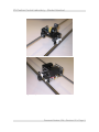
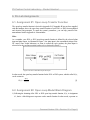
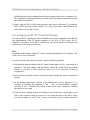
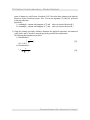
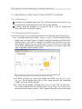
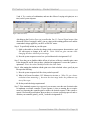
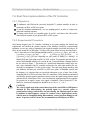
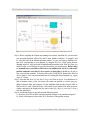
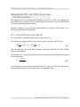
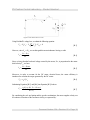
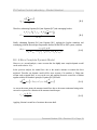
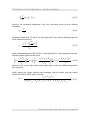
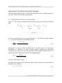
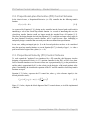
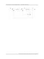
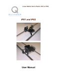
Linear Motion Servo Plants: IP01 or IP02
Linear Experiment #1:
PV Position Control
IP01 and IP02
Student Handout
PV Position Control Laboratory – Student Handout
Table of Contents
1. Objectives.............................................................................................................................1
2. Prerequisites..........................................................................................................................1
3. References.............................................................................................................................1
4. Experimental Setup................................................................................................................2
4.1. Main Components..........................................................................................................2
4.2. Wiring............................................................................................................................2
5. Controller Design Specifications.............................................................................................4
6. Pre-Lab Assignments.............................................................................................................5
6.1. Assignment #1: Open-Loop Transfer Function................................................................5
6.2. Assignment #2: Open-Loop Model Block Diagram.........................................................5
6.3. Assignment #3: PV Controller Design.............................................................................6
7. In-Lab Procedure..................................................................................................................8
7.1. Experimental Setup........................................................................................................8
7.1.1. Check Wiring and Connections...............................................................................8
7.1.2. IP01 or IP02 Configuration....................................................................................8
7.2. Closed-Loop System Actual Requirements.....................................................................8
7.3. Simulation of the Servo Plant with PV Controller.............................................................9
7.3.1. Objectives..............................................................................................................9
7.3.2. Experimental Procedure..........................................................................................9
7.4. Real-Time Implementation of the PV Controller............................................................11
7.4.1. Objectives............................................................................................................11
7.4.2. Experimental Procedure........................................................................................11
8. Post-Lab Questions.............................................................................................................14
Appendix A. Nomenclature......................................................................................................15
Appendix B. IP01 and IP02 Open-Loop Transfer Function......................................................17
B.1. A Simplified Dynamic Model.......................................................................................17
B.2. A More Complete Dynamic Model..............................................................................19
Appendix C. Position Controller Design...................................................................................21
C.1. Standard Closed-Loop System....................................................................................21
C.2. Proportional-plus-Derivative (PD) Control Scheme......................................................22
C.3. Proportional-Velocity (PV) Control Scheme................................................................22
Document Number: 504 w Revision: 02 w Page: i
PV Position Control Laboratory – Student Handout
1. Objectives
In this laboratory session, you will become familiar with the fundamentals of control system design
using PID-types of compensators. The challenge of the present lab is to control the position of
your IP01 or IP02 linear motion servo plant.
At the end of the session, you should know the following:
How to mathematically model the IP01 and IP02 servo plants from first principles in order
to obtain the open-loop transfer function, in the Laplace domain.
How to design and simulate a Proportional-Velocity (PV) position controller to meet the
required design specifications.
How to tune your PV controller gains and their effect on the closed-loop system dynamic
response.
How to implement your controller in real-time and evaluate its actual performance.
2. Prerequisites
To successfully carry out this laboratory, the prerequisites are:
i) To be familiar with your IP01 or IP02 main components (e.g. actuator, sensors), your
power amplifier (e.g. UPM), and your data acquisition card (e.g. MultiQ), as described in
References [1], [2], [3], and [4].
ii) To have successfully completed the pre-laboratory described in Reference [1]. Students are
therefore expected to be familiar in using WinCon to control and monitor the plant in realtime and in designing their controller through Simulink.
iii) To be familiar with the complete wiring of your IP01 or IP02 servo plant, as per dictated in
Reference [2] and carried out in pre-laboratory [1].
3. References
[1] IP01 and IP02 – Linear Experiment #0: Integration with WinCon – Student Handout.
[2] IP01 and IP02 User Manual.
[3] MultiQ User Manual.
[4] Universal Power Module User Manual
[5] WinCon User Manual.
Document Number: 504 w Revision: 02 w Page: 1
PV Position Control Laboratory – Student Handout
4. Experimental Setup
4.1. Main Components
To setup this experiment, the following hardware and software are required:
Power Module:
Quanser UPM 1503 / 2405, or equivalent.
Data Acquisition Board:
Quanser MultiQ PCI / MQ3, or equivalent.
Linear Motion Servo Plant:
2, respectively.
Quanser IP01 or IP02, as shown below in Figures 1 and
Real-Time Control Software: The WinCon-Simulink-RTX configuration, as detailed in
Reference [5], or equivalent.
For a complete and detailed description of the main components comprising this setup, please
refer to the manuals corresponding to your configuration.
4.2. Wiring
To wire up the system, please follow the default wiring procedure for your IP01 or IP02 as fully
described in Reference [2]. When you are confident with your connections, you can power up the
UPM.
Document Number: 504 w Revision: 02 w Page: 2
PV Position Control Laboratory – Student Handout
Figure 1 IP01 System
Figure 2 IP02 System
Document Number: 504 w Revision: 02 w Page: 3
PV Position Control Laboratory – Student Handout
5. Controller Design Specifications
In the present laboratory (i.e. the pre-lab and in-lab sessions), you will design and implement a
control strategy based on the Proportional-Velocity (PV) control scheme, in order for your IP01
or IP02 closed-loop system to satisfy the following performance requirements (which are timedomain specifications):
i) The Percent Overshoot (i.e. PO) should be less than 10%, i.e.:
PO # 10 %
ii) The time to first peak should be 150 ms, i.e.:
tp = 0.15 s
Document Number: 504 w Revision: 02 w Page: 4
PV Position Control Laboratory – Student Handout
6. Pre-Lab Assignments
6.1. Assignment #1: Open-Loop Transfer Function
The open-loop transfer function is derived in Appendix B. If Appendix B has not been supplied
with this handout, derive the open-loop transfer function of your IP01 or IP02 from mechanical
and electrical first principals. To name the system's parameters, you can help yourself of the
nomenclature listed in Appendix A: Nomenclature.
Hint:
As a reminder, your IP01 or IP02 open-loop transfer function is defined by the selected plant
input and plant output. As illustrated in Figure 3, the plant input is the commanded voltage to the
DC motor. Since in this laboratory we want to control the cart's position, the plant output is
selected to be the cart linear position on the rack, as depicted in Figure 3.
Figure 3 The IP01 or IP02 Plant Input and Output
In other words, the open-loop transfer function for the IP01 or IP02 system, which is called G(s),
can be written as:
x( s )
G( s ) =
[1]
Vm( s )
6.2. Assignment #2: Open-Loop Model Block Diagram
1) Following the obtaining of the IP01 or IP02 open-loop transfer function, G(s), in Assignment
#1, derive a block diagram to represent such a transfer function. In other words, represent as
Document Number: 504 w Revision: 02 w Page: 5
PV Position Control Laboratory – Student Handout
individual blocks the basic mechanical and electrical equations that you use to determine G(s).
The resulting block diagram should have an overall closed-loop transfer function identical to the
one found in Assignment #1.
2) Finally, using the IP01 or IP02 model parameter values listed in Reference [2], evaluate the
IP01 or IP02 open-loop transfer function, G(s), that you previously found. Determine the
plant's pole(s), zero(s), and DC gain.
6.3. Assignment #3: PV Controller Design
You will need the PV controller gain values calculated in this pre-lab assignment for the in-lab realtime implementation of the PV position controller for your IP01 or IP02 system. The PV
controller's 2 parameters, i.e. Kp and Kv , will allow the closed-loop system to meet the two time
requirements, as previously set by the user.
Hint:
If supplied with this handout, Appendix C offers a possible implementation of PV controllers. Otherwise, refer to your in-class notes.
In order to determine and calculate Kp and Kv , answer the following questions:
1) Perform block diagram reduction of the PV control scheme applied to G(s), as presented in if
Appendix C has been supplied with this handout. Obtain the overall closed-loop transfer
function of your IP01 or IP02 system by replace G(s) by its expression, as found in
Assignment #1.
2) Extract from the previously obtained closed-loop transfer function the system's characteristic
equation.
3) Fit the obtained characteristic equation to the standard form (seen in Equation [C.3], if
available), by identifying the parameters Tn and .. Thus, you should obtain 2 equations
expressing Tn and . as functions of Kp and Kv as these are the only 2 variables (i.e. controller
parameters) in your system.
4) Using your newly obtained formulae and referring to your in-class notes, what changes to your
IP01 or IP02 response would you expect to see by varying the values of Kp and Kv ? Keep
your answers simple (i.e. will Tn and . increase or decrease?). How would this translate in
Document Number: 504 w Revision: 02 w Page: 6
PV Position Control Laboratory – Student Handout
terms of changes in tp and Percent Overshoot (PO)? Also relate these changes to the physical
behaviour of your closed-loop system. Hint: You can use Equations [23] and [24], presented
in the next subsection.
Specifically:
i) Assuming Kv constant, what happens to Tn and . when you increase/decrease Kp ?
ii) Assuming Kp constant, what happens to Tn and . when you increase/decrease Kv ?
5) Using the formulae previously obtained, determine the analytical expressions and numerical
values for Kp and Kv in order to meet the previously specified time requirements.
The following hint formulae are provided.
i) Hint formula #1:
PO = 100 e
−



ζ π


1 − ζ 2 
ii) Hint formula #2:
π
tp =
ωn 1 − ζ 2
[23]
[24]
Document Number: 504 w Revision: 02 w Page: 7
PV Position Control Laboratory – Student Handout
7. In-Lab Procedure
7.1. Experimental Setup
Even if you don't configure the experimental setup entirely yourself, you should be at least completely familiar with it and understand it. If in doubt, refer to References [1], [2], [3], [4], and/or
[5].
7.1.1. Check Wiring and Connections
The first task upon entering the lab is to ensure that the complete system is wired as fully described
in Reference [2]. You should have become familiar with the complete wiring and connections of
your IP01 or IP02 system during the preparatory session described in Reference [1]. If you are
still unsure of the wiring, please ask for assistance from the Teaching Assistant assigned to the lab.
When you are confident with your connections, you can power up the UPM. You are now ready
to begin the lab.
7.1.2. IP01 or IP02 Configuration
In case you use the IP02 for this laboratory, this experiment is designed for an IP02 cart without
the extra weight on it. However, once a working controller has been tested, the additional mass
can be mounted on top the cart in order to see its effect on the response of the system. As an
extension to the lab, the first PV controller design could be modified in order to account for the
additional weight.
7.2. Closed-Loop System Actual Requirements
As already stated in the pre-lab session, this lab requires you to design a Proportional-plusVelocity (PV) controller to control the position of your IP01 or IP02 cart with the following
performance specifications:
i) The Percent Overshoot should be equal to 10 %:
PO = 10 %, i.e. . = 0.59.
ii) The time to first peak should be 150 ms:
tp = 0.15 s
These specifications are the same as the ones you previously used in the pre-lab session to
calculate the corresponding PV controller gains Kp and Kv .
Document Number: 504 w Revision: 02 w Page: 8
PV Position Control Laboratory – Student Handout
7.3. Simulation of the Servo Plant with PV Controller
7.3.1. Objectives
To simulate with a Simulink diagram your IP01 or IP02 model and to close the servo loop
by implementing a Proportional-plus-Velocity (PV) position controller.
To change, during the simulation, the two gains, Kp and Kv , of the PV controller and
observe the effect on the position response.
7.3.2. Experimental Procedure
If you have not done so yet, you can start-up Matlab now and follow the steps described below:
Step 1. In Simulink, open a model called s_position_pv_ip01_2.mdl. This diagram should be
similar to the one shown in Figure 4. It includes a subsystem containing your IP01 or IP02
modelled plant, as well as the PV controller two feedback loops. In order to be conveniently changed on-the-fly, the two controller gains Kp and Kv are both set by slider gains.
Check that the signal generator block properties are properly set to output a square wave
signal, of amplitude 1 and of frequency 2/3 Hz.
Figure 4 Simulink Diagram used for the Simulation of the PV Control System
Step 2. Before you begin, you must run the Matlab script called setup_lab_ip01_2_position_pv.m. This file initializes all the IP01 or IP02 system parameters and configuration
variables used by the Simulink diagrams.
Step 3. Ensure that the Simulink simulation mode is set to Normal. Click on Simulation |
Start from the Simulink menu bar, and bring up the Position Response (m) scope. As you
monitor the position response, adjust Kp and Kv using the slider gains, as depicted in Figures
Document Number: 504 w Revision: 02 w Page: 9
PV Position Control Laboratory – Student Handout
5 and 6. Try a variety of combinations, and note the effects of varying each gain (one at a
time) on the system response.
Figure 6 Slider Gain for Kv
Figure 5 Slider Gain for Kp
Also bring up the Position Error (m) as well as the Vm (V): Control Signal scopes. Also
discuss the effect of varying Kp and Kv (one at a time) on the resulting position error and the
commanded voltage applied to your IP01 or IP02 DC motor.
Step 4. To specifically include in your lab report:
i) Make a short table to describe the changes in the system response characteristics tp and
PO with respect to changes in Kp and Kv . *Note: Hold one gain constant while
changing the other within the preset range.
ii) Does the system response react to how you had theorized in Assignment #2-4)?
Step 5. Now that you are familiar with the effects of each one of the two controller gains, enter
in the designed Kp and Kv that you have calculated in Assignment #3 to meet the system requirements. *Note: the values should fall within the slider limits.
Step 6. After running the simulation with the gains set to their calculated values, specify in your
lab report the following:
i) Does the system response look like what you had expected?
ii) What is its Percent Overshoot, PO? Measure its rise time, tp . *Hint: To get a better
resolution when measuring t p , decrease the time range under the parameters option of the scope.
iii) Do they match the design requirements?
Step 7. If the simulated response is as expected, you can move on to the next Section in order
to implement a real-time controller. If your response is close to meeting the set requirements, try fine-tuning the controller gains to achieve the desired response. If the system response is far from the specifications, then you have to re-iterate your design process and recalculate your controller gains Kp and Kv , as asked in Assignment #3.
Document Number: 504 w Revision: 02 w Page: 10
PV Position Control Laboratory – Student Handout
7.4. Real-Time Implementation of the PV Controller
7.4.1. Objectives
To implement with WinCon the previously designed PV position controller in order to
command your IP01 or IP02 servo plant.
To run the simulation simultaneously, at every sampling period, in order to compare the
actual and simulated responses.
To change on-the-fly the two controller gains, Kp and Kv , and observe the effect on the
actual position response of your physical IP01 or IP02 system.
7.4.2. Experimental Procedure
After having designed your PV controller, calculated its two gains satisfying the desired time
requirements, and checked the position response of the obtained closed-loop system through
simulation, you are now ready to implement your designed controller in real-time and observe its
effect on your actual IP01 or IP02 plant. To achieve this, please follow the steps described below:
Step 1. Open only one of the following Simulink models: q_position_pv_mqpci_ip01.mdl, or
q_position_pv_mqpci_ip02.mdl,
or
q_position_pv_mq3_ip01.mdl,
or
q_position_pv_mq3_ip02.mdl depending on your model of MultiQ (i.e. MultiQ-3 or
MultiQ-PCI) and if your plant is an IP01 or IP02. Ask the TA assigned to this lab if you are
unsure which Simulink model is to be used in the lab. You should obtain a diagram similar to
the one shown in Figure 7. The model has 2 parallel and independent control loops: one
runs a pure simulation of the PV controller connected to the same plant model as the one
developed in Assignment #2 of the pre-lab section. The other loop directly interfaces with
your hardware and runs your actual IP01 or IP02 servo plant. To familiarize yourself with
the diagram, it is suggested that you open both subsystems to get a better idea of their
composing blocks as well as take note of the I/O connections. Check that the model manual
switch for the position setpoint generation correctly selects the signal coming from the signal
generator block, called Square Wave. Also check that the signal generator block properties
are properly set to output a square wave signal, of amplitude 1 and of frequency 2/3 Hz.
Moreover, your model sampling time should be set to 1 ms, i.e. Ts = 10-3 s.
CAUTION:
The velocity signal used in the control inner-loop of the actual IP01 or IP02 plant is
obtained by first differentiating the position signal (e.g. encoder counts or
potentiometer voltage), and then by low-pass filtering the obtained signal in order
to eliminate its high frequency content. As a matter of fact, high frequency noise,
which is moreover amplified during differentiation, causes long-term damage to the
motor. To protect your DC motor, the recommended cut-off frequency is 50 Hz.
Document Number: 504 w Revision: 02 w Page: 11
PV Position Control Laboratory – Student Handout
Figure 7 Diagram used for the Real-Time Implementation of the PV Controller
Step 2. Before compiling the diagram and running it in real-time with WinCon, you must enter
your previously designed values of Kp and Kv in the Matlab workspace. To assign Kp and
Kv , type their value in the Matlab command window. You are now ready to build the realtime code corresponding to your diagram, by using the WinCon | Build option from the
Simulink menu bar. After successful compilation and download to the WinCon Client, you
should be able to use WinCon Server to run in real-time your actual system. Before doing
so, manually move your IP01 or IP02 cart to the middle of the track (i.e. mid-stroke
position) and make sure that it is free to move on both sides. It should now be safe to
start your real-time controller. To do this, click on the START/STOP button of the WinCon
Server window. Your cart position should now be tracking the desired setpoint (e.g. square
wave of "15mm).
Step 3. Open the sink Meas.(0) and Sim.(2) Resp. in a WinCon Scope. You should now be
able to monitor on-line, as the cart moves, the actual cart position as it tracks your predefined reference input, and compare it to the simulation result produced by the IP01 or
IP02 model. To open a WinCon Scope, click on the Scope button of the WinCon Server
window and choose the display that you want to open (e.g. Meas.(1) and Sim.(2) Resp.)
from the selection list.
Step 4. Specifically discuss in your lab report the following points:
i) How does your IP01 or IP02 cart actual position compare to the simulated response?
ii) Is there a discrepancy in the results? If so, find some of the possible reasons.
Document Number: 504 w Revision: 02 w Page: 12
PV Position Control Laboratory – Student Handout
iii) From the plot of the actual cart position, measure your system tp and PO. Are the values
in agreement with the design specifications? *Hint: You can accurately measure these
parameters by saving the position traces of interest to a M-File (using the WinCon
Scope feature) and making the necessary calculations through Matlab. As a
remark, you could also make these measures directly from the WinCon Scope by
zooming in on the signals, but that would be less convenient to take accurate
measures.
Step 5. Once your results are in agreement with the desired design requirements and your
response looks similar to the one displayed in Figure 8, below, you can move on and begin
your report for this lab. Remember that there is no such thing as a perfect model, and that
your calculated controller gains, Kp and Kv , were based on a theoretical and ideal plant
model.
Figure 8 Actual and Simulated Position Responses to a Square Wave Setpoint
Step 6. However, in order to perfectly meet the chosen design requirements (i.e. tp and PO) of
the closed-loop system, any controller design will usually involve some form of fine-tuning,
which will more than likely be an iterative process. At this point, you should be manually
fine-tuning your Kp and Kv based on your findings above, i.e. from Assignment #3, question
5, and the previous table based on experimental observations in order to ensure your
response matches perfectly the system requirements.
Document Number: 504 w Revision: 02 w Page: 13
PV Position Control Laboratory – Student Handout
8. Post-Lab Questions
1) During the course of this lab, were there any problems or limitations encountered? If so, what
were they and how were you able to overcome them?
2) After completion of this lab, you should be confident in tuning this type of controller to achieve
a desired response. Do you feel this controller can meet any arbitrary system requirement?
Explain.
3) Most controllers of this form also introduce an integral action into the system (PID). Do you
see any benefits to introducing an integral gain in this experiment?
Document Number: 504 w Revision: 02 w Page: 14
PV Position Control Laboratory – Student Handout
Appendix A. Nomenclature
Table A.1, below, provides a complete listing of the symbols and notations used in the IP01 and
IP02 mathematical modelling and controller design presented in this laboratory. The numerical
values of the system parameters can be found in Reference [2].
Symbol
Description
Matlab / Simulink
Notation
Vm
Motor Armature Voltage
Vm
Im
Motor Armature Current
Im
Rm
Motor Armature Resistance
Rm
Lm
Motor Armature Inductance
Lm
Kt
Motor Torque Constant
Kt
0m
Motor Efficiency
Km
Back-ElectroMotive-Force (EMF) Constant
Km
Eemf
Back-EMF Voltage
Eemf
Eff_m
Jm
Rotor Moment of Inertia
Jm
Kg
Planetary Gearbox Gear Ratio
Kg
0g
Planetary Gearbox Efficiency
Eff_g
Mc1
IP01 Cart Mass (Cart Alone)
Mc1
Mc2
IP02 Cart Mass (Cart Alone)
Mc2
Mw
IP02 Cart Weight Mass
Mw
M
Total Mass of the Cart System (i.e. moving parts)
M
Pr
Rack Pitch
Pr
rmp
Motor Pinion Radius
r_mp
Nmp
Motor Pinion Number of Teeth
N_mp
rpp
Position Pinion Radius
r_pp
Npp
Position Pinion Number of Teeth
N_pp
Beq
Equivalent Viscous Damping Coefficient
as seen at the Motor Pinion
Beq
Document Number: 504 w Revision: 02 w Page: 15
PV Position Control Laboratory – Student Handout
Symbol
Description
Tm
Torque Generated by the Motor
Tmp
Torque Applied by the Motor on the Motor Pinion
Fc
Cart Driving Force Produced by the Motor
Fai
Armature Rotational Inertial Force, acting on the Cart
Tai
Armature Inertial Torque, as seen at the Motor Shaft
hm
Motor Shaft Rotation Angle
Tm
Motor Shaft Angular Velocity
Matlab / Simulink
Notation
x
Cart Linear Position
x
PO
Percent Overshoot
PO
tp
Peak Time
tp
t
Continuous Time
s
Laplace Operator
Tn
Undamped Natural Frequency
wn
.
Damping Ratio
zeta
Kp
Proportional Gain
Kp
Kv
Velocity Gain
Kv
Table A.1 IP01 and IP02 Model Nomenclature
Document Number: 504 w Revision: 02 w Page: 16
PV Position Control Laboratory – Student Handout
Appendix B. IP01 and IP02 Open-Loop
Transfer Function
This Appendix derives the mathematical modelling of your IP01 or IP02. The resulting linear
model will provide us with the open-loop transfer function of your IP01 or IP02, which in turn will
be used to design an appropriate controller.
Equation [1] defines G(s), the open-loop transfer function of your IP01 or IP02 system. G(s) is
derived in the following two sub-sections.
B.1. A Simplified Dynamic Model
In a first approach, a simplified dynamic model is used to derive G(s).
We shall begin by applying Newton’s second law of motion to the IP01 or IP02 system:
d
 d2

M  2 x( t )  = Fc ( t ) − Beq  x( t ) 
 dt

 dt

[B.1]
Here, the inertial force due to the motor's armature in rotation is neglected. The cart's Coulomb
friction is also neglected.
The driving force, Fc, generated by the DC motor and acting on the cart through the motor pinion
can be expressed as:
ηg Kg Tm
Fc =
[B.2]
rm p
We now shift over to the electrical components of the DC motor first. Figure B.1 represents the
classic electrical schematic of the armature circuit of a standard DC motor.
Document Number: 504 w Revision: 02 w Page: 17
PV Position Control Laboratory – Student Handout
Figure B.1 DC Motor Electric Circuit
Using Kirchhoff’s voltage law, we obtain the following equation:
∂
Vm − Rm I − Lm  I  − Eemf = 0
m
 ∂t m 
However, since Lm << Rm, we can disregard the motor inductance leaving us with:
Vm − Eemf
Im =
Rm
[B.3]
[B.4]
Since we know that the back-emf voltage created by the motor, Eemf, is proportional to the motor
shaft velocity Tm, we have:
V m − K m ωm
Im =
[B.5]
Rm
Moreover, in order to account for the DC motor electrical losses, the motor efficiency is
introduced to calculate the torque generated by the DC motor:
Tm = ηm Kt Im
[B.6]
Substituting Equations [B.5] and [B.6] into Equation [B.2] leads to:
ηg Kg ηm Kt ( Vm − Km ωm )
Fc =
Rm rm p
[B.7]
By considering the rack and pinion and the gearbox mechanisms, the motor angular velocity can
be written as a function of the cart linear velocity, as expressed by:
Document Number: 504 w Revision: 02 w Page: 18
PV Position Control Laboratory – Student Handout
d
Kg  x( t ) 
 dt

ωm =
rm p
[B.8]
Therefore, substituting Equation [B.8] into Equation [B.7] and rearranging leads to:
d
ηg Kg ηm Kt  Vm r m p − Kg Km  x( t )  

 dt

Fc =
2
Rm rm p
[B.9]
Finally, substituting Equation [B.9] into Equation [B.1], applying the Laplace transform, and
rearranging yields the desired open-loop transfer function for the IP01 or IP02 system, such that:
r m p ηg Kg ηm Kt
G( s ) =
2
2
2
[B.10]
( Rm M rm p s + ηg Kg ηm Kt Km + Beq Rm r m p ) s
B.2. A More Complete Dynamic Model
However, as a second analysis, a more accurate but also slightly more complex dynamic model
can be used to derive G(s).
In the previous analysis, the inertial force due to the motor's armature in rotation has been
neglected. Therefore our dynamic model will be more accurate if it considers it. Taking into
account such an inertial force, as seen at the cart, and applying Newton's second law of motion
together with the D'Alembert's principle, Equation [B.1] becomes:
d
 d2

M  2 x( t )  + Fai ( t ) = Fc ( t ) − Beq  x( t ) 
[B.11]
 dt

 dt

As seen at the motor pinion, the armature inertial force due to the motor rotation and acting on the
cart can be expressed as a function of the armature inertial torque:
ηg Kg Tai
Fai =
[B.12]
rm p
Applying Newton's second law of motion to the motor shaft:
Document Number: 504 w Revision: 02 w Page: 19
PV Position Control Laboratory – Student Handout
 d2

Jm  2 θm ( t )  = Tai( t )
 dt

[B.13]
Moreover, the mechanical configuration of the cart's rack-pinion system gives the following
relationship:
Kg x
θm =
[B.14]
rm p
Substituting Equations [B.13] and [B.14] into Equation [B.12] provides the following expression
for the armature inertial force:
2
 d2

ηg Kg Jm  2 x( t ) 
 dt

[B.15]
Fai =
2
rm p
Finally, substituting Equations [B.9] and [B.15] into Equation [B.11], and rearranging results in the
following dynamic equation for the system:
2
2


ηg Kg Jm   d2
ηg Kg ηm Kt Km  d
η K η K V (t)

 M +
  x( t )  +  B +
  x( t )  = g g m t m
[B.16]
2
 2
  eq
2

Rm rm p

  dt
rm p   dt
 
Rm rm p




Equation [B.16] expresses the system motion with a single second-order differential equation in
the cart position.
Finally, applying the Laplace transform and rearranging yields the desired open-loop transfer
function for the IP01 or IP02 system, such that:
rm p ηg Kg ηm Kt
G( s ) =
2
2
2
2
[B.17]
( ( Rm M r m p + Rm ηg Kg Jm ) s + ηg Kg ηm Kt Km + Beq Rm r m p ) s
Document Number: 504 w Revision: 02 w Page: 20
PV Position Control Laboratory – Student Handout
Appendix C. Position Controller Design
This section deals with the design of a closed-loop controller in order to control the position of
your IP01 or IP02, on a quick and accurate manner.
C.1. Standard Closed-Loop System
Figure C.1, below, depicts a standard closed-loop position control system with a unity feedback
loop:
Figure C.1 Standard Closed-Loop Position Control System
For such a closed-loop system, as represented in Figure C.1, the closed-loop transfer function,
T(s), is given by the following well-established equation:
Gc( s ) G( s )
x( s )
=
xd( s ) 1 + Gc( s ) G( s ) H( s )
[C.1]
Equation [B.17] expresses a plant model that has no zero and 2 poles (i.e. second order
denominator in s). Moreover, in order to design controllers satisfying given performance
requirements, the control theory provides approximate design formulas, which are based, for
quadratic lag systems with no zero, on the following standard equation:
T( s ) =
Kdc ωn
2
s 2 + 2 ζ ωn s + ωn
2
[C.2]
where Kdc is the system's DC gain.
The characteristic equation of the closed-loop transfer function expressed in its standard form by
Equation [C.2] is as follows:
s 2 + 2 ζ ωn s + ωn
2
[C.3]
Document Number: 504 w Revision: 02 w Page: 21
PV Position Control Laboratory – Student Handout
C.2. Proportional-plus-Derivative (PD) Control Scheme
In the classical sense, a Proportional-Derivative (i.e. PD) controller has the following transfer
function:
Gc( s ) = Kp + Kd s
[C.4]
As expressed by Equation [C.4], placing such a controller into the forward path would result in
introducing a zero in the closed-loop transfer function. As a result of introducing this zero, the
closed-loop transfer function would no longer match the standard form of Equation [C.2].
Therefore, the design formulae derived from Equation [C.2] would also no longer exactly apply to
the thus obtained closed-loop transfer function, and it would become more challenging to
analytically design a controller that can exactly meet the user-defined time specifications.
In our case, adding an integral gain (i.e. I) to the forward path does not have to be considered
since the open-loop transfer function, as seen in Equation [B.17], is already of type 1, i.e. it has a
pole located at the origin of the s-plane (i.e. s = 0).
C.3. Proportional-Velocity (PV) Control Scheme
To work around the "undesired" zero introduced by a PD controller, this laboratory involves
designing a Proportional-Velocity (i.e. PV) position controller for the IP01 or IP02 servo plant.
Such a controller introduces two corrective terms: one is proportional (by Kp ) to the position error
and the other is proportional (by Kv ) to the velocity (or the derivative of the actual position) of the
plant. Coincidentally, the characteristic equations of the PV and PD controller closed loop transfer
functions are equal.
Equation [C.5], below, expresses the PV control law, where xd is the reference signal (i.e. the
desired position to track):
d
Vm( t ) = Kp ( xd( t ) − x( t ) ) − Kv  x( t ) 
[C.5]
 dt

Figure C.2, below, depicts the block diagram of the PV control scheme, as it will be implemented
in this lab:
Document Number: 504 w Revision: 02 w Page: 22
PV Position Control Laboratory – Student Handout
Figure C.2 Block Diagram of the PV Control Scheme
Document Number: 504 w Revision: 02 w Page: 23