1
ESO Phase 3 Data Release Description Data Collection Release Number Data Provider Document Date Document version Document Author On-line version GIRAFFE_MEDUSA 1 ESO, Quality Control Group <20.04.2015> 1.0 Reinhard Hanuschik http://www.eso.org/qc/PHOENIX/GIRAFFE/processing.html Abstract This is the release of reduced 1D spectra from the FLAMES/GIRAFFE1 spectrograph, taken in the MEDUSA mode. This is the most frequently used multi-object spectroscopy mode of GIRAFFE, as opposed to its two IFU modes. FLAMES is the multi-object, intermediate and high resolution spectrograph of the VLT, having two components: GIRAFFE and UVES. The GIRAFFE spectrograph allows the observation of up to 130 targets in one shot with intermediate resolution. This release is an open stream release, it includes so far observed GIRAFFE data and will be continued into the future operational lifetime. The data content will grow with time as new data are being acquired and processed (approximately with monthly cadence and with a short delay of 1 or 2 months). The processing scheme is as homogeneous as possible. The currently available release covers all GIRAFFE MEDUSA data starting from 2005-06-01 until 2014-12-31. The earlier data for GIRAFFE (covering the period from begin of operations in 2003-04 until May 2005) will be supplemented as soon as possible. The data have been reduced with the GIRAFFE pipeline, version giraf-2.13.2 and higher. The data have most of their instrument signature removed: they have been de-biased, flat-fielded, extracted, and wavelength-calibrated. Their wavelength scale has been corrected to the heliocentric reference system. The processing is performed by the Quality Control Group in an automated process. The pipeline processing uses the archived, closest-in-time, quality-controlled, and certified master calibrations. It is important to note that the reduction process itself is automatic, while the quality assessment and certification of the master calibrations is human-supervised. The pipeline products come in the ESO 1D standard binary table 2, along with a set of ancillary files. The data products cover many different science cases (defined by their parent programmes, in the case of GIRAFFE several hundreds). The data format follows the ESO 1D spectroscopic standard 2 for science data products. Each spectrum is a multi-column binary table. There are N product files for each input science raw file, where N corresponds to the number of science fibres. N can be as high as 130 (the number of science or sky fibres in each Medusa fibre system)3. http://www.eso.org/sci/facilities/paranal/instruments/flames.html http://www.eso.org/sci/observing/phase3/p3sdpstd.pdf 3 Five more fibres can be used for the simultaneous calibration, so that the total number of fibres is 135. 1 2 1 This data release offers science-grade data products, with the instrumental signature removed to a large extent. The spectra come with error estimates and a signal-to-noise column (SNR), and with a list of known shortcomings. They are considered to be ready for scientific analysis. They are expected to be useful for any kind of medium resolution spectroscopic research, including abundance and line profile studies, and radial velocity studies. There has been no attempt to correct for sky background. We provide the signal from all SKY fibres but leave it to the user to select the appropriate ones for a given target. See more under ‘Data reduction and calibration’. Disclaimer. Data have been pipeline-processed with the best available calibration data. However, please note that the adopted reduction strategy may not be optimal for the original scientific purpose of the observations, nor for the scientific goal of the archive user. You may also want to consult the on-line version of this documentation4 which is a living document and has further useful links. Release Content The GIRAFFE_MEDUSA release is a stream release. The overall data content is not fixed but grows with time as new data are being acquired and processed. The data are tagged "GIRAFFE_MEDUSA" in the ESO archive user interface5. The first data have been published under GIRAFFE_MEDUSA in April 2015, with GIRAFFE data from June 2005 until the end of 2014. The earlier Medusa data from GIRAFFE will be published soon. New data taken in 2015 and beyond are being added at roughly monthly intervals and with a delay of 1 or 2 months, when all master calibrations for the corresponding time interval are available. Data Selection Data selection is rule-based. The following rules apply: instrument=GIRAFFE; observing technique (FITS key DPR.TECH) = MOS, INS.MODE=MED, INS.SLIT.NAME=Medusa1 or Medusa2 category (DPR.CATG) = SCIENCE; type (DPR.TYPE) = OBJECT,OzPoz or OBJECT,SimCal. No selection is made on the basis of the observing mode (visitor or service), nor on settings. Settings. GIRAFFE MOS settings are defined by the combination of INS.SLIT.NAME (Medusa1 or Medusa2) which is actually the fibre system; central wavelength (in nm); and grating name (HR or LR). For some central wavelengths, two different order separation filters are offered for the observations. In those cases the setting is made unique by appending a letter A or B (e.g., H525.8B). In all other cases the setting is marked as L543.1 or H665.0. The setting is stored in the FITS key INS.EXPMODE. Input files. In all cases each spectral data product is based on a single input raw file. We did 4 5 http://www.eso.org/qc/PHOENIX/GIRAFFE/processing.html http://archive.eso.org/wdb/wdb/adp/phase3_spectral/form 2 not combine multiple exposures within an OB 6, no matter if from the same night or from different nights. We did not combine multiple exposures with different wavelength setups within the same OB. SimCal vs. OzPoz. For the DPR.TYPE, two different values exist: OBJECT,OzPoz: this is the classical GIRAFFE Medusa observation, using the OzPoz fibre positioner on plate 1 (with the fibre system Medusa1) or plate 2 (Medusa2). Both are logically equivalent (one plate is used to configure the next OB while the other one is still observing) but need their own fibre and calibration system and are therefore always distinguished. An OzPoz observation has always been processed into a set of products, unless, very rarely, the processing failed or an OzPoz observation has no science fibre configured. OBJECT,SimCal: this is also a GIRAFFE Medusa observation taken with OzPoz, with additional simultaneous arclamp calibrations illuminating the 5 SimCal fibres. The purpose of this is to provide a reference for incremental shifts against the daytime arclamp calibrations. This observing mode is chosen for high-precision radial-velocity studies. Beyond about 700 nm there are some very strong arc lines which easily saturate and contaminate the signal of neighbour fibres. Therefore many observers have designed their OBs such that they contain multiple exposures, with one or more short SIMCAL observations and one or more longer OZPOZ observations, taken with the same fibre configuration and setting. The short SIMCAL observations are designed to deliver the signal of the SIMCAL lamp (5 fibres) without saturation, but the signal of the science fibres is just noise. These SIMCAL data can be considered as calibrations. Unfortunately they are not formally marked as such but still carry the DPR.CATG value SCIENCE. Below about 700 nm, there exist many SIMCAL observations with long exposure times, in settings where the SIMCAL emission lines do not saturate. These data are clearly science-type observations, with the SIMCAL fibres adding RV precision. We have made an attempt to recognize this complex pattern empirically. For those OBs with an OZPOZ observation and (one or more) SIMCAL observations, we have always treated the SIMCAL observations as calibration-type and attached them to the corresponding OZPOZ products, with their names starting with GI_SSIM. With this delivery pattern, we intend to avoid offering pseudo-science products from the short SIMCAL exposures which would actually contain only noise in the science fibres. A more complex handling is required for stand-alone SIMCAL observations. These come typically as single observations with longer exposure times, but some observers (typical for Visitor Mode) have designed special OBs with complex SIMCAL observation patterns (several settings combining short and long exposure times). With the goal in mind to distinguish calibrationtype and science-type SIMCAL data, we have normally rejected stand-alone SIMCAL observations, unless the following criteria apply: 6 Exposure time is longer than 120 sec. Wavelength setting is not contained in a list of configured rejection values that mostly contain the red settings beyond 700 nm (but 881.7 is accepted). OB = Observing block, a single pointing on the sky and the fundamental unit of the VLT observations. 3 The threshold of 120 sec is empirical, almost all calibration-type SIMCALs are shorter or equal. This schema works well to save the science-type SIMCAL products and avoid calibration-type products containing only noise. In Table 1 we have collected the most typical patterns we have seen in GIRAFFE Medusa OBs. Table 1: Possible OzPoz/SimCal combinations and their data product setup within the same OB: DPR.TYPE … OZPOZ (only) OZPOZ | OZPOZ SIMCAL (only) SIMCAL | OZPOZ SIMCAL | OZPOZ | SIMCAL OZPOZ | OZPOZ | SIMCAL SIMCAL60 | SIMCAL30 | SIMCAL10 | OZPOZ resulting in … classical set of products, no SIMCAL attached two sets of products, no stacking if exptime is longer than 120 sec: accepted as SCIENCE if central wavelength shorter than about 700nm (with a few exceptions), otherwise not OZPOZ products, with 1 SIMCAL attached OZPOZ products, with 2 SIMCALs attached both OZPOZ get their own product dataset, with the SIMCAL file attached multiple SIMCALs with short exposure times: all attached to OZPOZ (with SIMCAL10 meaning 10 sec exposure time) There are very rarely false suppressions, with a SIMCAL file intended by the PI as science file. This could have happened for a SIMCAL short exposure (less than 120 sec) taken in the settings beyond 700nm. In the few cases which we discovered and checked these were “exotic” observations, like 1 science fibre only with lots of sky fibres. These might also have been aborted exposures with the SIMCAL lamp erroneously off. There are very rare cases when an OZPOZ file did not contain a single SCIENCE fibre (only SKY fibres). In that case no product was created. General processing pattern. We have processed only those Medusa science data for which certified master calibrations exist in the archive. These master calibrations exist normally at daily frequency. They were all processed by the Quality Control Group, close to the date of acquisition, in order to provide quality feedback to the Observatory. All master calibrations used here were certified, meaning checked for quality and proper registration of instrument effects. In general, the master calibrations were processed with different (earlier) pipeline versions than the science data in this release. The most significant change in the GIRAFFE pipeline was related to the replacement of the old CCD by the new CCD in 2008-05. While data from the old CCD often have a glow induced by a diode, the new CCD does not have this artefact. The old CCD also had two bad columns while the new CCD has no such imperfections. The reduction strategy required the subtraction of a scaled master dark for the old CCD, and the masking of the bad columns with a bad pixel mask. Both calibration steps are not required for the new CCD. See “Master calibrations” below for a discussion of the main differences. Science data with the OBS.PROG.ID starting with 60. or 060. have been de-selected, considering them as test data. Data taken at daytime (with obviously wrong ‘SCIENCE’ tag) have been ignored. Otherwise the header tag ‘SCIENCE’ has been blindly accepted from the raw data (originally defined by the PI), thus including sometimes standard stars intended by the observer for use as calibrators for flux or radial velocity. Please check the OBJECT header key for 4 such cases. It is likely that most of the products with just one science fibre fall into that regime. Also, there are rare cases when test observations were executed under the SCIENCE label. Some very short exposures with no signal fall into that category but have not been suppressed. For a discussion of the science vs calibration property of the SIMCAL data see the above section. GIRAFFE does not foresee flux calibration for the Medusa mode. The data come extracted and wavelength-calibrated but with no flux calibration. There is no raw science data selection based on quality. Likewise, we have not considered OB grades7: the observations might have any grade between A and D (if taken in Service Mode, SM), or X (in Visitor Mode, VM). The availability, or non-availability, of a particular file in this release does not infer a claim about the data quality. Find the OB grade, and OB comments if any, in the attached ancillary README file. Release Notes Pipeline Description The data reduction uses the standard GIRAFFE pipeline recipe giscience. Find its description in the Pipeline User Manual8. Find the pipeline version used for processing in the header of the product file, under “HIERARCH ESO PRO REC1 PIPE ID”. The version for the initial dataset (the historical batch from 2005-06-01 until 2014-12-31) was giraf/2.13.2. For the recipe parameters, almost any are set to the pipeline defaults. The only exceptions are: --bsremove-method=PROFILE+CURVE (in order to take into account the structure of the master bias which has some curvature); --bsremove-yorder=5 (the polynomial coefficient for the curvature fit); --flat-apply=TRUE; - the technical parameters required to make a product compliant with the ESO Data Product Standard9. Find more details in the Pipeline User Manual8, section 9.6 (for issue 6). Information about the GIRAFFE pipeline (including downloads and manual) can be found under the URL http://www.eso.org/sci/software/pipelines/. The QC pages10 contain further information about the GIRAFFE data, their reduction and the pipeline recipes. 7 As given by the observatory staff to assess the match with user-defined constraints, for SM data. Under the GIRAFFE link in http://www.eso.org/sci/software/pipelines/. 9 Namely: generate-SDP-format=TRUE (to generate the output format of the spectra), and dummyassociation-keys=4 for the technical ASSOC/ASSON keys. 10 http://www.eso.org/qc/GIRAFFE/pipeline/pipe_gen.html 8 5 Data Reduction and Calibration Reduction steps. Each GIRAFFE Medusa frame is reduced individually. The main reduction steps are the following: Note: The input spectrum is bias-corrected, using a polynomial fit to the provided master bias. For data earlier taken earlier than 2008-05 (with the old CCD), the closest-in-time master dark is scaled for exposure time and subtracted. This helps removing the glow in the upper right part of the CCD. The master darks have been taken about monthly and are associated closest-in-time to the science frame. No such correction is needed for data taken after that date (new CCD). For the same date range, the bad-pixel mask is applied, to suppress the wrong and meaningless signal in the two bad columns. No such correction is needed for data taken after that date (new CCD). Using the localization and fibre-width tables (coming together with the master flat as solution from the gimasterflat recipe), the science spectrum is extracted. We have used the default (SUM) extraction. The optimal extraction has issues with high-frequency oscillations, and would also have required the creation of new master flats. The master flat is used to correct for fringing, pixel-to-pixel gain variations and fibreto-fibre transmission. Finally the dispersion solution is used to apply the wavelength calibration, and the resampling to a wavelength grid. For SIMCAL data, the provided line-mask is used to cross-correlate with the obtained wavelength solution, in order to derive a residual wavelength drift. The resulting differential shifts are applied to the SIMCAL data and are written into the binary output table of the SIMCAL observation. The individual spectra have been shifted to the heliocentric RV system, using the barycentric, heliocentric and geocentric corrections. The ancillary 2D products are not RV corrected (since the RV shift has subtle differences from fibre to fibre). In the cases where the observer has chosen to have separate OZPOZ and SIMCAL observations, the shift as derived in the SIMCAL observation(s) has not been applied to the OZPOZ data. No SKY subtraction has been applied. Instead, all fibres with a sky signal (as defined by the observer) are collected in the associated MOSSKY file (with name GI_SSKY). It is generally not possible for an automatic reduction process to select the appropriate sky signals. Many observers configure their sky fibres across the entire field of view. The user may want to use a mean, a 2D fit, or fine-tuned strategies depending on fibre location. 6 Master Calibrations used for data reduction11 Table 2. Set of master calibrations used for data reduction Type (pro.catg) MASTER_BIAS name (first part) GI_MBIA Mandatory*/ optional optional MASTER_DARK GI_MDRK optional (but always provided for data before 2008-04) FF_LOCWIDTH, FF_LOCCENTROID, FF_EXTSPECTRA, FF_EXTERRORS GI_PLOC, GI_PLOW, GI_PFEX, GI_PFEE mandatory DISPERSION_SOLUTION GI_PDIS mandatory BAD_PIXEL_MAP GI_PBPX LINE_MASK GI_GMSK Optional (but always provided for data before 2008-04) Optional GRATING_TABLE SLIT_GEOMETRY_SETUP GI_GRAT GI_GSGS mandatory mandatory content created from 5 raw bias frames; removes bias level and bias structure. created from 3 raw dark frames; removes or reduces diode glow (dark current is negligible). tables derived from flat field (3 input flat frames), with localization information for each fibre, and with extracted signal for pixel-to-pixel gain correction (incl. error) Dispersion table derived from single arc frame Static bad pixel map, corrects for bad columns Static line mask, required for cross-correlation of SIMCAL data Static grating table Static slit geometry, describing fibre arrangement in the slit * Mandatory: if missing, pipeline would fail; optional: not strictly required but always provided for science data products Wavelength scale. The GIRAFFE Medusa products are wavelength calibrated. The wavelength scale is heliocentric. The correction values that have been applied are stored in the header (HELICORR, BARICORR, GEOCORR, in km/s). Telluric absorption. No correction for telluric absorption lines has been applied. Generally telluric correction is not a major concern for GIRAFFE observations. No dedicated telluric standard star observations exist. Users may want to visit the ESO skytools web page12 for appropriate tools. Bad pixel map. We have used the same bad pixel map throughout the epoch of the old CCD. This is generally a reasonable strategy but we cannot exclude that in certain cases a custom bad pixel map would mask the affected bad columns in a better way. We have marked the potentially affected data products with a quality flag (see below). 11 12 Please check Sects. 8 and 9 of the Pipeline User Manual for the description of calibration data. http://www.eso.org/sci/software/pipelines/skytools/ 7 Master darks. We have reduced the spectra with closest-in-time master darks (intended to correct for the diode glow on the old CCD) selected from a pool of master darks taken at about monthly intervals. In individual cases they still do not match the prevailing conditions for the science data very well, since the glow level was variable. We have marked the potentially affected spectra with a quality flag (see below). Master calibration names and recipe parameters used for reduction. The product header contains a list of all used master calibrations, look for keys “HIERARCH ESO PRO REC1 CAL<n> NAME” and “... CATG”, with the index n. The used pipeline parameters and their values are listed as “HIERARCH ESO PRO REC1 PARAM<n> NAME” and “... VALUE”. Products. The final GIRAFFE science data product in the binary spectroscopic data format combines information from the following 2D pipeline products: 2D extracted spectrum (de-biassed and if applicable dark-corrected, flat-fielded, extracted, wavelength-calibrated, rebinned): all fibres combined (SCIENCE, SKY, SIMCAL if used). Corresponding 2D error file. The spectra are extracted by the pipeline from the 2D pipeline product, one spectrum per SCIENCE fibre. Each spectrum is a binary FITS table file, with the wavelength values as first column, then the extracted signal for the corresponding fibre, the corresponding error, and the SNR as ratio of the signal and the error (provided for convenience, it does not contain new information). The following additional files are delivered as ancillary FITS files: The entire 2D extracted spectrum is delivered for quality checks. If SKY fibres exist, there is an extraction from the 2D file of all SKY fibres, with the product category ‘ANCILLARY_MOSSKY’. If existing, the attached SIMCAL observations are added (see ‘File Structure’ below). Finally, there are two overview plots added as ancillary non-FITS files to each product spectrum. One is a QC report, applicable to the whole set of products from the parent raw file, and one is a preview plot of the spectrum. The spectra contain some header keywords that have been added by the pipeline. They are listed in Table 3: 8 Table 3. FITS keywords added by the pipeline parameter values OB related information: SM_VM SM or VM OB_GRADE A/B/C/D; X OB_COMMn Free text QC related information: QCFLAG e.g. 000000100 QC_COMMENT Free text meaning Data taken in Service Mode or Visitor Mode; VM data are less constrained in terms of OB properties; they have no user constraints defined and therefore no OB grades Immediate grade given by night astronomer, considering ambient conditions checked against user constraints (VM data are formally graded X meaning ‘unknown’) Any optional comments added by the night astronomer, together with the approximate UT hh:mm (truncated after 200 characters). [Note that OBs might have been executed several times during the night, with or without comments. In those cases the user should always carefully check that the listed comment applies to the data product with the closest previous timestamp.] QC flag composed of 9 bits, see Table 4. Automatically added comment if a quality issue is discovered by the processing system (human-provided comments also exist but are very rare): SCIENCE SIMCAL (a stand-alone SIMCAL observation processed as SCIENCE) No SKY fibres defined More than 1000 pixels saturated Rejected or failed processing. The GIRAFFE pipeline evaluates the binary OZPOZ table (FITS extension of the raw file), column TYPE, value M (for “Medusa science”). The TYPE values (could also be S for “sky”) are user-designed. Products are created only for fibre type M. If a user has not assigned a science fibre (by mistake or by intent), there will be no product. If no certified master calibrations exist, no processing can be done. This was a very rare event. In cases of quality issues (high number of saturated pixels, time or temperature mismatch of calibrations) we have flagged those data in the QC flag but leave the final assessment to the user (see Section ‘Data Quality’). Data Quality Master calibrations. All used master calibrations have been quality-reviewed and certified at the time of acquisition, as part of the closed QC loop with the Observatory which also includes trending13. As part of the certification process there is always a scoring to bring non-compliant behavior of the calibrations to the attention of the QC scientist. All these cases have been handled as part of the certification procedure. Hence there is reasonable evidence that the master calibrations catch all instrument properties, as relevant for the reduction, correctly and completely. The most important parameters for the quality of the products are the SNR of the master flats, and the rms of the dispersion solution. The SNR of the master flats was always high enough 13 Check out for more under the GIRAFFE link of http://www.eso.org/qc/ALL/daily_qc1.html. 9 (both for the old and the new CCD) to be dominated by the fixed-pattern (gain) noise, which is important to not compromise the SNR of the science data. The rms of the wavelength dispersion (Figure 1) was slightly higher in the first few years than later, due to a slight degradation of the focus over the years. This effect is entirely instrumental and not due to evolving quality of the pipeline. Actually the quality of the master calibrations has been very stable over the years14. SNR. There is a column “SNR” in the spectral product that is calculated from the signal and the corresponding error. It has no independent information but is calculated from the two columns FLUX_REDUCED and ERROR_REDUCED and is provided for convenience. Its mean value across the spectrum is written into the header as key SNR. Figure 1. Performance of the RMS of the dispersion solution for the reference setting Medusa1 H525.8B. This Health Check plot is based on ARCLAMP calibrations taken every 3rd day. SPEC_RES. The resolving power is derived from the arclamp calibrations for the same setting as the science data. The actual resolution of the science data has not been measured directly but very likely is the same as for the arclamp calibration, since all spatial information (position, FWHM of the source due to seeing) is lost due to scrambling within the fibre. The header key SPEC_RES has been filled from a look-up table containing mean values for each setting, derived from the HC data. The stability of SPEC_RES is illustrated in Figure 2 for a reference setting. See http://www.eso.org/qc/GIRAFFE/reports/HEALTH/trend_report_ARC_RMS_HC.html for the trending plots; click “FULL” for the entire history. 14 10 Figure 2. Resolving power measured from ARCLAMP frames for the reference setting Medusa1 H525.8B. QC flag. The header key “QCFLAG” in the GIRAFFE products contains a quality flag. It is composed of nine binary bits (Table 4). For each bit, the value 0 means “no concern”. The final QC flag is composed of all components. For instance, 000000000 is a pristine product. 010000000 or 100000000 or 110000000 describe products that have been processed with an ARCLAMP calibration product that deviates in ambient temperature, or time, by more than a nominal value (1.5 degrees or 1 day). The motivation for this comes from the temperature sensitivity of the grating which moves slightly in both cross-dispersion and dispersion direction with temperature15. These thermal drifts are minimized by the daily calibration plan which foresees these calibrations to be taken right after the science data, in daytime. Occasionally this rule cannot be satisfied, and the score #2 (deltaTime) flags this. This occurs only rarely, and is likely to be uncritical, but in principle the wavelength scale could be less accurate in those cases. The QC flag 001000000 marks an issue with the number of saturated pixels. In practise, saturated pixels are not intrinsic to the spectrum but arise from cosmics, or sky emission lines. Flag #4 is for process control only. Flag #5 indicates if no SKY fibre is available (or not marked as such by the observer). In practice this happens rarely. Flag #6, if 0, marks an OZPOZ file that has attached SIMCAL file(s). Although it is very normal for an OZPOZ file to have no SIMCAL file attached, it was decided to encode flag #6 in this way since with an attached SIMCAL, the observation can have in principle the highest possible wavelength accuracy. It follows that a value 1 does not imply any issue with the data. The value 0 is only possible for an OZPOZ file. 15 Check out http://www.eso.org/qc/GIRAFFE/reports/HEALTH/trend_report_STABILITY_HC.html for more. 11 Bit #1 –deltaTemp #2 - deltaTime #3 – saturated pixels #4 – number of science fibres #5 – number of sky fibres #6 – flag for simcal attached Content (if YES, value is 0, otherwise 1) abs(deltaTemp) below 1.5 degree? (deltaTemp=difference between ambient temperature for science and for arclamp calibration) abs(deltaTime) below 1 day? (deltaTime=difference between acquisition time of science and arclamp calibration) number of saturated pixels below 1000? ≥ 10? Motivation ≥1 flag cases where no sky fibre is available attached SIMCAL file(s) exist(s)? 0 is possible for OZPOZ files only; if attached SIMCAL file exists, accuracy of wavelength scale can be checked and corrected to highest possible level if yes, that product does not suffer from contamination by SIMCAL fibre signal; if no (value=1), be aware of possible contamination if no (value=1), be careful with the signal, it could have wrong offsets if no (value=1), be careful with the signal; the master_dark could have over/undercorrected the glow #7 – OBJECT type OBJECT,OzPoz? #8 – bad column flag product unaffected by bad column (old CCD)? product unaffected by CCD glow? #9 – glow flag increased probability of calibration mismatches between science and arclamp calibrations (rarely violated) usually daytime calibrations come within 0.5 days; if more than a day difference, probability is higher that shifts have occurred for arclamp data (impacts wavelength scale) (rarely violated) not critical if due to cosmics; never due to saturation of larger spectral portions relevant for process control only Table 4. QC flags. Flags #1-#7 apply to all products from the same raw file in the same way. Flags #8 and #9 apply to individual fibres (could be 1 for some products and 0 for others), depending on their localization on the CCD. These flags have a meaning only for data before 2008-05 (old CCD). Flag #7, if 0, marks that the file itself is from an OZPOZ observation. The SIMCAL fibre signal in the neighbourhood of emission lines could in principle cause some cross-talk, or even saturation in extreme cases, for the SCIENCE fibres. Therefore a SIMCAL product is always marked by the value 1, to make the user aware of potential issues16. In combination, the flags #6 and #7 can have the values 000000000 (OZPOZ file, with SIMCAL file attached); 000001000 (OZPOZ file, no SIMCAL attached); or 000011000 (SIMCAL science file). Of course all other flags could be 0 or 1. While flags #1-#7 apply to all products from the same parent raw file in the same way, flags #8 and #9 may vary among them. They are applicable to data from the old CCD. Flag #8 marks products from a fibre that is affected by the bad columns, and flag #9 is for fibres that are affected by the CCD glow. Therefore some observers have chosen to have a long OZPOZ exposure and one or more short SIMCAL exposures in the same setting and OB. 16 12 Science products. The pipeline processing of the science data is done automatically, with some internal quality control, monitoring: the quality of the associations of calibration data (checking that the master calibrations used are applicable to the science data, flagged in the QCFLAG); flags for the number of saturated pixels, and for potential issues from the data reduction (see above, Table 4); on-demand QC reports and quick-look overviews. This information has largely been used to improve and fine-tune the reduction process. An individual one-by-one inspection of the products has not been done. The QC reports and spectral overviews are delivered along with the spectral products. Previews. The preview plots have been originally developed as quick-look plots for process quality control. It was felt that they might also be useful to the archive user. They are delivered as ancillary files along with the products. There are two plots: 1. the main QC plot (Figure 3), one per dataset (the same for all products from the same raw file); 2. the preview plot (Figure 4), one per product. Figure 3. Main QC plot of the whole dataset, featuring: boxes 1 and 2 – crosscuts from the raw file; box 3: SNR vs. counts for all fibres (SCIENCE in black, SKY in blue, brightest SCIENCE in red); box 4: histograms for 2D product, focus is on the region around the background, counts are on a logarithmic scale; histogram for raw file, focus is on region around saturation, 65000 ADUs; boxes 5 – spectral overviews, top: all available sky spectra plotted in blue; middle: signal from brightest fibre, in blue the last sky fibre; bottom: SNR plot for brightest fibre; at bottom: a set of QC parameters applicable to the parent raw file and the 2D products, including the flag for attached SIMCAL (Y/N), number of fibres (total, science, sky, simcal), spectral coordinates in nm, resolving power, deltaTime and deltaTemp values, number of saturated pixels, and SNR of brightest spectrum. 13 Process quality control. The quality of the data reduction is monitored with quality control (QC) parameters, which are stored in a database. The database is publicly accessible through a browser and a plotter interface 17. QC parameters are used to monitor the reduction quality. The most important check is the “SNR versus signal” control plot (the signal being expressed as the mean across the entire reduced spectrum, and the SNR being the mean over the entire spectral range). Figure 5 shows data points from the reference setting H665.0 which has been selected because it has a rich selection of products. Only data for the brightest fibre are displayed, to avoid confusion. Two data sets are displayed: one (in red) is for the data from 2014 only, the other (in blue) is for products from 2009-09 on. (From that date on, the pipeline version giraf/2.8 was used for the calibration data processing. Previous versions had a bug with the computation of the error and hence with the SNR.) Figure 4. Preview plot of the spectral product, featuring: panel 1a – all sky fibres (same plot as before); 1b – the spectrum, plus the last sky fibre for comparison; 1c – the SNR of the spectrum; also displayed: the SNR plot for all spectra of the same raw file, with this one highlighted in red. At bottom: a set of QC parameters applicable to the spectrum, including the score bits (QC flag), the flag for attached SIMCAL (Y/N), mean flux and SNR, resolving power, deltaTime and deltaTemp values, and object properties like FPS (fibre index), object name, and user defined magnitude. 17 Browser: http://archive.eso.org/qc1/qc1_cgi?action=qc1_browse_table&table=giraffe_science_public Plotter: http://archive.eso.org/qc1/qc1_cgi?action=qc1_plot_table&table=giraffe_science_public 14 Figure 5. SNR vs signal. All data points are from the same setting, H665.0, both Medusa fibre systems. Only the signal from the brightest fibre is displayed here. Data points in red refer to the year 2014. The other data points cover the range 2009-09 and later. This figure shows the square-root law expected if the data quality is limited by photon shot noise. Out to SNR values as high as 400 there is no flattening observed, as one might otherwise expect if the SNR is limited by imperfect data reduction, e.g. by imperfect flat-fielding. Another effect is visible in this figure, namely the stability of the reduction scheme and of the instrument. There is no significant difference between the entire dataset displayed in this figure (blue points) and the data from 2014 only (red points). The highest SNR found so far is in excess of 700 (Figure 6). Figure 6. All Medusa1, HR data (brightest fibre), data from 2010 until end of 2014. Maximum SNR found is in excess of 700. 15 Known features and issues This list might evolve with time. Issues. Old CCD (data acquired until 2008-04), dispersion solution. All care has been applied to process the data with the proper master calibrations. Since visual checks were unaffordable, we cannot entirely exclude that there are minor differential shifts across the fibre dispersion solution. We recommend to inspect the GI_SRBS file with an image browser. Any sky emission or absorption lines should be perfectly straight across all fibres. Old CCD, bad columns. The old CCD has two bad columns that cover part of the CCD and affect mostly the signal in fibre FPS24. Depending on the spectral format, the impact may be strong or negligible. A bad pixel table has been used to mask out these two bad columns. But the extent and strength of the artefact (non-linear or negative counts) may have been variable and hence the masking imperfect. We have marked those spectra with the bad column flag #8. Please check those spectra carefully, their count level might be off (with the shape of spectral features being still correct). Old CCD, glow correction. With the monthly master darks, the strength of the glow may have been over/under-subtracted occasionally. The affected area is the upper right part of the CCD which translates into a fibre index between approximately FPS109 and FPS124 and affects about the last quarter of the spectrum at most. Such data are marked in the previews and scores, check your preview. If the slope is flat, all is ok. If there is an upwards or downwards slope, the spectrum is affected by the improper glow correction. The glow has low spatial frequencies only, hence neither the shape of spectral lines nor their RV are affected. If a proper slope is important, correcting with a low-frequency fit to the slope is likely to be sufficient. In more severe cases a full reprocessing is required, with appropriate scaling of master dark. Old CCD, fringing in red setups. The old CCD has a significant fringing in the red settings. The correction by the flat-fielding is very good, as is visible in Figure 7. New CCD (since 2008-05). For the period 2011-11-20 until 2011-12-22, and the fibre system Medusa1, one fibre (FPS27) was enabled that was never enabled before or after. There is no precise configuration available for the pipeline to process that fibre, and it was decided to not process those datasets into data products. A total of 13 input raw GIRAFFE files is affected. Medusa2 data are not affected by this issue, and their products have been processed. Figure 7. The lower panel (the SNR plot from the spectral preview plot) shows the fringing pattern typical of the red settings observed with the old CCD. The master flat shows exactly the same pattern which then cancels out in the extracted signal (top panel). 16 General (old or new CCD). Last fibre(s). The pipeline extracts only fibre signals falling entirely onto the chip, meaning out to FPS135 at most. Any signal in incomplete fibres is ignored. Sky/science type in FPOSS. The type is configured by the observer. The pipeline extracts spectra for fibres assigned type “M” (science), and collects fibres assigned type “S” into the ANCILLARY_MOSSKY file. If the observer has confused sky and science in one or more fibres, the pipeline cannot correct for this. See Figure 8 for a possible example. Possibly wrong OB grades in FITS keywords. If in Service Mode an OB is executed twice (or in general more than once) during the same night, this is typically done because during the first attempt the ambient conditions unexpectedly degraded, resulting in a C grade. A second attempt might have been undertaken, often resulting in a B or A grade. In such case, the grade (as recorded in the OB_GRADE FITS keyword) is always taken from the last execution. This is wrong in the typical case of a grade C-A pair and due to a bug. The grade as retrieved from the nightlog tool NLT is correct. For repetitions in different nights this bug does not appear, and the quoted grades are correct. Features Attached flats. Occasionally observers have acquired single flat field exposures during the night, attached to the science template (“attached flats”). These have been taken with the nasmyth flat screen. Their purpose is very user specific and their quality is lower than that of the daytime flats provided by the calibration plan. Their main purpose is likely quality control, to have localization information very close in time with the science data. They have been ignored for this release. Users interested in these calibrations should query the archive. Calculated SNR too low before 2009-09-01. Pipeline versions earlier than giraf/2.8 created master flats with an error computation that was too high. This error propagates to the computed SNR of the products which is too low, by roughly 20-30%. The error does not affect the quality of the data but only the values listed in the ERROR and the SNR columns of the data products. The header key SNR is also affected. QC preview plots. For fibres with indexes between FPS109 and FPS124 there is the message “Check for residual glow” in the preview plot. By mistake, this note is displayed not only for spectra taken with the old CCD (where it is correct) but also for many spectra taken with the new CCD (where it is a false alert and should be ignored). Figure 8. The upper row in the preview plots displays all sky signals. Occasionally it shows a sky signal with signature from a point source. This might indicate a target confusion. 17 RV standard star observations in stand-alone SIMCALs. With our strategy for the suppression of stand-alone SIMCAL observations with short exposure time, it might have happened (rarely) that such data represent observations of RV standard stars. We could not find a strategy to identify them safely. In those cases users should search the raw data archive for the same dates as the data products, download and process them. Such cases are confined to VM nights, to our best knowledge. Parallel FLAMES/UVES observations. The FLAMES spectroscopic facility on UT2 is able to feed up to 8 science fibres into the UVES spectrograph, in parallel to the FLAMES/GIRAFFE observations, as part of the same OB and observing field. Those UVES data are not processed and are not part of this data release. Find more documentation about features and issues on-line: http://www.eso.org/qc/PHOENIX/GIRAFFE/processing.html. Data Format Files Types The primary GIRAFFE Echelle product is the extracted fibre spectrum, in binary spectroscopic data format: ORIGFILE names starting with GI_SIDP product category HIERARCH.ESO. PRO.CATG SCIENCE_ RBNSPEC_IDP format how many? which fibres Description binary table, signal plus error plus SNR 1 one SCIENCE main data product; extracted, rebinned, heliocentric scale, identified by FPS index Note there are N products per parent raw file, if the raw file contains N science fibres (marked as type “M” in the OzPoz table attached to the raw file). Each product has one or more ancillary FITS files delivered with it: ORIGFILE names starting with GI_SRBS product category HIERARCH.ESO. PRO.CATG SCIENCE_ RBNSPECTRA GI_SSKY ANCILLARY_ MOSSKY format how many? which fibres Description 2D image, plus FIBRE_SETUP table 1 all: SKY, SCIENCE, SIMCAL SKY only extracted, rebinned 2D image, plus 1 extracted, rebinned; useFIBRE_SETUP ta(in ful for determination of ble; SKY fibres exrare SKY to be subtracted tracted for convencases: from 1D data product ience from GI_SRBS none) GI_SSIM SIMCAL_ 2D image, plus 0, 1 or all : SKY, RBNSPECTRA FIBRE_SETUP tamore [SCIENCE*], ble, including residSIMCAL ual shifts WLRES; origin: attached exposures, same OB *Formally, the fibres in this product also have the type ‘M’ but due to the short exposure time contain only noise. 18 The list of ancillary FITS files is identical for all products from the same raw file. Furthermore the following non-FITS files are delivered with each spectrum: ORIGFILE names starting with r.GIRAF…gif product category HIERARCH.ESO. PRO.CATG ANCILLARY. PREVIEW ANCILLARY. PREVIEW r.GIRAF…gif format how many? Description gif file 1 see Figure 3; labelled “QC report” gif file 1 see Figure 4; labelled “Spectral overview” The following naming convention applies to the ORIGFILE product: e.g. the name GI_SIDP_964735_2013-05-07T01:58:20.737_F122_Med1_H504.8_o11.fits has the components: ORIGFILE component: refers to … GI SIDP 964735 GIRAFFE product type (S stands for science) OB ID 2013-0507T01:58:20.737 timestamp of first raw file archival F122 Med1_H504.8_o11.fits fibre with index FPS122 setup string: Med1 for Medusa1; H504.8_o11 for central wavelength and grating order The ancillary files have the following ORIGFILE names: Table 5. Naming conventions of ANCILLARY files type ANCILLARY.MOSSPECTRA example GI_SRBS_964735_2013-0507T01:58:20.737_ Med1_H504.8_o11.fits ANCILLARY.MOSSPECTRA.SKY ANCILLARY. MOSSPECTRA.CALSIM ANCILLARY.MOSSPECTRA.PREVIEW ANCILLARY.MOSSPECTRA.PREVIEW GI_SSKY_964735_2013-0507T01:58:20.737_ Med1_H504.8_o11.fits GI_SSIM_964735_2013-0506T23:37:37.133_Med1_H504.8_011.fits r.GIRAF.2013-0507T01:58:20.737_0005.fits.gif r.GIRAF.2013-0507T01:58:20.737_0005.fits_f122.gif rule Same as primary product except for fibre index, name starting with GI_SRBS Same as GI_SRBS, name starting with GI_SSKY Same as GI_SRBS, starting with GI_SSIM Technical filename of the GI_SRBS file, with 0005.fits.gif appended same name, plus fibre index The user may want to read the ORIGFILE header key and rename the archive-delivered FITS files. File relations Pipeline view: the following figures illustrate the relation between the 1D data products and the ancillary files, as seen from the product creation (pipeline) process. 19 product science OZPOZ raw1 SRBS product product SERR … SSKY Figure 9: Pipeline processing scheme for GIRAFFE products, OZPOZ case. The main pipeline product of the first step is the SRBS file, with the errors in the SERR file. In the second step, the individual products are extracted fibre by fibre from the science fibres in SRBS; the corresponding errors are extracted from SERR. All sky fibres are extracted from SRBS into the 2D file SSKY. All of these products, except for the SERR file which is considered obsolete, are delivered with the selected products. product science OZPOZ raw1 SRBS product product SERR … SSKY calib SIMCAL raw2 SSIM SERR Figure 10. Same, for the OZPOZ plus SIMCAL case. The SSIM file(s), if measured within the same OB and night, is/are delivered with the products. product science SIMCAL raw3 SRBS product product SERR … SSKY Figure 11. Same, for the SimCal SCIENCE case. 20 Science data product view (as seen from the delivered dataset): SRBS QCreport spectrum SSKY preview SSIM SSIM2… Figure 12. Product scheme as seen from the delivered spectrum product. File structure The primary GIRAFFE product GI_SIDP comes as binary FITS table in multi-column format. The columns are labeled as follows: Table 6. Internal structure of the GIRAFFE 1D spectra. column #1 #2 label WAVE FLUX_REDUCED #3 #4 ERR_REDUCED SNR content wavelength in nm, corrected to heliocentric system extracted, wavelength-calibrated but not fluxed SCIENCE signal in counts Error of FLUX_REDUCED (same units) Signal-to-noise ratio = FLUX_REDUCED/ERR_REDUCED The SNR column is provided for convenience. The ancillary FITS files (no matter which type) have a 2D image format, with the fibre index as horizontal axis and the heliocentric wavelength as vertical axis. Since the correction from topocentric to heliocentric is slightly different for each fibre (it depends on target coordinates), it is not applied to any of the 2D products, but to each 1D spectrum individually. The applied correction is stored in the product header (as keys HELIOCOR, BARYCORR, GEOCORR). Each 2D ancillary file also has the fibre setup table, merged by the pipeline from the two binary raw file tables ozpoz table (user-provided FPOSS target parameters) and fibre table (technical fibre parameters). Here the user finds information connecting fibre properties and target properties, like the fibre types and indexes, target coordinates, names and estimated magnitudes etc. fibre type S M <none> content sky fibre science CALSIM assigned by observer; contained in GI_SRBS and GI_SSKY assigned by observer; contained in GI_SRBS and GI_SIDP simultaneous calibration fibre File size The GIRAFFE science data products have about 0.2 MB size. The ancillary 2D files come with several MB size (depending on number of fibres). Files are always uncompressed. 21 Acknowledgment text According to the ESO data access policy, all users of ESO data are required to acknowledge the source of the data with an appropriate citation in their publications. Find the appropriate text under the URL http://archive.eso.org/cms/eso-data-access-policy.html . All users are kindly reminded to notify Mrs. Grothkopf (esodata at eso.org) upon acceptance or publication of a paper based on ESO data, including bibliographic references (title, authors, journal, volume, year, page-numbers) and the observing programme ID(s) of the data used in the paper. 22